Tax and Liquidity Effects in Pricing Government Bonds - New York

Tax and Liquidity Effects in PricingGovernment Bonds

EDWIN J. ELTON and T. CLIFTON GREEN*

ABSTRACT

Daily data from interdealer government bond brokers are examined for tax andliquidity effects. We use two approaches to create cash f low matching portfolios ofsimilar securities and look for pricing discrepancies associated with liquidity ortax effects. We also look for the presence of tax and liquidity effects by including aliquidity term when fitting a cubic spline to the after-tax yield curve. We findevidence of tax timing options and liquidity effects. However, the effects are muchsmaller than previously reported and the effects of liquidity are primarily due tohigh volume bonds with long maturities.

CASH F LOWS OF NON-CALLABLE Treasury securities are fixed and certain, sim-plifying the pricing of these assets to a present value calculation using thecurrent term structure of interest rates. It is well known, however, thatpricing errors exist when government securities are priced by discountingthe cash f lows by any set of estimated spot rates even for non-f lower bondswithout option features. A number of theories have been offered to explainthese pricing discrepancies. Explanations include economic inf luences suchas liquidity effects, tax regime effects, tax clienteles, tax timing options, andthe use of bonds in the overnight repurchase market. Another potential sourceof pricing errors is data problems that arise from nonsynchronous tradingand the fact that the prices found in common data sets may be estimatesfrom a model or the best guess of a trader. It is difficult to distinguish be-tween these various explanations because securities rarely exist that areaffected by only one of the effects. For example, illiquid securities are likelyto be associated with pricing errors due to nonsynchronous trading and mayalso have coupons that would lead to considerable tax effects. In addition, itis difficult to sort out the effect of model prices or dealer estimates on pric-ing errors.

The purpose of this study is to try to separate out the various factors thatlead to errors in the pricing of government securities. We examine a new

* Stern School of Business, New York University. We are grateful to GovPX Inc. for kindlysupplying the data and encouragement for the project. We thank Yakov Amihud, David Backus,Pierluigi Balduzzi, Kenneth Garbade, Bernt Ødegaard, William Silber, and seminar partici-pants at the 1997 European Finance Association meeting for their comments. The paper hasbenefited from the suggestions of the editor René Stultz and an unknown referee. Green alsowishes to thank Nasdaq for financial assistance.

THE JOURNAL OF FINANCE • VOL. LIII, NO. 5 • OCTOBER 1998

1533

data set from the interdealer market for Treasury securities which providesus with three advantages over previous work. First, we have access to trad-ing volume for each Treasury security. Trading volume is a more robust mea-sure of asset liquidity than other proxies used in previous studies such asage and type of security. Second, the data are recorded on a daily basis,which provides us with a large number of observations within the sameeconomic environment. Previous authors have used more limited data, andthis has led them to study only one potential source of pricing error. Ourmuch larger data set allows us to distinguish between the effects of variouseconomic inf luences, such as liquidity, tax effects, and repo specials. Third,access to daily data also enables us to focus on more recent price data. Asdiscussed later, the accuracy of bond price data has improved substantiallyin recent years. Studies using monthly data include observations over timeperiods in which the price data are less accurate in order to obtain a largenumber of observations. Having many cross sections of accurate data allowsus to reduce the impact of data problems on measurements of the effects oftaxes and liquidity. Thus, having access to daily data from the interdealerbroker market gives us a unique opportunity to examine the effects of li-quidity and taxes on a broad range of maturities.

Our evidence suggests that liquidity is a significant determinant in therelative pricing of Treasury bonds, but its role is much less than previouslyreported and primarily associated with highly liquid bonds with long matu-rities. In addition, we confirm the work of Green and Ødegaard ~1997! inthat we find tax clienteles do not substantially impact bond prices. However,we stop short of declaring that taxes are irrelevant in the Treasury market.Our arbitrage tests provide evidence that tax timing options do have value,and we also discuss the shortcomings of procedures to estimate the tax rateof the marginal investor. Nonetheless, we find the effects of both liquidityand taxes to be quite small, which suggests that a broader sample can beused to estimate empirical term structure models. Practitioners fitting theyield curve commonly restrict their data sets to bonds they believe havesmall liquidity and tax effects. Our evidence suggests many more bonds canbe included, which should reduce estimation error.

The effect of liquidity on the expected return of stocks is studied by Ami-hud and Mendelson ~1986! and Silber ~1991!. In the corporate bond market,Fisher ~1959! shows that liquidity is one of the determinants of the yieldspread between corporate bonds and Treasury securities. In the Treasurymarket, Amihud and Mendelson ~1991!, Warga ~1992!, Garbade ~1996!, Gar-bade and Silber ~1979!, and Kamara ~1994! study aspects of liquidity andexpected returns. The effects of tax clienteles and the tax rate of the mar-ginal investor in the government bond market are examined by Green andØdegaard ~1997!, Litzenberger and Rolfo ~1984a!, and Schaefer ~1982!. Inaddition, Ronn and Shin ~1997!, Jordan and Jordan ~1991!, Constantinidesand Ingersoll ~1984!, and Litzenberger and Rolfo ~1984b!, study the impor-tance of tax timing options. The effect of repo specialness is studied by Duf-fie ~1996! and Jordan and Jordan ~1997!.

1534 The Journal of Finance

The paper is divided into five sections. In the first section we discuss thedetails of the data. The second section discusses the data used in previousstudies and compares our data set to prior data sets. Since we have access toa robust measure of liquidity, the third section examines the reasonablenessof the proxies used by others for measuring liquidity. The fourth sectionexamines which factors are important in explaining pricing discrepancies byusing arbitrage tests and errors from empirical term structure models. Thefifth section reports our conclusions.

I. The Data

The primary data set contains trade prices of Treasury bills, notes, andbonds in the government interdealer market. According to the Federal Re-serve Bulletin, roughly 60 percent of all Treasury security transactions occurbetween dealers. Treasury dealers trade with one another through inter-mediaries called interdealer brokers. Dealers use intermediaries rather thantrading directly with each other in order to maintain anonymity. Dealersleave firm quotes with brokers along with the largest size at which they arewilling to trade. The minimum trade size is one million dollars, and normalunits are in millions of dollars. Six of the seven brokers,1 representing about70 percent of the market, use a computer system managed by GovPX Inc.The GovPX network is tied to each trading desk and displays the highest bidand lowest offer across the four brokers on a terminal screen. When a dealerhits the bid or takes the offer, the broker posting the quote takes a smallcommission for handling the transaction. In addition to current price quotes,the GovPX terminal reports the last trade timed to the nearest second, aswell as the cumulative daily volume for each bond. If the bond has not tradedthat day, GovPX reports the last day the bond traded.

The data set we examine consists of daily snapshot files provided by GovPX.The daily files contain information on the first trade, the high and low trade,and the last trade ~prior to 6:00 p.m. EST! stamped to the nearest second, aswell as whether the last trade occurred at the bid or offer price. The filesalso provide daily volume information for each listed security. We have dailydata from June 17, 1991, through September 29, 1995. In order to make thedata more manageable, for some of the exercises we consider a smaller sampleconsisting of three subsamples of 90 trading days. The subsamples are takenfrom different months in different years so that any calendar effects will in-f luence each subsample differently. We report the results for the combined sam-ple unless the results differ across the subsamples. In addition to the snapshotfiles, GovPX provided us with three consecutive days of bid-ask spread infor-mation in the interdealer market at approximately 10 a.m. each day.

1 The brokers monitored by GovPX are Garban Ltd., EJV Brokerage Inc., Fundamental Bro-kers Inc., Liberty Brokerage Inc., RMJ Securities Corp., and Hilliard Farber & Co. The oneexception is Cantor Fitzgerald, which provides its own direct feed.

Tax and Liquidity Effects in Pricing Government Bonds 1535

II. Comparison with Other Data Sources

All previous work that has studied tax and liquidity effects has done sousing dealer quotes, either directly from the dealers or indirectly throughthe Center for Research in Security Prices. It is worthwhile to examine theorigin of the data, their accuracy, and their comparability with the GovPXdata.

For much of CRSP history, bond data were taken from the quote sheets ofSalomon Brothers. They were also the principal data source used in studiesthat acquired data directly from a dealer. Salomon Brothers, like ShearsonLehman and other primary dealers, actively traded only a portion of theavailable government bonds ~albeit Salomon was the most active dealer!.Thus, the quotes they provided may ref lect dealers’ opinions about pricesrather than actual trades. In 1988, CRSP changed the source of its bonddata to the Federal Reserve Bank of New York ~Fed!. At the time of thechange, CRSP replaced the Salomon data with data from the Fed going backto 1962. The Fed surveys five primary dealers selected at random and cre-ates an equally weighted average of the five bid and ask quotes. Althoughthis method of data collection does average out price noise, it uses data frommany dealers who may have little knowledge of actual trades for many ofthe listed issues and little incentive to gather more information. Aware ofthe shortcomings of this approach, the Fed has recently changed its methodof acquiring price data and now records quotes from the electronic feed usedin the interdealer market.

Two considerations affect whether dealer quotes are reliable indicators ofmarket clearing prices. First, the information set available to traders willhelp determine whether their quotes ref lect market clearing conditions. Sec-ond, the incentive structure will also affect whether traders spend time toestimate quotes that are close to the prices at which the bonds would actu-ally trade.

The technology was such that until the late 1970s, traders received infor-mation over the phone from other traders or interdealer brokers. There waslittle or no systematic recording of data. In the late 1970s and early 1980s,cathode-ray tube monitors were introduced and information came across ter-minal screens placed on trading desks by the interdealer brokers, one foreach broker. This improvement in technology, along with increased tradingin Treasuries, dramatically increased the information set available to trad-ers. However, there remained little systematically recorded data. In June1991, GovPX Inc. was created to supply a consolidated screen for several ofthe interdealer brokers. This consolidation improved traders’ ability to pro-cess information. Furthermore, the information could be fed into computers,which allowed for systematic collection. Along with the consolidation of in-formation on Treasury prices, trading volume increased dramatically. Theaverage daily trading volume in January 1970 was $2.385 billion. It grew to$17.091 billion in 1980, and by 1990 the daily average was $117.177 billion.Thus, in recent years all traders are likely to observe current prices.


The accuracy of bid and ask dealer quotes used in previous studies is alsodependent on the motivation of traders to supply accurate estimates. Inter-views with Salomon Brothers traders of the 1970s and 1980s reveal thatduring that time they only estimated bid prices.2 Likewise, interviews withtraders at other primary dealers indicate they also estimated only bid pricesor the midpoint between the bid and ask. At the end of every day, tradersestimated prices for all Treasury securities. These prices were used for in-ternal inventory valuation purposes and were also supplied to their custom-ers as a nonbinding indication of a price range. The traders we interviewedstated that they devoted effort only when estimating the prices of bonds heldin their inventory, along with very active issues where dealers were con-cerned about supplying prices near those at which they might be willing totrade. Prices for illiquid bonds not in their inventory were quickly recordedat rough premiums or discounts to active issues.

What can be learned from this discussion? First, bid-ask spreads used instudies of liquidity were not estimated by traders and were not used bySalomon Brothers when valuing inventory, but instead were clerically addedto the data set afterward. Second, illiquid bonds, including those with highand low coupons used in tax studies, were priced by traders—often withoutobserving recent trades. Furthermore, these were also the bonds for whichless care was used to estimate prices since they were less likely to be part ofeach dealer’s inventory. Thus, we would expect large estimation errors for thesebonds, and that recorded prices ref lect what a trader believes is the impact oftax and liquidity on bond prices. The observed variation in dealer estimateslends support to this argument. Sarig and Warga ~1989! compare prices foundon the quote sheets of two major Treasury dealers, Shearson Lehman andSalomon Brothers ~from the Center for Research in Security Prices file!. Theyfind that more than 20 percent of the notes and 60 percent of the bonds haveprices that differ by more than 20 basis points across the two dealers. More-over, they show that this inaccuracy is related to variables like liquidity in away that could seriously bias the results of studies using dealer quotes.

To sum up, the lack of accurate historical price data calls into question themagnitude of liquidity and tax effects found in previous studies. Recent workby Green and Ødegaard ~1997! finds evidence of a change in the tax ratefaced by the marginal investor when looking at data before and after 1986.This is attributed to changes in tax regulation in 1984 and 1986, but mayalso be partially explained by differences in the accuracy of the price dataacross these periods. One of the advantages of the GovPX data set is theavailability of daily data, which provides us with many cross sections of

2 Coleman, Fisher, and Ibbotson ~1992! report that until about 1979, prices on dealers’ quo-tations sheets were honored until noon the next day for small transactions. After that, quoteswere indicative and although bid prices were used for internal purposes, ask prices were arbi-trary. Additionally, they state that during this time period the Fed survey data also used non-binding quotes. The bid price was an average of the surveyed bid quotes, but the ask price wasthe bid plus a “representative” spread.


accurate data to analyze. Previous studies that utilize CRSP data includeobservations over time periods in which the price data are less accurate inorder to obtain a large number of observations. However, one drawback tothe GovPX data is that only recent data are available. Hence we are unableto analyze how markets have changed.

A final consideration is the use of transaction prices versus bid-ask quotes.GovPX contains information on trade prices, whereas CRSP contains bid-askquotes. Given the increased size of the Treasury market and improvementsin the dissemination of price information in the recent past, we would notexpect there to be large differences between our trade prices and the quotescontained in CRSP. However, examining trade data does provide a way ofscreening out stale or model quotes ~i.e., quotes for bonds that do not tradeeach day!. On the other hand, trade prices are subject to nonsynchronoustrading.3 Trade prices also are recorded at either the bid or the ask, and thuscontain noise attributed to the bid-ask spread.4

III. Proxies For Liquidity

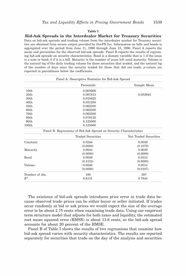
One of the most common proxies for liquidity is the bid-ask spread. Therationale is that dealers require greater compensation for maintaining in-ventories of illiquid assets, and this results in larger bid-ask spreads forilliquid securities. However, as mentioned previously, the bid-ask spreadslisted in the CRSP data are not market data but are merely representativespreads.5 Thus, the magnitude, characteristics, and determinants of bid-askspreads in the Treasury market have not been reliably examined before.Table I provides information on the bid-ask spread for the GovPX data. Al-though we have data for only three days, the bid-ask spread on one day ishighly related to the bid-ask spread on the other two days with a simplecorrelation greater than 0.96. Thus, the bid-ask spread on any one day seemsref lective of general conditions, at least over a short period of time. Theaverage bid-ask spread varies from four-tenths of a cent for the lowest decileto 12.5 cents per $100 for the highest decile, with an average of 5.3 cents.6

3 Balduzzi, Elton, and Green ~1997! examine intraday price changes around economic an-nouncements. They find that a considerable portion of daily price changes can be attributed tothe release of economic news. Moreover, the impact of the economic news usually occurs withinone minute after the announcement and never more than 30 minutes after. Since the lastobserved trade for each bond is almost always after the last announcement in any day, wewould not expect nonsynchronous prices to be an important factor in pricing errors.

4 Using the spline approach described in Section IV, we compare the pricing errors obtainedfrom fitting the CRSP and GovPX data over the period during which GovPX has existed. Usingan identical set of bonds, the correlation of the pricing errors is 0.78. However, fitting theaverage of the bid-ask quotes in CRSP results in slightly smaller pricing errors.

5 See Coleman, Fisher, and Ibbotson ~1992! and our discussion in the preceding section.6 Quote observations are examined if both a bid and ask price are reported. Some of the

reported prices for bonds that did not trade are indicative quotes. Removing these observationshas little effect on the results.


The existence of bid-ask spreads introduces price error in trade data be-cause observed trade prices can be either buyer or seller initiated. If tradesoccur randomly at bid or ask prices we would expect the size of the averageerror to be about 2.75 cents when examining trade data. Using our empiricalterm structure model that adjusts for both taxes and liquidity, the estimatedroot mean squared error ~RMSE! is about 13.6 cents, so the bid-ask spreadaccounts for about 20 percent of the RMSE.

Panel B of Table I shows the results of two regressions that examine howbid-ask spread varies with security characteristics. The results are reportedseparately for securities that trade on the day of the analysis and securities

Table I

Bid-Ask Spreads in the Interdealer Market for Treasury SecuritiesData on bid-ask spreads and trading volume from the interdealer market for Treasury securi-ties are obtained from screen output provided by GovPX Inc. Information on bills and bonds isaggregated over the period from June 11, 1996 through June 13, 1996. Panel A reports themean and percentiles for the observed bid-ask spreads. Panel B reports the results of regress-ing bid-ask spreads on security characteristics. Bond is a dummy variable that is 1 if the issueis a note or bond, 0 if it is a bill. Maturity is the number of years left until maturity. Volume isthe natural log of the daily trading volume for those securities that traded, and the natural logof the number of days since the security traded for those that did not trade. p-values arereported in parentheses below the coefficients.

Panel A: Descriptive Statistics for Bid-Ask Spread

Percentile Sample Mean

10th 0.00390620th 0.007813 0.05294530th 0.01562540th 0.03125050th 0.06250060th 0.06250070th 0.06250080th 0.07812590th 0.125000

100th 0.125000

Panel B: Regressions of Bid-Ask Spread on Security Characteristics

Traded Securities Not Traded Securities

Constant 0.0244 0.0049~0.0000! ~0.1079!

Maturity 0.0044 0.0039~0.0000! ~0.0000!

Bond 0.0029 0.0313~0.4123! ~0.0000!

Volume 20.0046 0.0014~0.0000! ~0.0107!

Number of obs. 190 397R2 0.8131 0.7944


that do not trade that day. Several variables are used to explore how bid-askspreads vary across securities. The variable Bond is a dummy variable thatis 1 if the instrument is a bond and 0 if it is a bill. For bonds and bills thatdo trade, the variable Volume is the natural log of the cumulative tradingvolume. For bonds and bills that do not trade, Volume is the natural log ofthe number of days since it last traded. These variables along with years tomaturity explain about 80 percent of the difference in bid-ask spreads acrosssecurities. The bid-ask spread is negatively related to volume and positivelyrelated to the length of time since the last trade. Furthermore, the bid-askspread increases with maturity and is larger for bonds than for bills.7

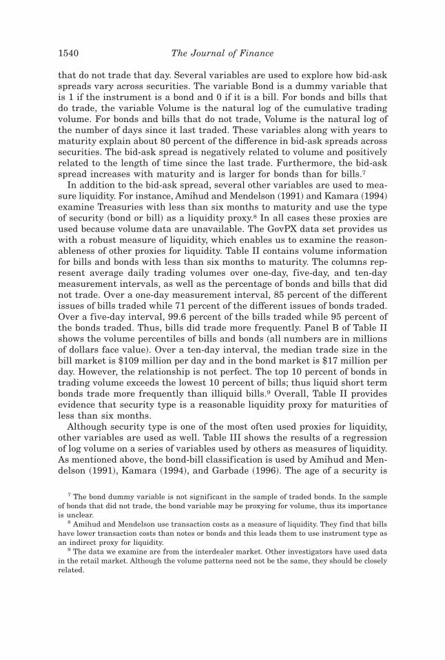
In addition to the bid-ask spread, several other variables are used to mea-sure liquidity. For instance, Amihud and Mendelson ~1991! and Kamara ~1994!examine Treasuries with less than six months to maturity and use the typeof security ~bond or bill! as a liquidity proxy.8 In all cases these proxies areused because volume data are unavailable. The GovPX data set provides uswith a robust measure of liquidity, which enables us to examine the reason-ableness of other proxies for liquidity. Table II contains volume informationfor bills and bonds with less than six months to maturity. The columns rep-resent average daily trading volumes over one-day, five-day, and ten-daymeasurement intervals, as well as the percentage of bonds and bills that didnot trade. Over a one-day measurement interval, 85 percent of the differentissues of bills traded while 71 percent of the different issues of bonds traded.Over a five-day interval, 99.6 percent of the bills traded while 95 percent ofthe bonds traded. Thus, bills did trade more frequently. Panel B of Table IIshows the volume percentiles of bills and bonds ~all numbers are in millionsof dollars face value!. Over a ten-day interval, the median trade size in thebill market is $109 million per day and in the bond market is $17 million perday. However, the relationship is not perfect. The top 10 percent of bonds intrading volume exceeds the lowest 10 percent of bills; thus liquid short termbonds trade more frequently than illiquid bills.9 Overall, Table II providesevidence that security type is a reasonable liquidity proxy for maturities ofless than six months.

Although security type is one of the most often used proxies for liquidity,other variables are used as well. Table III shows the results of a regressionof log volume on a series of variables used by others as measures of liquidity.As mentioned above, the bond-bill classification is used by Amihud and Men-delson ~1991!, Kamara ~1994!, and Garbade ~1996!. The age of a security is

7 The bond dummy variable is not significant in the sample of traded bonds. In the sampleof bonds that did not trade, the bond variable may be proxying for volume, thus its importanceis unclear.

8 Amihud and Mendelson use transaction costs as a measure of liquidity. They find that billshave lower transaction costs than notes or bonds and this leads them to use instrument type asan indirect proxy for liquidity.

9 The data we examine are from the interdealer market. Other investigators have used datain the retail market. Although the volume patterns need not be the same, they should be closelyrelated.


utilized by Sarig and Warga ~1989!, and Warga ~1992! proxies liquidity byindicating whether or not an issue is on-the-run ~the most recently issuedsecurity of a particular maturity!. Additionally, since Ederington and Lee~1993! and Harvey and Huang ~1993! have results which suggest that vol-ume differs over the week, we include dummy variables for each weekday.The set of variables used by others explains a relatively high proportion ofthe variation in volume across securities. About 45 percent of the variationin volume is explained by the independent variables, and all variables ex-cept the Monday dummy variable are significant. However, there is a fairamount of variation in volume that is not explained by the other measuresof liquidity, which suggests that there may be aspects of liquidity not cap-tured by previously used proxies.

Table II

Volume Data for Treasury Bills and Bondswith Less than Six Months to Maturity

Data on trading volume from the interdealer market for Treasury securities are obtained fromGovPX Inc. The reported numbers are for daily volume of all listed noncallable Treasury secu-rities with less than six months to maturity. Panel A reports the percentage of days the secu-rities traded. Panel B reports the percentiles of trading volume. Statistics for the 5- and 10-dayintervals are obtained from overlapping observations of 5 and 10 trading days. The samplecovers June 17, 1991 through September 29, 1995.

Panel A: Trading Percentages

Bills Bonds

MeasurementInterval

TotalObservations

PercentTraded

TotalObservations

PercentTraded

1 Day 30871 85.34 20666 70.805 Days 25766 99.60 19998 94.74

10 Days 23327 99.97 19162 96.91

Panel B: Distribution of Volume ~$ Millions!

Bills Bonds

Percentile 1 Day5-Day

Average10-DayAverage 1 Day

5-DayAverage

10-DayAverage

10th 0 19.6 25.6 0 1.0 2.220th 9 37.8 42.6 0 3.8 5.630th 27 57.4 63.4 1 6.8 8.940th 51 79.6 86.0 2 10.4 12.450th 82 104.4 108.6 6 14.8 16.660th 124 133.2 135.6 11 20.0 21.770th 186 170.6 168.2 20 26.8 27.780th 293 231.8 218.3 34 36.4 35.990th 607 399.0 333.2 63 52.4 49.395th 1124 752.2 565.3 96 69.2 63.8

100th 8215 2756.2 1776.1 4499 925.4 504.8


To provide a better understanding of how liquidity varies across the termstructure, Figure 1 shows the relationship between daily trading volume andmaturity for bonds. There is not a monotonic relationship over the full ma-turity range. Trading volume increases with maturity from six months totwo years. Beyond two years, volume is roughly constant and the same asthat of bonds with two years to maturity. Overall, we find that the liquiditymeasures used by others are related to volume, but none are highly corre-lated with volume across all maturities, and using lesser proxies could in-troduce substantial error.

IV. Pricing Errors in Present Values

Although utilizing the GovPX data provides us with an accurate measureof market clearing prices, errors still exist when cash f lows are discountedusing estimated spot rates. Nonsynchronous trading and the existence ofrandom pricing errors are possible explanations that we will explore againlater in this section. However, there are economic inf luences that could also

Table III

Regression Results of Volume on Liquidity ParametersData from the interdealer market for Treasury securities are obtained from GovPX Inc. Thetable reports the results of an ordinary least squares regression of the natural log of dailytrading volume on the independent variables.

ln~Vol! 5 b0 1 b1 Bill 1 b2 Active 1 b3 Age 1 b4 Monday

1 b5 Tuesday 1 b6 Wednesday 1 b7 Thursday 1 e.

The sample contains information on all noncallable Treasury securities. Bill is 1 if the securityis a bill, and 0 otherwise. Active is 1 if the issue is on-the-run, and 0 otherwise. Age is thenumber of years since issuance. The day-of-the-week dummies are 1 if the observation occurs onthat day, and 0 otherwise. Sample 1 covers October 1, 1991 through February 2, 1992, sample2 covers March 1, 1993 through July 7, 1993, and sample 3 covers May 23, 1995 throughSeptember 29, 1995. The results reported are for the combined sample.

Coefficient t-Statistic p-Value

Constant 3.115 175.158 0.000Bill 0.868 46.315 0.000Active 3.847 128.928 0.000Age 20.182 268.317 0.000Monday 0.023 1.006 0.314Tuesday 0.236 10.994 0.000Wednesday 0.304 14.053 0.000Thursday 0.265 12.159 0.000

R2 0.453Number of obs. 40631


lead to pricing errors, such as liquidity effects, tax effects, and cross-sectional variation in the demand for assets based on their use as collateralin repurchase agreements.

Theory suggests that illiquid bonds will offer higher returns than similar,more liquid bonds. As Amihud and Mendelson ~1991! argue, the bid-ask spreadis part of the cost of trading. In order to compensate marketmakers for mak-ing a market in illiquid assets, and possibly ref lecting a lack of trade infor-mation to discern the market clearing price of infrequently traded bonds,bid-ask spreads are larger for illiquid bonds. Thus, to provide the same re-turn after paying transaction costs, illiquid bonds must offer a higher returnbefore transaction costs. Since our pricing formula does not include trans-action costs, illiquid bonds should trade at prices below the price estimatedusing the present value formula.

Taxes may also affect the relative prices of bonds and lead to errors inestimated prices. One way for this to occur is through the presence of taxclienteles. Investors in different tax brackets may desire bonds with differ-ent characteristics ~see Schaefer ~1982!!. If the marginal investors for twodifferent bonds are taxed at different rates, the relative prices of these bonds

Figure 1. 95th Percentile of the log of daily trading volume grouped by maturity. Thedata points in each maturity range represent the 95th percentile of log volume for all noncall-able bonds that fall into that maturity range. Sample 1 is from October 1, 1991 through Feb-ruary 11, 1992, sample 2 covers March 1, 1993 through July 7, 1993, and sample 3 covers May23, 1995 through September 29, 1995.


will be affected. Another way in which taxes can affect bond prices is throughtax timing options. Tax timing options are associated with the value of beingable to time the sale of a bond to optimize the tax treatment of capital gainsor losses ~see Constantinides and Ingersoll ~1984!!. Moreover, it is importantto note that even if the ordinary income and capital gains tax rates are thesame for all investors, taxes may still enter into the relative prices of bonds.For instance, consider three bonds with different coupons all maturing onthe same day. If all three bonds are discount bonds, or all three are premiumbonds, then the ratio of bonds one and three necessary to match the cashf lows of bond two are the same regardless of whether the cash f lows beingmatched are before or after taxes. However, if bonds one and two are dis-count bonds and bond three is a premium bond, there may be no combina-tion of bonds one and three that will exactly match the after-tax cash f lowsof bond two, due to the constant yield method of amortizing the premium ofbond three. Thus, if the tax rate of the marginal investor is positive, taxesmay have an effect on the relative prices of bonds.

In addition to tax and liquidity effects, there may be shifts in demand orsupply for individual bonds that affect their prices relative to other bonds.Duffie ~1996! argues that securities that are on special in the repo market~i.e., they have overnight borrowing rates that are below the general collat-eral rate! will trade at a premium over similar assets that are not on special.Jordan and Jordan ~1997! examine repo specials and find that they do sig-nificantly impact bond prices. However, their evidence reveals that repo spe-cials alone do not entirely explain the premiums associated with on-the-runissues, suggesting that the high liquidity of these issues has value in itself.Overnight repurchase rates were not reported by GovPX during the timeperiod of our sample, and we are therefore unable to determine which bondswere on special. However, specialness is highly correlated with volume, andmay be a partial explanation for any volume effects we find.

In this paper we use two types of tests for understanding the determi-nants of pricing errors in present values—arbitrage tests and an examina-tion of deviations from a term structure fit. We examine each in turn.

A. Arbitrage Tests

Tests that are based on the principle of no arbitrage are extremely pow-erful because they do not rely on a valuation model and require only mini-mal assumptions about preferences. Arbitrage style tests have a long historyin examining the determinants of government bond prices ~see Litzenbergerand Rolfo ~1984b!, Jordan and Jordan ~1991!, and Ronn and Shin ~1997!!.However, these authors examine quite small samples ~30 to 40 observa-tions!, and thus are constrained to look exclusively at tax effects. Our dailydata and access to trading volume allow us to use triplets to examine bothtax timing and liquidity effects.

The arbitrage test commonly used to examine tax timing, tax clientele,and tax regime effects involves the use of bond triplets, three bonds with thesame maturity but different coupons. Assuming a zero tax rate for the mo-


ment, for each triplet let Ci and Pi be the coupon and price of bond i, wherei 5 1,2,3 and the bonds are arranged in ascending order by coupon. The lawof one price states that

P2 5 xP1 1 ~1 2 x!P3, ~1!

where

x 5C2 2 C3

C1 2 C3.

Equation ~1! must hold because in the proportions shown the cash f lows arethe same for bond two and the portfolio of bonds one and three. When taxesare present, equation ~1! needs to be modified. First, if bondholders are taxedwhen capital gains and losses are realized, then a tax timing option may bepresent. If the portfolio always moves exactly as bond two, they would beequally desirable. However, as long as there are states of the world wherethey move differently, the portfolio of bonds one and three is more valuablethan bond two, and a tax timing option exists. This is an application of theprinciple that a portfolio of options is more valuable than an option on the port-folio. When a tax timing option is present, equation ~1! will be an inequality.

To examine the effects of tax timing options, it is necessary to eliminateother tax inf luences by ensuring that the pretax and posttax cash f lows arethe same. Since premium and discount bonds are treated differently for taxpurposes, the effect of tax timing options is unequivocal only if all threebonds are premium or discount bonds. Because of the lack of a significantnumber of discount triplet observations, we focus on premium triplets. Theamortization of bond premiums also needs to be considered. The Tax ReformAct of 1986 altered the amortization of bonds. Bonds issued before Septem-ber 28, 1985 ~old bonds! may be amortized using the straight-line method,which makes them preferable to bonds issued after that date ~new bonds!which must use the constant yield method. Thus, initially we examine onlytriplets where all three bonds were issued before or after September 28,1985. Finally, because the tax timing involves controlling the year of thegain or loss, we do not include bonds with less than one year to maturity.

The measure we use to quantify the tax timing and liquidity effects in bondtriplet prices is the difference between the price of bond two and the replicat-ing portfolio of bonds one and three. In equation form this difference is:

D 5 P2 2 ~xP1 1 ~1 2 x!P3!. ~2!

If there is a tax timing option, bond two should be less expensive than theportfolio of bonds one and three and D should be less than zero. Table IVreports our results.10 For triplets consisting of new bonds ~the first row of

10 The hypothesis tested is that the percentage of triplet observations with D less than 0 isequal to 102 using the property that 2~sin21!p 2 sin21%0.5!0!n is distributed standard normalin the limit, where p is the proportion of observations where D is greater than 0 and n is thenumber of observations ~Litzenberger and Rolfo ~1984b!!.


Table IV

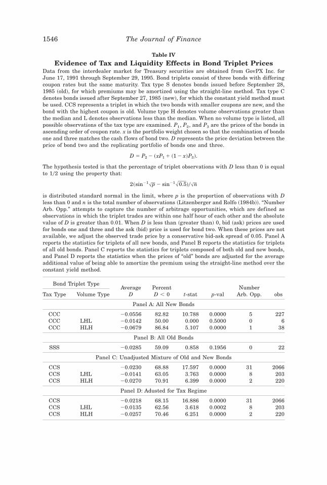
Evidence of Tax and Liquidity Effects in Bond Triplet PricesData from the interdealer market for Treasury securities are obtained from GovPX Inc. forJune 17, 1991 through September 29, 1995. Bond triplets consist of three bonds with differingcoupon rates but the same maturity. Tax type S denotes bonds issued before September 28,1985 ~old!, for which premiums may be amortized using the straight-line method. Tax type Cdenotes bonds issued after September 27, 1985 ~new!, for which the constant yield method mustbe used. CCS represents a triplet in which the two bonds with smaller coupons are new, and thebond with the highest coupon is old. Volume type H denotes volume observations greater thanthe median and L denotes observations less than the median. When no volume type is listed, allpossible observations of the tax type are examined. P1, P2, and P3 are the prices of the bonds inascending order of coupon rate. x is the portfolio weight chosen so that the combination of bondsone and three matches the cash f lows of bond two. D represents the price deviation between theprice of bond two and the replicating portfolio of bonds one and three.

D 5 P2 2 ~xP1 1 ~1 2 x!P3!.

The hypothesis tested is that the percentage of triplet observations with D less than 0 is equalto 102 using the property that:

2~sin21!p 2 sin21%0.5!0!n

is distributed standard normal in the limit, where p is the proportion of observations with Dless than 0 and n is the total number of observations ~Litzenberger and Rolfo ~1984b!!. “NumberArb. Opp.” attempts to capture the number of arbitrage opportunities, which are defined asobservations in which the triplet trades are within one half hour of each other and the absolutevalue of D is greater than 0.01. When D is less than ~greater than! 0, bid ~ask! prices are usedfor bonds one and three and the ask ~bid! price is used for bond two. When these prices are notavailable, we adjust the observed trade price by a conservative bid-ask spread of 0.05. Panel Areports the statistics for triplets of all new bonds, and Panel B reports the statistics for tripletsof all old bonds. Panel C reports the statistics for triplets composed of both old and new bonds,and Panel D reports the statistics when the prices of “old” bonds are adjusted for the averageadditional value of being able to amortize the premium using the straight-line method over theconstant yield method.

Bond Triplet Type

Tax Type Volume TypeAverage

DPercentD , 0 t-stat p-val

NumberArb. Opp. obs

Panel A: All New Bonds

CCC 20.0556 82.82 10.788 0.0000 5 227CCC LHL 20.0142 50.00 0.000 0.5000 0 6CCC HLH 20.0679 86.84 5.107 0.0000 1 38

Panel B: All Old Bonds

SSS 20.0285 59.09 0.858 0.1956 0 22

Panel C: Unadjusted Mixture of Old and New Bonds

CCS 20.0230 68.88 17.597 0.0000 31 2066CCS LHL 20.0141 63.05 3.763 0.0000 8 203CCS HLH 20.0270 70.91 6.399 0.0000 2 220

Panel D: Adusted for Tax Regime

CCS 20.0218 68.15 16.886 0.0000 31 2066CCS LHL 20.0135 62.56 3.618 0.0002 8 203CCS HLH 20.0257 70.46 6.251 0.0000 2 220


Panel A!, the portfolio is more expensive than bond two in 83 percent of the227 observations, with an average price difference of six cents per $100 facevalue. For triplets that include only old bonds, in 60 percent of the 22 ob-servations the portfolio is more costly, with an average difference of threecents. These results are similar to those reported by others. Our access tosuperior data and a much larger number of observations ~others have 30 to40 observations! does not refute the sign or magnitude of pricing differencesbetween bond triplets.

However, our much larger sample does allow us to explore whether theseresults could be due to liquidity rather than tax timing effects. In order tolook for evidence of liquidity effects, bonds are separated into high and lowvolume groups based on whether the daily volume for each bond is above orbelow the median volume for all bonds on that day. Less liquid bonds shouldhave lower prices and offer higher returns. A considerable difference in li-quidity between bond two and the bonds in the portfolio should alter therelationship between their prices. When bond two is less liquid than theportfolio ~designated by HLH in Table IV!, then ceteris paribus we wouldexpect bond two to be cheaper and D to be more negative. On the other hand,when bond two is more liquid than the portfolio ~designated by LHL inTable IV!, we would expect D to be less negative or positive if liquidity ef-fects dominate the tax timing effects. Panel A of Table IV shows the results.In both cases, sorting by liquidity affects the relationship in the direction wewould theorize. However, D is always negative, indicating that both tax tim-ing and liquidity effects are present. The difference caused by liquidity isapproximately 5 cents per $100 face value.11

By recognizing the different tax treatment of bonds issued before and af-ter September 29, 1985 ~old and new bonds!, we can dramatically expandour sample size, which is important for distinguishing between the effects ofliquidity and taxes. The type of triplet for which we have a substantial num-ber of observations contains two new bonds and one old, with bond threebeing the old bond. Since old bonds have a tax advantage, examining tripletsin which the highest coupon bond is old should result in an increase in theprice of bond three and a more negative D. Panel C in Table IV analyzes thiscase. We have 2,066 observations. The average difference in price betweenbond two and the replicating portfolio is approximately three cents, with theportfolio being more expensive 69 percent of the time.

Although the average D is negative, it is actually closer to zero than in theall old or all new triplets. This is inconsistent with the tax advantage of oldbonds being priced. Using a t-test, we find that the average D for triplets

11 At the suggestion of the referee, we also pool the triplet observations together and regressD on dummy variables for the three cases we consider and a liquidity parameter that is theweighted average of volumes for bonds one and three over the volume for bond two. We findthat CCC and CCS are significantly less than zero, and the magnitudes of the coefficients aresimilar to the average D’s listed in the table. The liquidity term is not found to be significantlydifferent from zero.


consisting of two new bonds and one old bond is significantly ~at the 0.01level! greater than the average D for triplets consisting of all new bonds. Inother words, we find no evidence that the difference in tax treatment of oldand new bonds is ref lected in market prices, which is in contrast to thefindings of Ronn and Shin ~1997!. One explanation for this difference is thatthey examine triplet data from 1985 through 1990, whereas our data arefrom 1991 through 1995. Moreover, given their time frame, they comparetriplets of all old bonds to triplets containing one or more new bonds, whereaswe compare triplets of all new bonds to triplets containing one old bond. Thelower part of Panel C splits the sample by liquidity to see if the results couldbe due to liquidity differences. Once again, changes in D are consistent withliquidity and tax timing effects. When bond two is more liquid than theportfolio, D is less negative, as we would expect. Likewise, when bond two isless liquid than the portfolio, D increases but is still negative. Evidence froma t-test indicates that the average D for the HLH group is significantly lessthan the average D for the LHL group at the 0.01 level.

By adjusting the price of the old bonds by the expected discounted value ofits preferential tax treatment, we can compare this adjusted price with theprices of the other two bonds on a common tax basis.12 The results are shownin Panel D of Table IV. As we would expect, D becomes less negative afterdecreasing the price of bond three by the value of the tax advantage. Noneof the previous results change.

The second to last column provides information on the number of potentialarbitrage opportunities. The existence of arbitrage opportunities is interest-ing because it provides evidence that either tax clienteles have an impact onthe prices of bonds, or markets are not efficient. Table IV reports the num-ber of observations in which the last trade prices of the three bonds arerecorded within a half hour of each other and the difference in price betweenbond two and the portfolio is greater than 1 cent when using the appropriatebid or ask prices. Specifically, when D is less than ~greater than! zero, theask ~bid! prices are examined for bonds one and three and the bid ~ask! priceis used for bond two. When necessary the observed trade prices are adjustedby a conservative bid-ask spread of 5 cents to estimate the other quote. Theonly way for there to be a substantial number of mispricings between bondtwo and the portfolio is for there to exist tax clienteles who place differentvalues on the bond triplets. The number of violations are sufficiently fewthat there is little support for the existence of tax clienteles or inefficiency.In summary, the bond triplets provide evidence of a liquidity effect and taxtiming options. However, examining bond triplets does not provide evidencethat the difference in tax treatment of old and new bonds is ref lected inmarket prices or that tax clienteles affect prices.

12 The adjustment is made by calculating the amortization schedule for old and new bondsfor all maturities and premiums, and discounting these differences by the estimated spot rates.This difference is the added value we would expect to see given the preferential treatment of oldbonds, which may or may not be ref lected in observed bond prices.


Arbitrage tests depend on having two portfolios with identical cash f lows.Bond triplets are one way to construct these portfolios. However, there aremany other possibilities. To further explore the effect of liquidity, we use anew approach in which we construct portfolios with more than three bonds.This allows us to create portfolios with more extreme differences in liquidity.Each day two portfolios are created with an equal number of bonds of con-secutive maturities. In each portfolio there is a bond that matures every sixmonths, which enables us to match cash f lows at each maturity. One port-folio is constructed from one of each high volume bond, the other portfoliocontains low volume bonds held in ~strictly positive! proportions such thatthey match the cash f lows of the high volume portfolio. The law of one priceimplies they should have the same price if liquidity is unimportant. If li-quidity does have value, then the low volume portfolio should have a lowerprice. Tax timing should not be an important consideration because the port-folios have roughly the same number of bonds.

In order to obtain a large number of observations, we examine bonds thathave cash f lows in February and August. Whenever possible, we choose bondswith February 15 and August 15 as the cash f low dates. If more than twobonds of a given maturity trade on the same day, the two that have thegreatest difference in volume are selected. In cases where two bonds do notexist with these coupons dates, we include bonds that mature at the end ofthe month. In sample 1 there are 30 out of 762 bonds that do not pay on the15th of the month, in sample 2 there are 56 of 608, and in sample 3 there are189 of 626.13 When the cash f low dates differ, we adjust the cash f lows bythe forward rate. If one of the portfolio bonds does not pay on the 15th, itscash f lows are adjusted to the 15th using the forward rate for that portfolio.The magnitude of this correction is very small compared to the difference inprices of the two portfolios. Furthermore, the frequency of adjustment isroughly the same for the high and low volume group; thus errors in adjust-ing cash f lows should not affect the results. We include as many periods aspossible given that cash f lows have to match and no payments can differ bymore than 16 days. We require there to be at least five bonds in each port-folio. The maturity of the portfolios varies between 2½ and 5 years, with themedian number of years being between 3 and 3½ years.

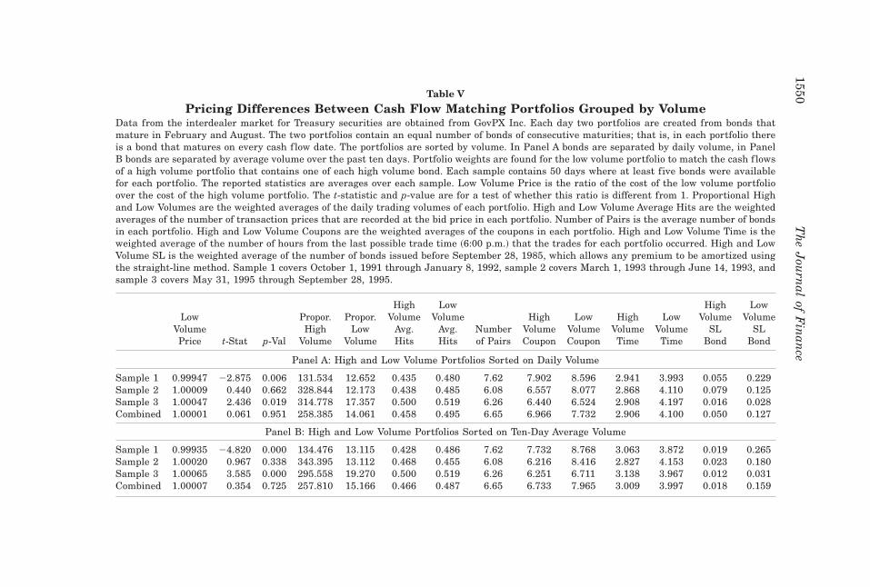
Table V shows the volume for the high volume portfolio and the low vol-ume portfolio where volume is measured over one day in Panel A and overten days in Panel B. The average volume difference between the two groupsis substantial. To get an idea of the magnitude of this difference, we canconsult Table II. Although Table II is restricted to bonds with less than sixmonths to maturity, the high volume shown in Table V would lie in the topdecile and the low volume in the lower four deciles. Although there doesappear to be a significant volume difference between portfolios, Table V does

13 Each sample contains 50 days in which at least five bonds are available for each portfolio.Sample 1 is taken from October 2, 1991 through January 8, 1992, sample 2 covers March 3,1993 through June 14, 1993, and sample 3 covers May 31, 1995 through September 28, 1995.


Table V

Pricing Differences Between Cash Flow Matching Portfolios Grouped by VolumeData from the interdealer market for Treasury securities are obtained from GovPX Inc. Each day two portfolios are created from bonds thatmature in February and August. The two portfolios contain an equal number of bonds of consecutive maturities; that is, in each portfolio thereis a bond that matures on every cash f low date. The portfolios are sorted by volume. In Panel A bonds are separated by daily volume, in PanelB bonds are separated by average volume over the past ten days. Portfolio weights are found for the low volume portfolio to match the cash f lowsof a high volume portfolio that contains one of each high volume bond. Each sample contains 50 days where at least five bonds were availablefor each portfolio. The reported statistics are averages over each sample. Low Volume Price is the ratio of the cost of the low volume portfolioover the cost of the high volume portfolio. The t-statistic and p-value are for a test of whether this ratio is different from 1. Proportional Highand Low Volumes are the weighted averages of the daily trading volumes of each portfolio. High and Low Volume Average Hits are the weightedaverages of the number of transaction prices that are recorded at the bid price in each portfolio. Number of Pairs is the average number of bondsin each portfolio. High and Low Volume Coupons are the weighted averages of the coupons in each portfolio. High and Low Volume Time is theweighted average of the number of hours from the last possible trade time ~6:00 p.m.! that the trades for each portfolio occurred. High and LowVolume SL is the weighted average of the number of bonds issued before September 28, 1985, which allows any premium to be amortized usingthe straight-line method. Sample 1 covers October 1, 1991 through January 8, 1992, sample 2 covers March 1, 1993 through June 14, 1993, andsample 3 covers May 31, 1995 through September 28, 1995.

LowVolumePrice t-Stat p-Val

Propor.High

Volume

Propor.Low

Volume

HighVolume

Avg.Hits

LowVolume

Avg.Hits

Numberof Pairs

HighVolumeCoupon

LowVolumeCoupon

HighVolume

Time

LowVolume

Time

HighVolume

SLBond

LowVolume

SLBond

Panel A: High and Low Volume Portfolios Sorted on Daily Volume

Sample 1 0.99947 22.875 0.006 131.534 12.652 0.435 0.480 7.62 7.902 8.596 2.941 3.993 0.055 0.229Sample 2 1.00009 0.440 0.662 328.844 12.173 0.438 0.485 6.08 6.557 8.077 2.868 4.110 0.079 0.125Sample 3 1.00047 2.436 0.019 314.778 17.357 0.500 0.519 6.26 6.440 6.524 2.908 4.197 0.016 0.028Combined 1.00001 0.061 0.951 258.385 14.061 0.458 0.495 6.65 6.966 7.732 2.906 4.100 0.050 0.127

Panel B: High and Low Volume Portfolios Sorted on Ten-Day Average Volume

Sample 1 0.99935 24.820 0.000 134.476 13.115 0.428 0.486 7.62 7.732 8.768 3.063 3.872 0.019 0.265Sample 2 1.00020 0.967 0.338 343.395 13.112 0.468 0.455 6.08 6.216 8.416 2.827 4.153 0.023 0.180Sample 3 1.00065 3.585 0.000 295.558 19.270 0.500 0.519 6.26 6.251 6.711 3.138 3.967 0.012 0.031Combined 1.00007 0.354 0.725 257.810 15.166 0.466 0.487 6.65 6.733 7.965 3.009 3.997 0.018 0.159

1550T

he

Jou

rnal

ofF

inan

ce

not support a liquidity effect. The portfolios are normalized so that the highvolume portfolio costs $1. The average cost of the low volume portfolio is shownin column 1. It is significantly different from one in sample 1 and sample 3,but in opposite directions, and overall it is insignificantly different from one.

To compare the value of one portfolio relative to the other, we match pretaxcash f lows. To test whether tax effects may drive our results, we use coupon asa proxy for tax effects and regress the ratio of prices on the difference betweenthe weighted average coupons for the high and low volume portfolios. Differ-ence in coupon is insignificant in explaining the difference in price betweenthe portfolios for both those sorted by 1-day volume and by 10-day volume.

The results may also be inf luenced by nonsynchronous trading. Table Vprovides information on the weighted average of the number of hours before6:00 p.m. EST that the last trade occurred. As expected, the low volumetrades are older on average by about one hour. Potentially, prices could befalling over the day on average and the low volume prices could be an over-estimate of the synchronous price. To test for this, on each day we adjustedthe earlier price to the later price by using the average return over the dayfor all bonds adjusted to the appropriate time interval. The prices move upsome days and down other days in our sample, and the adjustment results inessentially identical results.

Finally, since we use trade data it is possible that we do not find a sig-nificant liquidity effect because our high volume observations are associatedwith bid prices, and our low volume observations are associated with askprices. Columns 6 and 7 show the proportion of the trades that are at the bidprice. Compared to the high volume portfolio, there is some tendency for theobserved trade prices for bonds in the low volume portfolio to occur moreoften at the bid price. We would expect this to make the low volume portfolioless expensive than the high volume portfolio. However, we find little evi-dence that the low volume portfolio is less expensive than the high volumeportfolio, and there seems to be no relation between the difference in port-folio prices and the difference in proportions of bid trades. Thus, bid-askspread is not an explanation for the price differences in portfolios.

Overall, the general arbitrage results provide mixed support for liquidityand tax effects in bond prices. We find evidence that tax-timing options havea significant, if economically small, impact on the prices of Treasury securities.However, we do not find evidence that the differential tax treatment of bondsissued before September 28, 1985 is ref lected in bond prices. When examiningbond triplets, we find that the effects of liquidity are significant but small. Onthe other hand, we find no strong support for either tax or liquidity effects whenwe examine cash f low matching portfolios of consecutive maturities.

B. Term Structure Tests

In order to study the effects of taxes and liquidity over the entire spectrumof maturities, it is necessary to first specify a model of the term structure.Once a model is selected, we can fit it to the after-tax cash f lows of bonds


and thus infer the tax rate faced by the marginal investor. If the estimatedtax rate is significantly different from zero, we can conclude that taxes doaffect the prices of bonds. The after-tax term structure is first estimated byMcCulloch ~1975! assuming a given set of tax rates. Litzenberger and Rolfo~1984a! use a grid search to determine the optimal tax rates implied by thedata. More recently, Green and Ødegaard ~1997! look for a structural changein the implied taxes before and after the change in tax law in 1986. Theyfind that the tax rate of the marginal investor is positive before 1986, butclose to zero afterwards. We use a similar procedure and include an addi-tional parameter to capture the effects of liquidity.

When selecting a model of the term structure, a choice has to be madebetween two different approaches. One approach estimates the term struc-ture each period using only the information contained in the cross section ofbond prices; the other approach constrains the term structure to move witha limited set of state variables, but allows the model to be estimated onceover the entire sample. In general, the benefit of cross-sectional models isthat they provide a better fit than structural models. The cost is that themodel has to be estimated each period, and it is not possible to estimate asingle tax rate for the entire sample period. Since we are interested in pric-ing bonds as accurately as possible, and since there exists no structuralmodel that clearly dominates the f lexible form method, we use nonlinearleast squares to fit Litzenberger and Rolfo’s ~1984a! cubic spline to the after-tax cash f lows of bonds in each period.14

In order to capture the effects of liquidity on the relative prices of bonds,we add a liquidity term ~log volume! to the reduced form price equation.There are four pricing scenarios for tax purposes: discount bonds issuedbefore and after July 18, 1984, and premium bonds issued before and afterSeptember 28, 1985.15 Under each tax scenario, we solve for price as a non-linear function of the tax rate and the parameters of the discount function.To these price functions we add log volume to capture the effects of liquidityon prices. This specification of how liquidity affects prices is ad hoc, but isdone with tractability in mind. The reduced form price function under thevarious tax regulations is a nonlinear function of the tax rate and the pa-rameters of the discount function and can be quite complicated. We want to

14 There is an abundant literature on splines. See Shea ~1984! for a discussion of the issues.Using simulated data, Beim ~1992! finds that cubic splines perform as well as or better thanother estimation techniques. The methodology we use is along the lines of Litzenberger andRolfo ~1984a!. Breakpoints for the spline functions are chosen at 1, 2, and 4 years to maturity.Although it is common to use more breakpoints, we use relatively few to guard against over-fitting the data. We use nonlinear regressions to allow for the nonlinear interaction betweenthe tax rate and the parameters of the discount function ~see Langetieg and Smoot ~1989! forevidence of the advantage of nonlinear methods over the instrumental variable approach usedin Litzenberger and Rolfo ~1984a!!. In order to examine whether the results are sensitive to theparticular f lexible form chosen, we also fit the data using the Nelson and Siegel methodologyand find similar results in terms of magnitude and significance.

15 See Green and Ødegaard ~1997!, Ronn and Shin ~1997!, or Fabozzi and Nirenberg ~1991!for the precise treatment of discount and premium bonds under the different tax regulations.


allow for the presence of liquidity effects without complicating this functionfurther. We examine maturities less than or equal to 10 years. Trade datafor long term bonds are relatively sparse, with an average of about fiveobservations a day for maturities greater than 10 years. It has been shownthat fitting the curve at long maturities with few observations can lead tospurious results ~see Shea ~1984!!.

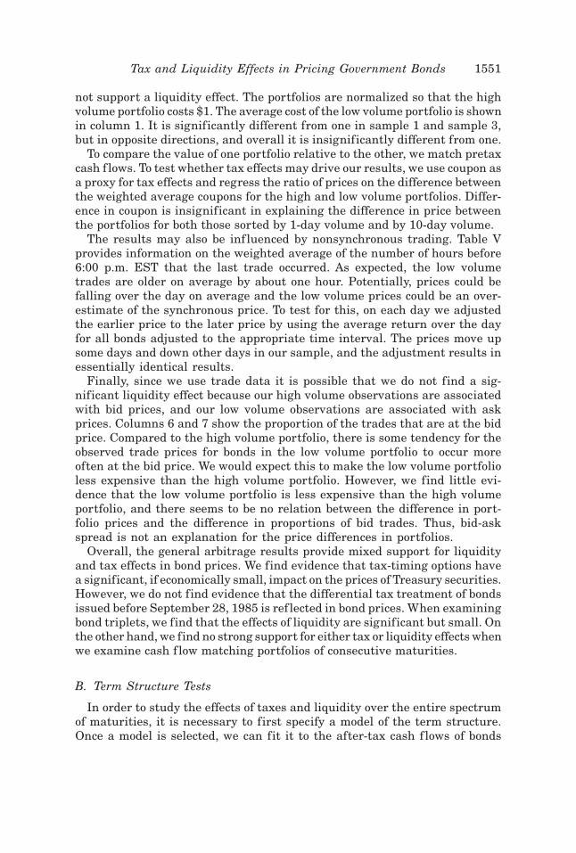
Table VI reports the root mean squared errors and the average estimatedtax rate and liquidity parameter for three subsamples of 90 days of data aswell as for the combined sample.16 Including tax and liquidity terms im-proves the fit across all maturities except for those less than one year. Theaverage estimated tax rate over the three subsamples is 8 percent. We findthat the tax rate is statistically significant 69 times in the first sample, but

16 Sample 1 covers October 1, 1991 through February 11, 1992, sample 2 covers March 1,1993 through July 7, 1993, and sample 3 covers May 23, 1995 through September 29, 1995.

Table VI

Estimated Tax and Liquidity ParametersData from the interdealer market for Treasury securities are obtained from GovPX Inc. Theafter-tax term structure is fitted with a cubic spline. Log of volume is added to the reduced formprice equation for all bonds to capture the effects of liquidity. The tax and liquidity terms areestimated simultaneously with the spline parameters in a nonlinear regression. Panel A reportsthe root mean squared errors ~pooled over the combined sample! when the tax rate and liquidityterms are estimated freely or constrained to be zero. Panel B reports the mean estimated taxand liquidity parameters for the three samples. Also reported are the number of instanceswhere the parameters are significant at the 0.05 level, using heteroskedasticity-consistent stan-dard errors ~Mackinnon and White ~1985!!. Sample 1 covers October 1, 1991 through February8, 1992, sample 2 covers March 1, 1993 through July 7, 1993, and sample 3 covers May 23, 1995through September 29, 1995.

Panel A: Root Mean Squared Errors

MaturityTax 5 0

Liquidity 5 0 Tax 5 0 Liquidity 5 0Both Est.

Freely

,1 0.0528 0.0902 0.0694 0.09831–3 0.1483 0.1356 0.1471 0.13203–5 0.1623 0.1422 0.1476 0.12945–10 0.2373 0.2088 0.2132 0.1892

All maturities 0.1566 0.1441 0.1480 0.1363

Panel B: Parameter Means

Tax RateNumber

Sig.0Sample LiquidityNumber

Sig.0Sample

Sample 1 0.1270 69090 0.0328 62090Sample 2 0.0318 11090 0.0225 55090Sample 3 0.0851 18090 0.0121 43090Combined 0.0813 980270 0.0225 1600270


only 11 and 18 times in the second and third samples.17 This is evident inthe pattern of estimated tax rates, as shown in Figure 2. Although the es-timated tax rates do exhibit considerable volatility, it is evident that theestimated tax rates are small, especially in samples 2 and 3. This confirmsthe findings of Green and Ødegaard ~1997!, who find the estimated tax rateduring the 1987–1992 period to be close to zero.

Although we find little evidence of tax effects, it is worth noting that theassumptions commonly made to estimate the after-tax term structure implythat differences between capital gains and ordinary income tax rates havelittle impact on prices. For instance, it is common to assume that all bondsare held to maturity. Thus, the only capital gains are for bonds selling at adiscount, and the only losses come from premium bonds. Moreover, the cap-ital gains tax rate only enters the valuation process for bonds issued beforeJuly 18, 1984 and selling at a discount. If they are issued after this date, alldiscounts are taxed at the ordinary rate. In all three of our subsamples, weobserve no bonds issued before July 18, 1984 that traded at a discount. Thus,we have little hope of distinguishing between the tax rate on capital gainsand ordinary income. Since the trade-off between these two rates is a majorcontributor to any tax effects, it is not surprising that we do not find con-vincing evidence of their existence. In the case of bond triplets, no assump-tion on the holding period is necessary, and we do find some evidence oftax-timing options, although the magnitude of the effects is quite small.

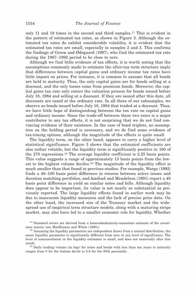
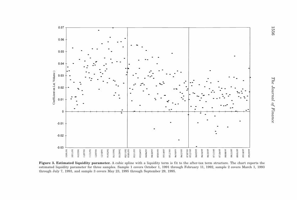
The liquidity term, on the other hand, appears to carry a higher level ofstatistical significance. Figure 3 shows that the estimated coefficients arealso rather volatile, but the liquidity term is significantly positive in 160 ofthe 270 regressions.18 The average liquidity coefficient is 2.25 basis points.This value suggests a range of approximately 13 basis points from the low-est to the highest volume deciles.19 The magnitude of the liquidity effect ismuch smaller than that found in previous studies. For example, Warga ~1992!finds a 40–100 basis point difference in returns between active issues andduration matching portfolios, and Amihud and Mendelson ~1991! report a 40basis point difference in yield on similar notes and bills. Although liquiditydoes appear to be important, its value is not nearly as substantial as pre-viously reported. The large liquidity effects found in earlier work may bedue to inaccurate liquidity measures and the lack of precise price data. Onthe other hand, the increased size of the Treasury market and the wide-spread use of empirical term structure models, along with a maturing stripsmarket, may also have led to a smaller economic role for liquidity. Whether

17 Standard errors are derived from a heteroskedasticity-consistent estimate of the covari-ance matrix ~see MacKinnon and White ~1985!!.

18 Assuming the liquidity parameters are independent draws from a normal distribution, themean liquidity parameter is significantly different from zero at any level of significance. Thelevel of autocorrelation in the liquidity estimates is small, and does not materially alter thisresult.

19 Daily trading volume ~in logs! for notes and bonds with less than ten years to maturityranges from 0 for the bottom decile to 5.8 for the 95th percentile.


Figure 2. Estimated tax rates. A cubic spline with a liquidity term is fit to the after-tax term structure. The chart reports the estimated taxrates for three samples. Sample 1 covers October 10, 1991 through February 11, 1992, sample 2 covers March 1, 1993 through July 7, 1993, andsample 3 covers May 23, 1995 through September 29, 1995.

Tax

and

Liqu

idity

Effects

inP

ricing

Govern

men

tB

ond

s1555

Figure 3. Estimated liquidity parameter. A cubic spline with a liquidity term is fit to the after-tax term structure. The chart reports theestimated liquidity parameter for three samples. Sample 1 covers October 1, 1991 through February 11, 1992, sample 2 covers March 1, 1993through July 7, 1993, and sample 3 covers May 23, 1995 through September 29, 1995.

1556T

he

Jou

rnal

ofF

inan

ce

the diminished role of liquidity we observe is due to the use of more precisedata or is a result of the increased efficiency of the Treasury market isunclear. In either case, our overall finding is that the current economic roleof liquidity in the relative prices of Treasury securities is quite small.

The inconsequential tax and liquidity effects that we find suggest thatmore bonds can be included in term structure estimation. Market partici-pants commonly narrow the pool of bonds they consider when estimating theterm structure in order to use bonds they believe are unaffected by tax andliquidity effects. Our evidence implies that a larger sample of bonds can beused to estimate the term structure, which could lead to smaller estimationerror. The small liquidity effects we observe also have relevance for the trade-off between the larger bid-ask spreads and higher expected returns of illiq-uid bonds, which is relevant to investors who must decide whether to holdilliquid bonds.

Table VI and Figure 1 may provide some explanation as to why we do notfind convincing evidence of liquidity effects in the arbitrage tests, yet we doobserve liquidity effects in the term structure estimation. The arbitrage testsutilize bonds near the short end of the maturity spectrum in order to comeup with enough issues to match cash f lows. Neither the bond triplet ap-proach nor the cash f low matching approach utilize bonds with more thanfive years to maturity. However, Figure 1 shows that many of the highlyliquid bonds have maturities greater than five years. Moreover, Table VIshows that the reduction in pricing errors by including the liquidity term isstrongest for longer maturity bonds. Thus, the term structure approach ismore robust in that it allows us to examine liquidity over a broader range ofmaturities.

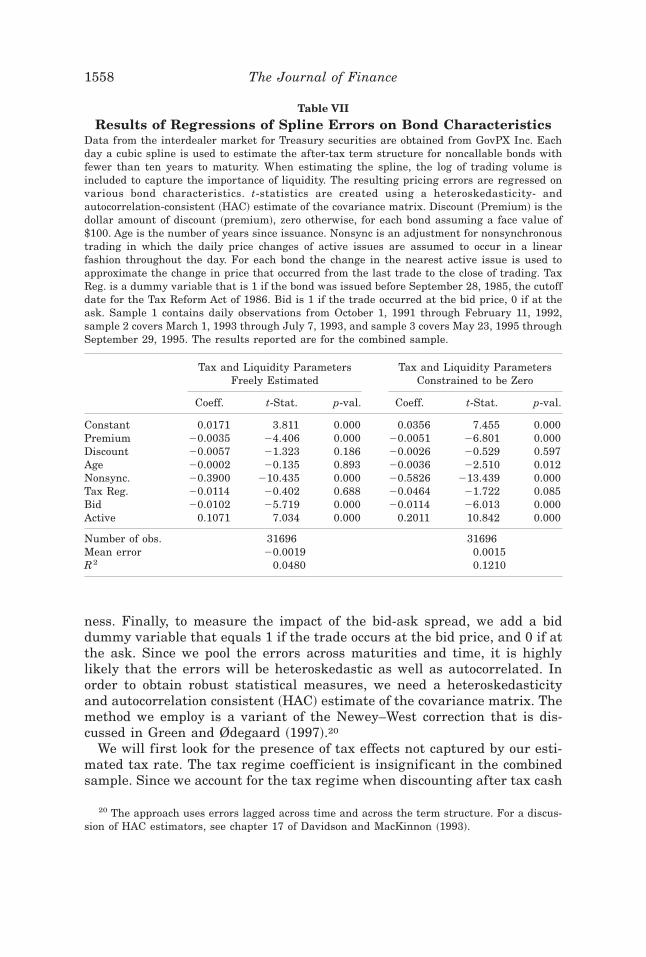
The average root mean squared error is 0.1363 per $100 face value, orabout 14 basis points. As discussed previously, the average bid-ask spreadfor notes and bonds is 0.053. Thus, roughly 20 percent of the root meansquared error can be attributed to the bid-ask spread since we fit the curveto trade data. To examine whether remaining errors are systematically re-lated to certain bond attributes, we regress pricing errors on a series of bondcharacteristics. The results are reported in Table VII. The left column re-ports the regression results when the tax and liquidity parameter are esti-mated freely. The right column reports the results when the two terms areconstrained to be zero. In order to capture the effects of tax timing options,which are not explicitly modeled in the after-tax cash f lows, we include thedollar premium or discount. We also use an age variable to examine whetherthere are remaining liquidity effects not captured by our liquidity term. Wealso include a measure of nonsynchroneity. The nonsynchronous variable isthe daily price change in the nearest active issue times the fraction of theday between the last trade and 6:00 p.m. EST. A tax regime dummy variableis utilized that equals 1 if the bond trades at a premium and is issued beforeSeptember 28, 1985; this is meant to capture the preferential amortizationrules for old bonds. Another dummy variable set equal to 1 is used if theissue is on-the-run; this is designed to capture the effects of repo special-


ness. Finally, to measure the impact of the bid-ask spread, we add a biddummy variable that equals 1 if the trade occurs at the bid price, and 0 if atthe ask. Since we pool the errors across maturities and time, it is highlylikely that the errors will be heteroskedastic as well as autocorrelated. Inorder to obtain robust statistical measures, we need a heteroskedasticityand autocorrelation consistent ~HAC! estimate of the covariance matrix. Themethod we employ is a variant of the Newey–West correction that is dis-cussed in Green and Ødegaard ~1997!.20

We will first look for the presence of tax effects not captured by our esti-mated tax rate. The tax regime coefficient is insignificant in the combinedsample. Since we account for the tax regime when discounting after tax cash

20 The approach uses errors lagged across time and across the term structure. For a discus-sion of HAC estimators, see chapter 17 of Davidson and MacKinnon ~1993!.

Table VII

Results of Regressions of Spline Errors on Bond CharacteristicsData from the interdealer market for Treasury securities are obtained from GovPX Inc. Eachday a cubic spline is used to estimate the after-tax term structure for noncallable bonds withfewer than ten years to maturity. When estimating the spline, the log of trading volume isincluded to capture the importance of liquidity. The resulting pricing errors are regressed onvarious bond characteristics. t-statistics are created using a heteroskedasticity- andautocorrelation-consistent ~HAC! estimate of the covariance matrix. Discount ~Premium! is thedollar amount of discount ~premium!, zero otherwise, for each bond assuming a face value of$100. Age is the number of years since issuance. Nonsync is an adjustment for nonsynchronoustrading in which the daily price changes of active issues are assumed to occur in a linearfashion throughout the day. For each bond the change in the nearest active issue is used toapproximate the change in price that occurred from the last trade to the close of trading. TaxReg. is a dummy variable that is 1 if the bond was issued before September 28, 1985, the cutoffdate for the Tax Reform Act of 1986. Bid is 1 if the trade occurred at the bid price, 0 if at theask. Sample 1 contains daily observations from October 1, 1991 through February 11, 1992,sample 2 covers March 1, 1993 through July 7, 1993, and sample 3 covers May 23, 1995 throughSeptember 29, 1995. The results reported are for the combined sample.

Tax and Liquidity ParametersFreely Estimated

Tax and Liquidity ParametersConstrained to be Zero

Coeff. t-Stat. p-val. Coeff. t-Stat. p-val.

Constant 0.0171 3.811 0.000 0.0356 7.455 0.000Premium 20.0035 24.406 0.000 20.0051 26.801 0.000Discount 20.0057 21.323 0.186 20.0026 20.529 0.597Age 20.0002 20.135 0.893 20.0036 22.510 0.012Nonsync. 20.3900 210.435 0.000 20.5826 213.439 0.000Tax Reg. 20.0114 20.402 0.688 20.0464 21.722 0.085Bid 20.0102 25.719 0.000 20.0114 26.013 0.000Active 0.1071 7.034 0.000 0.2011 10.842 0.000

Number of obs. 31696 31696Mean error 20.0019 0.0015R2 0.0480 0.1210


f lows, we would not expect the tax regime coefficient to be significantlydifferent from zero. It appears for the most part that investors do take ad-vantage of the preferential amortization treatment of bonds issued beforeSeptember 28, 1985. The coefficient for the premium variable is negativeand significant in the combined sample. The coefficient for the discountvariable is mixed; it is negative and insignificant in the combined sample.The negative estimated coefficients are not consistent with tax-timing op-tions, which we would expect to be more valuable with a larger discount orpremium. Nor are the estimated coefficients associated with a misestimatedtax rate, which should result in different signs for the premium and dis-count variables. Instead, our evidence generally suggests that a significantgroup of investors is adverse to holding both high discount and high pre-mium bonds. One possible explanation that is consistent with the evidence isthe behavior of fiduciaries. Fiduciaries who hold bonds in trust funds face atrade-off between interest income and capital gains. The higher the coupon,the larger the amount of interest income that accrues to the current benefi-ciary and the smaller the capital gains that go to the heirs. Likewise, thelower the coupon, the smaller the amount of interest income that accrues tothe current beneficiary and the larger the amount of capital gains for theheirs. Trustees avoid bonds with large discounts or premiums because theywould be vulnerable to accusations of favoring one beneficiary over another,which could lead to legal action. We find that large premium and large dis-count bonds sell at prices lower than we would expect when discountingtheir cash f lows by estimated spot rates, which supports this explanation.21

The effect of premiums and discounts on pricing errors is only important forthe most extreme 5 percent of the observations. For these observations theeffect varies from 4 to 60 cents per $100 face value. When we constrain thetax rate to be zero, the tax terms included in the error regressions are stillnot significant, although the coefficients all change in the expected direc-tion. This is further evidence that tax effects, if any, are not large.

The age variable is not significant, which is not surprising given the in-clusion of the liquidity term ~log of volume! when estimating the discountfunction. When the liquidity coefficient is constrained to be zero, the agecoefficient is negative and significant in the combined sample, suggestingthat the age variable proxies for liquidity in this case. The nonsynchronousadjustment variable is negative in every sample. If prices increase steadilythroughout the day, and a bond’s last trade occurred several hours before theclose, we would expect the observed price to be below its fair closing valueand therefore we would observe a negative pricing error. The negative coef-ficient along with a positive nonsynchronous adjustment variable would re-sult in a negative prediction. Furthermore, if prices decrease over the day,the pricing error should be positive, but since the variable is negative, anegative coefficient predicts the positive error. Thus, we expect the sign onthe coefficient for our nonsynchronous adjustment variable to be negative

21 The authors thank Ken Garbade for this insight.


regardless of how prices move. The estimated nonsynchronous adjustmentvariable is negative, but it is sizable for only about 20 percent of the obser-vations. For this part of the sample the adjustment for nonsynchronous trad-ing is about 2 cents per $100 face value.

The on-the-run dummy variable is positive and significant in two of thethree subsamples. Since we have already adjusted for the effects of liquidity,we suggest this variable proxies for the effects of specialization in the over-night repurchase market.22 It is common for on-the-run issues to be associ-ated with overnight borrowing rates that are lower than the general collateralrate ~see Duffie ~1996!!. The size of the coefficient in the combined sample is0.1071, which translates to an effect of about 10 basis points for issues onspecial, which is much smaller than the 20–40 basis point effects reported inJordan and Jordan ~1996!. However, the subsample closest to their timeperiod has the largest coefficient, with on-the-run issues commanding pre-miums of 17 basis points. The average pricing error for on-the-run issues isabout 22 cents when the liquidity term is constrained to be zero. The aver-age pricing error drops to 11 cents when the liquidity term is included. Thecoefficient for the on-the-run variable, and the reduction in pricing errorwhen freely estimating the liquidity term, suggests that liquidity and repospecials each explain roughly half of the premium associated with on-the-run issues.

Finally, the bid dummy variable is negative and significant in every sub-sample. The combined coefficient is 20.01, which suggests the pricing errordue to bid-ask spreads is significant, but quite small.

V. Conclusion

This paper looks for evidence of tax and liquidity effects in the relativeprices of Treasury securities. We utilize two types of arbitrage tests in ad-dition to jointly estimating the tax rate and a liquidity term when fitting acubic spline to the term structure. We examine trade data from the inter-dealer market. Our data set provides us with prices that more accuratelyref lect market clearing conditions than dealer estimates used in previousstudies. We also have access to a more robust measure of liquidity thanpreviously available. Using these more accurate prices, we still find evi-dence of tax timing options and liquidity effects, although the effects of li-quidity are much smaller than previously reported. Our evidence suggeststhat part of the premium associated with the most liquid bonds, on-the-runissues, is due to specialization in the overnight repurchase market.

We find evidence that large premium and discount bonds sell at a dis-count, which is consistent with fiduciaries avoiding these bonds. However,when trade data are used, all pricing errors are small and the effects of taxtiming options, tax regime shifts, and differences in liquidity are measured

22 Alternatively, the significance of the on-the-run dummy can be associated with some as-pect of liquidity not captured by the volume proxy.


in pennies. Thus, a significant portion of the liquidity and tax effects foundby previous authors appears to be no longer relevant, either because of in-creased efficiencies in the Treasury market, or perhaps because data prob-lems inf luenced the calculation of the original estimates.

The lack of substantial tax and liquidity effects in the relative prices ofbonds has important implications for investors deciding when to select bondsand for practitioners deciding which bonds to include in their term structureestimations for use by traders.

REFERENCES

Amihud, Yakov, and Haim Mendelson, 1986, Asset pricing and the bid-ask spread, Journal ofFinancial Economics 17, 223–249.

Amihud, Yakov, and Haim Mendelson, 1991, Liquidity, maturity, and the yields on U.S. Trea-sury securities, Journal of Finance 46, 1411–1425.

Balduzzi, Pierluigi, Edwin J. Elton, and T. Clifton Green, 1997, Economic news and the yieldcurve: Evidence from the U.S. Treasury market, Working paper, New York University.

Beim, David O., 1992, Term structure and the non-cash value in bonds, Working paper, Colum-bia University.

Coleman, Thomas S., Lawrence Fisher, and Roger G. Ibbotson, 1992, Estimating the term struc-ture of interest rates from data that include the prices of coupon bonds, Journal of FixedIncome September, 85–116.

Constantinides, George M., and Jonathan E. Ingersoll, 1984, Optimal bond trading with per-sonal taxes, Journal of Financial Economics 13, 299–335.

Davidson, Russel, and James G. MacKinnon, 1993, Estimation and Inference in Econometrics~Oxford University Press, New York, NY!.

Duffie, Darrell, 1996, Special repo rates, Journal of Finance 51, 493–526.Ederington, Louis H., and Jae Ha Lee, 1993, How markets process information: News releases

and volatility, Journal of Finance 48, 1161–1192.Fabozzi, Frank J., and David Z. Nirenberg, 1991, Federal income tax treatment of fixed income

securities, in Frank J. Fabozzi, ed.: Handbook of Fixed Income Securities ~Dow Jones-Irwin,Homewood, Ill.!.

Fisher, Lawrence, 1959, Determinants of risk premiums on corporate bonds, Journal of Polit-ical Economy 67, 217–237.

Garbade, Kenneth D., 1996, Fixed Income Analytics ~MIT Press, Cambridge, Mass.!.Garbade, Kenneth D., and William L. Silber, 1979, Structural organization of secondary mar-

kets: Clearing frequency, dealer activity and liquidity risk, Journal of Finance 34, 577–593.Green, Richard C., and Bernt A. Ødegaard, 1997, Are there tax effects in the relative pricing of

U.S. government bonds?, Journal of Finance 52, 609–633.Harvey, Campbell, and Roger Huang, 1993, Public information and fixed income volatility, Work-

ing paper, Duke University.Jordan, Bradford D., and Susan D. Jordan, 1991, Tax options and the pricing of treasury bond

triplets, Journal of Financial Economics 30, 135–164.Jordan, Bradford D., and Susan D. Jordan, 1997, Special repo rates, Journal of Finance, 52,

2051–2072.Kamara, Avraham, 1994, Liquidity, taxes, and short-term Treasury yields, Journal of Financial

and Quantitative Analysis 29, 403–417.Langetieg, Terence C., and J. Stephen Smoot, 1989, Estimation of the term structure of interest

rates, Research in Financial Services 1, 181–222.Litzenberger, Robert H., and Jacques Rolfo, 1984a, An international study of tax effects on

government bonds, Journal of Finance 39, 1–22.Litzenberger, Robert H., and Jacques Rolfo, 1984b, Arbitrage pricing, transaction costs and

taxation of capital gains, Journal of Financial Economics 13, 337–351.


MacKinnon, James G., and Halbert White, 1985, Some heteroskedasticity-consistent covari-ance matrix estimators with improved finite sample properties, Journal of Econometrics29, 305–326.

McCulloch, J. Huston, 1975, The tax-adjusted yield curve, Journal of Finance 30, 811–830.Ronn, Ehud I., and Yongjai. Shin, 1997, Tax effects in U.S. government bond markets; in Frank

J. Fabozzi, ed.: Advances in Fixed Income Valuation Modeling and Risk Management ~FrankJ. Fabozzi Associates, New Hope, Penn.!.

Sarig, Oded, and Arthur Warga, 1989, Bond price data and bond market liquidity. Journal ofFinancial and Quantitative Analysis 24, 367–378.

Schaefer, Stephen M., 1982, Tax induced clientele effects in the market for British governmentsecurities, Journal of Financial Economics 10, 121–159.

Shea, Gary S., 1984, Pitfalls in smoothing interest rate term structure data: Equilibrium mod-els and spline approximations, Journal of Financial and Quantitative Analysis 19, 253–269.

Silber, William L., 1991, Discounts on restricted stock: The impact of illiquidity on price, Fi-nancial Analysts Journal 47, 60–64.

Warga, Arthur, 1992, Bond returns, liquidity, and missing data, Journal of Financial and Quan-titative Analysis 27, 605–617.


Date post:	18-Feb-2022
Category:	Documents
Upload:	others
View:	3 times
Download:	0 times

Tax and Liquidity Effects in Pricing Government Bonds - New York

Documents