AbstractIn this paper, we estimate short- and long-term tax buoyancy for 44 sub-Saharan African (SSA) countries during 1980–2017 using time series and panel techniques. We find that the long-term tax buoyancy is either one or slightly above one for most SSA countries. Fragile states have a lower short-term tax buoyancy reflecting their institutional weaknesses. Short-term buoyancy of personal income tax is signifi-cantly less than one. Both short- and long-run tax responses are lower than those reported in previous cross-country studies, which can be interpreted as a reduced power of both automatic stabilization in the short run and fiscal sustainability in the long run. We find that central government debt and shadow economy exert a down-ward pressure on tax buoyancy. An important implication of these results is that the current tax systems in SSA would not be able to generate domestic revenues to the extent needed for financing the Sustainable Development Goals (SDGs).
Keywords Tax buoyancy · Sustainable Development Goals · Error Correction Model · Sub-Saharan Africa
1 Center for Global Development, 2055 L St NW, Washington, DC 20036, USA2 Instituto Superior de Economia E Gestão (ISEG), Universidade de Lisboa, Rua do Quelhas 6,
1200-781 Lisboa, Portugal3 Research in Economics and Mathematics (REM) and Research Unit On Complexity
and Economics (UECE), ISEG, Universidade de Lisboa, Rua Miguel Lupi 20, 1249-078 Lisbon, Portugal
4 Economics for Policy, Nova School of Business and Economics, Universidade Nova de Lisboa, Rua da Holanda 1, 2775-405 Carcavelos, Portugal
5 IPAG Business School, 184 Boulevard Saint-Germain, 75006 Paris, France6 Center for Global Development, 2055 L St NW, Washington, DC 20036, USA
One of the seven actions adopted under the Addis Ababa Action Agenda in 2015 calls on developing countries to mobilize more revenues domestically. The under-lying rationale is that these additional resources, when supplemented with limited external flows, would help finance the Sustainable Development Goals (SDGs) by 2030.1 The International Monetary Fund (IMF) (Gaspar et al., 2019) estimates that on average, low-income countries (LICs) will need additional resources amounting to 15.4 percent of GDP to finance the SDGs in education, health, roads, electricity, and water by 2030. These resource requirements are even greater in sub-Saharan Africa (SSA) than in a typical low-income country (LIC): The median SSA coun-try faces additional spending of about 19 percent of GDP. Benin and Rwanda, for example, would require additional resources amounting to 21.3 percent of GDP and 18.7 percent of GDP, respectively. In the average LIC, the IMF estimates that of the required additional financing, 5 percentage points of GDP would have to come from domestic taxes.
The question that arises is whether tax revenues in SSA would continue to grow in the future together with economic growth. This would depend on the buoyancy of these countries´ tax systems, which captures the response of tax revenues to changes in national income including discretionary changes made by countries to their tax systems. A tax buoyancy of one would imply that a 1 percent increase in GDP would increase tax revenues by 1 percent, thus leaving the tax-to-GDP ratio unchanged. A tax buoyancy exceeding one would result in tax revenues rising by more than the increase in GDP. A buoyancy greater than unity is desirable if the country would like to raise more revenues and to strengthen fiscal stability and support economic development over time.2 Discretionary changes may be used to compensate for a low tax buoyancy in a country, but then actual buoyancy may lag the long-term trend. It would be expected that long-run tax buoyancy is greater than one for progressive taxes (such as personal income tax) and lower than one for taxes are that are mostly regressive (such as the value-added tax).
This paper estimates tax buoyancies for 44 SSA countries using both time series and panel data techniques. It relies on the most recent and comprehensive cross-country revenue dataset available from International Centre for Tax and Develop-ment (ICTD)’s Government Revenue Dataset (GRD).3 The paper also ascertains
1 The 17 Sustainable Development Goals (SDGs) with 169 targets were adopted by United Nations Member States in 2015 to end poverty, protect the planet and ensure that all people enjoy peace and pros-perity by 2030.2 A sustained tax buoyancy of greater than one would imply that the ratio of taxes-to-GDP would increase indefinitely, while a value lower than one would mean that the same ratio would fall continu-ously. Both cases do not represent a long-run equilibrium for the sustainability of public finances.3 ICTD GRD data used in the paper combines data from several different international sources under a standard classification system, including OECD Revenue Statistics, OECD Latin American Tax Statis-tics, IMF Government Finance Statistics (GFS), IMF Article IV Staff Reports, and CEPALSTAT Rev-
1 3
Tax Buoyancy in Sub-Saharan Africa and its Determinants
whether the recent tax reforms in SSA countries have improved tax buoyancy since the late 1990s. It then concludes that additional tax revenues generated by 2030 using estimated tax buoyancies for SSA would fall short of resources needed to finance the SDGs.
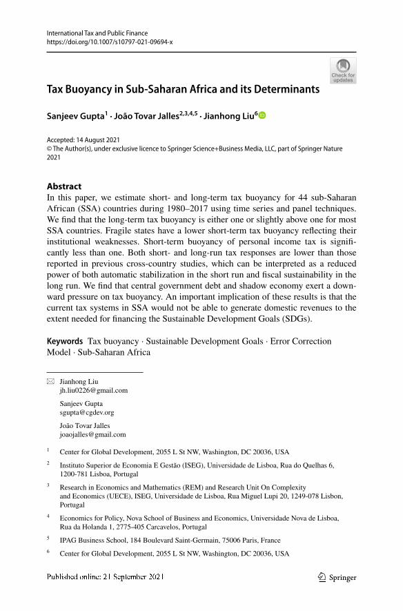
The overall nominal tax revenue and GDP growth for SSA countries are dis-played in Fig. 1. In general, nominal revenues seem to have grown faster than nominal GDP. This suggests that on average, tax buoyancy has been greater than
0
5
10
15
20
25
30
35
40
45
1981 1985 1989 1993 1997 2001 2005 2009 2013 2017
Nominal GDP Nominal Tax Revenue
Fig. 1 Growth in Nominal GDP and Nominal Tax Revenues (%) in Sub-Saharan Africa, 1981–2017. Note: South Sudan, Angola and Democratic Republic of the Congo are excluded due to data non-availa-bility, and result remains unchanged if we exclude Nigeria and South Africa Source: International Centre for Tax and Development (ICTD)’s Government Revenue Dataset
0
10
20
30
40
50
60
70
1981
1983
1985
1987
1989
1991
1993
1995
1997
1999
2001
2003
2005
2007
2009
2011
2013
2015
2017
GDP PIT
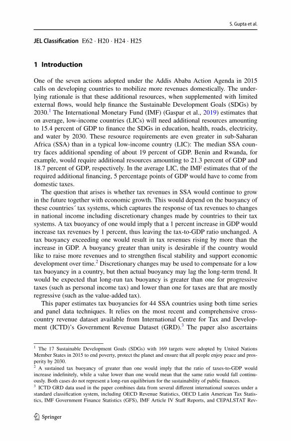
Fig. 2 Growth in Nominal GDP and Personal Income Tax (PIT) (%) in Sub-Saharan Africa, 1981–2017
enue Statistics in Latin America, leading to gains in both coverage and accuracy compared to any other single source. The GRD is available from www. ictd. ac as a Microsoft Excel Spreadsheet (.xls), Open Document Spreadsheet (.ods), or Stata data file (.dta).
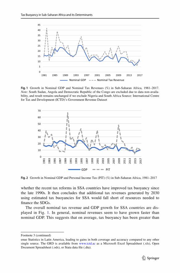
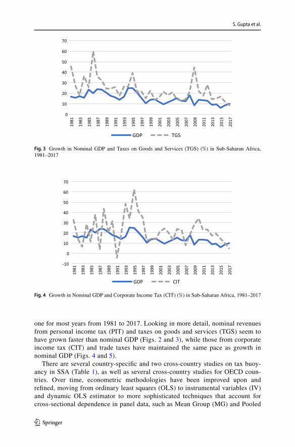
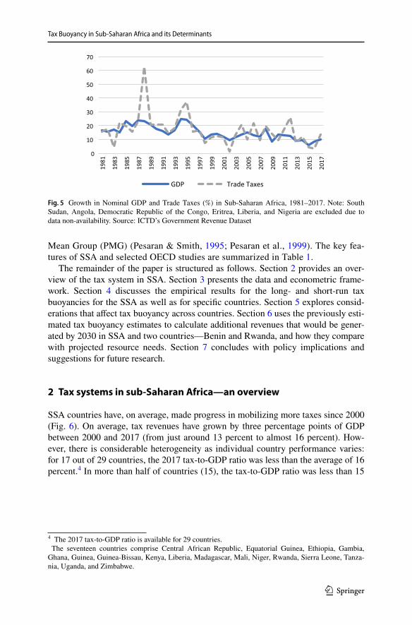
one for most years from 1981 to 2017. Looking in more detail, nominal revenues from personal income tax (PIT) and taxes on goods and services (TGS) seem to have grown faster than nominal GDP (Figs. 2 and 3), while those from corporate income tax (CIT) and trade taxes have maintained the same pace as growth in nominal GDP (Figs. 4 and 5).
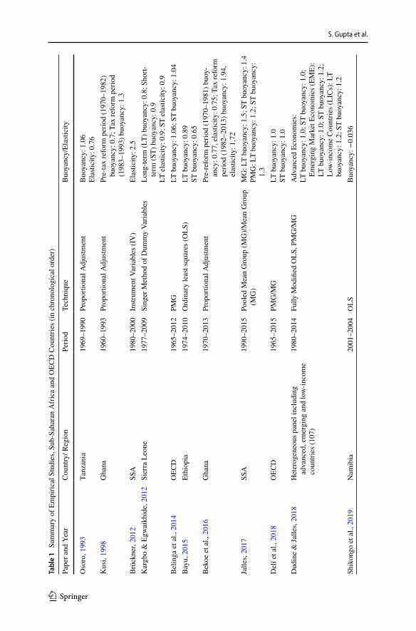
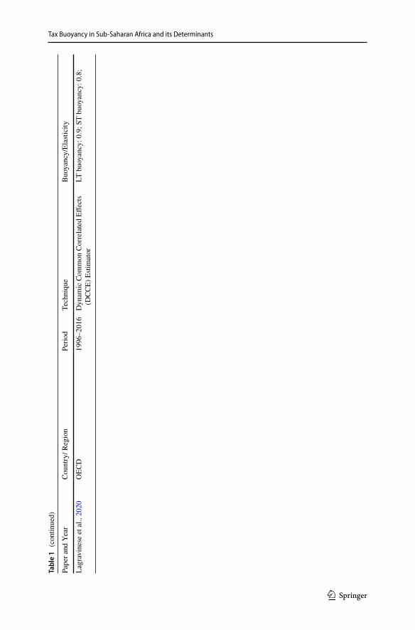
There are several country-specific and two cross-country studies on tax buoy-ancy in SSA (Table 1), as well as several cross-country studies for OECD coun-tries. Over time, econometric methodologies have been improved upon and refined, moving from ordinary least squares (OLS) to instrumental variables (IV) and dynamic OLS estimator to more sophisticated techniques that account for cross-sectional dependence in panel data, such as Mean Group (MG) and Pooled
0
10
20
30
40
50
60
70
1981
1983
1985
1987
1989
1991
1993
1995
1997
1999
2001
2003
2005
2007
2009
2011
2013
2015
2017
GDP TGS
Fig. 3 Growth in Nominal GDP and Taxes on Goods and Services (TGS) (%) in Sub-Saharan Africa, 1981–2017
-10
0
10
20
30
40
50
60
70
1981
1983
1985
1987
1989
1991
1993
1995
1997
1999
2001
2003
2005
2007
2009
2011
2013
2015
2017
GDP CIT
Fig. 4 Growth in Nominal GDP and Corporate Income Tax (CIT) (%) in Sub-Saharan Africa, 1981–2017
1 3
Tax Buoyancy in Sub-Saharan Africa and its Determinants
Mean Group (PMG) (Pesaran & Smith, 1995; Pesaran et al., 1999). The key fea-tures of SSA and selected OECD studies are summarized in Table 1.
The remainder of the paper is structured as follows. Section 2 provides an over-view of the tax system in SSA. Section 3 presents the data and econometric frame-work. Section 4 discusses the empirical results for the long- and short-run tax buoyancies for the SSA as well as for specific countries. Section 5 explores consid-erations that affect tax buoyancy across countries. Section 6 uses the previously esti-mated tax buoyancy estimates to calculate additional revenues that would be gener-ated by 2030 in SSA and two countries—Benin and Rwanda, and how they compare with projected resource needs. Section 7 concludes with policy implications and suggestions for future research.
2 Tax systems in sub‑Saharan Africa—an overview
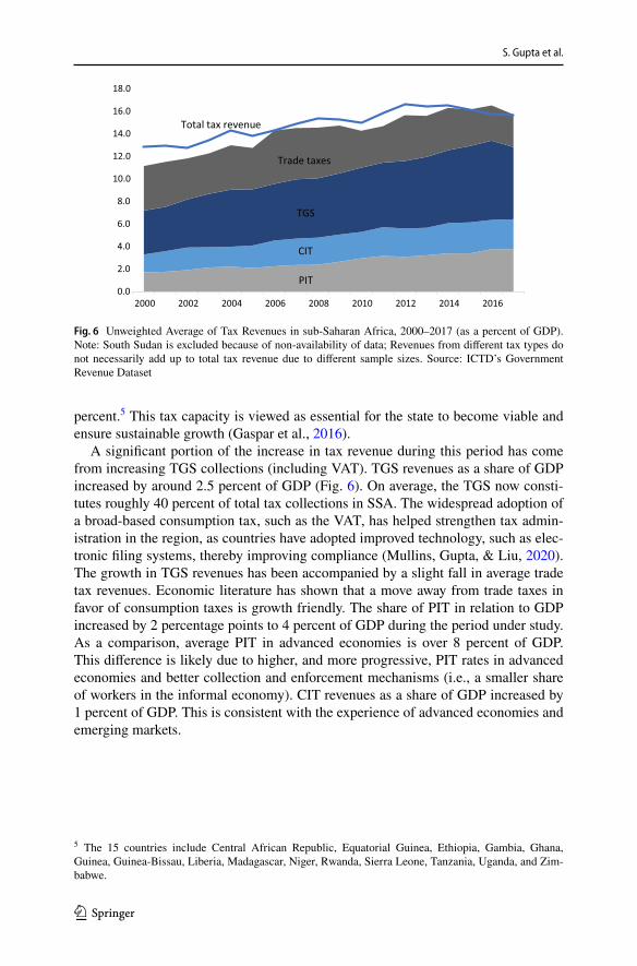
SSA countries have, on average, made progress in mobilizing more taxes since 2000 (Fig. 6). On average, tax revenues have grown by three percentage points of GDP between 2000 and 2017 (from just around 13 percent to almost 16 percent). How-ever, there is considerable heterogeneity as individual country performance varies: for 17 out of 29 countries, the 2017 tax-to-GDP ratio was less than the average of 16 percent.4 In more than half of countries (15), the tax-to-GDP ratio was less than 15
0
10
20
30
40
50
60
70
1981
1983
1985
1987
1989
1991
1993
1995
1997
1999
2001
2003
2005
2007
2009
2011
2013
2015
2017
GDP Trade Taxes
Fig. 5 Growth in Nominal GDP and Trade Taxes (%) in Sub-Saharan Africa, 1981–2017. Note: South Sudan, Angola, Democratic Republic of the Congo, Eritrea, Liberia, and Nigeria are excluded due to data non-availability. Source: ICTD’s Government Revenue Dataset
4 The 2017 tax-to-GDP ratio is available for 29 countries. The seventeen countries comprise Central African Republic, Equatorial Guinea, Ethiopia, Gambia, Ghana, Guinea, Guinea-Bissau, Kenya, Liberia, Madagascar, Mali, Niger, Rwanda, Sierra Leone, Tanza-nia, Uganda, and Zimbabwe.
S. Gupta et al.
1 3
Tabl
e 1
Sum
mar
y of
Em
piric
al S
tudi
es, S
ub-S
ahar
an A
fric
a an
d O
ECD
Cou
ntrie
s (in
chr
onol
ogic
al o
rder
)
Pape
r and
Yea
rC
ount
ry/ R
egio
nPe
riod
Tech
niqu
eB
uoya
ncy/
Elas
ticity
Oso
ro, 1
993
Tanz
ania
1969
–199
0Pr
opor
tiona
l Adj
ustm
ent
Buo
yanc
y: 1
.06
Elas
ticity
: 0.7
6K
usi,
1998
Gha
na19
60–1
993
Prop
ortio
nal A
djus
tmen
tPr
e-ta
x re
form
per
iod
(197
0–19
82)
buoy
ancy
: 0.7
; Tax
refo
rm p
erio
d (1
983–
1993
) buo
yanc
y: 1
.3B
rück
ner,
2012
SSA
1980
–200
0In
strum
ent V
aria
bles
(IV
)El
astic
ity: 2
.5K
argb
o &
Egw
aikh
ide,
201
2Si
erra
Leo
ne19
77–2
009
Sing
er M
etho
d of
Dum
my
Varia
bles
Long
-term
(LT)
buo
yanc
y: 0
.8; S
hort-
term
(ST)
buo
yanc
y: 0
.9LT
ela
stici
ty: 0
.9; S
T el
astic
ity: 0
.9B
elin
ga e
t al.,
201
4O
ECD
1965
–201
2PM
GLT
buo
yanc
y: 1
.06;
ST
buoy
ancy
: 1.0
4B
ayu,
201
5Et
hiop
ia19
74–2
010
Ord
inar
y le
ast s
quar
es (O
LS)
LT b
uoya
ncy:
0.8
9ST
buo
yanc
y: 0
.65
Bek
oe e
t al.,
201
6G
hana
1970
–201
3Pr
opor
tiona
l Adj
ustm
ent
Pre-
refo
rm p
erio
d (1
970–
1981
) buo
y-an
cy: 0
.77,
ela
stici
ty: 0
.75;
Tax
refo
rm
perio
d (1
982–
2013
) buo
yanc
y: 1
.94,
el
astic
ity: 1
.72
Jalle
s, 20
17SS
A19
90–2
015
Pool
ed M
ean
Gro
up (M
G)/M
ean
Gro
up
(MG
)M
G: L
T bu
oyan
cy: 1
.5; S
T bu
oyan
cy: 1
.4PM
G: L
T bu
oyan
cy: 1
.2; S
T bu
oyan
cy:
1.3
Del
i et a
l., 2
018
OEC
D19
65–2
015
PMG
/MG
LT b
uoya
ncy:
1.0
ST b
uoya
ncy:
1.0
Dud
ine
& Ja
lles,
2018
Het
erog
eneo
us p
anel
incl
udin
g ad
vanc
ed, e
mer
ging
and
low
-inco
me
coun
tries
(107
)
1980
–201
4Fu
lly M
odifi
ed O
LS, P
MG
/MG
Adv
ance
d Ec
onom
ies:
LT b
uoya
ncy:
1.0
; ST
buoy
ancy
: 1.0
; Em
ergi
ng M
arke
t Eco
nom
ies (
EME)
: LT
buo
yanc
y: 1
.0; S
T bu
oyan
cy: 1
.2;
Low
-inco
me
Cou
ntrie
s (LI
Cs)
: LT
buoy
ancy
: 1.2
; ST
buoy
ancy
: 1.2
Shik
ongo
et a
l., 2
019
Nam
ibia
2001
–200
4O
LSB
uoya
ncy:
−0.
036
1 3
Tax Buoyancy in Sub-Saharan Africa and its Determinants
Tabl
e 1
(con
tinue
d)
Pape
r and
Yea
rC
ount
ry/ R
egio
nPe
riod
Tech
niqu
eB
uoya
ncy/
Elas
ticity
Lagr
avin
ese
et a
l., 2
020
OEC
D19
96–2
016
Dyn
amic
Com
mon
Cor
rela
ted
Effec
ts
(DC
CE)
Esti
mat
orLT
buo
yanc
y: 0
.9; S
T bu
oyan
cy: 0
.8;
S. Gupta et al.
1 3
percent.5 This tax capacity is viewed as essential for the state to become viable and ensure sustainable growth (Gaspar et al., 2016).
A significant portion of the increase in tax revenue during this period has come from increasing TGS collections (including VAT). TGS revenues as a share of GDP increased by around 2.5 percent of GDP (Fig. 6). On average, the TGS now consti-tutes roughly 40 percent of total tax collections in SSA. The widespread adoption of a broad-based consumption tax, such as the VAT, has helped strengthen tax admin-istration in the region, as countries have adopted improved technology, such as elec-tronic filing systems, thereby improving compliance (Mullins, Gupta, & Liu, 2020). The growth in TGS revenues has been accompanied by a slight fall in average trade tax revenues. Economic literature has shown that a move away from trade taxes in favor of consumption taxes is growth friendly. The share of PIT in relation to GDP increased by 2 percentage points to 4 percent of GDP during the period under study. As a comparison, average PIT in advanced economies is over 8 percent of GDP. This difference is likely due to higher, and more progressive, PIT rates in advanced economies and better collection and enforcement mechanisms (i.e., a smaller share of workers in the informal economy). CIT revenues as a share of GDP increased by 1 percent of GDP. This is consistent with the experience of advanced economies and emerging markets.
0.0
2.0
4.0
6.0
8.0
10.0
12.0
14.0
16.0
18.0
2000 2002 2004 2006 2008 2010 2012 2014 2016
PIT
CIT
TGS
Trade taxes
Total tax revenue
Fig. 6 Unweighted Average of Tax Revenues in sub-Saharan Africa, 2000–2017 (as a percent of GDP). Note: South Sudan is excluded because of non-availability of data; Revenues from different tax types do not necessarily add up to total tax revenue due to different sample sizes. Source: ICTD’s Government Revenue Dataset
5 The 15 countries include Central African Republic, Equatorial Guinea, Ethiopia, Gambia, Ghana, Guinea, Guinea-Bissau, Liberia, Madagascar, Niger, Rwanda, Sierra Leone, Tanzania, Uganda, and Zim-babwe.
1 3
Tax Buoyancy in Sub-Saharan Africa and its Determinants
3 Data and econometric framework
3.1 Data
As explained on page 3 and footnote 7, data for tax revenues come from the Govern-ment Revenue Dataset as compiled by ICTD for 44 sub-Saharan African countries for the period 1980 to 2017.6 This time period includes the most severe financial and economic crises in many decades, extending between 2007 and 2013. The global financial crisis stressed the tax systems of SSA countries. In addition to buoyancy of aggregate tax revenues, we also focus on four tax categories, namely personal income tax (PIT), corporate income tax (CIT), tax on goods and services (TGS), and trade taxes. Disaggregated data by tax types are available for a smaller number of countries and are of shorter duration. Data on tax revenues are expressed in real terms in local currency units.
3.2 Empirical framework
We specify an autoregressive distributed lag (ARDL) model which is used to ana-lyze dynamic relationships with time-series data in a single-equation framework shown in Eq. (1). The ARDL model considers both levels and changes of the rele-vant variables in order to identify both the long-run growth and short-run variability of tax revenues through a single equation:
Taxi,t denotes tax revenue in country i in year t, GDPi,t stands for its level of GDP, �i is the country-specific effect and �it is the error term—both the tax variables and GDP are expressed in logs.
We follow the existing literature (Belinga et al., 2014; Deli et al., 2018; Dudine & Jalles, 2018) and use the optimal lag length to be equal to 1 for both p and q in Eq. (1), which gives us Eq. (2).7 It suggests that developments in tax revenue can be explained by GDP of the current and preceding period, and by tax revenue in the preceding period.
Equation (2) can be transformed into a single error correction model (ECM) of Eq. (3), which shows that changes in tax can be explained by changes in GDP and corrections made in response to the disequilibrium from last period given in the parenthesis.
6 South Sudan is excluded because of non-availability of sufficiently long time series.7 We also extended the lag length to p = q = 2. Results are shown in the Appendix Table 13.
S. Gupta et al.
1 3
where �i measures the instantaneous effect of a change in GDP on tax revenue, reflecting the short-term buoyancy of the tax. The parameter �i denotes the long-term buoyancy. The parameter �i measures the speed of adjustment, i.e., how fast the system converges to its long-run equilibrium. Application of the error correction model presupposes that tax revenues and GDP are cointegrated. Before estimating Eq. (3), it is thus essential to diagnose both the stationarity and cointegration prop-erties of the different time series.
We follow a two-step empirical strategy in estimating Eq. (3). In the first step, we apply time series techniques to estimate short- and long-term tax buoyancy for SSA countries with adequate data (that is, applying these to those countries with a rea-sonably continuous set of observations for the variables of interest). As some coun-tries lacked ample data or failed to pass the necessary statistical test, we resorted to the application of panel techniques in the next step. This allowed us to maximize the cross-sectional and time series dimensions and to make use of all available data in estimating tax buoyancy of SSA as a region, which is not possible with time series techniques.
4 Empirical results
4.1 Time series regressions
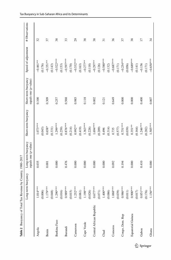
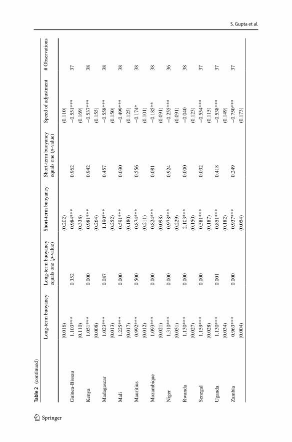
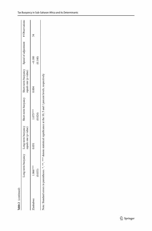
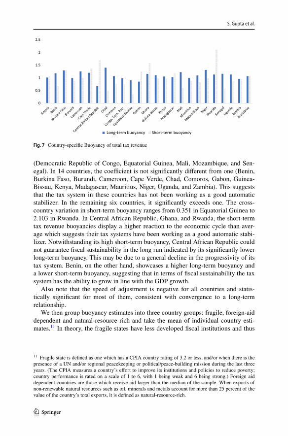
For individual countries, we estimate short- and long-term buoyancy for total tax revenues by using time series techniques provided taxes and GDP are found to be cointegrated.8Since sufficiently long disaggregated data on specific tax types are not available, we skip time series estimates for them. We then test whether the long- and short-term buoyancy equals one. Table 2 and Fig. 7 display the estimates for 25 out of 44 SSA countries which passed the cointegration test.9 Estimates for the remain-ing 19 countries are available from authors upon request.10
Results suggest an average long-term buoyancy of 1.088. It is significantly smaller than one in three countries (Central African Republic, Equatorial Guinea and Zambia). In five countries (Burundi, Democratic Republic of Congo, Gabon, Guinea-Bissau and Mauritius), the coefficient is not significantly different from one, which means for these eight countries, tax revenue is not growing faster than GDP growth. In the remaining 17 countries, it exceeds one by a small margin.
Results also suggest an average short-term buoyancy of 1.004 which is smaller than the long-term buoyancy. It is significantly smaller than one in 5 countries
(3)ΔlnTaxi,t = �i(
lnTaxi,t−1 − �ilnGDPi,t−1)
+ �iΔlnGDPi,t + �i + �it
8 Results of country specific cointegration tests are available from the authors upon request.9 The Newey–West estimator is applied to account for autocorrelation and heteroskedasticity in the error terms.10 We excluded South Sudan because of non-availability of data. The failure to pass the cointegration tests in 19 countries is probably a reflection of structural changes taking place in these countries.
1 3
Tax Buoyancy in Sub-Saharan Africa and its Determinants
Tabl
e 2
Buo
yanc
y of
Tot
al T
ax R
even
ue b
y C
ount
ry, 1
980–
2017
Long
-term
buo
yanc
yLo
ng-te
rm b
uoya
ncy
equa
ls o
ne (p
-val
ue)
Shor
t-ter
m b
uoya
ncy
Shor
t-ter
m b
uoya
ncy
equa
ls o
ne (p
-val
ue)
Spee
d of
adj
ustm
ent
# O
bser
vatio
ns
Ang
ola
1.01
4***
0.03
51.
073*
**0.
100
−0.
461*
*32
(0.0
06)
(0.0
43)
(0.1
76)
Ben
in1.
179*
**0.
001
0.65
8*0.
309
−0.
351*
*37
(0.0
48)
(0.3
31)
(0.1
43)
Bur
kina
Fas
o1.
290*
**0.
000
1.29
9***
0.25
7−
0.52
2***
38(0
.016
)(0
.259
)(0
.153
)B
urun
di0.
989*
**0.
476
0.87
6***
0.56
8−
0.59
7***
33(0
.015
)(0
.214
)(0
.170
)C
amer
oon
1.25
2***
0.00
00.
992*
*0.
985
−0.
532*
**29
(0.0
61)
(0.4
19)
(0.1
63)
Cap
e Ve
rde
1.19
8***
0.00
01.
363*
**0.
118
−0.
277*
*38
(0.0
26)
(0.2
26)
(0.1
18)
Cen
tral A
fric
an R
epub
lic0.
677*
**0.
000
1.69
4***
0.00
2−
0.29
7**
38(0
.071
)(0
.209
)(0
.126
)C
had
1.40
0***
0.00
00.
496
0.12
1−
0.58
0***
31(0
.086
)(0
.314
)(0
.132
)C
omor
os1.
068*
**0.
092
0.73
50.
649
−0.
687*
**36
(0.0
39)
(0.5
77)
(0.1
71)
Con
go, D
em. R
ep0.
986*
**0.
194
0.75
1***
0.00
0−
0.25
4***
37(0
.011
)(0
.039
)(0
.056
)Eq
uato
rial G
uine
a0.
900*
**0.
000
0.35
1**
0.00
0−
0.68
9***
38(0
.017
)(0
.164
)(0
.141
)G
abon
0.85
1***
0.41
01.
246*
**0.
400
−0.
156
17(0
.176
)(0
.282
)(0
.171
)G
hana
1.15
6***
0.00
01.
585*
**0.
007
−0.
650*
**34
S. Gupta et al.
1 3
Tabl
e 2
(con
tinue
d)
Long
-term
buo
yanc
yLo
ng-te
rm b
uoya
ncy
equa
ls o
ne (p
-val
ue)
Shor
t-ter
m b
uoya
ncy
Shor
t-ter
m b
uoya
ncy
equa
ls o
ne (p
-val
ue)
Spee
d of
adj
ustm
ent
# O
bser
vatio
ns
(0.0
16)
(0.2
02)
(0.1
10)
Gui
nea-
Bis
sau
1.10
3***
0.35
20.
984*
**0.
962
−0.
551*
**37
(0.1
10)
(0.3
38)
(0.1
69)
Ken
ya1.
051*
**0.
000
0.98
1***
0.94
2−
0.53
7***
38(0
.008
)(0
.264
)(0
.155
)M
adag
asca
r1.
023*
**0.
087
1.19
0***
0.45
7−
0.55
8***
38(0
.013
)(0
.252
)(0
.150
)M
ali
1.22
5***
0.00
00.
591*
**0.
030
−0.
499*
**38
(0.0
17)
(0.1
80)
(0.1
25)
Mau
ritiu
s0.
992*
**0.
500
0.87
4***
0.55
6−
0.17
4*38
(0.0
12)
(0.2
11)
(0.1
01)
Moz
ambi
que
1.09
3***
0.00
00.
824*
**0.
081
−0.
185*
*38
(0.0
21)
(0.0
98)
(0.0
91)
Nig
er1.
310*
**0.
000
0.97
8***
0.92
4−
0.25
5***
36(0
.051
)(0
.229
)(0
.091
)R
wan
da1.
130*
**0.
000
2.10
3***
0.00
0−
0.04
038
(0.0
27)
(0.1
50)
(0.1
23)
Sene
gal
1.15
9***
0.00
00.
581*
**0.
032
−0.
554*
**37
(0.0
28)
(0.1
87)
(0.1
15)
Uga
nda
1.13
0***
0.00
10.
851*
**0.
418
−0.
538*
**37
(0.0
34)
(0.1
82)
(0.1
49)
Zam
bia
0.96
3***
0.00
00.
937*
**0.
249
−0.
750*
**37
(0.0
04)
(0.0
54)
(0.1
73)
1 3
Tax Buoyancy in Sub-Saharan Africa and its Determinants
Tabl
e 2
(con
tinue
d)
Long
-term
buo
yanc
yLo
ng-te
rm b
uoya
ncy
equa
ls o
ne (p
-val
ue)
Shor
t-ter
m b
uoya
ncy
Shor
t-ter
m b
uoya
ncy
equa
ls o
ne (p
-val
ue)
Spee
d of
adj
ustm
ent
# O
bser
vatio
ns
Zim
babw
e1.
066*
**0.
051
1.07
5***
0.00
4−
0.18
034
(0.0
33)
(0.0
24)
(0.1
40)
Not
e: S
tand
ard
erro
rs in
par
enth
eses
. *, *
*, *
** d
enot
e st
atist
ical
sign
ifica
nce
at th
e 10
, 5 a
nd 1
per
cent
leve
ls, r
espe
ctiv
ely
S. Gupta et al.
1 3
(Democratic Republic of Congo, Equatorial Guinea, Mali, Mozambique, and Sen-egal). In 14 countries, the coefficient is not significantly different from one (Benin, Burkina Faso, Burundi, Cameroon, Cape Verde, Chad, Comoros, Gabon, Guinea-Bissau, Kenya, Madagascar, Mauritius, Niger, Uganda, and Zambia). This suggests that the tax system in these countries has not been working as a good automatic stabilizer. In the remaining six countries, it significantly exceeds one. The cross-country variation in short-term buoyancy ranges from 0.351 in Equatorial Guinea to 2.103 in Rwanda. In Central African Republic, Ghana, and Rwanda, the short-term tax revenue buoyancies display a higher reaction to the economic cycle than aver-age which suggests their tax systems have been working as a good automatic stabi-lizer. Notwithstanding its high short-term buoyancy, Central African Republic could not guarantee fiscal sustainability in the long run indicated by its significantly lower long-term buoyancy. This may be due to a general decline in the progressivity of its tax system. Benin, on the other hand, showcases a higher long-term buoyancy and a lower short-term buoyancy, suggesting that in terms of fiscal sustainability the tax system has the ability to grow in line with the GDP growth.
Also note that the speed of adjustment is negative for all countries and statis-tically significant for most of them, consistent with convergence to a long-term relationship.
We then group buoyancy estimates into three country groups: fragile, foreign-aid dependent and natural-resource rich and take the mean of individual country esti-mates.11 In theory, the fragile states have less developed fiscal institutions and thus
0
0.5
1
1.5
2
2.5
Long-term buoyancy Short-term buoyancy
Fig. 7 Country-specific Buoyancy of total tax revenue
11 Fragile state is defined as one which has a CPIA country rating of 3.2 or less, and/or when there is the presence of a UN and/or regional peacekeeping or political/peace-building mission during the last three years. (The CPIA measures a country’s effort to improve its institutions and policies to reduce poverty; country performance is rated on a scale of 1 to 6, with 1 being weak and 6 being strong.) Foreign aid dependent countries are those which receive aid larger than the median of the sample. When exports of non-renewable natural resources such as oil, minerals and metals account for more than 25 percent of the value of the country’s total exports, it is defined as natural-resource-rich.
1 3
Tax Buoyancy in Sub-Saharan Africa and its Determinants
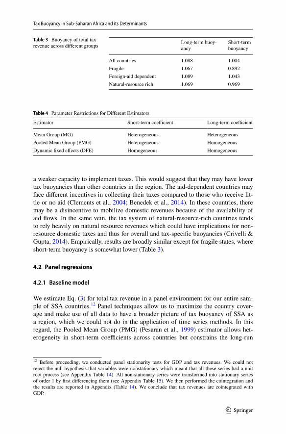
a weaker capacity to implement taxes. This would suggest that they may have lower tax buoyancies than other countries in the region. The aid-dependent countries may face different incentives in collecting their taxes compared to those who receive lit-tle or no aid (Clements et al., 2004; Benedek et al., 2014). In these countries, there may be a disincentive to mobilize domestic revenues because of the availability of aid flows. In the same vein, the tax system of natural-resource-rich countries tends to rely heavily on natural resource revenues which could have implications for non-resource domestic taxes and thus for overall and tax-specific buoyancies (Crivelli & Gupta, 2014). Empirically, results are broadly similar except for fragile states, where short-term buoyancy is somewhat lower (Table 3).
4.2 Panel regressions
4.2.1 Baseline model
We estimate Eq. (3) for total tax revenue in a panel environment for our entire sam-ple of SSA countries.12 Panel techniques allow us to maximize the country cover-age and make use of all data to have a broader picture of tax buoyancy of SSA as a region, which we could not do in the application of time series methods. In this regard, the Pooled Mean Group (PMG) (Pesaran et al., 1999) estimator allows het-erogeneity in short-term coefficients across countries but constrains the long-run
Table 3 Buoyancy of total tax revenue across different groups
Long-term buoy-ancy
Short-term buoyancy
All countries 1.088 1.004Fragile 1.067 0.892Foreign-aid dependent 1.089 1.043Natural-resource rich 1.069 0.969
Table 4 Parameter Restrictions for Different Estimators
Mean Group (MG) Heterogeneous HeterogeneousPooled Mean Group (PMG) Heterogeneous HomogeneousDynamic fixed effects (DFE) Homogeneous Homogeneous
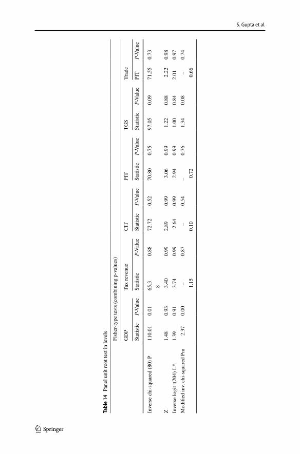
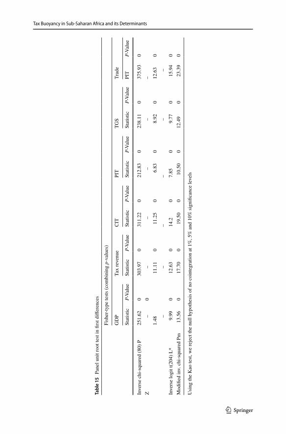
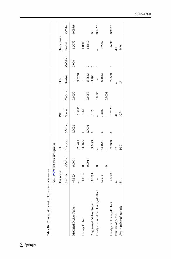
12 Before proceeding, we conducted panel stationarity tests for GDP and tax revenues. We could not reject the null hypothesis that variables were nonstationary which meant that all these series had a unit root process (see Appendix Table 14). All non-stationary series were transformed into stationary series of order 1 by first differencing them (see Appendix Table 15). We then performed the cointegration and the results are reported in Appendix (Table 14). We conclude that tax revenues are cointegrated with GDP.
S. Gupta et al.
1 3
coefficients to be equal. That is, it assumes that the long-term relationship between dependent and independent variables is the same across countries. The Mean Group (MG) (Pesaran & Smith, 1995) estimator, in contrast, allows for full parameter het-erogeneity; that is, a separate regression is estimated for each country and an aver-age reported. Both MG and PMG are appropriate for the analysis of dynamic pan-els with both large time and cross section dimensions, and they have the advantage of accommodating both the long-run equilibrium and the possibly heterogeneous dynamic adjustment process. At the other end of the scale, dynamic fixed effects estimation constrains all short-run and long-run coefficients to be equal across coun-tries (see Table 4 for a summary).
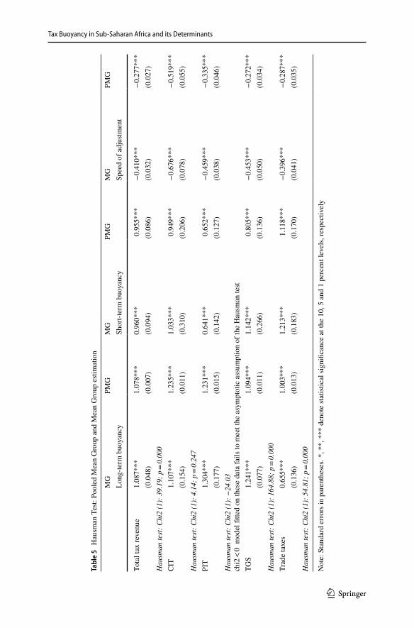
To test the validity of the assumption that the long-run relationship between the growth of GDP and tax revenues is the same across countries, we performed the Hausman test to compare the resulting PMG estimates against those stemming from MG estimator.13 Table 5 displays the estimated coefficients using a full panel of 40 SSA countries14 for long-term, short-term and the speed of adjustment using both PMG and MG and the resulting Hausman test statistics. For CIT, the PMG procedure produces estimates that are consistent and more efficient and, thus, it is preferred. MG estimator is preferred for remainder of tax components and total tax revenue. Furthermore, coefficient estimates for total tax revenue and PIT under both PMG and MG are broadly similar.
We find that the long-term buoyancy for total tax revenue and most tax com-ponents is higher than one, which suggests that most of the levies are progressive, except for trade taxes. Estimates of CIT buoyancies are in the same range as those of the OECD countries. The short-term buoyancy is generally lower, and in one case, PIT, it is significantly lower than one. One possible reason can be wage rigidity in the formal sector. However, for trade taxes, short-term buoyancy is significantly higher than long-term buoyancy. The speed of adjustment for trade taxes is the low-est among all taxes, i.e., speed of adjustment toward its long-term equilibrium is relatively slow.
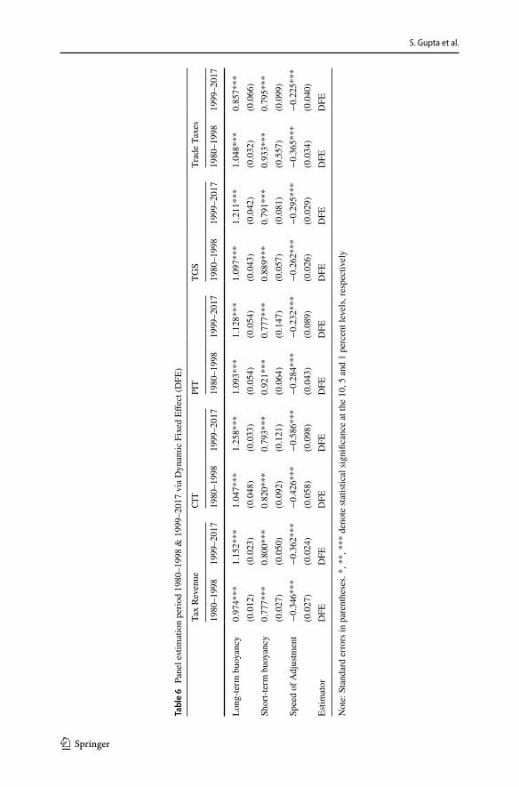
We further studied whether tax buoyancies have changed over time in sub-Saha-ran Africa against the background of tax reforms introduced by many countries since the late 1990s. Consequently, we divided our sample evenly into two periods, 1980–1998 and 1999–2017.15 This way we get the largest number of observations for each time segment which allows us to apply dynamic fixed effects estimation.
13 We follow the same approach as used by McNabb (2018). Hausman test evaluates the consistency of an estimator when compared to an alternative, less efficient estimator which is already known to be consistent. Here in our case, under the null hypothesis, both estimators (MG and PMG) are consistent, but PMG is efficient. If we reject the null hypothesis, it means that PMG is inconsistent, and MG is pre-ferred. Otherwise, PMG is preferred.14 To make the panel more balanced, we drop 4 countries in our sample.15 Ideally, we would have liked to identify years with a dummy when tax reforms were implemented in SSA. Unfortunately, such data are not available. The one that exists for 45 emerging and low-income countries covers only 12 countries in SSA and that too for 2000–2015 period (Akitoby et al., 2019). This left us with an imperfect means of dividing the sample into two segments to capture the impact of tax reforms in recent years. Since the bulk of major tax policy changes in SSA countries were initiated in 1990s (Gillis, 2001), the post-1999 period captures their impact on tax buoyancy.
1 3
Tax Buoyancy in Sub-Saharan Africa and its Determinants
Tabl
e 5
Hau
sman
Tes
t: Po
oled
Mea
n G
roup
and
Mea
n G
roup
esti
mat
ion
Not
e: S
tand
ard
erro
rs in
par
enth
eses
. *, *
*, *
** d
enot
e st
atist
ical
sign
ifica
nce
at th
e 10
, 5 a
nd 1
per
cent
leve
ls, r
espe
ctiv
ely
MG
PMG
MG
PMG
MG
PMG
Long
-term
buo
yanc
ySh
ort-t
erm
buo
yanc
ySp
eed
of a
djus
tmen
t
Tota
l tax
reve
nue
1.08
7***
1.07
8***
0.96
0***
0.95
5***
−0.
410*
**−
0.27
7***
(0.0
48)
(0.0
07)
(0.0
94)
(0.0
86)
(0.0
32)
(0.0
27)
Hau
sman
test
: Chi
2 (1
): 3
9.19
; p =
0.00
0C
IT1.
107*
**1.
235*
**1.
033*
**0.
949*
**−
0.67
6***
−0.
519*
**(0
.154
)(0
.011
)(0
.310
)(0
.206
)(0
.078
)(0
.055
)H
ausm
an te
st: C
hi2
(1):
4.1
4; p
= 0.
247
PIT
1.30
4***
1.23
1***
0.64
1***
0.65
2***
−0.
459*
**−
0.33
5***
(0.1
77)
(0.0
15)
(0.1
42)
(0.1
27)
(0.0
38)
(0.0
46)
Hau
sman
test
: Chi
2 (1
): −
24.0
3ch
i2 <
0 m
odel
fitte
d on
thes
e da
ta fa
ils to
mee
t the
asy
mpt
otic
ass
umpt
ion
of th
e H
ausm
an te
stTG
S1.
241*
**1.
094*
**1.
142*
**0.
805*
**−
0.45
3***
−0.
272*
**(0
.077
)(0
.011
)(0
.266
)(0
.136
)(0
.050
)(0
.034
)H
ausm
an te
st: C
hi2
(1):
164
.88;
p =
0.00
0Tr
ade
taxe
s0.
655*
**1.
003*
**1.
213*
**1.
118*
**−
0.39
6***
−0.
287*
**(0
.136
)(0
.013
)(0
.183
)(0
.170
)(0
.041
)(0
.035
)H
ausm
an te
st: C
hi2
(1):
54.
81; p
= 0.
000
S. Gupta et al.
1 3
Tabl
e 6
Pan
el e
stim
atio
n pe
riod
1980
–199
8 &
199
9–20
17 v
ia D
ynam
ic F
ixed
Effe
ct (D
FE)
Not
e: S
tand
ard
erro
rs in
par
enth
eses
. *, *
*, *
** d
enot
e st
atist
ical
sign
ifica
nce
at th
e 10
, 5 a
nd 1
per
cent
leve
ls, r
espe
ctiv
ely
Tax
Reve
nue
CIT
PIT
TGS
Trad
e Ta
xes
1980
–199
819
99–2
017
1980
–199
819
99–2
017
1980
–199
819
99–2
017
1980
–199
819
99–2
017
1980
–199
819
99–2
017
Long
-term
buo
yanc
y0.
974*
**1.
152*
**1.
047*
**1.
258*
**1.
093*
**1.
128*
**1.
097*
**1.
211*
**1.
048*
**0.
857*
**(0
.012
)(0
.023
)(0
.048
)(0
.033
)(0
.054
)(0
.054
)(0
.043
)(0
.042
)(0
.032
)(0
.066
)Sh
ort-t
erm
buo
yanc
y0.
777*
**0.
800*
**0.
820*
**0.
793*
**0.
921*
**0.
777*
**0.
889*
**0.
791*
**0.
933*
**0.
795*
**(0
.027
)(0
.050
)(0
.092
)(0
.121
)(0
.064
)(0
.147
)(0
.057
)(0
.081
)(0
.557
)(0
.099
)Sp
eed
of A
djus
tmen
t−
0.34
6***
−0.
362*
**−
0.42
6***
−0.
586*
**−
0.28
4***
−0.
232*
**−
0.26
2***
−0.
295*
**−
0.36
5***
−0.
225*
**(0
.027
)(0
.024
)(0
.058
)(0
.098
)(0
.043
)(0
.089
)(0
.026
)(0
.029
)(0
.034
)(0
.040
)Es
timat
orD
FED
FED
FED
FED
FED
FED
FED
FED
FED
FE
1 3
Tax Buoyancy in Sub-Saharan Africa and its Determinants
If estimates in the latter time period turned out to be higher, it would suggest that tax reforms implemented since 1999 have contributed to enhancing tax buoyancy. Because the resulting two time periods are relatively short, it is not possible to use MG or PMG and we are forced to rely instead on the DFE estimator. Results are displayed in Table 6.
Results suggest that, for overall taxes and most tax components, there is an increase in long-term buoyancy during the 1999–2017 period, except for trade taxes. The latter result is understandable given the declining reliance on trade taxes in SSA countries. Results suggest that structural improvements in tax systems in the second period are indeed having a tangible impact on tax buoyancies.
4.2.2 The role of business cycle
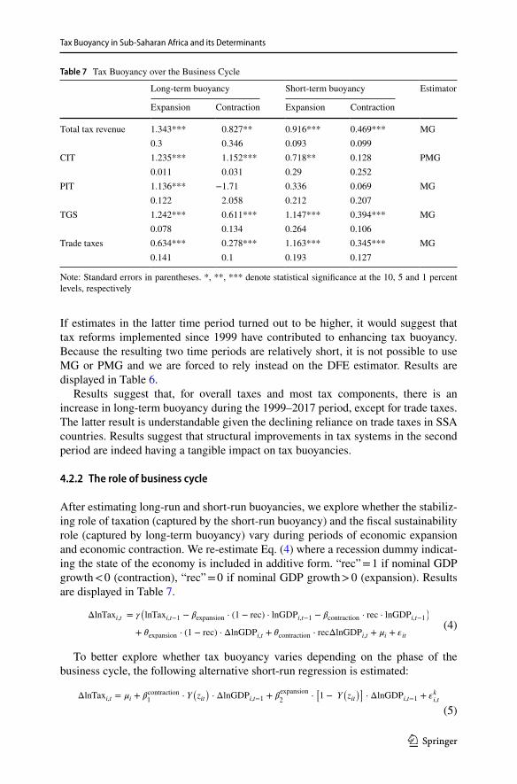
After estimating long-run and short-run buoyancies, we explore whether the stabiliz-ing role of taxation (captured by the short-run buoyancy) and the fiscal sustainability role (captured by long-term buoyancy) vary during periods of economic expansion and economic contraction. We re-estimate Eq. (4) where a recession dummy indicat-ing the state of the economy is included in additive form. “rec” = 1 if nominal GDP growth < 0 (contraction), “rec” = 0 if nominal GDP growth > 0 (expansion). Results are displayed in Table 7.
To better explore whether tax buoyancy varies depending on the phase of the business cycle, the following alternative short-run regression is estimated:
1+exp(−𝛾zit), 𝛾 > 0 where z is an indicator of the state of the economy
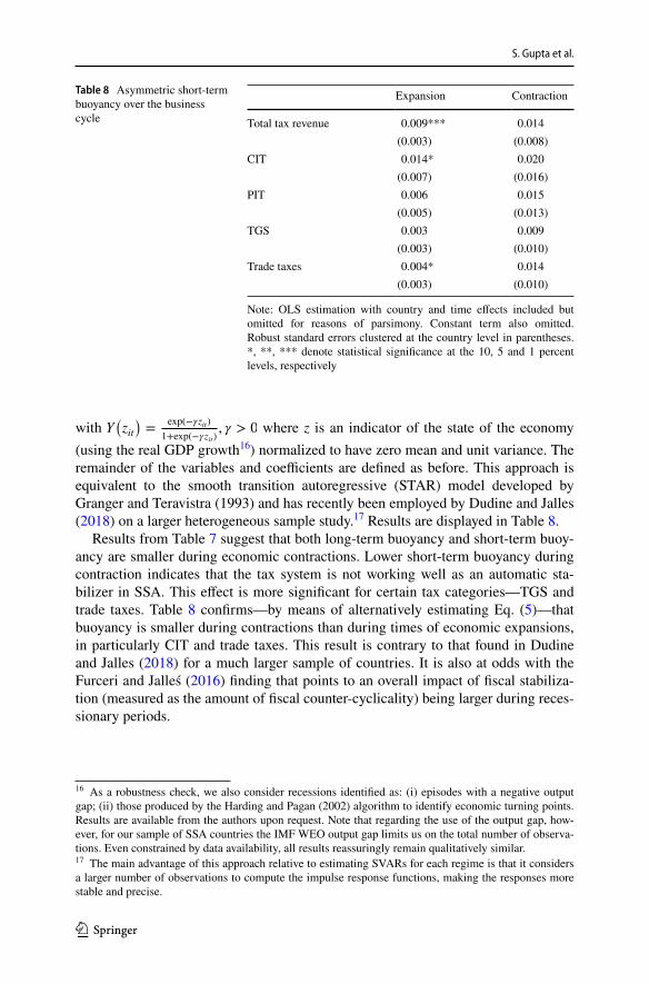
(using the real GDP growth16) normalized to have zero mean and unit variance. The remainder of the variables and coefficients are defined as before. This approach is equivalent to the smooth transition autoregressive (STAR) model developed by Granger and Teravistra (1993) and has recently been employed by Dudine and Jalles (2018) on a larger heterogeneous sample study.17 Results are displayed in Table 8.
Results from Table 7 suggest that both long-term buoyancy and short-term buoy-ancy are smaller during economic contractions. Lower short-term buoyancy during contraction indicates that the tax system is not working well as an automatic sta-bilizer in SSA. This effect is more significant for certain tax categories—TGS and trade taxes. Table 8 confirms—by means of alternatively estimating Eq. (5)—that buoyancy is smaller during contractions than during times of economic expansions, in particularly CIT and trade taxes. This result is contrary to that found in Dudine and Jalles (2018) for a much larger sample of countries. It is also at odds with the Furceri and Jalleś (2016) finding that points to an overall impact of fiscal stabiliza-tion (measured as the amount of fiscal counter-cyclicality) being larger during reces-sionary periods.
Table 8 Asymmetric short-term buoyancy over the business cycle
Note: OLS estimation with country and time effects included but omitted for reasons of parsimony. Constant term also omitted. Robust standard errors clustered at the country level in parentheses. *, **, *** denote statistical significance at the 10, 5 and 1 percent levels, respectively
Expansion Contraction
Total tax revenue 0.009*** 0.014(0.003) (0.008)
CIT 0.014* 0.020(0.007) (0.016)
PIT 0.006 0.015(0.005) (0.013)
TGS 0.003 0.009(0.003) (0.010)
Trade taxes 0.004* 0.014(0.003) (0.010)
16 As a robustness check, we also consider recessions identified as: (i) episodes with a negative output gap; (ii) those produced by the Harding and Pagan (2002) algorithm to identify economic turning points. Results are available from the authors upon request. Note that regarding the use of the output gap, how-ever, for our sample of SSA countries the IMF WEO output gap limits us on the total number of observa-tions. Even constrained by data availability, all results reassuringly remain qualitatively similar.17 The main advantage of this approach relative to estimating SVARs for each regime is that it considers a larger number of observations to compute the impulse response functions, making the responses more stable and precise.
1 3
Tax Buoyancy in Sub-Saharan Africa and its Determinants
Tabl
e 9
Rob
ustn
ess c
heck
: con
trolli
ng fo
r infl
atio
n
Not
e: S
tand
ard
erro
rs in
par
enth
eses
. *, *
*, *
** d
enot
e st
atist
ical
sign
ifica
nce
at th
e 10
, 5 a
nd 1
per
cent
leve
ls, r
espe
ctiv
ely
Tax
Reve
nue
CIT
PIT
TGS
Trad
e Ta
xes
No
cont
rol
Con
trol
No
cont
rol
Con
trol
No
cont
rol
Con
trol
No
cont
rol
Con
trol
No
cont
rol
Con
trol
Long
-term
buo
yanc
y1.
087*
**1.
094*
**1.
235*
**1.
230*
**1.
304*
**1.
309*
**1.
241*
**1.
179*
**0.
655*
**1.
014
(0.0
48)
(0.0
78)
(0.0
11)
(0.0
12)
(0.1
77)
(0.3
12)
(0.0
77)
(0.0
45)
(0.1
36)
(0.7
34)
Shor
t-ter
m b
uoya
ncy
0.96
0***
0.80
6***
0.94
9***
1.06
9***
0.64
1***
0.69
4***
1.14
2***
0.83
9***
1.21
3***
1.06
6***
(0.0
94)
(0.1
24)
(0.2
06)
(0.2
40)
(0.1
42)
(0.2
37)
(0.2
66)
(0.1
44)
(0.1
83)
(0.2
28)
Long
-term
pric
e eff
ect
0.02
00.
000
−0.
090
0.01
3−
0.01
5(0
.012
)(0
.000
)(0
.089
)(0
.010
)(0
.023
)Sh
ort-t
erm
pric
e eff
ect
0.00
2−
0.00
20.
008
0.00
20.
001
(0.0
01)
(0.0
03)
(0.0
05)
(0.0
02)
(0.0
02)
Spee
d of
Adj
ustm
ent
−0.
410*
**−
0.40
3***
−0.
519*
**−
0.37
6***
−0.
459*
**−
0.49
3***
−0.
453*
**−
0.45
5***
−0.
396*
**−
0.38
8***
(0.0
32)
(0.0
34)
(0.0
55)
(0.0
98)
(0.0
38)
(0.0
69)
(0.0
50)
(0.0
41)
(0.0
41)
(0.0
46)
#Cou
ntrie
s40
3937
3640
3940
3740
39#O
bser
vatio
ns1,
349
1,32
878
376
181
880
11,
066
1,04
51,
104
1,09
7Es
timat
orM
GM
GPM
GPM
GM
GM
GM
GM
GM
GM
G
S. Gupta et al.
1 3
4.2.3 Controlling for inflation
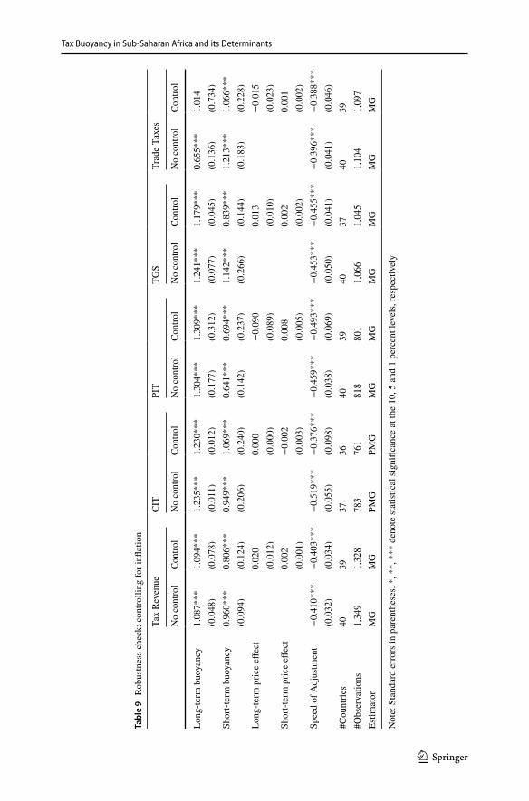
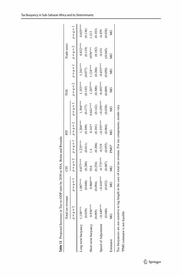
As a robustness check, we also added inflation as a control variable to assess whether tax buoyancy is independent of price changes. If it is, the same relationship would be obtained if real variables were used instead. Results in Table 9 show the coefficients for long-term buoyancy remain unchanged. Hence, long-term tax buoy-ancy appears neutral with respect to inflation, meaning long-term tax buoyancy in real terms is not significantly different from its nominal value. However, the coef-ficients of short-term buoyancy of total tax revenue, TGS and trade taxes are now smaller than before, meaning that tax buoyancy in real terms is smaller than the cor-responding nominal value for these taxes. Short-term tax buoyancy of PIT and CIT remains unchanged.
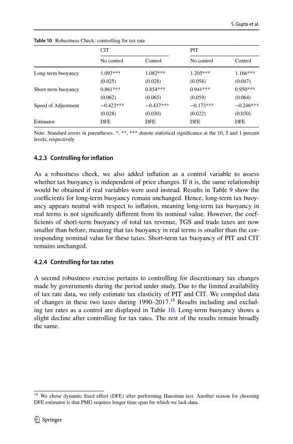
4.2.4 Controlling for tax rates
A second robustness exercise pertains to controlling for discretionary tax changes made by governments during the period under study. Due to the limited availability of tax rate data, we only estimate tax elasticity of PIT and CIT. We compiled data of changes in these two taxes during 1990–2017.18 Results including and exclud-ing tax rates as a control are displayed in Table 10. Long-term buoyancy shows a slight decline after controlling for tax rates. The rest of the results remain broadly the same.
Table 10 Robustness Check: controlling for tax rate
Note: Standard errors in parentheses. *, **, *** denote statistical significance at the 10, 5 and 1 percent levels, respectively
Speed of Adjustment −0.423*** −0.437*** −0.173*** −0.246***(0.028) (0.030) (0.022) (0.030)
Estimator DFE DFE DFE DFE
18 We chose dynamic fixed effect (DFE) after performing Hausman test. Another reason for choosing DFE estimator is that PMG requires longer time span for which we lack data.
1 3
Tax Buoyancy in Sub-Saharan Africa and its Determinants
5 What considerations affect tax buoyancy across countries
In this section, we study the factors that influence cross-country differences in long-term buoyancy. The first variable included in the analysis is the share of value added by agriculture (as a share of GDP). Tanzi and Zee (2000) suggest that a large share of agriculture is associated with a smaller PIT and TGS. The same conclusions were reached by Ahmad and Stern (1991), Teera and Hudson (2004), and Stotsky and Wolde-Mariam (1997). Since agriculture is a difficult sector to tax, we expect a high share of agriculture to be associated with low tax buoyancy. The second variable we consider is the size of shadow economy. Shadow economy comprises economic activity that is undeclared to the tax authorities. An economy with a high share of shadow economy is likely to be associated with low tax buoyancy. The third variable included in our analysis is the size of central government debt as a share of GDP. A high level of debt reflects weak fiscal discipline and concerns about fiscal sustain-ability. It could suggest excessive government spending which does not add to eco-nomic growth. These considerations could adversely impact taxpayers’ incentive to honor their tax obligations (Gupta & Plant, 2019). The fourth variable we test is the prevalence of corruption—defined as the abuse of public office for private gain. A high incidence of corruption reflects weak government institutions. We also include CPIA efficiency of revenue mobilization rating as a proxy for strength of prevailing tax institutions in the country. Finally, we test whether incidence of a conflict affects tax buoyancy.19
We estimate the country-specific average of each indicator and then compute the cross-country median for each country in our sample. We then split the sample between those countries above or below the median and create a dummy variable taking value 1 when the level of the indicator is above the median. Finally, we take the estimated long-term buoyancy coefficients presented in Table 2 as our dependent variable. We estimate the following regression by OLS:
where �̂i is an estimate of the long-term tax buoyancy of country i, �i is constant, �i is the error term. Central government debt, corruption index, share of agriculture in value added, the size of shadow economy, efficiency of revenue mobilization, and conflict are dummy variables created above. �1-�6 are coefficients of interest. Results
+ 𝜑5efficiency of revenue mobilizationi + 𝜑6conflicti + 𝜀i
19 Data on share of agriculture, central government debt, and CPIA efficiency of revenue mobiliza-tion rating (1 = low to 6 = high) are taken from WDI database. Data on shadow economy are taken from Medina et al. (2017). Corruption Perceptions Index (CPI) data is taken from Transparency International. The CPI, with its 0–100 scale, scores and ranks countries/territories based on how corrupt a country’s public sector is perceived to be by experts and business executives, where a 0 equals the highest level of perceived corruption and 100 equals the lowest level of perceived corruption. We then take the inverse of CPI as our indicator of corruption. Data on conflict is taken from the World Bank Global Spread of Con-flict By Country And Population dataset. The indicator is coded 1 if the country is affected by ongoing conflict or experienced conflict in at least one calendar year during the past 10 years.
S. Gupta et al.
1 3
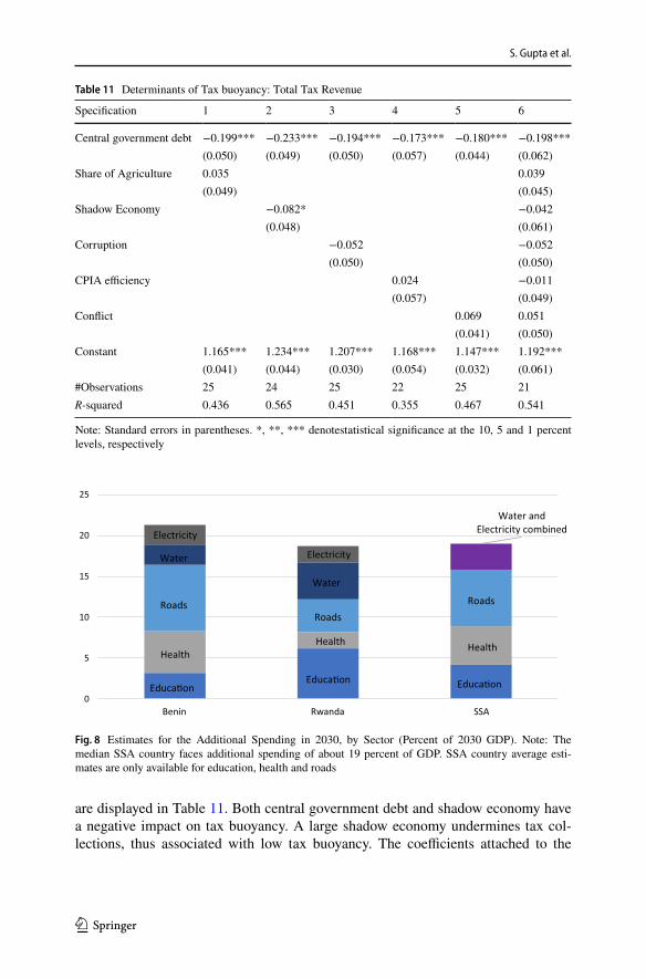
are displayed in Table 11. Both central government debt and shadow economy have a negative impact on tax buoyancy. A large shadow economy undermines tax col-lections, thus associated with low tax buoyancy. The coefficients attached to the
Table 11 Determinants of Tax buoyancy: Total Tax Revenue
Note: Standard errors in parentheses. *, **, *** denotestatistical significance at the 10, 5 and 1 percent levels, respectively
Specification 1 2 3 4 5 6
Central government debt −0.199*** −0.233*** −0.194*** −0.173*** −0.180*** −0.198***(0.050) (0.049) (0.050) (0.057) (0.044) (0.062)
Fig. 8 Estimates for the Additional Spending in 2030, by Sector (Percent of 2030 GDP). Note: The median SSA country faces additional spending of about 19 percent of GDP. SSA country average esti-mates are only available for education, health and roads
1 3
Tax Buoyancy in Sub-Saharan Africa and its Determinants
share of agriculture, corruption, efficiency of revenue mobilization and conflict are not statistically significant. Thus, the institutional quality as captured by corruption index and efficiency of revenue mobilization is not particularly relevant to reactions of taxes to GDP changes in SSA countries.
6 Estimation of additional revenue generated by 2030
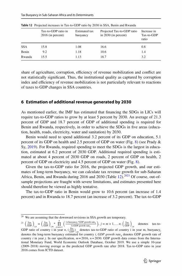
As mentioned earlier, the IMF has estimated that financing the SDGs in LICs will require tax-to-GDP ratios to grow by at least 5 percent by 2030. An average of 21.3 percent of GDP and 18.7 percent of GDP of additional spending is required for Benin and Rwanda, respectively, in order to achieve the SDGs in five areas (educa-tion, health, roads, electricity, water and sanitation) by 2030.
Benin would need to spend additional 3.2 percent of its GDP on education, 5.1 percent of its GDP on health and 2.5 percent of GDP on water (Fig. 8) (see Prady & Sy, 2019). For Rwanda, required spending to meet the SDGs is the largest in educa-tion, estimated at 6.2 percent of 2030 GDP. Additional required spending is esti-mated at about 4 percent of 2030 GDP on roads, 2 percent of GDP on health, 2 percent of GDP on electricity and 4.5 percent of GDP on water (Fig. 8).
Given the tax-to-GDP ratio for 2016, the projected GDP growth, and our esti-mates of long-term buoyancy, we can calculate tax revenue growth for sub-Saharan Africa, Benin, and Rwanda during 2016 and 2030 (Table 12).2021 Of course, out-of-sample projections are fraught with severe limitations, and estimates presented here should therefore be viewed as highly tentative.
The tax-to-GDP ratio in Benin would grow to 10.6 percent (an increase of 1.4 percent) and in Rwanda to 18.7 percent (an increase of 3.2 percent). The tax-to-GDP
Table 12 Projected increases in Tax-to-GDP ratio by 2030 in SSA, Benin and Rwanda
20 We are assuming that the downward revisions in SSA growth are temporary.21
�
Tax
GDP
�
i,n=
�
Tax
GDP
�
i,m*
n∏
j=m+1
�
1+buoyancyi*GDP growth rateij
1+GDP growth rateij
�
, j = m + 1,… n;�
Tax
GDP
�
i,n denotes tax-to-
GDP ratio of country i in year n, ( Tax
GDP)i,m
denotes tax-to-GDP ratio of country i in year m, buoyancyi denotes the long-term buoyancy estimated for country i, GDP growth rateij denotes GDP growth rate of country i in year j. In our specification, m = 2016, n = 2030. GDP growth data comes from the Interna-tional Monetary Fund, World Economic Outlook Database, October 2019. We use a simple 10-year (2009–2018) moving average as the predicted GDP growth rate after 2018. Tax-to-GDP ratio in year 2016 comes from ICTD dataset.
S. Gupta et al.
1 3
ratio for SSA as a region would grow modestly by 0.8 percent. In all cases, incre-mental taxes generated by 2030 would fall short of the average 5 percent of GDP additional revenues needed by LICs to finance the SDGs, and the shortfall would be large for two countries (Rwanda and Benin) for which detailed resource estimates exist. This suggests that it is imperative that countries in sub-Saharan Africa con-tinue to implement tax reforms to make their systems more responsive to income changes. At the same time, policymakers in Africa must complement tax-enhancing efforts with those directed at improving the quality of spending. It is possible to gen-erate up to 3 percent of GDP in resources by focusing on improving the efficiency of existing budget allocations (Gupta, 2018).
7 Concluding remarks and future research
In this paper, we estimated the short- and long-term tax buoyancies of 44 SSA countries between 1980 and 2017 using both time series and panel data techniques. Short-term buoyancy of PIT is significantly less than one. This could be attributable to wage rigidity in the formal sector. The estimated long-term buoyancy suggests that most taxes are progressive, except for those on trade. Overall, the robustness checks show that tax buoyancy is neutral to discretionary tax changes. The good news is that there is an increase in long-term buoyancy in the more recent period in reflection of tax reforms implemented by SSA countries. The future tax reforms would need to capture the changing economic structure to improve buoyancy. The cross-country determinants of long-term tax buoyancy suggest that both central government debt and shadow economy exert downward pressure on tax buoyancy. Our estimates suggest that domestic tax revenues generated by 2030 would not be adequate to cover spending needed to achieve the SDGs in SSA and two countries, Benin and Rwanda. The revenue shortfall could be larger if the spread of COVID-19 were to dampen SSA’s growth prospects over a long period. It could also delay implementation of critical tax reforms as countries seek to mitigate the virus’ impact through a fiscal stimulus.
Future research could study how tax buoyancy is affected by tax reforms by esti-mating time-varying long-term tax buoyancies in SSA countries and then assessing their determinants, including discretionary tax reforms.
Appendix
See Tables 13, 14, 15 and 16.
1 3
Tax Buoyancy in Sub-Saharan Africa and its Determinants
Tabl
e 13
Pr
ojec
ted
Incr
ease
s in
Tax-
to-G
DP
ratio
by
2030
in S
SA, B
enin
and
Rw
anda
Tax
buoy
anci
es a
re n
ot se
nsiti
ve to
lag
leng
th in
the
case
of t
otal
tax
reve
nue.
For
tax
com
pone
nts,
resu
lts v
ary
a PMG
esti
mat
or is
not
feas
ible
Tota
l tax
reve
nue
CIT
PIT
TGS
Trad
e ta
xes
p =
q =
2p
= q
= 1
p =
q =
2p
= q
= 1
p =
q =
2p
= q
= 1
p =
q =
2p
= q
= 1
p =
q =
2p
= q
= 1
Long
term
buo
yanc
y1.
158*
**1.
087*
**0.
877*
**1.
235*
**1.
204*
**1.
304*
**1.
353*
**1.
241*
**0.
832*
**0.
655*
**(0
.039
)(0
.048
)(0
.280
)(0
.011
)(0
.109
)(0
.177
)(0
.145
)(0
.077
)(0
.119
)(0
.136
)Sh
ort t
erm
buo
yanc
y0.
936*
**0.
960*
**10
.61.
40.
341*
0.64
1***
1.20
7***
1.12
4***
1078
***
1.21
3(0
.095
)(0
.094
)(0
.254
)(0
.206
)(0
.181
)(0
.142
)(0
.300
)(0
.266
)(0
.182
)(0
.183
)Sp
eed
of A
djus
tmen
t−
0.44
0***
−0.
410*
**-0
.775
***
-0.5
19−
0.55
5***
−0.
459*
**-0
.493
***
-0.4
53**
*-0
.431
-0.4
59(0
.040
)(0
.032
)(0
.087
)(0
.055
)(0
.084
)(0
.038
)(0
.069
)(0
.050
)((
0.04
5)(0
.038
)Es
timat
orM
GM
GM
GPM
Ga
MG
MG
MG
MG
MG
MG
S. Gupta et al.
1 3
Tabl
e 14
Pa
nel u
nit r
oot t
est i
n le
vels
Fish
er-ty
pe te
sts (c
ombi
ning
p-v
alue
s)
GD
PTa
x re
venu
eC
ITPI
TTG
STr
ade
Stat
istic
P-Va
lue
Stat
istic
P-Va
lue
Stat
istic
P-Va
lue
Stat
istic
P-Va
lue
Stat
istic
P-Va
lue
PIT
P-Va
lue
Inve
rse
chi-s
quar
ed (8
0) P
110.
010.
0165
.30.
8872
.72
0.52
70.8
00.
7597
.05
0.09
71.5
50.
738
Z1.
480.
933.
400.
992.
890.
993.
060.
991.
220.
882.
220.
98In
vers
e lo
git t
(204
) L*
1.39
0.91
3.74
0.99
2.64
0.99
2.94
0.99
1.00
0.84
2.01
0.97
Mod
ified
inv.
chi
-squ
ared
Pm
2.37
0.00
–0.
87–
0.54
–0.
761.
340.
08–
0.74
1.15
0.10
0.72
0.66
1 3
Tax Buoyancy in Sub-Saharan Africa and its Determinants
Tabl
e 15
Pa
nel u
nit r
oot t
est i
n fir
st di
ffere
nces
Usi
ng th
e K
ao te
st, w
e re
ject
the
null
hypo
thes
is o
f no
coin
tegr
atio
n at
1%
, 5%
and
10%
sign
ifica
nce
leve
ls
Fish
er-ty
pe te
sts (c
ombi
ning
p-v
alue
s)
GD
PTa
x re
venu
eC
ITPI
TTG
STr
ade
Stat
istic
P-Va
lue
Stat
istic
P-Va
lue
Stat
istic
P-Va
lue
Stat
istic
P-Va
lue
Stat
istic
P-Va
lue
PIT
P-Va
lue
Inve
rse
chi-s
quar
ed (8
0) P
251.
620
303.
970
311.
220
212.
830
238.
110
375.
930
Z–
0–
––
––
1.48
11.1
10
11.2
50
6.83
08.
920
12.6
30
––
––
––
Inve
rse
logi
t t(2
04) L
*9.
990
12.6
30
14.2
07.
850
9.77
015
.94
0M
odifi
ed in
v. c
hi-s
quar
ed P
m13
.56
017
.70
019
.50
010
.50
012
.49
023
.39
0
S. Gupta et al.
1 3
Tabl
e 16
C
oint
egra
tion
test
of G
DP
and
tax
reve
nues
Kao
(199
9) te
st fo
r coi
nteg
ratio
n
Tax
reve
nue
CIT
PIT
TGS
Trad
e ta
xes
Stat
istic
P-Va
lue
Stat
istic
P-Va
lue
Stat
istic
P-Va
lue
Stat
istic
P-Va
lue
Stat
istic
P-Va
lue
Mod
ified
Dic
key-
Fulle
r t−
3.82
30.
0001
–0.
0022
–0.
0057
–0.
0004
1.30
720.
0956
–2.
8475
2.52
873.
3238
Dic
key-
Fulle
r t4.
1235
04.
8875
0−
3.42
6–
1.08
03–
0.00
14–
0.00
02–
0.09
535.
7813
01.
8619
Aug
men
ted
Dic
key-
Fulle
r t2.
9933
3.54
830
11.2
5−
5.39
90
0U
nadj
uste
d m
odifi
ed D
icke
y-Fu
ller t
–0
––
0.00
06–
0–
0.18
276.
7612
8.51
650
3.21
836.
1853
0.90
62–
0–
–0.
0001
–U
nadj
uste
d D
icke
y-Fu
ller t
5.40
827.
5058
03.
7727
7.06
080
0.68
340.
2472
Num
ber o
f pan
els
4037
4040
40A
vg. n
umbe
r of p
erio
ds33
.119
.919
.326
26.9
1 3
Tax Buoyancy in Sub-Saharan Africa and its Determinants
Acknowledgements We would like to thank two anonymous referees as well as Masood Ahmed, Michael Clemens, and Mark Plant for valuable suggestions on an earlier version of the paper. We are grateful to the Bill & Melinda Gates Foundation for financial support. The usual disclaimer applies, and any remain-ing errors are the authors´ own responsibility.
References
Ahmad, E., & Stern, N. (1991). The theory and practice of tax reform in developing countries. Cam-bridge University Press.
Akitoby, B., Baum, A., Hackney, C., Harrison, O., Primus, K., Salins, V. (2019). Tax revenue mobiliza-tion episodes in developing countries. Policy Design and Practice, 3(1).
Bayu, T. (2015). Analysis of tax buoyancy and its determinants in Ethiopia (Cointegration Approach). Journal of Economics and Sustainable Development, 6(3), 182–194.
Bekoe, W., Danquah, M., & Senahey, S. K. (2016). Tax reforms and revenue mobilization in Ghana. Journal of Economic Studies, 43(4), 522–534.
Belinga, V., Benedek, M.D., De Mooij, R.A. & Norregaard, M.J. (2014). Tax buoyancy in OECD coun-tries. IMF Working Paper WP/14/110, Washington.
Benedek, D., Crivelli, E., Gupta, S., & Muthoora, P. (2014). Foreign aid and revenue: Still a crowding-out effect?. FinanzArchiv/Public Finance Analysis, pp 67–96.
Brückner, M. (2012). An instrumental variables approach to estimating tax revenue elasticities: Evidence from Sub-Saharan Africa. Journal of Development Economics, 98(2), 220–227.
Clements, B., Gupta, S., & Inchauste, G. (2004). Helping countries develop: the role of fiscal policy. International Monetary Fund.
Crivelli, E., & Gupta, S. (2014). Resource blessing, revenue curse? Domestic revenue effort in resource-rich countries. European Journal of Political Economy, 35, 88–101.
Deli, Y., Rodriguez, A.G., Kostarakos, I., & Varthalitis, P. (2018). Dynamic tax revenue buoyancy esti-mates for a panel of OECD countries. ESRI Working Paper, No. 592. Dublin, Ireland: The Eco-nomic and Social Research Institute.
Dudine, P., & Jalles, J. T. (2018). How buoyant is the tax system? New evidence from a large heterogene-ous panel. Journal of International Development, 30(6), 961–991.
Furceri, D., & Jalles, J. T. (2016). Determinants and effects of fiscal stabilization: New evidence from time-varying estimates. IMF Working Paper forthcoming.
Gaspar, V., Jaramillo, L., & Wingender, M.P. (2016). Tax capacity and growth: Is there a Tipping point? International Monetary Fund.
Gaspar, V., Amaglobeli, M.D., Garcia-Escribano, M.M., Prady, D., & Soto, M. (2019). Fiscal policy and development: human, social, and physical investments for the SDGs. International Monetary Fund.
Gillis, M. (2001). Experience with the VAT. Policy Science, 34(2), 195–215.Granger, C. W. J., & Terasvirta, T. (1993). Modelling Nonlinear Economic Relationships. Oxford Univer-
sity Press.Gupta, S. & Plant, M. (2019). Enhancing Domestic Resource Mobilization: What are the Real Obsta-
cles?” April 30, 2019. https:// www. cgdev. org/ blog/ enhan cing- domes tic- resou rce- mobil izati on- what- are- real- obsta cles.
Gupta, S. (2018). Merely collecting more taxes is not enough to achieve the SDGs, July 17, 2018. https:// www. cgdev. org/ blog/ merely- colle cting- more- taxes- not- enough- achie ve- sdgs.
Jalles, J. T. (2017). Tax Buoyancy in Sub-Saharan Africa: An empirical exploration. African Develop-ment Review, 29(1), 1–15.
Kao, C. (1999). Spurious regression and residual-based tests for cointegration in panel data. Journal of Econometrics, 90(1), 1–44.
Kargbo, B. I. B., & Egwaikhide, F. O. (2012). Tax elasticity in Sierra Leone: A time series approach. International Journal of Economics and Financial Issues, 2(4), 432–447.
Kusi, N.K. (1998). Tax reform and revenue productivity in Ghana. African Economic Research Consor-tium Research Paper No. 74, Nairobi
Lagravinese, R., Liberati, P., Sacchi, A. (2020). Tax buoyancy in OECD countries: new empirical evi-dence, Journal of Macroeconomics, 63.
McNabb, K. (2018). Tax Structures and economic growth: New evidence from the government revenue dataset. Journal of International Development, 30(2), 173–205.
Medina, L., Jonelis, A.W., & Cangul, M. (2017). The Informal Economy in Sub-Saharan Africa: Size and Determinants. IMF Working Paper WP/17/156, Washington.
Mullins, P., Gupta, S., & Liu, J. (2020), Domestic Revenue Mobilization in Low Income Countries: Where To From Here?. Center for Global Development Policy Paper 195, Washington
Osoro NE. (1993). Revenue productivity implications of tax reform in Tanzania. African Economic Research Consortium Research Paper No. 20, Nairobi
Pesaran, M. H., & Smith, R. P. (1995). Estimating long-run relationships from dynamic heterogeneous panels. Journal of Econometrics, 68, 79–113.
Pesaran, M. H., Shin, Y., & Smith, R. P. (1999). Pooled mean group estimation of dynamic heterogeneous panels. Journal of the American Statistical Association, 94(446), 621–634.
Prady, D., & Sy, M. (2019). The spending challenge for reaching the SDGs in Sub-Saharan Africa: Les-sons learned from Benin and Rwanda. IMF Working Paper WP/19/270, Washington.
Shikongo, A., Kakujaha-Matundu, O., & Kaulihowa, T. (2019). Revenue productivity of the Tax System in Namibia: Tax buoyancy estimation approach. Journal of Economics and Behavioral Studies, 11(2 (J)), 112–119.
Stotsky JG, & Wolde-Mariam A. (1997). Tax effort in sub-Saharan Africa. IMF Working Paper WP/97/107, Washington.
Tanzi, V., & Zee, H. (2000). Tax policy for emerging markets: Developing countries. IMF Working Paper WP/00/35, Washington.
Teera, J. M., & Hudson, J. (2004). Tax performance: A comparative study. Journal of International Development, 16(6), 785–802.
Publisher’s Note Springer Nature remains neutral with regard to jurisdictional claims in published maps and institutional affiliations.