Page 1
1
Tax changes and economic growth:
Empirical evidence for a panel of OECD
countries*
Davide Furceri #
OECD and University of Palermo
Georgios Karras ##
University of Illinois at Chicago
Abstract
This paper investigates the effects of changes in taxes on economic growth. Using annual
data from 1965 to 2007 for a panel of twenty-six economies, the results show that the effect
of an increase in taxes on real GDP per capita is negative and persistent: an increase in the
total tax rate (measures as the total tax ratio to GDP) by 1% of GDP has a long-run effect on
real GDP per capita of –0.5% to –1%. Our findings also imply that an increase in social
security contributions or taxes on goods and services has a larger negative effect on per
capita output than an increase in the income tax.
JEL classification: E62, H30
Keywords: Taxes, Economic Growth
* We would like to thank Ad van Riet for useful comments. The opinions expressed herein are those of the
authors and do not necessarily reflect those of the OECD and its members countries.
# Mailing Address: OECD, 2 rue Andre Pascal, 75775 Paris Cedex 16. Email: [email protected] ,
[email protected] . ## Corresponding author. Mailing address: University of Illinois at Chicago, Department of Economics, 601
South Morgan Street, 60607 Chicago, IL. E-mail: [email protected] .
Page 2
2
1. Introduction
The effect of taxes on aggregate economic activity is one of the least contested areas
in theoretical macroeconomics. Both neoclassical and Keynesian theoretical models, for
example, predict that higher taxes reduce economic activity, even though there is less
agreement on the exact mechanisms that generate this result.1
However, in spite of this, albeit imperfect, consensus (or perhaps because of it), the
issue has not been pursued empirically with anything like the dedication that has
characterized the much more vigorously debated effects of monetary policy. The most recent
important exception has been the study by Romer and Romer (2007) who construct a novel
measure of “exogenous” tax shocks and estimate its short-run and long-run economic
effects.2
The goal of the present paper is to contribute to the empirical side of the question
using a panel methodology that analyzes annual data from the 1965 to 2003 period for 26
OECD economies. Our empirical findings show that higher taxes do indeed result in a
reduction of GDP per capita that is sizable and persistent. While the exact size of the effect
depends on how the “tax shock” is measured, our estimates suggest that an increase in the
total tax rate by 1% of GDP will have a long-run effect on GDP per capita of –0.5% to –1%.
This is smaller than Romer and Romer’s (2007) rather large estimated effect (approximately
1 See, for example, Eaton (1981), Dotsey (1990), King and Rebelo (1990), Rebelo (1991), Jones et al.
(1993, 1997), Stokey and Rebelo (1995), Milesi-Ferretti and Roubini (1998), Kims (1998).
2 Other recent examples of empirical studies include Reinhar and Kormendi (1989), Easterly and Perotti
(1993a), Easterly and Perotti (1993b), Agell et al. (1997, 1999, 2006), Bleaney et al. (2001), Folster and
Nerekson (1999, 2001, 2006) Perotti (1999), Karras (1999), Daveri and Tabellini (2000), Bleaney et al.
(2001), Folster and Nerekson (1999, 2001, 2006), Blanchard and Perotti (2002), Afonso and Furceri (2008)
Arnold (2008), Johansson et al. (2008).
Page 3
3
–3%), but much closer to the effects obtained by Karras (1999) for a smaller OECD sample,
and by Blanchard and Perotti (2002) for the U.S.
We also look at the effects of four of the largest types of taxes: taxes on income,
profits, and capital gains; taxes on property; social security contributions; and taxes on goods
and services. We find that they all have negative effects on GDP per capita (though not
statistically significant in the case of property taxes), and that an increase in social security
contributions or taxes on goods and services has a larger negative effect on per capita output
than an increase in the income tax.
The rest of the paper is organized as follows. Section 2 discusses the sources of the
data and defines the variables to be used in the estimation. Section 3 outlines the estimation
methodology, derives the main empirical results, and implements a number of robustness
checks. Section 4 discusses the findings and some possible extensions, and concludes.
2. The Data
The data cover 26 OECD countries and are obtained from OECD’s Statistical
Compendium on CD-ROM for the time period 1965-2007. All tax data are from the Revenue
Statistics of OECD Member Countries database, and measure various taxes as a percentage
of GDP. In addition to (i) the total tax rate, we also focus on (ii) taxes on income, profits,
and capital gains, (iii) social security contributions, (iv) taxes on property, and (v) taxes on
goods and services. Our other main variable of interest is growth, the growth rate of real
GDP per capita. Both real GDP and population data are obtained from the OECD’s
Economic Outlook database.
Page 4
4
Table 1 provides a list of these 26 OECD economies together with country averages
over 1965-2007 for the growth and the five tax series.3 Average annual growth of real GDP
per capita has ranged from 1.3% in Switzerland to 4.2% in Ireland. Over the same time
period, the average total tax to GDP ratio has varied from 17.6% in Mexico to 46.1% in
Sweden. Though these OECD countries have relied very differently on the various forms of
taxes, income taxation has been the largest revenue generator for most of them.4 Taxes on
income, profits, and capital gains have ranged from 4.76% of GDP in Mexico to 25.% of
GDP in Denmark. In nine of the countries, most revenue has been raised by taxes on goods
and services.5 Only in three countries has the largest share been generated by social security
taxes,6 and in none of the countries by property taxes, which are generally the smallest.
Figure 1 plots the cross-sectional relationship between the average growth rate of real
GDP per capita and the averaged total tax rate for the 26 countries of our sample over 1965-
2007. The relationship is moderately negative (the correlation coefficient between the two
variables is –0.32)7.
On the face of it, this negative correlation is consistent with the theoretically
predicted inverse relationship between taxation and economic growth. However, while it
3 Country selection is dictated by data availability only. Social security contributions were unavailable
for Australia and New Zealand.
4 To be specific, for 14 countries out of the 26: Australia, Belgium, Canada, Denmark, Finland, Japan,
Luxembourg, the Netherlands, Norway, New Zealand, Sweden, Switzerland, the UK, and the US.
5 The nine are Austria, Greece, Iceland, Ireland, Korea, Mexico, Portugal, Spain, and Turkey.
6 These three are France, Germany, and Italy.
7 Figure 1 suggests that Korea may be regarded as an outlier. Indeed, repeating the computation excluding
Korea from the sample, the correlation is -0.15.
Page 5
5
may be tempting to read it as evidence supportive of this theoretical proposition, we believe
it would be imprudent to interpret it as causal.
Figure 2 repeats the correlation exercise for the four categories of taxes mentioned
above, by looking at the cross-sectional relationship between average growth and each of
these four taxes over 1965-2007. As Figure 2 makes clear, the cross-sectional relationship is
negative between average growth and the average income tax rate (the correlation coefficient
is –0.42); also negative between average growth and the average social security tax rate
(correlation –0.28); weakly negative between average growth and the average property tax
rate (correlation -0.07); and weakly positive between average growth and the tax rate on
goods and services (correlation 0.08)8. Once again, we would caution against a causal
interpretation of these correlations.
Figures 3 and 4 add a time dimension to these numbers. Figure 3 shows how the total
tax rate has evolved in each of the 26 countries, while Figure 4 graphs the growth rates of
real GDP per capita for each of the 26 economies. The most striking feature of Figure 3 is
that the “long-term trend” in each of the 26 countries has been positive, in the sense that all
total tax rates in 2007 exceed those of 1965. The pattern for the tax rate, however, differs
substantially. Whereas many of the countries (such as Australia, Austria, Greece, Korea, and
Portugal) have been fluctuating around a mostly upward sloping path, others (such as
Germany, Mexico, the UK, and the US) have been much steadier, or have followed hump-
shaped patterns (like those of Ireland, Japan, and the Netherlands).
8 Also figure 2 suggests that Korea may be regarded as an outlier. Indeed, repeating the computations for
different types of taxes excluding Korea from the sample, the correlation are -0.34 for income tax, -0.12 for
social security tax, -0.12 for property tax, and 0.20 for tax on goods and services.
Page 6
6
This substantial variability both across countries and over time should facilitate the
empirical identification of the effects of tax changes on growth. We now turn to a model that
will attempt to do just that.
3. Evidence on the Effects of Taxes on Growth
3.1. The benchmark model
We start with the simplest possible dynamic approach that relates growth and the tax
rate, a model similar to the empirical specification in Romer and Romer (2007):
ti
J
j
jtijtiti udtaxbvwgrowth ,
0
,, +++= ∑=
−, (1)
where growth is the growth rate of real GDP per capita, i is indexing over countries and t
over time, w and v represent country- and time-specific effects, the b’s are parameters to be
estimated, dtax is the change in the tax rate ( 1,,, −−= tititi taxtaxdtax ), J is the number of lags,
and u is the error term.
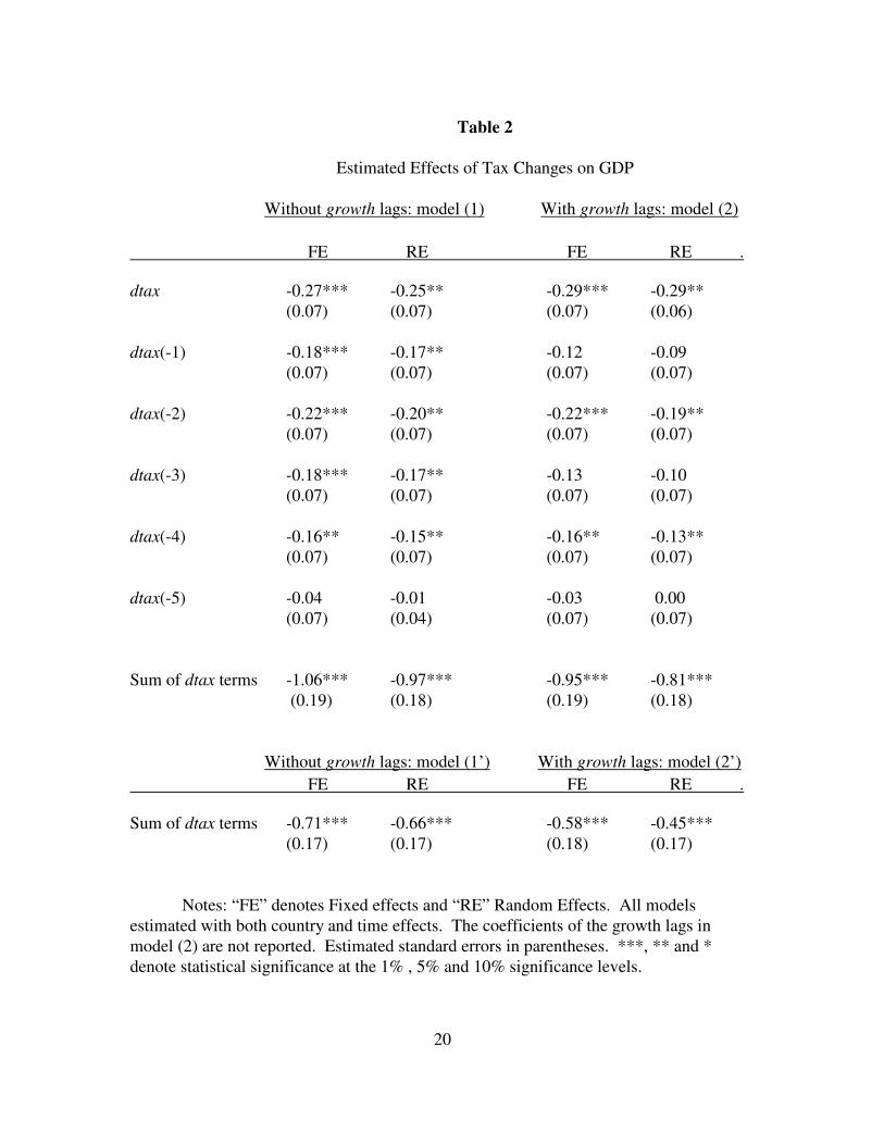
The first two columns of Table 2 estimate equation (1) for J = 5.9 The first column
models the w’s and v’s as fixed effects (FE), and the second column as random effects (RE).
Interestingly, all estimated b’s have a negative sign, and all but the 5th
lags are statistically
significant. In addition, the differences between the fixed-effects and random-effects
specifications are very small.
9 Different lag lengths were also tried, but the contemporaneous term and the first four lags are generally
statistically significant. The model was also estimated without country- or time-specific effects, and with
only country fixed or random effects. Results are very robust and are not reported to preserve space. All
results are available on request.
Page 7
7
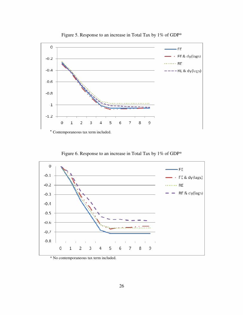
The “FE” and “RE” lines of Figure 5 plot the estimated response of real GDP to an
increase in the total tax rate by 1% of real GDP, using the estimated parameters of the first
two columns of Table 2. These “impulse response functions” show that such an increase in
the tax rate immediately reduces GDP. The decline then continues for about four to five
years, when the cumulative decrease in GDP has reached approximately 1%. This long-run
effect of the tax increase on GDP is captured by the sum of the estimated b coefficients. As
Table 2 shows, the sum of the estimated b’s is –1.06 for the fixed-effects specification, and –
0.97 for random effects. Both are negative and highly statistically significant. This suggests
that changes in the total tax rate have a statistically significant negative effect on GDP that is
both sizable and persistent.
The rest of this section investigates the robustness of this result. The most obvious
correction has to do with the presence of serial correlation.10
To allow for this, we modify
model (1) to:
ti
J
j
jtij
K
j
jtijtiti udtaxbgrowthavwgrowth ,
0
,
1
,, ++++= ∑∑=
−
=
−, (2)
where the a’s are parameters to be estimated.
The last two columns of Table 2 estimate equation (2) and report the estimated b’s for
J = K = 5 (the estimated a’s are not reported to preserve space). Once more, all estimated b’s
have a negative sign, and now the contemporaneous tax terms, as well as the 2nd
and 4th
lags,
are statistically significant. Again, the differences between the fixed-effects and random-
10
When we used ρ , the estimated AR(1) parameter for the residuals, as proposed by Wooldridge (2002),
serial correlation was detected in both the FE and RE specifications. Instead of imposing a first-order
structure, however, we prefer to allow for the more general form of model (2).
Page 8
8
effects specifications are virtually nil, and the sums of the estimated b’s are negative (–0.95
with fixed effects and –0.81 with random effects) and highly statistically significant.
The “FE & dy(lags)” and “RE & dy(lags)” lines of Figure 5 plot the estimated
response of GDP to an increase in the total tax rate by 1% of GDP, using the estimated
parameters of model (2). It is readily apparent that these are very close to those obtained
from model (1). It follows that allowing for autoregressive structure, does not alter our
conclusion that changes in the total tax rate have a statistically significant negative effect on
growth that is both sizable and persistent.11
3.2. Additional Robustness Extensions
Unlike Romer and Romer’s (2007) tax measure, ours is not guaranteed to be
exogenous. Our estimated b’s in models (1) and (2), therefore, could be biased. We address
this issue of potential bias in four different ways. First, we eliminate the contemporaneous
dtax term in models (1) and (2). Second, we correct for the effects of economic activity on
tax revenue, in the spirit of Perotti (1999), and Blanchard and Perotti (2002). Third, we
estimate the impact of taxes on growth by using the GMM approach proposed by Arellano
and Bover (1995) and Blundell and Bond (1998). Fourth, we consider 5 years moving
averages in order to iron out business cycle fluctuations.
For the first, more modest fix, we simply revise models (1) and (2) to:
ti
J
j
jtijtiti udtaxbvwgrowth ,
1
,, +++= ∑=
−, (1’)
11
This is similar to the finding of Romer and Romer (2007).
Page 9
9
and
ti
J
j
jtij
K
j
jtijtiti udtaxbgrowthavwgrowth ,
1
,
1
,, ++++= ∑∑=
−
=
−, (2’)
respectively, thereby simply excluding the contemporaneous tax term from the original
equations. We do not report the estimated a’s and b’s because of space considerations, but
we report the sums of the estimated b’s and we summarize the dynamic responses of an
increase in the tax rate.
The sums of the estimated b’s from models (1’) and (2’) are reported in the last row
of Table 2, for both the fixed-effects and random-effects specifications. It can be seen that
all four are negative and statistically significant, just like the sums of the estimated b’s from
models (1) and (2). However, they are smaller in absolute value than the sums from the
models that include the contemporaneous tax term, which is not surprising since the excluded
contemporaneous term is amply negative.
Figure 6 summarizes the estimated responses of GDP to an increase in the total tax
rate by 1% using models (1’) and (2’) with fixed and random effects. The pattern of these
responses is virtually identical to that of Figure 5, the only difference being the somewhat
smaller long-run effects.
The second robustness check considered in this subsection intends to construct a
more exogenous measure of changes in the tax rate. To that end, we estimate the VAR-type
system
ti
J
j
jtij
J
j
jtijtiti growthfdtaxczxdtax ,
1
,
1
,, τ++++= ∑∑=
−
=
−, (3)
Page 10
10
and
ti
J
j
jtij
K
j
jtijtiti ugrowthadtaxbvwgrowth ,
1
,
1
,, ++++= ∑∑=
−
=
−, (4)
where x and z (like w and v) represent country- and time-specific effects, and the c’s and f ’s
(like the a’s and b’s) are parameters to be estimated. Equation (4) is a special case of (2’).
Equation (3) allows dtax to respond to growth, recognizing the fact that economic activity
plays a role in the determination of the tax rate. We interpret τ as an “exogenous” tax rate
shock.
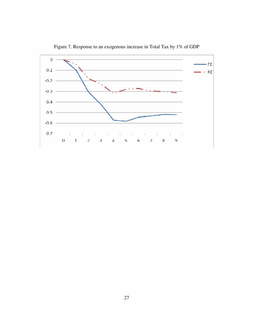
We estimate the system of equations (3) and (4), and plot in Figure 7 the estimated
dynamic responses of GDP to an exogenous tax-rate shock of 1% of GDP for the two
specifications of fixed (“FE”) and random (“RE”) effects for J = 5. While quantitatively
these effects are weaker (and more so for the random effects specification) than those of the
plain tax changes, the pattern of these impulse response functions is very similar to the plots
of Figures 5 and 6: a positive tax rate shock has a negative and persistent effect on GDP.
In order to control for endogeneity and provide robustness for our results, we also
estimate model (2) using the GMM approach proposed by Arellano and Bover (1995) and
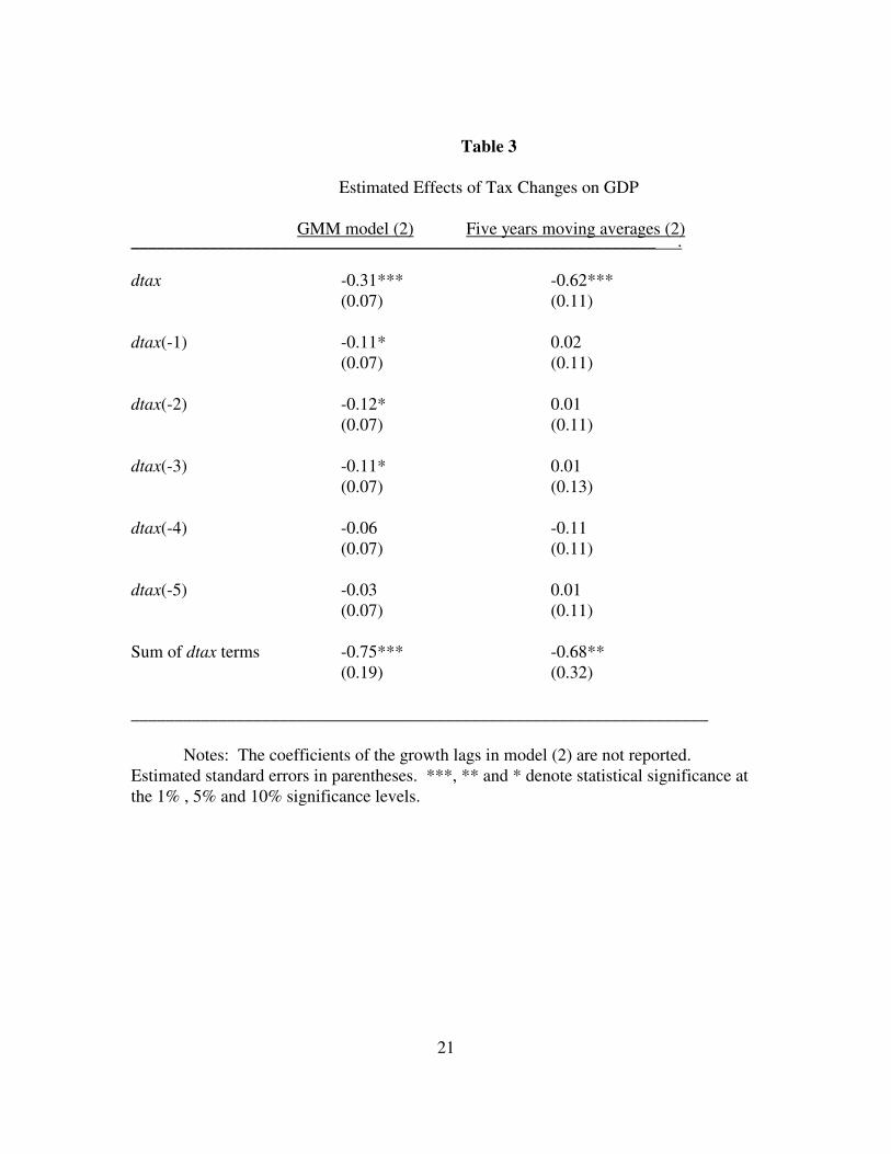
Blundell and Bond (1998). The results are reported in the first column of Table 3. Analyzing
the Table we can see that both the current values of dtax as well as its three lags are
statistically significant. Moreover, the sum of the estimated b’s is –0.75, which is negative
and highly statistically significant.
The fourth robustness check consists of estimating model (2) using years moving
averages in order to iron out cyclical fluctuations (Bleaney et al. 2001). The results are
Page 11
11
reported in the second column of Table 3. While, as it is possible to expect, the lag of dtax
are not statistically significant, the current value of dtax as well as the cumulative effect is
statistically significant and is magnitude is comparable to the one obtained using yearly data.
Finally is worth to mention that unlike the correlation charts presented in Figure 1
and 2, all the estimated results are robust to the inclusion of Korea in our sample.
3.3. The Effects of Different Types of Taxes
We now ask whether our four available types of taxes (income, property, social
security, and goods and services) have similar effects on per capita real GDP growth with
those we observed above for the total tax rate, and whether differences exist among them, as
often suggested by economic theory.
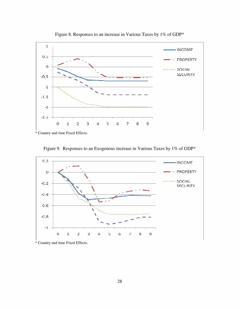
We begin by estimating the benchmark model (1) for each of the four types of tax,
and plot in Figure 8 the estimated responses of GDP to an increase in each of the four tax
types by 1% of GDP. An increase in income taxes, social security taxes, and taxes on goods
and services is followed by an immediate drop in GDP which continues for three to five
years, until it stabilizes at a lower level.
An increase in property taxes, is associated with a counterintuitive short-run increase
in GDP; this effect disappears after three years and is actually reversed in the longer term,
eventually reducing GDP. However, the sum of the estimated b’s for the property taxes (–
0.53, with a standard error of 1.01) is not statistically significant.
The other three types of tax, however, have more sizable and statistically significant
growth effects. Interestingly, an increase in the social security contributions is predicted to
Page 12
12
have the largest negative growth effects, both in the short- and long-run. The sum of the
estimated b’s for the social security tax is –1.98 (standard error 0.41), which is twice as high
as the corresponding value we estimated for total taxes, and highly statistically significant.
Higher taxes on goods and services have the second most detrimental growth effects, with a
sum of estimated b’s equal to –1.38 (standard error 0.44). This is both statistically significant
and somewhat larger than the effect of total taxes. Finally, and somewhat surprisingly, taxes
on income, profits, and capital gains, have a smaller effect than either social security taxes or
taxes on goods and services. Their effects, however, are consistently negative and
statistically significant, with a sum of estimated b’s equal to –0.70 (standard error 0.28).
We know from the previous subsection that model (1) may overestimate the growth
effects of a tax change. Therefore, all other models discussed above for the total tax have
also been estimated for each of the four specific tax types. To preserve space, we only report
the results of estimating the VAR-type systems of equations (3) and (4). Figure 9 plots the
estimated dynamic responses of GDP to an “exogenous” tax-rate shock of 1% of GDP in
each of the four tax types. As expected, the responses of GDP to those exogenous tax shocks
are smaller in absolute value (roughly by one half) than the corresponding responses to raw
tax changes. The general picture, however, is unaffected. With the exception of the property
tax (whose short-term and long-term effects are statistically insignificant, just like before), an
increase in any of the other three types of tax has a negative and persistent effect on GDP.
Page 13
13
4. Discussion and Conclusions
This paper estimated the effects of tax changes on real GDP growth per capita using
annual data from the 1965 to 2003 period for a panel of 26 OECD economies.
The empirical findings show that an increase in taxes has a negative and persistent
effect on real GDP per capita. The size of the effect depends on how the “tax shock” is
measured, but our estimates suggest that an increase in the total tax rate by 1% of GDP will
have a long-run effect on real GDP per capita of –0.5% to –1%. This is smaller than Romer
and Romer’s (2007) rather large estimated effect (approximately –3%), but their
identification of a “tax shock” is very different from ours, and their measure of GDP is
aggregate (not per capita). In addition, our estimates are much closer to those of Karras
(1999) for a smaller OECD sample, and Blanchard and Perotti (2002) for the U.S.
We also look at the effects of what are usually the four largest types of taxes: taxes on
income, profits, and capital gains; taxes on property; social security contributions; and taxes
on goods and services. Our findings imply that all four have negative effects on real GDP
per capita, though those of property taxes are not statistically significant. Of the other three,
our estimates suggest that an increase in social security taxes or taxes on goods and services
has a larger effect on output than an increase in the income tax.
Our study suggests that a number of interesting extensions can be pursued. First, it
would be useful to examine the effects of taxes on variables other than income, such as
consumption, investment, employment, or unemployment.12
Preliminary evidence on
consumption and investment is presented in Figures 10 for the benchmark model (1) and
12
Daveri and Tabellini (2000), among others, have looked at the relationship between taxation and
Page 14
14
Figure 11 for the VAR-type system of equations (3) and (4). In each case, the original
variable growth (the growth rate of per capita GDP) has been replaced by the growth rate of
aggregate GDP, consumption, and investment (all in real terms, obtained form the OECD’s
Economic Outlook database).
Just like for the GDP per capita series, the evidence of Figures 10 and 11 shows that a
tax increase has a clear negative effect on aggregate GDP, consumption, and investment.
However, the effect of a tax change on investment is much larger than the effect on GDP or
consumption. This finding is robust to the construction of the tax “shocks” and the method
of estimation, and it is consistent with the findings of Blanchard and Perotti (2002) and
Romer and Romer (2007) who also estimated larger negative effects on investment than on
output or consumption.
Pursuing this further would be interesting not only because of the obvious importance
of these variables and others, but also because it can shed light on the way the effects of tax
changes are transmitted to the rest of the economy. It might also be worthwhile to include
government spending in the estimated models in order to capture possible interactions
between it and taxes.
An additional promising direction would be to investigate whether the effects of taxes
are asymmetric. One type of asymmetry includes effects that may be different (in absolute
value) for tax increases than tax decreases, as has been claimed for monetary policy.13
unemployment and growth.
13 In a long literature beginning with Cover (1992).
Page 15
15
Another type of asymmetry would test whether tax changes have different effects when
undertaken in different economic circumstances, as in Perotti (1999).
Page 16
16
References
Arelllano, M. and Bover, O. (1995), "Another look at the instrumental variables estimation of
error-component models", Journal of Econometrics, 68.
Arnold, J. (2008), “Do Tax Structures Affect Aggregate economic Growth? Empirical
Evidence forma a Panel of OECD Countries”, OECD Economics Department Working
Papers 643.
Afonso, A. and D. Furceri (2008), “Government size, composition, volatility and economic
growth," ECB Working Paper Series 849.
Agell, J., T. Lindh and H. Ohlsson (1997), “Growth and the Public Sector: A Critical Review
Essay”, European Journal of Political Economy 13: 33-52.
Agell, J., T. Lindh and H. Ohlsson (1999), “Growth and the Public Sector: A Reply”,
European Journal of Political Economy 15: 359-366.
Agell, J., H. Ohlsson and P.S. Thoursie (2006), “Growth Effects of Government Expenditure
and Taxation in Rich Countries: A Comment”, European Economic Review 50: 211-218.
Blanchard, O.J. and R. Perotti (2002), “An Empirical Characterization of the Dynamic
Effects of Changes in Government Spending and Taxes on Output”, Quarterly Journal of
Economics 117: 1329-1368.
Bleaney, M., N. Gemmell and R. Kneller (1999), “Fiscal Policy and Growth: Evidence from
OECD Countries”, Journal of Public Economics 74: 171-190.
Bleaney, M., N. Gemmell and R. Kneller (2001), “Testing the Endogenous Growth Model:
Public Expenditure, Taxation, and Growth over the Long Run”, Canadian Journal of
Economics 34: 36-57.
Blundell, R. and Bond, S. (1998), "Initial conditions and moment restrictions in Dynamic
Panel Data Models", Journal of Econometrics, 87.
Fölster, S. and M. Henrekson (1999), “Growth and the Public Sector: A Critique of the
Critiques”, European Journal of Political Economy 15: 337-358.
Fölster, S. and M. Henrekson (2001), “Growth Effects of Government Expenditure and
Taxation in Rich Countries”, European Economic Review 45: 1501-1520.
Fölster, S. and M. Henrekson (2006), “Growth Effects of Government Expenditure and
Taxation in Rich Countries: A Reply”, European Economic Review 50: 219-221.
Cover J.P., 1992. Asymmetric Effects of Positive and Negative Money-Supply Shocks.
Quarterly Journal of Economics 1992; 107; 1261-1282.
Daveri F, Tabellini G., 2000. Unemployment, Growth and Taxation in Industrial Countries.
Economic Policy 2000; April; 48-104.
Page 17
17
Dotsey M., 1990. The economic effects of production taxes in a stochastic growth model.
American Economic Review 1990; 80; 1168–1182.
Eaton J., 1981. Fiscal policy, inflation and the accumulation of risky capital. Review of
Economic Studies 1981; 48; 435–445.
Easterly W, Rebelo S., 1993a. Marginal income tax rates and economic growth in developing
countires. European Economic Review 1993a; 37; 409-417.
Easterly W, Rebelo S., 1993b. Fiscal policy and economic growth: An empirical
investigation. Journal of Monetary Economics 1993b; 32; 417-458.
Fölster, S. and M. Henrekson (1999), “Growth and the Public Sector: A Critique of the
Critiques”, European Journal of Political Economy 15: 337-358.
Fölster, S. and M. Henrekson (2001), “Growth Effects of Government Expenditure and
Taxation in Rich Countries”, European Economic Review 45: 1501-1520.
Fölster, S. and M. Henrekson (2006), “Growth Effects of Government Expenditure and
Taxation in Rich Countries: A Reply”, European Economic Review 50: 219-221.
Johansson, A., Heady, C., Arnold, J., Brys, B. and L. Vartia, (2008). "Taxation and
Economic Growth," OECD Economics Department Working Papers 620.
Jones L.E., Manuelli R.E., Rossi P.E., 1993 Optimal taxation in model of endogenous
growth. Journal of Political Economy 1993; 101; 485-517.
Jones L.E., Manuelli R.E., Rossi P.E, 1993. On the optimal taxation of capital income.
Journal of Economic Theory 1993; 73; 93-117.
Karras G., 1999. Taxes and Growth: Testing the Neoclassical and Endogenous Growth
Models Contemporary Economic Policy 1999; 17; 177-188.
Kims S.J., 1998. Growth effect of taxes in an endogenous growth model: to what extent do
taxes affect economic growth? - a puzzle. Journal of Economic Dynamics and Control 1998;
23; 125-158.
King R.G, Rebelo S.,1990. Public policy and economic growth: developing neo-classical
implications. Journal of Political Economy 1990; 98; 126-150.
Milesi-Fereti G.M., Roubini, N., 1998. Growth effects of income and consumption taxes.
Journal of Money, Credit and Banking 1998; 30; 721-744.
Perotti R., 1999. Fiscal Policy in Good Times and Bad. Quarterly Journal of Economics
1999; 114; 1399-1436.
Page 18
18
Rebelo S., 1991.Long-run policy analysis and long-run growth. Journal of Political Economy
1991; 99; 500-521.
Romer C. D., Romer, D.H, 2007. The Macroeconomic Effects of Tax Changes: Estimates
based on a new measure of Fiscal Shocks” NBER working paper 2007; 13264.
Stokey N., Rebelo S., 1995., Growth effects of flat-rate tax. Journal of Political Economy
1995; 103; 419-450.
Wooldridge, J.M., 2002. Econometric Analysis of Cross-Section and Panel Data. MIT Press,
Cambridge, Massachusetts, 2002.
Page 19
19
Table 1
Country Averages over 1965-2007
Taxes as a % of GDP .
Country growth total income property goods social security
1. Australia 2.1 26.7 14.9 2.5 8.0 NA
2. Austria 2.6 39.4 10.6 1.0 12.5 12.3
3. Belgium 2.4 41.3 15.4 1.5 11.5 12.8
4. Canada 2.1 32.8 15.0 3.4 9.7 4.0
5. Denmark 2.1 44.0 25.4 2.1 15.4 1.0
6. Finland 2.9 39.8 16.0 1.0 13.4 8.9
7. France 2.3 40.2 7.4 2.4 12.0 16.0
8. Germany 1.3 35.3 11.4 1.2 9.9 12.6
9. Greece 3.0 25.4 4.8 1.6 10.8 8.1
10. Iceland 2.7 32.6 10.7 2.3 16.6 2.0
11. Ireland 4.2 31.2 11.0 2.2 13.6 4.1
12. Italy 2.4 34.2 10.6 1.5 9.8 11.5
13. Japan 3.3 24.9 10.5 2.4 4.5 7.5
14. Korea 5.8 19.1 5.5 2.2 9.1 1.8
15. Luxembourg 3.2 34.6 13.7 2.5 8.5 9.6
16. Mexico 2.4 17.6 4.7 0.3 9.7 2.6
17. Netherlands 2.3 40.3 12.2 1.5 10.9 15.4
18. Norway 2.9 40.3 15.8 1.0 14.6 8.8
19. New Zealand 1.5 31.9 20.1 2.3 9.5 NA
20. Portugal 3.3 26.1 6.3 0.7 11.2 7.5
21. Spain 2.8 26.6 7.2 1.6 7.6 10.2
22. Sweden 2.1 46.1 20.0 1.1 12.1 11.3
23. Switzerland 1.3 25.3 11.3 2.2 5.9 5.8
24. Turkey 2.7 15.8 5.3 0.7 6.2 2.4
25. UK 2.2 35.2 13.6 4.2 10.8 6.0
26. USA 2.1 26.7 12.6 3.2 4.9 5.9
Notes: growth: the average annual growth rate of real GDP per capita.
All taxes are expressed as a percentage of GDP.
total: total taxes;
income: taxes in income, profits and capital gains;
property: taxes on property;
goods: taxes on goods and services; and
social security: social security taxes.
Page 20
20
Table 2
Estimated Effects of Tax Changes on GDP
Without growth lags: model (1) With growth lags: model (2)
FE RE FE RE .
dtax -0.27*** -0.25** -0.29*** -0.29**
(0.07) (0.07) (0.07) (0.06)
dtax(-1) -0.18*** -0.17** -0.12 -0.09
(0.07) (0.07) (0.07) (0.07)
dtax(-2) -0.22*** -0.20** -0.22*** -0.19**
(0.07) (0.07) (0.07) (0.07)
dtax(-3) -0.18*** -0.17** -0.13 -0.10
(0.07) (0.07) (0.07) (0.07)
dtax(-4) -0.16** -0.15** -0.16** -0.13**
(0.07) (0.07) (0.07) (0.07)
dtax(-5) -0.04 -0.01 -0.03 0.00
(0.07) (0.04) (0.07) (0.07)
Sum of dtax terms -1.06*** -0.97*** -0.95*** -0.81***
(0.19) (0.18) (0.19) (0.18)
Without growth lags: model (1’) With growth lags: model (2’) FE RE FE RE .
Sum of dtax terms -0.71*** -0.66*** -0.58*** -0.45***
(0.17) (0.17) (0.18) (0.17)
Notes: “FE” denotes Fixed effects and “RE” Random Effects. All models
estimated with both country and time effects. The coefficients of the growth lags in
model (2) are not reported. Estimated standard errors in parentheses. ***, ** and *
denote statistical significance at the 1% , 5% and 10% significance levels.
Page 21
21
Table 3
Estimated Effects of Tax Changes on GDP
GMM model (2) Five years moving averages (2) ____________________________________________________________ .
dtax -0.31*** -0.62***
(0.07) (0.11)
dtax(-1) -0.11* 0.02
(0.07) (0.11)
dtax(-2) -0.12* 0.01
(0.07) (0.11)
dtax(-3) -0.11* 0.01
(0.07) (0.13)
dtax(-4) -0.06 -0.11
(0.07) (0.11)
dtax(-5) -0.03 0.01
(0.07) (0.11)
Sum of dtax terms -0.75*** -0.68**
(0.19) (0.32)
__________________________________________________________________
Notes: The coefficients of the growth lags in model (2) are not reported.
Estimated standard errors in parentheses. ***, ** and * denote statistical significance at
the 1% , 5% and 10% significance levels.
Page 22
22
Figure 1. Growth of Real GDP per Capita vs Total Tax Rate, 1965-2007
AUS
AUTBEL
CAN DNK
FIN
FRA
DEU
GRE
ICE
IRE
ITA
JPN
KOR
LUX
MEXNLD
NZL
NOR
PRT
ESP
SWE
CHE
TUR
UKUSA
12
34
56
Gro
wth
of R
ea
l G
DP
per
Ca
pita
(p
erc
enta
ge p
oin
ts)
10 20 30 40 50Total Tax as % of GDP
Page 23
23
Figure2. Growth of Real GDP per Capita vs Various Tax Rates, 1965-2007
AUSAUTBEL
CAN DNK
FIN
FRA
DEU
GREICE
IRE
ITA
JPN
KOR
LUX
MEXNLD
NZL
NORPRT
ESP
SWE
CHE
TURUKUSA AUS
AUT BELCAN DNK
FIN
FRA
DEU
GREICE
IRE
ITA
JPN
KOR
LUX
MEX NLD
NZL
NORPRT
ESP
SWE
CHE
TURUKUSA
AUSAUT BEL
CANDNK
FIN
FRA
DEU
GREICE
IRE
ITA
JPN
KOR
LUX
MEX NLD
NZL
NORPRT
ESP
SWE
CHE
TURUKUSA
AUTBELCANDNK
FIN
FRA
DEU
GREICE
IRE
ITA
JPN
KOR
LUX
MEX NLD
NORPRT
ESP
SWE
CHE
TURUK USA
02
46
02
46
5 10 15 20 5 10 15 20 25
0 1 2 3 4 0 5 10 15
Goods and Services Income
Property Social Security
Gro
wth
of R
ea
l G
DP
per
Ca
pita
(p
erc
enta
ge p
oin
ts)
Taxes as % of GDP
Page 24
24
Figure 3. Total Tax Rates, 1965-2007
10
20
30
40
50
10
20
30
40
50
10
20
30
40
50
10
20
30
40
50
10
20
30
40
50
Australia Austria Belgium Canada Denmark Finland
France Germany Greece Iceland Ireland Italy
Japan Korea Luxembourg Mexico Netherlands New Zealand
Norway Portugal Spain Sweden Switzerland Turkey
United Kingdom United States
To
tal
tax
es
as
% o
f G
DP
Time ( 1965-2007)
Page 25
25
Figure 4. Real Growth Rates of GDP per Capita, 1965-2007
-10
01
02
0-1
00
10
20
-10
01
02
0-1
00
10
20
-10
01
02
0
Australia Austria Belgium Canada Denmark Finland
France Germany Greece Iceland Ireland Italy
Japan Korea Luxembourg Mexico Netherlands New Zealand
Norway Portugal Spain Sweden Switzerland Turkey
United Kingdom United States
Gro
wth
of
Re
al
GD
P p
er
Ca
pit
a (
pe
rce
nta
ge
po
ints
)
Time ( 1965-2007)
Page 26
26
Figure 5. Response to an increase in Total Tax by 1% of GDP*
* Contemporaneous tax term included.
Figure 6. Response to an increase in Total Tax by 1% of GDP*
* No contemporaneous tax term included.
Page 27
27
Figure 7. Response to an exogenous increase in Total Tax by 1% of GDP
Page 28
28
Figure 8. Responses to an increase in Various Taxes by 1% of GDP*
* Country and time Fixed Effects.
Figure 9. Responses to an Exogenous increase in Various Taxes by 1% of GDP*
* Country and time Fixed Effects.
Page 29
29
Figure 10. Responses of GDP and components to an increase in Total Tax by 1% of
GDP*
* Benchmark model
Fgure11. Responses of GDP and components to an exogenous increase in Total Tax by
1% of GDP