The Effects of Marginal Tax Rates on Interstate Migration in the U.S. Roger Cohen, Andrew Lai, and Charles Steindel New Jersey Department of the Treasury Office of the Chief Economist/Office of Revenue and Economic Analysis October 2011 Preliminary, for discussion only. Quotation and citation only by permission of the authors. Abstract Using annual IRS migration data from 1992 to 2008, we study how income taxes and other economic factors affect the migration flows of taxpayers and income. Our results indicate that variations in differential average marginal tax rates are associated with small but significant effects on net out-migration from a state. Calibrating the model for New Jersey, we estimate that by the end of the last decade the state’s cumulative losses from increases in average marginal tax rates after 2003 (most importantly the 2004 “millionaires’ tax”) totaled roughly 20,000 taxpayers and $2.5 billion in annual income. Acknowledgements Thanks to Dan Feenberg and the Internal Revenue Service for data, and Ranjana Madhusudhan and Alicia Sasser for comments. All errors are the authors’. The views expressed in this paper are the authors’, and do not necessarily reflect those of the State of New Jersey.
Transcript
The Effects of Marginal Tax Rates on Interstate Migration in the U.S.
Roger Cohen, Andrew Lai, and Charles Steindel
New Jersey Department of the Treasury
Office of the Chief Economist/Office of Revenue and Economic Analysis
October 2011
Preliminary, for discussion only. Quotation and citation only by permission of the authors.
Abstract
Using annual IRS migration data from 1992 to 2008, we study how income taxes and other economic factors affect the migration flows of taxpayers and income. Our results indicate that variations in differential average marginal tax rates are associated with small but significant effects on net out-migration from a state. Calibrating the model for New Jersey, we estimate that by the end of the last decade the state’s cumulative losses from increases in average marginal tax rates after 2003 (most importantly the 2004 “millionaires’ tax”) totaled roughly 20,000 taxpayers and $2.5 billion in annual income.
Acknowledgements
Thanks to Dan Feenberg and the Internal Revenue Service for data, and Ranjana Madhusudhan and Alicia Sasser for comments. All errors are the authors’. The views expressed in this paper are the authors’, and do not necessarily reflect those of the State of New Jersey.
I. Introduction
Policymakers seeking to balance budgets during the recent economic downturn have been
faced with a difficult public policy question: will constituents flee higher taxes? In 2009-2010,
California, Illinois and Oregon lawmakers raised individual income taxes on top earners to
reduce state budget deficits (Davey 2011, Henchman 2009, Henchman 2010). Legislators in
other states have resisted such measures, arguing that “tax flight,” the movement of wealthy
taxpayers to low-tax states, is a very real and tangible concern. In 2010, New Jersey Governor
Chris Christie vetoed a bill that would have renewed the state’s 2009 “millionaire’s tax”; Christie
argued that the state’s 2004 upper-income tax hike had already driven $70 billion of wealth from
New Jersey and made it more difficult to attract new residents and businesses to the state (Diulio
2011)1
The economic reasoning behind tax flight is straightforward: individuals respond to
incentives, and they will choose to move to states with lower tax burdens, holding all else
equal
. A similar proposal in neighboring New York extending its 8.97% top marginal tax rate
was blocked by NY governor Andrew Cuomo, who cited concerns about the effects of taxes on
New York’s economic competitiveness (Quint 2011).
2,3
1 Governor Christie was citing a Boston College study which looked at migration of wealth from New Jersey between 1992-2003 and 2004-2008. See Havens (2010) for the complete analysis. Haven refrained from offering any explanations--including New Jersey’s tax increase--for the movements; some reports have mistakenly asserted that he specifically rejected higher taxes as a factor.
. The historical evidence is less clear cut, however: many states have successfully levied
income taxes over the past half century without observing mass out-migration. Additionally,
some empirical research has suggested that individuals primarily select residences based on
2 The Tiebout model suggests that individuals will migrate to the community with the optimum “bundle” of amenities and taxes, assuming perfect information and zero costs to migrate. 3 See Molloy, Smith, and Wozniak (2011) for an excellent review of recent empirical studies on migration and the various migration datasets that are available.
proximity to family or jobs, trumping any migration response to taxes (Politifact 2011, CPI 2011,
Grassmueck et al. 2008).
The earliest studies of state-to-state migration focused on specific state characteristics
(e.g., housing affordability, climate, and other state amenities) to explain migration decisions
(Carlino and Mills 1987, Gabriel et al. 1992, Clark and Hunter 1992). Borjas et al. 1992 found
that this effect holds true for labor markets: workers tend to migrate to regions where they can
receive the highest returns for their skills.
More recent studies have estimated the impact of tax policy changes on taxpayer
behavior using micro data. Coomes and Hoyt 2007 found that tax-motivated migration only
occurred if the difference between state tax rates was sufficiently large. Several studies have
focused specifically on migration behavior of upper-income households. Top earners are more
likely to be affected by top marginal tax rates, and so arguably those residents would have a
higher propensity to migrate in response to taxes. In analyzing panel data from the European
football market, Kleven et al. 2010 found that players had a strong tendency to migrate to those
European countries with more favorable tax regimes. In the U.S., the “tax flight” effect has been
observed in the elderly wealthy, with respect to estate and inheritance taxes (Bakija and Slemrod
2004, Conway and Houtenville 2003). A recent study of New Jersey’s 2004 “millionaire’s tax”
concluded that migration trends of the wealthiest 1% of New Jersey taxpayers did not change
significantly after the tax hike (Young and Varner 2011), and suggested that sharp increases in
New Jersey home prices in the middle of the last decade spurred outmigration. However, the
study spanned only three years, was restricted to New Jersey, and did not systematically examine
the influence of housing costs, limiting the scope of its findings.
This study will take a broad look at the effect of interstate variations of taxes and other
factors on migration. We integrate two rich datasets: the Internal Revenue Service (IRS) series
on annual cross-state movement of taxpayers and income, and the National Bureau of Economic
Research TAXSIM series on state marginal tax rates (Feenberg 2011). We find clear albeit
modest effects of cross-state tax differences on migration. Calibrating our findings for New
Jersey (the results can be computed for any state), we estimate that a one percentage point rise in
New Jersey’s average marginal income tax rate relative to every other state would be associated
with an increase in annual net out-migration of approximately 4,000 taxpayers and $520 million
of adjusted gross income (AGI). Applying these results to New Jersey’s 2004 tax increase, we
estimate that by 2009 the tax hike had lowered the number of taxpayers by roughly 20,000 and
the state’s aggregate adjusted gross income by $2.4 billion. The associated loss of over $125
million in state income tax revenue would offset a small but noticeable fraction of revenue gains.
This paper is organized as follows. In Section II, we describe recent migration trends in
the U.S. In Section III, we describe our dataset and outline our theoretical framework for
interstate out-migration. Section IV presents empirical findings, and Section V applies model
estimates to predict how changes in marginal tax rates and housing prices would affect in- and
out-migration from New Jersey. Section VI concludes.
II. Migration trends in the U.S.
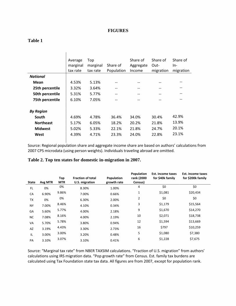
Inter-regional migration trends have been fairly consistent over the past three decades
(Table 1). In terms of aggregate flows, there has been a small but consistent outflow of
population and wealth from the Northeast region to the South since the 1980s. Table 1 compares
state migration figures, average regional income tax rates, and other regional characteristics.
The Northeast region faced disproportionately strong out-migration relative to its share of
the U.S. population, while having the highest average and top marginal tax rates out of the four
major geographic regions. The South and West, with the lowest tax rates, had disproportionately
higher in-migration (and lower out-migration). Table 2 lists the top ten states by total in-
migration in 2007. Cumulatively, migration into these “destination” states accounted for roughly
half of the total interstate movement in the U.S. in that year.
The data suggest that migrants tended to favor low tax states. Two of the top 10
destination states levied no income tax, Florida and Texas. Five of the destination states have
average marginal tax rates that rank in the lowest quartile of all states. The results correspond
with findings by Conway and Houtenville (2003) and the Pew Research Center (2008), which
found a positive net population flow from the Northeast and Midwest to the South in the 1990s
and 2000s. In the Pew Center’s ranking of “magnet states” (states with the highest percentage of
current state population born in another state), four of the top five magnet states were zero tax
states. We also note that people tended to move to states with bigger populations: the top four
states for in-migration flows are also the four most populous states.
We are particularly interested in New Jersey, because of its steady out-migration flow
over the past 25 years—a trend that has been attributed to the state’s relatively high tax rates,
high cost of living, and the decline of manufacturing in the Northeast (Laffer and Moore 2009,
Ebeling 2010). This is reflected in New Jersey’s low population growth rate over the past 30
years, relative to the national growth rate. Based on U.S. Census estimates, New Jersey’s
population grew 22.7% between 1970 and 2010, while the U.S. population grew 51.9%. As a
result, New Jersey’s share of the national U.S. population declined from a high of 3.5% in 1970
to 2.85% in 2010.
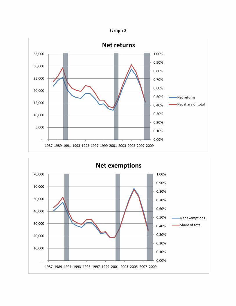
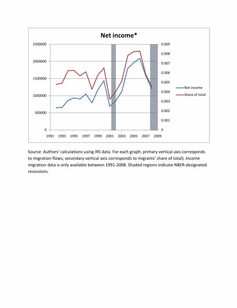
In Graph 2, we track net out-migration flows for New Jersey from 1988 to 2008 using the
IRS data. Taxpayer and exemption flows are available from 1988-2008; income flows are
available from 1992-2008. The graph shows that movements of taxpayers and income are highly
correlated: migration peaks in 2005, the year following the introduction of New Jersey’s
“millionaires’ tax.” By 2009, the share and overall levels of migrants had fallen by 50%.
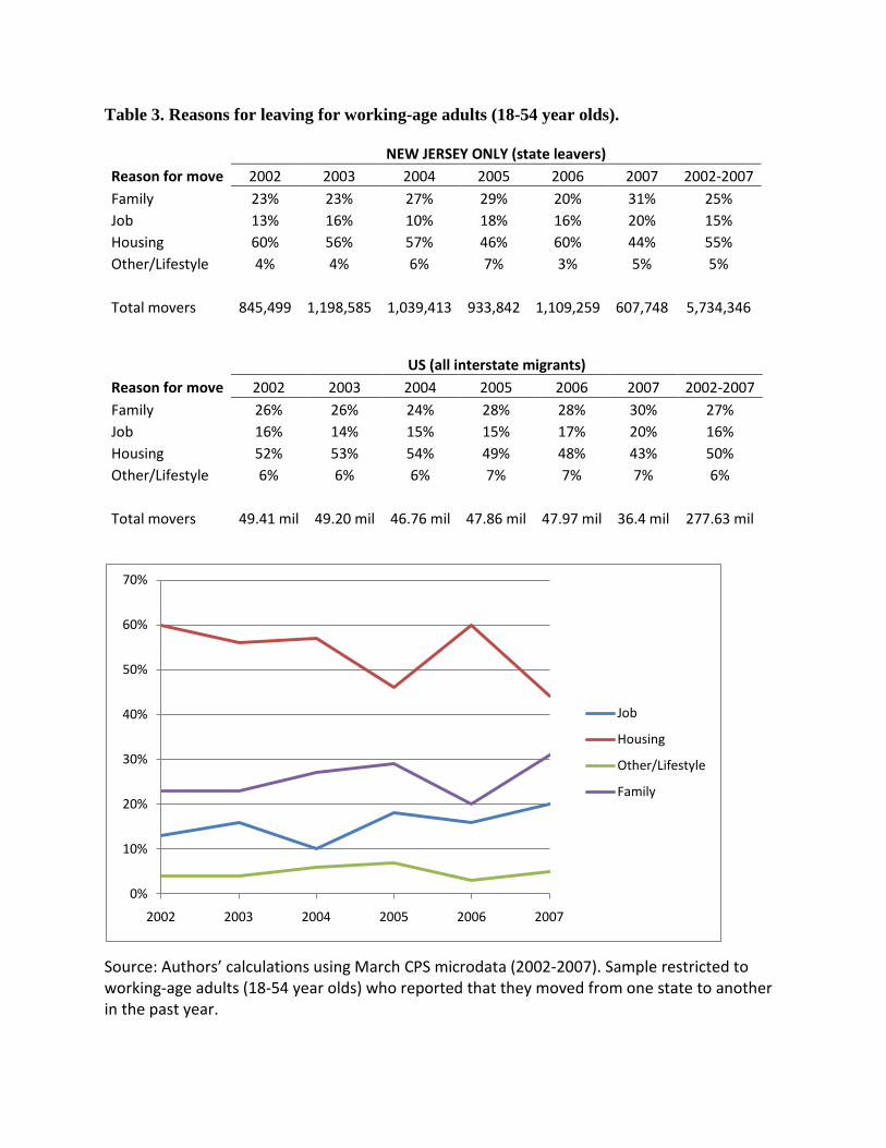
Understanding why individuals move is equally important, but notoriously difficult to pin
down. The Current Population Survey (CPS), administered by the Census Bureau, asks
respondents about their primary reason for moving. 4
However, housing concerns apparently played a major role in relocation decisions.
Between 2002 and 2007, more than 50% of respondents (New Jersey and national) listed a
housing-related issue as their primary reason for moving. The Young-Varner study attributed the
surge in out-migration to the 2003-2007 housing market boom. However, upon closer inspection,
the CPS results do not appear to support this claim. The fraction of housing-motivated migration
in the U.S. remains relatively consistent over time—in fact, it dips slightly from 53% in 2003 to
48% in 2006. For New Jersey movers, the percentage of housing-related moves fluctuates from
57% in 2004 to 46% in 2005 to 60% in 2006. While the CPS results suggest that housing costs
In Table 3, we break down reasons for
moving for working-age adults (ages 18-54). We compare responses from New Jersey migrants
(those people who moved out of New Jersey to another state in the past year) to responses from
all domestic migrants (those who moved from one state to another in the past year). The Census
did not ask respondents if they moved for tax reasons, and so we cannot determine tax effects
from these data.
4 Note that secondary reasons for moving would not be captured by the Current Population Survey.
are obviously a major factor for migration, the annual fluctuations appear unlikely to account for
the step-up in net outmigration from New Jersey in the last decade.
Young and Varner also attribute much of the “tax flight” effect to out-migration of
retirees to warmer locales. However, only 1-2% of respondents (both nationally and in New
Jersey) cited retirement as their primary reason for moving. Given these results, we believe that
other forces, such as varying changes in interstate tax differentials, may account for at least some
of the observed variation in migration movements, both in the CPS and IRS data.
III. Data and Theoretical Model
We model interstate migration decisions using logarithmic and standard linear regression
models5. For simplicity, we use the coefficients from the linear regression model to estimate
migration effects in Section IV. In both models, individuals are assumed to choose the state that
maximizes their predicted return, given a finite number of destinations. We also assume that an
individual decision-maker compares prospective destination states to the origin state in pair-wise
fashion; an individual bases his migration decision on differences in state characteristics6
where the Z variables are the expected return of moving to a destination state. The probability is
normalized by ∑k exp(Zikt), so that individual probabilities for a given year sum to one. The “out-
migration ratio” is defined as the probability that an individual will migrate from state i to state j,
5 This model is based on the theoretical framework presented in Gabriel et al. (1992) and Sasser (2010), 6 The logit model assumes Independence of Irrelevant Alternatives (IIA, which implies that error terms are independent and identically distributed. As a result, the model assumes that given a choice set of two states A and B, the addition of an alternative state C has no impact on the ratio of migration probabilities pi/pj. For a more detailed discussion of the multinomial logit model and its weaknesses, see Lattin et al. 2003.
divided by the probability that an individual will choose to stay in original state i. Taking the
natural log of the out-migration ratio, we arrive at the “log-odds ratio” that is used in the logit
Our analysis uses IRS state-to-state migration flow data from April 1992 to March 2009.
The IRS matched federal tax returns of filers across consecutive years using Social Security
numbers, and were thus able to track the aggregate flow of tax returns and income across state
lines7
This study contributes to the existing literature by calculating the direct effects of tax
policy on state-level migration. To the best of our knowledge, this is the first attempt to study the
marginal tax rate effects using IRS migration data. Since the dataset is based on tax filings, non-
filers (e.g., poor, college students) will almost certainly be underrepresented. However, in
comparing 20 years of IRS data with contemporaneous CPS data, Molloy et al. (2011) found no
significant differences in migration trends over time. In any case, since we are most interested in
studying tax effects on top earners, the omission of non-filers from the dataset would likely have
little impact.
. A distinct advantage of the rich IRS dataset is that it records gross in- and out-migration,
rather than net migration flows.
In both models, we estimate the effects of marginal tax rates on migration, controlling for
labor market conditions, housing costs, and other state-specific attributes. Based on our
7 Although counts of exemptions were included in the IRS migration data, we elected not to use them as a measure of out-migration. Individuals can claim additional exemptions when they meet certain criteria (e.g., being blind, elderly), and so the number of exemptions on a given tax return may exceed the actual number of people in a family. Admittedly, our use of tax returns to represent “families” may also lead to over-counting; for example, if a couple filed separate tax returns, they would be counted as two families. However, when we rerun the model using exemptions as the dependent variable, the magnitude or sign of the coefficients did not change significantly.
regressions estimates, we predict how changes in the marginal tax affect population and income
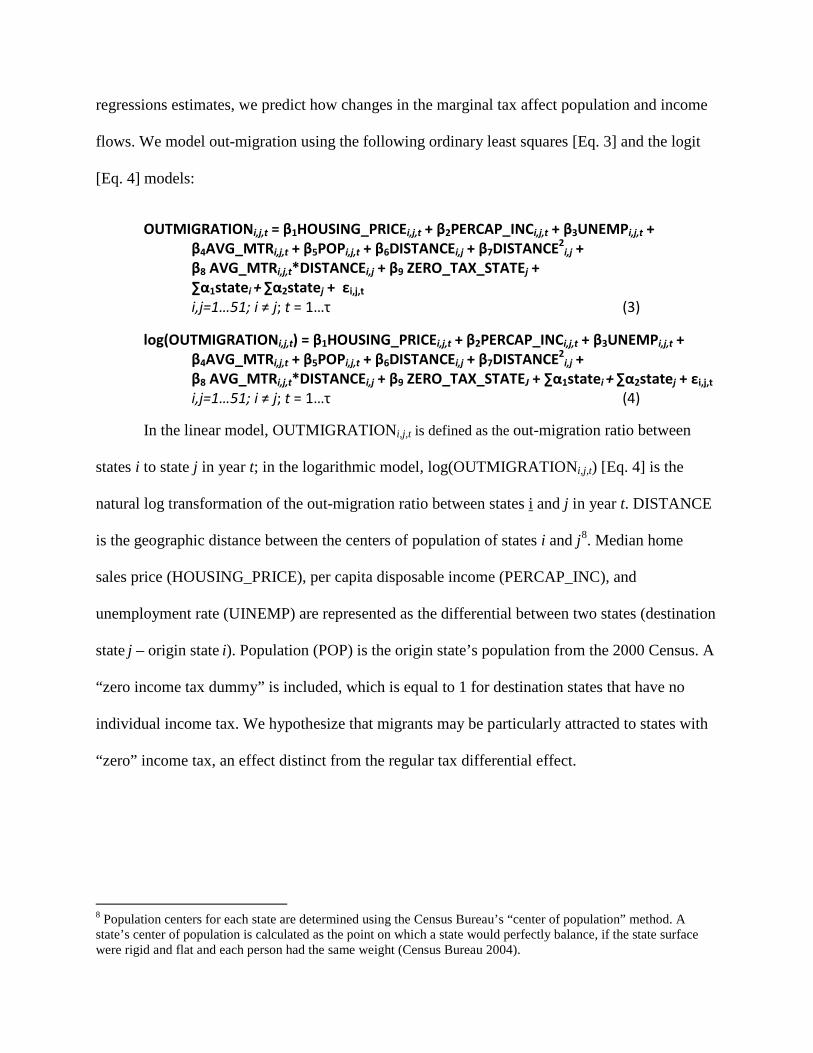
flows. We model out-migration using the following ordinary least squares [Eq. 3] and the logit
In the linear model, OUTMIGRATIONi,j,t is defined as the out-migration ratio between
states i to state j in year t; in the logarithmic model, log(OUTMIGRATIONi,j,t) [Eq. 4] is the
natural log transformation of the out-migration ratio between states i and j in year t. DISTANCE
is the geographic distance between the centers of population of states i and j8
8 Population centers for each state are determined using the Census Bureau’s “center of population” method. A state’s center of population is calculated as the point on which a state would perfectly balance, if the state surface were rigid and flat and each person had the same weight (Census Bureau 2004).
. Median home
sales price (HOUSING_PRICE), per capita disposable income (PERCAP_INC), and
unemployment rate (UINEMP) are represented as the differential between two states (destination
state j – origin state i). Population (POP) is the origin state’s population from the 2000 Census. A
“zero income tax dummy” is included, which is equal to 1 for destination states that have no
individual income tax. We hypothesize that migrants may be particularly attracted to states with
“zero” income tax, an effect distinct from the regular tax differential effect.
Average marginal tax rates were obtained from NBER’s TAXSIM model, and reflect
cross-deductibility of federal and state taxes when appropriate9
IV. Regression results
. To control for state amenities
and other state-specific features, the model includes origin and destination state fixed effects
(statei , statej). Since each state (and the District of Columbia) can be either an origin or a
destination state, there are a total of 102 fixed effects. We omit year fixed effects from the
regressions, because they are not jointly significant in any of the specifications. To avoid
potential simultaneity issues, we use 1-period lagged values of housing prices, per capita income,
unemployment rate, and average marginal tax rate.
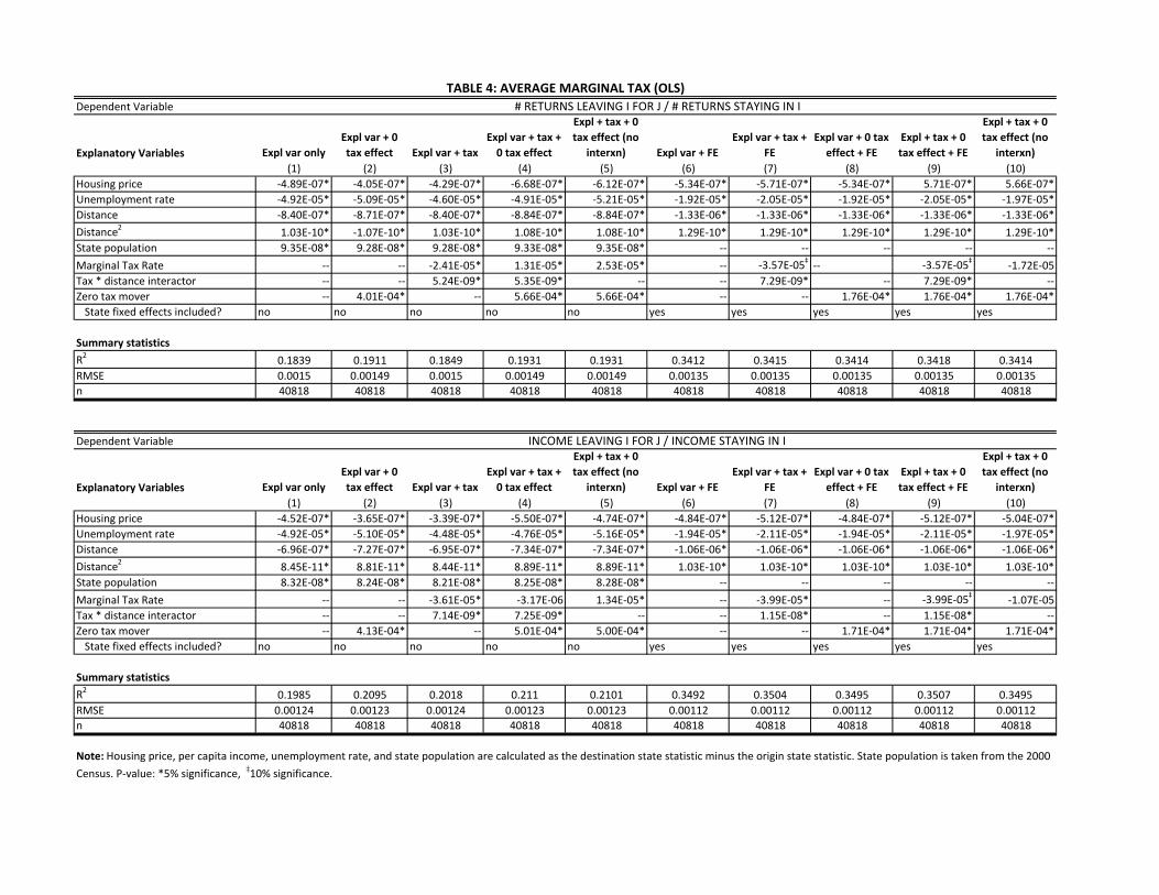
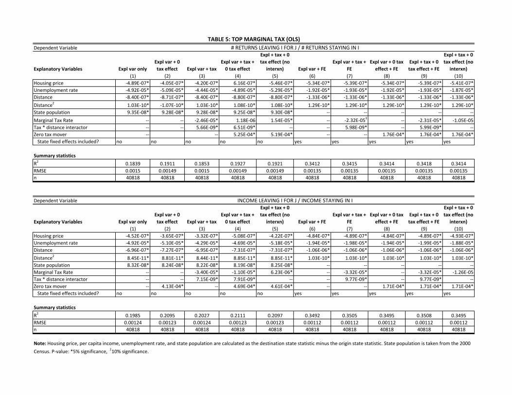
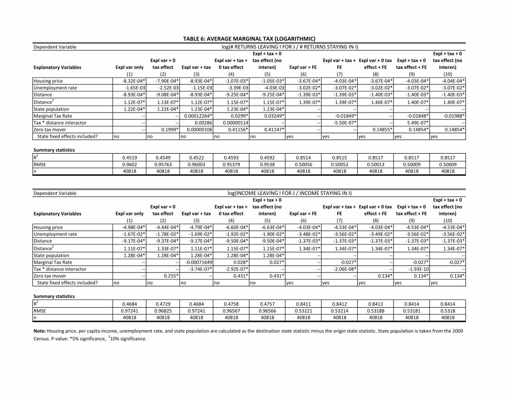
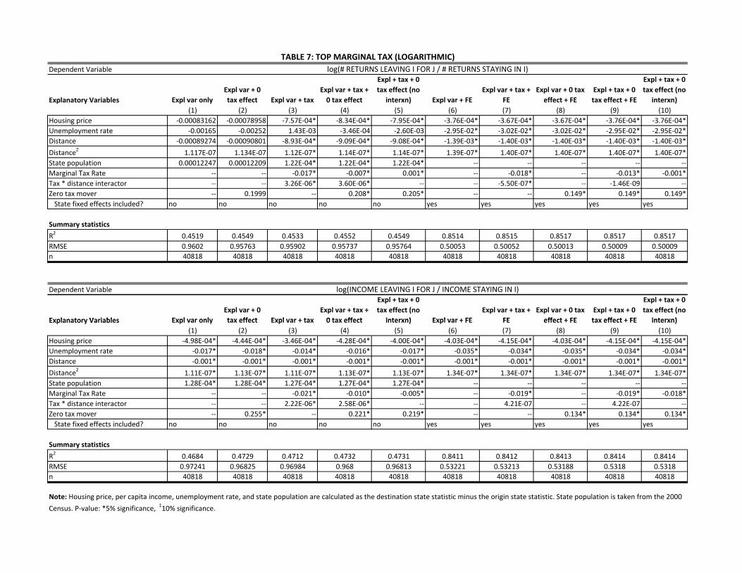
We report the linear regression results in Tables 4 and 5, and the logarithmic regression
results in Tables 6 and 7. We measure migration flow (the dependent variable) using two
different measures, movement of taxpayers (top panel) and movement of income (bottom panel).
The returns out-migration ratio is defined as the total number of returns moving from state i to j
divided by the total number of returns originally in state i. Similarly, the income out-migration
ratio is calculated by dividing the total income moving from state i to j by the total income
originally in state i.
The model coefficient estimates are generally consistent with a priori expectations: in all
linear regressions, the average marginal tax rate coefficient is negatively signed. This indicates
that out-migration is greater when the originating state’s average marginal tax rate is higher than
the destination state’s. The logarithmic model results are less readily interpretable: the
coefficient on average marginal tax is negative and significant only when state fixed effects are
9 Note that local income taxes (county, city taxes) are not taken into account. For example, New York City’s individual income tax would not be reflected in the calculated New York state tax.
included. In both linear and logit models, the coefficient for “zero income tax” states is
positively significant for all regressions in which the dummy is included. This suggests that
individuals have a strong preference for zero income tax states. State fixed effects are highly
significant in all regressions.
In both tables, the coefficients also indicate that higher housing prices and higher
unemployment rate lead to greater out-migration. As expected, greater geographic distance
between two states weakens the tax effect: the positive coefficient on the tax*distance
interaction term indicates residents are less sensitive to cross-state tax differentials the further a
potential state lies from the originating state. Also, we also find the large state effect observed in
Census data by Perry 2003: states with large populations are more likely to receive migrants
from other states.
V. Calculations
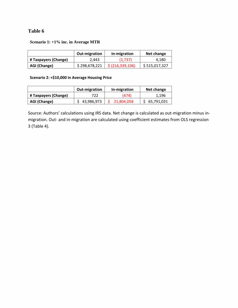
From the regression results in Table 6, we estimate changes in population and income
losses for two scenarios, using New Jersey as our test case. Under the first scenario, New Jersey
raises its average marginal state income tax rates by 1 percentage point. As an “across the board”
tax increase, a 1 percentage point raise would be a very large tax hike that is more than twice as
large as the actual 2004 “millionaires’ tax.” Under the second scenario, average housing prices in
New Jersey rise by $10,000. For simplicity, we hold all other factors constant in each scenario.
Based on internal NJ Treasury projections, we estimate that a one percentage point
increase would raise roughly $2.5 billion in additional tax revenue. However, this figure would
be partially offset and eroded over time by out- and in-migration effects. Our model suggests that
New Jersey would see increased annual net outflows of about 4,200 taxpayers and $530 million
of AGI. Income losses would translate to roughly $29 million in lost income tax revenue for the
state. By dividing the estimated loss of AGI by the number of lost taxpayers, we estimate that the
state would lose an average of roughly $125,000 in income per lost taxpayer, almost double New
Jersey’s 2009 median household income of $68,000. This suggests that tax increases are
associated with increased out-migration (or lessened in-migration) of upper-income taxpayers.
The model shows an association between higher home prices and higher net migration,
which is consistent with the CPS findings. In the second scenario, we estimate that a $10,000
increase in New Jersey home prices would have a modest effect on migration: on net, New
Jersey would lose a total of 1200 taxpayers and $66 million in AGI. It is difficult to compare this
directly with the tax rate effect, but the housing effect seems relatively smaller and, given the
volatility of home prices, would probably be short-lived.
Finally, we estimated the cumulative effect of New Jersey tax changes since 2003. These
changes include the 2004 and temporary 2009 legislated tax hikes, as well as the impact of
bracket creep. Had tax rates remained at 2003 levels, we predict that New Jersey would have had
roughly 20,000 more taxpayers in 2009. Also, AGI would have been $2.4 billion higher,
generating more than $125 million in additional state income tax. Based on the average losses for
2004-2009, we believe that by 2011 the cumulative loss in taxpayers was over 25,000, the loss in
AGI was roughly $3 billion, and the annual shortfall in state income tax revenue was greater than
$150 million, which amounts to a substantive portion of the incremental revenue (a bit over $1
billion) directly attributable to the 2004 rate increase.
VI. Conclusion
This paper analyzes the effects of state marginal tax rates on domestic migration in the
U.S. between tax years 1992 and 2008. Using IRS migration data, we calculated the specific
state-to-state migration flows of taxpayers and income for every year and state pair. We find that
average marginal tax rates had a small but significant effect on migration decisions in the U.S.
and in New Jersey. We estimate that higher New Jersey income taxes after 2003 was associated
with a reduction of more than 20,000 taxpayers and a loss of annual income of at least $2 1/2
billion.
Clearly, our results do not suggest that tax-induced migration would come anywhere
close to eclipsing the immediate revenue gain from an income tax increase, but losses would
cumulate over time. Our analysis of the New Jersey 2004 “millionaires’ tax” suggests that over
time migration effects could offset a meaningful share of the revenue boost. Additionally, out-
migration associated with higher income taxes will likely diminish other streams of state
revenue, such as corporate tax, sales tax, and property tax, as well as degrade a state’s overall
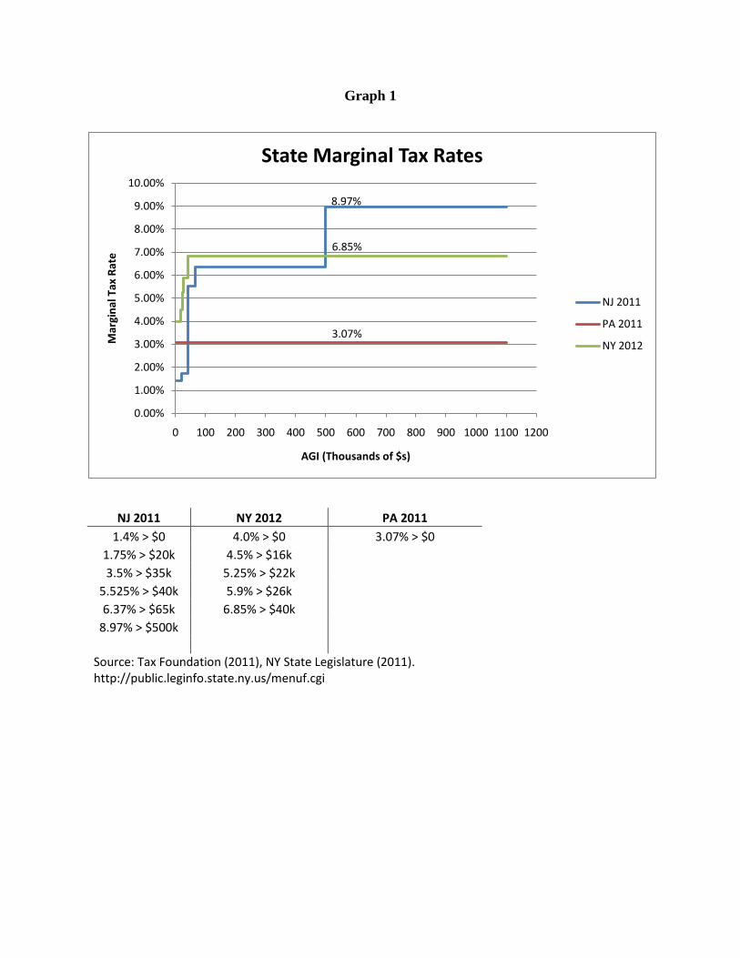
economic performance, in turn associated with further out-migration. Given New York’s 2012
reduction in income taxes, it seems sensible that New Jersey legislators should keep in mind the
potential impact of New Jersey taxes on migration. By January 1, 2012 (when New York’s lower
top marginal tax rate takes effect), Garden State households making more than $500,000 in AGI
will face the highest top marginal tax rate in the tri-state area: New Jersey households will be
taxed at 8.97%, compared to New York’s 6.85% marginal tax rate and Pennsylvania’s 3.07% flat
tax rate.
There are a number of limitations in using the IRS data. Since migration flows are
aggregated, it is impossible to determine how different groups of taxpayers react to tax policy. A
policymaker considering an introduction of a “millionaire’s tax” would probably be most
interested in learning specifically how top earners react to tax increases at the top brackets, rather
than how the general population responds. A disproportionately strong out-migration could
significantly offset gains in tax revenue. With micro-level data, we could track movements of
taxpayers over time, and control for unobserved individual characteristics that could influence
migration decisions (e.g., age, race, education), as well as explore the interaction of income and
estate taxes on migration.
Without further exploration, it is certainly possible to argue that the connection we draw
is not causal: independent forces could simultaneously spur out-migration from a state and
impose sufficient fiscal stress to trigger tax hikes. Our attempt to control for this through state
fixed effects and observed economic circumstances may not be sufficient. In any event, our
results appear to suggest a meaningful association between state taxes and migration.
FIGURES
Table 1
Average marginal tax rate
Top marginal tax rate
Share of Population
Share of Aggregate Income
Share of Out-migration
Share of In-migration
National
Mean 4.53% 5.13% -- -- -- --
25th percentile 3.32% 3.64% -- -- -- --
50th percentile 5.31% 5.77% -- -- -- --
75th percentile 6.10% 7.05% -- -- -- --
By Region
South 4.69% 4.78% 36.4% 34.0% 30.4% 42.9%
Northeast 5.17% 6.05% 18.2% 20.2% 21.8% 13.9%
Midwest 5.02% 5.33% 22.1% 21.8% 24.7% 20.1%
West 4.39% 4.71% 23.3% 24.0% 22.8% 23.1%
Source: Regional population share and aggregate income share are based on authors’ calculations from 2007 CPS microdata (using person weights). Individuals traveling abroad are omitted.
Table 2. Top ten states for domestic in-migration in 2007.
State Avg MTR Top MTR
Fraction of total U.S. migration
Population growth rate
Population rank (2000
Census)
Est. income taxes for $40k family
Est. income taxes for $200k family
FL 0% 0% 8.30% 1.00% 4 $0 $0
CA 6.90% 9.86% 7.00% 0.66% 1 $1,081 $20,434
TX 0% 0% 6.30% 2.00% 2 $0 $0
NY 7.00% 8.46% 4.10% 0.34% 3 $1,179 $15,564
GA 5.60% 5.77% 4.00% 2.18% 9 $1,670 $14,270
NC 7.08% 8.16% 4.00% 2.19% 10 $2,071 $18,738
VA 5.70% 5.78% 3.80% 0.94% 12 $1,594 $13,669
AZ 3.19% 4.43% 3.30% 2.73% 16 $797 $10,259
IL 3.00% 3.00% 3.20% 0.48% 5 $1,080 $7,380
PA 3.10% 3.07% 3.10% 0.41% 6 $1,228 $7,675
Source: “Marginal tax rate” from NBER TAXSIM calculations. “Fraction of U.S. migration” from authors’ calculations using IRS migration data. “Pop growth rate” from Census. Est. family tax burdens are calculated using Tax Foundation state tax data. All figures are from 2007, except for population rank.
Graph 1
NJ 2011 NY 2012 PA 2011 1.4% > $0 4.0% > $0 3.07% > $0
Source: Authors’ calculations using IRS data. For each graph, primary vertical axis corresponds to migration flows; secondary vertical axis corresponds to migrants’ share of total). Income migration data is only available between 1991-2008. Shaded regions indicate NBER-designated recessions.
0
0.001
0.002
0.003
0.004
0.005
0.006
0.007
0.008
0.009
0
500000
1000000
1500000
2000000
2500000
1991 1993 1995 1997 1999 2001 2003 2005 2007 2009
Net income*
Net income
Share of total
Table 3. Reasons for leaving for working-age adults (18-54 year olds).
Total movers 49.41 mil 49.20 mil 46.76 mil 47.86 mil 47.97 mil 36.4 mil 277.63 mil
Source: Authors’ calculations using March CPS microdata (2002-2007). Sample restricted to working-age adults (18-54 year olds) who reported that they moved from one state to another in the past year.
0%
10%
20%
30%
40%
50%
60%
70%
2002 2003 2004 2005 2006 2007
Job
Housing
Other/Lifestyle
Family
Dependent Variable
Explanatory Variables Expl var onlyExpl var + 0 tax effect Expl var + tax
Note: Housing price, per capita income, unemployment rate, and state population are calculated as the destination state statistic minus the origin state statistic. State population is taken from the 2000
TABLE 5: TOP MARGINAL TAX (OLS)# RETURNS LEAVING I FOR J / # RETURNS STAYING IN I
INCOME LEAVING I FOR J / INCOME STAYING IN I
Explanatory Variables Expl var only tax effect Expl var + tax 0 tax effect interxn) Expl var + FE FE effect + FE tax effect + FE interxn)(1) (2) (3) (4) (5) (6) (7) (8) (9) (10)
Note: Housing price, per capita income, unemployment rate, and state population are calculated as the destination state statistic minus the origin state statistic. State population is taken from the 2000
Note: Housing price, per capita income, unemployment rate, and state population are calculated as the destination state statistic minus the origin state statistic. State population is taken from the 2000
Explanatory Variables Expl var onlyExpl var + 0 tax effect Expl var + tax
Expl var + tax + 0 tax effect
Expl + tax + 0 tax effect (no
interxn) Expl var + FEExpl var + tax +
FEExpl var + 0 tax effect + FE
Expl + tax + 0 tax effect + FE
Expl + tax + 0 tax effect (no
interxn)
TABLE 7: TOP MARGINAL TAX (LOGARITHMIC)log(# RETURNS LEAVING I FOR J / # RETURNS STAYING IN I)
log(INCOME LEAVING I FOR J / INCOME STAYING IN I)
Explanatory Variables Expl var only tax effect Expl var + tax 0 tax effect interxn) Expl var + FE FE effect + FE tax effect + FE interxn)(1) (2) (3) (4) (5) (6) (7) (8) (9) (10)
Note: Housing price, per capita income, unemployment rate, and state population are calculated as the destination state statistic minus the origin state statistic. State population is taken from the 2000
Source: Authors’ calculations using IRS data. Net change is calculated as out-migration minus in-migration. Out- and in-migration are calculated using coefficient estimates from OLS regression 3 (Table 4).
References
Bakija, J. & Slemrod, J.. 2004. Do the Rich Flee from High State Taxes? Evidence from Federal
Estate Tax Returns. National Bureau of Economic Research, Cambridge, MA. Working
Paper #10645.
Borjas, G., Bronars, S., & Trejo, S. 1992. Self-selection and internal migration in the United
States. Journal of Urban Economics 32(2), 159-185.
Carlino, G. & Milles, E. (1987). The Determinants of County Growth. Journal of Regional
Science. 27(1), 39-54.
Clark, D., & Hunter, W. The impact of economic opportunity, amenities and fiscal factors of
age-specific migration rates. Journal of Regional Science 32(3), 349-365.
Conway, K., & Houtenville, A. (2003). Out with the Old, In with the Old: A Closer Look at
Younger Versus Older Elderly Migration. Social Science Quarterly 84(2), 309-328.
Coomes, P., & Hoyt, W. Income taxes and the destination of movers to multistate MSAs.
Journal of Urban Economics 63(3), 920-937.
Diulio, N. (2011, May 20). Christie: New Jersey must sustain fiscal discipline. Princeton