American Economic Review 2017, 107(1): 217–248 https://doi.org/10.1257/aer.20140855 217 Tax Policy and Heterogeneous Investment Behavior † By Eric Zwick and James Mahon* We estimate the effect of temporary tax incentives on equipment investment using shifts in accelerated depreciation. Analyzing data for over 120,000 firms, we present three findings. First, bonus depre- ciation raised investment in eligible capital relative to ineligible cap- ital by 10.4 percent between 2001 and 2004 and 16.9 percent between 2008 and 2010. Second, small firms respond 95 percent more than big firms. Third, firms respond strongly when the policy generates immediate cash flows, but not when cash flows only come in the future. This heterogeneity materially affects investment-weighted esti- mates and supports models in which financial frictions or fixed costs amplify investment responses. (JEL D21, D22, D92, G31, H25, H32) Economists have long asked how taxes affect investment (Hall and Jorgenson 1967). The answer is central to the design of countercyclical fiscal policy, since pol- icymakers often use tax-based investment incentives to spur growth in times of eco- nomic weakness. Improving policy design requires knowing which firms are most responsive to taxes and why they respond. However, because comprehensive micro data have been previously unavailable, past work has not fully explored the role of heterogeneity in how tax policy affects investment or whether such heterogeneity is macroeconomically relevant. 1 1 Key theoretical studies include Hall and Jorgenson (1967); Tobin (1969); Hayashi (1982); Abel and Eberly (1994); and Caballero and Engel (1999). Abel (1990) presents a unifying synthesis of the early theoretical lit- erature. Key empirical work includes Summers (1981); Auerbach and Hassett (1992); Cummins, Hassett, and Hubbard (1994); Goolsbee (1998); Chirinko, Fazzari, and Meyer (1999); Desai and Goolsbee (2004); Cooper and Haltiwanger (2006); House and Shapiro (2008); and Yagan (2015). Edgerton (2010) explores heterogeneity within a sample of public companies but finds mixed results. * Zwick: University of Chicago Booth School of Business, 5807 S. Woodlawn Avenue, Chicago, IL, 60637, and NBER (e-mail: [email protected]); Mahon: Deloitte LLP (e-mail: [email protected]). This paper previously circulated with the title, “Do Financial Frictions Amplify Fiscal Policy? Evidence from Business Investment Stimulus.” Zwick thanks Raj Chetty, David Laibson, Josh Lerner, David Scharfstein, and Andrei Shleifer for extensive advice and support. We thank Jediphi Cabal, Gary Chamberlain, George Contos, Ian Dew-Becker, Fritz Foley, Paul Goldsmith-Pinkham, Robin Greenwood, Sam Hanson, Ron Hodge, John Kitchen, Pat Langetieg, Day Manoli, Isaac Sorkin, Larry Summers, Adi Sunderam, Nick Turner, Tom Winberry, Danny Yagan, Moto Yogo, Owen Zidar, and seminar and conference participants for comments, ideas, and help with data. Tom Cui and Prab Upadrashta provided excellent research assistance. We are grateful to our colleagues in the US Treasury Office of Tax Analysis and the IRS Office of Research, Analysis, and Statistics—especially Curtis Carlson, John Guyton, Barry Johnson, Jay Mackie, Rosemary Marcuss, and Mark Mazur—for making this work possible. The views expressed here are ours and do not necessarily reflect those of the US Treasury Office of Tax Analysis, nor the IRS Office of Research, Analysis, and Statistics. Zwick gratefully acknowledges financial support from the Harvard Business School Doctoral Office, the Neubauer Family Foundation, and Booth School of Business at the University of Chicago. The authors declare that they have no relevant or material financial interests that relate to the research described in this paper. † Go to https://doi.org/10.1257/aer.20140855 to visit the article page for additional materials and author disclosure statement(s).
Transcript
American Economic Review 2017, 107(1): 217–248 https://doi.org/10.1257/aer.20140855
217
Tax Policy and Heterogeneous Investment Behavior†
By Eric Zwick and James Mahon*
We estimate the effect of temporary tax incentives on equipment investment using shifts in accelerated depreciation. Analyzing data for over 120,000 firms, we present three findings. First, bonus depre-ciation raised investment in eligible capital relative to ineligible cap-ital by 10.4 percent between 2001 and 2004 and 16.9 percent between 2008 and 2010. Second, small firms respond 95 percent more than big firms. Third, firms respond strongly when the policy generates immediate cash flows, but not when cash flows only come in the future. This heterogeneity materially affects investment-weighted esti-mates and supports models in which financial frictions or fixed costs amplify investment responses. (JEL D21, D22, D92, G31, H25, H32)
Economists have long asked how taxes affect investment (Hall and Jorgenson 1967). The answer is central to the design of countercyclical fiscal policy, since pol-icymakers often use tax-based investment incentives to spur growth in times of eco-nomic weakness. Improving policy design requires knowing which firms are most responsive to taxes and why they respond. However, because comprehensive micro data have been previously unavailable, past work has not fully explored the role of heterogeneity in how tax policy affects investment or whether such heterogeneity is macroeconomically relevant.1
1 Key theoretical studies include Hall and Jorgenson (1967); Tobin (1969); Hayashi (1982); Abel and Eberly (1994); and Caballero and Engel (1999). Abel (1990) presents a unifying synthesis of the early theoretical lit-erature. Key empirical work includes Summers (1981); Auerbach and Hassett (1992); Cummins, Hassett, and Hubbard (1994); Goolsbee (1998); Chirinko, Fazzari, and Meyer (1999); Desai and Goolsbee (2004); Cooper and Haltiwanger (2006); House and Shapiro (2008); and Yagan (2015). Edgerton (2010) explores heterogeneity within a sample of public companies but finds mixed results.
* Zwick: University of Chicago Booth School of Business, 5807 S. Woodlawn Avenue, Chicago, IL, 60637, and NBER (e-mail: [email protected]); Mahon: Deloitte LLP (e-mail: [email protected]). This paper previously circulated with the title, “Do Financial Frictions Amplify Fiscal Policy? Evidence from Business Investment Stimulus.” Zwick thanks Raj Chetty, David Laibson, Josh Lerner, David Scharfstein, and Andrei Shleifer for extensive advice and support. We thank Jediphi Cabal, Gary Chamberlain, George Contos, Ian Dew-Becker, Fritz Foley, Paul Goldsmith-Pinkham, Robin Greenwood, Sam Hanson, Ron Hodge, John Kitchen, Pat Langetieg, Day Manoli, Isaac Sorkin, Larry Summers, Adi Sunderam, Nick Turner, Tom Winberry, Danny Yagan, Moto Yogo, Owen Zidar, and seminar and conference participants for comments, ideas, and help with data. Tom Cui and Prab Upadrashta provided excellent research assistance. We are grateful to our colleagues in the US Treasury Office of Tax Analysis and the IRS Office of Research, Analysis, and Statistics—especially Curtis Carlson, John Guyton, Barry Johnson, Jay Mackie, Rosemary Marcuss, and Mark Mazur—for making this work possible. The views expressed here are ours and do not necessarily reflect those of the US Treasury Office of Tax Analysis, nor the IRS Office of Research, Analysis, and Statistics. Zwick gratefully acknowledges financial support from the Harvard Business School Doctoral Office, the Neubauer Family Foundation, and Booth School of Business at the University of Chicago. The authors declare that they have no relevant or material financial interests that relate to the research described in this paper.
† Go to https://doi.org/10.1257/aer.20140855 to visit the article page for additional materials and author disclosure statement(s).
218 THE AMERICAN ECONOMIC REVIEW JANuARy 2017
This paper uses two episodes of investment stimulus and a difference-in-differences methodology to study the effect of taxes on investment and how it varies across firms. The policy we study, “bonus” depreciation, accelerates the schedule for when firms can deduct from taxable income the cost of investment purchases. Bonus alters the timing of deductions but not their amount, so the economic incentive created by bonus works because future deductions are worth less than current deductions. That is, bonus works because of discounting: firms judge the benefits of bonus by the present discounted value of deductions over time.2
Our first empirical finding is that bonus depreciation has a substantial effect on investment. Across firms with differential exposure to bonus, we find a rela-tive investment response of 10.4 percent on average between 2001 and 2004, and 16.9 percent between 2008 and 2010. Our estimates are consistent with the large response House and Shapiro (2008) document for the first episode of bonus, but well above estimates from studies of other tax reforms.3
The first part of the paper details this finding and a litany of robustness tests. The research design compares firms at the same point in time whose benefits from bonus differ. Our strategy exploits technological differences between firms in narrowly defined industries. Firms in industries with most of their investment in short dura-tion categories act as the “control group” because bonus only modestly alters their depreciation schedule. This natural experiment separates the effect of bonus from other economic shocks happening at the same time. If the parallel trends assump-tion holds—if investment growth for short- and long-duration industries would have been similar absent the policy—then the experimental design is valid.4
The key threat to this design is that time-varying industry shocks may coin-cide with bonus. This risk is limited for four reasons. First, graphical inspection of parallel trends indicates smooth pretrends and a clear, steady break short- and long-duration firms during both the 2001 to 2004 and 2008 to 2010 bonus periods. The effects are the same size in both periods, though different industries suffered in each recession. Second, the estimates are stable across many specifications and after including firm-level cash flow controls, industry Q, and flexible industry trends. Controlling for industry-level co-movement with the macroeconomy increases our estimates, and we confirm parallel trends in past recessions when policymakers did not introduce investment stimulus. Third, the estimates pass a placebo test: the effect of bonus on ineligible investment is indistinguishable from zero. Last, for firms making eligible investments, bonus take-up rates (i.e., whether firms fill in the bonus box on the tax form) are indeed higher in long-duration industries. For these rea-sons, spurious factors are unlikely to explain the large effect of bonus.
2 Summers (1987, p. 29.5) states this most clearly: “It is only because of discounting that depreciation schedules affect investment decisions”
3 Cummins, Hassett, and Hubbard (1994) study many corporate tax reforms with public company data and conclude that tax policy has a strong effect on investment. Using similar data and a different empirical methodol-ogy, Chirinko, Fazzari, and Meyer (1999) argue that tax policy has a small effect on investment and that Cummins, Hassett, and Hubbard (1994) misinterpret their results. Hassett and Hubbard (2002) survey empirical work and conclude that the range of estimates for the user cost elasticity has narrowed to between −0.5 and −1. Surveying this and more recent work, Bond and Van Reenen (2007, p. 4473) decide “it is perhaps a little too early to agree with Hassett and Hubbard (2002) that there is a new ‘consensus’ on the size and robustness of this effect.”
4 The research design relies on cross-sectional program exposure. Thus, the estimates do not reveal the overall general equilibrium effects of the program, which are subsumed into time fixed effects and would include, for example, price changes and their effect on the aggregate level of investment.
219Zwick and Mahon: Tax Policy and invesTMenT Behaviorvol. 107 no. 1
In the second part of the paper, we present a set of heterogeneity tests designed to shed light on the mechanisms underlying the large baseline response. Our second empirical finding is that small firms are substantially more responsive to investment stimulus. We work with an analysis sample of more than 120,000 public and private companies drawn from two million corporate tax returns. Half the firms in our sam-ple are smaller than the smallest firms in Compustat.5 The largest firms in our sam-ple, those most like the public company samples from prior work, yield estimates in line with past studies of other tax reforms. In contrast, small and medium-sized firms show much stronger responses. Though aggregate investment is concentrated at the top of the firm size distribution—the top 5 percent of firms in our sample account for more than 60 percent of investment—accounting for the bottom 95 percent of firms materially affects our investment-weighted estimate. The investment-weighted elas-ticity is 2.89, which is 27 percent higher than the 2.27 estimated using only the largest firms.
The asymmetry of the corporate tax code introduces another source of heteroge-neity: firms with tax losses must wait to realize the benefits of tax breaks. Because many firms in our sample are in a tax loss position when a policy shock occurs, we can ask how much firms value future tax benefits, namely, the larger deductions bonus depreciation provides them in later years. Our third empirical finding is that firms only respond to investment incentives when the policy immediately generates cash flows. This finding holds even though firms can carry forward unused deduc-tions to offset future taxes, and it cannot be explained by differences in growth opportunities.
To confirm the importance of immediacy, we study a second component of the depreciation schedule. Firms making small investment outlays face a permanent kink in the tax schedule, which creates a discontinuous change in marginal invest-ment incentives. This sharp change in incentives induces substantial investment bunching, with many firms electing amounts within just a few hundred dollars of the kink. And when legislation raises the kink, the bunching pattern follows. Immediacy proves crucial in this setting, as bunching strongly depends on a firm’s current tax status: firms just in positive tax position are far more likely to bunch than firms on the other side of the discontinuity. For a different group of firms and a different depreciation policy, we again find that firms ignore future tax benefits.
Our findings have implications for which models of corporate behavior are most likely to fit the data. In the presence of financial frictions (Jensen and Meckling 1976; Myers and Majluf 1984; Stein 2003), firms value future cash flows with high effective discount rates, which amplify the perceived value of bonus incen-tives because the difference in today’s tax benefits dwarfs the present value com-parison that matters in frictionless models. Building on the differential response by firm size, we perform a split sample analysis using alternative markers of ex ante financial constraints. In addition to small firms, non-dividend payers and firms with low cash holdings are 1.5 to 2.6 times more responsive than their unconstrained
5 When aggregated, these small firms account for a large amount of economic activity. According to census tab-ulations in 2007, firms with less than $100 million in receipts (around the eightieth percentile in our data) account for more than half of total employment and one-third of total receipts (https://www.census.gov/epcd/susb/2007/us/US--.HTM).
220 THE AMERICAN ECONOMIC REVIEW JANuARy 2017
counterparts. Moreover, we find that firms respond by borrowing and cutting div-idends. That firms only respond to immediate tax benefits also suggests models in which liquidity considerations matter.
Though these facts suggest a role for financial frictions, markers of financial con-straints and tax position may also measure the likelihood of adjustment in models with non-convex adjustment costs (Caballero and Engel 1999; Cooper and Haltiwanger 2006). In these models, when the policy induces a firm across its adjustment thresh-old, investment increases sharply because the firm does not plan to adjust every year. Thus, models in which fixed costs lead firms to differ in their relative distance from an adjustment threshold may also explain the patterns we observe. Consistent with this idea, firms very likely or very unlikely to invest in the absence of the policy indeed exhibit lower elasticities. Taken together, the data point toward models in which finan-cial frictions, fixed costs, or a mix of these factors amplifies investment responses.
Our paper follows a long literature that exploits cross-sectional variation to study the effect of tax policy on investment (Cummins, Hassett, and Hubbard 1994; Goolsbee 1998; House and Shapiro 2008). We depart by using a broader sample of firms than public company samples and by using detailed micro data to pres-ent new heterogeneity analyses, which shed light on the underlying mechanisms. Allowing for heterogeneous responses also proves necessary to estimate an accurate investment-weighted elasticity. In addition, the results suggest that countercyclical policy aimed at high elasticity subpopulations can produce larger effects, in a simi-lar spirit to studies documenting heterogeneous responses of consumption to policy changes (Shapiro and Slemrod 1995; Johnson, Parker, and Souleles 2006; Aaronson, Agarwal, and French 2012). Our findings also highlight the potential importance of distinguishing tax policies that target investment directly and immediately—such as depreciation changes—from policies that more broadly affect the cost of capital and pay off gradually over time—such as corporate or dividend tax changes (Feldstein 1982; Auerbach and Hassett 1992; Yagan 2015).
Section I introduces the bonus depreciation policy and our conceptual approach. Section II describes the corporate tax data, variable construction, and sample selec-tion process. Section III describes the main empirical strategy for studying bonus depreciation, the identification assumptions, and presents results and robustness tests. Section IV explores the role of heterogeneity in driving our results and pres-ents investment-weighted estimates that account for this heterogeneity. Section V connects our findings to past work and discusses alternative theoretical interpreta-tions. Section VI concludes.
I. Bonus Depreciation
A. Conceptual Approach
Consider a firm buying $1 million worth of computers. The firm owes corporate taxes on income net of business expenses. For expenses on nondurable items such as wages and advertising, the firm can immediately deduct the full cost of these items on its tax return. Thus an extra dollar of spending on wages reduces the firm’s taxable income by a dollar and reduces the firm’s tax bill by the tax rate. But for investment expenses the rules differ.
221Zwick and Mahon: Tax Policy and invesTMenT Behaviorvol. 107 no. 1
Usually, the firm follows the regular depreciation schedule in the top panel of Table 1. The first year deduction is $200,000, which provides an after-tax benefit of $70,000. Over the next five years, the firm deducts the remaining $800,000. The total undiscounted deduction is the $1 million spent and the total undiscounted tax benefit is $350,000.
The value of these deductions thus depends on the tax rate and how the schedule interacts with the firm’s discount rate. We collapse the stream of future depreciation deductions owed for investment:
(1) z 0 = D 0 + ∑ t=1
T
1 _____ (1 + r) t D t ,
where D t is the allowable deduction per dollar of investment in period t , T is the class life of investment, and r is the risk-adjusted rate the firm uses to discount future flows. z 0 measures the present discounted value of one dollar of investment deductions before tax. If the firm can immediately deduct the full dollar, then z 0 equals one. Because of discounting, z 0 is lower for longer-lived items (i.e., items with greater T ), which forms the core of our identification strategy.
In general, the stream of future deductions depends on future discount rates and tax rates. For discount rates, we apply a risk-adjusted rate of 7 percent for r to compute z 0 in the data, which enables comparison to past work. Our empirical analysis assumes the effective tax rate does not change over time, except when the firm is nontaxable.6 When the next dollar of investment does not affect this year’s tax bill, then the firm must carry forward the deductions to future years.7
6 We use the top statutory tax rate in the set of specifications requiring a tax rate. This is an upper bound on the more realistic effective marginal tax rate, which in turn depends on tax rate progressivity and the level of other expenses relative to taxable income. See, e.g., Graham (1996, 2000) for a method tracing out the marginal tax benefit curve. The policies we study will increase the use of investment as a tax shield regardless of where the firm is on this marginal benefit curve. Except when current and all future taxes are zero, bonus increases the marginal tax benefit of investment.
7 This assumes that “carrybacks”—in which firms apply unused deductions this year against past tax bills—have been exhausted or ignored.
Table 1—Regular and Bonus Depreciation Schedules for Five-Year Items
Notes: This table displays year-by-year deductions and tax benefits for a $1 million investment in computers, a five-year item, depreciable according to the Modified Accelerated Cost Recovery System (MACRS). The top schedule applies during normal times. It reflects a half-year convention for the purchase year and a 200 percent declining balance method (2× straight line until straight line is greater). The bottom schedule applies when 50 percent bonus depreciation is available.
Source: Authors’ calculations. See IRS publication 946 for the recovery periods and schedules applying to other class lives (https://www.irs.gov/uac/about-publication-946).
222 THE AMERICAN ECONOMIC REVIEW JANuARy 2017
Bonus depreciation allows the firm to deduct a per dollar bonus, θ , at the time of the investment and then depreciate the remaining 1 − θ according to the normal schedule:
(2) z = θ + (1 − θ) z 0 .
Returning to the example in Table 1, assume 50 percent bonus. The firm can now deduct a $500,000 bonus before following the normal schedule for the remaining amount, so the total first year deduction rises to $600,000. Each subsequent deduc-tion falls by half.
The total amount deducted over time does not change. However, the accelerated schedule does raise the present value of these deductions. Applying a 7 percent dis-count rate yields $311,000 for the present value of cash back in normal times. Bonus raises this present value by $20,000, just 2 percent of the original purchase price. This small present value payoff is why some authors conclude that bonus provides little stimulus for short-lived items (Desai and Goolsbee 2004).8
The more delayed the normal depreciation schedule is, the more generous bonus will be. Longer-lived items like telephone lines and heavy manufacturing equip-ment have a more delayed baseline schedule than short-lived items like comput-ers (i.e., z Long 0 < z Short 0 ). Thus, industries that buy more long-lived equipment see a larger relative price cut when bonus happens. At different points in time, Congress has set θ equal to 0, 0.3, 0.5, or 1. We use these policy shocks to identify the effect of bonus depreciation on investment. Industries differ by average z 0 prior to bonus, providing the basis for a difference-in-differences setup with continuous treatment.
In a frictionless model, a firm will judge the benefits of bonus by comparing these present value payoffs. Note, however, the large difference in the initial deduction, which translates into $140,000 of savings in the investment year. Such a difference will matter if firms must borrow to meet current expenses and external finance is costly (Stein 2003). Or it will matter if managers place excess weight on taxes saved today, so that they will aggressively use bonus to reduce taxes, but only when the benefits are immediate. In short, when firms use higher effective discount rates to evaluate bonus, they will respond more than the frictionless model predicts.
Even without financial frictions, bonus can induce a large investment response for the longest-lived items through intertemporal substitution when firms expect the policy to be temporary (House and Shapiro 2008). Alternatively, if investment entails fixed costs, firms induced by bonus across an adjustment threshold will show a large response even in the absence of financial frictions (Winberry 2015). Our empirical approach does not rely on a particular mechanism driving the response, just that the incentives created by bonus operate through discounting. We present a set of baseline estimates that can be interpreted without appealing to a specific the-ory, and then follow with a series of heterogeneity analyses designed to shed light on the underlying mechanisms.
8 See also Steuerle (2008), Knittel (2007), and House and Shapiro (2008).
223Zwick and Mahon: Tax Policy and invesTMenT Behaviorvol. 107 no. 1
B. Policy Background
House and Shapiro (2008) provide a detailed discussion of the baseline depre-ciation schedule and legislative history of the first round of bonus depreciation.9 Kitchen and Knittel (2011) provide a brief legislative history of the second round. Online Appendix A summarizes the relevant legislation for our sample frame.
In 2001, firms buying qualified investments were allowed to immediately write off 30 percent of the cost of these investments. The bonus increased to 50 per-cent in 2003 and expired at the end of 2004. In 2008, 50 percent bonus deprecia-tion was reinstated. It was later extended to 100 percent bonus for tax years ending between September 2010 and December 2011. The policies applied to equipment and excluded most structures.
The policies were intended as economic stimulus. In the words of Congress, “increasing and extending the additional first-year depreciation will accelerate pur-chases of equipment, promote capital investment, modernization, and growth, and will help to spur an economic recovery” (Committee on Ways and Means 2003, p. 23). That the policies were not implemented at random, but rather coincided with times of economic weakness, is why we exploit cross-sectional variation in policy exposure to separate the effects of bonus from other macroeconomic factors.
To avoid encouraging firms to delay investment until the policy came online, legislators announced that bonus would apply retroactively to include the time when the policy was under debate. Although the first bonus legislation passed in early 2002, firms anticipating policy passage would have begun responding in the fourth quarter of 2001. We therefore include firm-years with the tax year ending within the legislated window in our treatment window.
Whether firms perceived the policy as temporary or permanent is a subject of debate. The initial bill branded the policy as temporary stimulus, slating it to expire at the end of 2004, which it did. For this reason, House and Shapiro (2008) assume firms treat the policy as temporary. In contrast, Desai and Goolsbee (2004) cite survey evidence indicating that many firms expected the provisions to continue. Expecting the policy to be temporary is important for House and Shapiro (2008), because their exercise relies upon how policies approximated as instantaneous inter-act with the duration of investment goods approximated as infinitely lived. In his comment on Desai and Goolsbee (2004), Hassett also argues that the temporary nature of these policies increases the stimulus through intertemporal shifting.
While an assumption about expectations may be important for interpreting the data, measuring the baseline policy response does not require such an assump-tion. Nor is a particular assumption necessary to justify a large policy response; as noted above, financial frictions and non-convex adjustment costs can amplify the effects of both temporary and permanent policies. And because we allow firms in high-exposure industries to respond with an arbitrary mix of short- and long-lived purchases, our empirical design relies less than House and Shapiro’s (2008) design on the response of the longest-lived investment goods.
9 See also US Department of the Treasury (2000).
224 THE AMERICAN ECONOMIC REVIEW JANuARy 2017
II. Business Tax Data
The analysis in this paper uses the most complete dataset yet applied to study business investment incentives.10 The data include detailed information on equip-ment and structures investment, offering a finer breakdown than previously avail-able for a broad class of industries. The sample includes many small, private firms and all of the largest US firms, which enables a rich heterogeneity analysis. Because the data come from corporate tax returns, we can precisely separate firms based on whether the next dollar of investment affects this year’s taxes. We describe the source of these data, the analysis sample, and how we map tax items into empirical objects.
A. Sampling Process
Each year, the Statistics of Income (SOI) division of the IRS Research, Analysis, and Statistics unit produces a stratified sample of approximately 100,000 unaudited corporate tax returns. Stratification occurs by total assets, proceeds, and form type.11 SOI uses these samples to generate annual publications documenting income char-acteristics. The BEA uses them to finalize national income statistics. In addition, the Treasury’s Office of Tax Analysis (OTA) uses the sample to perform policy analysis and revenue estimation.
In 2008, the sample represented about 1.8 percent of the total population of 6.4 million C and S corporation returns. Any corporation selected into the sample in a given year will be selected again the next year, providing it continues to fall in a stratum with the same or higher sampling rate. Shrinking firms are resampled at a lower rate, which introduces sampling attrition. We address this attrition in several ways, including a nonparametric reweighting procedure for figures and through assessing the robustness of our results in a balanced panel. Each sample year includes returns with accounting periods ending between July of that year and the following June. When necessary, we recode the tax year to align with the imple-mentation of the policies studied in this paper.
B. Analysis Samples, Variable Definitions, and Summary Statistics
We create a panel by linking the cross-sectional SOI study files using firm identi-fiers. The raw dataset has 1.84 million firm-years covering the period from 1993 to 2010. There are 355,000 distinct firms in this dataset, 19,711 firms with returns in each year of the sample, and 62,478 firms with at least 10 years of returns. Beginning with the sample of firms with valid data for each of the main data items analyzed, we keep firm-years satisfying the following criteria: (i) having nonzero total deductions
10 Yagan (2015) uses these data to study the 2003 dividend tax cut. Kitchen and Knittel (2011) use these data to describe general patterns in bonus and Section 179 take-up.
11 For example, C corporations file form 1120 and S corporations file form 1120S. Other form types include real estate investment trusts, regulated investment companies, foreign corporations, life insurance companies, and property and casualty insurance companies. We focus on 1120 and 1120S, which cover the bulk of business activity in industries making equipment investments. More detail on the sample is available at http://www.irs.gov/pub/irs-soi/08cosec3ccr.pdf.
225Zwick and Mahon: Tax Policy and invesTMenT Behaviorvol. 107 no. 1
or nonzero total income and (ii) having an attached investment form.12 In addition, we exclude partial-year returns, which occur when a firm closes or changes its fis-cal year. To analyze bonus depreciation, we exclude firms potentially affected by Section 179, a small firm investment incentive which we analyze separately. Our main bonus analysis sample consists of all firms with average eligible investment greater than $100,000 during years of positive investment.13 This sample consists of 820,769 observations for 128,151 distinct firms.
Our main variable of interest, eligible investment, includes expenditures for all equipment investment put in place during the current year for which bonus and Section 179 incentives apply.14 We conduct separate analyses for intensive and extensive margin responses. The intensive margin variable is the logarithm of eli-gible investment. The extensive margin variable is an indicator for positive eligible investment. We aggregate this indicator at the industry level and transform it into a
log odds ratio (i.e., we use log ( p ___ 1 − p ) ) for our empirical analyses. In some speci-
fications, we use an alternative measure of investment, which is eligible investment divided by lagged capital stock. Capital stock is the reported book value of all tangi-ble, depreciable assets. Sales equals operating revenue and assets equals total book assets. Total debt equals the sum of non-equity liabilities, excluding trade credit. Liquid assets equals cash and other liquid securities. Payroll equals non-officer wage compensation. Rents equals lease and rental expenses. Interest equals interest payments.
Our main policy variable of interest, z N,t , is the present discounted value of one dollar of deductions for eligible investment, where N refers to a four-digit NAICS industry. In each non-bonus year, we compute the share of eligible investment a firm reports in each category, specifically, 3-, 5-, 7-, 10-, 15-, and 20-year Modified Accelerated Cost Recovery System (MACRS) property and listed property. We com-pute category z ’s by applying a 7 percent discount rate to the category’s respective deduction schedule from IRS publication 946.15 For each firm-year, we combine the firm-level shares in each category with the category z ’s to construct a weighted average, firm-level z . We compute z N at the four-digit NAICS industry level as the simple average of firm-level z ’s across non-bonus years prior to 2001. In bonus years, we adjust z N by the size of the bonus. If θ is the additional expense allowed per dollar of investment (e.g., θ = 0.3 for 2001), then z N, t = θ t + (1 − θ t ) × z N . The interaction between the time-series variation in θ and the cross-sectional varia-tion in z N delivers the identifying variation we use to study the effect of bonus.
12 Knittel et al. (2011) use a similar “de minimus” test based on income and deductions to select business enti-ties that engage in “substantial” business activity. Form 4562 is the tax form that corporations attach to their return to claim depreciation deductions on new and past investments. An entity that claims no depreciation deductions need not attach form 4562. It is likely that these firms do not engage in investment activity, and so their exclusion should not affect the interpretation of results.
13 The relevant threshold for Section 179 was $25,000 until 2003, when it increased to $100,000. In 2008, it increased to $250,000 and then to $500,000 in 2010. Using alternative thresholds in the range from $50,000 to $500,000 does not alter the results.
14 Section 179 also applies to used equipment purchases, while bonus only applies to new equipment. The form does not require firms to list used purchases separately.
15 We apply the six-month convention for the purchase year. We use a 7 percent rate as a benchmark that is likely larger than the rate firms should be using, which will tend to bias our results downward. Summers (1987) argues that firms should apply a discount rate close to the risk-free rate for depreciation deductions.
226 THE AMERICAN ECONOMIC REVIEW JANuARy 2017
Table 2 collects summary statistics for the sample in our bonus depreciation anal-ysis. The average observation has $6.8 million in eligible investment, $180 million in sales, and $27 million in payroll. The size distribution of corporations is skewed, with median eligible investment of just $370,000 and median sales of $26 million. The average net present value of depreciation allowances, z N, t , is 0.88 in non-bonus years, implying that eligible investment deductions for a dollar of investment are worth 88 cents to the average firm. z N, t increases to an average of 0.94 during bonus years. Cross-sectional differences in z N, t are similar in magnitude to the change induced by bonus, with z N, t varying from 0.87 at the tenth percentile to 0.94 at the ninetieth. The first year deduction, θ N, t , increases from an average of 0.18 in non-bonus years to 0.58 in bonus years.
It is helpful to give a sense of the groups being compared, because our identifi-cation will be based on assuming that industry-by-year shocks are not confounding the trends between industry groups. The five most common three-digit industries (NAICS code) in the bottom three z N deciles are: motor vehicle and parts dealers
Notes: This table presents summary statistics for analysis of bonus depreciation. To preserve taxpayer anonymity, “percentiles” are presented as means of all observations in the (P − 1, P + 1) th percentiles. Investment is bonus eligible equipment investment. z N, t is the weighted present value for a dollar of eligible investment expense at the four-digit NAICS level, with weights computed using shares of investment in each eligible category. Statistics are presented at both the firm-by-year and industry-by-year level. z N is the weighted present value for a dollar of eligi-ble investment in non-bonus periods for the cross section of industries in the sample. The odds ratio is defined at the four-digit NAICS level as the fraction of firms with positive investment divided by the fraction with zero invest-ment. Cash flow is net income before depreciation after taxes paid. Ratios are censored at the 1 percent level. Online Appendix Table B.1 presents more detailed investment statistics, allowing comparison of our sample to past work.
Source: Authors’ calculations
227Zwick and Mahon: Tax Policy and invesTMenT Behaviorvol. 107 no. 1
(441), food manufacturing (311), real estate (531), telecommunications (517), and fabricated metal product manufacturing (332). In the top three deciles are: profes-sional, scientific, and technical services (541), specialty trade contractors (238), computer and electronic product manufacturing (334), durable goods wholesalers (423), and construction of buildings (236). Neither group of industries appears to be skewed toward a spurious relative boom in the low z group. The telecommunications industry suffered unusually during the early bonus period, as did real estate in the later period. Both industries are in the group for which we observe a larger invest-ment response due to bonus.
III. The Effect of Bonus Depreciation on Investment
A. Empirical Setup
Bonus depreciation provides a temporary reduction in the after-tax price and a temporary increase in the first-year deduction for eligible investment goods. Eligible items are classified for deduction profiles over time based on their useful life. Identification builds upon the idea that some industries benefited more from these cuts by virtue of having longer duration investment patterns, that is, by having more investment in longer class life categories. This cross-sectional variation permits a within-year comparison of investment growth for firms in different industries.16 The policy variation is at the industry-by-year level, so the key identifying assumption is that the policies are independent of other industry-by-year shocks. Several robust-ness tests validate this assumption.
The regression framework implements the difference-in-differences (DD) specification,
(3) f ( I it , K i, t−1 ) = α i + βg( z N,t ) + γ X it + δ t + ε it ,
where z N, t is measured at the four-digit NAICS industry level and increases tem-porarily during bonus years. The investment data summarized in Table 2 is highly skewed with a mean of $6.8 million and a median of just $370,000. Thus, a multi-plicative unobserved effect (that is, I i = A i I ∗ (z) ) is the most likely empirical model for investment levels. This delivers an additive model in logarithms, which is the approach we pursue below. Because approximately 8 percent of our observations for eligible investment are equal to zero, we supplement the intensive margin logs approach with a log odds model for the extensive margin. We measure the log odds ratio as log (P [ I > 0 ] / (1 − P [ I > 0 ] )) at the four-digit industry level.17
Studies often use an alternative empirical specification for f (I, K ) , where invest-ment is scaled by lagged assets or lagged capital stock. We prefer log investment for four reasons. First, small firms are not always required to disclose balance sheet information, so requiring reported assets would reduce our sample frame. Second,
16 This methodological approach was first applied in Cummins, Hassett, and Hubbard (1994). See also Cummins, Hassett, and Hubbard (1996); Desai and Goolsbee (2004); House and Shapiro (2008); and Edgerton (2010).
17 An alternative specification, with the odds ratio replaced by P [ I > 0] , works as well. However, the logs odds ratio has better statistical properties (e.g., a more symmetric distribution).
228 THE AMERICAN ECONOMIC REVIEW JANuARy 2017
and related to the first reason, requiring two consecutive years of data for a firm-year reduces our sample by 15 percent. Third, there is some concern that balance sheet data on tax accounts are not reported correctly for consolidated companies due to failure to net out subsidiary elements.18 Measurement error in the scaling variable introduces nonadditive measurement error into the dependent variable. Last, with multiple types of capital, the scaling variable might not remove the unobserved firm effect from the model. This is especially a concern because we cannot measure a firm’s stock of eligible capital and because firms vary in the share of total invest-ments made in eligible categories.19 While we prefer the log investment model, we also report results using investment scaled by lagged capital stock, which allows comparison to past studies.
B. Graphical Evidence
Figure 1 presents a visual implementation of this research design. To allow a comparison that matches a regression analysis with fixed effects and firm-level covariates, we construct residuals from a two-step regression procedure. First, we nonparametrically reweight the group-by-year distribution within ten size bins based on assets crossed with ten size bins based on sales. This procedure addresses sampling frame changes over time, which cause instability in the aggregate distri-bution.20 In the second step, we run cross-sectional regressions each year of the outcome variable on an indicator for treatment group—either long duration or short duration—and a rich set of controls, including ten-piece splines in assets, sales, profit margin, and age. We plot the residual group means from these regressions.
We compare mean investment in calendar time for the top and bottom three industry-level deciles of the investment duration distribution. Long-duration indus-tries show growth well above that of short-duration industries, with this difference only appearing in the bonus years. The difference between the slopes of these two lines in any year gives the difference-in-differences estimate between these groups in that year. The other years provide placebo tests of the natural experiment and indicate no false positives.
C. Statistical Results and Economic Magnitudes
Table 3 presents regressions of the form in (3), where f ( I it , K i, t−1 ) equals log ( I it ) in the intensive margin model, log ( P N [ I it > 0 ] / (1 − P N [ I it > 0 ] )) in the exten-sive margin model, and I it / K i, t−1 in the tax term model; and g( z N, t ) equals z N, t in the intensive and extensive margin models and (1 − τ z N, t ) / (1 − τ) in the tax term
18 Mills, Newberry, and Trautman (2002) analyze balance sheet accounting in tax data and document difficulties in reconciling these accounts with book accounts.
19 Abel (1990) notes that this issue and other violations of linear homogeneity can lead to spurious conclusions (e.g., a reversed investment-Q relationship).
20 During the period we study, the size of the sample frame changed twice due to budgetary constraints, which causes the size distribution within our sample to shift. This reweighting procedure, first used by DiNardo, Fortin, and Lemieux (1996), allows comparisons of groups over time when group-level distributions of observable charac-teristics are not stationary. We set the bins based on the size distribution of assets and sales in 2000 and compute bin counts and total counts separately for treatment and control groups. In other years, we apply bin-level weights equal to the base-year fraction of firms in a bin divided by the current-year fraction of firms in a bin.
229Zwick and Mahon: Tax Policy and invesTMenT Behaviorvol. 107 no. 1
model. The baseline specification includes year and firm fixed effects. Standard errors are clustered at the firm level in the intensive margin and tax term models.21 Because log odds ratios are computed at the industry level, standard errors in the extensive margin model are clustered at the industry level.
The first column reports an intensive margin semi-elasticity of investment with respect to z of 3.7, an extensive margin semi-elasticity of 3.8, and a tax term elas-ticity of − 1.6 . The average change in z N, t was 4.8 cents (or 0.048) during the early
21 This is consistent with recent work (e.g., Desai and Goolsbee 2004; Edgerton 2010; Yagan 2015) and enables us to compare our confidence bands to past estimates. The implicit assumption that errors within industries are inde-pendent is strong, for the same reason that Bertrand, Duflo, and Mullainathan (2004) criticize papers that cluster at the individual level when studying state policy changes. Our results in this section are robust to industry clustering, as are the tax splits in the next section.
Figure 1. Calendar Difference-in-Differences
Notes: The top graphs plot the average logarithm of eligible investment over time for groups sorted according to their industry-based treatment intensity. Treatment intensity depends on the average duration of investment, with long-duration industries (treatment groups) seeing a larger average price cut due to bonus than short-duration indus-tries (control groups). The bottom graphs plot the industry-level log odds ratio for the probability of positive eligi-ble investment, thus offering a measure of the extensive margin response. The treatment years for bonus I are 2001 through 2004 and 2008 through 2010 for bonus II. In these years, the difference between changes in the dark and the light lines provides a difference-in-differences estimator for the effect of bonus in that year for those groups. The earlier years provide placebo tests and a demonstration of parallel trends. The averages plotted here result from a two-step regression procedure. First, we nonparametrically reweight the group-by-year distribution (i.e., Dinardo, Fortin, and Lemieux 1996 reweight) within ten size bins based on assets crossed with ten size bins based on sales to address sampling frame changes over time. Second, we run cross-sectional regressions each year of the outcome variable on an indicator for treatment group and a rich set of controls, including ten-piece splines in assets, sales, profit margin, and age. We plot the residual group means from these regressions. To align the first year of each series and ease comparison of trends, we subtract from each dot the group mean in the first year and add back the pooled mean from the first year. All means are count weighted.
Panel A. Intensive margin: bonus I Panel B. Intensive margin: bonus II
Panel C. Extensive margin: bonus I Panel D. Extensive margin: bonus II
Treatment group (long duration industries)Control group (short duration industries)
230 THE AMERICAN ECONOMIC REVIEW JANuARy 2017
bonus period and 7.8 cents (or 0.078) during the later period, implying average investment increases of 17.7 log points (= 3.69 × 0.048 = 0.177) and 28.8 log points (= 3.69 × 0.078 = 0.288) , respectively. In a simple investment model, the elasticity of investment with respect to the net of tax rate, 1 − τ z , equals the price elasticity and interest rate elasticity. Our empirical model delivers a large elasticity of 7.2. Thus, by several accounts, bonus depreciation has a substantial effect on investment. However, because these estimates are based on equal-weighted regres-sions that include many small firms, the predictions are only accurate under the
Table 3—Investment Response to Bonus Depreciation
Intensive margin: LHS variable is log(investment)
(1) (2) (3) (4) (5) (6)
z N, t 3.69 3.78 3.07 3.02 3.73 4.69(0.53) (0.57) (0.69) (0.81) (0.70) (0.62)
Notes: This table estimates regressions of the form
f ( I it , K i, t−1 ) = α i + βg( z N, t ) + γ X it + δ t + ε it ,
where I it is eligible investment expense and z N, t is the present value of a dollar of eligible investment computed at the four-digit NAICS industry level, taking into account periods of bonus depreciation. Column 2 augments the baseline specification with current period cash flow scaled by lagged capital. Column 3 focuses on the early bonus period and column 4 focuses on the later period. Column 5 controls for four-digit industry average Q for public companies and quartics in assets, sales, profit margin, and firm age. Column 6 includes quadratic time trends inter-acted with two-digit NAICS industry dummies. Ratios are censored at the 1 percent level. All regressions include firm and year fixed effects. Standard errors clustered at the firm level are in parentheses (industry level for the exten-sive margin models).Source: Author’s calculations
231Zwick and Mahon: Tax Policy and invesTMenT Behaviorvol. 107 no. 1
strong assumption that the semi-elasticity is independent of firm size. We relax this assumption to produce an investment-weighted estimate in Section IVC.22
In the second column, including a control for contemporaneous cash flow scaled by lagged capital does not alter the estimates. Columns 3 and 4 show a similar semi-elasticity for both the early and late episodes. Column 5 controls for fourth order polynomials in each of assets, sales, profit margin, and firm age, as well as industry average Q measured from Compustat at the four-digit level. Column 6 adds quadratic time trends interacted with two-digit NAICS industry dummies, which causes the estimated semi-elasticity to increase.23 These alternative control sets do not challenge our main finding: the investment response to bonus depreciation is robust across many specifications.
D. Robustness
The calendar time plot in Figure 1 provides several visual placebo tests through inspection of the parallel trends assumption in non-bonus years. Because bonus depreciation excludes very long-lived items (i.e., structures), we can use ineligible investment as an alternative intratemporal placebo test. The first two columns of Table 4 present two specifications of the intensive margin model, which replace eligible investment with structures investment. The first specification is the baseline model, and the second includes two-digit industry dummies interacted with qua-dratic time trends. We cannot distinguish the structures investment response from zero. Thus the results pass this placebo test.24
Another concern with our results is that they may merely reflect a reporting response, with less real investment taking place. The third and fourth columns of Table 4 provide a reality check. We replace our measure of investment derived from form 4562 with net investment, which is the difference in logarithms of the capital stock between year t and year t − 1 . Both the baseline and industry trend regressions confirm our gross investment results with net investment responding strongly as well.
Columns 5 and 6 of Table 4 offer a sanity check of our findings. Here, the depen-dent variable is an indicator for whether the firm reports depreciation expense in the specific form item applicable to bonus. Effectively, this is a test for bonus depreciation take-up. The table indicates that the probability of taking up bonus is strongly increasing in the strength of the incentive.
Online Appendix Tables B.2, B.3, and B.4 provide additional evidence suggesting omitted industry shocks are unimportant. In online Appendix Table B.2, we merge average industry z N, t computed in our data to a Compustat sample and estimate
22 Furthermore, because the research design exploits cross-sectional program exposure net of time fixed effects, the estimates do not reveal the overall general equilibrium effect of the program.
23 We can replace the quadratic time trends with increasingly nonlinear trends or two digit industry-by-time fixed effects. We can also replace the time trends with two-digit industry interacted with log GDP or GDP growth. In each case, the estimates increase. This suggests that omitted industry-level factors bias our estimates downward. Consistent with this story, Dew-Becker (2012) shows that long-duration investment falls more during recessions than short-duration investment.
24 This placebo test is valid if structures are neither complements nor substitutes for equipment. Without this assumption, the structures test remains useful because observing a structures response equal in magnitude or larger than the equipment response would indicate that time-varying industry shocks drive our results.
232 THE AMERICAN ECONOMIC REVIEW JANuARy 2017
our baseline model using capital expenditures reported in firm financial statements. Online Appendix Table B.2 confirms similar estimates to our baseline analysis and for each round of bonus. The point estimate is somewhat larger, but not statistically distinguishable from the estimate from our main sample.
In online Appendix Table B.3, we rerun the main specification within a Compustat sample using the five recessions prior to 2001 as placebo tests of parallel trends. For each recession we assume bonus depreciation was introduced in the first year of the recession and applied, as in the first round of bonus, to the subsequent three years. In contrast to our estimates from the policy period, four out of the five placebo recessions show zero or negative effects. The recession beginning in 1973—which coincided with a reinstatement of the investment tax credit and a shortening of depreciation allowances—shows a positive effect, lending further out-of-sample support to the importance of investment tax incentives.
Online Appendix Table B.4 takes a different approach and estimates our base-line model using z i, t measured at the firm level to determine policy exposure. We prefer the industry-level measure for our main analysis because measurement error in policy exposure correlated with firm-level characteristics would confound our heterogeneity tests. At the same time, the firm-level measure allows us to control for industry-level shocks by including industry-by-time fixed effects. Relative to the baseline firm-level estimate, including two-digit industry-by-year or four-digit industry-by-year fixed effects lowers point estimates somewhat. But the effects remain strong and are statistically indistinguishable from the baseline estimates.
Bonus depreciation coincided at different points in time with other business tax policy changes that may have affected investment as well. The most important of these are the 2003 dividend tax cut, the temporary extensions of the net operating loss carryback window from two to five years in both 2001 and in 2008, and the temporary repatriation holiday of 2004. For any of these changes to confound our
Table 4—Investment Response to Bonus Depreciation: Robustness
Notes: This table estimates regressions of the form
Y it = α i + β z N, t + δ t + ε it ,
where Y it is either the logarithm of structures investment (columns 1 and 2), log growth in capital stock (columns 3 and 4, or an indicator for take-up of bonus depreciation in columns 5 and 6). z N, t is the present value of a dollar of eligible investment computed at the four-digit NAICS industry level, taking into account periods of bonus depreci-ation. Columns 1, 3, and 5 implement the baseline specification in Table 3. Columns 2, 4, and 6 include quadratic time trends interacted with two-digit NAICS industry dummies. All regressions include firm and year fixed effects. Standard errors clustered at the firm level are in parentheses.
Source: Authors’ calculations
233Zwick and Mahon: Tax Policy and invesTMenT Behaviorvol. 107 no. 1
estimates, they must disproportionately affect long-duration industries relative to short-duration industries, and these effects must be concentrated within eligible cat-egories of investment. These other policy changes either affect the relative price of all corporate activity (the dividend tax cut) or provide unrestricted liquidity to the firm (the carryback extensions and the repatriation holiday), and so do not make strong predictions about the relative response of eligible and ineligible investment, nor do they obviously benefit long-duration industries more generously.
Furthermore, research that has explored these other policies finds limited invest-ment responses or that the affected groups represent a small fraction of the popu-lation we study. In the case of the dividend tax cut, Yagan (2015) finds a precisely estimated zero effect of the tax on investment, using a similar sample drawn from corporate tax returns. In the case of the repatriation holiday, Dharmapala, Foley, and Forbes (2011) find that very few firms benefited from the holiday, and these firms primarily responded by returning funds to shareholders. In the case of carryback extensions, Mahon and Zwick (2016) show that just 10 percent of C corporations are eligible for net operating loss carrybacks. Our response is concentrated among firms currently in taxable position who are not eligible for carrybacks.
E. Investment Responses to Depreciation Kinks
We now present direct evidence that firms take the tax code into account when making investment decisions. With respect to equipment investment, they pay special attention to the depreciation schedule and the nonlinear incentives it cre-ates. These nonlinear budget sets should induce bunching of firms at rate kinks. Consistent with this logic, we find sharp bunching at depreciation kink points. This evidence supports our claim that temporary bonus depreciation incentives were also salient.
We study a component of the depreciation schedule, Section 179, which applies mainly to smaller firms. Under Section 179, taxpayers may elect to expense quali-fying investment up to a specified limit. With the exception of used equipment, all investment eligible for Section 179 expensing is eligible for bonus depreciation. Focusing on Section 179 thus serves as an out of sample test of policy salience that remains closely linked to the bonus incentives at the core of the paper.
Each tax year, there is a maximum deduction and a threshold over which Section 179 expensing is phased out dollar for dollar. The kink and phase-out regions have increased incrementally since 1993. When the tax schedule contains kinks and the underlying distribution of types is relatively smooth, the empirical distribution should display excess mass at these kinks (Hausman 1981; Saez 2010). Figure 2 shows how dramatic the bunching behavior of eligible investment is in our setting. These figures plot frequencies of observations in our dataset for eligible investment grouped in $250 bins. Each plot represents a year or group of years with the same maximum deduction, demarcated by a vertical line. The bunching within $250 of the kink tracks the policy shifts in the schedule exactly and reflects a density 5 to 15 times larger than the counterfactual distribution nearby.
In general, evidence of bunching at kink points reflects a mix of reporting and real responses (Saez 2010). The bunching evidence is informative in either case because these are both behavioral responses, which show whether firms understand
234 THE AMERICAN ECONOMIC REVIEW JANuARy 2017
100
200
300
400
500
10 20 30 40
100
200
300
400
500
600
10 20 30 40
100
200
300
400
10 20 30 40
500
1,000
1,500
2,000
2,500F
requ
ency
Fre
quen
cy
Fre
quen
cy
Fre
quen
cy
Fre
quen
cy
Fre
quen
cy
Fre
quen
cy
Fre
quen
cy
Fre
quen
cy
Fre
quen
cy
Fre
quen
cy
Fre
quen
cy
10 20 30 40Section 179 eligible investment (000s)
Section 179 eligible investment (000s)
Section 179 eligible investment (000s)
Section 179 eligible investment (000s)
Section 179 eligible investment (000s)
Section 179 eligible investment (000s)
Section 179 eligible investment (000s)
Section 179 eligible investment (000s)
Section 179 eligible investment (000s)
Section 179 eligible investment (000s)
Section 179 eligible investment (000s)
Section 179 eligible investment (000s)
Panel C. 1998Panel B. 1997Panel A. 1993–1996
Panel F. 2001–2002Panel E. 2000Panel D. 1999
Panel I. 2005Panel H. 2004Panel G. 2003
Panel L. 2008–2009Panel K. 2007Panel J. 2006
50
100
150
200
180 200 220 240 260 28050
100
150
200
250
300
60 80 100 120 140 16050
100
150
200
250
300
50 100 150
0
100
200
300
400
50 100 150100
150
200
250
300
350
50 100 150
200
400
600
800
1,000
10 20 30 40100
200
300
400
500
10 20 30 40
100
150
200
250
300
50 100 150
Figure 2. Depreciation Schedule Salience
Notes: These figures illustrate the salience of nonlinearities in the depreciation schedule. They show sharp bunch-ing of Section 179 eligible investment around the depreciation schedule kink from 1993 through 2009. Each plot is a histogram of eligible investment in our sample in the region of the maximum deduction for a year or group of years. Each dot represents the number of firms in a $250 bin. The vertical lines correspond to the kink point for that year or group of years.
Source: Authors’ calculations
235Zwick and Mahon: Tax Policy and invesTMenT Behaviorvol. 107 no. 1
and respond to the schedule. In the next section, we study the importance of imme-diacy by comparing bunching activity across different groups of firms, which benefit from bunching at different points in time. This test does not depend on whether the response is real or reported.
The bonus depreciation design is less vulnerable to misreporting. In that design, we can confirm the response by looking at other outcomes. In addition, the difference-in-differences estimator is much less sensitive to misreporting by a small fraction of total investment. Moreover, the sample contains many firms which use external auditors, for whom misreporting investment entails substantial risk and lit-tle benefit. Last, our conversations with tax preparers and corporate tax officers sug-gest that misreporting investment is an inferior way to avoid taxes. This is because investment purchases are typically easily verifiable, require receipts when audited, and usually reduce current taxable income by just a fraction of each dollar claimed as spent. In the case of investment expenses depreciated over multiple years, the audit risk of misreporting is also extended over the entire depreciation schedule.
F. Substitution Margins and External Finance
We ask whether increased investment involves substitution away from payroll or equipment rentals, how firms finance their additional investment, and whether the increased investment reflects intertemporal substitution or new investment. Understanding substitution margins is critical for assessing the macroeconomic impact of these policies and provides further indication of whether the observed response is real. Studying external finance responses helps us understand how firms paid for new investments.
Table 5 presents estimates of the intratemporal and intertemporal substitution margins, following the baseline specification in equation (3) with a different left-hand-side variable. Online Appendix Table B.5 presents robustness checks using the additional specifications from Table 3. For rents, payroll, and debt, we focus on flows (namely, differences in logs) as outcomes that match investment most close-ly.25 For payouts, we study an indicator for whether dividends are nonzero.
The first column of Table 5 shows that growth in rental payments did not slow due to bonus, but rather increased somewhat. Thus we do not find evidence of sub-stitution away from equipment leasing. The second column of Table 5 reports the effect of bonus on growth in non-officer payrolls. Again, we find no evidence of substitution, but rather coincident growth of payroll. Finding limited substitution in both leasing and employment makes it more likely that bonus incentives caused more output.
While increased depreciation deductions do allow firms to reduce their tax bills and keep more cash inside the firm, they must still raise adequate financing to make the purchases in the first place. This point is especially critical if firms thought to be in tight financial positions respond more. Here, we test whether bonus incentives affect net issuance of debt and payout policy. Columns 3 and 4 of Table 5 provide
25 In their tax returns, firms separately report rental payments for computing net income. Unfortunately, this item does not permit decomposition into equipment and structures leasing.
236 THE AMERICAN ECONOMIC REVIEW JANuARy 2017
some insight. Increased equipment investment appears to coincide with significantly expanded borrowing and reduced payouts.
We assess the extent of intertemporal substitution using a model that includes both contemporaneous z and lagged z . Our data often do not include the fiscal year month, so it is possible that we are marking some years as t when they should be t − 1 or t + 1 . For most of our tests, this issue introduces an attenuation but no sys-tematic bias. However, when testing for intertemporal substitution, we want to be sure that lagged z measures past policy changes. Thus column 5 of Table 5 includes regressions with twice-lagged z added to the baseline bonus model. The coefficient on lagged z is negative but not distinguishable from zero, and including lagged z does not alter the coefficient on contemporaneous z . This implies limited intertem-poral shifting of investment, consistent with the aggregate findings in House and Shapiro (2008) and in contrast to Mian and Sufi’s (2012) finding that auto purchases stimulated by the CARS program quickly reversed.
IV. Heterogeneous Responses to Tax Incentives
A. Heterogeneous Responses by Size and Liquidity
We begin our exploration of heterogeneous effects by dividing the sample along several markers of ex ante financial constraints used elsewhere in the literature. Even for private unlisted firms, we can still measure size, payout frequency, and a proxy for balance sheet strength. Table 6 presents a statistical test of the difference in elasticities across these three characteristics. For the sales regressions, we split the sample into deciles based on average sales and compare the bottom three to the top three deciles. The average semi-elasticity for small firms is twice that for large
Notes: This table estimates regressions of the form
Y it = α i + β z N, t + γ X it + δ t + ε it ,
where Y it equals the difference in the logarithm of the dependent variable in columns 1 through 3. In column 4, the dependent variable is an indicator for positive dividend payments. z N, t is the present value of a dollar of eligible investment computed at the four-digit NAICS industry level, taking into account periods of bonus depreciation. Column 5 includes contemporaneous and twice lagged z N, t . All regressions include firm and year fixed effects. Standard errors clustered at the firm level are in parentheses.
Source: Authors’ calculations
237Zwick and Mahon: Tax Policy and invesTMenT Behaviorvol. 107 no. 1
firms and statistically significantly different with a p-value of 0.03.26 When we mea-sure size with total assets or payroll, the results are unchanged.
The second two columns of Table 6 present separate estimates for firms who paid a dividend in any of the three years prior to the first round of bonus depreciation.27 The nonpaying firms are significantly more responsive. Our third sample split is based on whether firms enter the bonus period with relatively low levels of liquid assets. We run a regression of liquid assets on a ten-piece linear spline in total assets plus fixed effects for four-digit industry, time, and corporate form. We sort firm-year observations based on the residuals from this regression lagged by one year. Note that this sort is approximately uncorrelated with firm size by construction. The last two columns of Table 6 report separate estimates for the top and bottom three deciles of residual liquidity. The results using this marker of liquidity parallel those in the size and dividend tests, with the low-liquidity firms yielding an estimate of 7.2 as compared to 2.8 for the high-liquidity firms.
Online Appendix Table B.6 presents means of various firm-level characteristics for each size decile. The relationship between firm size and dividend activity is non-monotonic, with both small and large firms exhibiting higher payout rates than firms in the middle of the distribution. Liquidity levels are somewhat lower for the smallest firms, but are constant across the rest of the firm size distribution. Thus, firm size is not a sufficient proxy for the other characteristics in accounting for the heterogeneity results.
26 Cross-equation tests are based on seemingly unrelated regressions with firm-level clustering. 27 We only use the first round of bonus for the dividend split. The dividend tax cut of 2003, which had a strong
effect on corporate payouts (Yagan 2015), may have influenced the stability of this marker for the later period.
Table 6—Heterogeneity by Ex Ante Constraints
Sales Div payer? Lagged cash
Small Big No Yes Low High
z N, t 6.29 3.22 5.98 3.67 7.21 2.76(1.21) (0.76) (0.88) (0.97) (1.38) (0.88)
Notes: This table estimates regressions from the baseline intensive margin specification pre-sented in Table 3. We split the sample based on pre-policy markers of financial constraints. For the size splits, we divide the sample into deciles based on the mean value of sales, with the mean taken over years 1998 through 2000. Small firms fall into the bottom three deciles and big firms fall into the top three deciles. For the dividend payer split, we divide the sample based on whether the firm paid a dividend in any of the three years from 1998 through 2000. The divi-dend split only includes C corporations. The lagged cash split is based on lagged residuals from a regression of liquid assets on a ten-piece spline in total assets and fixed effects for four-digit industry, year, and corporate form. The comparison is between the top three and bottom three deciles of these lagged residuals. All regressions include firm and year fixed effects. Standard errors clustered at the firm level are in parentheses.
Source: Authors’ calculations
238 THE AMERICAN ECONOMIC REVIEW JANuARy 2017
B. Heterogeneous Responses by Tax Position
For firms with positive taxable income before depreciation, expanding investment reduces this year’s tax bill and returns extra cash to the firm today. Firms without this immediate incentive can still carry forward the deductions incurred, but must wait to receive the tax benefits.28 We present evidence that, for both Section 179 and bonus depreciation, this latter incentive is weak, and differences in growth opportu-nities cannot explain this fact.
The Section 179 bunching environment offers an ideal setting for document-ing the immediacy of investment responses to depreciation incentives. The simple idea is to separate firms based on whether their investment decisions will offset current-year taxable income, or whether deductions will have to be carried forward to future years. We choose net income before depreciation expense as our sorting variable. Firms for which this variable is positive have an immediate incentive to invest and reduce their current tax bill. If firms for which this variable is negative show an attenuated investment response and these groups are sufficiently similar, we can infer that the immediate benefit accounts for this difference.
The panels of Figure 3 starkly confirm this intuition. In panel A, we pool all years in the sample, recenter eligible investment around the year’s respective kink, and split the sample according to a firm’s taxable status. Firms in the left graph have positive net income before depreciation and firms in the right graph have neg-ative net income before depreciation. For firms below the kink on the left, a dollar of Section 179 spending reduces taxable income by a dollar in the current year. Retiming investment from the beginning of next fiscal year to the end of the current fiscal year can have a large and immediate effect on the firm’s tax liability. For firms below the kink on the right, the incentive is weaker because the deduction only adds to current year losses, deferring recognition of this deduction until future profitable years. As the figure demonstrates, firms with the immediate incentive to bunch do so dramatically, while firms with the weaker, forward-looking incentive do not bunch at all.
One objection to the taxable versus nontaxable split is that nontaxable firms have poor growth opportunities and so are not comparable to taxable firms. We address this objection in two ways. First, we restrict the sample to firms very near the zero net income before depreciation threshold to see whether the difference per-sists when we exclude firms with large losses. Panel A of online Appendix Figure B.1 plots bunch ratios for taxable and nontaxable firms, estimated within a narrow bandwidth of the tax status threshold. The difference in bunching appears almost immediately away from zero, with the confidence bands separating after we include firms within $50,000 of the threshold. For loss firms, the observed pattern cannot be distinguished from a smooth distribution, even for firms very close to positive tax position. The bunching difference for nontaxable firms is not driven by firms making very large losses.
28 In the code, current-loss firms have the option to “carry back” losses against past taxable income. The IRS then credits the firm with a tax refund. Our logic assumes that firms have limited loss carryback opportunities because, in the data, we find low take-up rates of carrybacks. Furthermore, carrybacks create a bias against our finding a difference between taxable and nontaxable firms, because carrybacks create immediate incentives for the nontaxable group.
239Zwick and Mahon: Tax Policy and invesTMenT Behaviorvol. 107 no. 1
Table 7 replicates the tax status split idea in the context of bonus depreciation. We modify the intensive margin model from Table 3 by interacting all variables with a taxable indicator based on whether net income before depreciation is positive or negative. According to these regressions and consistent with the bunching results, the positive effect of bonus depreciation on investment is concentrated exclusively among taxable firms. The semi-elasticity is statistically indistinguishable from zero for nontaxable firms, while it is 3.8 for taxable firms. In panel B of online Appendix Figure B.1, we repeat the narrow bandwidth test for bonus depreciation. The figure plots the coefficients on the interaction of taxable and nontaxable status with the policy variable. The difference in coefficients in Table 7 emerges within $50,000 of the tax status threshold, and these coefficients are statistically distinguishable within $100,000 of the threshold. Here as well, the results are not driven by differences for firms far from positive tax positions.
To further address the concern about nontaxable firms, panel B of Figure 3 uses differences within the group of taxable firms. This plot shows again that bunching is due to tax planning with regard to the immediate potential benefit. We divide profitable firms by their stock of loss carryforwards in the previous year. Each dot in this plot represents a bunching histogram where the y-axis measures the degree of bunching using the excess mass estimator in Chetty et al. (2011). The groups are sorted according to the ratio of lagged loss carryforward stock to current year net income before depreciation, which proxies for the availability of alternative tax shields. The scatter clearly indicates a negative relationship between the presence of this alternative tax shield and the extent of eligible investment manipulation.
Figure 3. Bunching Behavior and Tax Incentives
Notes: These figures illustrate how bunching behavior responds to tax incentives. Firms bunch less when eligible investment provides less cash back now. Panel A splits the sample based on whether firm net income before depre-ciation is greater than or less than zero. Firms with net income before depreciation less than zero can carry back or forward deductions from eligible investment, but have no more current taxable income to shield. Panel B groups firms with current year taxable income based on the size of their prior loss carryforward stocks. The x-axis measures increasing loss carryforward stocks relative to current year income. The y-axis measures the excess mass at the kink point for that group. Firms with more alternative tax shields find investment a less useful tax shield and therefore bunch less. Excess mass ratios are computed using the algorithm and code in Chetty et al. (2011).Source: Authors’ calculations
0
2
4
6
Exc
ess
mas
s
0 5 10 15
Quantile of loss carryforward stock
0
5,000
−10 −5 0 5 10−10 −5 0 5 10
Net income plus depreciation ≥ 0
Net income plus depreciation < 0
Num
ber
of �
rms
Section 179 eligible investment around cutoff (000s)
Panel A. By current year tax status Panel B. By lagged loss carryforward stock
240 THE AMERICAN ECONOMIC REVIEW JANuARy 2017
We confirm this pattern in the bonus setting. Column 7 of Table 7 focuses on the group of taxable firms with nonzero stocks of lagged loss carryforwards. We split this group into three subgroups based on the size of their carryforward stock. Firms with large stocks of loss carryforwards display a semi-elasticity with respect to z of 2 compared to a semi-elasticity of 5.7 for firms with low loss carryforward stocks.
C. Weighted Elasticity Accounting for Heterogeneous Responses
Investment is concentrated among the largest firms in the firm size distribution, which exhibit lower elasticities than the average firm in our sample. Thus to produce an informative elasticity, we must account for heterogeneous responses by firm size and extrapolate our estimates to the population of firms beyond the scope of our sample. Online Appendix C.C1 describes this calculation in further detail.
We reestimate the baseline model separately for each of 20 size groups and compute the weighted average of the elasticities, where a group’s respective investment share is taken to be its weight. In our sample, the average share of aggregate eligible investment for the top 5 percent of firms is 62 percent, account-ing for sampling weights. The weighted average elasticity is 2.89, or 22 percent lower than the equal-weighted elasticity of 3.69. The elasticity for the top group is 2.27. Thus, accounting for the bottom 95 percent of firms materially affects our
Table 7—Heterogeneity by Tax Position
LHS variable is log(investment)
(1) (2) (3) (4) (5) (6) (7)
Taxable × z N, t 3.83 3.08 1.95 6.43 4.32 4.15(0.79) (0.93) (0.92) (1.46) (0.96) (0.82)
z N, t −0.15 0.60 0.38 −3.03 −0.69 0.88 5.68(0.90) (1.05) (1.06) (1.55) (1.15) (0.94) (1.70)
Notes: This table estimates regressions from each intensive margin specification, in columns 1 through 6, presented in Table 3. For each firm year, we generate an indicator based on whether a firm is in taxable position prior to depre-ciation expense. We fully interact this indicator with all controls and the time effects. Column 7 splits taxable firms into three groups based on the size of their lagged loss carryforward stocks relative to net income before depreci-ation. We interact these group indicators with z N, t and the time effects. Only firms with nonzero stocks of lagged loss carryforwards are included. All regressions include firm and year fixed effects. Standard errors clustered at the firm level are in parentheses.
Source: Authors’ calculations
241Zwick and Mahon: Tax Policy and invesTMenT Behaviorvol. 107 no. 1
investment-weighted estimate, which is 27 percent higher than the elasticity for the top group. The weighted elasticity implies a predicted effect of 13.8 percent for the first round of bonus and 22.7 percent for the second round, both computed relative to a counterfactual prediction without bonus.29
Our eligible investment amounts do not reflect all eligible investment in the econ-omy. We use data from Kitchen and Knittel (2011) on aggregate investment by corporate form to extrapolate our estimates to investment done outside our sam-ple. First, we focus on a subsample of all corporations: namely C and S corpora-tions large enough to clear the size threshold based on average eligible investment. Second, a significant amount of eligible investment is undertaken outside the corpo-rate sector, either in partnerships or in sole proprietorships operated by individuals.
On average, our sample represents 44 percent of all eligible investment during the policy window. Of the remainder, 22 percent takes place in corporations outside our sample, 20 percent takes place in partnerships, and 13 percent takes place within the sole proprietorship sector. We divide investment within these other sectors based on whether that investment is likely subject to bonus or instead would qualify for Section 179 expensing in most years. We also incorporate relative differences in take-up of the provision across sectors, which may reflect differences in tax loss position or policy awareness. In cases where our sample gives limited guidance on what elasticity to use, we apply a conservative estimate, which tends to lower the overall estimate. Taking these considerations into account yields a predicted effect of 10.4 percent for the first round of bonus and of 16.9 percent for the second round, both computed relative to a counterfactual prediction without bonus. These corre-spond to average annual dollar amounts of $73.6 billion and $135 billion per year in the first and second rounds, respectively.
We also consider an alternative approach to estimate an aggregate response, which provides a lower bound response by exploiting only the cross-sectional vari-ation induced by the policy. Online Appendix C.C2 describes this calculation in fur-ther detail. The idea is to use the group that receives the smallest shock due to bonus as a counterfactual, and then compute the policy effect for other groups relative to this one. By construction, any time series effect of the policy shown by the bottom group is set to zero and removed from the effect computed for other groups. This provides a lower bound because the bottom group also benefits from the policy and thus would exhibit a positive response (as long as general equilibrium price effects are not too strong to undo the subsidy).
We divide industries into 20 equal-sized bins based on the pre-policy weighted present value of depreciation deductions, z N , for that industry. We use the investment weighted-average elasticity of 2.89 to translate the changes in z to changes in invest-ment for each group. We aggregate these changes in investment and compute the average change for each policy period. The results imply an average annual response for the full population of firms relative to the lowest exposure group of $30.4 billion and $55.9 billion in the first and second bonus rounds, respectively. As a percent of aggregate investment, the respective lower bounds for each period are 3.9 percent and 6.0 percent.
29 This prediction relies on cross-sectional identification net of time fixed effects, so does not produce a coun-terfactual that accounts for general equilibrium effects.
242 THE AMERICAN ECONOMIC REVIEW JANuARy 2017
V. Discussion of Results
A. Relation to Past Work
Online Appendix Table B.8 collects from other studies estimates that we can compare to our tax term model. Like our study, each one uses tax reforms crossed with industry characteristics to estimate the effect of taxes on investment. Panel A of Figure 4 plots the estimates from these studies with confidence bands, highlights the consensus range, and compares them to our estimate. The average tax term elas-ticity across these studies is −0.69, which falls within Hassett and Hubbard’s (2002) consensus range of −0.5 to −1, but is less than half our estimate of −1.60.
There are three reasons why our estimates likely differ from these previous stud-ies. First, our sample includes more small and medium-sized firms than have been previously available. Panel B of Figure 4 plots elasticities and confidence bands from regressions run for each of ten deciles based on average sales. These estimates help us reconcile our findings with past studies. The largest firms show tax term elasticities in line with the findings surveyed in Hassett and Hubbard (2002), while smaller firms, for whom data were previously unavailable, yield estimates outside the consensus range.
Online Appendix Table B.2 confirms this heterogeneity by firm size within the Compustat sample. The average Compustat firm falls within the tenth decile of our sample in terms of size, but there are many small Compustat firms which also show large responses to bonus depreciation. An investment-weighted tax term elastic-ity within our sample falls within the confidence intervals of Desai and Goolsbee (2004) and Edgerton (2010), but remains on the high end of estimates.
A second reason why our estimates may differ is attenuation bias due to mea-surement error, which has often plagued studies of taxes and investment (see, e.g., Goolsbee 2000) and is a key concern motivating Cummins, Hassett, and Hubbard’s (1994) focus on tax reforms. Like past studies, we proxy for the firm-level benefit of bonus depreciation with an industry measure of policy benefits. Unlike these stud-ies, our measure derives directly from tax data, reducing measurement error.
Measurement error is a particular concern in studying the role of tax status. Cummins, Hassett, and Hubbard (1995) and Edgerton (2010) note that tax losses will reduce the incentive of firms to respond to tax changes. The former study uses a sample of 60 loss firms to conclude that losses reduce the effect of tax breaks on investment. The latter maps financial accounting data to a tax account and finds mixed evidence that losses matter. Recent work documents large differences between “book” and tax accounts, which introduces the risk of measurement error into such a mapping (Mills, Newberry, and Trautman 2002). With our data, we can precisely measure whether a firm’s current tax position means that the next dollar of investment affects this year’s tax bill. Our sample of loss firms includes almost 200,000 loss year observations.
Finally, a third difference between our study and most past work is our focus on depreciation incentives. Earlier studies pool the effects of different tax reforms, which include depreciation changes, tax rate changes, and rule changes regard-ing corporate form. If some of these policies have weaker effects on investment behavior, perhaps because they do not target investment directly or immediately, then past estimates will be attenuated.
243Zwick and Mahon: Tax Policy and invesTMenT Behaviorvol. 107 no. 1
In focusing only on this policy, the study most closely related to ours is House and Shapiro (2008), who study the first episode of bonus depreciation using aggregate investment data at a quarterly frequency. Their design compares residuals from a pre-diction model for investment in short duration and long duration categories, thus rely-ing on a similar source of cross-sectional variation to identify the effect of the policy.
Online Appendix Table B.9 reproduces their estimate and presents parallel esti-mates applying their specification and sample time frame to the main bonus analysis
Figure 4. Past Estimates and Heterogeneous Effects by Firm Size
Notes: These figures plot coefficients and confidence bands from tax term specifications (see the third row of Table 3) for past studies of tax reforms and our sample. Panel B splits the sample into deciles based on mean pre-policy sales. The average firm in Compustat during this time period falls in the tenth size bin (with sales equal to $1.8 billion), which coincides with the Hassett and Hubbard (2002) survey range of user cost elasticity estimates (−0.5 to −1). Sources: Panel A: Studies cited in online Appendix Table B8. Panel B: Authors’ calculations.
Panel A. Past estimates
−β
Time
1.0
0.5
0
Cummins, Hassett, and Hubbard (1996)
Desai and Goolsbee (2004)
Edgerton (2010)
Hassett and Hubbard (2002) range
Us
Panel B. Estimates by �rm size, bonus sample
Tax
term
ela
stic
ity
−4
−3
−2
−1
0
0 2 4 6 8 10
Size bins (sales)
Hassett and Hubbard (2002) range
Average Compustat �rm
Cummins, Hassett, and Hubbard (1994)
244 THE AMERICAN ECONOMIC REVIEW JANuARy 2017
sample. We first replicate their main result and then reestimate their model using annualized data. Our baseline, equal-weighted estimates are approximately twice the size of theirs. When we restrict attention to the largest decile of firms based on average sales, which account for nearly 70 percent of aggregate investment within our sample, the estimates are in line with House and Shapiro (2008). Thus, the esti-mated effect of bonus for our sample is largely consistent with their findings.
House and Shapiro (2008) also show that for the first round of bonus, and in contrast to the earlier episodes of the investment tax credit, equipment prices did not increase. They conclude that the small price effects imply an important role for internal adjustment costs in limiting investment demand; our heterogeneity results lend further support to this conclusion, in which either financial frictions or internal fixed costs fill this role. Such frictions may also help explain why the second round of bonus influenced investment despite historically low nominal interest rates.
With respect to other policy reforms in the United States, Goolsbee (1998) shows that changes in the investment tax credit, which were more permanent and often did not occur during recessions, coincide with price increases that mute quantity responses, especially in less competitive industries. Yagan (2015) shows that invest-ment did not respond to the dividend tax cut in 2003, in a research design that carefully compares C corporations to S corporations that were unaffected by the div-idend tax. In the case of depreciation incentives, both House and Shapiro (2008) and our estimates provide strong evidence of an investment response.30 Confirming and reconciling the difference in power between various tax instruments is an important goal for future research.
B. Implications for Alternative Theories of Investment
The population of firms exhibits considerable heterogeneity in response to bonus depreciation. The split sample analyses provide additional empirical moments that point toward a set of models most likely to fit the data. These models depart from a simple investment model by incorporating financial frictions or non-convex adjust-ment costs.
Costly external finance raises the total discount rate firms apply to evaluate proj-ects. Because bonus depreciation is more valuable when firms use higher discount rates, financial frictions can amplify the effect of the policy on investment. Consistent with this story, firms more likely to depend on costly external finance—small firms, non-dividend payers, and firms with low levels of cash—respond more strongly to bonus. However, the constraint markers used to divide firms are imperfect: they do not directly measure the costs of external finance and may instead reflect other fac-tors that can amplify the response for certain firms.31
30 In Cummins, Hassett, and Hubbard’s (1996) study of tax reforms in twelve other countries, the three reforms with the largest estimates all featured changes in depreciation rules or investment incentives. These countries were Spain, Norway, and Belgium. Standard errors for these reforms are too large to draw a definitive conclusion about the relative importance of investment incentives.
31 See Fazzari, Hubbard, and Petersen (1988) for an early application of this methodology and Almeida, Campello, and Weisbach (2004), and Chaney, Sraer, and Thesmar (2012) for recent examples. Criticism of split sample markers dates back to Poterba’s comments in Fazzari, Hubbard, and Petersen (1988).
245Zwick and Mahon: Tax Policy and invesTMenT Behaviorvol. 107 no. 1
For example, idiosyncratic failure risk might generate higher discount rates for small firms even in the absence of costly finance. Online Appendix Table B.6 shows that failure rates are indeed higher for the smallest decile of firms, though the fail-ure rate-size slope is flat for the remaining 90 percent of firms. Furthermore, split sample tests based on ex post failure or a predictive model of failure reveal similar or lower elasticities for firms with higher expected failure risk. While we cannot measure failure expectations directly, these facts suggest high discount rates driven by fear of failure do not explain our results.
An alternative model is managerial myopia or short termism, which raises effective discount rates by sharply discounting the future relative to the present. Consistent with this story, firms only respond to investment incentives when the policy immediately generates after-tax cash flows. The finding for nontaxable firms contradicts a simple model of costly external finance, because firms neglect how the policy affects borrowing in the future. At the same time, firms cannot be too myopic because the investment decision itself only pays off in the future. Thus for myopia to be the explanation, managers must use different accounts to think about investment decisions and the tax implications, or they must balance short-termist concerns about cash flows with long-termist concerns about having sufficient capital in the future.
It is possible that managers view investment as a tax shield whose value falls discontinuously when the firm is no longer in taxable position, and that they per-ceive the slight increase in future per-period taxes as second order. This view is consistent with how the policies are often marketed by equipment producers. For example, Section179.org provides information on equipment depreciation policies and a calculator that firms can use to estimate their tax savings when making eligible purchases. As of the time of this writing, these savings were calculated relative to a zero deduction benchmark, instead of the MACRS schedule, which is the appro-priate counterfactual. The website is operated by an equipment financing company.
As an alternative to financial and managerial frictions, Winberry (2015) pres-ents a model of fixed costs that can generate large average responses of invest-ment to bonus depreciation. In that model, when the policy induces a firm across its adjustment threshold, investment increases sharply because the firm does not plan to adjust every year. The observed change in investment for adjusting firms is thus larger than in a model with convex adjustment costs. Winberry (2015) focuses pri-marily on the average response rather than drivers of heterogeneous effects, but we can ask whether firms likely to be induced across an adjustment threshold exhibit stronger effects.
Online Appendix Table B.7 presents a series of split sample tests designed to explore this idea. We cannot observe a firm’s investment plans and adjustment threshold, so develop a set of proxies motivated by Winberry’s (2015) model, acknowledging that these markers are imperfect. Because they are more likely to adjust in the absence of the policy, firms with high levels of sales growth, young firms, and firms with a high expected probability of an investment spike or a low expected probability of inaction should be less responsive to bonus.
The results indeed offer some support for the fixed cost interpretation. High sales growth and high spike firms do exhibit lower sensitivities, and firms with a high likelihood of inaction appear more responsive than firms with a low likelihood
246 THE AMERICAN ECONOMIC REVIEW JANuARy 2017
of inaction. However, young firms do not appear less responsive than older firms. Online Appendix Table B.6 presents means of these adjustment markers for each size decile. Growth rates are non-monotonic in firm size, with the largest and small-est firms growing faster than firms in the middle. The smallest firms do not exhibit higher spike rates but are considerably more likely to be inactive. The average age for firms in the bottom decile is 19.5. While these firms are younger than their larger counterparts, they are not especially young. In summary, there does not appear to be a single firm characteristic—whether based on markers of financial frictions or predictors of adjustment—that can account for the full set of results.
VI. Conclusion
This paper combines methods from public and applied economics with new com-prehensive micro data to address a first order macroeconomic question: what is the effect of taxes on investment and how does it differ across firms?
We find that firms respond strongly to depreciation incentives. Ignoring small firms leads to estimates considerably below those that properly account for the het-erogeneity in the population of firms. Because small firms are thought to face larger financial frictions, our heterogeneity results—that the investment response is larger for small, cash-poor firms, but only when the benefit is immediate—suggest finan-cial frictions may be a natural explanation for the observed facts. However, since fixed costs to capital stock adjustment may also vary across firms—and firms more likely to be induced across an adjustment threshold also exhibit larger elasticities—more work is needed to differentiate the key mechanisms.
Another question for future research concerns the nature of tax planning. How do tax preparers and equipment sellers affect the decision to take up these policies? More generally, do firms focus on minimizing current taxes at the possible expense of future payoffs? The answer to these questions might shed light on how agency problems interact with public policy and on how firms learn optimal management practices.
The results imply that stimulus policies which target investment directly and yield immediate payoffs are most likely to influence investment activity. Policies that tar-get financial constraints might have a similar effect if conditional on the investment decision. In an approximate sense, bonus depreciation operates like a loan from the government, with a spread equal to the difference between the firm’s discount rate and the federal rate.
While we show a strong immediate investment response, the net effect of this stimulus on the capital stock is less certain. If all of the response comes in the form of substitution from the near future, then the value of the policy in supporting pro-ductivity or long-term capital investment will be limited. In comparison to studies of consumer durable goods, we find less evidence of intertemporal shifting, but more work on this question is needed. Data from the period following the recent stimulus, once available, will be very useful.
247Zwick and Mahon: Tax Policy and invesTMenT Behaviorvol. 107 no. 1
REFERENCES
Aaronson, Daniel, Sumit Agarwal, and Eric French. 2012. “The Spending and Debt Response to Min-imum Wage Hikes.” American Economic Review 102 (7): 3111–39.
Abel, Andrew B. 1990. “Consumption and Investment.” In Handbook of Monetary Economics, Vol. 2, edited by B. M. Friedman and F. H. Hahn, 725–78. Amsterdam: Elsevier.
Abel, Andrew B., and Janice C. Eberly. 1994. “A Unified Model of Investment under Uncertainty.” American Economic Review 84 (5): 1369–84.
Almeida, Heitor, Murillo Campello, and Michael S. Weisbach. 2004. “The Cash Flow Sensitivity of Cash.” Journal of Finance 59 (4): 1777–804.
Auerbach, Alan J., and Kevin Hassett. 1992. “Tax Policy and Business Fixed Investment in the United States.” Journal of Public Economics 47 (2): 141–70.
Bertrand, Marianne, Esther Duflo, and Sendhil Mullainathan. 2004. “How Much Should We Trust Differences-in-Differences Estimates?” Quarterly Journal of Economics 119 (1): 249–75.
Bond, Stephen, and John Van Reenen. 2007. “Microeconometric Models of Investment and Employ-ment.” In Handbook of Econometrics, Vol. 6A, edited by James Heckman and Edward Leamer, 4417–98. Amsterdam: Elsevier.
Caballero, Ricardo J., and Eduardo M. R. A. Engel. 1999. “Explaining Investment Dynamics in U.S. Manufacturing: A Generalized (S, s) Approach.” Econometrica 67 (4): 783–826.
Chaney, Thomas, David Sraer, and David Thesmar. 2012. “The Collateral Channel: How Real Estate Shocks Affect Corporate Investment.” American Economic Review 102 (6): 2381–409.
Chetty, Raj, John N. Friedman, Tore Olsen, and Luigi Pistaferri. 2011. “Adjustment Costs, Firm Responses, and Micro vs. Macro Labor Supply Elasticities: Evidence from Danish Tax Records.” Quarterly Journal of Economics 126 (2): 749–804.
Chirinko, Robert S., Steven M. Fazzari, and Andrew P. Meyer. 1999. “How Responsive Is Business Capital Formation to Its User Cost? An Exploration with Micro Data.” Journal of Public Econom-ics 74 (1): 53–80.
Committee on Ways and Means. 2003. Report 109–94: Jobs and Growth Reconciliation Tax Act of 2003. United States House of Representatives.
Cooper, Russell W., and John C. Haltiwanger. 2006. “On the Nature of Capital Adjustment Costs.” Review of Economic Studies 73 (3): 611–33.
Cummins, Jason G., Kevin A. Hassett, and R. Glenn Hubbard. 1994. “A Reconsideration of Invest-ment Behavior Using Tax Reforms as Natural Experiments.” Brookings Papers on Economic Activ-ity 0 (2): 1–59.
Cummins, Jason G., Kevin A. Hassett, and R. Glenn Hubbard. 1995. “Have Tax Reforms Affected Investment?” Tax Policy and the Economy, Vol. 9, edited by James M. Poterba, 131–50. Cambridge, MA: MIT Press.
Cummins, Jason G., Kevin A. Hassett, and R. Glenn Hubbard. 1996. “Tax Reforms and Investment: A Cross-Country Comparison.” Journal of Public Economics 62 (1–2): 237–73.
Desai, Mihir A., and Austan D. Goolsbee. 2004. “Investment, Overhang, and Tax Policy.” Brookings Papers on Economic Activity (2): 285–338.
Dew-Becker, Ian. 2012. “Investment and the Cost of Capital in the Cross-Section: The Term Spread Predicts the Duration of Investment.” http://www.dew-becker.org/documents/duration.pdf.
Dharmapala, Dhammika, C. Fritz Foley, and Kristin J. Forbes. 2011. “Watch What I Do, Not What I Say: The Unintended Consequences of the Homeland Investment Act.” Journal of Finance 66 (3): 753–87.
DiNardo, John, Nicole M. Fortin, and Thomas Lemieux. 1996. “Labor Market Institutions and the Distribution of Wages, 1973–1992: A Semiparametric Approach.” Econometrica 64 (5): 1001–44.
Edgerton, Jesse. 2010. “Investment Incentives and Corporate Tax Asymmetries.” Journal of Public Economics 94 (11-12): 936–52.
Fazzari, Steven M., Robert Glenn Hubbard, and Bruce C. Petersen. 1988. “Financing Constraints and Corporate Investment.” Brookings Papers on Economic Activity (1): 141–95.
Feldstein, Martin. 1982. “Inflation, Tax Rules and Investment: Some Econometric Evidence.” Econo-metrica 50 (4): 825–62.
Goolsbee, Austan. 1998. “Investment Tax Incentives, Prices, and the Supply of Capital Goods.” Quar-terly Journal of Economics 113 (1): 121–48.
Goolsbee, Austan. 2000. “The Importance of Measurement Error in the Cost of Capital.” National Tax Journal 53 (2): 215–28.
Graham, John R. 1996. “Proxies for the Corporate Marginal Tax Rate.” Journal of Financial Econom-ics 42 (2): 187–221.
Graham, John R. 2000. “How Big Are the Tax Benefits of Debt?” Journal of Finance 55 (5): 1901–41.
Hall, R. E., and D. W. Jorgenson. 1967. “Tax Policy and Investment Behavior.” American Economic Review 57: 391–414.
Hassett, Kevin A., and R. Glenn Hubbard. 2002. “Tax Policy and Business Investment.” In Handbook of Public Economics, Vol. 3, edited by Alan J. Auerbach and Martin Feldstein, 1293–343. Amster-dam: Elsevier.
Hausman, Jerry A. 1981. “Labor Supply.” In How Taxes Affect Economic Behavior, edited by Henry J. Aaron and Joseph A. Pechman, 27–72. Washington, DC: The Brookings Institution.
Hayashi, Fumio. 1982. “Tobin’s Marginal q and Average q: A Neoclassical Interpretation.” Economet-rica 50 (1): 213–24.
House, Christopher L., and Matthew D. Shapiro. 2008. “Temporary Investment Tax Incentives: The-ory with Evidence from Bonus Depreciation.” American Economic Review 98 (3): 737–68.
Jensen, Michael C., and William H. Meckling. 1976. “Theory of the Firm: Managerial Behavior, Agency Costs and Ownership Structure.” Journal of Financial Economics 3 (4): 305–60.
Johnson, David S., Jonathan A. Parker, and Nicholas S. Souleles. 2006. “Household Expenditure and the Income Tax Rebates of 2001.” American Economic Review 96 (5): 1589–610.
Kitchen, John, and Matthew Knittel. 2011. “Business Use of Special Provisions for Accelerated Depreciation: Section 179 Expensing and Bonus Depreciation, 2002–2009.” https://papers.ssrn.com/sol3/papers.cfm?abstract_id=2789660.
Knittel, Matthew. 2007. “Corporate Response to Accelerated Tax Depreciation: Bonus Depreciation for Tax Years 2002–2004.” Office of Tax Analysis Working Paper 98.
Knittel, Matthew, Susan Nelson, Jason DeBacker, John Kitchen, James Pearce, and Richard Pris-inzano. 2011. “Methodology to Identify Small Businesses and Their Owners.” Office of Tax Anal-ysis Technical Paper 4.
Mahon, James, and Eric Zwick. 2016. “The Costs of Corporate Tax Complexity.” Unpublished.Mian, Atif, and Amir Sufi. 2012. “The Effects of Fiscal Stimulus: Evidence from the 2009 Cash for
Clunkers Program.” Quarterly Journal of Economics 127 (3): 1107–42.Mills, Lillian F., Kaye J. Newberry, and William B. Trautman. 2002. “Trends in Book-Tax Income and
Balance Sheet Differences.” Tax Notes 96 (8): 1109–25.Myers, Stewart C., and Nicholas S. Majluf. 1984. “Corporate Financing and Investment Decisions
When Firms Have Information That Investors Do Not Have.” Journal of Financial Economics 13 (2): 187–221.
Saez, Emmanuel. 2010. “Do Taxpayers Bunch at Kink Points?” American Economic Journal: Eco-nomic Policy 2 (3): 180–212.
Shapiro, Matthew D., and Joel Slemrod. 1995. “Consumer Response to the Timing of Income: Evi-dence from a Change in Tax Withholding.” American Economic Review 85 (1): 274–83.
Stein, Jeremy C. 2003. “Agency, Information and Corporate Investment.” In Handbook of the Econom-ics of Finance, Vol. 1, edited by G. M. Constantinides, M. Harris, and R. M. Stulz, 111–65. Amster-dam: Elsevier.
Steuerle, Gene. 2008. “Some Ignored Costs of Bonus Depreciation.” Tax Notes 118: 1029–30.Summers, Lawrence H. 1981. “Taxation and Corporate Investment: A q-Theory Approach.” Brookings
Papers on Economic Activity (1): 67–140.Summers, Lawrence H. 1987. “Investment Incentives and the Discounting of Depreciation Allow-
ances.” In The Effects of Taxation on Capital Accumulation, edited by Martin Feldstein, 295–304. Chicago: University of Chicago Press.
Tobin, James. 1969. “A General Equilibrium Approach to Monetary Theory.” Journal of Money, Credit, and Banking 1 (1): 15–29.
US Department of the Treasury. 2000. Report to the Congress on Depreciation Recovery Periods and Methods. Washington, DC.
Winberry, Thomas. 2015. “Lumpy Investment, Business Cycles, and Stimulus Policy.” http://scholar.princeton.edu/sites/default/files/winberry/files/winberryjmp.pdf.
Yagan, Danny. 2015. “Capital Tax Reform and the Real Economy: The Effects of the 2003 Dividend Tax Cut.” American Economic Review 105 (12): 3531–63.
Zwick, Eric, and James Mahon. 2017. “Tax Policy and Heterogeneous Investment Behavior: Dataset.” American Economic Review. https://doi.org/10.1257/aer.20140855.


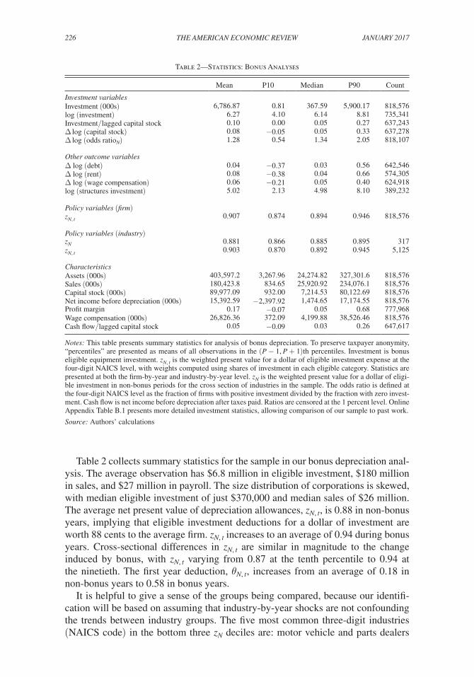


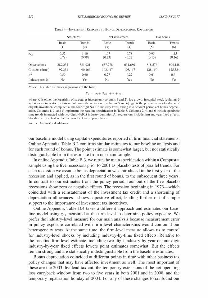


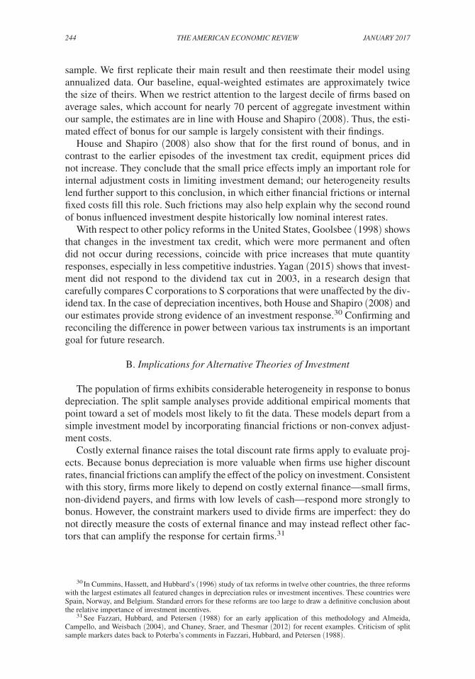


![Zwick 3130 SHORE [E]](https://static.documents.pub/doc/80x56/619f68d33d79844e314e656b/zwick-3130-shore-e.jpg)


