Taxing Retirement Income: Nonqualified Annuities … taxation of retirement saving is an important...

Taxing Retirement Income

563

Abstract - This paper explores the current tax treatment of non-qualified immediate annuities and distributions from tax-qualifiedretirement plans in the United States. First, we describe how im-mediate annuities held outside retirement accounts are taxed. Weconclude that the current income tax treatment of annuities doesnot substantially alter the incentive to purchase an annuity ratherthan a taxable bond. We nevertheless find differences across differ-ent individuals in the effective tax burden on annuity contracts.Second, we examine an alternative method of taxing annuities thatwould avoid changing the fraction of the annuity payment that isincluded in taxable income as the annuitant ages, but would stillraise the same expected present discounted value of revenues as thecurrent income tax rule. We find that a shift to a constant inclu-sion ratio increases the utility of annuitants and that this increaseis greater for more risk averse individuals. Third, we examine howpayouts from qualified accounts are taxed, focusing on both annu-ity payouts and minimum distribution requirements that constrainthe feasible time path of nonannuitized payouts. We describe brieflythe origins and workings of the minimum distribution rules andwe also provide evidence on the fraction of retirement assets poten-tially affected by these rules.

Die early and avoid the fate.Or, if predestined to die late,Make up your mind to die in state.

—Robert Frost in “Provide, Provide”

The taxation of retirement saving is an important andgrowing policy issue. Income tax exclusions for contri-

butions to qualified retirement plans and for the income thataccrues on the assets held in such plans have an importantimpact on the structure of retirement saving for many house-holds. A substantial fraction of those reaching retirement agein recent years have accumulated very few financial assetsoutside retirement saving plans. Moore and Mitchell (forth-coming) and Poterba, Venti, and Wise (1998a) show that So-cial Security wealth, employer-provided pensions, andowner-occupied housing equity were the most substantialcomponents of household net worth for all but the wealthi-est one-fifth of retirees in the 1990s.

Taxing Retirement Income: NonqualifiedAnnuities and Distributions from

Qualified Accounts

National Tax JournalVol. LII, No. 3

Jeffrey R. BrownJohn F. Kennedy Schoolof Government,Harvard University,andNBER, Cambridge,MA 02138

Olivia S. MitchellWharton School,University of Pennsyl-vania, Philadelphia, PA19104

NBER, Cambridge,MA 02138

James M. PoterbaMassachusetts Instituteof Technology andNBER, Cambridge,MA 02139

Mark J. WarshawskyTIAA-CREF Institute,New York, NY 10017

NATIONAL TAX JOURNAL

564

For households that do accumulate sub-stantial assets during their workinglives—both inside and outside qualifiedretirement plans—reaching retirementraises questions about how to draw downthese assets. Someone who has no inter-est in leaving a bequest, and who does notknow how long he will live, faces theproblem of choosing a level of consump-tion that will take advantage of his accu-mulated assets, without incurring toogreat a risk of outliving his resources. Oneway to avoid this risk is to purchase animmediate life annuity contract. Annu-ities, which are sold by life insurance com-panies, typically promise a fixed streamof nominal payouts for as long as the poli-cyholder is alive.

Payouts from retirement assets can bestratified along two dimensions: whetherthe payouts are structured as a life annu-ity and whether the accumulation tookplace in a qualified retirement plan.1 Thistypology gives rise to four types of with-drawals from retirement asset stocks. Thefirst category, income from non-annuitized nonqualified asset accumula-tion, is simply taxable saving. We do notconsider this type of retirement saving inthe present analysis, because it is the sub-ject of essentially all textbook analyses ofhow taxation affects saving behavior. Thesecond category is annuitized payoutsresulting from nonqualified asset accumu-lation. The tax treatment of annuities pur-chased with after-tax dollars is complex.The fraction of annuity payouts that isincluded in the recipient’s taxable incomedepends on how long the annuity hasbeen paying benefits. Annuitants whohave been lucky enough to live a long timeand to receive annuity benefits for a longperiod are taxed on a higher fraction of

their annuity income than are those whohave recently purchased their annuity.This complexity arises from the fact thatpart of each payout on an annuity policyis treated as a return of the policyholder’sprincipal and part is treated as a paymentfrom the capital income that has accruedon the policyholder’s initial premium.

The third payout option consists of an-nuities purchased with assets in qualifiedretirement accounts. The tax treatment inthis case hinges on the presence or absenceof after-tax contributions to the qualifiedaccount. For annuities purchased withfunds in qualified accounts that were par-tially funded with after-tax dollars, the taxtreatment is more complex than for annu-ities purchased from accounts that werefunded only with pretax contributions.

Finally, there is a fourth category ofpayouts: nonannuitized payouts fromqualified retirement plans. These payoutsare subject to a complex set of tax rules, inparticular, minimum distribution require-ments that affect the permissable timepath of nonannuitized distributions.These rules have the potential to affect thetime path along which many elderlyhouseholds draw down their assets.

This paper focuses on two of the fourtypes of withdrawals from retirement sav-ings: annuities purchased using assets thatare held in nonqualified accounts andnonannuitized withdrawals from quali-fied accounts. It is divided into seven sec-tions. The first summarizes the currentfederal income tax rules that apply to non-qualified immediate annuities. Our analy-sis focuses on the payout phase of annuityproducts, and we do not consider the im-portant issues concerning asset accumu-lation that are raised by the rapid recentgrowth of variable annuity products. The

1 The most common type of qualified retirement plan is offered to employees by an employer and meetsInternal Revenue code criteria permitting the plan to accumulate tax-protected assets. The employer’scontributions to such plans are deductible and they are not considered taxable income to the employee. Theinvestment earnings on assets in the account are tax exempt at the time they are earned. IRAs, tax-deferredannuities, and 401(k) and 403(b) plans funded exclusively by employee contributions are also qualified retire-ment plans.


565

second section describes our frameworkfor calculating the expected present dis-counted value of pretax and after-taxpayouts on annuity policies. It also ex-plains how we can apply a standardmodel of consumer behavior to estimatethe utility consequences of various taxrules for annuity products. The third sec-tion presents our basic findings on howthe current income tax system affects theafter-tax value of annuity purchases. Wefind that the current income tax rules donot substantially affect the incentives topurchase annuities rather than taxablebonds. We nevertheless find some differ-ences across categories of individuals inthe effective tax burden on annuity con-tracts.

The fourth section develops an alterna-tive tax scheme for nonqualified annuitiesthat would include a constant fraction ofannuity payouts in taxable income, re-gardless of how long the annuity had beenpaying benefits. We calibrate this taxscheme by finding the inclusion rate atwhich it would raise the same expectedpresent discounted value of revenues asthe current tax system, and we also askhow such a tax system would affect theincentives for annuity purchase.

The fifth section moves beyond the dis-cussion of nonqualified annuity productsto an overview of tax issues that arise inconnection with qualified accounts. First,we consider annuitized payouts fundedwith after-tax contributions. We describethe minimum distribution requirementsassociated with nonannuitized payoutsfrom qualified retirement accounts. Ourdiscussion focuses on how these require-ments constrain the feasible time path ofpayouts. We examine detailed provisionssuch as assumptions about mortalitytables and allowable distribution meth-ods.

The sixth section presents evidence onthe amount of retirement assets and thefraction of retiree households that are po-tentially affected by minimum distribu-

tion rules. We report the value of assets inqualified pension plans that are held byindividuals who are approaching the ageat which minimum distributions mustbegin. The conclusion raises several issuesthat warrant further research attention,and an Appendix presents estimates of therevenue consequences of changing thecurrent minimum distribution rules.

THE CURRENT TAX TREATMENT OFNONQUALIFIED ANNUITIES

The current U.S. federal income tax sys-tem taxes both the income from annuitycontracts and the capital income that apotential annuitant might earn on his al-ternative investment options. Throughoutthis paper, we consider an investment ina taxable bond as the alternative to pur-chasing an annuity contract. The U.S. Gen-eral Accounting Office (1990) provides anintroduction to the tax rules that governnonqualified annuities. First, the InternalRevenue Service (IRS) specifies the timeperiod over which the annuitant can ex-pect to receive benefits. We denote this ex-pected payout period T’. The IRS regula-tions refer to it as the “Expected ReturnMultiple,” and it is currently based on theunisex IRS annuitant mortality table aswell as the annuitant’s age at the timewhen the annuity begins paying benefits.The current tax rules apply the same mor-tality rates, and hence expected payout pe-riods, to annuity payouts received by menand by women, even though the actualmortality rates facing men and women aresubstantially different.

Second, the tax law prescribes an inclu-sion ratio (λ), which determines the shareof each annuity payment that must be in-cluded in the recipient’s taxable income.The inclusion ratio is related to the frac-tion of each annuity payout that resultsfrom capital income on the accumulatingvalue of the annuity premium rather thanfrom a return of the annuitant’s principal.


566

This method of taxing annuity payments,known as the “General Rule,” is requiredfor all nonqualified annuity paymentsstarting after July 1, 1986. A second ap-proach, known as the “SimplifiedMethod,” applies to certain qualified an-nuities purchased after November 19,1996. It specifies different values of theinclusion ratio than the general rule, butotherwise operates in a similar fashion.

For an annuity policy with a purchaseprice of Q and an annual payout of A, theinclusion ratio during the first T’ years ofpayouts is defined by

[1]

After T’ years, all payouts from the an-nuity policy are included in taxable in-come (thus λ = 1 after T’ years).2 If the an-nuitant faces a combined federal and statemarginal income tax rate of τ, then theafter-tax annuity payment in each year is(1 – λτ )A. If an equivalently risky taxablebond yields a pretax nominal return of i,its after-tax return is (1 – τ)i. The expectedreturn multiple, T’, is equal to theannuitant’s life expectancy as of the start-ing date of the annuity, calculated usingthe IRS’s unisex annuitant mortality table.

COMPARING ANNUITIES WITHALTERNATIVE ASSETS

We use two approaches to analyze thecurrent tax treatment of annuities versustaxable bonds. The first emphasizes theexpected present discounted value of af-ter-tax annuity payments and the com-parison between this value and the pur-chase cost of the annuity. The second,which uses an explicit utility function,asks how much wealth a stylized con-

sumer would need if he could not buy anannuity in order to be as well off as if hecould invest his actual current wealth ina nominal annuity contract. We now de-scribe each of these approaches in turn.

The Expected Discounted Present Valueof Annuity Payouts

The expected present discounted value(EPDV) of the payouts from an immedi-ate annuity depends on the amount of theannuity payout (A), the discount rate thatapplies to future annuity payouts, and themortality rates that determine theannuitant’s chances of surviving to receivethe promised future payouts. We denotethe probability of surviving for j monthsafter purchasing the annuity as Pj. We fo-cus on months as the basic time unit be-cause annuities typically pay monthly ben-efits. If there were no taxes, the expectedpresent discounted value of annuitypayouts (EPDVnotax) for someone at age 65,and who was certain to die before age 115(600 months into the future), would be

[2]

where ik denotes the nominal one-periodinterest rate k periods into the future. Ex-pressions such as EPDVnotax have beenused in a number of earlier studies, in-cluding Warshawsky (1988), Friedmanand Warshawsky (1988, 1990), andMitchell, Poterba, Warshawsky, andBrown (hereafter, MPWB) (1999).

In the current income tax environment,this expression must be modified to rec-ognize both the income tax treatment of

λ = 1 – A * T’

.Q

2 Adney, McKeever, and Seymon-Hirsch (1998) discuss the estate tax treatment of annuity contracts wherepayments continue after death. These issues are beyond the scope of this paper. It is worth noting, however,that, according to most interpretations of the current law and regulations, payouts from a deferred annuitycontract must be taxed either as a lump sum payment or, under the General Rule, as a life annuity. This forcesan either/or payout choice on contract holders and thus denies them the possibility of using both payoutoptions in a single contract.

EPDVnotax =A * Pj

600

j=1Σ

Πj

k=1

(1 + ik)


567

annuity payments and the taxation of thereturns on the alternative asset that deter-mines the discount rate for the annuitycash flows. The modified expression in anincome tax world, EPDVtax, is

[3]

with T’ and λ defined as above. The dif-ference between EPDVnotax and EPDVtax

provides a direct measure of the extent towhich the current income tax structureaffects the attractiveness of annuitiesrather than taxable bonds, relative to aworld in which capital income is untaxed.If the two EPDV values are similar, thenthe current income tax code does not sub-stantially affect the incentive to purchaseannuities rather than taxable bonds. It isthe relative tax treatment of annuities andbonds that determines the effective taxburden on annuities.

Data Inputs to EPDV Calculations

We apply this framework to evaluatethe expected discounted value of annuitypayouts for annuity products that wereavailable in the U.S. marketplace in 1998.We focus on individual nonparticipating,single-premium-immediate life annuitiesoffered by commercial life insurance com-panies. These are annuity policies forwhich individuals make an initial pre-mium payment and then usually beginreceiving fixed annuity payouts in themonth after their purchase.

Payments on life annuities (variable Ain equations 2 and 3) are reported eachyear in the August issue of A. M. Best’spublication Best’s Review: Life and Health.We analyze data from the August 1998

issue, which reports the results of an an-nuity market survey conducted at the be-ginning of June 1998. The Best’s data cor-respond to single-premium annuities witha $100,000 premium. Ninety-nine compa-nies responded to the survey, reportinginformation on the current monthlypayouts on individual annuities sold tomen and women at ages 55, 60, 65, 70, 75,and 80. We restrict our current analysis toannuities available for 65-year-old men andwomen. Poterba and Warshawsky (1999)summarize the average annuity payouts atdifferent ages. The computations belowfocus on a hypothetical individual whopurchases an annuity that offers the aver-age payout across all companies. We rec-ognize, and document in MPWB (1999),that there is substantial variation in annu-ity payouts across insurers.

To evaluate the rate of return that po-tential annuitants might receive on alter-native assets, we assume that annuitypayouts are riskless. We then use the termstructure of yields for zero-coupon Trea-sury “strips” to estimate the pattern offuture monthly short-term interest rates.These data are published in the Wall StreetJournal, and we use the reports from thefirst week of June 1998 to coincide withthe timing of Best’s annuity price survey.

Our EPDV calculations are sensitive toour marginal tax rate assumptions. Be-cause there is very little publicly availableinformation on the household incomes,and even less on the marginal tax rates, ofannuity purchasers, we consider two dif-ferent marginal tax rate assumptions. Inthe first case, we assume that the annuitybuyer faces a 15 percent federal marginaltax rate; and in the second case, the annu-ity recipient is assumed to be in the 36 per-cent federal tax bracket. The first case, cor-responds to a married couple filing jointlywith total taxable income of less than$42,350, while the second would corre-spond, in 1998, to taxable income between$155,950 and $278,450. We also reportEPDV calculations for the no-tax case.

(1 + (1 – τ) * ik)+ Σ j

(1 – τ) * A * Pj600

j =12*T’+ 1 Πk = 1

EPDVtax = Σ j

(1 – λ * τ) * A * Pj12*T’

j=1(1 + (1 – τ) * ik)Π

k=1


568

We evaluate equations 2 and 3 usingprojected survival probabilities for peoplepurchasing annuities in 1998. One diffi-culty in evaluating the effective cost ofpurchasing an annuity, however, is thatthe pool of actual annuity purchasers hasa lower risk of dying at any given age thanthe population at large. Insurance compa-nies use an annuitant mortality table todetermine the relationship between pre-mium income and the expected presentdiscounted value of payouts. We use theMPWB (1999) approach to projecting fu-ture annuitant mortality rates by combin-ing information from the Annuity 2000Mortality table, the older 1983 IndividualAnnuitant Mortality (IAM) table, and theprojected rate of mortality improvementin the Social Security Administration’spopulation mortality tables from the 1995Social Security Trustee’s Report.

The choice of a mortality table is a keyissue in the taxation of annuity payouts.In this respect, the current IRS use of the1983 IAM table has important conse-quences. The 1983 IAM table was basedon actual annuitants’ mortality experiencein a large group of companies over the pe-riod 1971–6, updated to reflect 1983 con-ditions. The Society of Actuaries’ Indi-vidual Annuity Experience Committee(1991–2) studied the annuity experienceof a small group of companies over theperiod 1976–86 and concluded that the1983 table was adequate for the 1980s.

More recently, however, Johansen(1996)—one of the actuaries involved inthe earlier studies—has called for a newindividual annuity table, after evaluatingpopulation mortality statistics from theSocial Security Administration and theNational Center for Health Statistics andevolving conditions in the group annuitymarket. Unfortunately, there are no recentstudies of industry-wide annuitant mor-tality experience. A Society of Actuariescommittee therefore suggested using thebasic 1983 annuity table projected forwardto the year 2000, with mortality improve-ment factors consistent with the recentexperience of the general population aswell as that of one company with substan-tial annuity business. This is the Annuity2000 table. We construct a 1998 annuitantmortality table by interpolating betweenthe 1983 IAM and the Annuity 2000 tablesand then applying forward looking mor-tality improvement factors to create a 1998annuitant cohort table. The age and gen-der-specific mortality rates in the 1998table are substantially lower than those inthe 1983 IAM table due to significant mor-tality improvements.

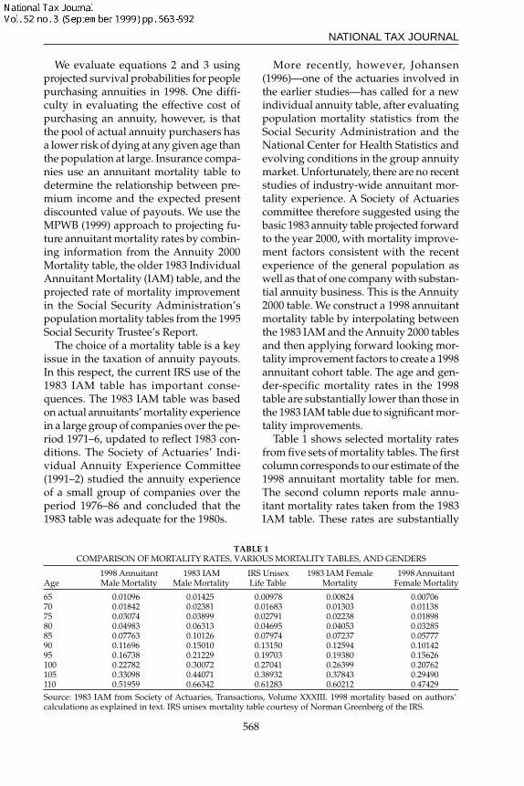
Table 1 shows selected mortality ratesfrom five sets of mortality tables. The firstcolumn corresponds to our estimate of the1998 annuitant mortality table for men.The second column reports male annu-itant mortality rates taken from the 1983IAM table. These rates are substantially

TABLE 1COMPARISON OF MORTALITY RATES, VARIOUS MORTALITY TABLES, AND GENDERS

65707580859095100105110

0.01096 0.01842 0.03074 0.04983 0.07763 0.11696 0.16738 0.22782 0.33098 0.51959

0.01425 0.02381 0.03899 0.06313 0.10126 0.15010 0.21229 0.30072 0.44071 0.66342

0.00978 0.01683 0.02791 0.04695 0.07974 0.13150 0.19703 0.27041 0.38932 0.61283

0.00824 0.01303 0.02238 0.04053 0.07237 0.12594 0.19380 0.26399 0.37843 0.60212

0.00706 0.01138 0.01898 0.03285 0.05777 0.10142 0.15626 0.20762 0.29490 0.47429

Source: 1983 IAM from Society of Actuaries, Transactions, Volume XXXIII. 1998 mortality based on authors’calculations as explained in text. IRS unisex mortality table courtesy of Norman Greenberg of the IRS.

Age1998 AnnuitantMale Mortality

1983 IAMMale Mortality

IRS UnisexLife Table

1983 IAM FemaleMortality

1998 AnnuitantFemale Mortality


569

greater than those in the 1998 annuitanttable. For most ages, the mortality rate formen according to the 1983 IAM table isapproximately 30 percent higher than themortality rate in the 1998 annuitant table.The third column shows the 1983 UnisexIndividual Annuitant Mortality table,which is what the IRS currently uses todetermine the inclusion ratio and other taxparameters associated with annuity taxa-tion. The last two columns show the 1998and 1983 annuitant mortality rates forwomen.

The 1983 Unisex Mortality table that theIRS uses is a weighted average of the 1983IAM basic mortality tables for men andwomen, with different weights on the twotables at different ages. We have “reverseengineered” these weights and havefound them to vary with age and to placeheavier emphasis on female than malemortality. For example, at age 65, theUnisex table places a weight of 0.74 on thefemale mortality rate and 0.26 on the malerate. This weight on the female mortalityrates decreases to 0.65 at age 70 and thenincreases every five years until it peaks at0.825 for age 95 and above. We have beenunable to learn the motivation for thisparticular choice of weights. The U.S.Treasury Department has recently revisedthe mortality tables that are used to valuethe benefits of group life insurance andseveral other insurance products, butthere have been no changes since 1986 inthe mortality table that is used to computeT’ in single-premium annuity markets.

For men, the fact that the IRS UnisexMortality table overstates mortality ratesby using an old mortality table is almostexactly offset by the heavier weighting onthe lower female mortality rates. There-fore, the IRS Unisex table does notsubstantially differ from the 1998 male an-nuitant mortality table. For women, how-ever, the differences between the twotables are large. Both the weightingscheme and the outdated table result inIRS mortality rates for women that are

substantially larger than the mortalityrates from the 1998 annuitant table. Thesedifferences are especially large at theyounger ages. At age 65, for example, awoman’s mortality rate is 40 percentgreater in the IRS table than in the 1998annuitant table.

The use of a unisex mortality table im-plies that there are differences in the ef-fective tax burdens on annuities for menand women. According to the IRS unisextable, the life expectancy of a 65-year-oldindividual is 20 years. This is the valueused for T’ in the construction of the in-clusion ratio. The actual life expectancyof a 65-year-old man, according to the 1998annuitant table, is 19.8 years, while thatfor a 65-year-old woman is 22.7 years.

The fact that T’ for women is less thantheir actual life expectancy has two effectson the lifetime tax burden on annuities.First, using the IRS table results in asmaller inclusion ratio (λ) than a womanwould face if her actual life expectancywere used. In the early years of an annu-ity payout, a lower inclusion ratio impliesthat a smaller fraction of the annuity pay-ment is subject to taxation. This effecttherefore reduces the tax burden on an-nuities.

For example, in 1998, a 65-year-oldwoman purchasing the average single-premium-immediate annuity offered inthe private market could expect to receiveapproximately $662 per month for a$100,000 policy. Under current IRS rules,the value of T’ is 20 years, which impliesan inclusion ratio (λ) for this woman of0.37. This means that $245 of the $662 an-nuity payment is included in taxable in-come, while the remainder is considereda return of basis and is tax free. If insteadof using the 20-year life expectancy im-plied by the 1983 unisex table, the IRSused the 1998 female annuitant mortalitytable, this would increase the value of T’to be equal to her actual life expectancyof 22.7 years. This in turn raises the inclu-sion ratio to λ = 0.445, which would re-


570

sult in $295 of the $662 monthly annuitypayment being included in taxable in-come. Therefore, by using the 20-year lifeexpectancy of the 1983 unisex mortalitytable instead of the life expectancy fromthe 1998 female annuitant table, the65- year-old female annuitant’s taxable in-come is reduced by $50 per month, or $600per year.

The second effect of using a lower valueof T, and one that offsets the first effect toa small degree, is the fact that using theIRS unisex table also reduces the numberof years for which part of the annuity pay-ment is excluded from taxes. Under cur-rent law, after 20 years (when the womanreaches age 85), the after-tax annuity pay-ment falls from (1 – λτ )A to (1 – τ)A. (Taxesrise from λτA to τA.) Using actual life ex-pectancy, this drop would occur after 22.7years. Therefore, the woman would nothave to report the full $662 as taxable in-come until she was age 87.7.

The net effect of using the 1983 unisextable rather than the current annuitantmortality table is a positive effect on theEPDV of annuity purchase for women.Specifically, a 65-year-old woman with amarginal income tax rate of 28 percentwould have an after-tax EPDV of 0.968using T = 20 from the 1983 Unisex table,versus 0.956 using T = 22.7 from the 1998female annuitant table. The first effect dis-cussed above, the lower inclusion ratiowhen part of the annuity income can beexcluded from taxable income, is quanti-tatively more important than the secondeffect, the change in the length of the timeperiod over which some annuity incomecan be excluded.

A Utility-Based Approach to ValuingAnnuity Products

In addition to our analysis of the ex-pected present discounted value of annu-ity payouts, we also compare annuitiesand alternative assets in terms of the ex-pected utility that they would generate for

a potential annuitant. Because annuitiesoffer individuals insurance against therisk of outliving their assets, they gener-ate benefits that are not captured in asimple present discounted value frame-work. Calculating the expected utility ofannuitization recognizes these benefits,and it provides an explicit framework forevaluating the welfare effects of age-de-pendent taxation of annuity payouts.

Our analysis assumes that a hypotheti-cal individual compares investing in ariskless taxable bond and investing in anactuarially fair annuity contract. This is dif-ferent than our approach in analyzing theEPDV of annuity products, where we usethe actual annuity payouts available in themarketplace rather than hypothetical ac-tuarially fair annuities. We find the actu-arially fair payout per premium dollar, Af,for a 65 year old by solving the equation

[4]

This expression assumes that the insur-ance company providing the annuity isnot taxed, because it uses the pretaxriskless rate of return to discount annuitypayouts. Allowing for insurance companytaxes and other administrative costs ofproviding annuities would reduce the ac-tuarially fair payout, while allowing thehypothetical insurance company to holdriskier, higher return assets would in-crease the actuarially fair payout.

We consider an individual who pur-chases a fixed nominal annuity at age 65.To simplify our calculations, we now as-sume that the annuity pays annual ben-efits. The individual will receive an annu-ity payment in each year that he remainsalive, and his optimal consumption pathwill be related to this payout. The after-tax annuity payout that the individualreceives at age a (Aa) depends on hiswealth at the beginning of retirement

1 = j

Af * Pj600

j = 1Σ

Πk=1

(1 + ik)


571

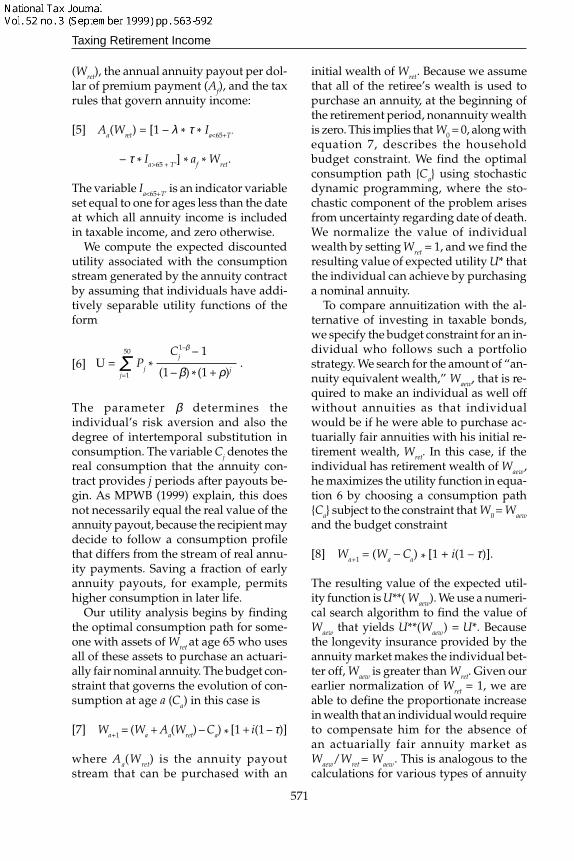
(Wret), the annual annuity payout per dol-lar of premium payment (Af), and the taxrules that govern annuity income:

[5] Aa(Wret) = [1 – λ * τ * Ia<65+T’

– τ * Ia>65 + T’] * af * Wret.

The variable Ia<65+T’ is an indicator variableset equal to one for ages less than the dateat which all annuity income is includedin taxable income, and zero otherwise.

We compute the expected discountedutility associated with the consumptionstream generated by the annuity contractby assuming that individuals have addi-tively separable utility functions of theform

[6]

The parameter β determines theindividual’s risk aversion and also thedegree of intertemporal substitution inconsumption. The variable Cj denotes thereal consumption that the annuity con-tract provides j periods after payouts be-gin. As MPWB (1999) explain, this doesnot necessarily equal the real value of theannuity payout, because the recipient maydecide to follow a consumption profilethat differs from the stream of real annu-ity payments. Saving a fraction of earlyannuity payouts, for example, permitshigher consumption in later life.

Our utility analysis begins by findingthe optimal consumption path for some-one with assets of Wret at age 65 who usesall of these assets to purchase an actuari-ally fair nominal annuity. The budget con-straint that governs the evolution of con-sumption at age a (Ca) in this case is

[7] Wa+1 = (Wa + Aa(Wret) – Ca) * [1 + i(1 – τ)]

where Aa(Wret) is the annuity payoutstream that can be purchased with an

initial wealth of Wret. Because we assumethat all of the retiree’s wealth is used topurchase an annuity, at the beginning ofthe retirement period, nonannuity wealthis zero. This implies that W0 = 0, along withequation 7, describes the householdbudget constraint. We find the optimalconsumption path {Ca} using stochasticdynamic programming, where the sto-chastic component of the problem arisesfrom uncertainty regarding date of death.We normalize the value of individualwealth by setting Wret = 1, and we find theresulting value of expected utility U* thatthe individual can achieve by purchasinga nominal annuity.

To compare annuitization with the al-ternative of investing in taxable bonds,we specify the budget constraint for an in-dividual who follows such a portfoliostrategy. We search for the amount of “an-nuity equivalent wealth,” Waew, that is re-quired to make an individual as well offwithout annuities as that individualwould be if he were able to purchase ac-tuarially fair annuities with his initial re-tirement wealth, Wret. In this case, if theindividual has retirement wealth of Waew,he maximizes the utility function in equa-tion 6 by choosing a consumption path{Ca} subject to the constraint that W0 = Waew

and the budget constraint

[8] Wa+1 = (Wa – Ca) * [1 + i(1 – τ)].

The resulting value of the expected util-ity function is U**( Waew). We use a numeri-cal search algorithm to find the value ofWaew that yields U**(Waew) = U*. Becausethe longevity insurance provided by theannuity market makes the individual bet-ter off, Waew is greater than Wret. Given ourearlier normalization of Wret = 1, we areable to define the proportionate increasein wealth that an individual would requireto compensate him for the absence ofan actuarially fair annuity market asWaew/Wret = Waew. This is analogous to thecalculations for various types of annuity

U = Pj *50 Cj – 11–β

(1 – β) * (1 + ρ)jΣj=1

.


572

products that we report in Brown,Mitchell, and Poterba (1999).

We compute annuity-equivalent wealthin both the current income tax environ-ment and in a case with no taxes, i.e., τ = 0in equations 5, 7, and 8. The difference be-tween the annuity-equivalent wealth cal-culations in the cases with and withoutincome taxation provides information onthe incentive effects of the current incometax treatment of annuities.

TAXATION AND THE VALUATION OFANNUITIES

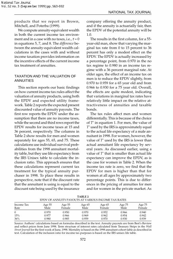
This section reports our basic findingson how current income tax rules affect thevaluation of annuity products, using boththe EPDV and expected utility frame-work. Table 2 reports the expected presentdiscounted value of annuity payouts. Thefirst row reports the EPDV under the as-sumption that there are no income taxes,while the second and third rows report theEPDV results for income taxes at 15 and36 percent, respectively. The columns inTable 2 show results for men and womenseparately for ages 55, 65, and 75. Thesecalculations use individual survival prob-abilities from the 1998 annuitant mortal-ity table, but they use life expectancy fromthe IRS Unisex table to calculate the in-clusion ratio. This approach ensures thatthese calculations represent current taxtreatment for the typical annuity pur-chaser in 1998. To place these results inperspective, note that if the discount ratethat the annuitant is using is equal to thediscount rate being used by the insurance

company offering the annuity product,and if the annuity is actuarially fair, thenthe EPDV of the potential annuity will be1.0.

The results in the first column, for a 55-year-old man, show that varying the mar-ginal tax rate from 0 to 15 percent to 36percent has only a modest effect on theEPDV. The EPDV is actually increased bya percentage point, from 0.970 in the notax regime to 0.980 in an income tax re-gime with a 36 percent marginal rate. Atolder ages, the effect of an income tax onmen is to reduce the EPDV slightly, from0.970 to 0.959 for a 65 year old and from0.966 to 0.930 for a 75 year old. Overall,the effects are quite modest, indicatingthat variations in marginal tax rates haverelatively little impact on the relative at-tractiveness of annuities and taxablebonds.

The tax rules affect men and womendifferentially. This is because of the choiceof T’ in equation 1. For men, the value ofT’ used by the IRS is approximately equalto the actual life expectancy of a male an-nuitant in 1998. For women, however, thevalue of T’ used by the IRS is lower thanactual annuitant life expectancy by sev-eral years. As discussed earlier, using avalue of T’ that is smaller than actual lifeexpectancy can improve the EPDV, as isthe case for women in Table 2. When theincome tax rate is zero, we find that theEPDV for men is higher than that forwomen at all ages by approximately twopercentage points. This is due to differ-ences in the pricing of annuities for menand for women in the private market. As

TABLE 2EPDV OF ANNUITY PAYOUTS AT VARIOUS INCOME TAX RATES

Income TaxRate

015%36%

Age 55Male

0.9700.9770.980

Age 55Female

0.9500.9660.985

Age 65Male

0.9700.9690.959

Age 65Female

0.9520.9620.970

Age 75Male

0.9660.9540.930

Age 75Female

0.9400.9420.939

Source: Authors’ calculations based on formulas described in the text. Annuity payouts are from Best’s Reviewand reflect prices from June 1998. Term structure of interest rates calculated from Treasury Strips in the WallStreet Journal for the first week of June, 1998. Mortality is based on the 1998 annuitant cohort table as described intext. Calculation of the inclusion ratio for income tax purposes is based on the IRS unisex life table.


573

the marginal income tax rate rises, we findthat the EPDV rises more quickly forwomen than for men. In fact, for an in-come tax rate of 36 percent, the EPDV forwomen is actually higher than that formen at any age.

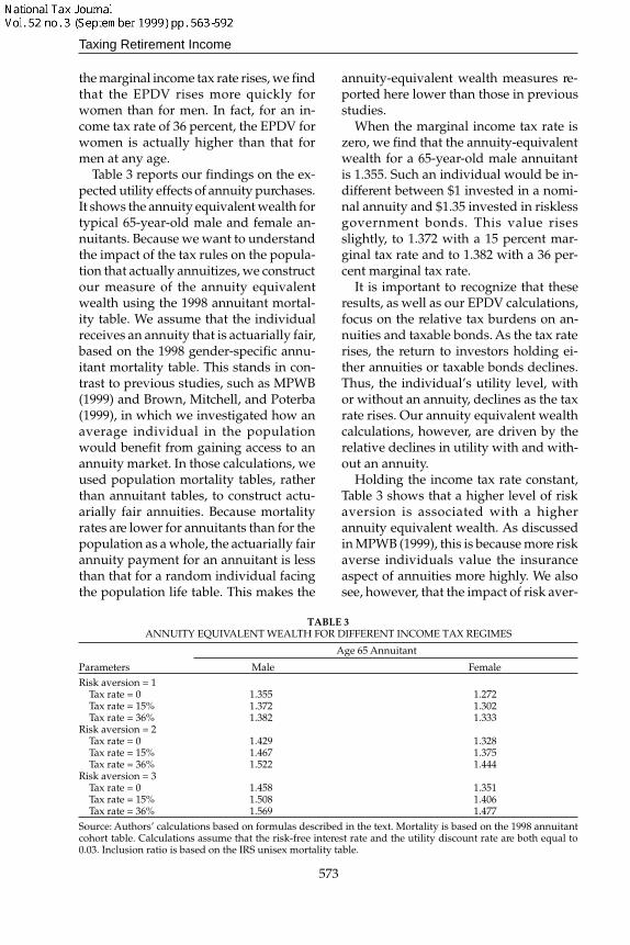
Table 3 reports our findings on the ex-pected utility effects of annuity purchases.It shows the annuity equivalent wealth fortypical 65-year-old male and female an-nuitants. Because we want to understandthe impact of the tax rules on the popula-tion that actually annuitizes, we constructour measure of the annuity equivalentwealth using the 1998 annuitant mortal-ity table. We assume that the individualreceives an annuity that is actuarially fair,based on the 1998 gender-specific annu-itant mortality table. This stands in con-trast to previous studies, such as MPWB(1999) and Brown, Mitchell, and Poterba(1999), in which we investigated how anaverage individual in the populationwould benefit from gaining access to anannuity market. In those calculations, weused population mortality tables, ratherthan annuitant tables, to construct actu-arially fair annuities. Because mortalityrates are lower for annuitants than for thepopulation as a whole, the actuarially fairannuity payment for an annuitant is lessthan that for a random individual facingthe population life table. This makes the

annuity-equivalent wealth measures re-ported here lower than those in previousstudies.

When the marginal income tax rate iszero, we find that the annuity-equivalentwealth for a 65-year-old male annuitantis 1.355. Such an individual would be in-different between $1 invested in a nomi-nal annuity and $1.35 invested in risklessgovernment bonds. This value risesslightly, to 1.372 with a 15 percent mar-ginal tax rate and to 1.382 with a 36 per-cent marginal tax rate.

It is important to recognize that theseresults, as well as our EPDV calculations,focus on the relative tax burdens on an-nuities and taxable bonds. As the tax raterises, the return to investors holding ei-ther annuities or taxable bonds declines.Thus, the individual’s utility level, withor without an annuity, declines as the taxrate rises. Our annuity equivalent wealthcalculations, however, are driven by therelative declines in utility with and with-out an annuity.

Holding the income tax rate constant,Table 3 shows that a higher level of riskaversion is associated with a higherannuity equivalent wealth. As discussedin MPWB (1999), this is because more riskaverse individuals value the insuranceaspect of annuities more highly. We alsosee, however, that the impact of risk aver-

TABLE 3ANNUITY EQUIVALENT WEALTH FOR DIFFERENT INCOME TAX REGIMES

Risk aversion = 1Tax rate = 0Tax rate = 15%Tax rate = 36%



1.3551.3721.382

1.4291.4671.522

1.4581.5081.569

1.2721.3021.333

1.3281.3751.444

1.3511.4061.477

Parameters

Age 65 Annuitant

Male Female

Source: Authors’ calculations based on formulas described in the text. Mortality is based on the 1998 annuitantcohort table. Calculations assume that the risk-free interest rate and the utility discount rate are both equal to0.03. Inclusion ratio is based on the IRS unisex mortality table.


574

sion is greater in a high income tax regime.For example, increasing risk aversionfrom 1 to 3 increases the annuity equiva-lent wealth from 1.355 to 1.458 when themarginal tax rate is zero, an increase of0.103, while with a 36 percent marginaltax rate, the annuity-equivalent wealthrises from 1.382 to 1.569, an increase of0.187.

The second column of Table 3 reportsthe same results for a 65-year-old woman.Overall, a female annuitant’s annuityequivalent wealth for an actuarially fairannuity is lower than for a man. This dif-ference arises due to women experienc-ing lower mortality rates than men. Therate of return on an annuity can be viewedas being the sum of the risk-free interestrate, r, plus a mortality premium that isan increasing function of an individual’smortality rate q. For an infinitely lived in-dividual, the mortality premium is zero,and an annuity is identical to a risklessbond. For a person facing a constant prob-ability q of dying each period, the grossreturn on an actuarially fair annuity is(1 + r)/(1 – q) each period. For small val-ues of r and q, the net return is approxi-mately equal to r + q/(1 – q). The secondterm reflects the probability that otherannuity buyers in the individual’s annu-ity cohort die during the period, scaled upby a 1/(1 – q) factor that reflects the divi-sion of the principal of those annuitantswho die among the fraction, 1 – q, whoremain alive. Because mortality is higherfor men than women, their mortality pre-mium, q/(1 – q), is also higher.

Men find actuarially fair annuities moreattractive than women do, provided thatannuities are priced in this gender-specificmanner. While the annuity equivalentwealth differs, we find that the effect ofdifferent tax regimes is quite similar formen and women. Specifically, the annu-ity equivalent wealth rises with the mar-ginal income tax rate, and this differenceis rising with risk aversion for bothgroups.

Our numerical analysis focuses on therelative tax burden on annuities and tax-able bonds, but it does not consider thequestion of how annuities would be taxedin an ideal income tax setting. This is adifficult question, and one for which ourdecomposition of the annuity return intointerest on the invested principal and apayout based on the invested principal ofthose annuitants who have already diedproves helpful. The fixed nominal annu-ity payouts offered by the annuity con-tracts we consider in fact combine thesetwo sources of return with a partial returnof principal in each period. In general, therelative importance of each of these com-ponents will vary over the annuity’s life-time. Right after the annuitant purchaseshis annuity, a relatively large fraction ofthe annuity payout will represent a returnon principal, while a relatively small sharewill represent a return of principal. (It maybe helpful in this context to think of a levelpayment, self-amortizing mortgage, inwhich the fraction of each mortgage pay-ment that represents a repayment of prin-cipal rises over the life of the contract.)This consideration alone would suggestthat the share of each annuity payouttreated as taxable income would rise overtime under an ideal income tax.

However, there is another potentiallyoffsetting effect, due to variation over timein the share of the annuity payouts, whichis due to mortality within the annuitypool. Because mortality rates rise with age,the mortality premium q/(1 – q) describedabove is also increasing with age. Becausemost annuity contracts provide a fixednominal stream of payments, however,this mortality premium is smoothed overthe potential life of the annuitant. Thiscomplicates the decomposition of the an-nuity payment into its component parts.

Furthermore, it is not clear how suchpayouts should be taxed under an idealincome tax. If they were taxed in the sameway as other insurance products, such aslife insurance, they would be excluded


575

from the tax base. Life insurance is cur-rently purchased with after-tax dollars,and the payouts from life insurance poli-cies are usually untaxed. If the return ofprincipal invested by other annuitants istreated instead as a lottery winning, itwould be included in the income tax base.Recognizing this important and poten-tially time-varying source of annuitypayouts, and its ambiguous tax treatment,makes it difficult to make any simple yetgeneral statement regarding the fractionof annuity payouts that would be taxedunder an ideal income tax.

ALTERNATIVES TO THE CURRENTAPPROACH TO TAXING ANNUITIES

The use of a time-varying inclusion ra-tio, with a single step change when theannuitant has received benefits for theexpected return multiple (T’), is a key fea-ture of the current income tax treatmentof annuity payouts. This tax provision hasthe effect of raising the tax burden andreducing the after-tax income from anannuity for those individuals who havereceived the largest total payouts fromtheir annuity contracts. A difficulty withthis approach is that it results in a signifi-cant drop in the level of benefits at a dis-crete point in time, after which the after-tax benefit stays at this lower level for theduration of the annuitant’s life.

For example, a 65-year-old woman pur-chasing an average priced annuity in 1998will, under current tax rules, face an inclu-sion ratio (λ) of approximately 0.43. If shefaces a 36 percent marginal tax rate (τ), thismeans that at the start of her annuity con-tract, for every $1 of nominal annuity in-come received on a before-tax basis, she willbe able to consume (1 – λτ) dollars, or $0.845.Twenty years after the annuity payouts be-gin, at age 85, her tax rate on annuity in-come rises from λτ = 15.5 percent to τ = 36percent. This reduces her after-tax con-sumption stream to $0.64. This discontinu-ous drop in the after-tax nominal annuity

exacerbates the decline in the real value ofa fixed nominal annuity that occurs as a re-sult of inflation. If the inflation rate is a fixed3 percent per year, over a 20-year period,the real value of the annuity income de-clines to 55 percent of its initial value on abefore-tax basis. Combining this with theincrease in the inclusion ratio means thatthe after-tax, real income available for con-sumption at age 85 is only $0.354 per dollarof real annuity income at the beginning ofthe annuity contract. This represents nearlya 60 percent decline in the after-tax realvalue of the annuity over a 20-year period.

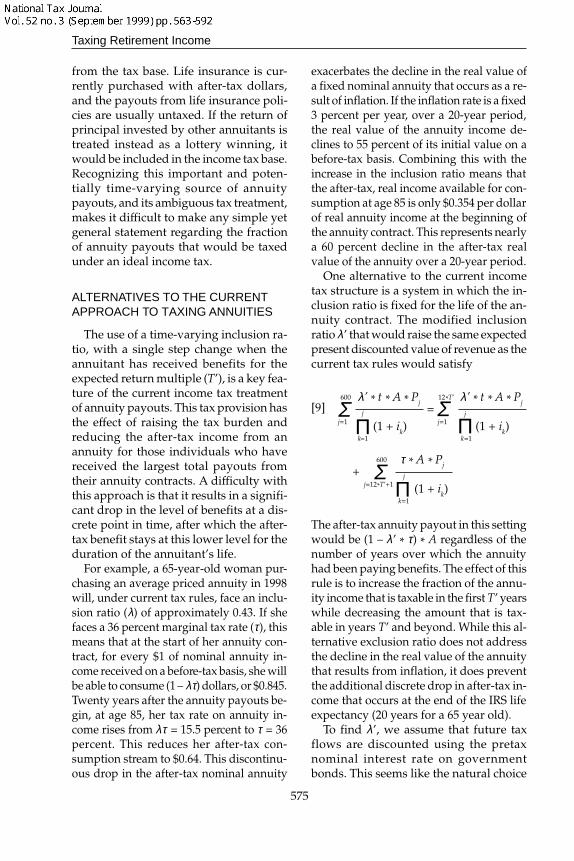
One alternative to the current incometax structure is a system in which the in-clusion ratio is fixed for the life of the an-nuity contract. The modified inclusionratio λ’ that would raise the same expectedpresent discounted value of revenue as thecurrent tax rules would satisfy

[9]

The after-tax annuity payout in this settingwould be (1 – λ’ * τ) * A regardless of thenumber of years over which the annuityhad been paying benefits. The effect of thisrule is to increase the fraction of the annu-ity income that is taxable in the first T’ yearswhile decreasing the amount that is tax-able in years T’ and beyond. While this al-ternative exclusion ratio does not addressthe decline in the real value of the annuitythat results from inflation, it does preventthe additional discrete drop in after-tax in-come that occurs at the end of the IRS lifeexpectancy (20 years for a 65 year old).

To find λ’, we assume that future taxflows are discounted using the pretaxnominal interest rate on governmentbonds. This seems like the natural choice

λ’ * t * A * Pj600

=j=1

j

k=1

ΣΠ (1 + ik)

λ’ * t * A * Pj12*T’

j=1j

k=1

ΣΠ (1 + ik)

600 τ * A * Pj

j=12*T’+1j

k=1

ΣΠ (1 + ik)

+


576

when the federal government is the dis-counting agent. We can repeat both theEPDV and equivalent wealth gain calcu-lations using this modified income taxrule. While we have held the expected dis-counted value of revenue constant acrossregimes with different inclusion ratios, therevenue is discounted at the before-taxrather than the after-tax Treasury rate. Thismeans that there can be differences in theEPDV of after-tax annuity payouts in thedifferent inclusion ratio regimes, becausethe EPDV calculation is done from theperspective of the individual annuitantusing after-tax interest rates.

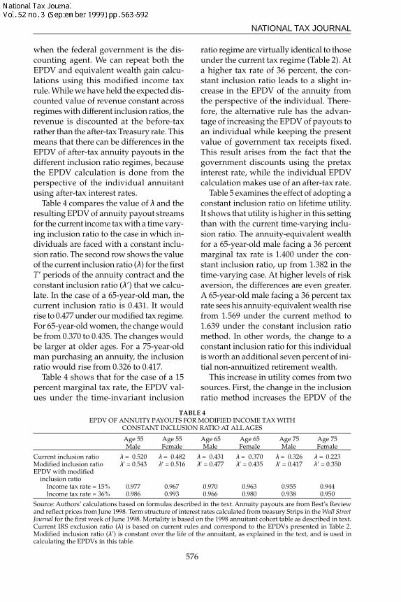
Table 4 compares the value of λ and theresulting EPDV of annuity payout streamsfor the current income tax with a time vary-ing inclusion ratio to the case in which in-dividuals are faced with a constant inclu-sion ratio. The second row shows the valueof the current inclusion ratio (λ) for the firstT’ periods of the annuity contract and theconstant inclusion ratio (λ’) that we calcu-late. In the case of a 65-year-old man, thecurrent inclusion ratio is 0.431. It wouldrise to 0.477 under our modified tax regime.For 65-year-old women, the change wouldbe from 0.370 to 0.435. The changes wouldbe larger at older ages. For a 75-year-oldman purchasing an annuity, the inclusionratio would rise from 0.326 to 0.417.

Table 4 shows that for the case of a 15percent marginal tax rate, the EPDV val-ues under the time-invariant inclusion

ratio regime are virtually identical to thoseunder the current tax regime (Table 2). Ata higher tax rate of 36 percent, the con-stant inclusion ratio leads to a slight in-crease in the EPDV of the annuity fromthe perspective of the individual. There-fore, the alternative rule has the advan-tage of increasing the EPDV of payouts toan individual while keeping the presentvalue of government tax receipts fixed.This result arises from the fact that thegovernment discounts using the pretaxinterest rate, while the individual EPDVcalculation makes use of an after-tax rate.

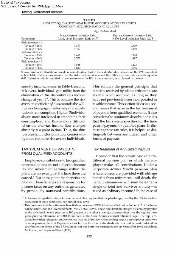
Table 5 examines the effect of adopting aconstant inclusion ratio on lifetime utility.It shows that utility is higher in this settingthan with the current time-varying inclu-sion ratio. The annuity-equivalent wealthfor a 65-year-old male facing a 36 percentmarginal tax rate is 1.400 under the con-stant inclusion ratio, up from 1.382 in thetime-varying case. At higher levels of riskaversion, the differences are even greater.A 65-year-old male facing a 36 percent taxrate sees his annuity-equivalent wealth risefrom 1.569 under the current method to1.639 under the constant inclusion ratiomethod. In other words, the change to aconstant inclusion ratio for this individualis worth an additional seven percent of ini-tial non-annuitized retirement wealth.

This increase in utility comes from twosources. First, the change in the inclusionratio method increases the EPDV of the

TABLE 4EPDV OF ANNUITY PAYOUTS FOR MODIFIED INCOME TAX WITH

CONSTANT INCLUSION RATIO AT ALL AGES

Current inclusion ratioModified inclusion ratioEPDV with modified

inclusion ratioIncome tax rate = 15%Income tax rate = 36%

Age 55Male

λ = 0.520λ’ = 0.543

0.9770.986

Age 55Female

λ = 0.482λ’ = 0.516

0.9670.993

Age 65Male

λ = 0.431λ’ = 0.477

0.9700.966

Age 65Female

λ = 0.370λ’ = 0.435

0.9630.980

Age 75Male

λ = 0.326λ’ = 0.417

0.9550.938

Age 75Female

λ = 0.223λ’ = 0.350

0.9440.950

Source: Authors’ calculations based on formulas described in the text. Annuity payouts are from Best’s Reviewand reflect prices from June 1998. Term structure of interest rates calculated from treasury Strips in the Wall StreetJournal for the first week of June 1998. Mortality is based on the 1998 annuitant cohort table as described in text.Current IRS exclusion ratio (λ) is based on current rules and correspond to the EPDVs presented in Table 2.Modified inclusion ratio (λ’) is constant over the life of the annuitant, as explained in the text, and is used incalculating the EPDVs in this table.


577

annuity income, as seen in Table 4. Second,risk averse individuals gain utility from theelimination of the discontinuous incomechange at year T’. This is because the riskaversion coefficient β also controls the will-ingness to engage in intertemporal substi-tution in consumption. Higher β individu-als are more interested in smoothing theirconsumption, and this is more difficultwhen the after-tax income flow changesabruptly at a point in time. Thus, the shiftto a constant inclusion ratio increases util-ity more for more risk averse individuals.

TAX TREATMENT OF PAYOUTSFROM QUALIFIED ACCOUNTS

Employee contributions to tax-qualifiedretirement plans are not subject to incometax and investment earnings within theplans are tax exempt at the time these areearned.3 But at the point that benefits arepaid out, beneficiaries are responsible forincome taxes on any outflows generatedby previously nontaxed contributions.

This follows the general principle thatbenefits received by plan participants aretaxable when received, as long as theyhave not previously been incorporated intaxable income. This section discusses sev-eral issues that arise in the tax treatmentof payouts from qualified accounts. It alsoconsiders the minimum distribution rulesthat the tax system specifies for the timepath of payouts for qualified plans. In dis-cussing these tax rules, it is helpful to dis-tinguish between annuitized and otherforms of payouts.

Tax Treatment of Annuitized Payouts

Consider first the simple case of a tra-ditional pension plan in which the em-ployer makes all contributions. Under acorporate defined benefit pension planwhere retirees are provided with old-agebenefits from retirement until death, thebenefit stream—which may be either asingle or joint and survivor annuity—istaxed as ordinary income.4 In the case of

TABLE 5ANNUITY EQUIVALENT WEALTH FOR MODIFIED INCOME TAX WITH

CONSTANT INCLUSION RATIO AT ALL AGES

Risk aversion = 1Tax rate = 15%Tax rate = 36%



1.3771.400

1.4811.573

1.5281.639

1.3091.358

1.3901.497

1.4231.546

Parameters

Age 65 Annuitant

Male, Current Inclusion Ratio0.431, Level Inclusion Ratio 0.477

Female, Current Inclusion Ratio0.370, Level Inclusion Ratio 0.435

Source: Authors’ calculations based on formulas described in the text. Mortality is based on the 1998 annuitantcohort table. Calculations assume that the risk-free interest rate and the utility discount rate are both equal to0.03. Inclusion ratio is modified to be constant over the life of the annuitant, as explained in the text.

3 Achieving tax-qualified status for a retirement plan requires that the plan be approved by the IRS; for furtherdiscussion of these conditions, see McGill et al. (1996).

4 This presumes that the retirement benefit does not exceed ERISA limits spelled out in Section 415 of the Inter-nal Revenue Code and its amendments (McGill et al., 1996). These rules limit the straight life annuity payableunder a defined benefit pension to 100 percent of a worker’s average compensation over the highest threeyears prior to retirement, or $90,000 (indexed) at the Social Security normal retirement age. The cap is re-duced for earlier retirement and/or for less than ten of service. Other ceilings apply if an employer offers twoor more pension plans. A 15 percent excise tax was levied on individuals who received defined contributiondistributions in excess of the ERISA limits, but this limit was suspended for tax years after 1997; see Adney,McKeever, and Seymon-Hirsch (1998).


578

a company-sponsored defined contributionpension, the taxation of payouts is alsosimple when the employer has directlyfinanced the entire contribution or whenthe plan participant pays into the pensionusing only pretax income, as is commonunder 401(k) pension plans. In these situ-ations, retirement benefit streams areagain fully taxable at the recipient’s mar-ginal tax rate.

The taxation of qualified plans becomesmore complicated when employees arerequired to contribute to their qualifiedretirement accounts using after-tax in-come. In the private defined benefit arena,this is uncommon, but the practice iswidespread among state and local pen-sions. Mitchell and McCarthy (1999) findthat almost three-quarters of all full-timepublic sector plan participants are re-quired to contribute to their defined ben-efit pensions, while only five percent ofprivate sector workers make such contri-butions. When a worker must contributeafter-tax dollars to a plan, the plan par-ticipant is generally permitted to recoverhis contribution—called the “basis”—tax-free. If benefits are then paid out as anannuity, then the income tax treatment issimilar to that for nonqualified annuities.The inclusion ratio from equation 1 isagain used, although the value of T’ dif-fers.

Prior to November 1996, qualified an-nuities with a starting date after July 1,1986 were taxed according to the sameGeneral Rule, and thus used the samevalue for T’ in equation 1, that currentlyapplies to nonqualified annuities. A new“Simplified Method” for recapturing ba-sis in qualified plans, which results in adifferent value of T’, was implemented inNovember 1996.5 Under the General Rule,T’ is the age-specific life expectancy asdetermined by the 1983 IRS unisex mor-

tality table. Under the Simplified Method,T’ is constant over various age ranges.Thus, the simplification from the “SimpleRule” comes from a reduction in the num-ber of possible values of T’. The values ofT’ under the two methods are quite simi-lar for the age in the middle of each ageinterval, but can differ by several years atthe endpoints.

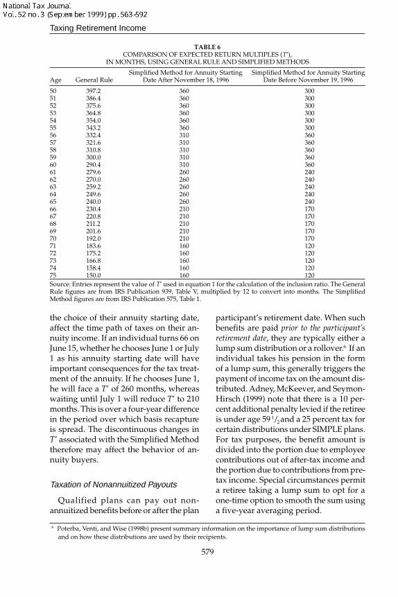
Table 6 shows the value of T’, in months,for both the General Rule and the Simpli-fied Method. The first column of Table 6is the age of the annuitant when annuitypayouts begin. The second column is thevalue of T’ under the General Rule. Thethird column is the value of T’ for the Sim-plified Method for those annuities start-ing after November 18, 1996. This is thecolumn that will apply to most qualifiedannuities from today forward. The fourthcolumn is the value of T’ for the Simpli-fied Method for those annuities subject tothe Simplified Method, but with startingdates before November 19, 1996.

As discussed earlier, raising the valueof T’ has two offsetting effects on the af-ter-tax value of an annuity relative to ataxable bond. We have evaluated the sen-sitivity of our EPDV findings to changesin T’ and, in general, find relatively mod-est effects. For example, for a 65-year-oldmale facing a marginal tax rate of 36 per-cent, a shift from a T’ value of 20 years toa value of 21 years raises the inclusionratio from 0.431 to 0.458. This change re-duces the EPDV of an annuity from 0.959to 0.953, or by 0.6 cents per dollar of an-nuity premium.

One potentially significant effect of theSimplified Method, rather than the Gen-eral Rule, is that it makes the tax treatmentof an annuity a function of when the indi-vidual begins receiving payouts. Indi-viduals who are near an “endpoint” ageunder the Simplified Method can, through

5 The Simplified Method must be used if either the annuity starting date is after November 18, 1996 and thepayments are from a qualified plan, or if the annuitant was at least 75 years old when the annuity paymentsbegan, payments were from a qualified plan, and payments were guaranteed for fewer than five years. Allother payments, such as those from nonqualified annuities, must continue to use the General Rule.


579

the choice of their annuity starting date,affect the time path of taxes on their an-nuity income. If an individual turns 66 onJune 15, whether he chooses June 1 or July1 as his annuity starting date will haveimportant consequences for the tax treat-ment of the annuity. If he chooses June 1,he will face a T’ of 260 months, whereaswaiting until July 1 will reduce T’ to 210months. This is over a four-year differencein the period over which basis recaptureis spread. The discontinuous changes inT’ associated with the Simplified Methodtherefore may affect the behavior of an-nuity buyers.

Taxation of Nonannuitized Payouts

Qualified plans can pay out non-annuitized benefits before or after the plan

participant’s retirement date. When suchbenefits are paid prior to the participant’sretirement date, they are typically either alump sum distribution or a rollover.6 If anindividual takes his pension in the formof a lump sum, this generally triggers thepayment of income tax on the amount dis-tributed. Adney, McKeever, and Seymon-Hirsch (1999) note that there is a 10 per-cent additional penalty levied if the retireeis under age 59 1/2 and a 25 percent tax forcertain distributions under SIMPLE plans.For tax purposes, the benefit amount isdivided into the portion due to employeecontributions out of after-tax income andthe portion due to contributions from pre-tax income. Special circumstances permita retiree taking a lump sum to opt for aone-time option to smooth the sum usinga five-year averaging period.

TABLE 6COMPARISON OF EXPECTED RETURN MULTIPLES (T’),

IN MONTHS, USING GENERAL RULE AND SIMPLIFIED METHODS

5051525354555657585960616263646566676869707172737475

397.2386.4375.6364.8354.0343.2332.4321.6310.8300.0290.4279.6270.0259.2249.6240.0230.4220.8211.2201.6192.0183.6175.2166.8158.4150.0

300300300300300300360360360360360240240240240240170170170170170120120120120120

Age General RuleSimplified Method for Annuity Starting

Date After November 18, 1996Simplified Method for Annuity Starting

Date Before November 19, 1996

360360360360360360310310310310310260260260260260210210210210210160160160160160

Source: Entries represent the value of T’ used in equation 1 for the calculation of the inclusion ratio. The GeneralRule figures are from IRS Publication 939, Table V, multiplied by 12 to convert into months. The SimplifiedMethod figures are from IRS Publication 575, Table 1.

6 Poterba, Venti, and Wise (1998b) present summary information on the importance of lump sum distributionsand on how these distributions are used by their recipients.


580

Moving a lump sum to a rollover Indi-vidual Retirement Account (IRA) does nottrigger immediate tax payments. An em-ployer must withhold 20 percent of arollover, however, unless the recipientchooses to have the funds transferred di-rectly to a tax qualified retirement plan.In the case of a successful tax-free rollover,at some point, the retiree would be re-quired to begin receiving the rolloverfunds in accordance with minimum dis-tribution rules described below.

With respect to nonannuitized benefitspaid to retirees, it is worth emphasizingthat historically, most qualified pensionplans offered only annuity benefits andprohibited all other payout alternatives.Today, however, many pension plan par-ticipants have some choice about the formof their pension payout. The U.S. Bureauof Labor Statistics (1998) reports that 85percent of private defined contributionpensions currently offer lump sums to re-tirees, and 15 percent of private definedbenefit pensions do so as well. In fact, an-nuity payouts are apparently available toonly 17 percent of private sector definedcontribution pension participants, under-scoring the importance of nonannuitypayout options.

Minimum Distribution Rules

The expanding set of options for tak-ing distributions from qualified accountsmeans that a qualified pension plan par-ticipant who does not want to take a lumpsum or rollover, and who chooses not topurchase an annuity, must, and increas-ingly does, turn to a nonannuitized pay-

out formula. Tax law holds that these ben-efits must be paid out under “minimumdistribution requirements.” Retirementplan payouts must start at least by a speci-fied time and may continue periodically,at least annually, over the relevant livesor life expectancies of the plan participantand his designated beneficiary.7 Theserequirements were first adopted in 1962when there were no limits on contribu-tions to retirement plans and plan assetswere not counted in taxable estate. Theirgoal was mainly to prevent Keogh plans,used frequently by professionals, frombecoming vehicles for income and estatetax avoidance. Coverage by the require-ments was expanded to all types of retire-ment plans in 1984 and 1986.

The date at which minimum distribu-tions must begin, relative to life expectancyof those receiving such distributions, hasdeclined significantly since these regula-tions were introduced. Bell, Wade, andGoss (1992) report that life expectancy forthe average 30-year old man in 1960 was70.45 years. Hence, the age of 70 1/2 mighthave been deemed a reasonable age bywhich to expect retirees to begin taking dis-tributions. Today, however, the life expect-ancy of a 30-year-old man is 74 1/2 years.Life expectancy for a 30-year-old womanis 80.8 years, and the labor force today in-cludes a much higher fraction of womenthan it did in 1960. Thus, minimum distri-bution requirements today apply to manymore years of retirement, on average, thanthey did when they were introduced.

Current federal minimum distributionrequirements indicate the minimumamount that must be distributed each year

7 Federal minimum distribution requirements include basic and incidental benefit rules appearing in Section401(a)(9) of the Internal Revenue Code as well as the very detailed proposed Treasury Regulations 1.401(a)(9)-1 and 2. The requirements currently apply to all types of tax-advantaged retirement arrangements, including401(a) plans (defined benefit and money purchase pension plans and profit sharing and stock purchase plans(including 401(k) plans)), 403(b) plans (defined contribution plans available to workers in nonprofit institu-tions and public schools), 457 plans (nonqualified deferred compensation plans available to workers in gov-ernmental bodies), and individual retirement arrangements (Keogh plans and IRAs). The regulations con-strain, in variuos ways, plan design for the annuity payout form. In this paper, however, we concentrate onthe impact of the minimum distribution requirements on nonannuitized payouts. Warshawsky (1998) de-scribes other issues in some detail.


581

to a plan participant and when paymentsmust begin, regardless of whether thepayments are made as a lump sum with-drawal, a series of systematic paymentsover a period of time, or a life annuity. Forexample, if the retiree turned 70 1/2 on Oc-tober 1, 1997, he would have to begin re-ceiving minimum distributions from thepension no later than April 1, 1998. If aplan participant fails to receive qualifiedplan benefits at a rate at least equal to theminimum required amount during theyear, he would be liable for an excise taxequal to 50 percent of the difference be-tween the required payments and the ac-tual payments. If the amount distributedexceeds the minimum required in any cal-endar year, no credit may be recognizedin subsequent years for such excess dis-tribution.8

A plan participant may elect to receivebenefit payouts over his life expectancy.In this event, the minimum required pay-ment is determined every year by divid-ing the accumulation by the applicable lifeexpectancy factor. One other person’s lifeexpectancy can also be included in the fac-tor, and the calculation is then based onthe joint life expectancy of the participantand that other person, subject to certainlimitations. If such a “designated benefi-ciary,” in the language of the regulations,is not selected, payments are based on thesingle life expectancy of the participant,calculated using the IRS unisex mortalitytable that we described above.

A plan participant may choose bothprimary and contingent beneficiaries.Primary beneficiaries receive the accumu-lation remaining upon the death of the

participant, and contingent beneficiariesreceive benefits only if there are no pri-mary beneficiaries remaining alive anda residual accumulation exists. If a planparticipant names several primary benefi-ciaries, only the oldest one can be the cal-culation beneficiary. If a trust satisfies cer-tain conditions, its oldest beneficiary canserve as a calculation beneficiary. Anyonemay be designated as the calculation ben-eficiary, but if he is not the participant’sspouse, the “incidental benefit rule” lim-its the maximum age difference to 10 yearsin calculating the joint life expectancy.

If a retiree holds assets in an individualaccount plan such as a 401(k) plan or IRA,the participant may choose, at the time ofthe first distribution, between two meth-ods of calculating his life expectancy andthat of his designated beneficiary. (Thedesignated beneficiary is also known asthe calculation beneficiary.) Under the re-calculation method, which is available toa participant and to his spouse if thespouse is the calculation beneficiary, theactual age-appropriate life expectancy fac-tor is used each year. For example, for anindividual with no calculation beneficiary,the life expectancy factor is 15.3 at age 71,14.6 at age 72, 13.9 at age 73, and so on. Incontrast, under the one-year-less method,which is available to a participant and toany type of calculation beneficiary, oneyear is subtracted from the original lifeexpectancy factor as he ages. For example,for a recipient with no calculation benefi-ciary, the factor is 15.3 at age 71, 14.3 atage 72, 13.3 at age 73, and so on. The lifeexpectancy factors under either the recal-culation or one-year-less method are ap-

8 These rules apply when payments were begun prior to the death of the plan participant. If, however, theparticipant dies before minimum distributions have begun, the entire accumulation must generally be dis-tributed by the end of the fifth year from the date of the participant’s death. An exception to this general ruleallows for the accumulation to be paid over the life or period of life expectancy of the designated beneficiaryif elected by December 31 of the year after the year of death of the plan participant. For spouses, distributionsunder the exception must commence before the later of (a) the last day of the year following the participant’sdeath or (b) the last day of the year the participant would have attained age 70 1/2 (regardless of the spouse’sage). Either the recalculation or one-year-less method (described below) may be used. Again, rollover to anIRA is allowed. For other beneficiaries, the benefits must commence by the last day of the year following theparticipant’s death. Only the one-year-less method may be used by nonspouse beneficiaries.


582

plied to the account balance as of the lastvaluation date in the prior calendar year,adjusted for any contributions, allocatedforfeitures, and distributions made in theprior year after the last valuation date.Under the one-year-less method, the goalis to distribute the entire retirement assetby the age of (joint) life expectancy,whereas under the recalculation method,payments can continue, albeit in dwin-dling amounts, until the last age in the IRSmortality table.

Minimum distribution rules can affectmany aspects of assets draw-down by re-tirees. These effects are discussed in de-tail in Warshawsky (1998), but we sum-marize them here. First, for the significantminority of elderly individuals who arestill working at age 70 1/2 , the current rulesrequire them to begin taking distributionsfrom IRA and prior-employer’s plans,even though they may still be contribut-ing to their current pension plans.

Second, these rules create awkwardsituations when a spouse, who surviveda plan participant who had not yet re-ceived distributions from the plan, mustinitiate payments no later than the datethe participant would have turned 70 1/2 ,regardless of the surviving spouse’s ageor labor force status. Spouses in this set-ting could roll over pension accumula-tions into an IRA and postpone distribu-tions until they reach age 70 1/2 , but it isnot clear how many spouses are aware ofthis option and pursue it.

Third, one consequence of using aunisex life table in the calculation of mini-mum required distributions is thatwomen, who have longer life expectan-cies as a group, must receive higher dis-tributions than would be consistent witha female-only life table. For example, atage 71, the life expectancy factor for a

woman is 17.2 under the Annuity 2000table, nearly two years more than underthe IRS table.

Finally, minimum distribution rulesmay affect retirees’ patterns of consump-tion spending in retirement. It is difficultto evaluate such linkages, because we arenot aware of any direct evidence on therelationship between payouts from retire-ment plans and the level of householdexpenditures for those who are subject tominimum distribution rules. If a couplechooses to consume their minimum dis-tributions as they are paid out, however,there is a nontrivial risk that at least onespouse will outlive their retirement assets.Minimum distribution requirements mayalso reduce the amount held in tax-de-ferred accounts faster than an accountbeneficiary might otherwise desire. Ifsomeone wishes to consume more in thelater years of retirement than in the earlyyears, he will want to hold a large balanceof assets in tax-deferred (and thereforehigh return) form at the beginning of re-tirement. The minimum distribution rulesmay reduce the level of consumption latein retirement for such an individual bylowering his tax-deferred asset balanceearly in retirement. This effect is particu-larly powerful in inflationary times whenminimum distribution rules are specifiedin nominal terms, as they are at present.9

THE QUANTITATIVE IMPORTANCE OFMINIMUM DISTRIBUTION RULES

A number of current legislative propos-als call for modifying minimum distribu-tion rules by raising the age of mandatorydistribution, updating the mortality tableused in the distribution methods to rec-ognize recent mortality improvements,and/or exempting from the requirements

9 Defined benefit plans may adjust periodic payments upward to reflect price inflation, and variable annuitiesare allowed to adjust payments to reflect changes in the asset values underlying the annuity. Warshawsky(1998) argues that optimal consumption rules would produce distributions that dissipated assets at a slowerrate than under the current one-year-less method and along a different path than under the current recalcula-tion method.


583

individuals with accounts below certainamounts. These proposals would reducethe number of retirees who are affectedby the current minimum distributionrules. In the short run, this could lead to areduction in the amount of distributionsfrom qualified accounts, in turn reducingincome tax collections on qualified ac-count distributions. The longer-term effecton revenues is more difficult to evaluate,because some of the assets that are notdistributed from qualified plans in thenear term will need to be distributed inthe future.

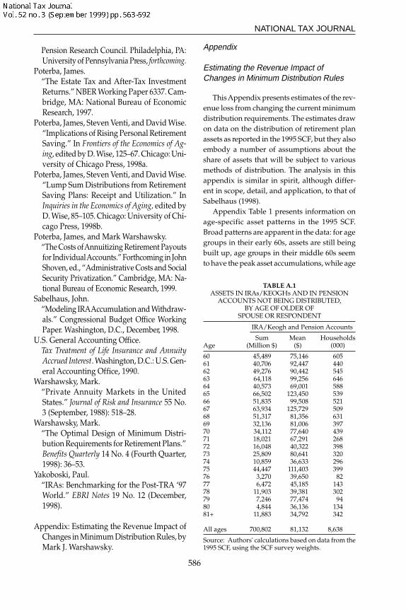
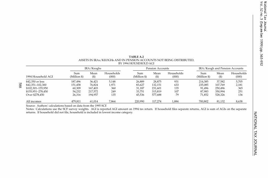
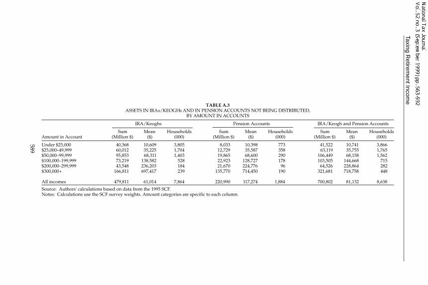
To evaluate the economic significanceof changing the minimum distributionrequirements and to begin the process ofestimating the revenue effects of suchchanges, we need to explore the numberof individuals who are affected by theserules and the value of their qualified ac-count balances. Unfortunately, there is nonationally representative database on theextent of forced distributions that are dueto the minimum distribution rules. Esti-mating the potential revenue effects ofreforming the minimum distribution re-quirements therefore requires drawing ondata from a variety of different sources toproject future retirement assets by age ofhousehold, by household marginal taxrate, and by account balance. These datamust also be used to predict which indi-viduals will be constrained by the currentrequirements. The Appendix presents cal-

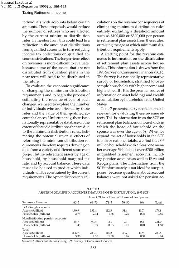
culations on the revenue consequences ofeliminating minimum distribution rulesentirely, excluding a threshold amountsuch as $100,000 or $300,000 per personin retirement plan assets from these rules,or raising the age at which minimum dis-tribution requirements apply.

A starting point for the revenue esti-mates is information on the distributionof retirement plan assets across house-holds. This information is drawn from the1995 Survey of Consumer Finances (SCF).The Survey is a nationally representativesurvey of households, stratified to over-sample households with high income andhigh net worth. It is the premier source ofinformation on asset holdings and wealthaccumulation by households in the UnitedStates.

Table 7 presents one type of data that isrelevant for evaluating these revenue ef-fects. This is information from the SCF onretirement plan balances of households inwhich the head of household or thespouse was over the age of 59. When weexpand the set of households in the SCFto mirror national totals, we find that 8.6million households with at least one mem-ber over age 59 held just over $700 billionin qualified retirement accounts, includ-ing pension accounts as well as IRAs andKeogh plans. The information from theSCF unfortunately is not ideal for our pur-poses, because questions about accountbalances were not asked for pension ac-

IRA/Keogh accountsAssets ($billion)Households (million)

Nondistributing pension accountsAssets ($ billion)Households (million)

TotalAssets ($billion)Households (million)

190.92.75

115.71.45

306.73.36

133.42.34

99.90.39

233.32.50

112.31.68

2.90.03

115.21.68

31.40.76

2.30.01

33.70.76

11.70.34

0.20.01

11.90.34

479.87.86

221.01.88

700.88.64

Source: Authors’ tabulations using 1995 Survey of Consumer Finances.

TABLE 7ASSETS IN QUALIFIED ACCOUNTS THAT ARE NOT IN DISTRIBUTION, 1995 SCF

Summary Measure

Age of Older of Head of Household or Spouse

60–5 66–70 71–5 76–80 80+ Total


584

counts if the account was already in dis-tribution. For respondents over the age of71, this essentially eliminates informationon pension accounts, because the mini-mum distribution rules require payoutsfrom these accounts. The table neverthe-less shows that households in which theoldest member was between the ages of66 and 70 held $233.3 billion in assets in1995. This is the pool of assets that aremost likely to be affected by the minimumdistribution requirements.

CONCLUSIONS AND FUTUREDIRECTIONS

This study has assessed the current taxtreatment of payouts from retirement as-sets, focusing on nonqualified annuityproducts and qualified retirement plans.We explore the economic effects of currenttax rules, and we find that the current sys-tem does not substantially alter the rela-tive attractiveness of taxable bonds andannuity products. We also show how asimpler method of taxing annuities wouldavoid changing the tax rules as an annu-itant aged while still raising the same ex-pected present discounted value of rev-enues as the current tax rules. With respectto qualified plan payouts, we first con-sider annuitized payouts and then outlinethe minimum distribution requirementsassociated with nonannuitized payouts.We note that minimum distribution ruleswere initially implemented in an eco-nomic and demographic environmentthat was different from the current settingand that such rules may have a numberof initially unintended effects on currentretirees.

Our current analysis suggests severaldirections for further work. One is tomove beyond the present discussion ofincome tax issues to consider estate taxissues as well. While Poterba (1997) re-ports that the estate tax currently appliesto less than two percent of all decedents,estate tax rates are higher than the income

tax rates facing most households. The es-tate tax therefore could have substantialeffects on the behavior of those high networth households who may be subject toit.

A second direction for further work con-cerns the utility consequences of mini-mum distribution rules. We have de-scribed the operation of these rules, butwe have not tried to link these rules to theconsumption flow available to retirees.While our analysis of annuities uses anexplicit utility function to compare a rep-resentative household’s lifetime expectedutility under various annuity tax regimes,we have not tried to apply such a frame-work to minimum distribution rules. Thisextension is not straightforward, becauseit requires assumptions about the link be-tween required distributions and house-hold consumption. Future work couldusefully explore both this link and thecorresponding impact of minimum distri-bution rules on household welfare.

A third limitation of our current analy-sis is our focus on the choice between tax-able bonds and taxable annuities. House-holds in practice face a much wider menuof investment choices, many of which aretaxed less heavily than taxable bonds. Thecomparison between annuities and corpo-rate stock, which generate part of theirreturn in the form of capital gains, wouldbe particularly interesting. This is espe-cially true for high-income households,facing a marginal tax rate of 36 or 39.6percent on interest and annuity income.For these households, the top marginal taxrate of 20 percent on long-term capitalgains could have an important impact onthe choice between annuities and capitalassets that are expected to appreciate.

A final direction for further analysisconcerns potential changes in the mortal-ity tables that the IRS uses for annuityvaluation. Changes to these mortalitytables affect the after-tax payouts fromannuities through changes in the expectedreturn multiple, T’. We noted that such


585

changes have two effects: they change thefraction of annuity payouts that are in-cluded in taxable income when the inclu-sion ratio is not 100 percent, and theychange the number of months or yearsover which the inclusion ratio is less than100 percent. A quantitative frameworksuch as the one we have developed is veryhelpful in evaluating the net impact ofsuch changes on the relative attractivenessof annuities and other taxable investments.

Acknowledgments

We are grateful to Norman Greenbergof the IRS for providing us with informa-tion about IRS mortality tables, to JohnAmeriks of the TIAA-CREF Institute forassistance with the SCF, and to Peter Dia-mond and Emil Sunley for helpful com-ments. Poterba and Brown thank the Na-tional Science Foundation, the NationalInstitute on Aging, and the SmithRichardson Foundation for research sup-port; Mitchell acknowledges support fromthe Pension Research Council. This re-search is part of the NBER Programs onAging and Public Economics. The viewsexpressed are solely those of the authors.

REFERENCES

Adney, John T., Joseph F. McKeever, andBarbara N. Seymon-Hirsch.

Annuities Answer Book. A Panel Publication.New York: Aspen Publishers, Inc., 1999.

Bell, Felicitie, A. Wade, and S. Goss.“Life Tables for the United States Social Se-curity Area 1900–2080.” Actuarial Study No.107. Social Security Administration, Officeof the Actuary, 1992.

Brown, Jeffrey, Olivia Mitchell, and JamesPoterba.

“The Role of Real Annuities and IndexedBonds in an Individual Accounts RetirementProgram.” Forthcoming in John Campbelland Martin Feldstein, eds., Risk Aspects ofSocial Security Reform. Cambridge, MA: Na-tional Bureau of Economic Research, 1999.

Bureau of Labor Statistics.Employee Benefits in Medium and Large Pri-vate Establishments. 1995. U.S. Departmentof Labor Bulletin 2496, April, 1998.

Committee to Recommend a New MortalityBasis for Individual Annuity Valuation.

“Report (Derivation of the 1983 Table a).”Transactions of the Society of Actuaries. 33(1981): 675–751.

Friedman, Benjamin, and Mark Warshawsky.“Annuity Prices and Saving Behavior in theUnited States.” In Pensions in the USEconomy, edited by Z. Bodie, J. Shoven, andD. Wise, 53–77. Chicago: University of Chi-cago Press, 1988.

Friedman, Benjamin, and Mark Warshawsky.“The Cost of Annuities: Implications forSaving Behavior and Bequests.” QuarterlyJournal of Economics 105 No. 1 (February,1990): 135–54.

Individual Annuity Experience Committee.“Report: Mortality Under Individual Imme-diate Annuities, Life Income Settlements,& Matured Deferred Annuities Between 1976& 1986 Anniversaries.” Transactions of the So-ciety of Actuaries: 1991–2 Reports, 65–116.

Johansen, R.“Review of Adequacy of 1983 Individual An-nuity Mortality Table.” Transactions of theSociety of Actuaries 47 (1996): 101–23.

McGill, Dan, John Haley, Kyle Brown, andSylvester Schieber.

Fundamentals of Private Pensions 7e. Philadel-phia: University of Pennsylvania Press, 1996.

Mitchell, Olivia S., and David McCarthy.“The Structure and Performance of State andLocal Pension Plans.” Pension ResearchCouncil Working Paper. Philadelphia:Wharton School, April 1999.

Mitchell, Olivia S., James Poterba, MarkWarshawsky, and Jeffrey Brown.

“New Evidence on the Money’s Worth of In-dividual Annuities.” American Economic Re-view. (forthcoming, 1999).

Moore, James, and Olivia S. Mitchell.“Projected Retirement Wealth and SavingAdequacy.” In Forecasting Retirement Needsand Retirement Wealth, edited by O.S.Mitchell, B. Hammond, and A. Rappaport.


586

Pension Research Council. Philadelphia, PA:University of Pennsylvania Press, forthcoming.

Poterba, James.“The Estate Tax and After-Tax InvestmentReturns.” NBER Working Paper 6337. Cam-bridge, MA: National Bureau of EconomicResearch, 1997.

Poterba, James, Steven Venti, and David Wise.“Implications of Rising Personal RetirementSaving.” In Frontiers of the Economics of Ag-ing, edited by D. Wise, 125–67. Chicago: Uni-versity of Chicago Press, 1998a.

Poterba, James, Steven Venti, and David Wise.“Lump Sum Distributions from RetirementSaving Plans: Receipt and Utilization.” InInquiries in the Economics of Aging, edited byD. Wise, 85–105. Chicago: University of Chi-cago Press, 1998b.

Poterba, James, and Mark Warshawsky.“The Costs of Annuitizing Retirement Payoutsfor Individual Accounts.” Forthcoming in JohnShoven, ed., “Administrative Costs and SocialSecurity Privatization.” Cambridge, MA: Na-tional Bureau of Economic Research, 1999.

Sabelhaus, John.“Modeling IRA Accumulation and Withdraw-als.” Congressional Budget Office WorkingPaper. Washington, D.C., December, 1998.

U.S. General Accounting Office.Tax Treatment of Life Insurance and AnnuityAccrued Interest. Washington, D.C.: U.S. Gen-eral Accounting Office, 1990.

Warshawsky, Mark.“Private Annuity Markets in the UnitedStates.” Journal of Risk and Insurance 55 No.3 (September, 1988): 518–28.

Warshawsky, Mark.“The Optimal Design of Minimum Distri-bution Requirements for Retirement Plans.”Benefits Quarterly 14 No. 4 (Fourth Quarter,1998): 36–53.

Yakoboski, Paul.“IRAs: Benchmarking for the Post-TRA ‘97World.” EBRI Notes 19 No. 12 (December,1998).

Appendix: Estimating the Revenue Impact ofChanges in Minimum Distribution Rules, byMark J. Warshawsky.

Appendix

Estimating the Revenue Impact ofChanges in Minimum Distribution Rules

This Appendix presents estimates of the rev-enue loss from changing the current minimumdistribution requirements. The estimates drawon data on the distribution of retirement planassets as reported in the 1995 SCF, but they alsoembody a number of assumptions about theshare of assets that will be subject to variousmethods of distribution. The analysis in thisappendix is similar in spirit, although differ-ent in scope, detail, and application, to that ofSabelhaus (1998).

Appendix Table 1 presents information onage-specific asset patterns in the 1995 SCF.Broad patterns are apparent in the data: for agegroups in their early 60s, assets are still beingbuilt up, age groups in their middle 60s seemto have the peak asset accumulations, while age

TABLE A.1ASSETS IN IRAs/KEOGHs AND IN PENSION

ACCOUNTS NOT BEING DISTRIBUTED,BY AGE OF OLDER OF

SPOUSE OR RESPONDENT

60616263646566676869707172737475767778798081+

All ages

45,48940,70649,27664,11840,57366,50251,83563,93451,31732,13634,11218,02116,04825,80910,85944,4473,2706,472

11,9037,2464,844

11,883

700,802

75,14692,44790,44299,25669,001

123,45099,508

125,72981,35681,00677,64067,29140,32280,64136,633

111,40339,65045,18539,38177,47436,13634,792

81,132

60544054564658853952150963139743926839832029639982

14330294

134342

8,638

Source: Authors' calculations based on data from the1995 SCF, using the SCF survey weights.

Age

IRA/Keogh and Pension Accounts

Sum(Million $)

Mean($)

Households(000)


587

groups in their late 60s and beyond (who arealso shrinking in numbers) have declining as-set balances. As will be explained further be-low, the key number in the revenue estimatemodel is retirement assets held by householdsage 70. Looking at Table 7 and Appendix Table1 together, our rough estimate is $35 billion in1995 for this single age group. Appendix Table2 shows retirement account assets by house-hold adjusted gross income (AGI) in 1994. Thefive income groups shown delineate the fed-eral income tax brackets in 1998 for marriedcouples filing joint tax returns (correspondingmarginal tax rates are 15, 28, 31, 36, and 39.6percent). Over two-thirds of the older house-holds with retirement accounts are in the low-est income group, holding almost one-third ofthe retirement assets. The next two groups, rep-resenting middle- and upper-middle-classhouseholds, number more than a quarter of allolder households with retirement accounts andthey hold nearly half of all retirement assets.Finally, the upper-income group accounts forabout one-twelfth of the population and itholds over one-sixth of the retirement assets.

It is necessary to know how retirement as-sets are distributed, and how household AGIsand hence effective tax rates vary, in order toestimate potential revenue losses from changesin the minimum distribution requirements. Theanalysis continues by examining how retire-ment account assets vary by level and income.Appendix Tables 3 and 4 report this informa-tion. Roughly 40 percent of the relevant olderpopulation holds only one-tenth of all retire-ment assets, totaling under $25,000 per house-hold. By contrast, the top five percent of thepopulation holds almost half the assets,amounting to over $300,000 per household.When IRA, Keogh, and pension assets are cross-tabulated by household AGI, two findings standout. First, as expected, higher income groupshave larger accounts; and second, even low-income households have some retirement assets.

To estimate federal income taxes collectedbecause of the minimum distribution require-ments, it is necessary to forecast the aggregatesum of retirement assets into the future. First,beginning with the age 70 cohort, asset values

from the 1995 SCF are projected to 2000 usingan annual growth rate of 20 percent, reflectingactual increases in defined contribution pen-sions in 1997, 20 percent for 1998, and 10 per-cent for 1999 and 2000. This relies on increasesreported in Table L.119.c of the Flow of FundsAccounts and actual increases in IRAs reportedby Yakoboski (1998). This produces an estimateof $73 billion for assets held in retirement ac-counts by households age 71 in the year 2000.Similar forecasts are computed for aggregateretirement assets in the year 2000 for house-holds age 71–76 and older. While SCF retire-ment assets decline with age, sample sizes aretoo small to provide a precise estimate of wealthdrawdowns by age group. Instead, these draw-downs are estimated by taking the age 70 re-tirement assets in the year 2000 and assumingthat balances will decline by five percent peryear between ages 71 and 75. Retirement as-sets for households age 76 and older are basedon the IRA, Keogh, and pension account assetsreported earlier for that age group, thenincremented by 66 percent (the share of pen-sion assets in total retirement assets for theunder-70 groups) to reflect unreported pensionaccounts being distributed. The 66 percent in-crement for unreported pension accounts prob-ably is an overcorrection because many planparticipants transfer their pension account toan IRA at, or soon after, retirement. Forecastsof the retirement assets of households in theyears 2001 and beyond assume that the assetsof households initially age 70 and younger willgrow from the year 2000 base at an annual rateof 9 1/4 percent, reflecting a 4 1/2 percent real in-vestment return, a 1 1/2 inflation rate, 2 1/4 per-cent growth of contributions to retirement ac-counts, and an increase in the number of house-holds with retirement accounts of 1 percent.Assets of households initially age 71 and olderare also assumed to grow from their respectivebases at a 9 1/4 percent annual rate.

A crucial next step is evaluating the level ofretirement account distributions produced bythe current minimum distribution require-ments in order to assess the counterfactuals ofinterest. There are no nationally representativedata on this statistic, so the calculations are

NAT

ION

AL TA

X JO

UR

NA

L

588

TABLE A.2ASSETS IN IRAs/KEOGHs AND IN PENSION ACCOUNTS NOT BEING DISTRIBUTED,

BY 1994 HOUSEHOLD AGI

$42,350 or less$42,351–102,300$102,301–155,950$155,951–278,450Over $278,450

All incomes

214,385235,08591,49687,98371,852

700,802

37,582107,769250,496350,994528,326

81,132

5,7052,181

365251136

8,638Source: Authors' calculations based on data from the 1995 SCF.Notes: Calculations use the SCF survey weights. AGI is reported AGI amount on 1994 tax return. If household files separate returns, AGI is sum of AGIs on the separatereturns. If household did not file, household is included in lowest income category.

1994 Household AGI


Sum(Million $)

Mean($)

Households(000)

187,496151,45860,30954,23226,316

479,811

36,42176,824

167,403217,572194,957

61,014

5,1481,971

360249135

7,864

IRA/Keoghs

Sum(Million $)

Mean($)

Households(000)

26,88983,62731,18733,75145,536

220,990

28,875132,151231,601315,819577,688

117,274

93163313510779

1,884

Pension Accounts

Sum(Million $)

Mean($)

Households(000)

Taxing Retirem

ent Income

589


BY AMOUNT IN ACCOUNTS

Under $25,000$25,000–49,999$50,000–99,999$100,000–199,999$200,000–299,999$300,000+

All incomes

41,52263,119

106,449103,50564,526

321,681

700,802

10,74135,75568,158

144,668228,864718,758

81,132

3,8661,7651,562

715282448

8,638

Amount in Account


Sum(Million $)

Mean($)

Households(000)

40,36860,01295,85373,21943,548

166,811

479,811

10,60935,22568,311

138,582236,203697,417

61,014

3,8051,7041,403

528184239

7,864

IRA/Keoghs

Sum(Million $)

Mean($)

Households(000)

8,03312,72919,86522,92321,670

135,770

220,990

10,39835,58768,600

128,727224,776714,450

117,274

77335829017896

190

1,884

Pension Accounts

Sum(Million $)

Mean($)

Households(000)

Source: Authors' calculations based on data from the 1995 SCF.Notes: Calculations use the SCF survey weights. Amount categories are specific to each column.


590

based on information from TIAA-CREF show-ing that about 20 percent of the retirementaccumulations are subject to minimum distri-bution requirements each year; the other 80 per-cent are distributed as life annuities, lump sumwithdrawals, and systematic withdrawals. Itseems reasonable to assume that a quarter ofthe accounts currently being distributed ac-cording to the minimum rules will not be helduntil the death of the plan participant andspouse, but instead will be distributed in somefashion over the retirement years. Furthermore,some proportion of the assets in the accountswill be distributed upon the death of thecouples holding the accounts. Lacking betterempirical information, the calculations assumethat 15 percent of IRA, Keogh, and pension ac-cumulations are forced distributions that aredue to the federal requirements. Also, we makea reasonable assumption in the revenue esti-mation procedure that forced distributions aremore likely as income increases; in particular,we assume that 10, 12.5, 15, 20, and 30 percentof retirement account assets are distributedcurrently because of the minimum distributionrequirements currently in effect. Applying thesepercentages to the proportion of retirement as-sets held by each income group shown in Table7 yields a share of about 15 percent of assetsthat would be inferred to be distributed as aresult of the federal requirements. These forceddistributions are then multiplied by effectivetax rates assumed for each of the five incomegroups identified above, assumed to be 10, 20,

25, 30, and 35 percent, respectively. Finally,potential tax revenue generated by the currentminimum distribution rules is estimated bysumming across the projected populations byage and income. This is also summed over theten-year period beginning in 2000.

If the minimum distribution rules were re-pealed, the estimated revenue loss would beestimated to be approximately $21 billion overten years. Because retirement assets are as-sumed to grow over time, the annual foregonerevenue also grows. Lost revenues are esti-mated at about $13 billion over ten years if theminimum distribution rules are changed to ex-clude the first $300,000 in peoples’ retirementplans. This proposal is similar in spirit to a pen-sion reform bill previously proposed by Rep-resentatives Portman and Cardin (H.R. 3788);such a rule change would protect nearly 8 mil-lion older households from having to complywith the minimum distribution regulations.Households holding over $300,000 in their ac-counts would still pay tax on about 58 percentof retirement assets [=(321.7 – (448 * 0.3))/321.7of retirement assets for the households in thecategory labeled “$300,000+” mainly includingthe top four income groups]. These estimatesassume that the exclusion amounts are indexedto expected returns.

Revenue losses would be about $8 billionover ten years if the minimum distributionrules applied only to assets over $100,000 in re-tirement accounts; this would enable almost 6million households to avoid the computations


BY AMOUNT IN ACCOUNTS AND 1994 HOUSEHOLD AGI

Under $25,000$25,000–49,999$50,000–99,999$100,000–199,999$200,000–299,999$300,000+

All incomes

Amount in Account

31,47845,13267,72335,30316,65218,098

214,385

$42,350 or less

8,13215,50731,89744,58038,06796,901

235,085

$42,351–$102,300

1,5121,6071,4528,2033,102

75,621

91,496

$102,301–$155,950

317358

3,6988,7475,667

69,195

87,983

$155,951–$278,450

83515

1,6796,6711,038

61,866

71,852

Over$278,450

41,52263,119

106,449103,50564,526321,681

700,802

AllIncomes

Notes: Authors' calculations based on data from the 1995 SCF, using the SCF survey weights. AGI is reportedAGI amount on 1994 tax return. If household files separate returns, AGI is sum of AGIs on the separate returns.If household did not file, household is included in lowest income category.

1994 Household AGI


591

associated with minimum distribution rules.(This is similar to the pension reform bill intro-duced by Representatives Portman and Cardinin the current Congress, but we abstract fromthe actual language of current bills (e.g., H.R.1102) inasmuch as they set a cap of $100,000 onexclusions for IRAs and pension accounts sepa-rately.) However, older households would stillhave to determine which part of their retire-ment assets were subject to the minimum dis-tribution rules, if any. Further, it is unclearwhether households whose account balanceswere just below the exclusion amount whenthey turned age 70 1/2 , but whose account bal-

ances later rose above the exclusion due to su-perior investment returns, would later becomesubject to the minimum distribution require-ments. Revenue losses would be only $8.5 bil-lion over ten years if the minimum distribu-tion requirements were delayed to householdsage 75, as proposed in a bill introduced in thecurrent Congress by Senators Grassley andGramm. The model assumes that the lawchange would apply to those currently receiv-ing distributions between the ages of 70 1/2 and75; that is, these older individuals would notbe forced to continue to take distributions un-til they turned age 75.

Date post:	05-May-2018
Category:	Documents
Upload:	vuongdieu
View:	216 times
Download:	1 times

Taxing Retirement Income: Nonqualified Annuities … taxation of retirement saving is an important...

Documents