AFATL-TR-89-41 Taylor Impact Testing AD-A215 018 J W House UNIVERSITY OF KENTUCKY LEXINGTON, KENTUCKY, 40506-0046 DTVC SEPTEMBER 1989 ELECTE SP B 1SEP2519, FINAL REPORT FOR PERIOD JUNE 1987 JANUARY 1989 APPROVED FOR PUBLIC RELEASE; DISTRIBUTION UNLIMITED AIR FORCE ARMAMENT LABORATORY Air Force Systems Commandl United States Air Force IIEglin Air Force Base, Florida 89 9 25 018
Transcript
AFATL-TR-89-41
Taylor Impact Testing AD-A215 018
J W House
UNIVERSITY OF KENTUCKY
LEXINGTON, KENTUCKY, 40506-0046
DTVCSEPTEMBER 1989 ELECTE
SP B 1SEP2519,
FINAL REPORT FOR PERIOD JUNE 1987 JANUARY 1989
APPROVED FOR PUBLIC RELEASE; DISTRIBUTION UNLIMITED
AIR FORCE ARMAMENT LABORATORYAir Force Systems Commandl United States Air Force IIEglin Air Force Base, Florida
89 9 25 018
I
NOTICE
When Government drawings, specifications, or other data are used for anypurpose other than in connection with a definitely related Government procure-ment operation, the United States Government thereby incurs no responsibilitynor any obligation whatsoever; and the fact that the Government may have formu- h
lated, furnished, or in any way supplied the said drawings, specifications, orother data, is not to be regarded by implication or otherwise as in any mannerlicensing the holder or any other person or corporation, or conveying anyrights or permission to manufacture, use, or sell any patented invention thatmay in any way be related thereto.
The AFATL STINFO program manager has reviewed this report, and it isreleasable to the National Technical Information Service (NTIS). At NTIS,it will be available to the general public, including foreign nations.
This technical report has been reviewed and is approved for publication.
FOR THE COMMANDER
WARD J. BUSH. COL. USAFhief, Munitions Division
If your address has changed, if you wish to be removed from our mailinglist, or if the addressee is no longer employed by your organization, pleasenotify AFATL/MNW , Eglin AFB FL 32542-5434.
Copies of this report should not be returned unless return is required bysecurity ccisiderations, contractual obligations, or notice on a specificdocument.
Unclassified2a. SECURITY CLASSIFICATION AUTHORITY 3. DISTRIBUTION /AVAILABII ITY OF REPORT
Approved for public release;2b. DECLASSIFICATION /DOWNGRADING SCHEDULE distribution is unlimited
4. PERFORMING ORGANIZATION REPORT NUMBER(S) S. MONITORING ORGANIZATION REPORT NUMBER(S)
N/A AFATL-TR-89-416a. NAME OF PERFORMING ORGANIZATION 6b. OFFICE SYMBOL 7a. NAME OF MONITORING ORGANIZATIONThe Graduate School of (If applicable) Warheads BLanchUniversity of Kentucky Munitions Division6c. ADDRESS (City, State, and ZIP Code) 7b. ADDRESS (City, State, and ZIP Code)University of Kentucky Air Force Armament LaboratoryLexington KY 40506-0046 Eglin AFB FL 32542-5434
8a. NAME OF FUNDING/SPONSORING 8b. OFFICE SYMBOL 9. PROCUREMENT INSTRUMENT IDENTIFICATION NUMBER
ORGANIZATION (If applicable)
Munitions Division AFATL/MNW F08635 87-C-01258c. ADDRESS (City, State, and ZIP Code) 10. SOURCE OF FUNDING NUMBERS
PROGRAM PROJECT TASK WORK UNITAir Force Armament Laboratory ELEMENT NO. NO. NO ACCESSION NO.Eglin AFB FL 32542-5434 62602F 2502 06 28
11. TITLE (Include Securit e Classification)
Taylor Impact Testing
12. PERSONAL AUTHOR(S)Joel W. House
13a. TYPE OF REPORT |113b. TIME COVERED 114. DATE OF REPORT (Year, Month, Day) 115. PAGE COUNTFinal FROM June 87TO 3n I September 1989 129
16. SUPPLEMENTARY NOTATION
Availability of report is specified on verso of front cover.17. COSATI CODES 18. SUBJECT TERMS (Continue on reverse if necessary and identify by block number)
FIELD GROUP SUB-GROUP Plasticity, yield strength, microstructure, fricture1904 1906 1106 / elasticity ( /
19. ABSTRACT (Continue on reverse if necessary and identify by block number),The reaction of armor to penetration by a projectile is an interesting and important areaof science. To assist the armor and armor penetrator designers, several penetration modelshave been developed. These models require data on the behavior of material under highstrain rate conditions resulting from impact. In a paper published in 1948, G.I. Taylorproposed an impact experiment and concomitant analysis to help interpret dynamic materialbehavior. This experimental technique remains in general use today even though there havebeen many attempts over the years to modify Taylor's analysis of the test. Ultimately,the data obtained from such "Taylor" tests are used in models of penetration.
This report presents a critical discussion of the Taylor test, some of the experimentalsetups for its performance, and one current analysis of the test. In addition, actual
experimental results are presented and analyzed, and the resulting impact induced materialmicrostructures are studied.
20. DISTRIBUTION/AVAILABILITY OF ABSTRACT 21. ABSTRACT SECURITY CLASSIFICATION0 UNCLASSIFIED/UNLIMITED M SAME AS RPT. [3 DTIC USERS Unclassified
2Ud. NdAME u. kESPONSIBLE INUIVIDUAL 22b. TELEPHONE (Incluhdp Area Code) 22c OFFICE SYMBOL
Leonard L. Wilson o
DO Form 1473, JUN 86 Previous editions are obsolete. SECURITY CLASSIFICATION OF THIS PAGEUNCLASSIFIED
PREFACE
This report describes an experimental and analytical approachto the deterrination of dynamic material behavior. Experimentaldata was collected to verify and refine a one-dimensional predic-tive model being developed as a design tool for weapon designers.The work was accomplished under contract F08635-87-C-0125, pro-gram element 62602F, JON 25020628, during the period from June1987 to January 1989. The analytical and metallurgical work wasaccomplished by Mr. Joel W. House at the Graduate School of theUniversity of Kentucky.
The Taylor Impact tests were conducted on Eglin Test SiteC-64B. Mr. Leonard L. Wilson of the Air Force ArmamentLaboratory, Munitions Division, Warhead Branch (MNW) was theprngrar ragcr.
Accession For
TIS CPA&I
CuT;t 1 T' S÷
I i r I but I on,,|Av :ll~b' I~ Codes
AV~fl i and/or
DI i I
iii -'"
Acknowledgement
The author thanks his adviser, Dr. P. P. Gillis; and Dr. S.E. Jones, Dr. J. C. Foster Jr., and Dr. R. J. De Angelis fortheir guidance throughout this investigation.
The author is grateful to Mr. Leonard Wilson. Mr. Wilson'smany years of experience conducting terminal ballistic testswere invaluable to this investigation.
The author is indebted to Kenneth Bcggs for his assistancewith the microstructural investigation.
iv
TABLE OF CONTENTS
Section Title Page
INTRODUCTIONDynamic Material Behavior ........... 1
VII CONCLUSIONS1. Introduction ....... ........... 782. Experimental Apparatus
and Methodology .... ........... 78
v
TABLE OF CONTENTS
Section Title Page
3. Physical Process ResultingFrom impact ...... ............. 79
4. a/p Model ........ .............. 80
REFERENCES ......... ................ 83
BIBLIOGRAPHY ....... ............... .. 84
Appendix
A TEST PROCEDURES ...... ............. 85B DATA FILES ......... ................ 91C TENSILE SPECIMEN. ....................... 99D LOAD VERSUS TIME CHARTS ... ......... 103E HUGONIOT MODEL ....... .............. 109F RAW DATA SHEETS ...... ............. 117
vi
LIST OF FIGURES
Figure Title Page
1 Plastic and Elastic Wave Motion in theSpecimen ................... ... ...... 5
2 Nomenclature Used in the Taylor Analysis. 7
3 Schematic Diagram Showing the Volumeof Material that Passes into thePlastic Zone ....... ................. 8
4 Stress Ratio Contours Used forDetermining, From the Exact Analysis,the Yield Stress .... ............. ... 12
36 Stress/Strain Response of PureCopper Under High Strain-RateConditions .......... ................ 31
C-1 Dimensions of the Tensile Specimen . . . i01
D-! Load Response of OFHC Copper ... ....... 105
D-? Load Response of DPTE Copper ......... .. 106
D-3 Load Response of 6061-T6 Aluminum ..... .. 107
D-4 Load Response of 2024-T4 Aluminum ..... .. 108
E-1 Schematic Diagram Showing the ParametersUsed in the Hugoniot Model ..... ........ il
ix
LIST OF TABLES
TabLe Title Page
1 MECHANICAL PROPERTIES (QUASI-STATIC) 20
2 SPECIMEN DIMENSIONS ........ ............. 34
3 LINEAR REGRESSION AND STATISTICAL DATA 39
4 COMPARISON OF STATIC AND DYNAMIC YIELDSTRESS VALUES ............ ................ 40
5 EXPERIMENTAL TEST DATA ....... ........... 42
6 COMPUTED YIELD STRENGTH VALUES ..... ....... 43
7 MATERIAL COMPOSITION ......... ........... 57
x
SECTION I
INTRODUCTION
DYNAMIC MATERIAL BEHAVIOR
The factors common to any static, or dynamic, stress
analysis problem consist of the following: the specimen
geometry, the loading applied at the boundary, and the material
of the specimen. These three factors will interact to produce
the stress level inside the body. The response of the body to
these stresses is important in most engineering endeavors.
Frequently, a rational engineering design requires the ability
to predict the stresses and material response in each component.
The most common approach to investigating the response of a
material is to fix two of the three factors governing the stress
problem. As an example, in a uniaxial tensile test the specimen
geometry and loading have been standardized. This provides a
uniform basis to compare the third factor, the specimen material.
This test is based upon a straightforward method of calculating
the stress level in the specimen.
There are several limitations to this type of materials
investigation. First, the response of the material to the
complex loadings experienced in service may not be accurately
represented by such a simple test. Second, for some applications
the experimental apparatus cannot provide the necessary loading
requirements seen in service, e.g., high strain rates.
To overcome these restrictions the designer can take either
of the two following approaches: use a large factor of safety,
or proceed on a need to know basis. The former, though widely
used, will not be discussed. The second approach usually begins
by redefining the experimental technique in terms of the specific
problem at hand. This approach is used frequently for
investigating materials response to rapidly applied loads. If
the loading rate and magnitude are sufficiently high, the
material response is called dynamic.
Dynamic material behavior has been characterized by the
presence of inertial effects and wave propagation which affect
the stress distribution inside the specimen. If an impulsive
load, large enough to cause permanent deformation. is applied to
the boundary of a specimen, the stress in the region nearest the
load will be significantly higher than in any other portion of
the body. The deformation which occurs in the specimen can be
modeled by its wave-like motion through the material. If the
deformation takes place rapidly, the particle being displaced
will have some inertial energy. If the inertial energy is large
enough, it can have a significant effect on the final
configuration of the specimen.
Certain aspects of dynamic behavior have been known since the
19th century. British investigators showed that an iron wire
could resist permanent deformation under large loads for short
periods of time. This test proved that a relationship existed
between the yield stress in a material and the rate at which the
load was applied.
In the 1940's, G.I. Taylor, Reference 1, met with some
success at charact- izing this behavior. He proposed an
experiment to measure what was then called the dynamic yield
strength.
The experiment proposed by Taylor has 1-ecome a standard test
in laboratories that study the behavior of materials at high
rates of deformation. The Taylor test consists of impacting a
plane-ended cylindrical projectile against a relatively rigid,
massive anvil. What should come out of the Taylor test is the
2
yield stress level for a material that is rapidly, or
impulsively, loaded. The Taylor test was designed to standardize
the specimen geometry and the loading pattern applied to the
specimen boundary. As previously mentioned, the last component
of the internal stress problem would be the material under
investigation.
One use for the information generated by the Taylor test is
in the development of armor and armor penetrators. Models of the
interaction between a target and a penetrator, References 2 and
3, require that the materials be characterized by their dynamic
strength values. Another use for the Taylor test is as an
accuracy check of two-dimensional computer models of deformation
behavior, References 4 and 5.
The object of this report is fourfold. First, it is to
examine aspects of both two-dimensional and one-dimensional
modeling used with Taylor testing. Second, it is to describe in
detail a recently constructed Taylor test apparatus. Third, it
is to provide an analysis of data obtained experimentally and.
used in the one-dimensional models. Fourth, it is to report on
observations made on the microstructure found in test specimens.
3
SECTION II
ONE-DIMENSIONAL MODELS
1. BACKGROUND
One-dimensional models of the Taylor experiment are used to
calculate the yield stress level of a material from post-test
measurements of specimen deformation. Historically, all
one-dimensional models are based on the analysis developed by
Taylor, Reference 1. Over the years various investigators have
proposed modifications to his analysis by changing the basic
equations or using different types of material constitutive
relationships. Therefore, the discussion of one-dimensional
models should begin with a development of Taylor's original
analysis of the problem.
At impact, a wave of compressive stress will be generated at
the anvil face. If the velocity of the projectile is
sufficiently high, the stress wave will separate into two
components. The first, or leading, component is an elastic
compressive wave, moving through the material at the speed of
sound. The amplitude of the stress level behind the compressive
wave front is below the yield strength of the material. The
second component, a plastic compressive wave, will follow the
elastic compressive wave at a greatly reduced velocity. At the
plastic front the stress level exceeds the yield strength of the
material. The high compressive stress causes severe deformation
to occur in the form of radial motion outward away from the
specimen axis, accompanied by axial shortening of the specimen.
As the event proceeds, the elastic compressive wave will
arrive at the free-end of the specimen, where it is reflected as
a tensile wave of equal magnitude. The tensile wave will move
through the specimen until it encounters the plastic compressive
wave front, located within the specimen, Figure 1, Reference 6.
The motion of the elastic wave and the interaction with the
4
plastic compressive wave will have two important effects. First,the velocity of the plastically undeformed portion of the rod
will be reduced as the elastic wave moves through the material.
Second, the reflected tensile wave will superimpose with the
compressive plastic wave to reduce the overall stress at the
plastic wave front. After repeated occurrences, the motion of
and stress within the specimen will both be reduced to zero.
REFLECTEDI"WAVE 'ENSILE
ANVIL. ANVIL
COMPRMVE -ZERO-- STRESS
STRESS. Y PSSTATIONARY
TE
NCIDENTT --0MPRESS-vE
COMPRESSivE ;LASTIC NAVEPLASTIC WAVEFRONT
(a) (b)
Figure 1. Plastic and Elastic Wave Motion in the Specimen
2. TAYLOR'S ANALYSIS
To construct a model of the impact event, Taylor makes three
assumptions in his analysis: the material stress-strain
relationship is rigid, plastic; radial inertia effects can beneglected; and, a condition of uniaxial stress exists across the
elastic/plastic interface. The relative effects of these
assumptions have stirred numerous debates and papers regarding
the validity of his analysis. The simplicity of the experimental
technique and subsequent reduction of data are incentives to
accept these assumptions. It must, however, be kept in mind by
the user of such data the level of approximation that was used in
the construction of the analysis.
Taylor's analysis relates the altered geometry of the
specimen after impact to the dynamic yield strength of the
material. In this way, Taylor could extract the crucial dynamic
5
strength from only two postmortem measurements of the deformed
specimen. Taylor formulates his analysis through equations thatrelate various kinematic parameters during the impact event, such
as the time required for an elastic wave to travel down the rigid
portion of the specimen and back to the plastic wave front, the
incremental change in the position of the plastic wave front, the
foreshortening of the rigid portion ot the rod, and the
incremental change in the velocity of the undeformed portion of
the rod. By eliminating the speed of sound in the material, he
generates a set of differential equations. These differential
equations define the velocity of the plastic wave, the rate of
foreshortening of the undeformed portion of the rod and its
deceleration.
To begin the development of the analysis by Taylor, it isfirst necessary to define the nomenclature to be used, Figure 2.Let L represent the original length of the specimen, and S, the
time dependent displacement of the undeformed portion of the rod
relative to the initial configuration. At some time after
impact, X represents the extent of the plastic zone relative tothe original configuration. The position of the plastic front
is h, measured relative to the anvil face. The current lengthof the undeformed portion is given by k. A relationship exists
between the time dependent quantities, S, Q, h, and the original
lengthL = S + ( + h)
Differentiating Equation (1) with respect to time gives
0 =S + a + h (2)
or
h = -(S + •) (3)
But S is simply the velocity, v, of the back end of the specimen,
and, h is renamed, X, the Eulerian plastic wave speed, to give
S= -(v + 1) (4)
6
x i-
Xf
I I (C,
h S
Figure 2. Nomenclature Used in the Taylor Analysis
The term, j, describes the rate of foreshortening of the
undeformed section of the rod and can be written
-(V + X) (5)
By applying Newton's second law to the undeformed portion of the
rod the equation of motion can be written as
dv = -Y (6)
dt (pA)
Where Y and p are, respectively, the material yield stress
and mass density.
Taylor continues the analysis by writing equations describing
conservation of mass and momentum across the plastic wave front.
A differential slice of the undeformed portion of the rod, dX,
7
Figure 3, with cross sectional area A0 , crosses the plastic front
and is now contained in the volume described by the new area, A,
and the differential thickness, dh. The elemental length, dX,
can be written in terms of the undeformed section using the
relationship, dX = -dA, Figure 2(a). The equation for the
conservation of mass can be written as
pAdh = pAodX (7)
Dividing both sides by pdt, Equation (7) becomes
Adh = AodX (8)dt dt
After substituting for dX in terms of dU, Equation (8) can be
rewritten as
AX = - Ao0 ) (9)
Substituting from Equation (5) gives
AX = Ao(v + X) (10)
Taylor assumes the material behaves in such a way that when
it crosses the plastic- front it comes to rest instantaneously.
This assumption imposes a condition on the model that describes
the intermediate states of the event as having a strain
discontinuity at the elastic/plastic interface, Figures 1
through 3. This strain discontinuity is created by the
/
QA
Ao1
I
dhl dX
Figure 3. Schematic Diagram Showing the Volume of Material ThatPasses into the Plastic Zone
8
instantaneous change in cross sectional area of the material
passing through the plastic front.
The linear momentum equation is written
pAvdA = Y(A - Ao)dt (11)
The left hand side of the equation is the change of momentum of
the differential element, di, having an initial velocity, v, and
a final velocity of zero. The right hand side is the impulse
term, 6here the force is calculated from the stress in the body,
assumed uniform over the cross section, times the relative
change in area.
To construct an analysis based on the postmortem
measurements of the yield boundary, Taylor must describe the
motion of the elastic/plastic interface. Bg Equat ions
(6), (10), and (11), Taylor showed that the plastic front moves
approximately linearly with time. Having determined this from
the analysis, he subsequently imposes this as a constraint on
the model when developing the expression for the yield stress.
The expression Taylor uses for computing the yield stress is
generated from the equation of motion of the undeformed portion
of the rod, Equation (6). The independent variable, however,
has been changed from that of time to the incremental change in
the length of the undeformed section of the rod. This gives
dv = dv dl =- Y (12)dt di dt (pk)
Equation (5) can be substituted into Equation (12) to give
dv = Y (13)dA pA(v + X)
After separating the variables, integrating and substituting the
appropriate initial and final conditions, the equation becomes
Y in Lf] _1 V2 - VX (14)P LT J 2
9
where Lf is the final length of the specimen.
To eliminate the constant plastic wave speed, X, Taylor
assumes that the rear end deceleration of the rod is also
constant. This assumption allows the duration of the impact
event, T, to be calculated two ways. First, from the assumption
of constant plastic wave speedT = (L I _ (15)
Here the term, If, is the final length of the undeformed segment
of the specimen. Then from the assumption of constant
deceleration
T = 2 (L - Lf) (16)V
Eliminating T between Equations (15) and (16) the plastic wave
speed is determined in terms of the impact velocity and the final
specimen geometry
X = (Lf - If) (17)V 2 (L - if)
Using Equation (17) to eliminate the plastic wave speed in
Equation (14), the yield stress is determined as a function of
density, impact velocity, original length, final undeformed
length, and the final total length. This gives the following
expression for the yield stress:
y = OV2 (L - Lf) 1 (18)2 (L - Lf) In _ifl
3. IMPROVED ANALYSIS BY TAYLOR
In a second approach, Taylor concedes that the rear end
deceleration is not constant. He suggests a more exact measure
of the flow stress can be made by applying a correction factor
to the values determined in the above simplified analysis. This
correction factor is calculated from the error introduced by
assuming that the rear end deceleration was uniform.
i03
To determine the correction factor, Taylor establishes a set
of equations relating the plastic wave speed and the rear end
motion to the length of time for the deformation to occur. This
set of expressions can be solved when If/L and Lf/L are known
quantities. To simplify the process, a graph was constructed
with If/L as the ordinate and Lf/L as the abscissa, Figure 4,
Reference 1. The appropriate correction factor, Y/Y 1 , can be
quickly determined from the coordinate position on the graph.
The term Y1 describes the yield stress calculated by Equation
(18). In general, the more exact analysis will increase the
yield stress level of the material.
Taylor's analysis predicts that the cross sectional area of
the deformed region will vary in a uniform manner. At the
elastic/plastic interface, where the state of stress exceeds the
yield strength of the material, the material will deform
radially an amount which is dependent on the current velocity of
the undeformed segment of the specimen. Taylor imposes the
condition that the deceleration of the rear end be uniform;
therefore, the cross sectional area in the deformed region must
be changing uniformly. In reality, the specimen profile in some
materials will be noticeably nonuniform and will depend greatly
on the strength of the material and the velocity of the impact.
Such discrepancies between predicted deformation geometry and
actual observation is related to the assumptions regarding the
material's stress-strain relationship and to the effect of
radial inertia. A rigid, plastic material behavior model
neglects the effects of complex material behavior at high
strain rates. A more comprehensive constitutive model might
contain terms to predict such phenomena as strain hardening,
In order to conduct the proposed test matrix, a suitable
experimental apparatus was required. Several factors determined
by experience with a compressed air gun made it imperative that
a new apparatus be constructed. The baseline operational
requirements called for a flexible, repeatable, and efficient
system design. The perspective from which the new apparatus was
developed can be better understood following a brief summary of
the configuration and capabilities of the compressed air gun
system.
The Gas gun system was simply a high pressure tank, or
vessel, attached to the breech end of a gun barrel. The muzzle
end of the gun barrel was permanently fixed against the side of
a holding tank. The target was positioned in the holding tank
at a standoff distance of approximately 38 cm from the muzzle.
The operation of the gas gun required several steps. First,
a thin metal diaphragm (bursting disk) was placed over the
discharge orifice of the pressure tank. Next, a specimen was
loaded into the gun barrel, after which the barrel and the
pressure vessel were bolted together, sealing the pressure tankorifice. At this point, the vessel could be pressurized to the
desired level. Once the prescribed pressure level was
established, the diaphragm was punctured, via a mechanical
striker, allowing the pressurized gas to escape and accelerate
the specimen through the barrel.
A number of deficiencies were experienced with the use of
such an apparatus. At best, the gas gun system efficiency was
quite poor. After each shot, it was necessary to unbolt the
pressure tank from the barrel. In addition, it took several
21
minutes to build up the operating pressure needed for the test.
In terms of operational capability, the system had very poor
repeatability.
The lack of repeatability was caused by two main problems:
the bursting disk often ruptured prematurely and variations in
the machining of the specimen allowed gas to escape past the
specimen. For shots made at equal tank pressure, the impact
velocities would vary widely if leakage occurred.
The apparatus had built-in limitations with regard to
flexibility. The pressure vessel had, for safety reasons, an
upper limit of 5.17 MPa. Hence, the total available energy was
fixed. For high density materials, this energy level was not
sufficient for experiments in the desired velocity range.
Often, the lack of adequate energy was manifested by oblique
impact with the target. Since the muzzle and target positions
were fixed, the standoff distance could not be adjusted. For
these reasons, a new apparatus, Figure 7, was developed based on
the use of a smokeless gun powder as a propellant.
2. DESCRIPTION OF THE EXPERIMENTAL APPARATUS
The launch tube was machined from 4340 steel and was centerbored to an inside diameter of 7.620 mm. Two ports were drilled
into the gun barrel near the muzzle. The ports were 2.54 cm
apart and were tapped to receive pressure transducers.
Monitoring the electrical signals of the transducers was one
method of determining the projectile velocity near the muzzle of
the launch tube.
The breech end of the launch tube was chambered to accept a0.308 caliber cartridge case. The bullet and original powder
charge were removed from a 0.308 rifle cartridge so that the
primed cartridge case could be used. In place of the originalpowder charge, a specific quantity of smokeless powder (Red Dot)
22
d16
Figure 7. A Taylor Anvil Test Apparatus
was loaded. The propellant was covered with 'a small wad of cot-
ton. The cotton was packed against the powder and primer of the
cartridge. The function of the cotton was to ensure a uniform
burn rate of the propellant from shot to shot by keeping the
powder charge in place against the primer. The powder charges
used for this work varied from 1 to 5 grains (1 gram = 15.4
grains). By comparison, the normal 0.308 rifle cartridge powder
charge is approximately 40 grains. Consequently, a large portion
of the volume was tilled by the cotton.
To lock the cartridge in the chamber, the launch tube had
been externally threaded to facilitate the mounting of an end cap
on the breech. The end cap contained a through hole for the
firing pin in order to make contact with the cartridge, Figure 8.
Actuation of the firing pin was by means of an electric solenoid,
cor.trolled from the firing room.
23
To prevent the expanding powder gas from leaking past the
specimen, a plastic obturator was used to form a seal. The obtu-
rator was positioned between the cartridge and the specimen,
Figure 8. The end of the obturator nearest the cartridge was
hollowed to facilitate radial expansion of the remaining material
under pressure. Thus, the expanding gas deforms the obturator to
form a seal against the gun bore wall. In this manner, the
energy of the propellant was used entirely for accelerating the
specimen.
EARTIDGE--
SPECIMEN BREECH CAP
OBTURATOR zIFIRING SOLENOID
FRN
Figure 8. Firing Line Components
The launch tube was fixed in position by a set of v-block
mounts. This construction allowed rapid change of the standoff
distance between the muzzle and the target. Typically, the
standoff was in the range of 7 to 20 cm.
The target was a 23-cm diameter, by 20 cm in length, cylinder
of hardened 4340 steel. Both ends were machined parallel and lap
finished. The design of the target and target rest, Figure 9,
24
optimized the available surface area for impact tests. After
each test, the target could be rotated to provide a new surface
for impact. If no permanent deformation occurred in the target
surface, several tests were conducted using the same area of the
anvil. After completing one revolution of the target, the
center line of the cylindrical anvil could be lowered with
respect to the projectile flight line to provide a new surface
area for impact. To lower the target, a layer of the polypropo-
lux base material was removed from under the target rest. This
process of lowering the anvil center line could be continued
until the entire surface area was used. Subsequently, the paral-
lel faces of the anvil could be reversed and the process repeated
prior to remachining. This optimized the available area on the
target and reduced the down time required for remachining and
polishing of the surface.
TARGET RESTAND BASE
r LIGHT SOURCE
Figure 9. Target Design and Photographic Contiguration
The target and the muzzle of the launcher were covered by an
aluminum housing. Two slots were cut into the housing parallel
25
to the flight line of the projectile. These slots were coveredwith 6.35 mm thick plexiglass, providing windows w;hi~h allowedthe incoming projectile and its subsequent deformation to bephotographed. The housing prevented the rebounding projectile
from causing undesirable damage. The inside of the housing waslined to prevent secondary deformation from occurring on thespecimen. However, a large number of specimens were slightlydeformed on the rear end of the projectile because of impactwith the muzzle face of the barrel after rebounding from the
target.
3. VELOCITY MEASUREMENT TECHNIQUES
During the test, as many as three techniques were used todetermine the projectile velocity. As previously mentioned, thegun barrel was instrumented with two piezoelectric pressuretransducers. The outputs from the transducer amplifiers werefed into a dual trace oscilloscope. From the oscilloscope, thetime required for the expanding gas of the propellant to passbetween the two transducers could be measured. Knowing the
time, and the distance between the transducer ports, thevelocity was easily calculated.
A learning period was necessary to determine what thresholdsensitivity level to set on the transducer amplifiers for thevarious pressure levels seen in the barrel. If the amplifierswere set too sensitively, the signal would be erratic, possibly
from the elastic wave in the gun itself. If the sensitivity wasset too low, no response would be obtained. In both cases, thenecessary sensitivity level was always pressure dependent.Eventually, the amount of propellant became the best source of apriori information on how to set the sensitivity level.
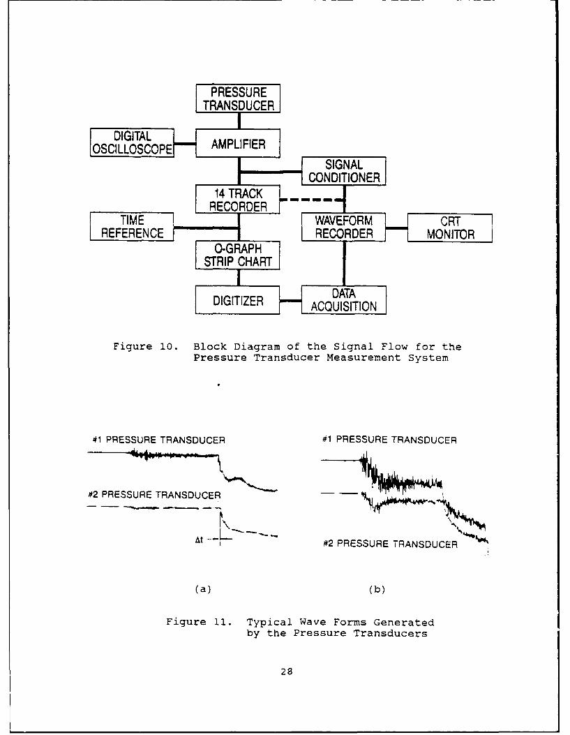
Error in the velocity found by using the pressuretransducers can be analyzed by examining the source for thedata. The signals from the pressure transducers, located near
26
the muzzle end of the launch tube, are sent through a signal
amplifier before being displayed on a digital oscilloscope,
Figure 10. The signals displayed on the oscilloscope can be
measured with the sweep cursor to determine a time interval
necessary for calculating the muzzle velocity, Figure 11(a). It
was considered for this analysis that uncertainties, or
systematic errors, in the measuremert system, i.e., line noise,
transducer and electronic circuit response characteristics, etc.,
were small by comparison to the error introduced by misidentify-
ing the starting and ending points of the interval to be meas-
ured.
The Nicolet oscilloscope displays a digitized form of the
s.gnal as a series of individual points. Each point represents
a segment of time, which for this study was 1 As. The total
time displayed could vary depending on the necessary resolution.
A desirable wave form would show a smooth baseline, before the
obturator passes the transducer port, followed by a sharp point,
the response of the transducer to the propellant gas pressure,
Figure 11(a). A poor signal would have a slowly changing
response, or curved wave form, prior to a rapid deflection,
Figure 11(b).
The former type of signal would provide the necessary infor-
mation to determine the time -a o i 2 As. The accu-
racy from a measurement of a projectile having a velocity of 200
m/s, using this type of wave form would be t3 m/s. The second
type of wave form would have greater uncertainty because of the
subjectivity of establishing a suitable baseline and break point
for the signal.
The second signal from the amplifier was sent to a multitrack
recorder. The transducer signals were played back to provide an
additional method of digitizing the data. A strip chart output
of the recorded signals and a reference timing signal was pro-
duced. These data were digitized by establishing a timing base-
27
PRESSURETRANSDUCERI
SDIGITAL AMPLFIEOSCILLOSCOPE--]APIER
SIGNALCONDITIONERS14 TRACK ....RECORDER •
TIME I WAVEFORM CRTREFERENCE- IRECORDER MONITORSO-GRAPH
STRIP CHART jDIGITIZER DATA
ACQUISITION
Figure 30. Block Diagram of the Signal Flow for thePressure Transducer Measurement System
#1 PRESSURE TRANSDUCER #1 PRESSURE TRANSDUCER
#2 PRESSURE TRANSDUCER - -
At "#2 PRESSURE TRANSDUCER
(a) (b)
Figure 11. Typical Wave Forms Generatedby the Pressure Transducers
28
line from the reference signal (100 kHz =lHz). The starting and
ending points were identified and the interval of time could be
established. Similar to the digital oscilloscope, the choice of
starting and ending points on the interval was subjective. The
quantitative amount of error possible was dependent on the signal
wave form. In general, measurements taken directly from the
digital oscilloscope were considered to be the more accurate of
the two methods, primarily because of the higher level of resolu-
tion of the wave form.
As a second measure of the projectile velocity, a high speed
movie camera was also used. The 16 mm camera was capable of
10,000 frames per second. Using a 1/4 frame format, a frame
rate of 40,000/s could be obtained. A shadowgraphic technique
was used to photograph the incoming projectile and its
deformation at the anvil face. To do so required a light source
located behind the specimen, as shown in Figure 9.
A fiducial marker (cylindrical magnet), of known diameter
and length, was placed on the anvil face directly above thepoint of impact. With this in the field of view of the camera,
it was possible to determine the degree of obliquity the camera
had with the anvil face. By through-the-lens alignment, the
camera was set as near parallel as possible to the anvil face.
As a check, the profile image of the fiducial recorded on the
film could be measured to determine if the length, viewed from
the position of the camera, has been either elongated or shor-
tened. The actual position of the anvil face, at the flight
line, could then be located.
To determine a velocity from the film, it was necessary to
find the time for the particular distance traversed. The time
was calculated by multiplying the number of frames by the frame
rate. An average value of the frame rate was determined by
timing marks recorded on the film. The distance traveled could
be measured using a film analyzer. A reference point at a
29
particular frame was established by positioning the vertical
cross hai: on the leading edge of the specimen, then setting the
digital counter to zero. By moving the cross hair to the same
location on the specimen at a different frame, a distance
traversed could be measured. A scaling factor. for the
magnification, was determined by measuring the specimen diameter
in digital counter units. Multiplying the scaling factor with
the counter distance measured for the traverse distance gives
the actual distance.
Limits on the accuracy of such a technique were from two
sources. First, the frame rate had to be averaged over a signif-
icantly larger portion of film than was used in the velocity
measurement. Secondly, the location of the cross hair on the
leading edge of the specimen was subjective. The motion of the
specimen during the actual exposure caused the image to be
slightly blurred. However, the overall technique was estimated
to be accurate to within ±10 m/s over the range of velocities
used in this study.
On some of the test shots, the movie camera was replaced
with a high speed framing camera to produce a detailed
shadowgraphic recording of the impact event. This high speed
Cordon camera was operated at 0.30 million frames per second.
At this framing rate the resolution of the data generated was
one photograph every 3.3 As. By comparison, the movie camera
produced one photograph every 25 As.
Unfortunately, the complex design of the framing camera
allowed only 82 frames, 35 mm size, to be recorded. This created
a timing window, 160 As, in which several events had to occur.
In this particular camera design, when it came up to the desired
operating speed the shutter was automatically triggered. This
created the situation where the light source controlled the film
exposure level. By its very nature, the lighting found in high
speed photography requires extremely specialized equipment. For
30
this camera, it was necessary to produce a large quantity of
light energy for a very precise period of time. Too little
light would produce poor film quality, while a lengthy exposurecaused overwriting or a double image.
The timing window also required that the light source besynchronized with the projectile's arrival at the target face.
This synchronization was accomplished by using the pressure
transducers, located at the muzzle of the launch tube, with an
appropriate delay circuit.
A third measurement system for the velocity relied oninfrared beams and detectors between the anvil and the muzzle torecord the position of the incoming projectile. The hardware
used for this system can be seen in Figure 7, near the anvil
face. The concept of the system was to use the beam emitters to
produce a high voltage state in the detector circuit. Once the
projectile passed into the beam, the detector would drop to a
low voltage state. Monitoring the voltage states of the two
detectors with an oscilloscope provided a time increment for the
projectile to pass between the beams. Knowing the distance
between the beams, the velocity was determined.
In this system the limitations were related to the responsetime characteristics of the circuitry. To reduce the error, the
components used were individually compared with their
counterpart to ensure both detector systems responded at equal
rates. In general, the velocities measured by the infrared
detectors were considered the most accurate of the three
methods. All of the methods usually gave values within 5
percent of each other for the range of velocities used.
4. TEST PROCEDURES
The basic procedures for conducting the experiment can be
broken into three groups: operations prior to firing the gun,
31
the actual test, and recovery and postmortem measurements. A
step by step listing can be found in Appendix A.
The initial operation consisted of weighing and measuring
the diameter and length of the specimen. Knowing the mass of
the specimen and the velocity of interest, a propellant charge
could then be specified. Initially, the process of using the
smokeless powder was one of trial and error. However, aft r
acquiring sufficient data on mass, velocity, and propellant
weight, a graph was produced to provide a quick source for this
information, Figure 12.
Prior to arming the launch tube, a number of instrumentation
checks and cleaning operations were performed. As an example,
debris often fell on the infrared detector lens, which had to be
removed for the device to operate properly. Other operations
included rotating the anvil and checking the alignment between
its face and the launch tube muzzle. At this point, it was
appropriate to set the standoff distance between the muzzle and
the target. In parallel with these operations, the alignment and
loading of the high speed movie camera were normally conducted.
After alignment and checkout of the instrumentation, the aluminum
housing was placed over the target and the muzzle of the launch
tube.
The actual test was conducted by first loading the specimen
and obturator into the launch tube. A gauge was used to position
the specimen and obturator at the same location in the tube for
each test. The cartridge was then placed into the chamber behind
the obturator, Figure 8. The end cap was screwed onto the launch
tube until marks, scribed on the gun and cap, were aligned. The
electric solenoid with the firing pin was then placed on the end
cap. Electrical cables, from the safe/arm control box, were then
connected to the solenoid.
32
EEEEEEE-EE--
U -( - \
M (D -I , I n 0 r-ý c Q
0L * + * C, 4-
-o 0C/ M Nr -4
-4
* 44
0 -0
a_.
o ý CD 00.~ o
(,nJ
IC) + >C C C
m' CCJ-
0 46 4J(s w) ATco
L-Lj 33
After arming the device, the photo lamps were turned on. At3 seconds prior to firing, the movie camera was switched on.
This allowed time for the camera to come up to its maximum fram-
ing rate before recording the impact event. At firing, an elec-trical signal was sent to the solenoid, which then drove the
firing pin into the primer. The detonation of the primer causedthe propellant to react, producing the volume of expanding gas
necessary to accelerate the specimen. Following impact, the
specimen was recovered from under the aluminum housing.
The material used in this investigation was received as rods
8 mm in diameter by 3.66 m in length. Each of the rods were cut
into 5 smaller sections. From each section, two tensile
specimens of the material were machined, a total of ten from
each rod. The remainder of the section was machined, on a
precision lathe, to 7.595 mm in diameter, before being cut into
specimens of the desired lengths, Table 2. The range of aspectratios covered in this investigation was from 1.5 to 10.
TABLE 2. SPECIMEN DIMENSIONS
OTY LENGTH DIAMETER
5 11.43 mm 7.595 mm _
5 15.24 mm
5 22.86 mm
5 30.48 mm
10 38.10 mm
10 57.15 mm
15 76.20 mm
34
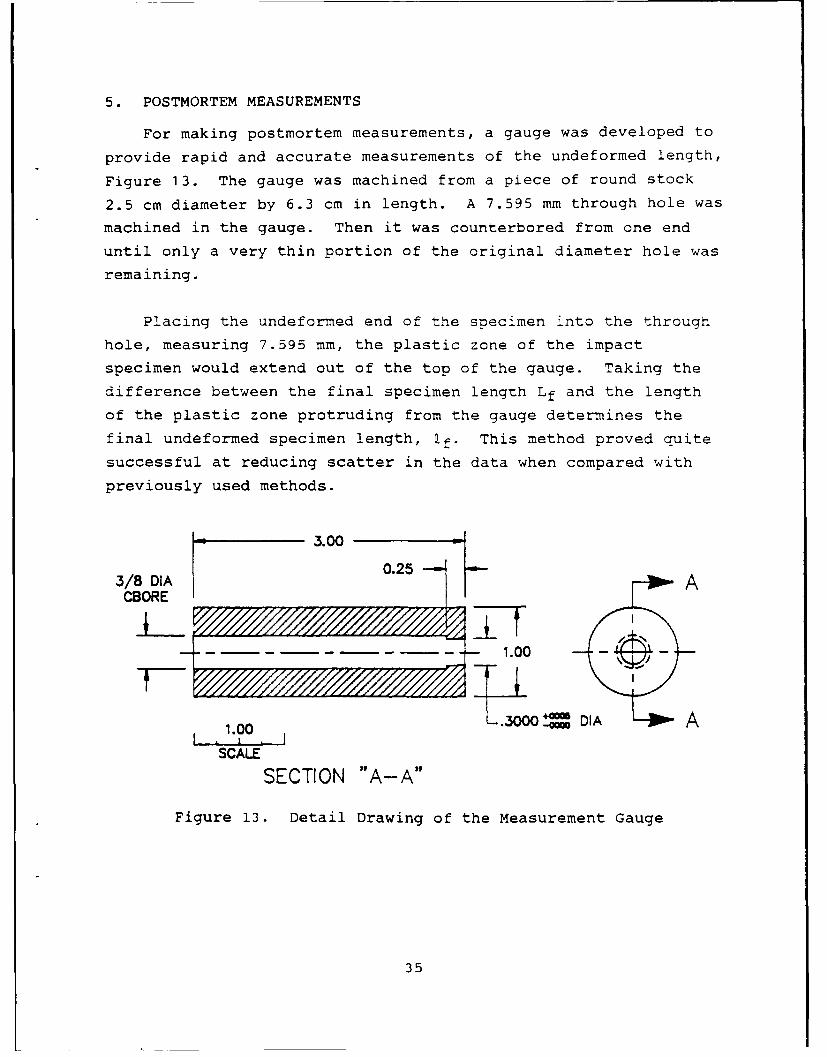
5. POSTMORTEM MEASUREMENTS
For making postmortem measurements, a gauge was developed to
provide rapid and accurate measurements of the undeformed length,
Figure 13. The gauge was machined from a piece of round stock
2.5 cm diameter by 6.3 cm in length. A 7.595 mm through hole was
machined in the gauge. Then it was counterbored from one end
until only a very thin portion of the original diameter hole was
remaining.
Placing the undeformed end of the specimen into the through
hole, measuring 7.595 mm, the plastic zone of the impact
specimen would extend out of the top of the gauge. Taking the
difference between the final specimen length Lf and the length
of the plastic zone protruding from the gauge determines the
final undeformed specimen length, If. This method proved quite
successful at reducing scatter in the data when compared with
previously used methods.
3.00
3/8 DIA 0.25ACBORE
- --1~ I
1.00 .3000 A
SCALE
SECTION "A- A"
Figure 13. Detail Drawing of the Measurement Gauge
35
SECTION IV
ANALYSIS OF TEST RESULTS
1. INTRODUCTION
The primary goal of the experimental work was to provide a
iaLa nase to us*- with various computer models. Information
contained in the data base was used to calculate the yield
stress and to construct graphs of the yield stress as a function
of various experimental parameters. In addition, a study was
made of the sensitivity of the computed yield stress to
perturbations in the experimental data. From this study an
estimate of the quantitative amount of error possible in the
calculations of the yield stress can be made. This report will
give evidence supporting the use of the a/p model, Reference 8,
for predicting the material behavior under impact conditions.
The test matrix was designed to generate data covering a
wide range of velocities, material types, and specimen aspect
ratios. The experimental data, along with results calculated
from the various analytical models, were organized by material
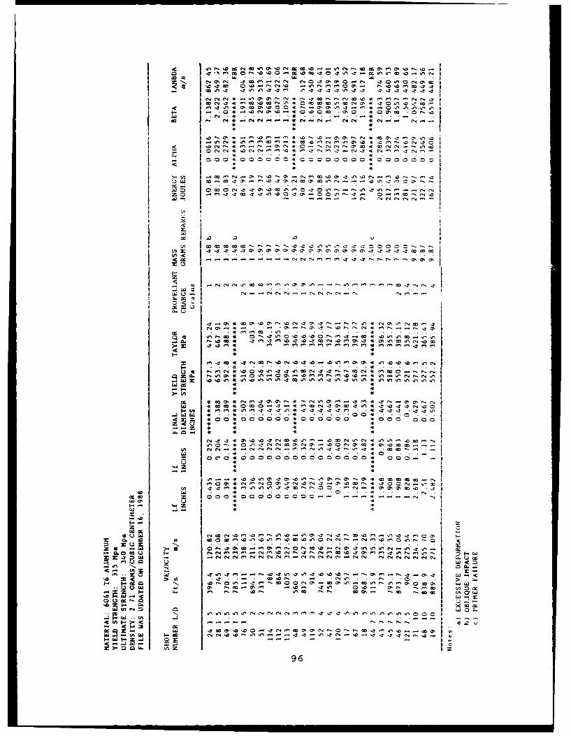
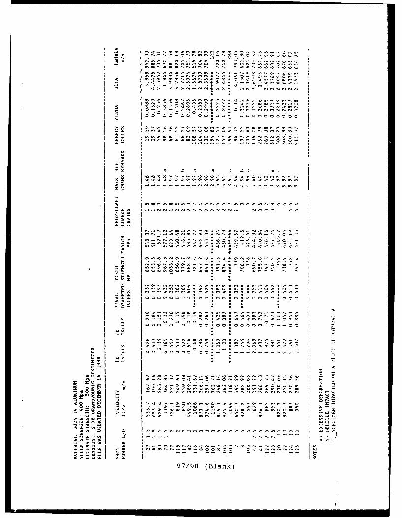
type and can be found in Appendix B.
The range of impact velocities used in this investigation
was 120 to 330 m/s. For a particular material, the upper
boundary for the impact velocity was limited by radial cracking.
For pure copper, the maximum impact velocity was approximately
200 m/s. The DPTE copper alloy had a maximum velocity of 160
m/s. For the aluminum alloys, the 2024-T4 material had a
maximum velocity of 290 m/s, while the 6061-T6 had a maximum
velocity of 330 m/s.
36
2. POSTMORTEM MEASUREMENT RELIABILITY
The reliability of the experimental measurements can be
judged by monitoring the trends in the data as a function of a
process variable. Figure 14 shows how the nondimensional forms
of the final length, Lf/L, and the final undeformed length,
If/ij, vcry with Lhe impact viocitý tor Jhe tour test materials.
These data show that the final length and undeformed length
decrease approximately linearly with increasing velocity of
impact.
After curve fitting the data by linear regression, a statis-
tical analysis, Table 3, reveals the level of uncertainty to be
found in the postmortem measurements. For the final length
measurement, the largest average deviation and maximum deviation
were 1.41 and 4.35 percent, respectively. A similar analysis
revealed a considerable amount of scatter was present in the data
for the final undeformed length. The largest average and maximum
deviations were 6.75 and 42.09 percent, respectively.
The primary source of scatter in the measurement of the
final undeformed length is from non-symmetric deformation.
Oblique impact with the target was often found to be the source
of such deformation. When a specimen impacts the target
obliquely, the plastic zone will extend further down one side of
the specimen than on the other. The measurement technique for
determining the final undeformed length used a gauge developed
with the premise that the specimen deformed in an axisymmetric
manner. Specimens that were visually identified as having
impacted obliquely were not measured.
37
z z
0
QI L- a . 0 o
* 6 0 0 9
41H0~ O41
CL 4)
Lac 0
aLLJ00 _
>' (A t
<00
900UAJ 0< 0
J -J
00
00 0 0D 0 00
p C)
38
TABLE 3. LINEAR REGRESSION AND STATISTICAL DATA
SLOPE Y.INTERCEPT AVERAGE % MAXIMUM %MATERIAL DATA (l/crns) (m/cm) DEVIATION DEVIATION
OFHC j/L vs V - 0.0020 1.124 1.41 4.35
OFHC ifiL vs V - Z.CuiA 0.644 6.75 42.39
DPTE Lf/L vs V - 0.0022 1.145 0.81 1.71
DPTE 11/L vs V - 0.0032 0S327 322 7.22
2024-T4 Lf/L vs V - 0.0008 1.088 0.80 2.48
2024-T4 If/L vs V - 0.0014 0.712 3.70 13.95
6061-T6 Lf/L vs V - 0.0012 1.140 0.83 2.796061-T6 If/L vs V - 0.0013 0.712 4.02 10.36
3. STATIC AND DYNAMIC STRENGTHS
The strength of the materials, at low strain rates, wasdetermined by quasi-static tensile tests. Specimens for the
test were machined from various sections of each of the rods.
The specifications for the fabrication of the tensile specimenscan be found in Appendix C. The tensile tests were conducted on
a screw-driven Instron machine at a crosshead displacement rateof 8.5 x 10⁻³ mm/s. Typical load versus time plots can be found
in Appendix D.
The data obtained from the impact tests was used in acomputer program which determines the dynamic yield stress of
the material. The program was designed to solve for the
nondimensional plastic wave speed, g, and the nondimensional
yield stress, a. The parameter A is determined by Equation
(41), page 19. The computer program uses an interval halving
technique to solve Equation (41) for the parameter A. The par-
ameter a is determined by Equation (37), page 18, and is directlycalculable once A has been found. Knowing a and p, the yield
39
stress and the plastic wave speed can be easily determined fromtheir definitions given following Equation (37), page 18.
The values of the yield stress from tensile test and thosecomputed by the a/p model are shown in Table 4. In general, the
dynamic yield stress is approximately 1.5 to 2 times the quasi-static value of the yield stress. This increase in the yieldstrength in the material corresponds to a change in the strain
rate of 7-8 orders of magnitude.
In Table 4, the yields stress values for the two coppermaterials were not reported. The response of the copper
TABLE 4. COMPARISON OF STATIC AND DYNAMIC YIELDSTRESS VALUES
QUASI-STATIC DYNAMIC(TENSILE TEST) (IMPACT TEST)
YIELD ULTIMATE YIELDMATERIAL STRESS STRESS STRESS
OFHC - 350 Mpa 550 Mpa
DPTE - 300 Mpa 520 Mpa
2024-T4 400 Mpa 500 Mpa 750-900 Mpa
6061-J6 315 Mpa 340 Mpa 550 Mpa
materials to loading was affected by the high dislocationdensity pre-existing in the material. This material condition
created a load versus time curve, Appendix D, in which the
stress level rose linearly to a maximum value and then
immediately decreased. The high dislocation density in thematerial effectively eliminated the work hardening region of the
stress versus strain curve.
4. SENSITIVITY ANALYSIS
An estimate of the error found in the computed value of theyield stress can be determined from a sensitivity analysis.
40
This analysis was conducted by estimating the level of accuracy
associated with each experimental measurement, e.g., the final
undeformed length. The value of the yield stress was
recalculated after the data were perturbed an amount equal to
the uncertainty in each measurement. A quantitative estimate of
the pzssitle crrcr is found by comparing the baseline value of
the yield stress with those found in the sensitivity analysis.
The measurements of specimen geometry, the final length, and
the final undeformed length were estimated tc be accurate to
within ±0.025 mm and ±0.076 mm, respectively. The velocity
measurements were considered accurate to within ±3 m/s. The
accuracy imposed on the velocity measurement system is taken
from an analysis of the uncertainty of data generated by the
pressure transducers. It was assumed fur this analysis that thewave forms recorded provided the optimum level of resolution and
the information was collaborated by the infrared detector and
the high speed photography techniques previously discussed.
Correlating the velocity data between the various measurement
systems provided an increased level of confidence in the
accuracy of the measurement. By choosing the results of a
particular impact test as a baseline, the effect of possible
inaccuracies in the experimental parameters on the computed
yield stress can be studied.
Table 5 shows a set of baseline values for two different
pure copper specimens with aspect ratios of 1.5 and 10. By
examining the data from specimens with different geometries, the
relative influence of possible inaccuracies can be considered.
Perturbed values of these parameters, according to the assumed
accuracy of the measurement, are shown in the columns headed with
a plus and a minus sign.
In Table 6, the dynamic yield stress values are given for
the baseline and from computations using the perturbed parameter
41
TABLE 5. EXPERIMENTAL TEST DATA
ASPECT RATIO
1.5 10
MEASUREMENT - BASELINE + - BASELINE +Lf 9.093 mm 9.119 mm 9.144 mm 60.528 mm 60.554 mm 60.579 mm
If 3.708 mm 3.785 mm 3.861 mm 27.000 mm 27.076 mm 27.153 mm
V 165.3 m/s 168.3 m/s 171.3 mis 163.0 m/s 166.0 m/s 169.0 m/s
values. In making the calculations only one of the three
measurements were varied from the baseline value. For example,in the first row, using a specimen with L/D of 1.5, the yield
stress was calculated using a value of the final length of
9.093 mm, 9.119 mm, and 9.144 mm; the baseline values were used
for the other two parameters, If and V. in the second and third
row of Table 6, the perturbed parameter was the undeformed length
and velocity, respectively. A quantitative estimate of the
uncertainty can be determined from a ratio of the difference
between the computed yield stresses found using the perturbed
experimental parameters to the baseline value. The percent
errors were 3.4, 2.0, and 7.2, for measurements of Lf, Qf, V,
respectively, for a specimen with an aspect ratio of 1.5. By
comparison, the second set of data produced percentage error
values of 0.6, 0.4, and 7.2, from measurements of Lf, If, and V,
respectively. The velocity measurement provided the greatest
source of uncertainty in both data sets. By comparison to the
velocity measurement, the deformee specimen geometry had little
influence on the overall uncertainty of the computed yield stress
value.
An argument could be made that additional combinations of
the various parameters would produce a larger deviation from the
baseline value. Note in Table 6 that a reduction of the geometry
parameters, Lf and Qf, had an opposite effect on the computed
yield stress value. Reducing the final undeformed length, If,
42
increases the stress value, while a reduction in the final
length, Lf, decreases the calculated stress. It was considered
that the actual uncertainties in postmortem measurements would
be small, or possibly cancel one another, by comparison to those
found in the velocity measurement. Therefore, the yield stress
values reported in Table 6 as baseline values and those given in
5 ARUCO IRON -- 506 SOFT DURAL 8-15 197 LEAD -- 2.88 COPPER -- 15.5
ooo ThE SMAL. FIGURE.S IN THE DIAGRAM SHOW "THE STRIKING VaLOaTY EMPLOYED.
Figure 16. Mondimensional Form of the Undeformed Final
Length as a Function of the NondimensionalFinal Length Parameter
47
TAYLOR IMPACT EXPERIMENTNA vs UA
0.9-
0.7-SOF'HC
0.6- + OPTE
J 2024-T40.5 x 6061-T6 x 0
0.4 0
0.3-
x o0.2-
0
0.1-
0-0 0.2 0.4 0.6 0U8
U/A.
Figure 17a. Ballistic Geometry Data, in NondimensionalForm, for the Current Investigation
48
TAYLOR IMPACT EXPERIMENTNIL/ vs !A.
0.5
0.481 1.5
0.46- 2
0.44- 7.5
0.42-1.5
0.4,- 2024-T4
0.38-
0.36 104
0.34 A -1
0.32- Tj 3.2
O.3- 43 2
0.n -
0.24
0.22
0.210.7 0.74 0.78 0.2 0.86 0.9 0,94 0.6
U/L
Figure 17b. Ballistic Geometry Data, in NondimensionalForm, for 2024-T4 Specimens
49
6. MUSHROOM GROWTH
The measurement of the final diameter of the specimen at the
target/specimen interface indicates that the mushroom growth is
correlated with the available energy on impact, Figure 18. A
comparison between short and long specimens shows that the final
diameter is proportionally greater for longer specimens,
depending on the mass increase, for equal impact velocities.
These results indicate that the final diameter of the mushroom
is dependent on the strength of the material and the kinetic
energy at impact.
50
>>
0
4-)
Q -4- 0,-
-E 0 .- UnI
0.- M~ 4.
L.LJ C ....a_ C 0i
L > Ilaa a C3 L
+ Q
-. - -
< r-4
0 70
ýn0 2n ,
-< FL. ' ! _L.] A I . b l -:
5-1
7. HIGH SPEED PHOTOGRAPHY
The Cordon framing camera was used to generate a photographic
record of a particular impact test (UK-145). The camera was
operated at a framing rate of 300,000 frames per second. At this
rate, the resolution of the photographic data was 3.33 As. The
impact event was photographed using a shadowgraph technique.
Measurements taken directly from the photographs provided data on
the mushroom growth and the rear end position both as a function
of time.
The data obtained on the mushroom growth rate, Figure 19,
indicates the magnitude of the strain rates seen at the
TAYLOR IMPACT EXPERIMENT0.00 UK - 145
MUSHROOM STRAIN vs TIME
Z -0.20
or-
(i-
Qý0
-0.60
[D
-0.80
- 1.00 ... ......0.00 20.00 40.00 60.00 80.00
TIME, (js)
Figure 19. Strain at the Target/Specimen Interfaceas a Function of Time
52
specimen/target interface. The photographs show that the bulk ofthe mushroom growth process occurs within the first few microse-
conds and is completed by-40 As after impact. The slope of thecurve in Figure 19 gives a strain rate of 7.5 x 10 4 /s during the
first 7 Ms.
The data on the position of the rear end of the specimen asa function of time shows that it took 120 As to bring the
specimen to rest, Figure 20. The velocity of the rear end issimply the slope of the curve. The data show that the initialvelocity, 190 m/s, did not change until approximately 45 As
after impact.
0.80 Taylor Impact ExperimentUK-145
Relative Position of the Undeformed End versus Time
c--C 0.60
Linear Curve FitX - - 0.00744t + 0.6794" *X Where:SX
Figure 20. Position of the Undeformed End of theSpecimen as a Function of Time
53
The analytical models which attempt to describe the physical
process assume that the plastic front moves at a uniform velocity
throughout the event. The calculated plastic wave speed from the
a/g model should be considered to be an average value. For the
particular test that was photographed with the framing camera, a
comparison of the plastic wave speed calculated from the model
can be made with experimental results. Knowing the duration of
the event and the distance traveled by the plastic wave, a velo-
city was determined. For test UK-145, the model computed a value
of 202 m/s for the parameter, >. From the photographs, the plas-
tic wave speed is calculated to be 212 m/s, which is in good
agreement with the value predicted by the model.
54
SECTION V
MICROSTRUCTURE
1. INTRODUCTION
The materials considered for this investigation varied
widely in their microstructural features. The differences in
deformed geometries reflect how the microstructure of each
material influenced the mechanisms for plastic deformation. The
principal aspect of this study is how the basic microstructure
affects the way the material absorbs the energy of impact.
Macroscopically, the features of a deformed specimen were
similar for all of the materials. The grains on the axis near
the anvil, which are subjected to high compressive loads, are
extensively deformed. The longitudinal compressive strains
impart radial motion to the deforming body to produce the
characteristic mushroomed profile. The extent of the deforma-
tion process is governed by various aspects of the microstruc-
ture, which is controlled by the thermo-mechanical history of
the material and its chemical composition.
The structures found in the materials used for this
investigation were of three types: single phase, multiphase
containing inclusion particles, and multiphase containing
inclusions and coherent precipitates. The first of these
structures is found in OFHC copper (99.99 Cu). The second type
is found in DPTE copper and in 6061-T6 aluminum. The last typeis found in 2024-T4 aluminum. The constituents found in each of
the materials are given in Table 7. The heat treatments
specified for the aluminum materials correspond to a solution
anneal followed by artificial aging, for 6061, and natural
aging, for 2024. Some specimens of OFHC copper were annealedfor 1 hour at 600 0 C in a vacuum. The nomenclature annealed
copper and half hard copper will henceforth be used to denote
55
the CFHC copper in the annealed and as-received conditions,
respectively.
All of the materials were examined by optical microscopy
both before and after impact. The OFHC coppers were more
extensively studied. In addition to optical examination, X-ray
diffraction and transmission electron microscopy (TEM)
techniques were used to study the microstructure and the effect
of high strain rate deformation.
56
I 0
z LU LL
0 On L o m
<. -j < - - -9 -
= < - < -- I
z cc
CD 1 8 CD
I- - -*)
.- -- 1
uu
0Ea
I3- CD OOD~J (
C!
577
2. DPTE COPPER
The DPTE copper material is a copper/tellurium alloy. Tellu-
rium is added as a solution strengthening element in small
amounts. A small concentration of phosphorous is added as a
deoxidizer. The phosphorous removes oxygen from the copper
matrix by forming oxide inclusion particles. During hot rolling
of the material these inclusions are broken up and elongated in
the rolling direction. The final structure after cold working
the material shows a fine grain structure with an extensive
number of stringers elongated parallel to the rod axis, Figure
21.
Zoo"
3. 6A
t _0.2mm
Figure 21. Optical Micrograph Showing the Microstructureof OPTE Copper
3. 6061-T6 ALUMINUM
The 6061-T6 is a ternary aluminum alloy containing small
concentrations of silicon and magnesium. Age hardening will
produce a matrix of aluminum with :aagnesium in solution and
precipitates of Mg2 Si. These precipitate particles will be
58
spherical in shape, Figure 22, and will be incoherent with the
matrix. In commercial grades, inclusions of aluminum oxides and
iron/silicon compounds will be found that are not affected by
subsequent heat treatment. The size of the misfit between
lattice types, the aluminum matrix and the precipitate, produces
a small internal strain field surrounding each precipitate. This
small strain field produces little disruption to the motion of
dislocation which occurs under an applied load.
Figure 22. Optical Micrograph Showing the Microstructureof 6061-T6 Aluminum
The shape of the precipitate particles reduces the number of
potential sites for localized stress concentration. In turn,
preventing the localized buildup of stress inhibits crack
nucleation and growth. This microstructure in the 6061-T6 alloy
provides a relatively low yield strength, but gives it a high
toughness, i.e., the ability to absorb energy before fracture.
59
4. 2024-T4 ALUMINUM
The 2024-T4 is a ternary aluminum alloy containing copper
and magnesium. Allowing the material to naturally age after
solution anneal provides the opportunity for coherent AI 2 Cu
precipitates to form on (001) habit planes. In addition,
magnesium and aluminum oxides form inclusion particles in the
matrix, Figure 23. The formation of the coherent AI 2 Cu
precipitates, which have a large misfit with the matrix,
prevents the easy motion of dislocations on the slip planes.
Therefore, the material shows increased strength by comparison
to the 6061-T6 alloy, see Table 1.
4e
.... . _.• .,: • 0.2rnrn
Figure 23. Optical Micrograph Showing the Microstructureof 2024-T4 Aluminum
5. OFHC COPPER
Optical examination of the half hard OFHC copper material
shows that slip is the primary mode of accommodating the
deformation introduced by drawing, Figure 24. TEM thin foils of
60
the material showed an extensive substructure containing an
inhomogeneous distribution of dislocations, Figure 25. The
parallel bands seen in Figure 25 indicate that deformation twins
were formed during the processing of the material.
Figure 24. Optical Micrograph of the Microstructure ofHalf Hard OFHC Copper
Reports by Ahlborn and Wassermann, Reference 11, and
Wassermann, Reference 12, cite evidence that the following
conditions give an increased incidence of mechanical twinning in
drawn copper wire:
a. lowering the deformation temperature, Reference 13,
b. increasing the amount of deformation,
c. lowering the stacking fault energy by alloying.
The as received material was in a half-hard condition, which
means that following the final anneal there was a reduction in
cross sectional area of 30 to 60 percent. This amount of
straining satisfies condition b, rqported above, and is
confirmed by the TEM observations in Figure 25.
61
Ji
Figure 25. TEM Micrograph of Half Hard OFHC Copper
Figure 26. Optical Micrograph of the Microstructure ofAnnealed OFHC copper
62
Pole figures were generated to determine the textures of the
half-hard and annealed OFHC copper materials. Because of the
drawing operation, the texture in the half hard material was
found to be oriented parallel to the rod axis and was a
superposition of (111) and (001) fiber textures. The annealed
material had a random grain orientation with an approximate
grain size of 40 um. Compare Figures 24 (half hard) and 26
(annealed).
6. MICROSTRUCTURE RESULTING FROM IMPACT
With different metallurgical histories, two copper specimens
which impact the target at similar velocities accommodated the
energy in significantly different ways. Examination of the
post-impact geometries reveal how the microstructure influenced
the deformation, Figure 27. The specimen on the left was
deformed in the half-hard condition. The specimen on the
right was deformed in the annealed condition. The three post-
mortem measurements of the geometry that were visibly influenced
by the microstructural differences are the final mushroom
diameter, the final length, and the extent of the plastic
deformation in the specimen.
The half-hard copper specimen had a much greater change in
diameter. The annealed specimen had a greater reduction in final
length and was traversed entirely by the plastic wave in the
material. From these observations, it is quite evident that the
dislocation density in the material had a significant role in
how the impact energy was absorbed.
Following impact, both types of copper specimens were
sectioned parallel to the rod axis. An optical examination was
conducted near the mushroom face close to the original rod axis,
Figures 28 and 29. The large compressive loads are evident by
the collapse of the grains. After impact, the grains of the
annealed material run parallel to the target face, Figure 28.
63
Figure 27. Impact Specimens of OFHC Copper
In contrast, the half-hard copper specimen contains small,
randomly oriented grains, Figure 29. These grains indicate that
the mechanical history of the material created a condition
suitable for recrystallization to occur as a result of impact.
To confirm this observation, back reflected Laue patterns
were generated from both types of impact specimens. The x-ray
beam was positioned to strike near the same location as shown in
the optical micrographs. Results for the annealed impact
specimens showed two diffuse rings. The impact specimen used in
the half-hard condition showed two rings made up of numerous
intense spots. These bright spots occur because of the increase
64
Figure 28. Optical Micrograph Showing the Microstructureof Annealed OFHC Copper After Impact
0.4 mmFigure 29. Optical Micrograph Showing the Microstructure
of Half Hard OFHC Copper Specimen After Impact
65
;n size of the coherently diffracting domain created by the
recrystallization process.
The high dislocation density in the half hard material had a
significant effect on the behavior in both impact tests and
tensile tests. In tensile tests, performed for quasi-static
characterization of the material, the high dislocation density
effectively eliminated the strain hardening region of the load
versus time plot, Appendix D. The load increased linearly until
localized plastic deformation occurred so that the yield and
ultimate strengths of the material coalesced into one point.
During the deformation on impact, the dislocation density
influenced how the material absorbed the energy. As previously
mentioned, this observation is evident by the macroscopic
features of the post-impact geometry, Figure 27. The
post-impact geometries suggests that recrystallization occu:red
in the half-hard material because the heat generated by plastic
work was more intense. In addition, the increase in stored
energy in the material caused by cold working reduces the amount
of energy required for recrystallization. The temperature for
the recrystallization of copper is 225 0 C.
After impact, TEM thin foils were made from both types of
copper materials. The half-hard material showed a high
incidence in the number of deformation twins, Figure 30. Since
the material had contained twins initially, the source of the
twins could have been either the impact event or the processing
of the original rod stock. However, deformation twins were also
found in the specimens of annealed material. These could only
have been produced by impact.
TEM replicas were taken from the surface of the sectioned
half-hard impact specimen. Examination of these replicas
revealed an orientation relationship that identified the
formation of a twin with the impact event, Figure 31. Previcus
investigators, Reference 14, identified similar artifacts as
66
compression twins formed in shock loaded single crystals of pure
copper. (See Figure 14, in Reference 14.)
Figure 30. TEM Micrograph Showing Deformation Twins in OFHCCopper
Brilhart and coworkers, Reference 15, investigated theformation of deformation twins in polycrystalline pure copper byshock loading the material using flyer plate experiments. Inthese experiments the pressures responsible for the formation ofdeformation twins were on the order of 7.5 GPa.
The observation of deformation twins in pure copper Taylortest specimens suggests the level of pressure in the material on
impact. The pressure on contact between the specimen and thetarget was estimated by a model constructed using Hugoniot
relationships, as detailed in Appendix E. From this analysis thepressure at the moment of impact, in a copper specimen strikinga steel anvil at an initial velocity of 200 m/s, is 3.9 GPa.
This estimated pressure is nearly an order of magnitude abovethe dynamic yield stress of the material.
67
Figure 31. Photo-Micrograph of a TEM Replica Showing aShock Formed Twin in Half-Hard OFHC Copper AfterImpact
The mechanical behavior of copper was significantly affected
by increasing the impurity content. Increasing impurity content
reduced ductility. In static tests, the percent elongation, or
strain, at which failure occurred was lower in the DPTE copper
than in the OFHC copper.
In dynamic tests, the data showed that the DPTE copper
failed, by fracture on the periphery of the mushroom diameter, at
impact velocities greater than 160 m/s. Failure of the impact
specimen resulted from the large circumferential strains produced
by the radial motion of the deforming material. Among DPTE
copper specimens which had not cracked radially, the largest
mushroom diameter measured was 20 percent less than for OFHC
copper specimens.
The type of fracture found in the DPTE copper material was
indicative of the microstructure. The high level of impurities
68
provided numerous locations within the material for the localized
build up of stress. The ability of t e matrix to accommodate the
strain was reduced by the addition of tellurium. Numerous sites
for stress concentrations, and reduced matrix ductility, produced
a material that fractured at relatively low strain levels. The
mode of failure was by brittle fracture as indicated by the
grainy texture of the fracture surfaces.
By comparison, the OFHC copper specimens failed in a ductile
manner. Close observation of the mushroom periphery in Figure
27 shows the early stages of crack growth. Note the region of
deformation which surrounds each crack and is typical of ductile
failure.
The inclusions, or stringers, in the DPTE copper material
provide a unique way of examining the results of deformation
within the specimen. During the original processing of the rod
stock the oxide inclusions were broken and elongated in a
direction parallel with the axis of the rod. After impact,
examination of the new orientation of the stringers and grain
boundaries within the material revealed certain aspects about the
deformation resulting from impact. During impact, the grains
compress in the direction of the specimen axis, while expanding
radially. Comparison of the grain boundaries before and after
impact, Figures 21 and 32, reveals that the grains at the axis
now run parallel to the anvil. To accommodate the large
compressive strains, the free boundary moves radially outward.
In the region nearest the free surface stringers that are
initially oriented axially reorient as the free surface changes
shape, Figure 33. Therefore, the shortening of these stringers
is less than those near the specimen axis, allowing these
inclusion stringers to retain their basic shape. The radial
expansion that has occurred in the material is depicted by the
new alignment of the stringers. Compare Figures 21, 32, and 33.
69
• 0.2 mm
Figure 32. Optical Micrograph Showing the Microstructureof DPTE Copper After Impact
0.2 mm
Figure 33. Optical Micrograph Showing the Microstructureof DPTE Copper, After Impact, Near the FreeBoundary Surface
70
The two aluminum materials responded to the deformation in a
manner consistent with their respective microstructures. The
grains on the axis of the 6061-T6 aluminum alloy readily
deformed, Figure 34. However, the 2024-T4 material, Figure 35,
resisted the large amount of deformation seen in the 6061-T6
alloy. This is evidence of what effect second phase particles
have on the dislocations as opposed to incoherent intermetallic
particles. The finely dispersed sacond phase precipitates in
the 2024-T4 alloy act as pegs for the dislocations, which
attempt to move along the slip planes in response to the applied
stress. It can be seen in Figure 35 that slip bands have been
formed in certain grains. These grains have crystallographic
orientation which maximizes the shear stress found on the slip
plane. Once the A1 2 Cu precipate is sheared, additional
h 0.2 mm
Figure 34. Optical Micrograph Showing the Microstructurein 6061-T6 Aluminum After Impact
dislocations readily move through the material. The inclusion
particles of 6061-T6 aluminum being larger in size and spaced
further apart than the precipitates in 2024-T4 provides little
resistance to the motion of dislocations.
71
The energy which can be absorbed by a material is defined by
its toughness and is indicated in the Taylor anvil test by the
strain to failure and the extent of the plastic deformation.
The 2024-T4 alloy has high strength, but relatively low tough-
ness, compared with the 6061-T6 alloy. The geometry of the
inclusion particles found in 2024-T4 are very irregular, Figure
23. This shape produces localized stress concentrations which
4. G.R. Johnson and W. Cook, Proceedings of the SeventhInternational Symposium on Ballistics, The Hague, TheNetherlands, pp. 541 (1983).
5. F.J. Zerilli and R.W. Armstrong, J. Appl. Phys. S1,1825 (1987).
6. N. Cristescu, Dynamic Plasticity, (John Wiley andSons, Inc. New York, 1967).
7. J.B. Hawkyard, Int. J. Mech. Sci. 11, 313 (1969).
8. S.E. Jones, P.P. Gillis, and J.C. Foster, Jr. J. Appl.Phys. 61, 499 (1987).
9. A.C. Whiffin, Proc. R. Soc. London, Series A, 194, 300(1948).
10. M.L. Wilkins and M.W. Guinan, J. Appl. Phys. 44, 1200(1973).
11. H. Ahlborn and G. Wassermann, Z. Metallk. 54, 1(1962).
12. G. Wassermann, Z. Metallk. 54 (1963).
13. T.H. Blewitt, R.R. Coltman, and J.K. Redman, J. Appl.Physics, 28, 651 (1957).
14. R.J. De Angelis, and J.B. Cohen, Proceedings of theAIME - IMD Conference on Deformation Twinning (Gordonand Breach Publishers, New York, 1964) p. 430.
15. D.C. Brillhart, R.J. De Angelis, A.G. Preban, J.B.Cohen, and P. Gordon, Trans. AIME, 239, 836 (1967).
16. P. Ludwik, Elemente der Technologischen Mechanick,(Springer, Berlin, 1909), p 32.
17. P.S. Follansbee and U.F. Kocks, Acta Metall. 36, 81(1988).
83
BIBLIOGRAPHY
S.E. Axter, W.B. Jones, and D.H. Polonis, Metallography,8, 425 (1975).
J.D. Campbell, Dynamic Plasticity of Metals, (Udine, NewYork, 1970).
W.E. Carrington and M.L.V. Gayler, Proc. R. Soc. London,
Series A, 194, 323 (1948).
R.J. Clifton, J. Appl. Mech. 50, 941 (1983).
P. Gordon. R. Karpp, S. Sanday, M. Schwartz, J. Appl,Phys. 48, 172 (1977).
H.A. Grebe, H.R. Pak, and M.A. Meyers, Metal. Trans. A,10A, 569 (1979).
J.B. Hawkyard, D. Eaton, and W. Johnson, int. J. Zecn.Sci. 10, 929 (1968).
I.M. Hutchings and T.J. O'Brian, Int. J. Mech. Sci. 23,255 (1981).
W.B. Jones and H.I. Dawson, Metallurgical Effects at HighStrain Rates, (Plenum, London, 1973) p. 443.
E.H. Lee and S.J. Tupper, J. Appl. Mech. 21, 63 (1954).
G. Regazzoni, U.F. Kocks, and P.S. Fcllansbee, ActaMetall. 35, 2865 (1987).
J.S. Rhinehart and J. Pearson, Behavior of Metals UnderImpulsive Loads, (ASM, Cleveland, 1954).
A.K. Sengupta, G.J. Wigglesworth, S.K. Ghosh, W. Johnson,
and S.R. Reid, J. Mech. Eng. Sci. 24, 31 (1982).
C.S. Smith, Trans. AIME, 214, 574 (1958).
T. von Karmen and P. Duwez, J. Appl.Phys. 21, 987,(1958).
84
.PPENDIX A
TEST PROCEDURES
85/86 (Blank)
APPENDIX A
TEST PROCEDURES
2) Remove target housing cover. Clean debris, if any,
off of the plexiglass windows.
2) Remove and clean pressure transducers, if necessary.
3) Prior to mounting the pressure transducers in themuzzle, apply a thin layer of silicon grease over thepiezo-crystal surface to act as a damper on the pressurewave.
4) Check the voltage output from the infrared deteczzrcircuit. A low voltage state indicates debris iscovering the detector lens and must be removed.
5) Clean the infrared detector lens, if necessary.
6) Rotate the target, if necessary, and position thefiducial (magnet) on the target face one-half inch abovethe point of impact.
7) Bore sight the high speed camera, or the framingcamera, if necessary. The camera lens should be as nearparallel to the target face as possible.
8) If high speed photography is to be used, load thecamera with film.
9) Set the desired standoff distance between the muzzleand the anvil. Tiqhten the bolts on the v-block mountsto secure the launch tube.
10) Replace the target housing cover.
11) Weigh specimen. (grains)
12) Measure specimen diameter. (inches)
13) Weigh propellant charge. (grains)
14) Load the measured quantity of propellant into acartridge.
15) Insert a ball of cotton into the cartridge case andpack against the propellant.
16) Obtain the safe/arm panel keys.
17) Insert a specimen, followed by an obturator, intothe breech end of the launch tube.
87
18) Position the specimen and obturator at the correctdepth in the launch tube using depth measurement gauge.
19) Insert the cartridge case behind the specimen andobturator. Screw the breech cap on the barrel until thescribed marks are aligned.
20) Attach the firing solenoid to the breech.
21) Remove shunting connector from the firing line andconnect the firing line to the firing solenoid.
22) Insert the firing pin to the prescribed depth intothe firing solenoid.
23) Remove shorting plug from firing line and connectfiring line to firing power supply output panel.
24) Arm the firing power supply circuit.
25) Arm the firing signal control panel.
26) After arming the firing signal control panel, moni-tor the cnarge level of the firing power supply untilthe predetermined voltage level is reached. Once theappropriate energy level is reached the firing count-down can begin.
27) At t minus 20 seconds, the multitrack signalrecorder is turned on.
28) At t minus 5 seconds, when using the high speedmovie camera, the photographic light is turned on.
29) At t minus 3 seconds, the high speed camera isturned on.
30) At t equal to 0, the firing signal is sent to thehigh speed movie camera and to the firing solenoid.
31) Disarm the control panel.
32) Disarm the firing circuit.
33) Remove the firing circuit wire connected to thefiring solenoid.
34) Unscrew the breech end cap and extract the spentcartridge case.
35) Clean debris from the launch tube bore with a guncleaning rod tool.
88
36) Remove target cover and retrieve the impactspecimen and obturator. Discard obturator.
37) Remove high speed movie film, or framing camerafilm, if necessary.
38) Measured from the oscilloscope, record the durationof time between the leading edge of the pressure trans-ducer signals.
39) Obtain a strip chart output of the transducer sig-nals from the multichannel recorder.
40) Using the strip chart output, digitize the referencesignal (frequency = 100 khz). Digitize the leading edgeof the pressure transducer signals.
41) Obtain a print out of the digitized data convertedto specimen velocity.
42) Measure the final diameter of the mushroomed portionof the specimen.
43) Measure the final length of the specimen.
44) Measure the undeformed length of the specimen.
89/90 (Blank)
APPENDIX B
DATA FILES
91/92 (Blank)
f ~ ~ ~ a e0 10 40 10 a0 go w~ 1 0( ~NN*NNN ~ %0
In wS '.0 -. N 140 m . In' % 'T0 m% 0% -0 0 w 0 K
ama lw 0m 1 0 -K d K7 c'*Cý1 I , N 00 go 0 K 0 K -. 0mC) 0o 0 K1(7 -
CN4 .1 10 N4 T~~~O w In -0 w ~K - N J - '
0.0 '4 -0 ' .N . c *
W,~~N '.N In* y'., c.. 0, C 0'a K
z0 .0 - - - -
vi61 ý I w
al In 0%I w
I ~~~0 o 00.'.
eN '-oa l Y
F- m
-- ~ ~ ~ ~ C N..-NN N 4 N N l .
zW I"mII If nn
I I 0'S '0NN 0 ' N.0'0%KN~~N 4'-.4'0%4'i'
I1 10 '
I 0 N'0%~'N~'.'.%'~N 0.0.0% 0 '00'~~''N''
I -~~ K '0~0%K 0~-0'r'N'0r,0''.
I > K N~*N ~'*COCO..
0 ~ ~ ~ ~ ~ 1 4 M C4~NKN'~'''0'
Q>Q CK . . K
do '. o e4f4 (' r4 V4'O 0KK K1 ~ -O
0 4 CN 4 C 4 - 4 C4 -- C.4 ''. ..-. '/.~
Me Q0'N 0' N0'N 4'
K (A K
LIS W 0. 0% 0 N .0 cy a. 4. 0 0 '0't.'0'0% '
C-' f.4 'aNN0'. .A 10 KN-N4 K ~ '/ 00
A 4~~'.'44'4~ .0'0~NN''0K0 0%'0 NL)
... .C ... .K ....3
C4 C4Cld C C4 4 C4 4 el
m - C'4 0 ' -. 0% .0 42 A 'Im ' C4 C- (4 w In m - 4ý &% (
00 -~ 'o ". ~ ~ '0
.4,0 o Co'-00 - 0, w en car. . . ..f .N .'. .' 0 . .a ,' 5.
C4 IT1C C4 m4 In
I1 0%( cc I
I-0 w lI ,1 'w9
0 IntA g go'D a 'a C4 P% y, (, (,(7
6A I^" VIco
'o 000 r6000 0
"" a104
La4 v UC ft a C .4 ~ 4' -747 4' C4 -CI
" 0.- u 0
24
-~4 --
40594
tA ~ ~ ~ ~ -40 " C4 "4 'T N 0 0 m V 0 ' as N- (7 r 4 n'7-0% -O ~ 'N , 4 ID 7 In ý ~-, 0 0 w -C0 -t w m
In m' In I0ITr
9 - N 0 'n '0 N '?ý ' r0 -0 C4' ~~' In en a In - m" ca Q0'C - - 00 a, 4'N-1U ' ~ ~ 'N0 N0 - '~ 0 In N~
rq CC Ln~4 ' m'4 Inf~ M %I4 0 C N a,A~~* 4:ý44' ~ . - - -
2' C4 M- - ."- - -I1
I4 C44 4' 4'U Z441 M 00 In
I I)
A Z In wII, C I - 7 1
I" C" m 11.4 10/~'4 -'ýt4 9 A A. " lýl
aIn 0'0' 4 '0110' N V In
-1 .c 4.1 - 4 - 41 V)44
I '4 'U 4 * C1 *' 7 0 k0 k Nt .09 41 -' 11 'A W0 w 49 4' 4' 4K A1 . -4
=: ** -kA .9 4' 4'A * 4' 4'4
*AA f -k AC 4'''0'' 4N41 IL 04'444'0N'' 4 it-K"A W I 04' .9 IN4 N 4' 4'444 4' It '4 'U44 '' ' ' 4