Taylor Polynomials Suppose you buy bonds at 90% of their face value. When you cash them in later at their full face value, what percentage profit will you make? The answer is not 10%. In fact, since you will get $1 for each $0.90 you invest, you get back 1 0.90 ≈ $1.11 for each dollar that you invest, giving you an 11% profit. Now think about this problem in another way. You are being offered a discount of x (in this case, x = 0.10). To find your profit you need to compute f ( x ) = 1 1 − x − 1. We would like to find an easier-to-compute approximation to f ( x ), to see why f (0.10) ≈ 0.11, and to see quickly what would happen for other discount rates. In fact, we shall see very soon that a good approximation is f ( x ) ≈ x + x 2 , if x is close to 0. When x = 0.10, this gives f (0.10) ≈ 0.10 + 0.01 = 0.11. What we are claiming then is that f ( x ) can be approximated by a polynomial. This is nice because polynomials are among the easiest functions to compute and manipulate. The more general question behind all of this is: How can any function f(x) be approximated (for values of x close to some number a) by a polynomial? One very useful answer is given by the following theorem. Its proof is easy from the column method of integration by parts, and we shall give this proof at the end of the section. Taylor’s Theorem with Remainder If f ( x ) is ( n + 1)-times differentiable, then f ( x ) = f ( a) + f ( a)( x − a) + f ( a)( x − a) 2 2! + f ( a)( x − a) 3 3! +···+ f (n) ( a)( x − a) n n! + R n where R n = x a f (n+1) ( t )( x − t ) n n! dt. Here, as usual, n! = n( n − 1)( n − 2) ··· 2 · 1 is called n factorial. 1
Transcript
Taylor PolynomialsSuppose you buy bonds at 90% of their face value. When you cash them in later at theirfull face value, what percentage profit will you make? The answer is not 10%. In fact,since you will get $1 for each $0.90 you invest, you get back
1
0.90≈ $1.11
for each dollar that you invest, giving you an 11% profit.Now think about this problem in another way. You are being offered a discount of x
(in this case, x = 0.10). To find your profit you need to compute
f (x) = 1
1 − x− 1.
We would like to find an easier-to-compute approximation to f (x), to see why f (0.10)≈ 0.11, and to see quickly what would happen for other discount rates. In fact, we shallsee very soon that a good approximation is
f (x) ≈ x + x2 ,
if x is close to 0. When x = 0.10, this gives
f (0.10) ≈ 0.10 + 0.01 = 0.11.
What we are claiming then is that f (x) can be approximated by a polynomial. This isnice because polynomials are among the easiest functions to compute and manipulate.The more general question behind all of this is:
How can any function f(x) be approximated (for values of x close to some number a)by a polynomial?
One very useful answer is given by the following theorem. Its proof is easy from thecolumn method of integration by parts, and we shall give this proof at the end of thesection.
Taylor’s Theorem with Remainder
If f (x) is (n + 1)-times differentiable, then
f (x) = f (a) + f ′(a)(x − a) + f ′′(a)(x − a)2
2!
+ f ′′′(a)(x − a)3
3!+ · · · + f (n)(a)(x − a)n
n!+ Rn
where
Rn =∫ x
a
f (n+1)(t)(x − t)n
n!dt.
Here, as usual, n! = n(n − 1)(n − 2) · · · 2 · 1 is called n factorial.
1
The polynomial
T (x) = f (a) + f ′(a)(x − a) + f ′′(a)(x − a)2
2!
+ f ′′′(a)(x − a)3
3!+ · · · + f (n)(a)(x − a)n
n!
is called the nth Taylor polynomial of f around a, or the nth Taylor expansion of f around a.1 The last term, Rn, is called the remainder, or error term; it allows usto estimate how well the Taylor polynomial approximates the function f.
It often happens that the remainder Rn approaches zero as n gets large. When Rn issmall, f (x) is approximately equal to its nth Taylor sum;
f (x) ≈ f (a) + f ′(a)(x − a) + f ′′(a)(x − a)2
2!
�f ′′′(a)(x − a)3
3!+ · · · + f (n)(a)(x − a)n
n!
For this reason we often call the Taylor polynomial the Taylor approximation ofdegree n. The larger n is, the better the approximation.
EXAMPLE 1 Taylor Polynomial
Expand f (x) = 1
1 − x− 1 around a = 0, to get linear, quadratic, and cubic approxima-
tions.
Solution We will use the formula for the nth Taylor polynomial with a = 0, forn = 1, 2, and 3. Thus, we need to calculate f (0), f ′(0), f ′′(0), and f ′′′(0). Let us listf (x) and these derivatives, evaluating at a = 0 each time.
f (x) = 1
1 − x− 1 so f (0) = 0
f ′(x) = 1
(1 − x)2so f ′(0) = 1
f ′′(x) = 2
(1 − x)3so f ′′(0) = 2
f ′′′(x) = 6
(1 − x)4so f ′′(0) = 6
We can now write the approximations one at a time.
Degree 1 approximation: f (x) ≈ f (a) + f ′(a)(x − a)Substituting, we get:
1
1 − x− 1 ≈ 0 + (1)x = x
So, the linear approximation to f (x) is the polynomial x.
2 Taylor Polynomials
1 When a = 0, this is also called the Maclaurin polynomial.
Degree 2 approximation: f (x) ≈ f (a) + f ′(a)(x − a) + f ′′(a)(x − a)2
2!Substituting, we get:
1
1 − x− 1 ≈ 0 + (1)x + 2x2
2!= x + x2 .
Thus, the quadratic approximation to f (x) is the polynomial x + x2.
Degree 3 approximation: f (x) ≈ f (a) � f ′(a)(x − a) �f ′′(a)(x − a)2
2!�
f ′′′(a)(x − a)3
3!Substituting, we get:
1
1 − x− 1 ≈ 0 + (1)x + 2x2
2!+ 6x3
3!= x + x2 + x3
Thus, the cubic approximation to f (x) is the polynomial x + x2 + x3.
Before we go on... Looking at the answers to Example 1, you probably suspect—correctly—that the fourth degree approximation to f (x) is x + x2 + x3 + x4, and so onfor the higher degree approximations. If |x | < 1, then these approximations get moreand more accurate, and
1
1 − x− 1 is exactly equal to x + x2 + x3 + x4 + . . . + xn + . . . ,
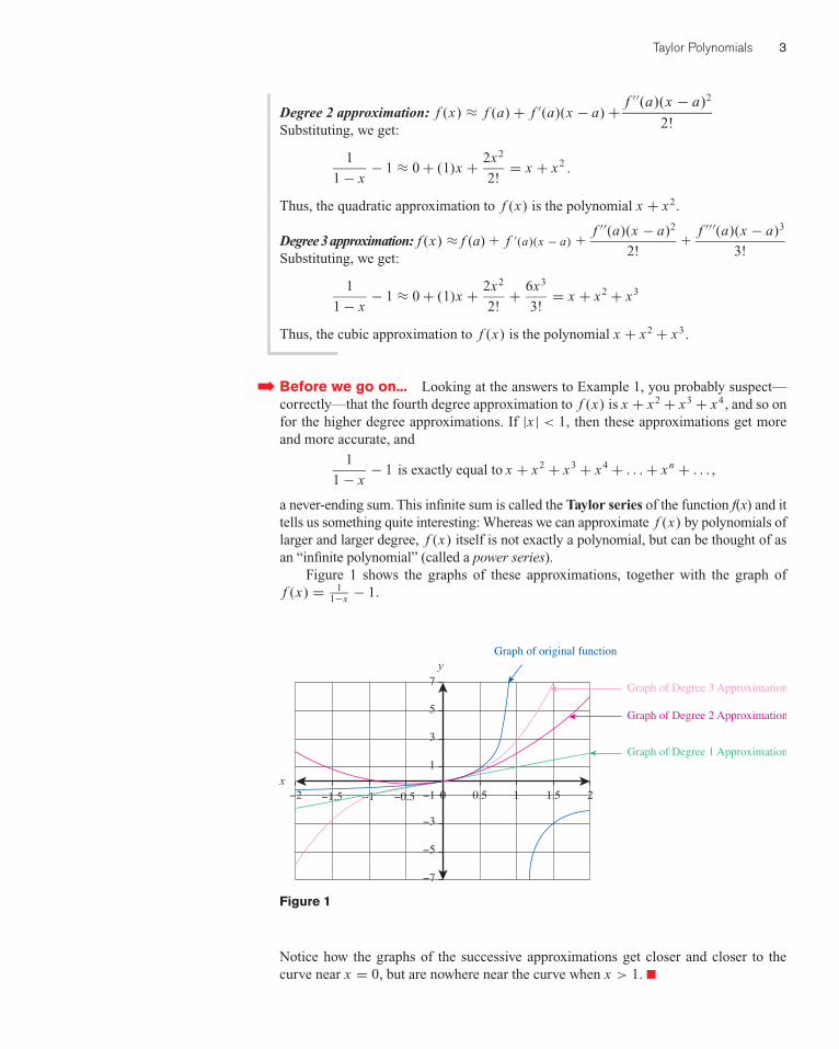
a never-ending sum. This infinite sum is called the Taylor series of the function f(x) and ittells us something quite interesting: Whereas we can approximate f (x) by polynomials oflarger and larger degree, f (x) itself is not exactly a polynomial, but can be thought of asan “infinite polynomial” (called a power series).
Figure 1 shows the graphs of these approximations, together with the graph off (x) = 1
1−x − 1.
Taylor Polynomials 3
−7
−5
−2 −1.5 −1 −0.5 0 0.5 1 1.5 2
−3
−1
1
3
5
7
Graph of original function
Graph of Degree 3 Approximation
Graph of Degree 2 Approximation
Graph of Degree 1 Approximation
x
y
Figure 1
➡
Notice how the graphs of the successive approximations get closer and closer to thecurve near x = 0, but are nowhere near the curve when x > 1. �
EXAMPLE 2 Taylor Polynomial for ex
Find a fifth degree polynomial approximation for ex by expanding the function about zero.
Solution
Once again, we have a = 0, and we need to list all the derivatives up to the fifth, evalu-ating at 0 as we go.
f (x) = ex so f (0) = 1
f ′(x) = ex so f ′(0) = 1
f ′′(x) = ex so f ′′(0) = 1
f ′′′(x) = ex so f ′′′(0) = 1
f (4)(x) = ex so f (4)(0) = 1
f (5)(x) = ex so f (5)(0) = 1
Since the formula for the fifth degree approximation to f (x) is
f (x) ≈ f (0) + f ′(0)x + f ′′(0)x2
2!+ f ′′′(0)x3
3!+ f (4)(0)x4
4!+ f (5)(0)x5
5!,
we get
ex ≈ 1 + x + x2
2!+ x3
3!+ x4
4!+ x5
5!.
as our desired degree 5 approximation.
Before we go on... The approximation in Example 2 turns out to be quite accurate forsmall values of x—even as large as 1. For instance, if we take x = 1, the left-hand side is2.7182 . . ., while the right-hand side is 2.71666 . . ., accurate to within about 0.002. It turnsout (and we shall see why shortly) that the error terms approach zero no matter what thevalue of x , so that
ex = 1 + x + x2
2!+ x3
3!+ x4
4!+ · · · + xn
n!+ · · · .
In particular,
e = e1 = 1 + 1 + 1
2!+ 1
3!+ 1
4!+ · · · + 1
n!+ · · · .
This is in fact the way in which many calculators compute ex and e.If you have a graphing calculator or graphing software, you are urged to graph
several approximations, and compare their graphs with that of ex . �
EXAMPLE 3 Taylor Polynomial for In x
Find the fifth Taylor polynomial for f (x) = ln x around 1.
Solution This time, a = 1.2 We need five derivatives of f :
f (x) = ln x so f (1) = 0
4 Taylor Polynomials
➡
2 We can’t take a = 0. (Why?)
f ′(x) = 1
xso f ′(1) = 1
f ′′(x) = –1
x2so f ′′(1) = –1
f ′′′(x) = 2
x3so f ′′′(1) = 2
f (4)(x) = –6
x4so f (4)(1) = –6
f (5)(x) = 24
x5so f (5)(x) = 24
The fifth Taylor polynomial must be
ln x ≈ 0 + (1)(x − 1) − (1)(x − 1)2
2+ 2(x − 1)3
3!–
6(x − 1)4
4!+ 24(x − 1)5
5!
= (x − 1) − (x − 1)2
2+ (x − 1)3
3− (x − 1)4
4+ (x − 1)5
5
Taylor Polynomials 5
➡
3 And the bridges you design may collapse as a result!
Before we go on... If x < 1, then the remainders go to zero as n gets large, so thatwe can also represent ln x as an infinite polynomial:
ln x = (x − 1) − (x − 1)2
2+ (x − 1)3
3− (x − 1)4
4+ (x − 1)5
5+ · · · �
We’ve been making lots of claims about remainders becoming smaller and smalleras n gets larger, so it is now time to take a careful look at these remainders. Recall thatthe remainder is given by the formula
Rn =∫ x
a
f (n+1)(t)(x − t)n
n!dt.
This formula gives the exact error when f (x) is approximated by the nth Taylor sum. Becauseit is often too cumbersome to evaluate as it stands, we will replace this formula with some-thing more manageable. Our philosophy is the following: Rather than try to get the exact error,we shall judiciously overestimate the magnitude of the error by using a far simpler formula.
What’s the point of overestimating the error?
Look at it this way. The value of e is 2.718281828... If you say that e = 2.718 to within±0.0003, you are estimating the error to be at most ±0.0003 when e is replaced by2.718. In other words, 0.0003 is an overestimation of the actual error; the actual erroris 0.000281828... . By overestimating the error, you are making a correct claim about the value of e. If, instead, you were to underestimate the error, and claim, for instance, that e = 2.718 to within ±0.0002, you would be dead wrong!3
So how do we overestimate the magnitude of Rn?
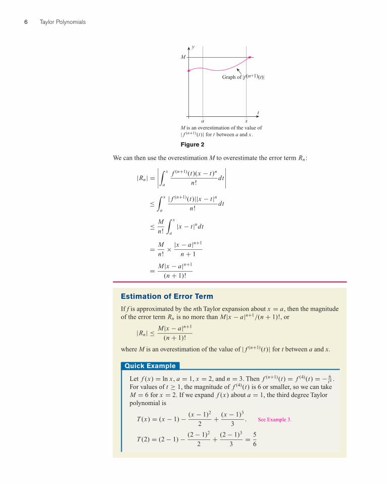
First, we look at the magnitude of the (n + 1)st derivative of f (t ) as t varies betweena and x, and overestimate that by a single number M. (See Figure 2.)
We can then use the overestimation M to overestimate the error term Rn :
|Rn| =∣∣∣∣∣∫ x
a
f (n+1)(t)(x − t)n
n!dt
∣∣∣∣∣≤
∫ x
a
| f (n+1)(t)||x − t |nn!
dt
≤ M
n!
∫ x
a|x − t |ndt
= M
n!× |x − a|n+1
n + 1
= M|x − a|n+1
(n + 1)!
6 Taylor Polynomials
M
Graph of |f (n+1)(t)|
xat
y
M is an overestimation of the value of| f (n+1)(t)| for t between a and x .
Figure 2
Estimation of Error Term
If f is approximated by the nth Taylor expansion about x = a, then the magnitudeof the error term Rn is no more than M|x − a|n+1/(n + 1)!, or
|Rn| ≤ M|x − a|n+1
(n + 1)!
where M is an overestimation of the value of | f (n+1)(t)| for t between a and x.
Quick Example
Let f (x) = ln x , a = 1, x = 2, and n = 3. Then f (n+1)(t) = f (4)(t) = − 6t4 .
For values of t ≥ 1, the magnitude of f (4)(t) is 6 or smaller, so we can takeM = 6 for x = 2. If we expand f (x) about a = 1, the third degree Taylorpolynomial is
T (x) = (x − 1) − (x − 1)2
2+ (x − 1)3
3. See Example 3.
T (2) = (2 − 1) − (2 − 1)2
2+ (2 − 1)3
3= 5
6
Taylor Polynomials 7
0
1000
800
600
400
200
0
0.1 0.2 0.3 0.4 0.5
y
t
Graph of f (t) = 24(1−t)5
EXAMPLE 4 Estimating the Error
Expand f (x) = 1(1−x) − 1 around x = 0 to get a cubic approximation, and estimate the
error if we approximate f (x) by this cubic for x between 0 and 12 .
Solution We already saw in Example 1 that the cubic approximation to f (x) is
T (x) = x + x2 + x3.
To estimate the error, we need to find M. Because n = 3, we need to look at the 4thderivative of f (t), which is 24
(1−t)5 . Now t varies between 0 and x, which is anywherebetween 0 and 1
2 . In other words, t varies between 0 and 12 .
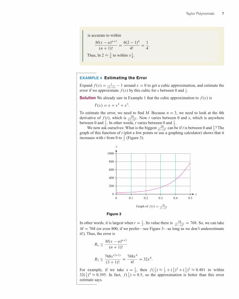
We now ask ourselves: What is the biggest 24(1−t)5 can be if t is between 0 and 1
2 ? Thegraph of this function of t (plot a few points or use a graphing calculator) shows that itincreases with t from 0 to 1
2 (Figure 3).
In other words, it is largest when t = 12 . Its value there is 24
(1− 12 )5 = 768. So, we can take
M = 768 (or even 800, if we prefer—see Figure 3—as long as we don’t underestimateit!). Thus, the error is
Rn ≤ M(x − a)n+1
(n + 1)!
R3 ≤ 768x (3+1)
(3 + 1)!= 768x4
4!= 32x4.
For example, if we take x = 13 , then f ( 1
3 ) ≈ 13 + ( 1
3 )2 + ( 13 )3 ≈ 0.481 to within
32( 13 )4 ≈ 0.395. In fact, f ( 1
3 ) = 0.5, so the approximation is better than this errorestimate says.
is accurate to within
M(x − a)n+1
(n + 1)!= 6(2 − 1)4
4!= 1
4.
Thus, ln 2 ≈ 56 to within ± 1
4 .
Figure 3
EXAMPLE 5 Approximating e
Estimate the error when e is approximated by 1 + 1 + 12! + 1
3! + 14! .
Solution The given polynomial is the fourth Taylor approximation of ex with a = 0and x = 1 (see Example 2). To find M, we look at the fifth derivative of et , which isagain et , and overestimate that for t between 0 and 1. Since the largest value it can have in this range is e1 = e, we can take M = e, or simpler yet, M = 3, since 3 is a con-venient overestimation of e. Thus, the error is
R4 ≤ 3(1 − 0)4+1
(4 + 1)!= 3
120= 0.025.
So, we can be sure that e ≈ 1 + 1 + 12! + 1
3! + 14! ≈ 2.708 to within 0.025.
EXAMPLE 6 Approximating the Natural Logarithm
Find the fifth Taylor polynomial for f (x) = ln x around a = 1, and estimate the errorterm if we use this polynomial to approximate ln 1.1.
Solution We already calculated this polynomial in Example 3, where we obtained
ln x ≈ (x − 1) − (x − 1)2
2+ (x − 1)3
3− (x − 1)4
4+ (x − 1)5
5.
For the error term, we want to approximate ln 1.1, so x = 1.1. We look at the magnitudeof the sixth derivative, | f (6)(t)| = 120/t6, and estimate its largest value as t ranges from1 to 1.1. It is largest when t = 1, so we can take M = 120. Thus, the error is
R5 ≤ 120(1.1 − 1)5+1
(5 + 1)!= 0.00012
720≈ 0.000000167 .
Before we go on... The point of Example 6 is that there is a way to calculate naturallogarithms using ordinary arithmetic. For example, we can estimate ln 1.1 as
ln 1.1 ≈ (1.1 − 1) − (1.1 − 1)2
2+ (1.1 − 1)3
3− (1.1 − 1)4
4
�(1.1 − 1)5
5≈ 0.0953103.
How accurate is this? The error is no larger than 0.000000167, so we can say withabsolute certainty that ln 1.1 is somewhere between 0.0953101 and 0.0953105. �
Sometimes, we would like to approximate a certain quantity to a specified numberof decimal places.
8 Taylor Polynomials
➡
What exactly does it mean to approximate a quantity to, say, three decimal places?
If we already know the exact value of the quantity, then we simply round it to three decimal places. Notice that doing so may change the quantity by as much as0.0005 = 5 × 10⁻⁴. (For example, rounding 0.1005 to three decimal places produces0.101, and so we have changed it by 0.0005.) This motivates the following definition:
Taylor Polynomials 9
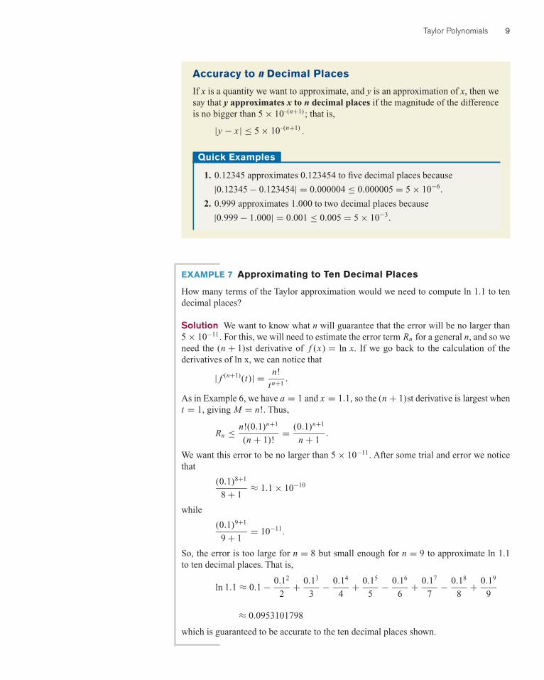
Accuracy to n Decimal Places
If x is a quantity we want to approximate, and y is an approximation of x, then wesay that y approximates x to n decimal places if the magnitude of the differenceis no bigger than 5 × 10–(n+1) ; that is,
|y − x | ≤ 5 × 10–(n+1) .
Quick Examples
1. 0.12345 approximates 0.123454 to five decimal places because
2. 0.999 approximates 1.000 to two decimal places because
|0.999 − 1.000| = 0.001 ≤ 0.005 = 5 × 10⁻³.
EXAMPLE 7 Approximating to Ten Decimal Places
How many terms of the Taylor approximation would we need to compute ln 1.1 to tendecimal places?
Solution We want to know what n will guarantee that the error will be no larger than5 × 10−11. For this, we will need to estimate the error term Rn for a general n, and so weneed the (n + 1)st derivative of f (x) = ln x. If we go back to the calculation of thederivatives of ln x, we can notice that
| f (n+1)(t)| = n!
tn+1.
As in Example 6, we have a = 1 and x = 1.1, so the (n + 1)st derivative is largest whent = 1, giving M = n!. Thus,
Rn ≤ n!(0.1)n+1
(n + 1)!= (0.1)n+1
n + 1.
We want this error to be no larger than 5 × 10⁻¹¹. After some trial and error we noticethat
(0.1)8+1
8 + 1≈ 1.1 × 10⁻¹⁰
while
(0.1)9+1
9 + 1= 10−11.
So, the error is too large for n = 8 but small enough for n = 9 to approximate ln 1.1 to ten decimal places. That is,
ln 1.1 ≈ 0.1 − 0.12
2+ 0.13
3− 0.14
4+ 0.15
5− 0.16
6+ 0.17
7− 0.18
8+ 0.19
9
≈ 0.0953101798
which is guaranteed to be accurate to the ten decimal places shown.
10 Taylor Polynomials
−→
−→
−→
−→
−→−→
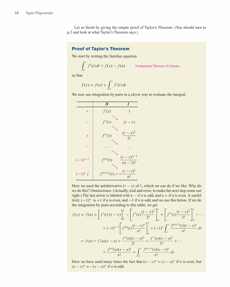
Let us finish by giving the simple proof of Taylor’s Theorem. (You should turn to p.2 and look at what Taylor’s Theorem says.)
Proof of Taylor’s Theorem
We start by writing the familiar equation∫ x
af ′(t) dt � f (x) − f (a) Fundamental Theorem of Calculus
so that
f (x) = f (a) +∫ x
af ′(t) dt.
We now use integration by parts in a clever way to evaluate the integral.
D I
+ f ′(t) 1
− f ′′(t) (t − x)
+ f ′′′(t)(t − x)2
2!
− . . . . . .
(−1)n−1 f (n)(t)(t − x)n−1
(n − 1)!
(−1)n∫
f (n+1)(t)(t − x)n
n!
Here we used the antiderivative (t − x) of 1, which we can do if we like. Why dowe do this? Omniscience. (Actually, trial and error, to make the next step come outright.) The last arrow is labeled with a − if n is odd, and a + if n is even. A usefultrick: (−1)n is +1 if n is even, and −1 if n is odd, and we use this below. If we dothe integration by parts according to this table, we get
f (x) = f (a) +[
f ′(t) (t − x)
]x
a
−[
f ′′(t)(t − x)2
2!
]x
a
+[
f ′′′(t)(t − x)3
3!
]x
a
− · · ·
� (−1)n−1
[f (n)(t)
(t − x)n
n!
]x
a
+ (−1)n
∫ x
a
f (n+1)(t)(t − x)n
n!dt
= f (a) + f ′(a)(x − a) + f ′′(a)(x − a)2
2!+ f ′′′(a)(x − a)3
3!+ · · ·
� f (n)(a)(x − a)n
n!+
∫ x
a
f (n+1)(t)(x − t)n
n!dt
Here we have used many times the fact that (a − x)n = (x − a)n if n is even, but(a − x)n = −(x − a)n if n is odd.
� more advanced
In Exercises 1–14, find the 5th Taylor polynomials of the func-tions around the given points.
1. f (x) = x3 + 2x2 − 3x + 1; a = 0
2. f (x) = x3 − x2 + 4x + 10; a = 0
3. f (x) = x3 + 2x2 − 3x + 1; a = 1
4. f (x) = x3 − x2 + 4x + 10; a = 1
5. f (x) = ln(1 − x); a = 0
6. f (x) = ln(2 − x); a = 0
7. f (x) = ex ; a = 0
8. f (x) = e−x ; a = 0
9. f (x) = e−x2 ; a = 0
10. f (x) = e(x−1)2 ; a = 1
11. 1x−1 ; x = 0
12. 1(1−x)2 ; x = 0
13.√
x; x = 1
14. x1/3; x = 1
In Exercises 15–20, find the Taylor polynomial around x = aapproximating f(x) to within ±0.0001. Calculate the approximationgiven by the Taylor polynomial, and compare to the answer givenby a calculator.
15. � f (x) = ex ; a = 0, approximate f (1)
16. � f (x) = ex ; a = 0, approximate f (1/2)
17. � f (x) = 1x ; a = 1, approximate f (1.1)
Taylor Polynomials 11
EXERCISES18. � f (x) = 1
x ; a = 1, approximate f (0.9)
19. � f (x) = √x; a = 100, approximate f(101)
20. � f (x) = √x; a = 100, approximate f(99)
21. � How many terms of the Taylor series around x = 0 couldyou use to approximate e to 3 decimal places?
22. � How many terms of the Taylor series around x = 0 couldyou use to approximate e to 4 decimal places?
23. � To how many decimal places is the approximation1
1 − x− 1 ≈ x + x2 + x3
in Example 4 accurate when x = 0.1?
24. � To how many decimal places is the approximation
ln 1.1 ≈ 0.1 − 0.12
2+ 0.13
3− 0.14
4+ 0.15
5
in Example 7 accurate?
APPLICATIONS
25. � Investing The Amex Gold BUGS4 Index was at 150points in January 2003, decreasing at a rate of 14.5points/month, and accelerating at 3.6 points/month2.
(a) Taking t as time in months since January 2003, obtainthe first and second Taylor polynomials of the BUGSindex b as a function of t around t = 0.
(b) Use the second order Taylor polynomial to approxi-mate the value of the index in January 2004, andcompare the predicted value with the (approximate)actual value.
263
233
203
173
143
113
Jan
’03
Feb
’03
Apr
’03
Jun
’03
Aug
’03
Oct
’03
Dec
’03
Jan
’04
Mar
’04
Index
Source: www.amex.com
4BUGS stands for “basket of unhedged gold stocks.”
Art for Exercise 25
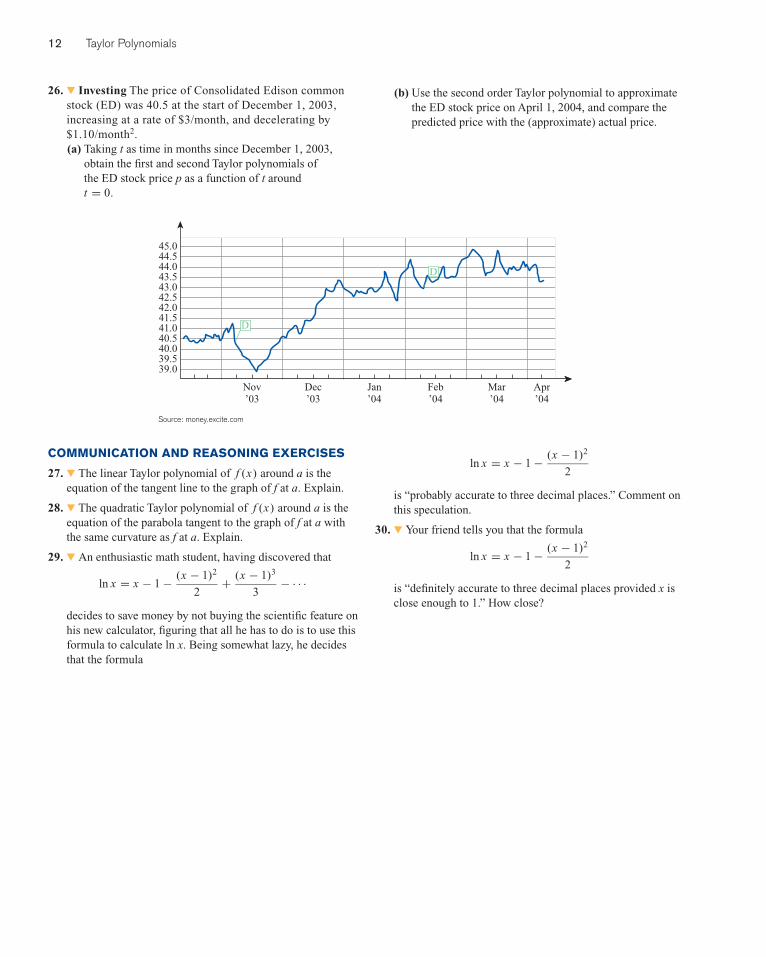
26. � Investing The price of Consolidated Edison commonstock (ED) was 40.5 at the start of December 1, 2003,increasing at a rate of $3/month, and decelerating by$1.10/month2.(a) Taking t as time in months since December 1, 2003,
obtain the first and second Taylor polynomials of the ED stock price p as a function of t around t = 0.
12 Taylor Polynomials
(b) Use the second order Taylor polynomial to approximatethe ED stock price on April 1, 2004, and compare thepredicted price with the (approximate) actual price.
27. � The linear Taylor polynomial of f (x) around a is theequation of the tangent line to the graph of f at a. Explain.
28. � The quadratic Taylor polynomial of f (x) around a is theequation of the parabola tangent to the graph of f at a withthe same curvature as f at a. Explain.
29. � An enthusiastic math student, having discovered that
ln x = x − 1 − (x − 1)2
2+ (x − 1)3
3− · · ·
decides to save money by not buying the scientific feature onhis new calculator, figuring that all he has to do is to use thisformula to calculate ln x. Being somewhat lazy, he decidesthat the formula
ln x = x − 1 − (x − 1)2
2
is “probably accurate to three decimal places.” Comment onthis speculation.
30. � Your friend tells you that the formula
ln x = x − 1 − (x − 1)2
2
is “definitely accurate to three decimal places provided x isclose enough to 1.” How close?
Source: money.excite.com
TA
YLO
R P
OLY
NO
MIA
LS
: A
NS
WE
RS
TO
OD
D-N
UM
BE
RE
D E
XE
RC
ISE
S
Taylor Polynomials: Answers to Odd-Numbered Exercises
21. 8 terms altogether (n = 7)23. R3 ≤ 32x4 = 32(0.1)4 = 0.0032. Since this is less than0.005, the approximation is accurate to 2 decimal places.25. a. First Taylor Polynomial: b(t) ≈ 150 − 14.5t ; Second Taylor Polynomial: b(t) ≈ 150 − 14.5t + 1.8t2
b. b(12) ≈ 235.2 points. The actual value was around 220 points.27. The linear Taylor polynomial is f (a) + f ′(a)(x − a), whichis the equation of the line through (a, f (a)) with slope f ′(a).29. The speculation is unfounded. Take x = 1.5. Then ln 1.5 ≈ 0.4055, whereas the second Taylor polynomial isT (1.5) = 1.5 − 1 − (1.5 − 1)2/2 = 0.375, so the error is much larger than 0.005.