67
Tahir Muhammad Fall 2010 D IGITAL S IGNAL P ROCESSING Lab Manual UNIVERSITY OF ENGINEERING AND TECHNOLOGY, TAXILA

Tahir Muhammad
Fall 2010
DIGITAL SIGNAL PROCESSING Lab Manual
UNIVERSITY OF ENGINEERING AND TECHNOLOGY, TAXILA

Digital Signal Processing Lab Manual Fall 2010
1
TABLE OF CONTENTS
LAB PAGE 1. GETTING STARTED WITH MATLAB 2
2. SIGNALS IN MATLAB 16 3. DISCRETE TIME SYSTEMS 21 4. FREQUENCY ANALYSIS 28 5. Z-TRANSFORM 33
6. SAMPLING, A/D CONVERSION AND D/A
CONVERSION 39
7. FIR AND IIR FILTER DESIGN IN MATLAB 42
8. INTRODUCTION TO TEXAS INSTRUMENTS
TMS320C6713 DSP STARTER KIT (DSK) DIGITAL
SIGNALPROCESSING BOARD 45
9. INTERRUPTS AND VISUALIZATION TOOLS 56
10. SAMPLING IN CCS AND C6713 63
11. FIR FILTER DESIGN IN CCS 64
12. IIR FILTER DESING IN CCS 65
13. PROJECT

Digital Signal Processing Lab Manual Fall 2010
2
LAB 1: GETTING STARTED WITH
MATLAB
Introduction This lab is to familiarize the students with MATLAB environment
through it some preliminary MATLAB functions will be also covered.
Procedure: Students are required to go through the steps explained below and then complete the
exercises given at the end of the lab.
1. Introduction to MATLAB
i. Too add comment the following symbol is used "%".
ii. Help is provided by typing “help” or if you know the topic then “help
function_name” or “doc function_name”.
iii. If you don't know the exact name of the topic or command you are looking
for,type "lookfor keyword" (e.g., "lookfor regression")
iv. Three dots “...” are used to continue a statement to next line (row).
v. If after a statement “;” is entered then MATLAB will not display the result of
the statement entered otherwise result would be displayed.
vi. Use the up-arrow to recall commands without retyping them (and down
arrow to go forward in commands).
vii. MATLAB is case sensitive so “taxila” is not same as “TAXILA”
2. Basic functionalities of MATLAB Defining a scalar:
x=1
x =
1
Defining a column vector v = [1;2;3]
v =
1
Digital Signal Processing Lab Manual Fall 2010
3
2
3
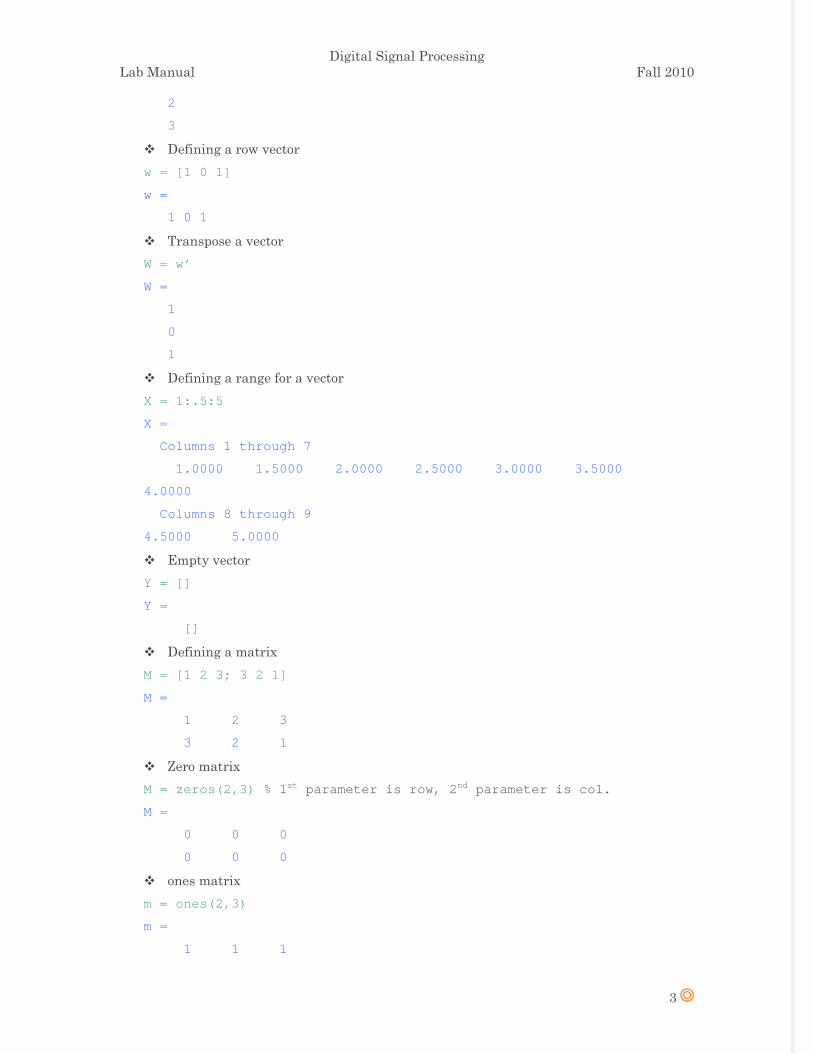
Defining a row vector w = [1 0 1]
w =
1 0 1
Transpose a vector W = w’
W =
1
0
1
Defining a range for a vector X = 1:.5:5
X =
Columns 1 through 7
1.0000 1.5000 2.0000 2.5000 3.0000 3.5000
4.0000
Columns 8 through 9
4.5000 5.0000
Empty vector Y = []
Y =
[]
Defining a matrix M = [1 2 3; 3 2 1]
M =
1 2 3
3 2 1
Zero matrix M = zeros(2,3) % 1st parameter is row, 2nd parameter is col.
M =
0 0 0
0 0 0 ones matrix
m = ones(2,3)
m =
1 1 1

Digital Signal Processing Lab Manual Fall 2010
4
1 1 1
The identity matrix I = eye(3)
I =
1 0 0
0 1 0
0 0 1
Define a random matrix or vector R = rand(1,3)
R =
0.9501 0.2311 0.6068
Access a vector or matrix R(3)
ans =
0.6068
or R(1,2)
ans =
0.2311
Access a row or column of matrix I(2,:) %2nd row
ans =
0 1 0
I(:,2) %2nd col
ans =
0
1
0
I(1:2,1:2)
ans =
1 0
0 1
size and length size(I)
ans =

Digital Signal Processing Lab Manual Fall 2010
5
3 3
length(I)
ans =
3
already defined variable by a user who
Your variables are:
I M R W X Y ans m t v y
3. Operations on vector and matrices in MATLAB MATLAB utilizes the following arithmetic operatops;
+ Addition
- Subtraction
* Multiplication
/ Division
^ Power Operator
‘ transpose
Some built in functions in MATLAB
abs magnitude of a number (absolute value for real numbers)
angle angle of a complex number, in radians
cos cosine function, assumes argument is in radians
sin sine function, assumes argument is in radians
exp exponential function
Arithmetic operations x=[ 1 2 3 4 5]
x =
1 2 3 4 5
x= 2 * x
x =
2 4 6 8 10
x= x / 2
x =
1 2 3 4 5
y = [ 1 2 3 4 5 ]
Digital Signal Processing Lab Manual Fall 2010
6
y =
1 2 3 4 5
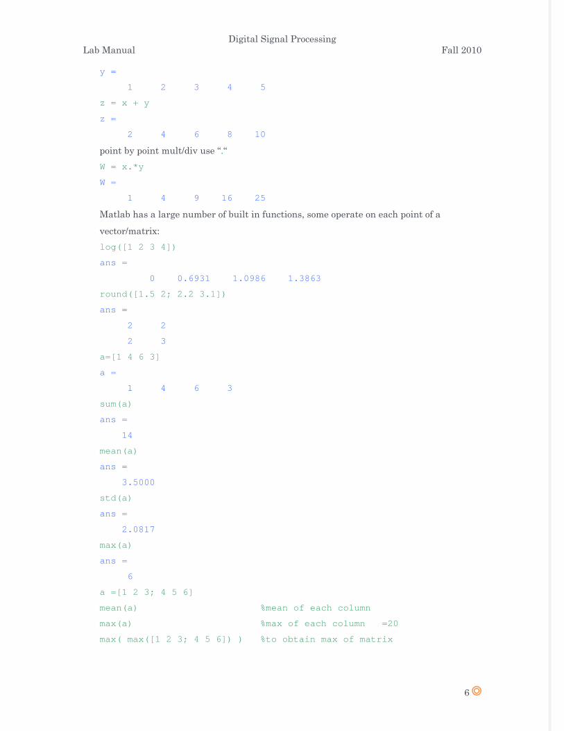
z = x + y
z =
2 4 6 8 10
point by point mult/div use “.“ W = x.*y
W =
1 4 9 16 25
Matlab has a large number of built in functions, some operate on each point of a
vector/matrix: log([1 2 3 4])
ans =
0 0.6931 1.0986 1.3863
round([1.5 2; 2.2 3.1])
ans =
2 2
2 3
a=[1 4 6 3]
a =
1 4 6 3
sum(a)
ans =
14
mean(a)
ans =
3.5000
std(a)
ans =
2.0817
max(a)
ans =
6
a =[1 2 3; 4 5 6]
mean(a) %mean of each column
max(a) %max of each column =20
max( max([1 2 3; 4 5 6]) ) %to obtain max of matrix

Digital Signal Processing Lab Manual Fall 2010
7
4. Relational operators in MATLAB Relational operators: =(equal), ~=3D (not equal), etc.
Let a = [1 1 3 4 1]
a =
1 1 3 4 1
ind = (a == 1)
ind =
1 1 0 0 1
ind = (a < 1)
ind =
0 0 0 0 0
ind = (a > 1)
ind =
0 0 1 1 0
ind = (a <= 1)
ind =
1 1 0 0 1
ind = (a >= 1)
ind =
1 1 1 1 1
ind = (a ~= 1)
ind =
0 0 1 1 0
5. Control Flow in MATLAB
To control the flow of commands, the makers of MATLAB supplied four devices a
programmer can use while writing his/her computer code
• the for loops

Digital Signal Processing Lab Manual Fall 2010
8
• the while loops
• the if-else-end constructions
• the switch-case constructions
Syntax of the for loop is shown below
for k = array
commands
end
The commands between the for and end statements are executed for all %values stored
in the array.
Suppose that one-need values of the sine function at eleven evenly %spaced points n/10,
for n = 0, 1, …, 10. To generate the numbers in %question one can use the for loop for n=0:10
x(n+1) = sin(pi*n/10);
end
x =
Columns 1 through 7
0 0.3090 0.5878 0.8090 0.9511 1.0000
0.9511
Columns 8 through 11
0.8090 0.5878 0.3090 0.0000
The for loops can be nested H = zeros(5);
for k=1:5
for l=1:5
H(k,l) = 1/(k+l-1);
end
end
H =
1.0000 0.5000 0.3333 0.2500 0.2000
0.5000 0.3333 0.2500 0.2000 0.1667
0.3333 0.2500 0.2000 0.1667 0.1429
0.2500 0.2000 0.1667 0.1429 0.1250
0.2000 0.1667 0.1429 0.1250 0.1111
Syntax of the while loop is
while expression
statements

Digital Signal Processing Lab Manual Fall 2010
9
end
This loop is used when the programmer does not know the number of repetitions a priori.
Here is an almost trivial problem that requires a use of this loop. Suppose that the
number is divided by 2. The resulting quotient is divided by 2 again. This process is
continued till the current quotient is less than or equal to 0.01. What is the largest
quotient that is greater than 0.01?
To answer this question we write a few lines of code q = pi;
while q > 0.01
q = q/2;
end
q =
0.0061
Syntax of the simplest form of the construction under discussion is
if expression
commands
end
This construction is used if there is one alternative only. Two alternatives require the
construction
if expression
commands (evaluated if expression is true)
else
commands (evaluated if expression is false)
end
If there are several alternatives one should use the following construction
if expression1
commands (evaluated if expression 1 is true)
elseif expression 2
commands (evaluated if expression 2 is true)
elseif …
...
else
commands (executed if all previous expressions evaluate to false)
end
Syntax of the switch-case construction is
switch expression (scalar or string)

Digital Signal Processing Lab Manual Fall 2010
10
case value1 (executes if expression evaluates to value1)
commands
case value2 (executes if expression evaluates to value2)
commands
...
otherwise
statements
end
Switch compares the input expression to each case value. Once the %match is found it
executes the associated commands.
In the following example a random integer number x from the set {1, 2, … , 10} is
generated. If x = 1 or x = 2, then the message Probability = 20% is displayed to the
screen. If x = 3 or 4 or 5, then the message Probability = 30 is displayed, otherwise the
message Probability = 50% is generated. The script file fswitch utilizes a switch as a tool
%for handling all cases mentioned above % Script file fswitch.
x = ceil(10*rand); % Generate a random integer in {1, 2, ... , 10}
switch x
case {1,2}
disp('Probability = 20%');
case {3,4,5}
disp('Probability = 30%');
otherwise
disp('Probability = 50%');
end
Note: use of the curly braces after the word case. This creates the so called cell
array rather than the one-dimensional array, which %requires use of the
square brackets.
6. Creating functions using m-files Files that contain a computer code are called the m-files. There are two kinds of m-files:
the script files and the function files. Script files do not take the input arguments or
return the output arguments. The function files may take input arguments or return
output arguments. To make the m-file click on File next select New and click on M-File
from the pull-down menu. You will be presented with the MATLAB Editor/Debugger
screen. Here you will type your code, can make %changes, etc. Once you are done with

Digital Signal Processing Lab Manual Fall 2010
11
typing, click on File, in the MATLAB Editor/Debugger screen and select Save As… .
Chose a name for your file, e.g., firstgraph.m and click on Save. Make sure that your
file is saved in the directory that is in MATLAB's search path. If you %have at least two
files with duplicated names, then the one that occurs first in MATLAB's search path will
be executed.
To open the m-file from within the Command Window type edit firstgraph %and then
press Enter or Return key.
Here is an example of a small script file % Script file firstgraph.
x = -10*pi:pi/100:10*pi;
y = sin(x)./x;
plot(x,y)
grid
Enter this code in the MATLAB editor and save it as firstgraph.m. This function call be
called from command line as firstgraph
Here is an example of a function file function [b, j] = descsort(a)
% Function descsort sorts, in the descending order, a real array a.
% Second output parameter j holds a permutation used to obtain
% array b from the array a.
[b ,j] = sort(-a);
b = -b;
Enter this code in the MATLAB editor and save it as descsort.m . This function call be
called from command line as X=1:10
descsort(X)
7. Graphs in MATLAB save the script file and the run it
Script file graph1.
Graph of the rational function y = x/(1+x^2). for n=1:2:5
n10 = 10*n;
x = linspace(-2,2,n10);
y = x./(1+x.^2);

Digital Signal Processing Lab Manual Fall 2010
12
plot(x,y,'r')
title(sprintf('Graph %g. Plot based upon n = %g points.' ...
,(n+1)/2, n10))
axis([-2,2,-.8,.8])
xlabel('x')
ylabel('y')
grid
pause(3)
end%Several graphs using subplot
graph1
Script file graph2.
Several plots of the rational function y = x/(1+x^2)
in the same window. k = 0;
for n=1:3:10
n10 = 10*n;
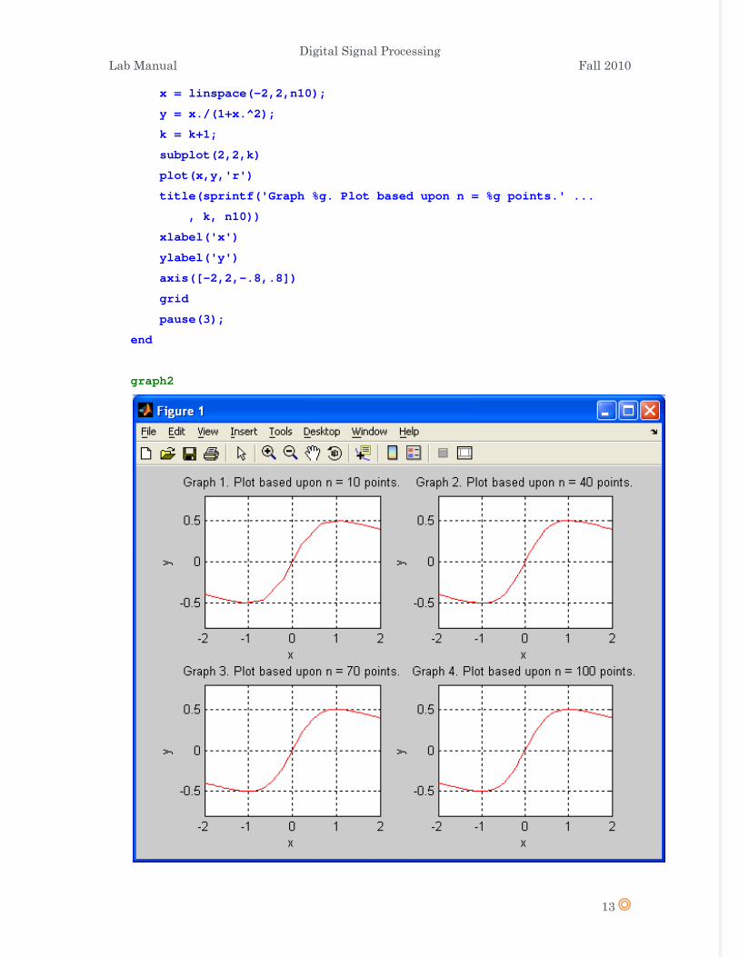
Digital Signal Processing Lab Manual Fall 2010
13
x = linspace(-2,2,n10);
y = x./(1+x.^2);
k = k+1;
subplot(2,2,k)
plot(x,y,'r')
title(sprintf('Graph %g. Plot based upon n = %g points.' ...
, k, n10))
xlabel('x')
ylabel('y')
axis([-2,2,-.8,.8])
grid
pause(3);
end
graph2
Digital Signal Processing Lab Manual Fall 2010
14
Exercises:
1. Operate with the vectors
V1 = [1 2 3 4 5 6 7 8 9 0]
V2 = [0.3 1.2 0.5 2.1 0.1 0.4 3.6 4.2 1.7 0.9]
V3 = [4 4 4 4 3 3 2 2 2 1]
a) Calculate, respectively, the sum of all the elements in vectors V1, V2, and V3
b) How to get the value of the fifth element of each vector?
What happens if we execute the command V1(0) and V1(11)?
Remember if a vector has N elements, their subscripts are from 1 to N.
c) Generate a new vector V4 from V2, which is composed of the first five elements of V2.
d) Generate a new vector V5 from V2, which is composed of the last five elements of V2.
e) Derive a new vector V6 from V2, with its 6th element omitted.
f) Derive a new vector V7 from V2, with its 7th element changed to 1.4.
g) Derive a new vector V8 from V2, whose elements are the 1st, 3rd, 5th, 7th, and 9th
elements of V2
h) What are the results of
9-V1
V1*5
V1+V2
V1-V3
V1.*V2
V1*V2
V1.^2
V1.^V3
V1^V3
V1 == V3
V1>6
V1>V3
V3-(V1>2)
(V1>2) & (V1<6)
(V1>2) | (V1<6)
any(V1)
all(V1)
2. Compare a script and a function

Digital Signal Processing Lab Manual Fall 2010
15
a) Write a script: In the main menu of Matlab, select
file -> new -> M-file
A new window will pop up. Input the following commands:
x = 1:5;
y = 6:10;
g = x+y;
and then save the file as myscript.m under the default path matlab/work
b) Write a function: Create a new m file following the procedure of above. Type in the
commands:
function g = myfunction(x,y)
g = x + y;
and then save it as myfunction.m
i. Compare their usage
run the commands one by one:
myscript
x
y
g
z = myscript (error?)
ii. Run command clear all to remove all variables from memory
iii. Run the commands one by one:
x = 1:5;
y = 6:10;
myfunction (error?)
z = myfunction(x,y)
g (error?)
a = 1:10;
b = 2:11;
myfunction(a,b)

Digital Signal Processing Lab Manual Fall 2010
16
LAB 2: SINGALS IN MATLAB
Introduction
Signals are broadly classified into continous and discrete signals. A continuous signal will be
denoted by x(t), in which the variable t can represent any physical quantity. A discrete
signal will be denoted x[n], in which the variavble n is integer value. In this lab we will
learn to represent and operate on signals in MATLAB. The variables t and n are assumed to
represent time.
1. Continous Time Signals For the following: Run the following three lines and explain why the plots are different.
Provide the snapshots of the plots for each step given below.
i. close all, clear all
t = 0:2*pi; plot(t,sin(t))
figure
t = 0:0.2:2*pi; plot(t,sin(t))
figuret = 0:0.02:2*pi; plot(t,sin(t))
For the last graph, add a title and axis labels with: title('CT signal plot')
xlabel('t (Seconds)')
ylabel('y(t)')
Change the axis with: axis([0 2*pi -1.2 1.2])
ii. Put two plots on the same axis t = 0:0.2:2*pi; plot(t,sin(t),t,sin(2*t))
iii. Produce a plot without connecting the points
t = 0:0.2:2*pi; plot(t,sin(t),'.')
Try the following command
Digital Signal Processing Lab Manual Fall 2010
17
t = 0:0.2:2*pi; plot(t,sin(t),t,sin(t),'r.')
Question 1: What does ‘r’ do?
Question 2: What does ‘hold’ do? Type doc hold at MATLAB command line for help.
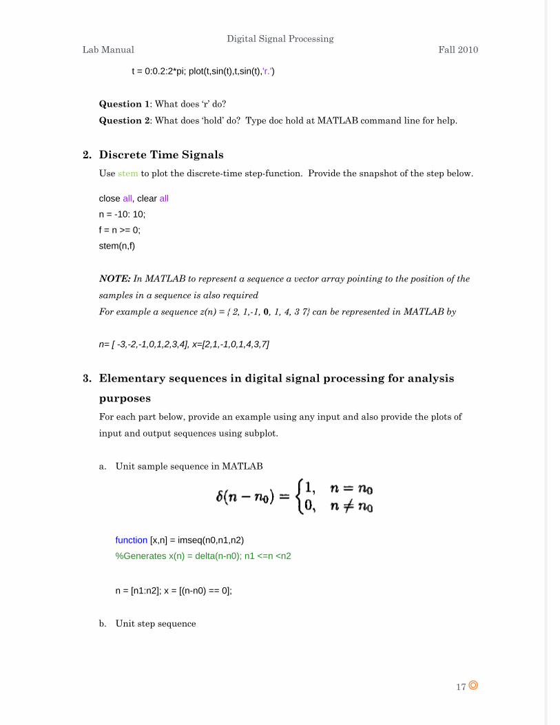
2. Discrete Time Signals Use stem to plot the discrete-time step-function. Provide the snapshot of the step below.
close all, clear all n = -10: 10; f = n >= 0; stem(n,f)
NOTE: In MATLAB to represent a sequence a vector array pointing to the position of the
samples in a sequence is also required
For example a sequence z(n) = { 2, 1,-1, 0, 1, 4, 3 7} can be represented in MATLAB by
n= [ -3,-2,-1,0,1,2,3,4], x=[2,1,-1,0,1,4,3,7]
3. Elementary sequences in digital signal processing for analysis
purposes For each part below, provide an example using any input and also provide the plots of
input and output sequences using subplot.
a. Unit sample sequence in MATLAB
function [x,n] = imseq(n0,n1,n2) %Generates x(n) = delta(n-n0); n1 <=n <n2 n = [n1:n2]; x = [(n-n0) == 0];
b. Unit step sequence

Digital Signal Processing Lab Manual Fall 2010
18
function [x,n] = stepseq(n0,n1,n2) %Generates x(n) = u(n-n0); n <= n <= n2 n = [n1: n2]; x = [(n-n0) >= 0];
c. Real Valued Exponential sequence
n = [0:10]; x = (0.9).^n
d. Complex valued exponential sequence
n = [0:10]; x = exp((2+3j)*n)
e. Sinusoidal sequence
n = [0:10]; x = 3*cos(0.1*pi*n+pi/3) + 2*sin(0.5*pi*n)
4. Operations on Sequence a. Signal addition
It is implemented in MATLAB by the arithmetic operator “+”. However the lengths
of x1(n) and x2(n) must be the same. We can use the following function for addition
function [y,n] = sigadd(x1,n1,x2,n2) % y(n) = x1(n) + x2(n) n = min(min(n1),min(n2)):max(max(n1),max(n2)); y1 = zeros(1,length(n)); y2 = y1; y1(find((n>=min(n1))&(n<=max(n1))==1))=x1;
Digital Signal Processing Lab Manual Fall 2010
19
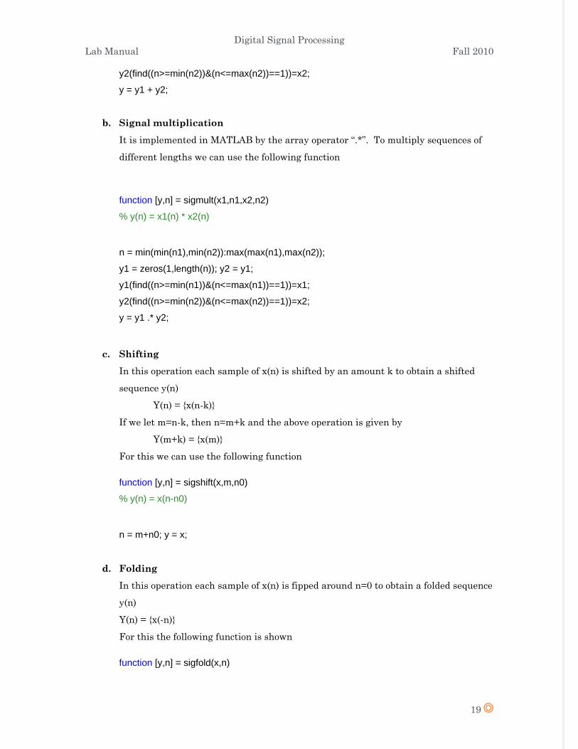
y2(find((n>=min(n2))&(n<=max(n2))==1))=x2; y = y1 + y2;
b. Signal multiplication
It is implemented in MATLAB by the array operator “.*”. To multiply sequences of
different lengths we can use the following function
function [y,n] = sigmult(x1,n1,x2,n2) % y(n) = x1(n) * x2(n) n = min(min(n1),min(n2)):max(max(n1),max(n2)); y1 = zeros(1,length(n)); y2 = y1; y1(find((n>=min(n1))&(n<=max(n1))==1))=x1; y2(find((n>=min(n2))&(n<=max(n2))==1))=x2; y = y1 .* y2;
c. Shifting
In this operation each sample of x(n) is shifted by an amount k to obtain a shifted
sequence y(n)
Y(n) = {x(n-k)}
If we let m=n-k, then n=m+k and the above operation is given by
Y(m+k) = {x(m)}
For this we can use the following function
function [y,n] = sigshift(x,m,n0) % y(n) = x(n-n0) n = m+n0; y = x;
d. Folding
In this operation each sample of x(n) is fipped around n=0 to obtain a folded sequence
y(n)
Y(n) = {x(-n)}
For this the following function is shown
function [y,n] = sigfold(x,n)
Digital Signal Processing Lab Manual Fall 2010
20
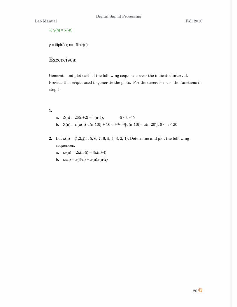
% y(n) = x(-n) y = fliplr(x); n= -fliplr(n);
Excercises:
Generate and plot each of the following sequences over the indicated interval.
Provide the scripts used to generate the plots. For the excercises use the functions in
step 4.
1.
a. Z(n) = 2δ(n+2) – δ(n-4), -5 ≤ δ ≤ 5
b. X(n) = n[u(n)-u(n-10)] + 10 e-0.3(n-10)[u(n-10) – u(n-20)], 0 ≤ n ≤ 20
2. Let x(n) = {1,2,3,4, 5, 6, 7, 6, 5, 4, 3, 2, 1}, Determine and plot the following
sequences.
a. x1(n) = 2x(n-5) – 3x(n+4)
b. x2(n) = x(3-n) + x(n)x(n-2)

Digital Signal Processing Lab Manual Fall 2010
21
LAB 3: DISCRETE TIME SYSTEMS
Introduction
Mathematically, a discrete-time system is described as an operator T[.] that takes a sequence
x(n) called excitation and transforms it into another sequence y(n) (called response). Discrete
time systems can be classified into two categories i) LTI systems ii) NON-LTI systems. A
discrete system T[.] is a linear operator L[.] if and only if L[.] satisfies the principle of
superposition, namely
L[a1x1(n) + a2x2(n)] = a1L[x1(n)] + a2Lx2(n)] and
A discrete system is time-invariant if
Shifting the input only causes the same shift in the output
A system is said to be bounded-input bounded-output(BIBO) stable if every bounded input
produces a bounded output.
An LTI system is BIBO stable if and only if its impulse response is absolutely summable.
A system is said to be causal if the ouput at index n0 depends only on the input up to and
including the index no; that is output does not depend on the future values of the input. An
LTI system is causal if and only if the impulse response is
1. Linearity and Non-Linearity We now investigate the linearity property of a causal system of described by following
equation
Digital Signal Processing Lab Manual Fall 2010
22
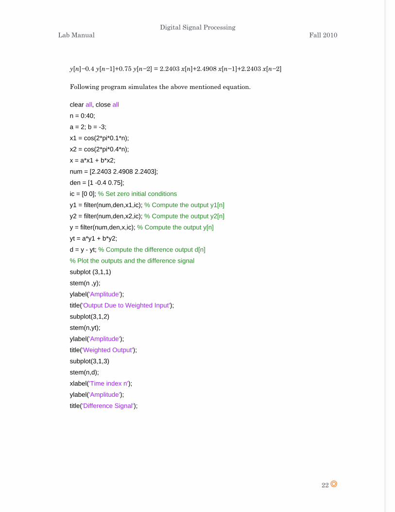
y[n]−0.4 y[n−1]+0.75 y[n−2] = 2.2403 x[n]+2.4908 x[n−1]+2.2403 x[n−2]
Following program simulates the above mentioned equation.
clear all, close all n = 0:40; a = 2; b = -3; x1 = cos(2*pi*0.1*n); x2 = cos(2*pi*0.4*n); x = a*x1 + b*x2; num = [2.2403 2.4908 2.2403]; den = [1 -0.4 0.75]; ic = [0 0]; % Set zero initial conditions y1 = filter(num,den,x1,ic); % Compute the output y1[n] y2 = filter(num,den,x2,ic); % Compute the output y2[n] y = filter(num,den,x,ic); % Compute the output y[n] yt = a*y1 + b*y2; d = y - yt; % Compute the difference output d[n] % Plot the outputs and the difference signal subplot (3,1,1) stem(n ,y); ylabel('Amplitude'); title('Output Due to Weighted Input'); subplot(3,1,2) stem(n,yt); ylabel('Amplitude'); title('Weighted Output'); subplot(3,1,3) stem(n,d); xlabel('Time index n'); ylabel('Amplitude'); title('Difference Signal');

Digital Signal Processing Lab Manual Fall 2010
23
Question 1: Run above program and compare y[n] obtained with weighted input with
yt[n] obtained by combining the two outputs y1[n] and y2[n] with the same weights. Are
these two sequences equal? Is this system linear?
Exercise 1: Consider another system described by y[n] = x[n] x[n − 1]. Modify given
program to compute the output sequences y1[n], y2[n], and y[n] of the above system.
Compare y[n] with yt[n]. Are these two sequences equal? Is this system linear?
2. Time-Invariant and Time-Varying Systems We next investigate the time-invariance property. Following Program simulates
following difference equation
y[n]−0.4 y[n−1]+0.75 y[n−2] = 2.2403 x[n]+2.4908 x[n−1]+2.2403 x[n−2]
Two input sequences x[n] and x[n - D], are generated and corresponding output
sequences y1[n], y2[n] are plotted.
close all, clear all
n = 0:40; D = 10;a = 3.0;b = -2; x = a*cos(2*pi*0.1*n) + b*cos(2*pi*0.4*n); xd = [zeros(1,D) x]; num = [2.2403 2.4908 2.2403]; den = [1 -0.4 0.75]; ic = [0 0];% Set initial conditions % Compute the output y[n] y = filter(num,den,x,ic); % Compute the output yd[n] yd = filter(num,den,xd,ic); % Compute the difference output d[n] d = y - yd(1+D:41+D); % Plot the outputs subplot(3,1,1) stem(n,y); ylabel('mplitude'); title('Output y[n]');grid; subplot(3,1,2) stem(n,yd(1:41)); ylabel('Amplitude');
Digital Signal Processing Lab Manual Fall 2010
24
title(['Output Due to Delayed Input x[n , num2str(D),]']);grid; subplot(3,1,3) stem(n,d); xlabel('Time index n'); ylabel('Amplitude'); title('Difference Signal');grid;
Exercise 2: Consider another system described by:
y[n] = nx[n] + x[n − 1]
Modify Program to simulate the above system and determine whether this system is
time-invariant or not.
3. Impulse Response computation
Following equation computes impulse response of following difference eq
y[n]−0.4 y[n−1]+0.75 y[n−2] = 2.2403 x[n]+2.4908 x[n−1]+2.2403 x[n−2]
% Compute the impulse response y close all, clear all N = 40; num = [2.2403 2.4908 2.2403]; den = [1 -0.4 0.75]; y = impz(num,den,N); % Plot the impulse response stem(y); xlabel('Time index n'); ylabel('Amplitude'); title('Impulse Response'); grid;
Exercise 3: Write a MATLAB program to generate and plot the step response of a causal
LTI system.
y[n]−0.4 y[n−1]+0.75 y[n−2] = 2.2403 x[n]+2.4908 x[n−1]+2.2403 x[n−2]
Using this program compute and plot the first 40 samples of the step response above
mentioned LTI system.
4. Stability of LTI Systems
Digital Signal Processing Lab Manual Fall 2010
25
close all, clear all x = [1 zeros(1,40)];% Generate the input n = 0:40; % Coefficients of 4th-order system clf; num = [1 -0.8]; den = [1 1.5 0.9]; N = 200; h= impz(num,den,N+1); parsum = 0; for k = 1:N+1; parsum = parsum + abs(h(k)); if abs(h(k)) < 10^(-6), break, end end % Plot the impulse response n = 0:N; stem(n,h), xlabel('Time index n'); ylabel('Amplitude'); % Print the value of abs(h(k)) disp('Value =');disp(abs(h(k)));
Exercise 4: What is the discrete-time system whose impulse response is being
determined by above Program? Run Program to generate the impulse response. Is this
system stable? If |h[K]| is not smaller than 10−6 but the plot shows a decaying impulse
response, run the program again with a larger value of N.
Exercise 5: Consider the following discrete-time system characterized by the difference
equation
y[n] = x[n] − 4 x[n − 1] + 3x[n − 2] + 1.7 y[n − 1] − y[n − 2].
Modify the Program to compute and plot the impulse response of the above system. Is
this system stable?
Exercise 6: Consider the following discrete-time system characterized by the difference
equation
y[n] = x[n] − 4 x[n − 1] + 3x[n − 2] + 1.7 y[n − 1] − y[n − 2].

Digital Signal Processing Lab Manual Fall 2010
26
Modify the Program to compute and plot the impulse response of the above system. Is
this system stable?
5. Cascade of LTI systems
Following fourth order difference equation
can be represented as cascade of following two difference equations
%cascade example close all, clear all n = 0:100; a = 3.0;b = -2; x = a*cos(2*pi*0.1*n) + b*cos(2*pi*0.4*n); den = [1 1.6 2.28 1.325 0.68]; num = [0.06 -0.19 0.27 -0.26 0.12]; % Compute the output of 4th-order system y = filter(num,den,x); % Coefficients of the two 2nd-order systems num1 = [0.3 -0.2 0.4];den1 = [1 0.9 0.8]; num2 = [0.2 -0.5 0.3];den2 = [1 0.7 0.85]; % Output y1[n] of the first stage in the cascade y1 = filter(num1,den1,x); % Output y2[n] of the second stage in the cascade y2 = filter(num2,den2,y1); % Difference between y[n] and y2[n] d = y - y2; % Plot output and difference signals subplot(3,1,1); stem(n,y); ylabel('Amplitude'); title('Output of 4th-order Realization');grid; subplot(3,1,2); stem(n,y2)

Digital Signal Processing Lab Manual Fall 2010
27
ylabel('Amplitude'); title('Output of Cascade Realization');grid; subplot(3,1,3); stem(n,d) xlabel('Time index n');ylabel('Amplitude'); title('Difference Signal');grid;
Exercise 7: Repeat the same program with non zero initial conditions.

Digital Signal Processing Lab Manual Fall 2010
28
LAB 4: FREQUENCY ANALYSIS
Introduction
If x(n) is absolutely summable, that is then its discrete-time Fourier
transform is given by
The inverse discrete-time Fourier transform (IDTFT) of X(ejw) is given by
1. Fourier anaylsis of discrete systems described by difference equation
Provide the plots for the following along with the title of each by matching its response to
Low pass, high pass, band pass or band stop filter. Also include in the title whether the
system is FIR or IIR. The frequency response can be obtained using freqz(num,den).
Poles and zero plot is obtained using zplane(num,den). Comment on the poles and zeros
location of each filter.
a. Y[n] = 0.08x[n] + 0.34x[n-1] + 0.34x[n-2] + .34x[n-3] + 0.08x[n]
b = [0.08 0.34 0.34 0.34 0.08]; subplot(2,1,1), freqz(b,1) subplot(2,1,2), zplane(b,1)
b. Y[n] – 1.11y[n-1] + 0.57 y[n-2] = x[n] + 2x[n-1] + x[n-2]
b = [ 1 2 1]; a = [1 -1.11 0.57 ]; figure subplot(2,1,1), freqz(b,a) subplot(2,1,2), zplane(b,a)
Digital Signal Processing Lab Manual Fall 2010
29
c. Y[n] = -0.21x[n] -0.17x[n-1] + 0.81x[n-2] -0.17x[n-3] -0.21x[n-4]
b = [-0.21 -0.17 0.81 -0.17 -0.21]; figure subplot(2,1,1), freqz(b,1) subplot(2,1,2), zplane(b,1)
d. Y[n] – 1.11y[n-1] + 0.57y[n-2] = x[n] – 2x[n-1] + x[n-2]
b = [1 -2 1]; a = [ 1 -1.11 0.57]; figure subplot(2,1,1), freqz(b,a) subplot(2,1,2), zplane(b,a)
e. Y[n] = -0.35x[n] + 0.2x[n-1] -0.07x[n-2] + 0.20x[n-3] – 0.35x[n-4]
b = [-0.35 0.20 -0.07 0.20 -0.35]; figure subplot(2,1,1), freqz(b,1) subplot(2,1,2), zplane(b,1)
f. 2y[n] + 1.63y[n-1] + 0.65y[n-2] = x[n] – x[n-2]
b = [ 1 0 -1]; a = [2 1.63 0.65]; figure subplot(2,1,1), freqz(b,a) subplot(2,1,2), zplane(b,a)
2. Properties of DTFT
In this part fft(x,n) function will be used to prove some of the Fourier transform
properties.
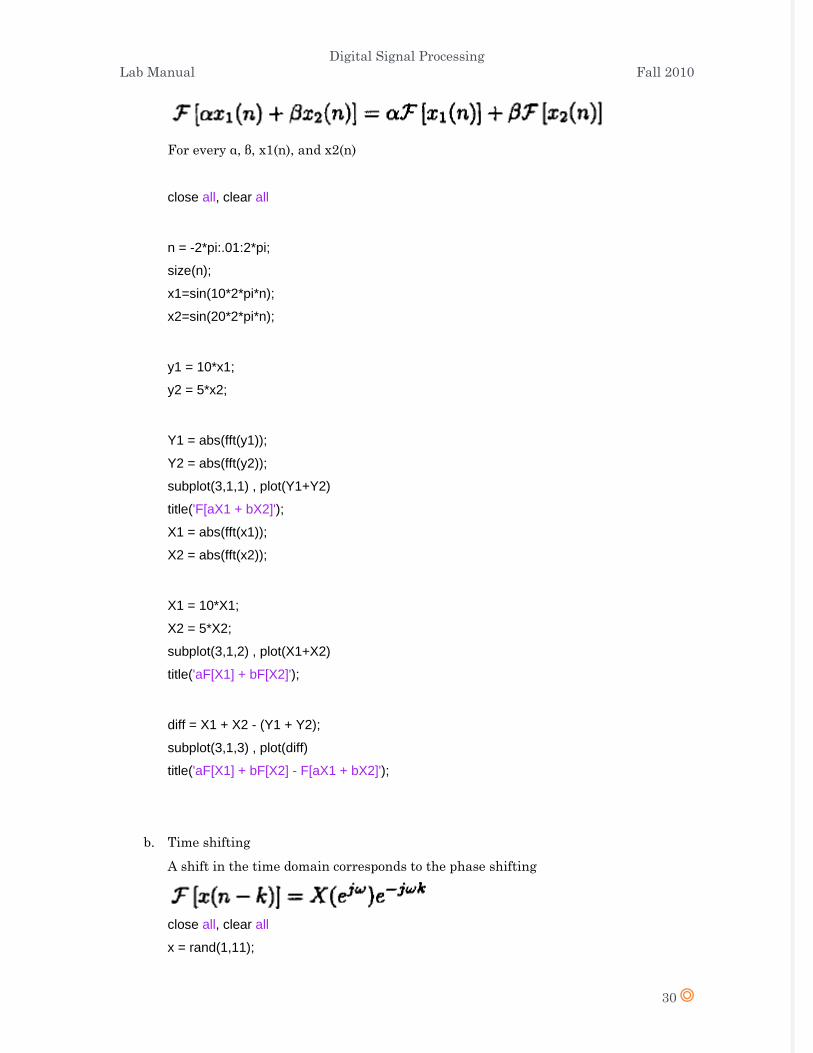
a. Linearity
The discrete-time Fourier transform is a linear transformation; that is,
Digital Signal Processing Lab Manual Fall 2010
30
For every α, β, x1(n), and x2(n)
close all, clear all n = -2*pi:.01:2*pi; size(n); x1=sin(10*2*pi*n); x2=sin(20*2*pi*n); y1 = 10*x1; y2 = 5*x2; Y1 = abs(fft(y1)); Y2 = abs(fft(y2)); subplot(3,1,1) , plot(Y1+Y2) title('F[aX1 + bX2]'); X1 = abs(fft(x1)); X2 = abs(fft(x2)); X1 = 10*X1; X2 = 5*X2; subplot(3,1,2) , plot(X1+X2) title('aF[X1] + bF[X2]'); diff = X1 + X2 - (Y1 + Y2); subplot(3,1,3) , plot(diff) title('aF[X1] + bF[X2] - F[aX1 + bX2]');
b. Time shifting
A shift in the time domain corresponds to the phase shifting
close all, clear all x = rand(1,11);
Digital Signal Processing Lab Manual Fall 2010
31
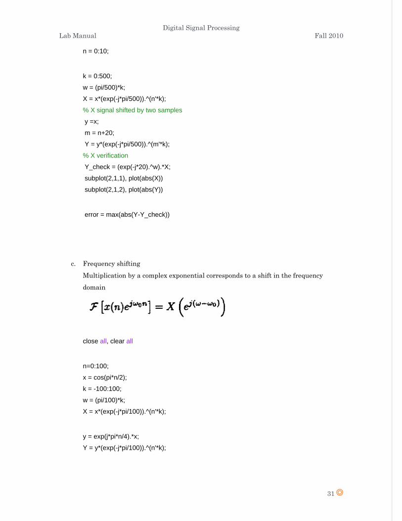
n = 0:10; k = 0:500; w = (pi/500)*k; X = x*(exp(-j*pi/500)).^(n'*k); % X signal shifted by two samples y =x; m = n+20; Y = y*(exp(-j*pi/500)).^(m'*k); % X verification Y_check = (exp(-j*20).^w).*X; subplot(2,1,1), plot(abs(X)) subplot(2,1,2), plot(abs(Y)) error = max(abs(Y-Y_check))
c. Frequency shifting
Multiplication by a complex exponential corresponds to a shift in the frequency
domain
close all, clear all n=0:100; x = cos(pi*n/2); k = -100:100; w = (pi/100)*k; X = x*(exp(-j*pi/100)).^(n'*k); y = exp(j*pi*n/4).*x; Y = y*(exp(-j*pi/100)).^(n'*k);

Digital Signal Processing Lab Manual Fall 2010
32
subplot(2,2,1) ; plot(w/pi, abs(X)); grid; axis( [-1, 1,0,60]) xlabel('frequencg in pi units'); ylabel('|X1|') title('Hagnitude of X') subplot (2,2,2) ; plot (w/pi ,angle(X)/pi); grid; axis([-1, 1, -1, 1]) xlabel('frequency in pi units'); ylabel('radiauds/pi') title('hgle of X') subplot (2,2,3) ; plot (w/pi, abs (Y)) ; grid; axis( [-1,1,0,60]) xlabel('frequency in pi units'); ylabel('|Y|') title('Magnitude of Y') subplot (2,2,4) ; plot (w/pi,angle(Y)/pi) ; grid; axis( [-1 1 -1 1]) xlabel('frequency in pi units'); ylabel('radians/pi') title('Angle of Y')
Exercise 1: Write a program which proves the convolution property described by
Excercise2: Write a program which proves the multiplication property

Digital Signal Processing Lab Manual Fall 2010
33
LAB 5: Z-TRANSFORM
Introduction
Just as the Fourier transform forms the basis of signal analysis, the z-transform forms the
basis of system analysis. If x[n] is a discrete signal, its z-transform X(z) is given by:
The z-transform maps a signal in the time domain to a power series in the complex
(frequency) domain: x[n] → X(z).
There are many advantages to working with z-transformed signals:
• linearity and superposition are preserved
• x[n − k] → z−kX(z)
• x[−n] → X(1/z)
• anx[n] → X(z/a)
• x[n] ∗ y[n] → X(z)Y (z)
The overall result is that the algebra of system analysis becomes greatly simplified in the z
domain. The only tradeoff is the necessity of taking an inverse transform to obtain time
domain responses.
Since the response y[n] of an LTI system to input x[n] is given by the convolution x[n] ∗h[n],
where h[n] is the impulse reponse, we have
The ratio H(z) = Y (z)/X(z) defines the impulse response (and so the system response), and is
called the transfer function of the system.
1. Convolution property a. If X1(Z) = 2 + 3z-1 + 4z-2 and X2(z) = 3 + 4z-1 + 5z-2 + 6z-3. Determine X3(z) = X1(z)X2(z).
clear all, close all x1 = [2,3,4]; x2 = [3 4 5 6]; x3 = conv(x1,x2) x3 =
Digital Signal Processing Lab Manual Fall 2010
34
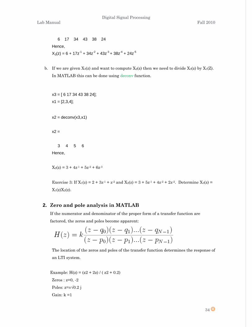
6 17 34 43 38 24
Hence,
X3(z) = 6 + 17z-1 + 34z-2 + 43z-3 + 38z-4 + 24z-5
b. If we are given X3(z) and want to compute X2(z) then we need to divide X3(z) by X1(Z).
In MATLAB this can be done using deconv function.
x3 = [ 6 17 34 43 38 24]; x1 = [2,3,4]; x2 = deconv(x3,x1)
x2 =
3 4 5 6
Hence,
X2(z) = 3 + 4z-1 + 5z-2 + 6z-3
Exercise 3: If X1(z) = 2 + 3z-1 + z-2 and X2(z) = 3 + 5z-1 + 4z-2 + 2z-2. Determine X3(z) =
X1(z)X2(z).
2. Zero and pole analysis in MATLAB If the numerator and denominator of the proper form of a transfer function are
factored, the zeros and poles become apparent:
The location of the zeros and poles of the transfer function determines the response of
an LTI system.
Example: H(z) = (z2 + 2z) / ( z2 + 0.2)
Zeros : z=0, -2
Poles: z=±√0.2 j
Gain: k =1
Digital Signal Processing Lab Manual Fall 2010
35
b = [1 2];
a = [1 0 0.2];
[z,p,k] = tf2zpk(b,a)
zplane(z,p)
3. Zero-Pole placement in Filter Design LTI systems, particularly digital filters, are often designed by positioning zeros and
poles in the z-plane. The strategy is to identify passband and stopband frequencies
on the unit circle and then position zeros and poles by cosidering the following.
i. Conjugate symmetry
All poles and zeros must be paired with their complex conjugates
ii. Causality
To ensure that the system does not depened on future values, the number of
zeros must be less than or equal to the number of poles
iii. Origin
Poles and zeros at the origin do not affect the magnitude response
iv. Stability
For a stable system, poles must be inside the unit circle. Pole radius is
proportional to the gain and inversely proportional to the bandwidth.
Passbands should contian poles near the unit circle for larger gain.
v. Minimum phase
Zeros can be placed anywhere in the z-plane. Zeros inside the uint circle
ensure minimum phase. Zeros on the unit circle give a null response.
Stopbands should contain zeros on or near the unit circle.
vi. Tranistin band
A steep transition from passband to stopband can be achieved when stopband
zeros are paired with poles along (or near) the same radial line and close to
the unit circle.
vii. Zero-pole interaction

Digital Signal Processing Lab Manual Fall 2010
36
Zeros and poles interact to produce a composite response that might not
match design goals. Poles closer to the unit circle or farther from one another
produce smaller interactions. Zeros and poles might have to be repositioned
or added, leading t a higher filter order.
Zero-Pole-Gain Editing in SPTool
Run:
Sptool
To acces the Pole/Zero Editor in SPTool, do the following:
1. Click the New button under the Filters list in SPTool.
2. Select the Pole/Zero Editor in the Algorithm list.
3. View system characteristics as you position poles and zeros.
Exercise 4: Provide examples of all seven properties mentioned above by placing
zero/poles as outlined.
4. Rational Z-transform to partial fraction form When taking inverse z-transform it is most convenient that the transfer function be
in partial fraction form. To convert from rational z-transform to partial fraction form
MATLAB residuez function can be used.
Example:
clear all, close all b = [ 0 1 0]; a = [3 -4 1]; [z,p,k] = residuez(b,a)
z =
Digital Signal Processing Lab Manual Fall 2010
37
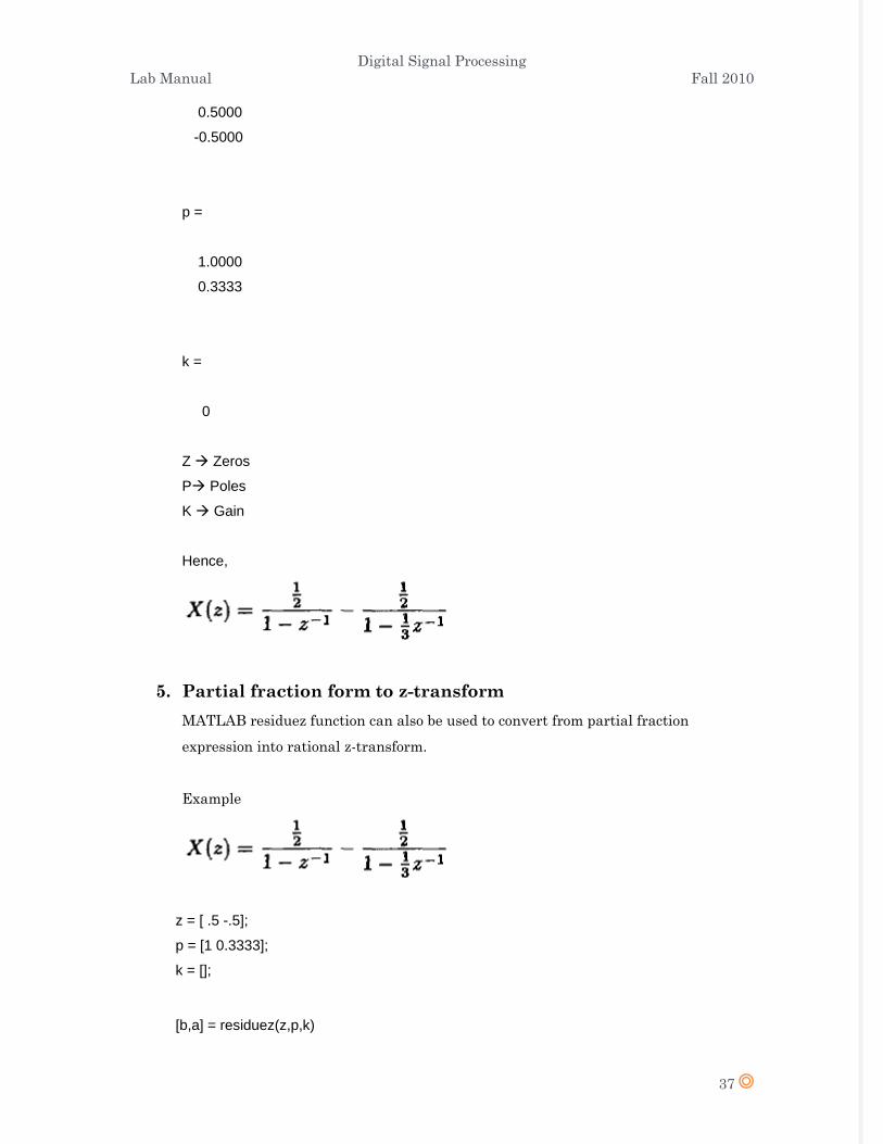
0.5000
-0.5000
p =
1.0000
0.3333
k =
0
Z Zeros
P Poles
K Gain
Hence,
5. Partial fraction form to z-transform MATLAB residuez function can also be used to convert from partial fraction
expression into rational z-transform.
Example
z = [ .5 -.5]; p = [1 0.3333]; k = []; [b,a] = residuez(z,p,k)

Digital Signal Processing Lab Manual Fall 2010
38
b =
0 0.3334
a =
1.0000 -1.3333 0.3333
Exercise 5: Determine the inverse z-transform of
Digital Signal Processing Lab Manual Fall 2010
39
LAB 6: SAMPLING, A/D CONVERSION
AND D/A CONVERSION
Introduction
Since Matlab works on a digital system, we can only simulate the sampling of a continuous
signal to produce a discrete time signal (i.e. we must approximate the continuous signal by a
discrete time signal obtained with a high sampling rate). The same comment applies for A/D
conversion and D/A conversions. But visual and audio representations of the aliasing are still
possible.
1. Time domain representation of sampling and aliasing
a. )02sin()( φπ += tftx sampled at a frequency of sf produces the discrete time signal
[ ] )02sin( φπ += nsf
fnx . Use a value of sf = 8 kHz. By varying the value of 0f , it is
possible to illustrate the aliasing. For an interval of 10 ms, plot the sampled sine wave if
0f = 300 Hz, using stem. The phase φ can be arbitrary. You should see a sinusoidal
pattern. If not, use the plot function which creates the impression of a continuous
function from discrete time values.
b. Vary the frequency 0f from 100 Hz to 475 Hz, in steps of 125 Hz. The apparent
frequency of the sinusoid should be increasing, as expected. Use subplot to put four plots
on one screen.
c. Vary the frequency 0f from 7525 Hz to 7900 Hz, in steps of 125 Hz. Note that the
apparent frequency of the sinusoid is now decreasing. Explain why.
Digital Signal Processing Lab Manual Fall 2010
40
d. Vary the frequency 0f from 32100 Hz to 32475 Hz, in steps of 125 Hz. Can you predict
in advance if the frequency will increase or decrease ? Why/How ?
2. Frequency domain representation of sampling and aliasing, A/D and D/A
convertions
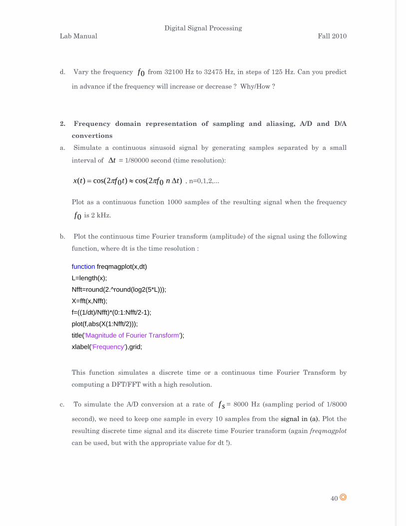
a. Simulate a continuous sinusoid signal by generating samples separated by a small
interval of t∆ = 1/80000 second (time resolution):
)02cos()02cos()( tnftftx ∆≈= ππ , n=0,1,2,...
Plot as a continuous function 1000 samples of the resulting signal when the frequency
0f is 2 kHz.
b. Plot the continuous time Fourier transform (amplitude) of the signal using the following
function, where dt is the time resolution :
function freqmagplot(x,dt) L=length(x); Nfft=round(2.^round(log2(5*L))); X=fft(x,Nfft); f=((1/dt)/Nfft)*(0:1:Nfft/2-1); plot(f,abs(X(1:Nfft/2))); title('Magnitude of Fourier Transform'); xlabel('Frequency'),grid;
This function simulates a discrete time or a continuous time Fourier Transform by
computing a DFT/FFT with a high resolution.
c. To simulate the A/D conversion at a rate of sf = 8000 Hz (sampling period of 1/8000
second), we need to keep one sample in every 10 samples from the signal in (a). Plot the
resulting discrete time signal and its discrete time Fourier transform (again freqmagplot
can be used, but with the appropriate value for dt !).
Digital Signal Processing Lab Manual Fall 2010
41
d. To simulate the D/A conversion, we need to follow two steps. In the first step, the
discrete time signal from (c) is converted to an analog pulse signal. An analog pulse
signal is the ideal case, in practice the analog signal is typically the output of a sample
and hold device. To simulate the analog pulse signal, 9 zeros are added between each
sample of the discrete time signal from (c), so that the resulting simulated continuous
signal has the original resolution of 1/80000 sec. Plot the resulting signal and its
continuous time Fourier transform.
e. The second step of the D/A conversion is to filter (interpolate) the signal found in (d), so
that the samples with zero values can be filled with non-zero values. In the frequency
domain, this means low-pass filtering the continuous Fourier transform found in (d) so
that only the first peak remains. The resulting Fourier transform should be almost
identical to the transform found in (b). To perform the low-pass filtering, use the following
filter coefficients
[b,a]=cheby2(9,60, sf *1/80000);
and the function filter. Plot the signal at the output if the filter, discard the first 200
samples (transient response) and plot the continuous time Fourier transform of the
resulting signal. Compare with (b).
f. Repeat the steps in a) b) c) d) e) with 0f = 2500 Hz, 3500 Hz, 4500 Hz, 5500 Hz (plots
not required here). When does aliasing occurs ? What is the effect of aliasing on the
output signal of the D/A converter (found in (e) ) ?

Digital Signal Processing Lab Manual Fall 2010
42
LAB 7: FIR AND IIR FILTER DESIGN IN
MATLAB
Introduction
The goal of filtering is to perform frequency-dependent alteration of a signal. A simple design
specification for a filter might be to remove noise above a certain cutoff frequency. A more
complete specification might call for a specific amount of passband ripple (Rp, in decibels),
stopband attenuation (Rs, in decibels), or transition width (Wp - Ws, in hertz). A precise
specification might ask to achieve the performance goals with the minimum filter order, call
for an arbitrary magnitude response, or require an FIR filter.
IIR filter design methods differ primarily in how performance is specified. For loosely
specified requirements, as in the first case described previously, a Butterworth filter is often
sufficient. More rigorous filter requirements can be met with Chebyshev and elliptic filters.
The Signal Processing Toolbox order selection functions estimate the minimum filter order
that meets a given set of requirements. To meet specifications with more rigid constraints,
such as linear phase or arbitrary response, it is best to use direct IIR methods such as the
Yule-Walker method or FIR methods.
Filter Configurations First, recall that when dealing with sampled signals, we can normalize the frequencies to the
Nyquist frequency, which is half the sampling frequency. All the filter design functions in the
Signal Processing Toolbox operate with normalized frequencies, so that they do not require
the system sampling rate as an extra input argument. The normalized frequency is always in
the interval 0 ≤ f ≤ 1. For example, with a 1000 Hz sampling frequency, 300 Hz is 300/500 =
0.6. To convert normalized frequency to angular frequency around the unit circle, multiply by
π. To convert normalized frequency back to Hertz, multiply by half the sample frequency.
• Lowpass filters remove high frequencies (near 1)
• Highpass filters remove low frequencies (near 0)
• Bandpass filters pass a specified range of frequencies
• Bandstop filters remove a specified range of frequencies
Digital Signal Processing Lab Manual Fall 2010
43
Calculate a normalizing factor:
fs = 1e4;
f = 400;
nf = 400/(fs/2)
Filter Specifications in Matlab
• Wp - Passband cutoff frequencies (normalized)
• Ws - Stopband cutoff frequencies (normalized)
• Rp - Passband ripple: deviation from maximum gain (dB) in the passband
• Rs - Stopband attenuation: deviation from 0 gain (dB) in the stopband
The Filter Design and Analysis Tool (FDATool) shows these specifications graphically:
fdatool
The order of the filter will increase with more stringent specifications: decreases in Rp, Rs, or
the width of the transition band.
Lab Excercises:
1. Fdatool
2. Design a Lowpass, FIR Eqiripple filter, Minimum Order, Fs=1000hz, Fpass=60,
Fstop=200, Apass 1dB, Astop 80dB. Design Filter
3. Was the filter designed as per specifications? Confirm dB at Fpass, and at Fstop.
4. Now look at the Phase Response. It is linear up to 200 hz and then there are jumps.
What size are the jumps? Are the points where the jumps occur have anything to do
with the points where the amplitude frequency response changes? (Use the icon to
look at the magnitude and phase response together). Explain the reasons for the
linear and the nonlinear behavior. Discounting the jumps, is the phase linear with
frequency?
5. Look at dφ/dω - called the group delay. What is the numerical value of this delay?
6. Look at φ/ω . Comment.
7. Look at the filter impulse response. Comment on symmetry and about what point is
it symmetric?
8. Look at i - Filter information. Note the filter length. Now how is this related to the
Group delay? Comment.
9. Look at the pole-zero plot. How many poles? How many zeros? Does this make sense?
Explain.
Digital Signal Processing Lab Manual Fall 2010
44
10. Look at filter coefficients. This is what gets implemented with varying degrees of
precision.
11. Export the filter parameters (Num) to your workspace. Do freqz(Num,1).
12. In the command window, do sptool. In sptool, Import Num to sptool. Change
sampling frequency from the default 1, to 1000.
13. Now under SPTool: startup spt, view the signal. Under Spectra, use “Create” and do
a 1024 point fft.
14. Under Options → Magnitude → Linear. Observe the difference between observing on
linear and log scales.
15. Now in fdatool, for the same specs as the first FIR filter, design an IIR Butterworth
filter. (Match exactly passband). Look at the amplitude response. Look at the phase
response. Linear phase? Look at the Filter information. Did it meet the specs? How
many poles and zeros? Look at the impulse response. Does it have any properties
dissimilar to that of the FIR filter?

Digital Signal Processing Lab Manual Fall 2010
45
LAB 8: INTRODUCTION TO TEXAS
INSTRUMENTS TMS320C6713 DSP
STARTER KIT (DSK) DIGITAL SIGNAL
PROCESSING BOARD
Introduction
Digital signal processing, or DSP, is a rapidly growing industry within Electrical and
Computer Engineering. With processing power doubling every 18 months (according to
Moore’s law), the number of applications suitable for DSP is increasing at a comparable rate.
In this course, our aim is to show how mathematical algorithms for digital signal processing
may be encoded for implementation on programmable hardware. In this first lab, you will
become familiar with a development system for programming DSP hardware. You will study:
• Code Composer Studio
• TMS320C6713 DSP chip and supporting chip set (DSK) architecture
• The C programming language
1. Hardware and Software
1.1. DSP Chip Manufacturers
Many companies produce DSP chips. Some of the more well known include Agere
Systems, Analog Devices, Motorola, Lucent Technologies, NEC, SGS-Thompson,
Conexant, and Texas Instruments. In this course, we will use DSP chips designed and
manufactured by Texas Instruments (TI). These DSP chips will be interfaced through
Code Composer Studio (CCS) software developed by TI.
1.2. Code Composer Studio (CCS)
CCS is a powerful integrated development environment that provides a useful
transition between a high-level (C or assembly) DSP program and an on-board machine
Digital Signal Processing Lab Manual Fall 2010
46
language program. CCS consists of a set of software tools and libraries for developing
DSP programs, compiling and linking them into machine code, and writing them into
memory on the DSP chip and on-board external memory. It also contains diagnostic
tools for analyzing and tracing algorithms as they are being implemented on-board. In
this class, we will always use CCS to develop, compile, and link programs that will be
downloaded from a PC to DSP hardware.
1.3. TMS320 DSP Chips
In 1983, Texas Instruments released their first generation of DSP chips, the TMS320
single-chip DSP series. The first generation chips (C1x family) could execute an
instruction in a single 200-nanosecond (ns) instruction cycle. The current generation of
TI DSPs includes the C2000, C5000, and C6000 series, which can run up to 8 32-bit
parallel instructions in one 4.44ns instruction cycle, for an instruction rate of 1.8*109
instructions per second. The C2000, and C5000 series are fixed-point processors. The
C6000 series contains both fixed point and floating-point processors. For this lab, we
will be using the C6713 processor, a member of C67x family of floating-point
processors.
The different families in the TMS320 seriea are targetted at different applications. The
C2000 and C5000 series of chips are primarily used for digital control. They consume
very little power and are used in many portable devices including 3G cell phones, GPS
(Global Positioning System) receivers, portable medical equipment, and digital music
players. Due to their low power consumption (40mW to 160mW of active power), they
are very attractive for power sensitive portable systems. The C6000 series of chips
provides both fixed and floating point processors that are used in systems that require
high performance. Since these chips are not as power efficient as the C5000 series of
chips (.5W to 1.4W of active power), they are generally not used in portable devices.
Instead, the C6000 series of chips is used in high quality digital audio applications,
broadband infrastructure, and digital video/imaging, the latter being associated almost
exclusively with the fixed-point C64x family of processors. When designing a product,
the issues of power consumption, processing power, size, reliability, efficiency, etc. will
be a concern.
Learning how to implement basic DSP algorithms on the C6713 will provide you with
the tools to execute complex designs under various constraints in future projects. At
one time, assembly language was preferred for DSP programming. Today, C is the

Digital Signal Processing Lab Manual Fall 2010
47
preferred way to code algorithms, and we shall use it for fixed- and floating-point
processing.
1.4. DSP Starter Kit (DSK)
The TMS320C6713 DSP chip is very powerful by itself, but for development of
programs, a supporting architecture is required to store programs and data, and bring
signals on and off the board. In order to use this DSP chip in a lab or development
environment, a circuit board containing appropriate components, designed and
manufactured by Spectrum Digital, Inc, is provided. Together, CCS, the DSP chip, and
supporting hardware make up the DSP Starter Kit, or DSK.
In this lab, we will go over the basic components of the DSK and show how software
may be downloaded onto the DSK.
2. Programming Languages
Assembly language was once the most commonly used programming language for DSP
chips (such as TI’s TMS320 series) and microprocessors (such as Motorola’s 68MC11
series). Coding in assembly forces the programmer to manage CPU core registers
(located on the DSP chip) and to schedule events in the CPU core. It is the most time
consuming way to program, but it is the only way to fully optimize a program.
Assembly language is specific to a given architecture and is primarily used to schedule
time critical and memory critical parts of algorithms. In this course, we will use
assembly code to gain intuition into the structure of digital filtering algorithms.
The preferred way to code algorithms is to code them in C. Coding in C requires a
compiler that will convert C code to the assembly code of a given DSP instruction set. C
compilers are very common, so this is not a limitation. In fact, it is an advantage, since
C coded algorithms may be implemented on a variety platforms (provided there is a C
compiler for a given architecture and instruction set). Most of the programs created in
this course will be coded in C. In CCS, the C compiler has four optimization levels. The
highest level of optimization will not achieve the same level of optimization that
programmer-optimized assembly programs will, but TI has done a good job in making
the optimized C compiler produce code that is comparable to programmer- optimized
assembly code.
Lastly, a cross between assembly language and C exists within CCS. It is called linear
assembly code. Linear assembly looks much like assembly language code, but it allows
for symbolic names and does not require the programmer schedule events and manage
Digital Signal Processing Lab Manual Fall 2010
48
CPU core registers on the DSP. Its advantage over C code is that it uses the DSP more
efficiently, and its advantage over assembly code is that it requires less time to
program with. This will be apparent in future labs when assembly and linear assembly
code are given.
3. Codec
The codec (coder/decoder) is a chip located on-board the DSK which interfaces the DSP
chip to the analog world, specifically signal generator(s) and either an oscilloscope or
stereo headphones.
The codec contains a coder, or analog-to-digital converter(ADC), and a decoder or
digital-to-analog converter (DAC). Both coder and decoder run at sample rates which
can be set from 8KHz to 96KHz and support data word lengths of 16b, 20b, 24b, and
32b at the digital interfaces.
4. C6713 DSP Chip
The C6713 DSP chip is a floating point processor which contains a CPU (Central
Processing Unit), internal memory, enhanced direct memory access (EDMA) controller,
and on-chip pe-ripheral interfaces. These interface include a 32-bit external memory
interface (EMIF), four Multi-channel Buffered Serial Ports (McASP and McBSP), two
32-bit timers, a host port in-terface (HPI) for high-speed communication between chips
in a multi-DSP system, an interrupt selector, and a phase lock loop (PLL), along with
hardware for ‘Boot Configurations’ and ‘Power Down Logic’.
5. Timing
The DSP chip must be able to establish communication links between the CPU (DSP
core), the codecs, and memory. The two McBSPs, serial port 0 (SP0) and serial port 1
(SP1), are used to establish bidirectional asynchronous links between the CPU and the
codec or alternately an external daughter card (not used in this course). SP0 is used to
send control data between the codec and CPU; SP1 plays a similar role for digital audio
data. The McBSPs use frame synchronization to communicate with external devices
[6]. Each McBSP has seven pins. Five of them are used for timing and the other two
are connected to the data receive and data transmit pins on the on-board codec or
daughter card. Also included in each McBSP is a 32-bit Serial Port Control Register
(SPCR). This register is updated when the on-board codec (or daughter card) is ready to
send data to or receive data from the CPU. The status of the SPCR will only be a
concern to us when polling methods are implemented.
Digital Signal Processing Lab Manual Fall 2010
49
6. Establishing a File Structure
In this section, we are going to develop a file structure on your u:\ drive that will make
imple-menting DSP algorithms easier on the DSK. Specifically, there is a set of support
files that are needed to run the DSK for every algorithm implemented in this class.
Since these files will be used many times, it will prove to be beneficial to store them in
a specific folder.
Our goal here is to create the following two paths on your u:\ drive that contain the
following types of files:
1. u:\DSP\Support { .h initialization header files, .c initialization source code files, .lib
pre-compiled binary library files, .asm vector files, and .cmd linker command file }
2. u:\DSP\Lab 07\ { .c project source code }
To create the first path, open Windows Explorer and create the folder ‘DSP’ to save
your work for this class. This folder will contain all of the sub-folders in this class. This
organization is crucial and cannot be over-stressed. Now double click on your new
folder ‘DSP’. and copy the sub-folder ‘Support’. The ‘Support’ folder contains the
following files:
c6713dskinit.c
c6713dskinit.h
dsk6713.h
dsk6713 aic23.h
dsk6713 dip.h
dsk6713 flash.h
dsk6713 led.h
csl6713.lib
dsk6713bsl.lib
rts6700.lib
Vectors intr.asm
Vectors poll.asm
c6713dsk.cmd
Now that you have these support files, go back toWindows Explorer and create another
folder: ‘Lab 07’ in the path u:\DSP\Lab 07\ Copy the file led.c into your newly created
folder ‘Lab 07’. You now have all of the support files that you will need to implement
Digital Signal Processing Lab Manual Fall 2010
50
any of the projects in this class and you also have the files required to create your first
project. At this point, you should have the following file structure established on your
u:\ drive.
1. u:\DSP\Support
c6713dskinit.c,...
2. u:\DSP\Lab 07
led.c
7. Creating the First Project on the DSK
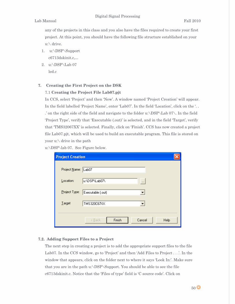
7.1 Creating the Project File Lab07.pjt
In CCS, select ‘Project’ and then ‘New’. A window named ‘Project Creation’ will appear.
In the field labelled ‘Project Name’, enter ‘Lab07’. In the field ‘Location’, click on the ‘. .
.’ on the right side of the field and navigate to the folder u:\DSP\Lab 07\. In the field
‘Project Type’, verify that ‘Executable (.out)’ is selected, and in the field ‘Target’, verify
that ‘TMS32067XX’ is selected. Finally, click on ‘Finish’. CCS has now created a project
file Lab07.pjt, which will be used to build an executable program. This file is stored on
your u:\ drive in the path
u:\DSP\lab 07. See Figure below.
7.2. Adding Support Files to a Project
The next step in creating a project is to add the appropriate support files to the file
Lab07. In the CCS window, go to ‘Project’ and then ‘Add Files to Project . . .’. In the
window that appears, click on the folder next to where it says ‘Look In:’. Make sure
that you are in the path u:\DSP\Support. You should be able to see the file
c6713dskinit.c. Notice that the ‘Files of type’ field is ‘C source code’. Click on
Digital Signal Processing Lab Manual Fall 2010
51
c6713dskinit.c and then click on ‘Open’. Re-peat this process two more times adding the
files Vectors_intr.asm and c6713dsk.cmd to the project file sine gen.pjt. For field, ‘Files
of type’, select ‘Asm Source Files (*.a*)’. Click on Vectors_intr.asm and then click on
‘Open’. For field, ‘Files of type’, select ‘Linker Command File (*.cmd)’. Click on
c6713dsk.cmd and then click on ‘Open’. You have now charged your project file
u:\DSP\Lab 07\Lab07{Lab07.pjt}.
The C source code file contains functions for initializing the DSP and peripherals. The
Vectors file contains information about what interrupts (if any) will be used and gives
the linker information about resetting the CPU. This file needs to appear in the first
block of program memory. The linker command file (c6713dsk.cmd) tells the linker how
the vectors file and the internal, external, and flash memory are to be organized in
memory. In addition, it specifies what parts of the program are to be stored in internal
memory and what parts are to be stored in the external memory. In general, the
program instructions and local/global variables will be stored in internal random access
memory or IRAM.
7.3. Adding Appropriate Libraries to a Project
In addition to the support files that you have been given, there are pre-compiled files
from TI that need to be included with your project. For this project, we need run-time
support libraries. For the C6713 DSK, there are three support libraries needed:
csl6713.lib, dsk6713bsl.lib, and rts6700.lib. The first is a chip support library, the
second a board support library, and the third is a real-time support library.
Besides the above support libraries, there is a GEL (general extension language) file
(dsk6211 6713.gel) used to initialize the DSK. The GEL file was automatically added
when the project file Lab07.pjt was created, but the other libraries must be explicitly
included in the same manner as the pre-vious files. Go to ‘Project’ and then ‘Add Files
to Project’. For ‘Files of type’, select ‘Ob-ject and Library Files (*.o*,*.l*)’. Navigate to
the path u:\DSP\Support and select the files csl6713.lib,. . . . In the left sub-window of
the CCS main window, double-click on the folder ’Libraries’ to make sure the file was
added correctly.
These files, along with our other support files, form the black box that will be required
for every project created in this class. The only files that change are the source code
files that code a DSP algorithm and possibly a vectors file.
7.4 Adding Source Code Files to a Project
Digital Signal Processing Lab Manual Fall 2010
52
The last file that you need to add to led.pjt is your C source code file. This file will
contain the code needed to control the leds through the DIP switch. Go back to ‘Project’
and then ‘Add Files to Project . . .’, but this time browse to the path u:\DSP\Lab 07.
Click on the file led.c and add it to your project by clicking on ‘Open’. You may have
noticed that the .h files cannot be added – there is no ’Files of type’ entry for .h files.
Instead, they are added in the following manner: go to ‘Project’ and select ‘Scan All
Dependencies’. In CCS, double-click on ‘led.ct’ and then double-click on ‘Include’. You
should see any header files on an #include line in your source files (including
c6713dskinit.c) plus approximately 14 other header files found by the scan step. The
latter files are supplied with the Code Composer Studio software and are used to
configure the DSP chip and board. CCS automatically found and included all needed
header files starting from the header files included in the source files. Open
c6713dskinit.c and observe that it includes c6713dskinit.h; this header and dsk6713
aic23.h (included in led.c) include other header files which in turn include others,
leading to the list observed. Note that some include files are prefixed csl ; these are chip-
support header files supplied by TI. The file dsk6713.h is a top level header file supplied
by the DSK board manufacturer, Spectrum Digital, Inc.
The project file Lab07.pjt has now been charged with all of the files required to build the
first executable .out file.
7.5. Build Options
The next objective is to customize the compiler and linker options so that the
executable file gets built correctly. Also, the compiler will first convert the C coded
programs into DSP assembly programs before it compiles them into machine code. By
selecting the appropriate options, we can keep these intermediate assembly files. For
your own amusement, you can open these files in word processing program to see how
the DSP assembly is coded.
To make these customizations, click on the ‘Project’ pull-down menu, go to ‘Build
Options’. This will open up a new window. In this window, click on the ‘Compiler’ tab.
In the ‘Category’ column, click on ‘Basic’ and select the following:
Target Version: 671x
Generate Debug Info: Full Symbolic Debug (-g)
Opt Speed vs. Size: Speed Most Critical (no ms)
Opt Level: None
Program Level Opt: None

Digital Signal Processing Lab Manual Fall 2010
53
Then click on the ‘Advanced’ entry in the ‘Category’ column and select:
Memory Models: Far
and click on the ‘Preprocessor’ entry in the ‘Category’ column and type into the boxes
the following text:
Include Search Path (-i): u:\DSP\Support
Pre-defined Symbol (-d) : CHIP_6713
In the top part of the current window, you should see:
-g -k -s -fr’’u:\dsp\lab 01\sine gen\Debug’’ -i‘‘..\..\Support’’ -d"CHIP 6713"
-mv6710 --mem model:data=far
See Figure below.
Digital Signal Processing Lab Manual Fall 2010
54
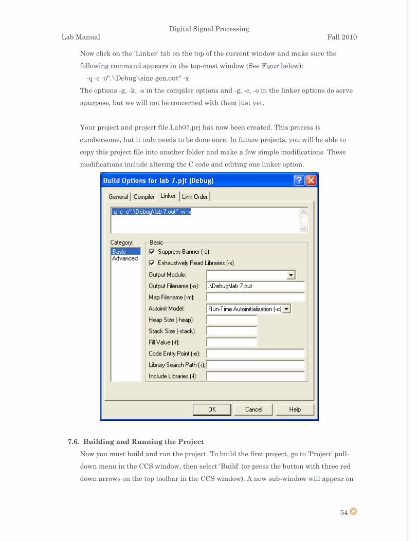
Now click on the ‘Linker’ tab on the top of the current window and make sure the
following command appears in the top-most window (See Figur below):
-q -c -o".\Debug\sine gen.out" -x
The options -g, -k, -s in the compiler options and -g, -c, -o in the linker options do serve
apurpose, but we will not be concerned with them just yet.
Your project and project file Lab07.prj has now been created. This process is
cumbersome, but it only needs to be done once. In future projects, you will be able to
copy this project file into another folder and make a few simple modifications. These
modifications include altering the C code and editing one linker option.
7.6. Building and Running the Project
Now you must build and run the project. To build the first project, go to ‘Project’ pull-
down menu in the CCS window, then select ‘Build’ (or press the button with three red
down arrows on the top toolbar in the CCS window). A new sub-window will appear on
Digital Signal Processing Lab Manual Fall 2010
55
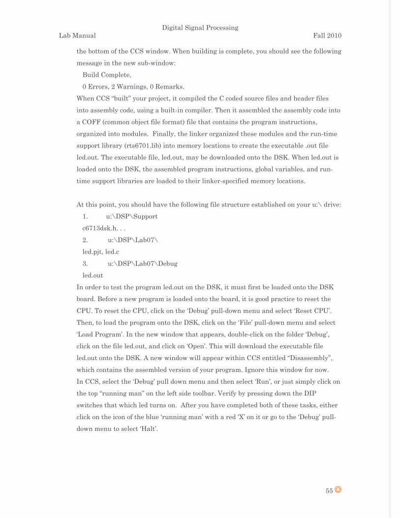
the bottom of the CCS window. When building is complete, you should see the following
message in the new sub-window:
Build Complete,
0 Errors, 2 Warnings, 0 Remarks.
When CCS “built” your project, it compiled the C coded source files and header files
into assembly code, using a built-in compiler. Then it assembled the assembly code into
a COFF (common object file format) file that contains the program instructions,
organized into modules. Finally, the linker organized these modules and the run-time
support library (rts6701.lib) into memory locations to create the executable .out file
led.out. The executable file, led.out, may be downloaded onto the DSK. When led.out is
loaded onto the DSK, the assembled program instructions, global variables, and run-
time support libraries are loaded to their linker-specified memory locations.
At this point, you should have the following file structure established on your u:\ drive:
1. u:\DSP\Support
c6713dsk.h. . .
2. u:\DSP\Lab07\
led.pjt, led.c
3. u:\DSP\Lab07\Debug
led.out
In order to test the program led.out on the DSK, it must first be loaded onto the DSK
board. Before a new program is loaded onto the board, it is good practice to reset the
CPU. To reset the CPU, click on the ‘Debug’ pull-down menu and select ‘Reset CPU’.
Then, to load the program onto the DSK, click on the ‘File’ pull-down menu and select
‘Load Program’. In the new window that appears, double-click on the folder ‘Debug’,
click on the file led.out, and click on ‘Open’. This will download the executable file
led.out onto the DSK. A new window will appear within CCS entitled “Disassembly”,
which contains the assembled version of your program. Ignore this window for now.
In CCS, select the ‘Debug’ pull down menu and then select ‘Run’, or just simply click on
the top “running man” on the left side toolbar. Verify by pressing down the DIP
switches that which led turns on. After you have completed both of these tasks, either
click on the icon of the blue ‘running man’ with a red ‘X’ on it or go to the ‘Debug’ pull-
down menu to select ‘Halt’.

Digital Signal Processing Lab Manual Fall 2010
56
LAB 9: INTERRUPTS AND
VISUALIZATION TOOLS
Introduction
In this laboratory you will use hardware and software interrupts in the C6713. You will also
use visualization tools available in the CCS. You will also learn to interface C6713 with
MATLAB where you will be able to use visualization tools in MATLAB through audio
interfacing the DSK with your PC.
1. Interrupts and Visualization in the CCS
In the interrupt mode, an interrupt stops the current CPU process to that it can perform
a required task initiated by an interrupt, and it is redirected to an interrupt service
routine (ISR).
Create this project as lab8.pjt in a new directory lab8 , and add the necessary files to the
project, as in Lab 07 (use the C source program sine8_buf.c in lieu of led.c). Note that the
necessary header support files are added to the project by selecting Project Scan All
File Dependencies. The necessary support files for this project, c6713dskinit.c,
vectors_intr.asm and C6713dsk.cmd, are in the folder support. Also add the appropriate
libraries csl6713.lb, dsk6713bsl.lib, and rts6700.lib. Add the source file sine8_buf.c to the
project. Apply the build options as done in lab 07. After completing the above Build the
the project from Project Build drop down menus.
Connect the c6713 and then load the sine8_buf.out. Run the project from Debug Run.
1.1. Plotting with the CCS
The output buffer is being updated continuously every 256 points (you can readily
change the buffer size). Use CCS to plot the current output data stored in the buffer
out_buffer.

Digital Signal Processing Lab Manual Fall 2010
57
a. Select View Graph Time/Frequency. Change the Graph Property Dialog so that the
options in Figure 1 are selected for a time-domain plot (use the pull-down menu when
appropriate).The starting address of the output buffer is out_buffer. The other options
can be left as default. Figure 3 shows a time-domain plot of the sinusoidal signal within
CCS.
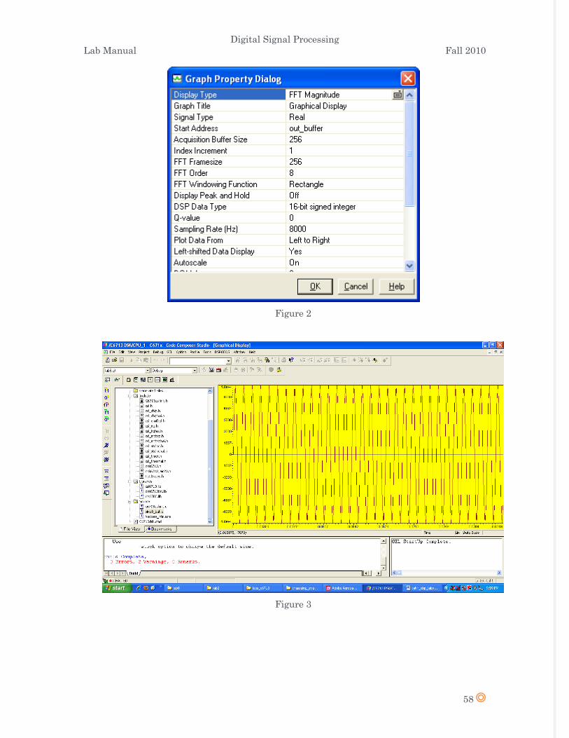
b. Figure 2 shows CCS’s Graph Property Display for a frequency-domain plot. Choose a
fast Fourier transform (FFT) order so that the frame size is 2order. Press OK and verify
that the FFT magnitude plot is as shown in Figure 4. The spike at 1000 Hz represents
the frequency of the sinusoid generated.
Figure 1
Digital Signal Processing Lab Manual Fall 2010
58
Figure 2
Figure 3

Digital Signal Processing Lab Manual Fall 2010
59
Figure 4
1.2. Plotting with MATLAB
Run MATLAB and open Simulink Library Browser by clicking the icon as shown below.
Figure 5
In the Simulink Library Browser create a new model from File New Model. In the
new model window create the following model.

Digital Signal Processing Lab Manual Fall 2010
60
Figure 6
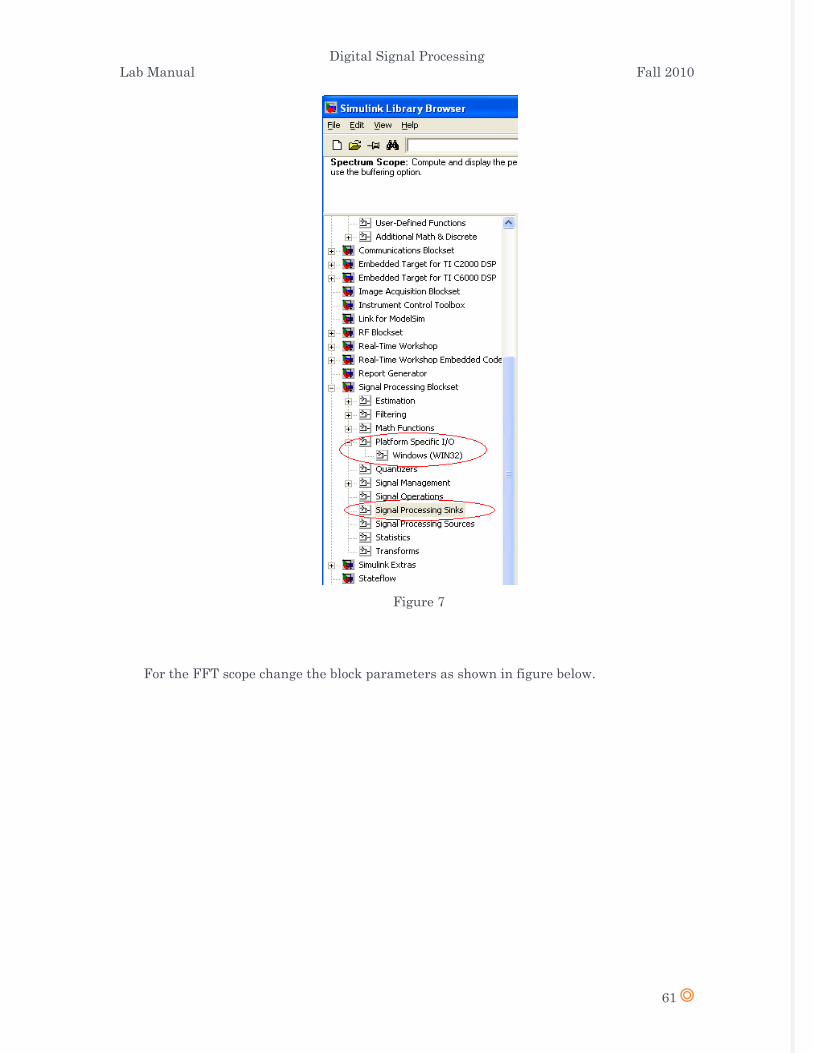
The Blocks can be found under the Signal Processing Blockset.
Digital Signal Processing Lab Manual Fall 2010
61
Figure 7
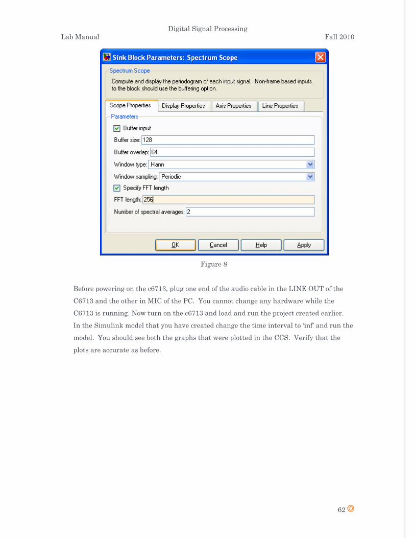
For the FFT scope change the block parameters as shown in figure below.
Digital Signal Processing Lab Manual Fall 2010
62
Figure 8
Before powering on the c6713, plug one end of the audio cable in the LINE OUT of the
C6713 and the other in MIC of the PC. You cannot change any hardware while the
C6713 is running. Now turn on the c6713 and load and run the project created earlier.
In the Simulink model that you have created change the time interval to ‘inf’ and run the
model. You should see both the graphs that were plotted in the CCS. Verify that the
plots are accurate as before.

Digital Signal Processing Lab Manual Fall 2010
63
LAB 10: SAMPLING IN CCS AND C6713
Introduction
In this laboratory you will learn to configure sampling rate in CCS. Lab will also go
through signal generation using lookup tables. A table is created via MATLAB with
the values of sine wave. The sampling frequency that is set in CCS is used to
generate the table in MATLAB.
1. Open and run the tone.pjt project located at
C:\CCStudio_v3.1\examples\dsk6713\bsl\tone
2. The frequency of the signal is 1KHz. Change this frequency to 2KHz.
Hint: Use MATLAB to get a signal of 2 KHz and use its value.
3. Now, change the frequency to 3 KHz.
4. This time change the frequency to 4 KHz. What do you notice?
5. Change the sampling frequency to 48 KHz. The following instruction can be
used to change the frequency of the codec.
DSK6713_AIC23_setFreq(hAIC23_handle, DSK6713_AIC23_FREQ_48KHZ);
You will have to obtain a new lookup table for 1 KHz signal from MATLAB.
Digital Signal Processing Lab Manual Fall 2010
64
LAB 11: FIR FILTER DESIGN IN CCS
Introduction
In this laboratory you will design FIR filters and will learn more about the capabilities of the
C6713. Filtering is one of the most useful signal processing operations. DSPs are now
available to implement digital filters in real time. A FIR filter operates on discrete-time
signals and can be implemented on a DSP such as the TMS320C6x. This process involves the
use of an ADC to acquire an external input signal, processing of the samples, and sending
the result through a DAC. Filter characteristics such as center frequency, bandwidth, and
filter type can be readily implemented and modified.
Lab Excercises:
1. Open and run the FIR project
2. There are four different filter coefficients saved in four *.dat files. Provide
the time and frequency plots for each.
3. Apply a signal from MATLAB and show the effect on the signal after it
passes through the filter(s).
Digital Signal Processing Lab Manual Fall 2010
65
LAB 12: IIR FILTER DESIGN IN CCS
Introduction
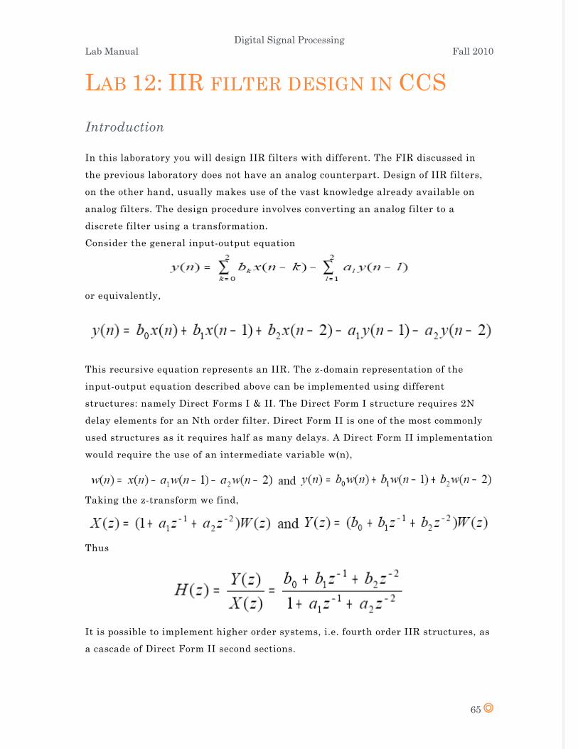
In this laboratory you will design IIR filters with different. The FIR discussed in
the previous laboratory does not have an analog counterpart. Design of IIR filters,
on the other hand, usually makes use of the vast knowledge already available on
analog filters. The design procedure involves converting an analog filter to a
discrete filter using a transformation.
Consider the general input-output equation
or equivalently,
This recursive equation represents an IIR. The z-domain representation of the
input-output equation described above can be implemented using different
structures: namely Direct Forms I & II. The Direct Form I structure requires 2N
delay elements for an Nth order filter. Direct Form II is one of the most commonly
used structures as it requires half as many delays. A Direct Form II implementation
would require the use of an intermediate variable w(n),
Taking the z-transform we find,
Thus
It is possible to implement higher order systems, i.e. fourth order IIR structures, as
a cascade of Direct Form II second sections.

Digital Signal Processing Lab Manual Fall 2010
66
Lab Excercises:
1. Open and run the IIR project
2. There are four different filter coefficients saved in four *.dat files. Provide
the time and frequency plots for each.
3. Apply a signal from MATLAB and show the effect on the signal after it
passes through the filter(s).


