+ All Categories
Home > Documents > Teaching Dynamic Aggregate Supply-Aggregate Demand Model ...

Teaching Dynamic Aggregate Supply-Aggregate Demand Model ...

Date post: 23-Mar-2022
Category:
Upload: others
View: 2 times
Download: 0 times
Share this document with a friend
15
Teaching Dynamic Aggregate Supply-Aggregate Demand Model in an Intermediate Macroeconomics Class Using Interactive Spreadsheets Sarah Ghosh (E-Mail: [email protected]) Satyajit Ghosh (E-Mail: [email protected]) Department of Economics and Finance University of Scranton AEA/ASSA Conference, Chicago, January, 2012 Preliminary draft: not to be quoted without written permission of the authors.
Transcript

Teaching Dynamic Aggregate Supply-Aggregate Demand Model in an

Intermediate Macroeconomics Class Using Interactive Spreadsheets

Sarah Ghosh

(E-Mail: [email protected])

Satyajit Ghosh

(E-Mail: [email protected])

Department of Economics and Finance

University of Scranton

AEA/ASSA Conference, Chicago, January, 2012

Preliminary draft: not to be quoted without written permission of the authors.

2

Abstract

In our intermediate macroeconomics class in order to initiate student interest we introduce the aggregate

supply-aggregate demand models using spreadsheet based interactive graphs. Although we use Excel in

our classrooms, we have developed the same framework using ―Calc‖. Our goal is to engage students in

using aggregate supply-aggregate demand models to analyze the impacts of demand and supply shocks

by focusing on adjustments over time which are based on price or inflation expectations. We use two

models: model 1 is a traditional AS-AD model where updating of price expectations is the key for

economic adjustment; model 2 uses the monetary policy rule to derive the (dynamic) aggregate demand

curve (DAD) and the Phillips curve to derive the (dynamic) aggregate supply curve (DAS). Here the

dynamic adjustment is brought about by updating of expected inflation. To create interactive graphs that

students can control we insert ―scrollbars‖ and ―spin buttons‖ from Excel’s toolbar (accessible from the

Developer tab in 2007 Excel) on a work sheet that contains the AS-AD or DAD-DAS models. The

scrollbars are linked to price or inflation expectations and demand parameters. Spin buttons are linked to

demand and supply shocks. Students can move the slider of the scrollbars to the right or to the left to

change the values of expected price or inflation. They can also adjust the parameters of the monetary

policy rule that affect the DAD curve. The spin buttons give them the control of demand and supply

shocks. For each model, following a shock students adjust expected price or inflation and control the

shifts of the aggregate supply curves. Although for illustration we use adaptive expectation, the interactive

graphs are flexible to handle other expectation formation mechanisms. Students can alter the parameters

of the monetary policy rule and the DAD curve and observe their impacts on the effects of shocks. The

entire exercise becomes totally dynamic and interactive and students maintain complete control of their

learning process. They remain engaged and become better motivated and prepared for analytical

discussions of dynamic adjustments.

3

Teaching Dynamic Aggregate Supply-Aggregate Demand Model in an Intermediate

Macroeconomics Class Using Interactive Spreadsheets

1. Introduction

Almost every economics instructor wants their students to ―think like an economist‖. It is one of

the most overused phrases in undergraduate economics syllabi, but represents a laudable goal.

While an economist may not have any more or any less claim to be a critical thinker than a

physicist, a mathematician or a sociologist, to ―think like an economist‖ implies the ability to think

critically using sound economic principles. Students will be able to think like economists only if

they understand underlying economic concepts clearly and also can successfully use them in

analytical thinking and problem solving. The hardest part of economics instruction can be finding

the right method of teaching that will engage the students, grab their attention and ultimately

involve them in learning something new and exciting. There are many who argue that if students

can be successfully involved in the process of learning, the outcome will definitely be more

promising.

There can be many possible methods of classroom teaching that ensure active involvement on

the part of the student. Schmidt (2003) noted, ―During the last 10-15 years economists have

turned increasingly to the use of simulation exercises as a way to introduce active and

cooperative learning in their courses.‖ In this paper we discuss how we have used a visual

interface of spreadsheet applications to develop simulations to analyze dynamic adjustments in

aggregate supply-aggregate demand models and how we have integrated such simulations in

our teaching.

The plan of the paper is as follows. In the following section we discuss in general the concept of

active learning and the obstacles to incorporate active learning strategies such as simulations in

a classroom. In section 3, we discuss in detail how we have developed two spreadsheet based

simulation models for use in intermediate level microeconomics courses. Concluding remarks

are made in section 4.

2. Active Learning: Promise and Obstacles

In spite of frequent use of the term ―active learning‖ there is no universally accepted definition of

active learning. Instead of a precise definition, active learning is often described by certain

features of the process of learning. At the heart of the description of active learning is the notion

that ― active learning is more likely to take place when students are doing something besides

listening‖ (Ryan and Martens, 1989).Bonwell and Eison (1991) list the general characteristics of

active learning strategies. They include the following:

Students are involved in more than listening.

Students are involved in higher-order thinking (analysis, synthesis, evaluation).

Students are engaged in activities.

4

Based on these characteristics of active learning strategies, Bonwell and Eison propose the

following working definition of active learning: active learning ―involves students in doing things

and thinking about the things that they are doing.‖

While there may not be a universally accepted precise definition of active learning, the

importance and benefits of active learning cannot be overstated. Chickering and Gamson

(1987) proclaim, ―learning is not a spectator sport. Students do not learn much just by sitting in

class listening to teachers….They must make what they learn part of themselves.‖ Cross (1987)

goes a step further and argues that ―when students are actively involved in learning, they learn

more than when they are passive recipients of instruction.‖ It is now generally accepted that

active learning, however clumsily it may be defined, significantly enhances student learning.

While in general a college faculty may appreciate the benefits of active learning strategies, there

is still a great deal of hesitation among faculty in incorporating active learning strategies in their

classroom teaching. Bonwell and Eison list some of the barriers to the use of active learning

strategies. Faculty members often refrain from using active learning strategies because they

feel that (i) incorporation of active learning strategies may reduce coverage of content, (ii) it is

too time consuming to develop appropriate active learning strategies and, (iii) it may not be

possible to promote active learning strategies in large classes.

But perhaps the biggest obstacle to the use of active learning strategies is the perception of two

types of risks associated with such learning strategies. The first type of risk is that students may

not participate in the ―activities‖ and consequently, instead of taking charge of their own

learning, they will be more disengaged. The second type of risk that the faculty often is fearful of

is that active learning strategies may not be readily integrated with their existing teaching

strategy and as a result students will not learn as much.

Simulations have long been viewed as a very effective active learning tool. Some twenty-five

years back Day (1987) discussed the use of simulation models in the classroom and Scheraga

(1986) argued that instruction through simulated programming can motivate ― the student to

think for herself and to think like an economist‖. But in spite of the recognition of the importance

of active learning approach and the growing interest in simulation as an effective active learning

model, it is somewhat disappointing to note that ―educators still use these practices in

undergraduate economics courses relatively infrequently‖ and that ―computer labs and computer

games and simulations are almost never used to teach economics‖. (Watts and Becker, 2008)

We now turn to the two spreadsheet based simulation models that we have developed and used

to teach dynamic adjustments in aggregate supply-aggregate demand models in our

intermediate macroeconomics course.

5

3. Two Examples of Dynamic Adjustment Simulations in Aggregate Supply-

Aggregate Demand Models.

Aggregate supply-aggregate demand (AS-AD) model plays a crucial role in an Intermediate

macroeconomics course. It is used to analyze the effects of demand and supply shocks, explain

the working of macroeconomic policies but perhaps most importantly, to demonstrate the

economic adjustments over time. In an intermediate macroeconomics class students need to

understand the analytical concepts with the help of graphical expositions. However, they often

find the graphical analysis of the AS-AD model difficult to understand, let alone use them

appropriately to analyze the dynamic adjustments in the economy or evaluate the effectiveness

of fiscal and monetary policies. Admittedly, the graphs for the AS-AD model, in particular the

shifts of the curves that are at the heart of analyzing the adjustments of the economy developed

are somewhat complex. Students often find them difficult to understand and fail to follow the

analysis as presented in the text or in a regular class lecture.

In our Intermediate Macroeconomics class we have developed an active learning framework to

teach the working of the AS-AD models. We use a visual interface of spreadsheet applications

to develop interactive graphs. Students themselves control the graphs and thus create

numerous graphical combinations to aid their understanding.

We present these materials using Excel spreadsheets. Since students and faculty are usually

very familiar with Excel, the navigation of the spreadsheet and the minimal programming that is

needed to make the spreadsheets interactive, are not likely to pose any great difficulty for

students and faculty and they can focus on the economic content of the subject matter.

Although we use Excel in our classrooms, these exercises can be presented using ―Calc‖ of the

popular open-source software, ―Open Office.‖ We usually hold these classes in computer labs or

classrooms that are equipped with laptops. However, the student activities required in these

models can also be assigned as home works without diminishing their value as active learning

tools.

We develop two dynamic aggregate supply – aggregate demand simulation models. Model 1 is

the traditional AS-AD model where the AS and AD curves show the relationships between real

GDP, Y and the price level P. Dynamic adjustments work through updating of expected price

level Pe. While the aggregate supply curve is a variant of the Phillips curve, the aggregate

demand curve is usually derived from an IS-LM framework ( Blanchard (2011)). Model 2 is

based on the relationship between GDP and rate of inflation, . Dynamic adjustments work

through updating of expected inflation . Here the aggregate supply curve is nothing but the

Phillips curve, but the aggregate demand relationship is based on an explicit monetary policy

rule (Mankiw 2010).

6

Model 1: Traditional AS-AD Model

In order to develop an interactive AS-AD model we start with the following linear model:

Aggregate Supply (AS): Yt = Yn + c(Pt – Pt e), c>0 (1)

Aggregate Demand (AD): Yt = a-bPt, a, b >0 (2)

Adaptive Expectations: Pt e = Pt-1 (3)

where Yn denotes the natural rate of output and Pte the price level expected to prevail in period t.

For the purpose of our simulation we parameterize the above AS-AD model with the following

baseline model:

AD: Yt = 550 – 50Pt (4)

AS: Yt = 400+ 50 (Pt –Pte) (5)

and, Yn = 400 (6)

The purpose of this simulation is to demonstrate how the economy adjusts following a demand

shock. We begin by drawing the graphs of the above aggregate demand and aggregate supply

curves using Excel’s chart drawing tool. As shown in figure 1, initially the economy is at long run

full employment equilibrium with real GDP at the natural rate of output of 400 and P = Pe=3.

As the first step of our simulation we need to demonstrate how a demand shock affects the AS-

AD model. To accomplish this, we insert on our worksheet a ―spin button‖ from Excel’s toolbar

(accessible from the Developer tab in 2007 excel or the View tab in 2003 excel). Using the

linked cell property under the format control for the spin button we link cell I4 to the value of the

spin button that controls the direction as well as the magnitude of the demand shock. By

pressing the up or down arrow on the spin button, students can choose the demand shock.

Figure 1 shows the impact of a positive demand shock of 100. When students generate a

positive demand shock of 100, the AD curve shifts to the right and as shown on the worksheet

and the accompanying diagram real GDP increases to 450 and the price level rises to $4. But

there is no immediate adjustment of expected price.

We now focus on the economic adjustment that follows the demand shock. Since this is brought

about by updating of price expectation that causes the aggregate supply curve to shift, we insert

a ―scrollbar‖ on our worksheet. Just as the spin button, the scrollbar is also accessible from the

Developer tab in 2007 Excel or the View tab in 2003 Excel. The function of the scrollbar is to

control the adjustment of the expected price level, Pe .Using the format control of the scrollbar

we set the range of values of the scrollbar slider between 0 and 6 with an increment of .05. We

use the linked cell property of the scrollbar to link it to cell N4. Thus the value in cell N4 shows

the expected price level which students can control by moving the scrollbar slider. A rightward

7

Figure 1

8

movement of the scrollbar slider raises the value of the expected price level, while a leftward

movement reduces it.

As shown in figure 1, the demand shock creates a positive output gap and a mismatch between

the actual price level and the expected price level. At this point the expected price level needs to

be updated. We can now update the expected price level following the adaptive price

expectation rule shown in equation 3. As illustrated in Figure 2, Students can move the

scrollbar slider to the right to raise expected price to the level of the current price of $4. It should

be emphasized that although we use adaptive expectation formation for illustrating the

simulation, the simulation model can handle any type of price expectation. The updating of

expected price level triggers a change in the AS-AD model. As shown in Figure 2, it leads to an

upward shift of the AS curve. A new equilibrium is reached at Y = 425 and the price level

increases further to P = 4.25. The positive output gap and a mismatch between the actual and

expected price level necessitate further updating of expected price level. Students can continue

to adjust the expected price level by moving the control of the scrollbar. The AS curve continues

to shift up and leftward. The process of economic adjustment comes to an end when the

economy returns to a long run full employment equilibrium at Y = Yn = 400 and with P = Pe =$5.

Figure 2

9

Model2: Dynamic Aggregate Supply-Dynamic Aggregate Demand Model with Monetary

Policy Rule

This variation of the aggregate supply-aggregate demand model focuses on the relationship

between real GDP and inflation and incorporates a monetary policy rule (Taylor rule). Following

Mankiw (2010) we will refer to this model as the DAS-DAD model. It is based on the following

relationships.

Phillips Curve: πt = πte + σ(Yt – Yn), σ>0 (7)

Demand for Goods and Services: Yt = Yn –β(rt – rn), β>0 (8)

Fisher Equation: rt = it - πt+1e (9)

Monetary Policy Rule: it = πt + rn + θ1(πt – π*) + θ2(Yt – Yn), θ1, θ2 >0 (10)

Adaptive Expectations: πte = πt-1 (11)

where πte is the inflation rate expected to prevail in period t, rt the real rate of interest, rn the

natural real rate of interest, i.e., the rate of interest when the real GDP Y is at the natural rate of

output, Yn in the absence of any shock, it is the nominal rate of interest or the federal funds rate

set by the Fed, π*the target rate of inflation and θ1, θ2 are the weights assigned by the Fed to

the inflation gap and the output gap in the monetary policy rule.

We can rewrite (7) as the following DAS (Dynamic Aggregate Supply) equation:

DAS: Yt = Yn +φ(πt - πte), φ >0 (12)

Substituting (9), (11) and (10) in (8) we can derive the equation for the DAD (Dynamic

Aggregate Demand) curve:

DAD: Yt = Yn – α(πt – π*) (13)

where α = [βθ1/(1+ βθ2)]>0

(For details of the derivation of DAD see Mankiw)

For the purpose of our simulation we parameterize the above DAS-DAD model with the

following baseline model:

DAS: Yt = 50 + 2(πt - πte) (14)

DAD: Yt = 50 - .5(πt -2) (15)

where Yn = 50 and π*=2 (percentage point).

10

The purpose of this simulation is to demonstrate how the economy adjusts following a supply

shock. We begin by drawing the graphs of the above DAS and DAD curves using Excel’s chart

drawing tool. As shown in figure 3, initially the economy is at long run full employment

equilibrium with real GDP at the natural rate of output of 50 and π = π*= πe = 2%. Initially, the

nominal interest rate, i = 4%, while the real rate of interest is at the natural raate level, r = rn =

2%.

As in the simulation for model 1 we insert a ―spin button‖ on our worksheet. The linked cell I4

shows the direction as well as the magnitude of the supply shock that is controlled by the spin

button. Figure 3 shows the impact of an adverse supply (inflation) shock of 2.5 percentage

point. When students generate such an adverse supply shock, the DAS curve shifts up and as

shown on the worksheet and the accompanying diagram real GDP falls to 49 and the inflation

rate rises to 4%. Furthermore, the nominal and the real rates of interest both increase—the

nominal rate increasing to 6.5% and the real rate increasing to 2.5%.

We now focus on the economic adjustment that follows the supply shock. Since the adjustment

is triggered by changes in expected inflation rate that cause further shifts of the DAS curve, we

insert a ―scrollbar‖ on our worksheet that controls expected inflation. Using the format control of

the scrollbar we set the range of values of the scrollbar slider between 0 and 6% with an

increment of .01%. We use the linked cell property of the scrollbar to link it to cell N4. Thus the

value in cell N4 shows the expected inflation rate which students can control by moving the

scrollbar slider.

As shown in figure 3, the supply shock creates a negative output gap. But it also creates a

mismatch between the actual and the expected inflation rates. As the DAS curve shifts up due

to an exogenous supply shock, individual workers and firms should have expected an increase

in inflation by the full amount of the supply shock. But instead of an inflation rate of (2+2.5) or

4.5 percentage point, following the supply shock, inflation is seen to increase only to 4%. The

less than full increase in inflation rate can be attributed to the central bank’s automatic

adjustment of the nominal interest rate, which influences the slope of the demand curve. Since

there is a mismatch between the actual and the expected inflation rates, individuals update their

expectations. As for model 1 simulation, we use adaptive expectations rule, shown in equation

(11) for updating expectations, but the simulation can handle any other type of expectation

formation. As illustrated in Figure 4, following the adaptive expectations rule, students move the

scrollbar slider to change expected inflation to 4%--the current inflation rate. Since a 4.5%

inflation could be expected in the absence of the central bank’s automatic policy adjustment, the

change in expected inflation is construed as a downward revision of expected inflation.

Consequently, the DAS curve shifts down and to the right to a new GDP of 49.2, thereby

reducing the size of the negative output gap. Nominal interest rate falls to 6%, while the real rate

of interest falls to 2.4%. The inflation rate falls to 3.6%. The negative output gap and a mismatch

between the actual and expected price level necessitate further updating of expected inflation.

Students can continue to adjust expected inflation rate by moving the control of the scrollbar.

The DAS curve continues to shift down until the economy returns to the initial long run

equilibrium with Y = Yn = 50, π = π*= 2%, i = 4% and r = rn = 2%.

11

Figure 3

12

Figure 4

We finally consider the effects of Fed’s policy changes that influence the DAD curve. As per our

formulation of the monetary policy rule, there are three policy parameters of interest: θ1, the weight for inflation adjustment, i.e., the responsiveness of the Fed to inflation’s deviation from its

target, θ2, weight for output gap, i.e., the responsiveness of the Fed to the output gap and π*,

the target rate of inflation. As it is evident from our discussion of the DAD curve (13) and its

slope, changes in any of these parameters affect the DAD curve and consequently influence the

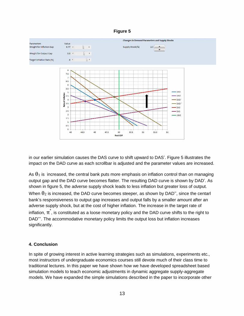
impact of a shock. Figure 5 illustrates the effects of the changes in these parameters on the

DAD curve and the resulting impact of an adverse supply shock.

In order to examine the impacts of these parameter changes we incorporate three scrollbars on

our worksheet. Each scrollbar controls one of the three parameters. For the purpose of these

simulations we use the same baseline model for the monetary policy rule that we have used for

the baseline model for the DAD curve of equation (15). Specifically, the baseline for the

monetary policy rule of (10) is given by:

it = 2 + rn + .5(πt – 2) + .5(Yt – 50) (16)

Using the format control we set the ranges for θ1 and θ2 from .1 to 1 with an increment of .01

and the range for π* from 1 to 4 percentage point with an increment of .1. As with all other

scrollbars the sliders control the values of the linked parameter. In figure 5 we begin with the

initial baseline DAD curve and the DAS curve. As before they intersect at the longrun

equilibrium position with Y = Yn = 50, π = π*= 2%. The adverse supply shock as described

13

Figure 5

in our earlier simulation causes the DAS curve to shift upward to DAS’. Figure 5 illustrates the

impact on the DAD curve as each scrollbar is adjusted and the parameter values are increased.

As θ1 is increased, the central bank puts more emphasis on inflation control than on managing

output gap and the DAD curve becomes flatter. The resulting DAD curve is shown by DAD’. As

shown in figure 5, the adverse supply shock leads to less inflation but greater loss of output.

When θ2 is increased, the DAD curve becomes steeper, as shown by DAD’’, since the centarl

bank’s responsiveness to output gap increases and output falls by a smaller amount after an

adverse supply shock, but at the cost of higher inflation. The increase in the target rate of

inflation, π*, is constituted as a loose monetary policy and the DAD curve shifts to the right to

DAD’’’. The accommodative monetary policy limits the output loss but inflation increases

significantly.

4. Conclusion

In spite of growing interest in active learning strategies such as simulations, experiments etc.,

most instructors of undergraduate economics courses still devote much of their class time to

traditional lectures. In this paper we have shown how we have developed spreadsheet based

simulation models to teach economic adjustments in dynamic aggregate supply-aggregate

models. We have expanded the simple simulations described in the paper to incorporate other

14

expectation forming structures as well as active policies following the demand and supply

shocks.

Furthermore, since instructors and students are familiar with Excel spreadsheets, these

simulations can be further expanded and modified by instructors to suit their needs. Thus, these

spreadsheet based simulations can be easily integrated with alternative teaching styles. We

usually assign the simulations to students as class assignments or even as home works before

we discuss the topics rigorously in class. We have found that since students actively control the

models and generate the graphs, they become more interested in the topic and generally retain

the material better. Once they understand the mechanics of the graphs by working through the

simulations, we can spend more time in class discussing the economic principles underlying

these models. We plan to discuss the assessment results of these and other simulations that we

have used in a future paper.

15

References

Blanchard,O. (2011).Macroeconomics, 5th. ed (updated),Prentice Hall, Boston, MA.

Bonwell, C.C. and Eison, J.A. (1991). Active Learning: Creating excitement in the classroom.

ERIC Clearinghouse on Higher Education. The George Washington University, Washington

D.C.

Chickering, A.W. and Gamson, Z.F. (1987). Seven principles for good practice. AAHE Bulletin

39:3-7.

Cross, P.K. (1987). Teaching for learning. AAHE Bulletin 39:3-7.

Day,E. (1987). A note on simulation models in the Economics classroom. Journal of Economic

Education, 351-356.

Mankiw, N.G. (2010). Macroeconomics, 7th. ed., Worth Publishers, New York, NY.

Ryan, M.P., and Martens, G.G. (1989). Planning a college course: A guidebook for the graduate

teaching assistant. National Center for Research to Improve Postsecondary Teaching and

Learning. Ann Arbor, MI.

Scheraga, J.D. (1986). Instruction in Economics through simulated computer programming.

Journal of Economic Education, 129-139.

Schmidt, S.J. (2003). Active and cooperative learning using web-based simulations.Journal of

Economic Education, 151-167.

Watts, M. and Becker, W.E. (2008). A little more than chalk and talk: Results from a third

national survey of teaching methods in undergraduate Economics courses. Journal of Economic

Education, 273-86.


Recommended