P. Quaresma and W. Neuper (Eds.): 6th International Workshopon Theorem proving components for Educational software (ThEdu’17)EPTCS 267, 2018, pp. 120–139, doi:10.4204/EPTCS.267.8

c© W. Schreiner, A. Brunhuemer & C. FürstThis work is licensed under theCreative Commons Attribution License.

Teaching the Formalization of Mathematical Theories andAlgorithms via the Automatic Checking of Finite Models∗

Wolfgang Schreiner Alexander Brunhuemer Christoph FürstResearch Institute for Symbolic Computation (RISC) & Linz Institute of Technology (LIT)

Johannes Kepler University, Linz, AustriaWolfgang.Schreiner@risc.jku.at alex.brunhuemer@gmail.com Christoph.Fuerst@risc.jku.at

Education in the practical applications of logic and proving such as the formal specification andverification of computer programs is substantially hampered by the fact that most time and effortthat is invested in proving is actually wasted in vain: because of errors in the specifications respec-tively algorithms that students have developed, their proof attempts are often pointless (because theproposition proved is actually not of interest) or a priori doomed to fail (because the proposition to beproved does actually not hold); this is a frequent source of frustration and gives formal methods a badreputation. RISCAL (RISC Algorithm Language) is a formal specification language and associatedsoftware system that attempts to overcome this problem by making logic formalization fun ratherthan a burden. To this end, RISCAL allows students to easily validate the correctness of instancesof propositions respectively algorithms by automatically evaluating/executing and checking them on(small) finite models. Thus many/most errors can be quickly detected and subsequent proof attemptscan be focused on propositions that are more/most likely to be both meaningful and true.

1 Introduction

From a student’s perspective, education in the practical applications of logic and proving (such as theformal specification of a computational problem, the development of an algorithm that is supposed tosolve this problem, and the formal verification that the algorithm indeed implements the specification) isoften a source of frustration: on the one hand, the specification that she writes may be too weak (some-times even trivially satisfied) such that a successful verification may be of little value (sometimes evencompletely pointless); on the other hand, she may waste a lot of time in proof attempts that are a prioridoomed to fail due to a variety of possible “show-stoppers”: her specification may be too strong (some-times even not implementable), her algorithm may not implement the specification, and the additionalinformation that she has to provide for the derivation of verification conditions (in particular annotationsof loops by invariants) may be not adequate (invariants may be too strong or too weak). To the studentit would thus be very re-assuring, if formal definitions, specifications, algorithms, and annotations couldbe (quickly) validated to find out apparent errors before starting any (costly) proof attempts.

Of course, to establish the truth of a proposition interpreted over an infinite domain generally re-quires a symbolic proof (which cannot be fully automated, thus most program verification environmentsmake use of interactive proof assistants rather than just relying on automated provers); propositions overfinite domains, however, can be automatically checked without proof by systematically enumerating allpossible values for the quantified variables of a formula. The problem then, however, is that propositionsover finite domains are not necessarily semantically connected to corresponding formulas over infinite

∗Supported by the Johannes Kepler University Linz, Linz Institute of Technology (LIT), Project LOGTECHEDU “LogicTechnology for Computer Science Education”.

W. Schreiner, A. Brunhuemer & C. Fürst 121

domains; for instance, the formula (∀x. ∃y. y > x) is true when interpreted over the infinite set N ofnatural numbers but false when interpreted over every finite subset of N.

To overcome this problem, we may restrict all variables to finite types whose sizes are boundedby some parameter n ∈ N (or multiple such parameters); the specification is thus interpreted over adomain that is finite but of arbitrary size. It may then involve a formula (∀x ∈ N[n]. F) where N[n]denotes all natural numbers less than equal n. If we instantiate n with, say, 5, we get a formula instance(∀x ∈ N[5]. F) that can be effectively evaluated; thus all specifications and annotations of programs canbe effectively checked during the execution of the program (runtime assertion checking). Furthermore,since also the domains of program variables are correspondingly restricted, we can effectively execute aprogram and check its annotations for all possible inputs (model checking); only if we do not find errors,the verification of the general specification may be attempted, e.g. the proof of (∀n ∈ N. ∀x ∈ N[n]. F).

Based on this idea and prior expertise with computer-supported program verification especially ineducational scenarios [17, 18], we have developed the specification language RISCAL (RISC AlgorithmLanguage) and associated software system [15, 19]. RISCAL has been designed in such a way that• every type has (arbitrarily many but) only finitely many values, and thus

• every language construct is executable, and thus

• every constant, function, predicate, theorem, procedure can be evaluated.While every RISCAL type such as N[n] is finite, it may depend on a constant n not defined in the specifi-cation; thus the specification denotes an infinite class of models of which every instance (correspondingto every concrete values of n) is finite and executable. With RISCAL we may thus validate some modelinstances before attempting to prove the correctness of all models (for arbitrary values of n).

RISCAL is intended to model, rather than low-level program code, high-level algorithms as can befound in textbooks on discrete mathematics. It thus provides a richer collection of built-in data types (e.g.,sets and maps) and operations (e.g., quantified formulas as program conditions and implicit definitions ofvalues by formulas) than can be typically found in real programming languages; in particular, RISCALalso supports various non-deterministic phrases based on the choice of a value with a determining prop-erty. This enables the implicit definition of functions respectively of non-deterministic algorithms thathave not necessarily a uniquely defined result. The current version of the RISCAL software supportsmodel checking of formulas, specifications, and algorithms via the runtime assertion checking of all pos-sible executions, based on the executability of all specifications and annotations (further automatic mech-anisms based on SMT solving and interactive proofs with the help of proving assistants will be added inthe future). The implementation allows to lazily evaluate/execute all possible evaluation/execution pathsin non-deterministic expressions/statements and have theorems and algorithms checked in each path.

RISCAL is related to a large body of prior research; we only give a short account of the work thatseems most relevant, mainly focusing on approaches that allow students to validate formulas, specifi-cations, algorithms not only by symbolic proving. For instance, the classic software system Tarski’sWorld [6] has applied a visual approach: it demonstrates the semantics of first-order logic through gamesin which three-dimensional worlds are populated with various geometric figures that test the truth oflogic formulas; however, this framework is oriented towards beginners and has limited expressiveness.

Various languages of automated reasoning systems have some executable flavor, which allows toevaluate formal definitions, e.g., the formal proof management system Coq [2], the generic proof as-sistant Isabelle [14] (which has been, e.g., used to define the formal semantics of a simple imperativeprogramming language in executable form [13]), or the system Theorema [4] for computer supportedmathematical theorem proving (which considers computing as a special form of proving). As for al-gorithm languages, Alloy [9] is a language for describing structures and their relationships based on a

122 Teaching Formalization via Automatic Checking

relational logic; the Alloy Analyzer is a satisfiability solver that finds structures satisfying certain con-straints. The formal method Event-B and the supporting Rodin system [1] have been developed forthe modeling and analysis of systems, based on set theory as a modeling notation and the concept ofrefinement to represent systems at different abstraction levels. The specification language TLA+ for de-scribing concurrent systems [10] and the corresponding algorithm language PlusCal are supported bythe TLC model checker. Also the Vienna Development Method VDM [11] provides an expressive lan-guage for modeling algorithms and supports by its software Overture the testing of specifications. As forreal programming languages with support for formal specification, the programming language WhyMLof the verification environment Why3 [7] and Microsoft’s programming language Dafny [12] provide arich variety of built-in specification constructs; however, both WhyML and Dafny do not support modelchecking. Also for industrially supported languages, in particular around the Java Modeling Language(JML) for the formal specification of Java programs, an ecosystem of supporting tools has been devel-oped [5], including runtime assertion checkers, extended static checkers, and full-fledged verifiers.

The thesis [16] has evaluated various of the languages and tools mentioned above with respect totheir suitability for specifying and verifying mathematical algorithms; ultimately it favored, with somereservations, PlusCal and VDM. PlusCal is attractive because of its roots in first-order logic and set the-ory. However, by its heritage from TLA+, PlusCal has no static type system, no possibility to directlyspecify algorithm contracts and annotations, and it does not support recursion; also models are not nec-essarily restricted to finite size such that model checks may not terminate. VDM/Overture mainly aims atthe development and analysis of models of complex systems and the generation of executable code fromspecifications, but it is generally also suitable for the purpose addressed by RISCAL. However, becauseits type system is based on infinite types, it does not really support exhaustive model checking but only(combinatorial) testing where the developer has to explicitly specify sets of executions to be performedand annotations be checked; also there is no direct support for the formulation/checking of mathematicaltheorems. Furthermore, execution is deterministic such that e.g. in non-deterministic choices always thefirst values (or optionally a random value) is chosen. Quantified constructs are executable only if thebound variables take values from user-defined finite collections (sets or sequences), and it is not possibleto directly annotate loops with invariants (only global system/type invariants are supported).

The development of RISCAL has been triggered and shaped by above findings. Compared with theapproaches mentioned, only RISCAL supports a rich language for conveniently defining mathematicaltheories and specifying, modeling, and annotating (potentially non-deterministic) algorithms that is bothfully checkable and semantically linked to arbitrarily sized models. Furthermore, we are convinced thatthe RISCAL software is by far the most streamlined and easiest to use for our purposes. So far, RISCALhas been used to formalize algorithms in number theory [8], discrete mathematics [3], computer algebra,and logic. It is currently applied in a course on “Formal Methods in Software Development” for masterprogrammes in computer science and mathematics. The ultimate goal is to build up a comprehensivelibrary and accompanying lecture materials; furthermore, due to the immediate feedback of the systemabout the correctness of theorems and algorithms, we envision RISCAL as an ideal vehicle for self-directed and self-paced learning in STEM education. Students have already given very positive feedbackhow natural the use of the system feels and how easy it is to play with formal specifications.

The remainder of this paper is structured as follows: Section 2 gives an overview on the RISCALspecification language and associated software system. Section 3 outlines the envisioned strategy ofapplying RISCAL in education on the formalization of theories and algorithms. Section 4 describes firstattempts on the development of formal specification libraries in various mathematical domains. Section 5concludes and discusses our plans on the further development and application of RISCAL.

W. Schreiner, A. Brunhuemer & C. Fürst 123

Figure 1: The RISCAL System

2 The RISCAL Language and System

In this section, we give a short account of the RISCAL language and software system; for more details,see the tutorial and reference manual [19].

System The user interface of the RISCAL software system is depicted in Figure 1; it contains an editorframe for RISCAL specifications on the left and the control widgets and output frame of the checkeron the right. The RISCAL specification language is based on a statically typed variant of first orderpredicate logic. On the one hand, it allows to develop mathematical theories such as that of the greatestcommon divisor depicted at the top of Figure 2; on the other hand, it also enables the specification ofalgorithms such as Euclid’s algorithm depicted in the same figure below (theory and specification willbe discussed later). The lexical syntax of the language includes Unicode characters for common mathe-matical symbols; these may be entered in the RISCAL editor via ASCII shortcuts; e.g., the character ∀is entered by first typing the text forall and then pressing the keys <Ctrl> and # simultaneously.

Language RISCAL specifications consist of declarations of the following kinds of entities:

Types type I = T introduces a named type I defined by the type expression T ; types include booleans,integers, sets, tuples, records, arrays, and maps (partial functions). All types are finite, e.g., forinteger constants N and M with N ≤ M the type Z[N,M] denotes the type of all integers in theinterval [N,M] while Array[N,T] denotes the type of all arrays of length N ≥ 0 with elements oftype T . Recursive (algebraic) data types (whose values are terms of a finite depth N ≥ 0) may beintroduced by a declaration rectype(N) T = c(T1,...,Tn) | ... .

Constants val I:N introduces an unspecified natural number constant I while val I:T = E intro-duces a constant I of type T which is explicitly defined by a term E. Terms can be composed froma rich variety of built-in functions and quantifiers, e.g. the term (∑x:N[N] with x%26=0. x·x)denotes the sum of the squares of all odd natural numbers less than equal N.

124 Teaching Formalization via Automatic Checking

val N: N; type nat = N[N];

pred divides(m:nat,n:nat) ⇔ ∃p:nat. m·p = n;fun gcd(m:nat,n:nat): nat

requires m 6= 0 ∨ n 6= 0;= choose result:nat with

divides(result,m) ∧ divides(result,n) ∧¬∃r:nat. divides(r,m) ∧ divides(r,n) ∧ r > result;

theorem gcd0(m:nat) ⇔ m 6=0 ⇒ gcd(m,0) = m;theorem gcd1(m:nat,n:nat) ⇔ m 6= 0 ∨ n 6= 0 ⇒ gcd(m,n) = gcd(n,m);theorem gcd2(m:nat,n:nat) ⇔ 1 ≤ n ∧ n ≤ m ⇒ gcd(m,n) = gcd(m%n,n);

proc gcdp(m:nat,n:nat): natrequires m 6=0 ∨ n 6=0;ensures result = gcd(m,n);

{var a:nat := m; var b:nat := n;while a > 0 ∧ b > 0 doinvariant gcd(a,b) = gcd(old_a,old_b);decreases a+b;

{if a > b then a := a%b; else b := b%a;

}return if a = 0 then b else a;

}

Figure 2: Euclid’s Algorithm in RISCAL

Functions and Predicates fun I(...):T = E introduces a function I with result type T ; the resultvalue is defined by expression E of type T ; correspondingly, pred I(...) ⇔ F defines a pred-icate I, i.e., a Boolean-valued function whose result is defined by formula F (an expression of typeBool). Formulas can be written in a notation that is close to typical mathematical practice, e.g.,(∀x:N[N],y:N[N]. x ≤ y ⇒ ∃z:Nat. z ≤ y ∧ x+z = y) is such a formula.

Theorems theorem I ⇔ F introduces a Boolean constant I whose value is defined by a formula F ;this declaration asserts that the value of I is true, i.e., that F is valid. Likewise theorem I(...)⇔ F introduces a predicate I defined by formula F ; this declaration asserts that F is valid for allpossible parameter values, i.e., F is implicitly universally quantified.

Procedures proc I(...):T { C; return E; } introduces a procedure I with result type T . A pro-cedure is a function whose result value is determined by the execution of command C; this es-tablishes a context (determined by the values of modifiable variables in the procedure) in whichthe value of expression E is evaluated to denote the result value. Commands support the usualalgorithmic constructs like variable assignments, command sequences, and various forms of con-ditionals and loops. Loops may be annotated by invariant F to indicate that formula F is truebefore and after every iteration of the loop; the annotation decreases E indicates that the valueof the termination measure E (a natural number expression) is decreased in every iteration. Acommand assert F indicates that formula F is true when the command is executed.

Parameterized entities may be annotated by preconditions of form requires F which states thatonly those parameter values are legal that satisfy formula F ; correspondingly annotation ensures Fstates that only a result (denoted by the keyword result) is legal that satisfies F . These entities maybe also defined recursively; by an annotation decreases E a termination measure E is stated, i.e., anexpression E that evaluates to a natural number which is decreased in every recursive invocation.

W. Schreiner, A. Brunhuemer & C. Fürst 125

The algorithmic language RISCAL also supports non-deterministic expression evaluations respec-tively command executions, which may considerably simplify the formulation of many algorithms. Forinstance, the term (choose I:T with F) denotes some value I of type T that satisfies formula F ; if nosuch value exists, the value of the term is undefined. A corresponding command introduces a constant Iwith that property into the current context. The conditional command choose ... then C1 else C2executes command C1, if such a constant exists, and C2, otherwise; the loop choose ... do C per-forms the choice repeatedly and terminates when no more choice is possible. The loop for ... do Cexecutes the body C for all possible choices in an unspecified order.

Example The specification listed in Figure 2 introduces the mathematical theory of the greatest com-mon divisor and its computation by the Euclidean algorithm; this theory is restricted to the domain of allnatural numbers less than equal N:

• The theory first introduces the undefined constant N which is then used as the domain bound ofthe type N[N] subsequently called nat.

• It then defines a predicate divides(m,n) which denotes m|n (m divides n) and subsequentlya function gcd(m,n) which denotes the greatest common divisor of m and n. This function isintroduced by an implicit definition: for any m,n with m 6= 0 or n 6= 0, its result is the largest valueresult that divides both m and n.

• The theorems gcd0(m), gcd1(m,n), and gcd2(m,n) describe the essential mathematical propo-sitions on which the correctness proof of the Euclidean algorithm is based.

• The procedure gcdp(m,n) embeds an iterative implementation of the Euclidean algorithm. Itscontract specified by the clauses requires and ensures states that the procedure behaves ex-actly as the implicitly defined function; the loop annotations invariant and decreases describeessential knowledge for proving the total correctness of the procedure (here the automatically in-troduced constants old_a and old_b denote the values of the program variables a and b beforeentering the loop, i.e., in this context, m and n, respectively).

Evaluation, Execution, and Checking Whenever the user saves a specification, it is automaticallysyntactically and semantically processed, i.e., parsed, type-checked, and translated into an executable in-ternal representation (see below for more details on the implementation). Errors are reported by graphicalmarkers in the editor frame and by textual messages in the output frame.

For the semantic processing, all globally defined constants are immediately evaluated (by evaluatingthe defining terms/formulas which may only refer to already previously processed entities). Those naturalnumber constants whose values have not been defined in the specification receive their values from thecurrent system settings that the user may control in the graphical interface: by pressing the button “OtherValues” a menu pops up that allows to give values to selected constants; if a constant is not given a valuehere, the “Default Value” from the input box in the main window is chosen. Since thus all constantsreceive specific values, all types depending on these constants receive an interpretation as specific finitesets of values (which are internally implemented as lazily evaluated sequences).

The translation proceeds according to either a deterministic or a non-deterministic model of expres-sion evaluation respectively command execution:

• In the deterministic model, every non-deterministic choice results in only one value; if no valuecan be chosen (because of an unsatisfiable side condition F specified in the choice), the programaborts with an error message.

126 Teaching Formalization via Automatic Checking

• In the non-deterministic model, every non-deterministic choice (ultimately) results in all possiblevalues; since all types are finite, also the number of choices is finite, such that all expressions canbe evaluated in a finite amount of time.

The non-deterministic model is implemented by translating every expression that may have non-deterministic semantics to a lazily evaluated sequence of values; the evaluation of an expression re-spectively execution of a procedure first proceeds according to whatever value is first delivered by allstreams; after that execution, it “backtracks” to the last stream and then proceeds with the value that isdelivered next; if this stream has delivered all values, execution backtracks to the previous stream, andso on. Thus ultimately the complete “tree” of all possible choices is processed in a depth-first fashion.However, since in general the non-deterministic model requires the processing of exponentially manyevaluation/execution paths, the deterministic mode is the default; the non-deterministic mode is onlyapplied, if the user has explicitly checked the selection box “Nondeterminism”.

For all parameterized entities (functions, predicates, theorems, procedures) the menu “Operation”allows to select the entity; by pressing the “Run” button , the system generates (in a lazy fashion)all possible combinations of parameter values that satisfy the precondition of the operation, invokes theoperation on each of these, and prints the corresponding result values. If the selection box “Silent” ischecked, the output for each operation is suppressed; however, each execution still checks the correct-ness of all annotations (preconditions, postconditions, theorems, invariants, termination measures, andassertions). If the checking thus completes without errors, we have validated that the operation satisfiesthe specification for the domains determined by the current choices of the domain bounds.

Example We may check the specification listed in Figure 2 in various ways; for this, in the followingthe value N = 20 is used.

First we execute gcd in nondeterministic mode to validate that the specification of the function allowsfor every admissible input one and only one output and that this output is indeed the expected one:

Executing gcd(Z,Z) with all 441 inputs.Ignoring inadmissible inputs...Branch 0:1 of nondeterministic function gcd(1,0):Result (0 ms): 1Branch 1:1 of nondeterministic function gcd(1,0):No more results (4 ms)....Branch 0:440 of nondeterministic function gcd(20,20):Result (1 ms): 20Branch 1:440 of nondeterministic function gcd(20,20):No more results (7 ms).Execution completed for ALL inputs (5187 ms, 440 checked, 1 inadmissible).

By checking the option Silent we see that that the execution is actually pretty fast (unchecking theoption Nondeterministic would speedup it further by a factor of more than two):

Executing gcd(Z,Z) with all 441 inputs.Execution completed for ALL inputs (273 ms, 440 checked, 1 inadmissible).

Likewise, checking the theorems proceeds very quickly, e.g.:Executing gcd2(Z,Z) with all 441 inputs.Execution completed for ALL inputs (256 ms, 441 checked, 0 inadmissible).

Similarly, we can validate that the procedure satisfies its specification:Executing gcdp(Z,Z) with all 441 inputs.Execution completed for ALL inputs (933 ms, 440 checked, 1 inadmissible).

This check indeed evaluates the procedure specification and the embedded loop annotations; if we intro-duce an error, e.g. by modifying the last line of the procedure to

W. Schreiner, A. Brunhuemer & C. Fürst 127

return if a = 0 then 0 else a;

the error is immediately detected:Executing gcdp(Z,Z) with all 441 inputs.ERROR in execution of gcdp(0,1): evaluation of

ensures result = gcd(m, n);at line 24 in file gcd.txt:

postcondition is violated by result 0ERROR encountered in execution.

More uses of the RISCAL checker will be shown in the following sections.

Implementation RISCAL has been implemented in Java (using the Eclipse Standard Widget ToolkitSWT for its graphical user interface). The executable internal representation of a specification is essen-tially a Java version of a denotational semantics of the specification, implemented on top of the lambdaexpressions introduced in Java 8.

For instance, in the deterministic model, the semantics of a command is a function from contexts(variable bindings) to contexts. In the non-deterministic model, it is a function from contexts to poten-tially infinite sequences of contexts; such as sequence is modeled as a function that either returns “null”denoting the end of the sequence or a pair of a value and another sequence. This framework is expressedby the following mathematical domain definitions:

ComSem := Single+Multiple

Single := Command→ (Context→ Context)

Multiple := Command→ (Context→ Seq(Context))

Seq(T ) := Unit→ (Null+Next(T,Seq(T )))

Here ComSem represents the (deterministic or non-deterministic) semantics of commands and Seq(T )represents the domain of sequences of type T . The deterministic semantics of a one-sided conditionalcommand can be then defined by the following value of type Single:

[if E then C ] := λc.if [E ](c) then [C ](c) else c

Corresponding Java 8 versions of these types are the following:public static interface ComSem {public interface Single extends ComSem, Function<Context,Context> { }public interface Multiple extends ComSem, Function<Context,Seq<Context» { }

}public interface Seq<T> extends Supplier<Seq.Next<T» {

// public Seq.Next<T> get();public final static class Next<T> {

public final T head; public final Seq<T> tail;...

}}

Here the deterministic semantics of the conditional command can be defined by the following function:static ComSem.Single ifThenElse(BoolExpSem.Single E, ComSem.Single C){ return (Context c) -> E.apply(c) ? C.apply(c) : c; }

In a similar style also the non-deterministic semantics can be defined and implemented based on higher-order functions for combining functions on sequences of values.

128 Teaching Formalization via Automatic Checking

The model checker applies the executable representation of an operation to all values of the domainof the operation; this is based on a translation of types to (again lazily evaluated) sequences of valuessuch that from the interface of a function the sequence of all possible arguments can be generated.

For speeding up the checking of larger models, both a multi-threaded and a distributed version of thechecker have been implemented. The multi-threaded version can be selected by the check box “Multi-Threaded” where by the input box “Threads” the number of worker threads can be selected. Thesethreads run on the local computer and iteratively request from the main thread new inputs to whichthe chosen operation is to be applied; thus the domain of inputs is processed by all threads in parallel.Additionally or alternatively the distributed version can be selected by the check box “Distributed” whereby the button “Servers” connections to one or more remote servers can be established. On each server aninstance of RISCAL is started as a separate process to which the main process forwards the specificationfor a local translation into the executable form; each server process then repeatedly queries from themain process a range of inputs which can be processed by multiple threads per server (in addition to thethreads running on the main process). For more details, consult the reference manual [19].

Proof-Based Verification Since RISCAL is based on checking rather than deriving and proving veri-fication conditions, there is not any direct connection of RISCAL to a verification calculus like Hoare’saxiomatic system or Dijkstra’s predicate transformers. However, as will be sketched in the followingsection, we plan as future work to integrate also such a calculus as a way of validating by checking thatloop invariants are strong enough to carry through proof-based verification over infinite domains.

3 Using RISCAL in Education

RISCAL shall support the education in formal logic with emphasis on the formal specification and ver-ification of programs respectively algorithms (abstract programs). The particular goal of RISCAL is togive students immediate feedback about the interpretation and adequacy of formal definitions and specifi-cations before they attempt to formally prove theorems such as verification conditions for the correctnessof programs. The environment shall thus encourage and support self-paced instruction where students“play” with multiple variations of definitions, specifications, and annotations, and by the feedback ofthe system learn to interpret their meaning, investigate their properties, and judge their appropriatenessfor the intended purpose. The goal is to rule out subtle errors in definitions, theorems, specifications,and annotations which may make subsequent proofs pointless (since the theorem proved does not cap-ture the informal intention) and/or impossible (since the theorem does actually not hold); thus the majorsources of frustration in dealing with formal methods can be avoided or at least minimized. Only whenby these activities the adequacy of the formal artifacts has been satisfactorily validated, formal proofsshall be attempted, which by the previous activities have a high (at least much higher) chance of beingboth meaningful and successful.

In particular, RISCAL can support the following activities:

1. The formalization of theories: this involves the definition of types, constants, functions, and predi-cates and the formulation of theorems that claim certain properties of these theories. Subsequentlyit has to be validated that these definitions indeed capture the intentions of the human respectivelythat the claimed properties are indeed correct.

RISCAL can support this process by evaluating the definitions of functions and predicates forall (or also just some) possible input values and observing their outputs. Moreover, RISCAL

W. Schreiner, A. Brunhuemer & C. Fürst 129

may evaluate the theorems for all possible input values (i.e., values for the universally quantifiedvariables of the theorem) and check their correctness; if a theorem is violated, the system reportswitnesses of the violation (i.e., values for the variables that make the defining formula false).Additionally, the user may annotate every expression E as print E such that its evaluation printsthe result value as a side-effect; thus the evaluation of terms and formulas can be traced.

2. The specification of algorithms: this involves the definition of pre- and post-conditions of envi-sioned algorithms. Subsequently it has to be validated that these specifications satisfy certain crite-ria and indeed describe the intended input/output behavior of the algorithm. In particular, RISCALmay validate precondition P(x) on input x and postcondition Q(x,y) on input x and output y by thefollowing activities (for simplicity, we write the following formulas in common mathematical no-tation, concrete RISCAL counterparts will be subsequently shown):

(a) Check the validity of ∃x.P(x) which verifies that the precondition is satisfiable. If this the-orem does not hold, the specification is trivial: a proof of correctness of an algorithm withrespect to the specification typically quickly succeeds but is pointless (indeed small logicalerrors may lead to the definitions of preconditions that are equivalent to “false”).

(b) Check the validity of ∀x.P(x)⇒∃y.¬Q(x,y) which verifies that the postcondition is not valid,i.e., not satisfied by every output (if some inputs actually allow arbitrary outputs, alternativelythe weaker theorem ∃x,y.P(x)∧¬Q(x,y) may be checked). If none of these theorems hold,the specification is trivial: a proof of correctness of an algorithm with respect to the specifi-cation typically quickly succeeds but is pointless (indeed small logical errors may lead to thedefinitions of postconditions that are equivalent to “true”).

(c) Check the validity of ∀x.P(x)⇒ ∃y.Q(x,y). This verifies that the specification is indeedsatisfiable, i.e., that for every input that satisfies the precondition there exists some outputthat satisfies the postcondition. If this theorem does not hold, every attempt to prove thecorrectness of an algorithm with respect to the specification is a priori doomed to fail.

(d) Optionally, check the validity of ∀x,y1,y2.P(x)∧Q(x,y1)∧Q(x,y2)⇒ y1 = y2. Thus weverify that the specification defines the output uniquely; this, however, needs not generallybe the case for all specifications (algorithms are often intentionally underspecified).

(e) Evaluate for all inputs the function f (x) requires P(x) := choose y : Q(x,y) which implic-itly defines its result by the postcondition (if the postcondition defines the result uniquely, theevaluation may be performed in deterministic mode). By inspecting the function results, wemay validate that the specification indeed describes the expected input/output behavior.

Currently, the various theorems and the implicitly defined function have to be formulated manuallyby the user; their automatic generation by RISCAL is planned in the near future.

3. The verification of algorithms: this involves the definition of procedures, their annotation withspecifications, and (optionally) the annotation of loops in the procedure bodies with invariants andtermination measures. The correctness of a procedure and the adequacy of its annotations can bechecked in RISCAL as follows:

(a) Execute the procedure for all possible inputs. This verifies that for all inputs that satisfythe precondition the procedure result indeed satisfies the postcondition. If loop invariantsand termination measures are given, this also verifies that the invariants are not too strong(i.e., they hold before and after every loop iteration) and that the termination measures areadequate (they are decreased by every loop iteration and do not become negative). Thus, if atermination measure is given, this guarantees the loop to terminate.

130 Teaching Formalization via Automatic Checking

(b) Derive from the procedure specification and the loop annotations verification conditions thatensure the (partial or total) correctness of the program with respect to the specification andcheck these. This in particular verifies that the invariants are “inductive”, i.e, not too weak:from the fact that the invariant holds before a loop iteration and the fact that the loop conditionholds, it can be concluded that the invariant also holds after the iteration; it also verifies thatfrom the loop invariant the postcondition of the procedure can be concluded.

Currently, the derivation of verification conditions has to be manually performed by the applicationof Hoare calculus respectively Dijkstra’s predicate transformer calculus; their automatic generationin RISCAL is planned in the near future.

We illustrate some of above activities, concretely the specification and verification of algorithms, bythe following problem: given an array a of n > 0 integers, find the maximum m of a. The correspondingRISCAL specification is based on the following domains:

val N:N; val M:N;type index = Z[-N,N]; type elem = Z[-M,M]; type array = Array[N,elem];

Rather than basing our specifications on a single integer type, we use two constants N and M to boundthe types index of array indices/lengths and the type elem of array elements, respectively. The typearray encompasses all arrays of length N; however, the following specification uses a variable n≤ N todenote the portion of the array actually considered in the problem. In the following checks, we will useN := 3 and M := 2; thus arrays up to length 3 with values in the interval [−2,2] will be considered.

The problem specification is then captured by the following predicates representing the preconditionand the postcondition of the problem, respectively:

pred Pre(a:array, n:index) ⇔0 < n ∧ ∀k:index. n ≤ k ∧ k < N ⇒ a[k] = 0;

pred Post(a:array, n:index, m:elem) ⇔(∃k:index. 0 ≤ k ∧ k < n ∧ m = a[k]) ∧(∀k:index. 0 ≤ k ∧ k < n ⇒ m ≥ a[k]);

Here the precondition, in addition to requiring n > 0, states that from index n on all array elements arezero; while not strictly required, this subsequently reduces the model space and thus speeds up all checks.

The specification is then validated with the help of the following declarations that relate to the activ-ities (2a)–(2e) mentioned above:

theorem preSat ⇔ ∃a:array, n:index. Pre(a, n);theorem postNotValid(a:array, n:index) ⇔

Pre(a,n) ⇒ ∃m:elem. ¬Post(a,n,m);theorem postSat(a:array, n:index) ⇔Pre(a,n) ⇒ ∃m:elem. Post(a,n,m);

theorem resultUnique(a:array, n:index, m1:elem, m2:elem) ⇔Pre(a,n) ∧ Post(a,n,m1) ∧ Post(a,n,m2) ⇒ m1 = m2;

fun maxFun(a:array, n:index): elemrequires Pre(a,n);

= choose m:elem with Post(a,n,m);

Theorem preSat states that the precondition is satisfiable; since it represents a constant, its value isimmediately computed and checked when the specification is processed. Theorems postNotValid (thepostcondition is not generally valid), postSat (the postcondition is satisfiable), and resultUnique(the postcondition determines the result uniquely) are individually verified by corresponding calls of thechecker (in non-deterministic mode with silent execution):

Executing postNotValid(Array[Z],Z) with all 875 inputs.Execution completed for ALL inputs (171 ms, 875 checked, 0 inadmissible).Executing postSat(Array[Z],Z) with all 875 inputs.Execution completed for ALL inputs (191 ms, 875 checked, 0 inadmissible).Executing resultUnique(Array[Z],Z,Z,Z) with all 21875 inputs.13638 inputs (13638 checked, 0 inadmissible, 0 ignored)...Execution completed for ALL inputs (3199 ms, 21875 checked, 0 inadmissible).

W. Schreiner, A. Brunhuemer & C. Fürst 131

We further validate the specification by checking maxFun, now with non-silent execution in deterministicmode (to reduce the amount of output):

Executing maxFun(Array[Z],Z) with all 875 inputs.Ignoring inadmissible inputs...Run 560 of deterministic function maxFun([-2,0,0],1):Result (0 ms): -2Run 561 of deterministic function maxFun([-1,0,0],1):Result (0 ms): -1...Run 698 of deterministic function maxFun([1,2,0],2):Result (0 ms): 2...Run 874 of deterministic function maxFun([2,2,2],3):Result (0 ms): 2Execution completed for ALL inputs (1146 ms, 155 checked, 720 inadmissible).Not all nondeterministic branches may have been considered.

Having convinced ourselves about the adequacy of the specification, we turn to the usual algorithm thatsolves the specified problem:

proc maxProc(a:array, n:index): elemrequires Pre(a,n);ensures Post(a,n,result);

{var m:elem := a[0];for var i:index:=1; i < n; i:=i+1 do

invariant Invariant(a,n,m,i);decreases Termination(a,n,m,i);

{if a[i] > m then m := a[i];

}return m;

}

The loop is annotated with the help of a predicate Invariant and a function Termination that denotethe invariant and the termination term, respectively:

pred Invariant(a:array, n:index, m:elem, i:index) ⇔1 ≤ i ∧ i ≤ n ∧(∃k:index. 0 ≤ k ∧ k < i ∧ m = a[k]) ∧(∀k:index. 0 ≤ k ∧ k < i ⇒ m ≥ a[k]);

fun Termination(a:array, n:index, m:elem, i:index):index = n-i;

By checking the procedure (activity 3a), we verify its correctness with respect to the specification, and(partially) validate the adequacy of invariant and termination term:

Executing maxProc(Array[Z],Z) with all 875 inputs.Execution completed for ALL inputs (93 ms, 155 checked, 720 inadmissible).

For a full validation of the adequacy of the termination term, we derive the usual verification conditionsfor proving the total correctness of the algorithm:

theorem VC1(a:array, n:index, m:elem, i:index)requires Pre(a,n);

⇔ m = a[0] ∧ i = 1 ⇒ Invariant(a,n,m,i);theorem VC2(a:array, n:index, m:elem, i:index)

requires Pre(a,n);⇔ Invariant(a,n,m,i) ⇒ Termination(a,n,m,i) ≥ 0;theorem VC3(a:array, n:index, m:elem, i:index)

requires Pre(a,n);⇔ Invariant(a,n,m,i) ∧ i < n ∧ a[i] > m ⇒ Invariant(a,n,a[i],i+1) ∧ Termination(a,n,a[i],i+1)≥0;theorem VC4(a:array, n:index, m:elem, i:index)

requires Pre(a,n);⇔ Invariant(a,n,m,i) ∧ i < n ∧ ¬(a[i] > m) ⇒ Invariant(a,n,m,i+1) ∧ Termination(a,n,m,i+1) ≥ 0;theorem VC5(a:array, n:index, m:elem, i:index)

requires Pre(a,n);⇔ Invariant(a,n,m,i) ∧ ¬(i < n) ⇒ Post(a,n,m);

132 Teaching Formalization via Automatic Checking

All of these conditions are now checked in silent mode:Executing VC1(Array[Z],Z,Z,Z) with all 30625 inputs.18714 inputs (3255 checked, 15459 inadmissible, 0 ignored)...Execution completed for ALL inputs (3188 ms, 5425 checked, 25200 inadmissible)....Executing VC5(Array[Z],Z,Z,Z) with all 30625 inputs.21638 inputs (3725 checked, 17913 inadmissible, 0 ignored)...Execution completed for ALL inputs (2838 ms, 5425 checked, 25200 inadmissible).

Thus the algorithm is correct and the invariant is adequate for arrays of lengths up to N = 3 with absoluteelement values up to M = 2. In order to verify the correctness of the algorithm for arbitrary N and Mwe may pass above conditions to a system that supports real (automated or interactive) reasoning such asthe RISC ProofNavigator [17]. If it can be shown that above verification conditions hold for arbitrary Nand M, the algorithm is indeed generally correct.

4 Sample Specifications

Since the release of the first version of RISCAL in March 2017, we have started to develop first proto-types of formally checked specifications. They are intended to serve as the nucleus of a future compre-hensive library and accompanying lecture materials to be used in the class room and for self-instructedlearning in degree programmes for computer science and mathematics. The specifications include ar-eas such as array-based algorithms, logic, number theory, discrete mathematics, and computer algebra.Sample specifications from two of these domains are described in somewhat more detail below.

4.1 Number Theory

In [8], we describe the application of RISCAL to number-theoretic algorithms that arise in, e.g., cryp-tography. In such algorithms, prime numbers play an important role; thus as our first example we pickthe problem of generating, for a given bound n ∈ N, all prime numbers less than equal n: formally, wewish to compute every p ∈ N with p≤ n that satisfies the following predicate isPrime(p):

isPrime(p) :⇔ p > 1∧∀n ∈ N. n|p⇒ n = 1∨n = p

Here the predicate n|p (“n divides p”) is defined as usual as n|p :⇔∃m ∈ N. n ·m = p.The corresponding declarations in RISCAL are now as follows:

val N: N; type nat = N[N];pred divides(n:nat,p:nat) ⇔ ∃m:nat. n·m = p;pred isPrime(p:nat) ⇔ p > 1 ∧ ∀n:nat. divides(n,p) ⇒ n = 1 ∨ n = p;

Here we first introduce the type nat of all natural numbers up to some maximum N and then define thepredicates divides(m,n) representing m|n and isPrime(p) in the natural way.

The classic algorithm for the solution of this problem is the “Sieve of Eratosthenes”. From theeducational point of view, this algorithm has the advantage that it is easily understandable even to highschool students and, furthermore, that it gives us the opportunity to present two variants of an algorithm:a “mathematical” one that is described on a higher level of abstraction (by operating on sets), and a“computational” one that is more implementation oriented (by operating on arrays).

In both variants, the algorithm is based on the following fundamental knowledge.

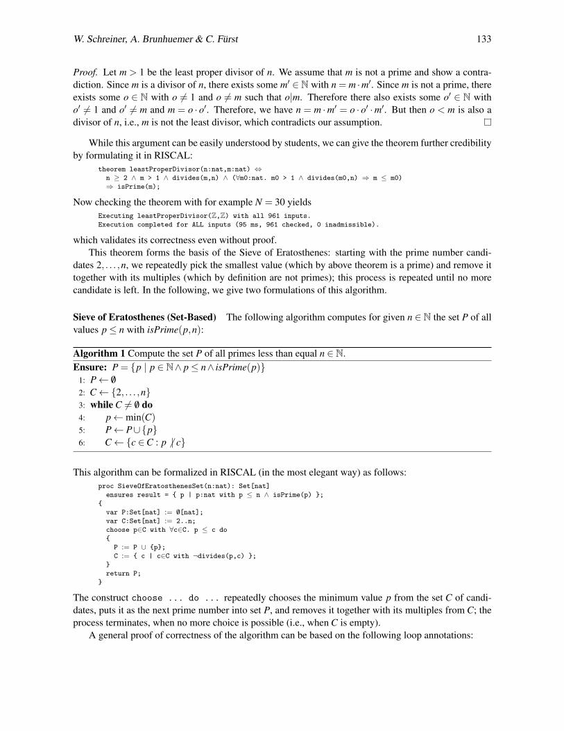
Theorem 1 (Least Proper Divisor). Let n be a natural number greater equal 2. Then the least properdivisor m > 1 of n is a prime.

W. Schreiner, A. Brunhuemer & C. Fürst 133

Proof. Let m > 1 be the least proper divisor of n. We assume that m is not a prime and show a contra-diction. Since m is a divisor of n, there exists some m′ ∈ N with n = m ·m′. Since m is not a prime, thereexists some o ∈ N with o 6= 1 and o 6= m such that o|m. Therefore there also exists some o′ ∈ N witho′ 6= 1 and o′ 6= m and m = o · o′. Therefore, we have n = m ·m′ = o · o′ ·m′. But then o < m is also adivisor of n, i.e., m is not the least divisor, which contradicts our assumption.

While this argument can be easily understood by students, we can give the theorem further credibilityby formulating it in RISCAL:

theorem leastProperDivisor(n:nat,m:nat) ⇔n ≥ 2 ∧ m > 1 ∧ divides(m,n) ∧ (∀m0:nat. m0 > 1 ∧ divides(m0,n) ⇒ m ≤ m0)⇒ isPrime(m);

Now checking the theorem with for example N = 30 yieldsExecuting leastProperDivisor(Z,Z) with all 961 inputs.Execution completed for ALL inputs (95 ms, 961 checked, 0 inadmissible).

which validates its correctness even without proof.This theorem forms the basis of the Sieve of Eratosthenes: starting with the prime number candi-

dates 2, . . . ,n, we repeatedly pick the smallest value (which by above theorem is a prime) and remove ittogether with its multiples (which by definition are not primes); this process is repeated until no morecandidate is left. In the following, we give two formulations of this algorithm.

Sieve of Eratosthenes (Set-Based) The following algorithm computes for given n ∈ N the set P of allvalues p≤ n with isPrime(p,n):

Algorithm 1 Compute the set P of all primes less than equal n ∈ N.Ensure: P = {p | p ∈ N∧ p≤ n∧ isPrime(p)}

1: P← /02: C←{2, . . . ,n}3: while C 6= /0 do4: p←min(C)5: P← P∪{p}6: C←{c ∈C : p 6 | c}

This algorithm can be formalized in RISCAL (in the most elegant way) as follows:proc SieveOfEratosthenesSet(n:nat): Set[nat]ensures result = { p | p:nat with p ≤ n ∧ isPrime(p) };

{var P:Set[nat] := /0[nat];var C:Set[nat] := 2..n;choose p∈C with ∀c∈C. p ≤ c do{

P := P ∪ {p};C := { c | c∈C with ¬divides(p,c) };

}return P;

}

The construct choose ... do ... repeatedly chooses the minimum value p from the set C of candi-dates, puts it as the next prime number into set P, and removes it together with its multiples from C; theprocess terminates, when no more choice is possible (i.e., when C is empty).

A general proof of correctness of the algorithm can be based on the following loop annotations:

134 Teaching Formalization via Automatic Checking

invariant P = { p | p:nat with p ≤ n ∧ isPrime(p) ∧ ∀c∈C. p < c };invariant C ⊆ 2..n;decreases |C|;

Here the invariants demonstrate that P contains, at every iteration of the loop, all primes that are less thanequal n and less than equal the minimum of C. Thus, when the loop terminates with C = /0, P holds allprimes less than equal n. Since the termination term |C| indicates that the size of C is decreased in everyloop iteration, this is indeed eventually the case. Checking the algorithm with N = 30

Executing SieveOfEratosthenesSet(Z) with all 31 inputs.Execution completed for ALL inputs (746 ms, 31 checked, 0 inadmissible).

validates both that the algorithm satisfies its contract and that the loop annotations are correct (if theyshould not be sufficient for a proof, they are at least not too strong).

Sieve of Eratosthenes (Array-Based) The following algorithm computes for given n ∈N the Booleanarray P of length n such that P[p] has value “true” if and only if the property isPrime(p) holds:

Algorithm 2 Compute the Boolean array P which indicates all primes less than equal n ∈ N.Ensure: ∀p ∈ N. p≤ n⇒ (P[p] = T⇔ isPrime(p))

1: P← (T,T, . . . ,T) ∈ Bn+1;2: P[0],P[1]← F;3: for p from 2 while p · p≤ n by 1 do4: if P[p] = T then5: for k from 2 while p · k ≤ n by 1 do6: P[p · k]← F

This algorithm is in essence a refinement of the set-based algorithm, where the Boolean array P takesthe role of both sets P and C: all array values at indices less than p already indicate the prime status ofthe indices while all indices greater than equal p are the candidates that remain to be processed. Theouter loop looks for the next smallest prime number p; when such a p is found, its greater multiples areremoved from the candidates. The algorithm can be formalized in RISCAL as follows:

proc SieveOfEratosthenesArray(n:nat): Array[N+1,Bool]ensures ∀p:nat with p ≤ n. result[p] ⇔ isPrime(p);

{var P:Array[N,Bool] := Array[N+1,Bool](>);P[0] := ⊥; P[1] := ⊥;for var p:nat := 2; p·p ≤ n; p := p+1 do{

if P[p] then{for var k:nat := 2; p·k ≤ N; k := k+1 do

P[p·k] := ⊥;}

}return P;

}

A verification of the algorithm can be based on the following annotations of the outer loop:invariant 2 ≤ p ∧ (p-1)·(p-1) ≤ n;invariant ∀j:nat with j < p. P[j] ⇔ isPrime(j);invariant ∀j:nat with 2 ≤ j ∧ j < p. ∀k:nat with j < k. divides(j,k) ⇒ ¬P[k];decreases n-p+2;

W. Schreiner, A. Brunhuemer & C. Fürst 135

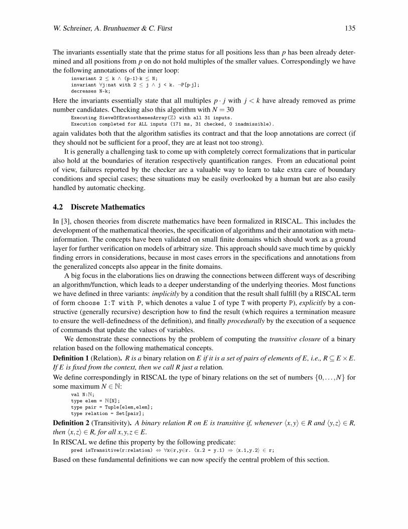
The invariants essentially state that the prime status for all positions less than p has been already deter-mined and all positions from p on do not hold multiples of the smaller values. Correspondingly we havethe following annotations of the inner loop:

invariant 2 ≤ k ∧ (p-1)·k ≤ N;invariant ∀j:nat with 2 ≤ j ∧ j < k. ¬P[p·j];decreases N-k;

Here the invariants essentially state that all multiples p · j with j < k have already removed as primenumber candidates. Checking also this algorithm with N = 30

Executing SieveOfEratosthenesArray(Z) with all 31 inputs.Execution completed for ALL inputs (171 ms, 31 checked, 0 inadmissible).

again validates both that the algorithm satisfies its contract and that the loop annotations are correct (ifthey should not be sufficient for a proof, they are at least not too strong).

It is generally a challenging task to come up with completely correct formalizations that in particularalso hold at the boundaries of iteration respectively quantification ranges. From an educational pointof view, failures reported by the checker are a valuable way to learn to take extra care of boundaryconditions and special cases; these situations may be easily overlooked by a human but are also easilyhandled by automatic checking.

4.2 Discrete Mathematics

In [3], chosen theories from discrete mathematics have been formalized in RISCAL. This includes thedevelopment of the mathematical theories, the specification of algorithms and their annotation with meta-information. The concepts have been validated on small finite domains which should work as a groundlayer for further verification on models of arbitrary size. This approach should save much time by quicklyfinding errors in considerations, because in most cases errors in the specifications and annotations fromthe generalized concepts also appear in the finite domains.

A big focus in the elaborations lies on drawing the connections between different ways of describingan algorithm/function, which leads to a deeper understanding of the underlying theories. Most functionswe have defined in three variants: implicitly by a condition that the result shall fulfill (by a RISCAL termof form choose I:T with P, which denotes a value I of type T with property P), explicitly by a con-structive (generally recursive) description how to find the result (which requires a termination measureto ensure the well-definedness of the definition), and finally procedurally by the execution of a sequenceof commands that update the values of variables.

We demonstrate these connections by the problem of computing the transitive closure of a binaryrelation based on the following mathematical concepts.Definition 1 (Relation). R is a binary relation on E if it is a set of pairs of elements of E, i.e., R⊆ E×E.If E is fixed from the context, then we call R just a relation.We define correspondingly in RISCAL the type of binary relations on the set of numbers {0, . . . ,N} forsome maximum N ∈ N:

val N:N;type elem = N[N];type pair = Tuple[elem,elem];type relation = Set[pair];

Definition 2 (Transitivity). A binary relation R on E is transitive if, whenever 〈x,y〉 ∈ R and 〈y,z〉 ∈ R,then 〈x,z〉 ∈ R, for all x,y,z ∈ E.In RISCAL we define this property by the following predicate:

pred isTransitive(r:relation) ⇔ ∀x∈r,y∈r. (x.2 = y.1) ⇒ 〈x.1,y.2〉 ∈ r;

Based on these fundamental definitions we can now specify the central problem of this section.

136 Teaching Formalization via Automatic Checking

Problem Specification and Implicit Definition Our problem is to compute the transitive closure of agiven binary relation based on the following definition.

Definition 3 (Transitive Closure). S is the transitive closure of relation R, if S is the smallest transitiverelation S that contains R, i.e., S is a subset of every transitive relation that contains R.

The corresponding RISCAL definition is:pred isTransitiveClosure(r:relation,s:relation) ⇔r ⊆ s ∧ isTransitive(s) ∧(∀s0:relation. r ⊆ s0 ∧ isTransitive(s0) ⇒ s ⊆ s0);

We claim that the transitive closure of every relation indeed exists and, furthermore, is uniquely defined:theorem transitiveClosureExists(r:relation) ⇔∃s:relation. isTransitiveClosure(r,s);

theorem transitiveClosureIsUnique(r:relation) ⇔∀s1:relation with isTransitiveClosure(r,s1).∀s2:relation with isTransitiveClosure(r,s2).

s1 = s2;

These properties can be quickly validated for N = 2:Executing transitiveClosureExists(Set[Tuple[Z,Z]]) with all 512 inputs.Execution completed for ALL inputs (675 ms, 512 checked, 0 inadmissible).Executing transitiveClosureIsUnique(Set[Tuple[Z,Z]]) with all 512 inputs.362 inputs (362 checked, 0 inadmissible, 0 ignored)...Execution completed for ALL inputs (2648 ms, 512 checked, 0 inadmissible).

Thus we can implicitly define a function which chooses a relation that satisfies the required property:fun transitiveClosureI(r:relation):relation =

choose s:relation with isTransitiveClosure(r,s);

To validate our definitions, we can execute this function for all possible inputs and inspect its results(because the result is uniquely defined, deterministic execution suffices):

Executing transitiveClosureI(Set[Tuple[Z,Z]]) with all 512 inputs.Run 0 of deterministic function transitiveClosureI({}):Result (3 ms): {}...Run 106 of deterministic function transitiveClosureI({[1,0],[0,1],[2,1],[0,2]}):Result (1 ms): {[0,0],[1,0],[2,0],[0,1],[1,1],[2,1],[0,2],[1,2],[2,2]}...Execution completed for ALL inputs (4242 ms, 512 checked, 0 inadmissible).Not all nondeterministic branches may have been considered.

Explicit (Recursive) Definition A natural approach to compute the transitive closure of a relation r asa recursive function is based on the following fundamental steps:

1. If r is transitive, then we are finished and r is our result.

2. Otherwise r contains some pairs 〈x,z〉 and 〈z,y〉 that violate the transitivity of r in the sense that〈x,y〉 is not in r. We thus add 〈x,y〉 to r and continue with step (1).

Indeed, in step (2) of the algorithm we may consider all violating pairs and add to r all the mending pairsat once. The corresponding function can be defined in RISCAL as follows:

fun transitiveClosureR(r:relation):relationensures isTransitiveClosure(r,result);decreases 2^((N+1)^2)-|r|;

= if isTransitive(r) thenr

elsetransitiveClosureR(r ∪

{ 〈x,y〉 | x:elem,y:elem with ∃p∈r,q∈r. (x = p.1 ∧ y = q.2 ∧ p.2 = q.1) });

W. Schreiner, A. Brunhuemer & C. Fürst 137

The termination of this function is guaranteed by the measure stated in the decrease clause; its correct-ness follows from the fact that the size |r| of r is increased in every recursive invocation; however, sincewe have only N +1 elements, there are at most (N +1)2 pairs in r, thus |r| can be at most 2(N+1)2

.The partial correctness of this algorithm is a direct consequence of the following theorem on which

a later verification may be based:theorem transitiveClosureCorrectness(r:relation) ⇔if isTransitive(r) then

isTransitiveClosure(r,r)else

let s = r ∪ { 〈x,y〉 | x:elem,y:elem with ∃p∈r,q∈r. (x = p.1 ∧ y = q.2 ∧ p.2 = q.1) } in∀t:relation. isTransitiveClosure(r ∪ s,t) ⇒ isTransitiveClosure(r,t);

Both the algorithm and the correctness theorem may be quickly validated for N = 2:Executing transitiveClosureR(Set[Tuple[Z,Z]]) with all 512 inputs.Execution completed for ALL inputs (699 ms, 512 checked, 0 inadmissible).Executing transitiveClosureCorrectness(Set[Tuple[Z,Z]]) with all 512 inputs.Execution completed for ALL inputs (1148 ms, 512 checked, 0 inadmissible).

Procedural Definition Another algorithm which may be easiest expressed as a procedure is based onthe following main steps:

1. We initialize the result variable res with the empty set and an auxiliary variable new with r.

2. We choose some pair x ∈ new and check for every pair y ∈ res, if the combination of x and yviolates the transitivity of res. If yes, add to new the pair that mends the violation.

3. We add x to res, remove it from new and continue with step (2).

4. When new becomes empty, the algorithm terminates and we return res as its result.

In more detail, the algorithm can be formulated in RISCAL as follows:proc transitiveClosureP(r:relation):relationensures isTransitiveClosure(r,result);

{var res:relation := /0[pair];var new:relation := r;choose x ∈ new do{for y ∈ res do{

if x.1 = y.2 ∧ ¬(〈y.1,x.2〉 ∈ res) thennew := new ∪ { 〈y.1, x.2〉 };

if x.2 = y.1 ∧ ¬(〈x.1,y.2〉 ∈ res) thennew := new ∪ { 〈x.1,y.2〉 };

}res := res ∪ { x };new := new \ { x };

}return res;

}

The termination of the algorithm can be guaranteed by adding the termination measuredecreases 2^((N+1)^2)-|res|;

to the outer loop. Similar to the recursive algorithm, its correctness follows from the fact that the size ofres is increases by every loop iteration but cannot exceed 2(N+1)2

.The partial correctness of the algorithm follows from the following invariants of the outer loop:

invariant res ∩ new = /0[pair];invariant res ∪ new ⊆ transitiveClosureI(r);invariant ∀s∈res,t∈res with s.2 = t.1. 〈s.1,t.2〉 ∈ res ∨ 〈s.1,t.2〉 ∈ new;

138 Teaching Formalization via Automatic Checking

From the second invariant, we know that in every loop iteration res is a subset of the transitive closure.Since the loop terminates when new is the empty set, the third invariant implies that then res is transitiveand thus itself the transitive closure.

The correctness of the invariant of the outer proof has to be verified with the help of the invariant ofthe inner loop:

invariant new = old_new∪ { 〈y0.1,x.2〉 | y0 ∈ forSet with x.1 = y0.2 ∧ ¬〈y0.1,x.2〉 ∈ res }∪ { 〈x.1,y0.2〉 | y0 ∈ forSet with x.2 = y0.1 ∧ ¬〈x.1,y0.2〉 ∈ res };

This invariant explicitly describes which values have been added after the termination of the loop to theoriginal value of new (special variable old_new) to get the new value.

The correctness of the algorithm with respect to its specification and the correctness of the annota-tions may be quickly validated for N = 2:

Executing transitiveClosureP(Set[Tuple[Z,Z]]) with all 512 inputs.Execution completed for ALL inputs (1217 ms, 512 checked, 0 inadmissible).Not all nondeterministic branches may have been considered.

Both loops have been expressed by non-deterministic iteration constructs choose and for which mayselect the respective elements in arbitrary order; here deterministic execution has been selected in orderto avoid the combinatorial explosion of execution branches.

With the help of the RISCAL support for parallelism, it is also possible to check larger domaininstances. For instance, we may check the instance N = 3 with 4 threads on the local computer and 16threads on a remote server in a considerable but still manageable amount of time:

Executing transitiveClosureP(Set[Tuple[Z,Z]]) with all 65536 inputs....PARALLEL execution with 4 local threads and 1 remote servers (output disabled)....Execution completed for ALL inputs (870524 ms, 65536 checked, 0 inadmissible).Not all nondeterministic branches may have been considered.

However, as emphasized before, the point of RISCAL is not so much in verifying specifications butfinding errors; typically such errors already arise in small domain instances that allow quicker checking.

5 Conclusions and Further Work

RISCAL is still in its infancy with first contents having been developed and first classroom experiencehaving been gained; subsequent experience with the use of RISCAL will shape the further developmentof language and system. This will proceed along several possible strands:

• We will automatize the generation of formulas for the validation of specifications and of verifica-tion conditions for the proof-based verification of algorithms over arbitrary size domains.

• As a (potentially more efficient) alternative to formula evaluation, we will translate formulas intoa suitable theory of the SMT-LIB library and apply SMT solvers for checking their validity.

• We will investigate the visualization of formula evaluation in order to give students quick feedbackwhy a formula is not valid.

• We will export formulas to some external prover(s) such as the RISC ProofNavigator to allow theseamless proof-based verification of formulas over arbitrary size domains.

Most important, however, we want to develop a library of specifications and accommodating lecturematerials that shall support the self-study of students in the formalization of mathematical theories andalgorithms with the ultimate goal of self-paced and self-instructed learning.

W. Schreiner, A. Brunhuemer & C. Fürst 139

References

[1] Jean-Raymond Abrial, Michael Butler, Stefan Hallerstede, Thai Son Hoang, Farhad Mehta & Laurent Voisin(2010): Rodin: An Open Toolset for Modelling and Reasoning in Event-B. International Journal on SoftwareTools for Technology Transfer 12(6), pp. 447–466, doi:10.1007/s10009-010-0145-y.

[2] Yves Bertot & Pierre Castéran (2016): Interactive Theorem Proving and Program Development — Coq’Art:The Calculus of Inductive Constructions. Springer, Berlin, Germany, doi:10.1007/978-3-662-07964-5.

[3] Alexander Brunhuemer (2017): Validating the Formalization of Theories and Algorithms of Discrete Mathe-matics by the Computer-Supported Checking of Finite Models. Bachelor thesis, Research Institute for Sym-bolic Computation (RISC), Johannes Kepler University, Linz, Austria.

[4] Bruno Buchberger, Tudor Jebelean, Temur Kutsia, Alexander Maletzky & Wolfgang Windsteiger (2016):Theorema 2.0: Computer-Assisted Natural-Style Mathematics. Journal of Formalized Reasoning 9(1), pp.149–185, doi:10.6092/issn.1972-5787/4568.

[5] Lilian Burdy, Yoonsik Cheon, David R. Cok, Michael D. Ernst, Joseph R. Kiniry, Gary T. Leavens, K. Rus-tan M. Leino & Erik Poll (2005): An Overview of JML Tools and Applications. International Journal onSoftware Tools for Technology Transfer 7(3), pp. 212–232, doi:10.1007/s10009-004-0167-4.

[6] Jon Barwise Dave Barker-Plummer, John Etchemendy & Albert Liu (2008): Tarski’s World: Revised andExpanded. CSLI Publications, Stanford, CA, USA.

[7] Jean-Christophe Filliâtre & Andrei Paskevich (2013): Why3 — Where Programs Meet Provers. InM. Felleisen & P. Gardner, editors: ESOP 2013, Rome, Italy, March 16-24, 2013, Lecture Notes in ComputerScience 7792, Springer, Berlin, Germany, pp. 125–128, doi:10.1007/978-3-642-37036-6_8.

[8] Christoph Fürst & Wolfgang Schreiner (2017): Formalization of Two Algorithms Arising in Number Theory.Technical Report, RISC, Johannes Kepler University, Linz, Austria. To appear.

[9] Daniel Jackson (2011): Software Abstractions — Logic, Language, and Analysis, revised edition. MIT Press,Cambridge, MA, USA.

[10] Leslie Lamport (2002): Specifying Systems: The TLA+ Language and Tools for Hardware and SoftwareEngineers. Addison-Wesley, Boston, MA, USA.

[11] Peter G. Larsen & John Fitzgerald (2016): The Evolution of VDM Tools from the 1990s to 2015 and the Influ-ence of CAMILA. J. Logical and Algebr. Meth. in Prog. 85(5), pp. 985–998, doi:10.1016/j.jlamp.2015.10.001.

[12] K. Rustan M. Leino (2010): Dafny: An Automatic Program Verifier for Functional Correctness. In E. M.Clarke & A. Voronkov, editors: LPAR-16, Dakar, Senegal, April 25–May 1, 2010, Revised Selected Papers,Lecture Notes in Computer Science 6355, Springer, pp. 348–370, doi:10.1007/978-3-642-17511-4_20.

[13] Tobias Nipkow & Gerwin Klein (2014): Concrete Semantics — With Isabelle/HOL. Springer, Heidelberg,Germany, doi:10.1007/978-3-319-10542-0.

[14] Tobias Nipkow, Lawrence C. Paulson & Markus Wenzel (2017): Isabelle/HOL — A Proof Assistant forHigher-Order Logic. Springer, Berlin, Germany. Available at http://isabelle.in.tum.de/doc/tutorial.pdf.

[15] RISCAL (2017): The RISC Algorithm Language (RISCAL). Available at https://www.risc.jku.at/research/formal/software/RISCAL.

[16] Daniela Ritirc (2016): Formally Modeling and Analyzing Mathematical Algorithms with Software Specifica-tion Languages & Tools. Master’s thesis, RISC, Johannes Kepler University, Linz, Austria.

[17] Wolfgang Schreiner (2009): The RISC ProofNavigator: A Proving Assistant for Program Verification in theClassroom. Formal Aspects of Computing 21(3), pp. 277–291, doi:10.1007/s00165-008-0069-4.

[18] Wolfgang Schreiner (2012): Computer-Assisted Program Reasoning Based on a Relational Semantics ofPrograms. EPTCS 79, pp. 124–142, doi:10.4204/EPTCS.79.8. ThEdu’11, Wrocław, Poland, July 31, 2011.

[19] Wolfgang Schreiner (2017): The RISC Algorithm Language (RISCAL) — Tutorial and Reference Manual(Version 1.0). Technical Report, RISC, Johannes Kepler University, Linz, Austria. Download from [15].