Team Green

Team GreenTeam GreenJohn BarkerJohn BarkerJohn BeverlyJohn BeverlyKeith SkilesKeith Skiles

UTC ENGR329-001UTC ENGR329-0012-15-062-15-06

Steady State and Step Response Steady State and Step Response PerformancePerformance

Speed Control SystemSpeed Control System

OutlineOutline

System BackgroundSystem Background– Description, SSOC, Step ResponseDescription, SSOC, Step Response

FOPDT ModelFOPDT Model Model TheoryModel Theory ResultsResults ConclusionsConclusions

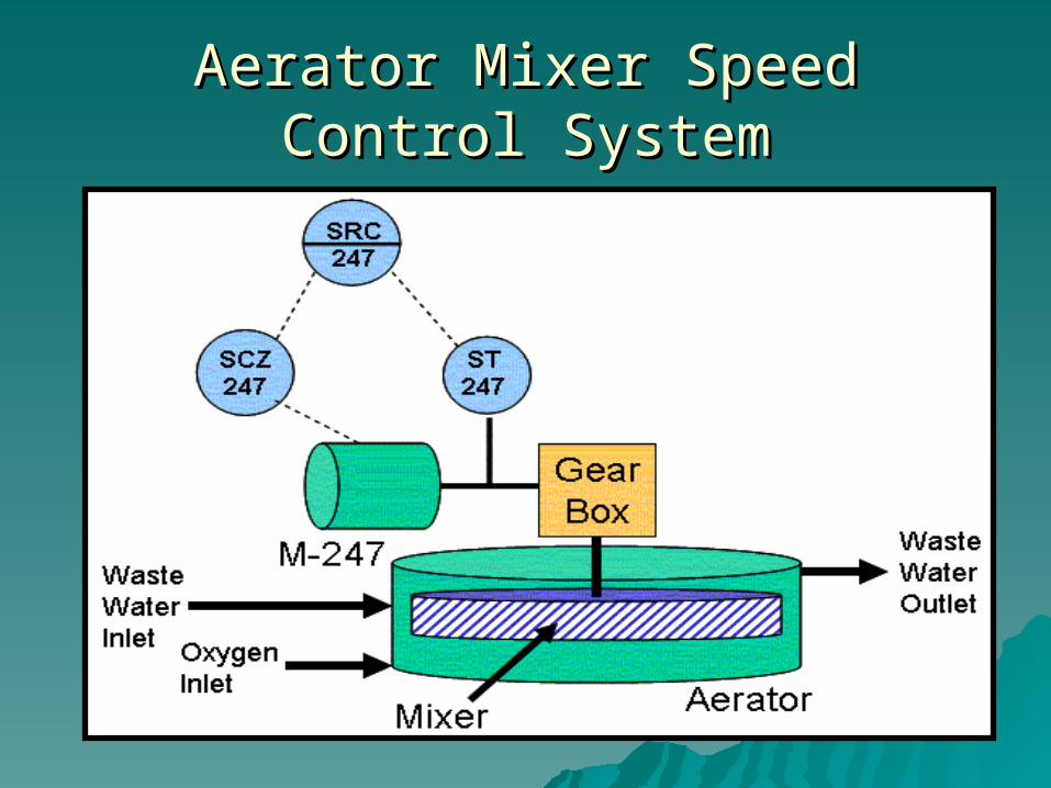
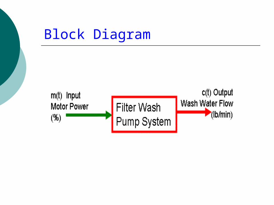
Aerator Mixer Speed Control Aerator Mixer Speed Control SystemSystem

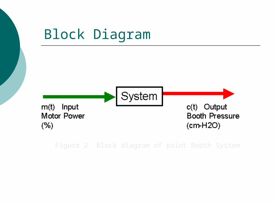
Block Diagram of SystemBlock Diagram of System

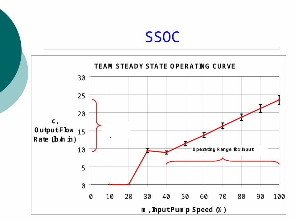
Steady State Operating Curve

0

200

400

600

800

1000

1200

1400

1600

1800

0 20 40 60 80 100

Motor Input (%)

Sp

eed

Ou

tpu

t (R

PM

)

Slope = 17.4

Sample Step Response Curve

0

100

200

300

400

500

600

700

800

0 2 4 6 8 10

Time (s)

Ou

tpu

t (R

PM

)


0

200

400

600

800

1000

1200

1400

1600

1800

0 20 40 60 80 100

Motor Input (%)

Sp

eed

Ou

tpu

t (R

PM

)

Low

High

Mid

Time Response (Gain)Time Response (Gain)

Gain

17

17.1

17.2

17.3

17.4

17.5

Low Up Mid Up High Up Low Down Mid Down High Down

System Gain (RPM/%)

Time Response (Dead Time)Time Response (Dead Time)Dead Time (s)

0.08

0.09

0.1

0.11

0.12


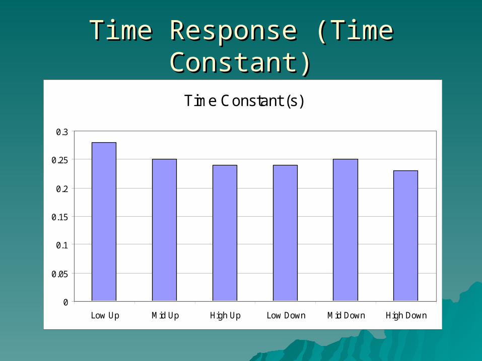
Time Response (Time Constant)Time Response (Time Constant)

Time Constant (s)

0

0.05

0.1

0.15

0.2

0.25

0.3


Step Response Values and ErrorsStep Response Values and Errors

K (RPM/%) t0 (s) τ (s)

Average 17.4 0.11 0.25

Std. Dev 0.05 0.006 0.017

Laplace Domain FOPDT ModelLaplace Domain FOPDT Model

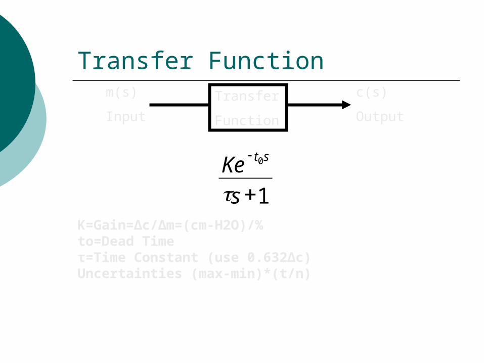
System Transfer FunctionSystem Transfer Function G(s) = G(s) = Ke /Ke /ττs+1s+1

– ParametersParameters

tt00=Dead Time=Dead Time

K = System GainK = System Gain

ττ = Time Constant = Time Constant

-t0s

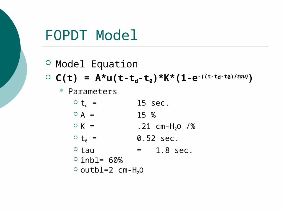
FOPDT ModelFOPDT Model

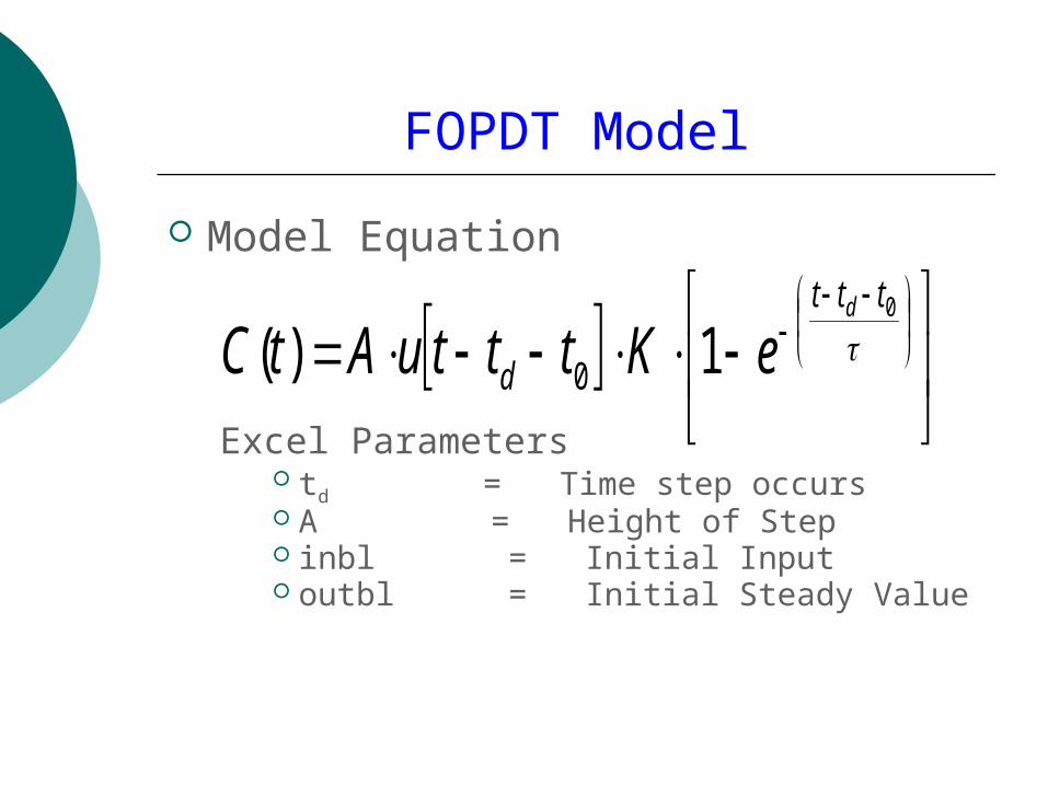
Model Equation in Time DomainModel Equation in Time Domain– C(t) = A*u(t-tC(t) = A*u(t-tdd-t-t00)*K*(1-e ))*K*(1-e )-(t-td-t0)

0

100

200

300

400

500

600

700

800

0 2 4 6 8 10

Time (s)

Ou

tpu

t (R

PM

)

0

6

12

18

24

30

36

42

48

Inp

ut

(%)

Model Output

Real Output

Model Input

Real Input

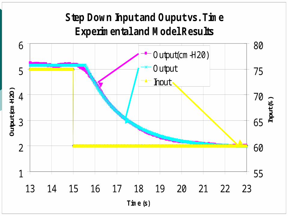
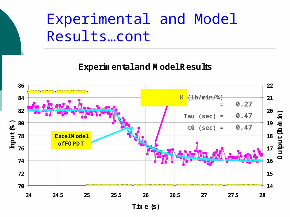
ResultsResults

0

100

200

300

400

500

600

700

800

4.5 5 5.5 6 6.5

Time (s)

Ou

tpu

t (R

PM

)

0

6

12

18

24

30

36

42

48

Inp

ut

(%)

Model Output

Real Output

Model Input

Real Input

Time Response (Gain)Time Response (Gain)

Gain (RPM/%)

02468

101214161820

Low Mid High

Time Response (Dead Time)Time Response (Dead Time)

Dead Time (s)

0

0.02

0.04

0.06

0.08

0.1

0.12

Low Mid High

Time Response (Time Constant)Time Response (Time Constant)

Time Constant (s)

0

0.05

0.1

0.15

0.2

0.25

Low Mid High

Overall ResultsOverall ResultsExperimental Results:Experimental Results:

Steady State Gain : K= 17.1RPM/% ± 0.10Steady State Gain : K= 17.1RPM/% ± 0.10

Dead Time : tDead Time : t00= 0.06s ± 0.012= 0.06s ± 0.012

Time Constant : Time Constant : τ τ = 0.19s ± 0.034= 0.19s ± 0.034

Model Results:Model Results:

Steady State Gain : K= 17.4RPM/%Steady State Gain : K= 17.4RPM/%

Dead Time : tDead Time : t00= 0.1s= 0.1s

Time Constant : Time Constant : τ τ = 0.23s= 0.23s

ConclusionsConclusions

Operating Range 150-1700RPMOperating Range 150-1700RPM K = 17.4 RPM/%K = 17.4 RPM/% tt00= 0.1s= 0.1s ττ = 0.23s= 0.23s

Red Team -Pressure-Steady State Operating And Step Response

Dennis ToCory RichardsonJamison Linden

04/21/23, UTC, ENGR-329

Contents

Background Description, SSOC, Step Response

FOPDT Model Model Theory Results Conclusions

Background

System Input Output SSOC Operating Range

System

Figure 1. Schematic diagram of the Dunlap Plant Spray-Paint Booths

Block Diagram

Figure 2. Block diagram of paint Booth System

SSOC


0

2

4

6

8

10

12

0 10 20 30 40 50 60 70 80 90 100

m, Input Blower Pressure (%)

c, Output Pressure (cm-H20)

Operating Range for Output

Operating Range for Input

Operating Range

Input operating range (45%-90%)

Output operating range (0.5-10 cm-H2O)

Theory

Transfer Function Parameters

Transfer FunctionTransfer

Function

m(s)

Input

c(s)

Output

1

0

s

Ke st

K=Gain=∆c/∆m=(cm-H2O)/%to=Dead Timeτ=Time Constant (use 0.632∆c)Uncertainties (max-min)*(t/n)

Parameters


0

2

4

6

8

10

12

0 10 20 30 40 50 60 70 80 90 100

m, Input Blower Pressure (%)

c, Output Pressure (cm-H20)

Lower Upper

Middle

Results

Experimental (Step-up, Step-down) Time Response (Gain) Time Response (Dead Time) Time Response (Time Constant)

Experimental (Step-up)

Step Response Inputs and Outputs

80

82

84

86

88

90

92

13 15 17 19 21 23

Time (sec)

Inp

ut

m(t

) (%

)

0

2

4

6

8

10

12

Ou

tpu

t c

(t)

(cm

-H2

O)

Input Value(%)

Output(cm-H20)

Experimental (Step-down)

Step Response Inputs and Outputs

74767880828486889092

13 15 17 19 21 23

Time (sec)

Inp

ut

m(t

) (%

)

0

2

4

6

8

10

12

Ou

tpu

t c

(t)

(cm

-H2

O)

Input Value(%)

Output(cm-H20)

Time Response (Gain)

Step Response

0.00

0.10

0.20

0.30

0.40

0.50

0.60

0.70

Lower-up

Lower-down

Mid-up

Mid-down

Upper-up

Upper-down

Gain (cm-H2O/%)

`

Time Response (Dead Time)

Step Response

0.0

0.1

0.2

0.3

0.4

0.5

0.6

Lower-up

Lower-down

Mid-up

Mid-down

Upper-up

Upper-down

Dead Time (sec)

Time Response (Time Constant)

Step Response

0.0

0.2

0.4

0.6

0.8

1.0

1.2

1.4

1.6

1.8

2.0Tau (sec)

Lower-up

Lower-down

MId-up Mid-down

Upper-up

Upper-down

FOPDT Model

Model Equation C(t) = A*u(t-td-t0)*K*(1-e-((t-td-t0)/tau))

Parameters td = 15 sec. A = 15 % K = .21 cm-H2O /% t0 = 0.52 sec. tau = 1.8 sec. inbl= 60% outbl=2 cm-H2O

Step Up Input and Ouput vs. TimeExperimental and Model Results

1

2

3

4

5

6

13 14 15 16 17 18 19 20 21 22 23

Time (s)

Out

put (

cm-H

2O)

55

60

65

70

75

80

Inpu

t (%

)

Output(cm-H20)

Output

Input

Step Down Input and Ouput vs. TimeExperimental and Model Results

1

2

3

4

5

6

13 14 15 16 17 18 19 20 21 22 23Time (s)

Out

put (

cm-H

2O)

55

60

65

70

75

80

Inpu

t (%

)

Output(cm-H20)

Output

Input

Model Time Response (Gain)

Model Time Response (Gain)

0.0

0.1

0.2

0.3

0.4

Gain (cm-H2O)

Lower Up

Lower Down

Middle Up

MiddleDown

Upper Up

UpperDown

Model Time Response (Dead Time)

Step Response

0.0

0.1

0.2

0.3

0.4

0.5

0.6

Lower-up

Lower-down

Mid-up Mid-down

Upper-up Upper-down

Dead Time (min)

Model Time Response (Time Constant)Step Response

0.0

0.2

0.4

0.6

0.8

1.0

1.2

1.4

1.6

1.8

2.0Tau (min)

Lower-up

Lower-down

MId-up Mid-up Upper-up

Upper-up

Results

EXPERIMENTAL PARAMETERS INCREASING

STEADY STATE GAIN K 0.1-0.35 cm-H2O/% DEAD TIME to 0.5 s

TIME CONSTANT t 1.7 s

EXPERIMENTAL PARAMETERS DECREASING

STEADY STATE GAIN K 0.1-0.35 cm-H2O /% DEAD TIME to 0.5 s TIME CONSTANT t 1.7 s

Conclusions

Input operating range Output operating range (K) goes up as the input % is

increased (0.1-0.35cm-H2O/%) (to) stays constant (0.5sec) ( ) stays constant (1.7sec)

Flow Rate Control System

“Step Response Modeling”

February 15, 2006U.T.C.

Engineering 329

Yellow Team

Jimy George Jeff LawrenceTaylor Murphy Jennifer Potter

Outline

System Background Description, SSOC, Step Response

FOPDT Theory Model Theory Results Conclusions

Flow System Setup

Block Diagram

Steady State Operation

Flow Rate Versus Time @ 80% Input

7576777879808182838485

0 10 20 30 40

Time (s)

Po

wer

Inp

ut

(%)

0

5

10

15

20

25

Flo

w R

ate

(lb

/min

)

Input

Output

Steady Operation

SSOC

TEAM STEADY STATE OPERATING CURVE

0

5

10

15

20

25

30

0 10 20 30 40 50 60 70 80 90 100

m, Input Pump Speed (%)

c, Output Flow Rate (lb/min)

Operating Range for Input

Operating Range for Output

Step Response: 70%-85%

FOPDT Model

Transfer Function

1

0

s

Ke st

FOPDT Model

Model Equation

Excel Parameters td = Time step occurs A = Height of Step inbl = Initial Input outbl = Initial Steady Value

0

1)( 0

ttt

d

d

eKtttuAtC

Experimental and Model Results


70

72

74

76

78

80

82

84

86

24 24.5 25 25.5 26 26.5 27 27.5 28

Time (s)

Inp

ut

(%)

14

15

16

17

18

19

20

21

22

Ou

tpu

t (l

b/m

in)

Excel Model of FOPDT

Experimental Values

K (lb/min/%) = 0.26

Tau (sec) = 0.46

t0 (sec) = 0.42

Experimental and Model Results…cont


70

72

74

76

78

80

82

84

86

24 24.5 25 25.5 26 26.5 27 27.5 28

Time (s)

Inp

ut

(%)

14

15

16

17

18

19

20

21

22

Ou

tpu

t (l

b/m

in)

Excel Model of FOPDT

Experimental Data K (lb/min/%) = 0.27

Tau (sec) = 0.47

t0 (sec) = 0.47

Results

Week 3 Values of K

Step down

Step Up Step Up

Step Down

Step UpStep Down

Step Up

Step Down

0

0.05

0.1

0.15

0.2

0.25

0.3

1 2 3 4 5 6 7 8

Trial

K (lb

/min

/%)

45%-55% 55%-70% 70%-85% 85%-100%

Week 3 Values of K

Step down

Step Up Step Up

Step Down

Step UpStep Down

Step Up

Step Down

0

0.05

0.1

0.15

0.2

0.25

0.3

1 2 3 4 5 6 7 8

Trial

K (lb

/min

/%)

45%-55% 55%-70% 70%-85% 85%-100%

Week 6 Values of K

Step down

Step Up Step Up

Step Down

Step Up

Step Down

Step Up

Step Down

0

0.05

0.1

0.15

0.2

0.25

0.3

1 2 3 4 5 6 7 8

Trial

K (lb

/min/

%)

45%-55% 55%-70% 70%-85% 85%-100%

Week 6 Values of K

Step down

Step Up Step Up

Step Down

Step Up

Step Down

Step Up

Step Down

0

0.05

0.1

0.15

0.2

0.25

0.3

1 2 3 4 5 6 7 8

Trial

K (lb

/min/

%)

45%-55% 55%-70% 70%-85% 85%-100%

Results … cont

Week 3 Values of Tau

Step down

Step Up Step Up

Step Down

Step Up

Step Down

Step Up

Step Down0

0.1

0.2

0.3

0.4

0.5

0.6

0.7

1 2 3 4 5 6 7 8

Trial

Tau

(sec)

45%-55% 55%-70% 70%-85% 85%-100%


Step down

Step Up Step Up

Step Down

Step Up

Step Down

Step Up

Step Down0

0.1

0.2

0.3

0.4

0.5

0.6

0.7

1 2 3 4 5 6 7 8

Trial

Tau

(sec)

45%-55% 55%-70% 70%-85% 85%-100%


Step down

Step Up Step Up

Step Down

Step Up

Step Down

Step Up

Step Down0

0.1

0.2

0.3

0.4

0.5

0.6

0.7

1 2 3 4 5 6 7 8

Trial

Tau (

sec)

45%-55% 55%-70% 70%-85% 85%-100%


Step down

Step Up Step Up

Step Down

Step Up

Step Down

Step Up

Step Down0

0.1

0.2

0.3

0.4

0.5

0.6

0.7

1 2 3 4 5 6 7 8

Trial

Tau (

sec)

45%-55% 55%-70% 70%-85% 85%-100%


Step down

Step Up Step Up

Step Down

Step Up

Step Down

Step Up

Step Down0

0.1

0.2

0.3

0.4

0.5

0.6

0.7

1 2 3 4 5 6 7 8

Trial

Tau (

sec)

45%-55% 55%-70% 70%-85% 85%-100%

Results… cont

Week 3 Values of t0

Step down

Step Up Step Up

Step Down

Step Up

Step Down

Step Up

Step Down0

0.1

0.2

0.3

0.4

0.5

0.6

1 2 3 4 5 6 7 8

Trial

t 0 (s

ec)

45%-55% 55%-70% 70%-85% 85%-100%

Week 3 Values of t0

Step down

Step Up Step Up

Step Down

Step Up

Step Down

Step Up

Step Down0

0.1

0.2

0.3

0.4

0.5

0.6

1 2 3 4 5 6 7 8

Trial

t 0 (s

ec)

45%-55% 55%-70% 70%-85% 85%-100%

Week 6 Values of t0

Step down

Step Up Step Up

Step Down

Step Up

Step Down

Step Up

Step Down

0

0.1

0.2

0.3

0.4

0.5

0.6

1 2 3 4 5 6 7 8

Trial

t 0 (s

ec)

45%-55% 55%-70% 70%-85% 85%-100%

Week 6 Values of t0

Step down

Step Up Step Up

Step Down

Step Up

Step Down

Step Up

Step Down

0

0.1

0.2

0.3

0.4

0.5

0.6

1 2 3 4 5 6 7 8

Trial

t 0 (s

ec)

45%-55% 55%-70% 70%-85% 85%-100%

Week 6 Values of t0

Step down

Step Up Step Up

Step Down

Step Up

Step Down

Step Up

Step Down

0

0.1

0.2

0.3

0.4

0.5

0.6

1 2 3 4 5 6 7 8

Trial

t 0 (s

ec)

45%-55% 55%-70% 70%-85% 85%-100%

MODEL PARAMETERSDECREASING

STEADY STATE GAIN K 2.5 V/%

DEAD TIME to 0 s

TIME CONSTANT 0.6 s / 1.2 s / 2.4 s

EXPERIMENTAL PARAMETERSDECREASING

STEADY STATE GAIN K 2.5 V/%

DEAD TIME to 0 s

TIME CONSTANT 0.2 s

OVERALL RESULTS

MODEL PARAMETERS

STEADY STATE GAIN,K = 0.25 lb/min/%

DEAD TIME, to = 0.45 s

TIME CONSTANT, 0.48 s

EXPERIMENTAL PARAMETERS

STEADY STATE GAIN,K = 0.25 lb/min/%

DEAD TIME, to = 0.39 s

TIME CONSTANT, 0.51 s

OVERALL RESULTS

bOVERALL RESULTS

Experimental ErrorStandard Deviations

STEADY STATE GAIN,K = ± 0.01(lb/min/%)

DEAD TIME, to = ± 0.08 (sec)

TIME CONSTANT, ± 0.03 (sec)MODEL ErrorStandard Deviation

STEADY STATE GAIN,K = ± 0.01 (lb/min/%)

DEAD TIME, to = ± 0.02 (sec)

TIME CONSTANT, ± 0.04 (sec)

Date post:	09-Jan-2016
Category:	Documents
Upload:	chesna
View:	99 times
Download:	7 times

Team Green

Documents