Technical Analysis and Nonlinear Dynamics Vasco Jorge Salazar Soares* Abstract In this paper we develop one simple nonlinear model of time series generation that can reproduce some technical behaviours like Elliot Waves and lateral trends. Our model can forecast some technical movements as a consequence of “motion driver” at some time moments. Changing the “amplitude” of emotion stated in the “motion driver” parameter can alter technical figures. Our model is important because, to our knowledge, is the first model that can explain why there are Elliot Waves with Fibonacci ratios precisely. However, future research and development is needed since our model is only the first step. Introdution This days technical analysis is gaining substantial importance in the work of financial analysts and professionals, even theoretical explanation of the technical analysis techniques remains to be done. It is usually recognized that technical analysis is more one art than one science, regarding the efficient market theory statement that excludes technical analysis from having prediction value. However, theoretical explanation is needed always to validate some tools used since, as technical analysis state, some kinds of behaviour like Elliot movements are indeed observed in financial markets. The principal goal of our work is indeed explaining why Elliot waves work in practice and why fibonacci numbers 0,618 and 1,618 may work for expansion and retracement movements. Our past work with nonlinear and chaotic movements research leaves us with some tools to try to explain Elliot waves. For doing so, in this paper we explain very quicky chaotic theory and fractal properties of nonlinear logistic equation reproducing feigenbaums work. Our present work shows theoretically and mathematically how logistic equation can generate wave movements in precisely fibonnacci statemnents. In first part we describe the basics of technical analysis and in part two we devellope chaotic nonlinear theory with the help of logistic equation work of feigenbaum. In part three we link the two kind of analysis showing that some technical movements are simplest consequence of nonlinear dynamics, namely Elliot waves with fibonacci expansions and retracements. For completing our theoretical link between chaotic nonlinear theory and fractal movements and technical analysis, we give some practical examples in part IV. Finally we made some conclusions.
Transcript
Technical Analysis and Nonlinear Dynamics Vasco Jorge Salazar Soares*
Abstract
In this paper we develop one simple nonlinear model of time series generation that can reproduce some technical behaviours like Elliot Waves and lateral trends. Our model can forecast some technical movements as a consequence of “motion driver” at some time moments. Changing the “amplitude” of emotion stated in the “motion driver” parameter can alter technical figures. Our model is important because, to our knowledge, is the first model that can explain why there are Elliot Waves with Fibonacci ratios precisely. However, future research and development is needed since our model is only the first step.
Introdution
This days technical analysis is gaining substantial importance in the work of financial analysts and professionals, even theoretical explanation of the technical analysis techniques remains to be done. It is usually recognized that technical analysis is more one art than one science, regarding the efficient market theory statement that excludes technical analysis from having prediction value. However, theoretical explanation is needed always to validate some tools used since, as technical analysis state, some kinds of behaviour like Elliot movements are indeed observed in financial markets. The principal goal of our work is indeed explaining why Elliot waves work in practice and why fibonacci numbers 0,618 and 1,618 may work for expansion and retracement movements. Our past work with nonlinear and chaotic movements research leaves us with some tools to try to explain Elliot waves. For doing so, in this paper we explain very quicky chaotic theory and fractal properties of nonlinear logistic equation reproducing feigenbaums work. Our present work shows theoretically and mathematically how logistic equation can generate wave movements in precisely fibonnacci statemnents. In first part we describe the basics of technical analysis and in part two we devellope chaotic nonlinear theory with the help of logistic equation work of feigenbaum. In part three we link the two kind of analysis showing that some technical movements are simplest consequence of nonlinear dynamics, namely Elliot waves with fibonacci expansions and retracements. For completing our theoretical link between chaotic nonlinear theory and fractal movements and technical analysis, we give some practical examples in part IV. Finally we made some conclusions.
1.Technical Analysis, Market analysis and Statistical Evidence. 1.1.Technical Analysis concept – Information discount and Dow Theory.
1.1.1. Introdution. Since long time ago, predicting stock market movements has been one goal of market participants, some of them, looking for the holly grail. It is not surprising, understanding this whisper, that a lot of people find interesting to apply several disciplines and trying to make believe investors that the method applied is infallible in predicting stock market movements, so that investors who follow this will be rich. As we know, many of these people win money selling books instead of making money with the techniques they refer as profitable. As a matter of fact, after so many time there are 3 schools that remain active and have followers in the stock market. This schools are:
- Technical Analysis. - Fundamental Analysis. - Quantitative Analysis.
The older schools are technical analysis and fundamental analysis. Even today they are be more followed by stock market analysts and investors. The two schools base their analysis in the concept that information is not fully reflected in the stock prices. The concept that the market is efficient, latter designed by Fama(1970) , said that all information is reflected in stock prices and new information is immediately reflected in the price. Technical and Fundamental analysis did not agree with this idea and they try to understand how information released could affect future price movements of stock prices. Fundamental analysis is concerned with the value of the stock. This value is analysed comparing the cash flow statements in the past with perspectives in the future. The value of one company is determined by the discounted cash-flow that the company will generate in the future. Knowing this value, the fundamental investor only compares it with stock price and, if the price is below value the decision is buy and hold the stock. The fundamental investor believes that somewhere in the future the price will flutuate under and below fundamental value trend. So, somewhere in the future the investor that buys the stock bellow value will have opportunity to sell the stock with profit. Technical analysis is a technique that tries to extrapolate trends and stock market behaviours from past performances of prices and volumes. For the technical analyst stock market can be forecasted and that is why he studies the graphics of stock market prices and volumes. For him, what accounts is only price/volume since value is always
a subjective think that market players try to establish everyday. Technical analyst believes that information that comes to market is not immediately reflected in stock prices since not everybody know it. For the technical analyst market discounts everything and everything is reflected in the forces of demand and supply. As any economist knows, in the market there is a fight between demand and supply and the result is quantity and price at one equilibrium level. So, for the technical analyst, the two vectors that matters are price and volume of negotiation. If there is some strong volume force, and price tends to decline this means that supply is increasing slowly (not immediately since information is not immediately reflected in price) and the price will go down in the future in one movement that technical analysts call distribution movement. If there is some strong volume force and price tends to go up this means that demand is increasing slowly (not immediately since information is not immediately reflected in price) and the price will go up in the future in one movement that technical analysts call accumulation movement. Quantitative analysts, by their side,believe that the stock market is efficient, that is, the information released is immediately reflected in stock prices. So, trying to forecast or find stocks below value is a useless pratic as is looking for graphs or historical stock prices and volumes. The better way of acting in stock market is diversify and reduce intrinsic risk from stocks, concentrating in market risk. The portfolio that investor build must be aggressive or defensive against market behaviour, and this depends on risk and market expectations of the investor. For the quantitative analysts all that accounts is the risk of the portfolio against the market and eventually other factors that account for systematic risk (Ross (1976), Fama and French (1993)). Next we will see with more detail the concept of technical analysis that Dow left us. 1.1.2. Dow Theory. 1.1.2.1. Dow Theory History. The Dow Theory evolved from the work of Charles H. Dow, from a serie of articles published in the Wall Street Journal Editorials between 1900 and 1902. Dow used the behaviour of the stock market as a barometer of business conditions. His successor, William Peter Hamilton developed Dow´s principles and organized them in the Dow Theory. As a matter of fact it was a cortesy call Dow Theory since it is more Hamilton theory. These principles were latter published in 1922 in his book “The Stock Market Barometer”. This work has been accomplished with the contribute of Robert Rhea that published Dow Theory in 1932.
The teory assumes that the majority of the stocks follow market trends most of the time and that market trends exist and can be measured. In order to measure the market, Dow constructed two indexes: - The Dow Jones Industrial Average that includes 12 companies (now has 30). - The Dow Jones Rail Average that includes 12 railroad stocks. Since the Rail Average was intended for measuring transportation stocks, the historical evolution of aviation and others forms of transportation has as consequence the modification of the Rail Average. Consequently, this index has been renamed as Transportation Average. 1.1.2.2. Dow Theory Interpretation. As a first task we have to record daily closing prices of the two averages and the total os transactions in the New York Stock Exchange. The six basic assumptions of the theory are as follows: Averages Discount Everything Changes in the daily closing prices reflect the aggregate judgement and emotions of all the stock market participants. It is therefore logic to assume that the stock market discounts everything known that can affect demand and supply of stocks. The Market has Three Movements There are simultaneously three movements in the stock market. Primary Movement. The most important movement of stock markets is the primary or major trend, that is known as a bull (rising) or bear (falling) market. Such movements last for one to several years, A primary bear market is a long decline interrupted by some rallies (secondary reactions). It begins as there is some disappointment about stock behaviour in the market. The second phase reaches as the levels of business activity and profits decline. The third phase is related to liquidation of stocks regardless their value and represents the possible bottom of the bear market. A primary bull market is a long upward movement perturbed by some rallies (secondary reactions). The bull begins when the averages have discounted the worst possible news and confidence about the future begins to revive. The second phase begins when profits outperform expectations and business conditions improve. The third and final phase of the bull markets arrives when expectations are too high and the made projections are unfounded. Secondary Reactions. A secondary or intermediate reaction is defined as a important decline in a bull market or a advance in a bear market. This movements usually last from 3 weeks to some months. The movement generally retraces, as Pring (1991,pp.34)
refers, from 33 to 66 percent and sometimes it retraces 50 percent. As we will see later, the retracement percentage is a normal implication of nonlinear dynamic systems. Minor Movements. The minor movements lasts from a matter of hours up to as long as 3 weeks. It is important because it forms part of the primary or secondary moves, so it has no forecasting power for long-term investors. This is important since short-term movements can be manipulated to some degree, unlike the secondary or primary trends. Lines Indicate Movement Rhea (1932) defined a line as “ a price movement two to three weeks or longer, during which period the price variation of both averages moves within a range of approximately 5 percent (of their mean average). Such a movement indicates either accumulation (bullish movement) or distribution (bearish movement). An advance above the limits of the “line” indicates accumulation and predicts higher prices, and vice versa. Price/Volume Relationships Provide Background The normal relationship is for volume to expand on rallies and contract on declines. If volume becomes dull on a price advance and expands on a decline, a warning is giving that the prevailing trend may soon be reversed. This principle should be used as a background information, since reversals must be confirmed only by the price of the respective averages. Price Action Determines the Trend Bullish indications are given when successive rallies penetrate peaks. If price movement takes the averages below last correction in a bull market, we may believe market trend is in a way of being changed. Technical analysts prefer to use more indicators to confirm. The peaks are known as resistance levels since they are relative maximums that past market behaviour was inable to defeat. So they act as critical levels for evaluating market behaviour in the future. If price rise and beats previous peaks we are in the presence of a strong bull market. In a bull market there are some corrections that lead to minimum levels known as bottoms or support levels, since they are the levels of prices that in the past the market movement support the down movement. The Averages Must Confirm It is always assumed that a trend exist until a reversal is proved. It is normal that when we assist to one economic rebound, side by side with economic output expansion that must be transportation activity increase of these products. Of course these, in 1900´s the transportation need was more important than today, since the economy in 2000´s is more concentrated on services and transportation, even is needed it is not in the same intensity as before.
So, it is perfectly natural that today technical analysts did not had these necessity of the confirmation of averages. 1.2.Rational Investor and Psycologic Behavior. The work of Von Neuman and Morgenstern (1953) give to the economists the tool of rational investor, that is, one investor that is perfectly rational in all conditions and collective. Rational investors always look for risk when he can have better returns. Risk/return relationship is the building stone of modern portfolio theory and some of the builders, like Markowitz(1952), Sharpe(1964), Lintner(1965) and Mossin(1966) have win some nobel premiums in the 90´s. However, some psychologists like Tversky and Kahneman(1979) have shown that human behaviour may be very far from rational situations and emotion can take place in the mind of investors when they are placed in some collective circunstances. Fads, bubbles and even technical analysis techniques start to be tested hard in the latter 90´s, after the work of Scheinkman and Lebaron(1989). In that study, they have shown that some technical analysis techniques, like moving averages of 50 and 200 days can give signals with returns higher than that of risk /return relationships would predict. Fads, bubbles and stock crashes had been in the open eyes of investors and academics, where some look for rational explanations, desmistifying irrational behaviour,and others trying to shown that these kind of behaviours is the result of non rational behaviour. Shiller(1989), for example, has documented excess volatility in stock prices regarding the forecastable volatility in stock dividends in the American stock market. Exuberance irrationality is perhaps one important way for explaining stock market behaviours and is fads, bubbles and stock market crashes that happen sometimes. Resistance and support levels explained below are examples of psychological behaviour that can emerge in one collective group interation. Barberis e al.. (1998) propose a model of investor sentiment where we see prospect theory with irrational behavioural. 1.3.Price Patterns , Resistance, Support Levels and Psychological View. Technical analysts give a lot of importance to resitant and support levels. To one technical analyst market discounts everything and every day is one fight between buyers and sellers. One appreciation in price must be one consequence of volume since pressure on demand is present. If that is not the case, price appreciation could be market manipulation. One depreciation of market price must be consequence of volume since offer pressure is present. As in the demand case, if this is not the case, price depreciation could be market manipulation.
In this environment, if some high relative price is hit and market price drops after that, this price is difficult to be passed. This higher price is known as a resistance, since it is possible that offers will be heavy placed in this price. In the same thinking scheme, if some lower relative price is hit and market price appreciate after that, this price is difficult to be passed down. This lower price is known as a support, since it is possible that buyers will be heavy placed at this price. As we mention before, technical traders are always trying to predict future movements and to establish figures that may have some forecasting value in the future price movements. In this work it is not our ambition to explain some technical figures like head-and-shoulders or diamonds. Our concentration here is focused in Elliot wave explanation. 1.4.Trends, Moving Averages and Statistical Tests for Profitable Trend Strategies. As we mention before, technical analysts believe market follows trends. Primary, secondary and terciary trends, that represent different time spans are present in the stock market. If we believe that markets reflects economy, since economy follows cycles, markets must follow cycles as well. Technical analysis tries hard to measure cycles and change of the primary trends included. There are two ways of measuring trend behaviour: Trend Lines and Moving Averages. We will review very quickly this concepts. 1.4.1.Trend Lines Trend lines may define the primary, secondary and terciary movements. The trend lines are build joining support (in one uptrend line) or resistant (in one downtrend) levels between some time lags. If we joint support and resistant levels simultaneously we get chanel trends that are figures for identifying peak or bottom levels. In trend design we must know that for getting primary trends, we must get annual supports or resistant levels before we join points. In the secondary reaction as well, we may find neighbour resistant and support levels in periods away at least one month and no more than one year. This is one important consequence of primary and secondary trend definitions. For the technical analyst, if some trend line is broken, he believes that another movement will follow and he must change his attitude in the market. 1.4.2. Moving Averages.
Moving averages are popular technical analysis indicators of trend movement. Rising moving averages indicates market strength and a decline denotes weakness. Since moving averages indicate trend some popular moving averages are used to try to specify Dow Theory. 50 day moving average are used to express secondary trend and 200 day moving average are used to get primary trend. Technical analysts usually observe the ascending and descending cross of 200 moving average by the 50 day moving average to express buy and sell signs, since they believe this crossings express one change in the course of primary trend. Ascending 50 day moving averages indicates secondary trend positive. If primary trend is ascending and this 200 moving average has one value less than the 50 moving average, we are technically speaking in one Bull Market. If primary trend is descending and this 200 moving average has one value bigger than the 50 moving average, we are technically speaking in one Bear Market. Brock e al (1992) show in one important study that the 50-200 moving average strategy applied to Dow Jones Industrial Average between 1897 and 1986 produced significant signs, since sell signals are correlated with negative returns and buy signals with positive returns. Sell signals are linked to high volatility and buy signals with low volatility. Using several statistical models like ARMA and GARCH models, this autors specify the anomalous forecasting ability of this technical strategy compared with the models that cannot explain this fact. Brock e al (1992) refer explicitly (pp.1759). “ This paper shows that the return-generating process of stocks is probably more complicated than suggested by the previous studies using linear models. It is quite possible that technical rules pick up soe of the hidden patterns. We would like to emphasize that our analysis focuses on the simplest trading rules. Other more elaborate rules may generate even larger differences between conditional returns. Why suck rules might work is an intriguing issue left for further studies”. 1.5.Elliot Waves and Fibonacci Series. 1.5.1. History of Elliot Waves. Elliot Wave Principle came out in November 1978 by Robert Prechter. This theory begun many years before, when he met Elliot through correspondence. Prechter was publishing a national weekly stock market belletin to wich Elliot wished to join efforts. Letters back and forth followed but the matter was triggered in the first quarter of 1935. On that occasion the stock market, after receding from a 1933 high to a 1934 low, had started up again but during 1935´s first quarter the Dow Railroad Average broke to under its 1934 low point. Investors, economists, and stock market analysts had not recovered from the 1929-32 unpleasentness and this early 1935 breakdown was most disconcerting. On the last day of the rail list decline i received a telegram from Elliot stating most emphatically that the decline was over, that it was only the first setback in a bull market that had much further to go. This prediction proved correct and Prechter invited Elliot to
ask him about how he made his prediction. Elliot accepted and went over his theory in detail. Subsequently, Prechter introduced Elliot to Financial World Magazine for whom Elliot, through a series of articles, covered the essencials of his theory therein. Latter Elliot incorporated The Wave Principle into a larger work entitled Nature´s Law. Therein he introduced the magic of Fibonacci and certain esoteric propositions that he believed confirmed his own views. 1.5.2. Elliot Wave Principle. Introdution. The Wave Principle is a Elliott´s discovery that social, or crowd, behaviour trends and reverses in recognizable patterns. Analysing the stock market data behaviour, Elliot discovered that there is a structural design of stock market price behaviour that is common with basic harmony found in nature. Elliot isolated thirteen patterns of movement or waves, that recur in market price data and are repetitive in form, but are not necessarily repetitive in time or amplitude. He named, defined and illustrated the patterns. He then described how these structures link together to form larger versions of those same patters, how they in turn link to form identical patterns of the next larger size, and so on. This is very important discovery that was some decade after that explained mathematically by Mandelbrot(1982)when he introduced fractal geometry, one concept that we treat below. Elliott claimed predictive value for the Wave Principle, which now has the name “Elliott Wave Principle”. As Prechter and Frost (1996) refers (pp.19), “Althought it is the best forecasting tool in existence, the Wave Principle is not primarily a forecasting tool; it is a detailed description of how markets behave.” Basic Concepts. Under the Wave Principle, every market decision in produced to respond to information that arrives and this process generates meaningful information. Elliot notes that in markets, progress ultimately takes the form of five waves of a specific structure.Three of these waves, wich are labelled 1,3 and 5, actually effect the directional movement. They are separated by two countertrend interruptions, which are labelled 2 and 4. The two interruptions are apparently a requisite for overall directional movement to occur. There are two modes of wave development: impulsive and corrective. Impulsive waves have five wave structure and are the stronger movements, while corrective waves have a three wave structure or a variation thereof.
In his 1978 book, The Wave Principle, Elliot pointed out that the stock market unfolded according to a basic rhythm or pattern of five waves up and three waves down to form a complete cycle of eight waves (supposing one ascendant wave movement). Zigzags A single zigzag in a bull market is a simple three-wave declining pattern labelled A-B-C. The subwave sequence is 5-3-5 and the top of wave B is lower than the start of wave A. Historical and Mathematical Background of the Wave Principle The Fibonacci sequence of numbers was discovered by Leonardo Fibonacci, a mathematician of the the thirteenth century. When Elliot wrote Nature´s law, he referred specifically to the Fibonacci sequence as the mathematical basis for the Wave Principle. Born between 1170 and 1180, Leonardo Fibonacci, the son of a prominent merchant and city official, probably lived in one of Pisa´s many towers. Soon after Leonardo´s father was appointed a customs official at Bogia in North Africa, he instructed Leonardo to join him in order to complete his education. Leonardo began making many business trips around the Mediterranean. After one of his trips to Egypt, he published his famous Liber Abacci (Book of Calculation) which introduced to Europe one of the greatest mathematical discoveries of all time, namely the decimal system, including the positioning of zero as first digit in the notation of the number scale. This system, which included the 0,1,2,3,4,5,6,7,8,9 became known as the Indu-Arabic system, which is now universally used. The Fibonacci Sequence In Liber Abacci, a problem is posed that gives rise to the sequence of numbers 1,1,2,3,5,8,13,21,34,55,89,144, and so on to infinity, known today as the Fibonacci sequence. The problem is this as Prechter and frost (1996) presents (pp.95): “How many pairs of rabbits placed in an enclosed area can be produced in a single year from one pair of rabbits if each pair gives birth to a new pair each month starting with the second month?”. We must restate that each pair, including first pair, needs a month´s time to mature. Once in production, begets a new pair each month. The number of pairs is the same at the beginning of each of the two months, so the initial sequence is 1,1. This first pair finally doubles its number during the second month, so that at the beginning of the fourth month the sequence expands to 1,1,2,3. Of these three, the two old pairs reproduce, but not the youngest pair, so the number of rabbit pairs expand to five. The Fibonacci sequence resulting from the rabbit problem has many interesting properties, namely:
- Each number of the series can be generated by the sum of the two numbers before.
- The ratio between two consecutive numbers tends to one fixed number (0,618034 or 1,618034). The ratio between any number interpolated numbers tend also to be one important number.
As Prechter and Frost (1996) refers, Elliot waves are usually observed in the markets so his explanation power for certain dynamic movements is really impressive. Why such waves exist and with the Fibonacci mechanics is a fact that, to our knowledge, is not already explained. This fact may be one consequence of the view of academic researchers with concern to technical analysis, viewed more from one art view. Academics until recent present dismiss forecast power of technical instruments arguing that past reflects only information that arrived and that is reflected in stock prices. According to efficient market hypothesis, stock market prices follow one randow walk and his trajectory is unforecastable. In the last 40 years many studies refers that stock prices are linearly uncorrelated and trends must show correlation somewhere. Recent studies1, however, argue that moving averages and other indicators reflect nonlinear dependence, more complex relationships between today prices and past prices. This last documentation studies, as we refer before, are opening academic minds to explain certain technical regularities in the view of scientific work. Next we introduce one well known nonlinear equation that is applied in nonlinear chaotic motion explanation that we will use to prove that Elliot waves are one particular type of dynamic of nonlinear systems. 1 For more information about that please read : Soares, Vasco Jorge Salazar (1997). A (in)Eficiência Dos Mercados Bolsistas de Acções. Ed. Vida Económica,Porto.
2.NONLINEAR DYNAMICS AND APPLICATIONS TO CAPITAL MARKETS. Since the work of Peters(1991), nonlinear chaotic theory has attracted many academics to the power of this theory in the explanation of stock market dynamics. In the heart of the theory is the logistic equation study of Feigenbaum(1983), that describes the kind of dynamics that nonlinear chaotic systems equations can apply. So, we will review with the study of this particular equation. 2.1.Logistic Equation. The standard form of the so called "logistic" function is given by f(A) = An (1 - An) Where R is called the growth rate when the equation is being used to model population growth in an animal species say . The logistic equation was popularised Feigenbaum (1983) as an example of a very simple nonlinear equation being able to produce very complex dynamics. We must state clearly that each present number depends of all past information and motion driver (R). When used to create a series An+1 = R An (1 - An) The logistic equation can present some kind of different behaviors:
• Extinction (Uninteresting fixed point). If the growth rate R is less than 1 the system "dies", An -> 0.
• Fixed Point The series tends to a single value. How it reaches this value is not important but generally it oscillates about the fixed point but unlike a mass spring system, the series generally tends to rapidly approach fixed points. In the bifurcation diagram below the system can be seen to tend to fixed points for 1 < R < 3.
• Periodic The series jumps between two or more discrete states. In the bifurcation diagram below it can be seen that the system alternates between 2 states after R = 3. After about 3.44948 (1 + sqrt(6)) the system alternates between 4 states. Notice the system jumps between these states, it does not pass through intermediary values. The number of states steadily increases in a process called period doubling as R increases. For example at 3.5441 until 3.5644 there are 8 states. Between 3.5644 and 3.5688 there are 16 states.
• Chaotic In this state the system can evaluate to any position at all with no apparent order. In the bifurcation diagram below, the system undergoes increasingly frequent period doubling until it enters the chaotic regime at about 3.56994. Below R = 4
the states are bound between (0,1), above 4 the system can evaluate to (0,infinity). Amoungst this chaos a 3 period surprisingly appears between about 3.8284 (1 + sqrt(8)) < R < 3.8415.
2.2.Space Phase Diagrams and Behavior of Logistic Equations Under Motion Control.
This series behaves in one of the following ways depending on the value of the motion driver “R”, the initial conditions don't matter (within reason). A particularly interesting, and popular iterated map is the logistic map. This map shows many of the features that we will see appearing later on in continuous systems. The logistic equation is actually a simple model for species population with no predators, but limited food supply. It is given, as we have seen before, by the following equation: An+1 = R An ( 1- An ) where “R” is a parameter to be set anywhere from 0 to 4. The initial “An” must be from the region 0 to 1. To start, we will be setting “R” to 2.9. To see what happens, we plot a time series plot of the orbit. As the function is iterated it approaches a stable point. This is similar to the excercise performed earlier. There is actually an unstable fixed point at 0, try plugging zero into the equation for x and see what you get. This point is unstable because if the initial conditions do not start exactly on zero, then they will go to the stable point. The origin is called a repeller, while the stable point is an attractor. In the population example, the origin corresponds to a zero population. Life does not spring from nothing. The parameter “R” is the amount of food supply. For this amount of food supply the population grows to a point, then settles down to a steady state.
Figure 1 – Logistic Behavior under “R=2,90”.
If we increase “R” for 3.0 then something more interesting happens. The orbit does not settle down to a fixed point. The fixed points that were there before have lost stability, now the system will cycle between two points. This is called a stable cycle, in this case, a stable 2-cycle. In our population, the food has been increased. Now a small generation has so much food that it makes a rapid growth spurt, however, in the next generation, there are too many in our population and not enough food, so the population dies off a
bit. This is actually stable behavior, and is seen in some economic series and in some stock market prices in specific periods.
Figure 2 – Logistic Behavior under “R=3,00”.
If we keep increasing “R”, this two cycle becomes a four cycle, then an 8 cycle and so on. Before we examine this, lets first take a look at a nice way of seeing this visually. What we are doing here is taking a point A1, evaluating A2 = f(A1), then A3 = f(A2), and so on. If we plot (A1,A2), this is a point on the logistic curve. Drawing a horizontal line to (x2,x2) gives a point on the diagonal line. To get back onto the logistic curve we draw a line to (A2,A3), then back to the diagonal line at (A3,A3). This probably seems like a strange way to see the logistic orbit, but if you experiment with it, you can see stable fixed points, stable cycles and anything else this equation may hide very easily. Experiment with R=2.9, and R=3.2. You will see the fixed point and the two cycle that were covered earlier. Now that we have cobwebs under our belt, we can increase “R” further. If you didn't try increasing “R” for 3.2, try it now, try “R=3.5” then “R=5.65”. You will see that the cycle has changed to a 4-cycle then an 8-cycle. These changes are called bifurcations. At a bifurcation the system undergoes a massive change in long term behavior. As “R” is increased, the bifurcations come faster and faster, until finally at about 3.5699 the cycle length becomes infinite. If ”r” is further increased from 3.5699 up (but still below 4.0) then the system no longer has a cycle, it bounces about forever, but never repeats itself.
Figure 3 – “At” Versus “At-1” Under “R=3,90”.
This behavior is chaos. There is another way to easier see these bifurcations. If the stable points, or stable cycles are plotted as a function of “r”, then each of the cycles can be seen bifurcating into a cycle twice as long. After r is increased past 3.5699, chaos appears, but there are windows of periodic behavior intersperced with the chaos.
Figure 4 – Steady State Values Under Variation of “R”.
Looking at this diagram we can see that there are windows of similar behaviour when we magnify the regions inside. The work of Feigenbaum (1980) shows that each bifurcation occurs in a mathematical sequence, one limit number that receive his name, the Feigenbaum´s constant. To explain this, consider the parameter values where period-double events occur (ex: r(1)=3, r(2)=3.45, r(3)=3.54, r(4)=3.564. If we compute the ratio of distances between consecutive doubling parameter values: D= ( r(n+1)-r(n) ) / ( r(n+2) – r(n+1) ) We can observe that this ratio tends, when “n” goes to infinity, to a constant value of 4,669201609102990671853 The interpretation of this delta constant is as you approach chaos, each periodic region is smaller than the previous by a factor approaching 4,669.… Feigenbaum´s constant is important because it is the same for any function or system that follows the periodic doubling to chaos as has one-hump quadratic maximum. 2.3. Statistical Properties of State Phase Maps. As we see before, logistic equation is one nonlinear system where every present number depends on all past values precisely determined by the motion of the system and the motion driver (r). The behaviour of the system depends, as we have seen, on the motion parameter. Depending on motion parameter the system can evolve under fixed point attraction, periodic limit cycle, aperiodic limit cycle and chaos. The route to this behaviour is well described in the logistic equation by the feigenbaum´s constant. In nonlinear teory, this kind of behaviour can be observed representing the dynamics of the system in on state phase map where we can represent the series against the time lag series (where we can define dimension and time lag dimension coordinates of the map). In chaotic systems we observe some regularities in the maps, namely repetitions of designs between bigger regions and smaller ones inside them. This property is important and is known as self-similarity of this strange attractors. This self-similarity builds in the consequence of the repetition of some constant process that generates some structure. This similarity adjusted under scale, where the small is identitical to the bigger map represents one important characteristic of non-linear chaotic systems designed by fractal geometry. When we look to the all it is the same as we look to small parts. Below we join some general graphics representing examples of this behaviour in mathematical systems. Look, for example, for this examples:
One of the basic properties of fractal images is the notion of self-similarity. This idea is easy to explain using the Sierpinski triangle. Note that S may be decomposed into 3 congruent figures, each of which is exactly 1/2 the size of S! See Figure 7. That is to say, if we magnify any of the 3 pieces of S shown in Figure 7 by a factor of 2, we obtain an exact replica of S. That is, S consists of 3 self-similar copies of itself, each with magnification factor 2.
Figure 5 – Magnifying the Sierpinski triangle
We can look deeper into S and see further copies of S. For the Sierpinski triangle also consists of 9 self-similar copies of itself, each with magnification factor 4. Or we can chop S into 27 self-similar pieces, each with magnification factor 8. In general, we may divide S into 3^n self-similar pieces, each of which is congruent, and each of which may be maginified by a factor of 2^n to yield the entire figure. This type of self-similarity at all scales is a hallmark of the images known as fractals 2.4.Chaos Game, Strange Attractors and Fractal Properties. Students (and teachers) are often fascinated by the fact that certain geometric images have fractional dimension. The Sierpinski triangle provides an easy way to explain why this must be so. To explain the concept of fractal dimension, it is necessary to understand what we mean by dimension in the first place. Obviously, a line has dimension 1, a plane dimension 2, and a cube dimension 3. But why is this? It is interesting to see students struggle to enunciate why these facts are true. And then: What is the dimension of the Sierpinski triangle? They often say that a line has dimension 1 because there is only 1 way to move on a line. Similarly, the plane has dimension 2 because there are 2 directions in which to move. Of course, there really are 2 directions in a line -- backward and forward -- and infinitely many in the plane. What the students really are trying to say is there are 2
linearly independent directions in the plane. Of course, they are right. But the notion of linear independence is quite sophisticated and difficult to articulate. Students often say that the plane is two-dimensional because it has ``two dimensions,'' meaning length and width. Similarly, a cube is three-dimensional because it has ``three dimensions,'' length, width, and height. Again, this is a valid notion, though not expressed in particularly rigorous mathematical language. Another pitfall occurs when trying to determine the dimension of a curve in the plane or in three-dimensional space. An interesting debate occurs when a teacher suggests that these curves are actually one-dimensional. But they have 2 or 3 dimensions, the students object. So why is a line one-dimensional and the plane two-dimensional? Note that both of these objects are self-similar. We may break a line segment into 4 self-similar intervals, each with the same length, and ecah of which can be magnified by a factor of 4 to yield the original segment. We can also break a line segment into 7 self-similar pieces, each with magnification factor 7, or 20 self-similar pieces with magnification factor 20. In general, we can break a line segment into N self-similar pieces, each with magnification factor N. A square is different. We can decompose a square into 4 self-similar sub-squares, and the magnification factor here is 2. Alternatively, we can break the square into 9 self-similar pieces with magnification factor 3, or 25 self-similar pieces with magnification factor 5. Clearly, the square may be broken into N^2 self-similar copies of itself, each of which must be magnified by a factor of N to yield the original figure. See Figure 8. Finally, we can decompose a cube into N^3 self-similar pieces, each of which has magnification factor N.
Figure 6 – Square and Self-Similar Pieces With Magnification Factor N
Now we see an alternative way to specify the dimension of a self-similar object: The dimension is simply the exponent of the number of self-similar pieces with magnification factor N into which the figure may be broken. So what is the dimension of the Sierpinski triangle? How do we find the exponent in this case? For this, we need logarithms. Note that, for the square, we have N^2 self-similar pieces, each with magnification factor N. So we can write
Similarly, the dimension of a cube is
Thus, we take as the definition of the fractal dimension of a self-similar object
Now we can compute the dimension of S. For the Sierpinski triangle consists of 3 self-similar pieces, each with magnification factor 2. So the fractal dimension is
so the dimension of S is somewhere between 1 and 2, just as our ``eye'' is telling us. But wait a moment, S also consists of 9 self-similar pieces with magnification factor 4. No problem -- we have
as before. Similarly, S breaks into 3^N self-similar pieces with magnification factors 2^N, so we again have
Fractal dimension is a measure of how "complicated" a self-similar figure is. In a rough sense, it measures "how many points" lie in a given set. A plane is "larger" than a line, while S sits somewhere in between these two sets. On the other hand, all three of these sets have the same number of points in the sense that each set is uncountable. Somehow, though, fractal dimension captures the notion of "how large a set is" quite nicely, as we will see below. 2.5. The Chaos Game One of the most interesting fractals arises from what Barnsley(1988) has dubbed ``The Chaos Game''. The chaos game is played as follows. First pick three points at the vertices of a triangle (any triangle works---right, equilateral, isosceles, whatever). Color one of the vertices red, the second blue, and the third green. Next, take a die and color two of the faces red, two blue, and two green. Now start with any point in the triangle. This point is the seed for the game. (Actually, the seed can be anywhere in the plane, even miles away from the triangle.) Then roll the die. Depending on what color comes up, move the seed half the distance to the appropriately colored vertex. That is, if red comes up, move the point half the distance to the red vertex. Now erase the original point and begin again, using the result of the previous roll as the seed for the next. That is, roll the die again and move the new point half the distance to the appropriately colored vertex, and then erase the starting point. See Figure 7.
Figure7 – Playing the Chaos Game With Rolls of Red, Green, Blue, Blue.
Now continue in this fashion for a small number of rolls of the die. Five rolls are sufficient if you are playing the game ``by hand'' or on a graphing calculator, and eight are sufficient if you are playing on a high-resolution computer screen. (If you start with a point outside the triangle, you will need more of these initial rolls.)
After a few initial rolls of the die, begin to record the track of these traveling points after each roll of the die. The goal of the chaos game is to roll the die many hundreds of times and predict what the resulting pattern of points will be. Most students who are unfamiliar with the game guess that the resulting image will be a random smear of points. Others predict that the points will eventually fill the entire triangle. Both guesses are quite natural, given the random nature of the chaos game. But both guesses are completely wrong. The resulting image is anything but a random smear; with probability one, the points form what mathematicians call the Sierpinski triangle and denote by S (see Figure 8).
Figure 8 – The Sierpinski Triangle.
A few words about the coloring here is in order. We have used color merely to indicate the proximity of the vertex with the given color. For example, the portion of the triangle closest to the green vertex is colored green, and so forth. There is some terminology associated with the chaos game that is important. The sequence of points generated by the chaos game is called the orbit of the seed. The process of repeating the rolls of the die and tracing the resulting orbit is called iteration. Iteration is important in many areas of mathematics. In fact, the branch of mathematics known as discrete dynamical systems theory is the study of such iterative processes. There are two remarkable facets of the chaos game. The first is the geometric intricacy of the resulting figure. The Sierpinski triangle is one of the most basic types of geometric images known as fractals. The second is the fact that this figure results no matter what seed is used to begin the game: With probability one, the orbit of any seed eventually fills out S. The words ``with probability one'' are important here. Obviously, if we always roll ``red,'' the orbit will simply tend directly to the red vertex. Of course, we do not expect a fair die to yield the same two numbers at each roll.
2.6. Fractals and Chaos and Statistical Consequences. As we have seen, nonlinear equations can produce fractal sets, in particular, due to the repetitive strech and fold iterations. It is interesting to see that equilibrium, cycles, nonperiodic behaviour, transients or near random events and chaos can be consequence of the same dynamic under different motion control behaviour. As Vaga (1991) points, stock market behaviour has all situations described above in different time. This is perhaps the explanation why so many years technical analysis has grown at the same time new quantitative tools based in one unforecastable market rooled by efficient markets grow importance and his autors like Markowitz, Sharpe, Lintner, Mossin and others shine in the Nobel committee. This theory of Vaga(1991) may explain why technical analysis is used even when sometimes is spurious. We never know what kind of dynamic we can observe in stock market. And what can we observe from one statistical perspective? If, stock market follows the same process in all time scales we may infer that statistical properties will be the same under time scale transformation. The Levy distribution is one important statistical distribution that follows this idea. Fama(1965) in the stock market and Mandelbrot(1963) in the cotton price returns argue in the 60´s of the last century that returns seems to follow this kind of distribution. Pareto distribution has one indesirable propertie : variance and moments superior of two will be undefined in this kind of distribution. The closed form of density distribution is also unknown or not defined and this is not interesting in the modelling process. 2.7.Chaos Theory and Forecasting in Short and Long Term. One of the curious conclusions of chaos theory is that, if stock market follows one chaotic behaviour, stock market forecasting is impossible in long term, since initial small errors will be amplied in the nonlinear process. In the short term there is some small forecasting power and some technique are well known, as is the nearest neighbourhood estimate in the space of phase of the trajectory of the system in the atractor, or estimation of the equations of motion and forecast. 2.8.Persistence and Disaster in Nonlinear Systems. One interesting propertie of nonlinear systems is the long term dependence of this processes. This is logical since every observation depends on his history and the motion parameter control. In the last years, several statistical tools in the traditional econometric analysis have been introduced to model this persistence in processes. ARFIMA in the ARMA processes, IGARCH in the GARCH processes are examples of the temptation of modelling stock returns. A good review is made in Maldelbrot (1997) where he claim the superiority of the fractal modelling he develop for modelling stock returns. He
clearly defend multifractal models for resolving some critics his work of the 60´s has been targeted. As Mandelbrot and Wallis (1968) stated, in nonlinear dynamics we have not only persistence (they recall the joseph effect in the bible) but disaster events ( the noah effect of the bible). Even we have a lot of data we could never predict this large changes in environment. In the stock market we may observe this effect. As a matter of fact, if someone observe stock market prices in the north-american market from 1930 to 1986 they never assume that one crash may occur as it did in 1987, after the 1929 crash.
3.TECHNICAL ANALYSIS AND NONLINEAR DYNAMICS: ELLIOT WAVE PREVIEW EVIDENCE. 3.1.Long Term Correlation and Trends. As we mention before, one the consequences of nonlinear modelling is long term dependence or correlation. As we know, Dow Theory described above clearly defends that stock market follow trends, that is, there is some persistent behaviour in the stock markets and as consequence, some forecasting power can be made projecting the trend behaviour. As we mention before, some studies show that moving averages can produce superior forecast signals not explained for quantitative modern modelling techniques. As Brock e all. (1992) mention, there are some possibilities that moving averages can capture nonlinear behaviour complexity relationship that linear or existing nonlinear models fails to get. If this is true, the success of this kind of technical analysis can perfectly be explained. 2.Equilibrium, Trends, reversals and Nonlinear Dynamics. When we observe stock market price dynamics (past information) it seems clear to us that sometimes there are cyclical movements, equilibrium tendency, random behaviour, trends and sometimes astonishing movements (as crashes or so). As Maheu and Mccurdy (2004) points, news flow can influence stock market volatility. Normal or expected news do not interfere in stock market volatility and unusual news innovations can introduce some shocks of different magnitudes in the stock market volatility. These jumps in volatility can be sometime be find some dependence considered chaotic, although stock returns do not indicate this kind of behaviour. This last recent results are very interesting since it is possible that the change in the motion driver will be the the main reason, as Vaga (1991) points, for the ausence of chaotic behaviour in the stock market returns. Chaotic motion in the volatility may be explained by the serious impact of news unexpected that can arrive at any moment to the markets. It is possible and perfectly understandable that since one important notice that can affect future stock returns arrives to the market he can alter the past behaviour that the market is experiencing. However, as some researchers notice, it is possible that news and market returns are someway correlated in one complex way so that indeed only one very small of news are outliers of the system. If this idea is correct, we can expect that stock market behaviour will reflect some kind of regularity or stability under short, medium and long term. This kind of idea may well explain why looking for one minute, month or year stock market graph they seem to have the same dynamic. The process is the same but repeated
and adjusted to different time scales as proposed by Mandelbrot(1997) in his famous multifractal model. 3.3.Nonlinear Dynamics and Elliot Waves: Strech and Fold process. Introdution When we look for some stock market graphs we clearly can identify Elliot Waves, sometimes following exactly the Fibonacci ratios 0,618 and 1,618. As is well known, stock market indices clearly are the preferred way of doing this kind of analysis. When we look for the whole graphs, sometimes we can see that inside some Elliot movements we can find another Elliot movements and, if we look inside this small Elliot movements, we can see smallest ones inside. This fractal properties are consequence of nonlinear dynamics of the markets, and that makes us believe that if we look inside some basic nonlinear dynamic equation, we could explain Elliot waves and the Fibonacci ratios. Our work looks only to explanation of Elliot movements in the perspective of understanding why they happen and in what kind of nonlinear behaviour. Elliot Waves, Fibonacci Ratios and Logistic Equation We start looking at the nonlinear logistic equation: At+1= R At (1 – At ) We look for the ratio of consecutive values of this serie when we define one initial number and motion control (R). We then look for some explanation for the 0,618034 and 1,618034 numbers in the small and longest wave. We look for each number of the serie generated by the logistic equation and calculate At+1/At and At+2/At+1 and so on until large number (say A1000/A999). For simulation we give one initial number that is a way that did not determine the following dynamic. We then look for the motion control variation and, by the way, we find that when we assort for “R” the number 3.236068 we get for the ratios exactly the Fibonacci numbers 0,618034 and 1,618034. As we point in 2.1. for 3 <R<3.56994 the system generated by the logistic equation is defined as periodic. Before a gets the value 3,44948 (as is the case when we get the Fibonacci ratios) the system alternates between 2 states. As we jump the “a” parameter motion control we get more periodic behaviour but of superior complexity. As we mention before between 3.5644 and 3.5688 there are 16 states. The system undergoes increasingly frequent period doubling until it enters the chaotic regime at about 3.56994. For “R” <3 we will find tendency to a single value or equilibrium. As we find that the Fibonacci ratios can be found of consequence of one “R” equal to 3,236068 and if we model price movements as successive ascendant and descendant
movements reflecting ratios of the nonlinear series, we can reproduce very easily the kind of Elliot waves.We could oberve this kind of behavior in the stock markets since they are the result of one of the simplest nonlinear beahavior where we have a periodic function of two states. 3.4. Elliot Waves as One Equilibrium Dynamic Process. Periodic behaviour presented in the waves with the Fibonacci ratios reflects that the process is looking always between two states of equilibrium. In this process, the trend depends of the initial direction of the process since it determines posterior movements. If the initial movement is one drop then the periodic behaviour will get posterior worse conditions. If the initial movement is one rise then the periodic behaviour will get posterior better conditions. That is, the rise in revisions of price will be better than the dropping target values and the stock price will appreciate. When we look for the Elliot movement we can not explain why he asserts five waves and a posterior A/B/C. As a matter of fact this may be one behaviour that we here can not explain. We conjecture that the flow of information can be responsible for the change in the dynamic behaviour of the system. If no information arrives this Elliot Waves could last for longer movements (as we observe sometimes in stock markets). We would find that after one periodic movement we could stay for some time looking for one equilibirium value and this represents that the motion control “R” will fall bellow the value 3. If so, the waves ascendant and descendant will be of near the same amplitude and wew will get what technician analysts call “lateral tendency”. In the next section we will exemplify our model of price behaviour dynamics with some cases of nonlinear dynamics.
4. PRATICAL EXAMPLES OF ELLIOT WAVES AND NONLINEAR DYNAMICS. In this part we simulate “motion driver R” taking some values (3,23068;3,44948;3,56944;4,00) and we build different ratio dynamics in the logistic equation. Then we apply “strech and fold” methodology (considering At/At-1 from logistic equation) to build the “artificial time series” upon one starting amplitude movement considered (A2-A1). We state A1 to be the initial price and A2 the second price that determines initial movement necessary for the construction of the serie Let us see the simulated cases for understanding “artificial time series” properties: * The case of R= 3.236068
Table 1 – Logistic Equation and Stock Market Simulation Dynamic under “R= 3,236068”.
As we can see in the table above, staring with stock price at 4 and supposing that the first movement is up, then the stock price rises in waves remembering the Elliot Wave with exactly the Fibonacci ratios. We suppose strech and fold according to the ratio of the logistic equation. The periodic 2 of the cycle behaviour of the system can bee seem in the logistic values.
The graphs of logistic values, ratios between At/At-1 and At+1/At and the simulated stock market performance of the nonlinear dynamic series for this case can be seen below: Figure 9 – Logistic Values Under Simulation of “R=3,236068” and Initial A1=0,1.
Logistic Value
00.10.20.30.40.50.60.70.80.9
1 7 13 19 25 31 37 43 49 55 61 67 73 79 85 91 97
Figure 10 – Ratios of At/At-1 Under Simulation of “R=3,236068” and Initial A1=0,1.
Logistic Ratios
0
0.5
1
1.5
2
2.5
3
3.5
1 8 15 22 29 36 43 50 57 64 71 78 85 92 99
Figure 11 – Simulated Stock Price Performance Under Initial Price equal to 4 euros , “R=3,236068” and Initial A1=0,1.
Simulated Stock Price Performance
3.00
3.50
4.00
4.50
5.00
5.50
6.00
6.50
7.00
7.50
8.00
1 2 3 4 5 6 7 8 9 10 11 12 13 14 15 16 17 18 19
Time
Stoc
k M
arke
t Pric
e
* The case of R= 2.25
Table 2 – Logistic Equation and Stock Market Simulation Dynamic under “R= 2,25”.
As we can see in the table above, staring with stock price at 4 and supposing that the first movement is up, then the stock price tends to fluctuate between 3.60 and 4.69. This kind of behaviour, technically known as lateral trend is indeed consequence of the
equilibrium tendency of the system. As we assume that the market always strech the lateral trend is a logical consequence, since bad news are comensed by good news and the market oscilates. The equilibrium behavior of the system can bee seem in the Logistic Values. We remember that when “a” is less than 3 the system tends to one equilibrium. The graphs of logistic values, ratios between At/At-1 and At+1/At and the simulated stock market performance of the nonlinear dynamic series for this case can be seen below:
Figure 12 – Logistic Values Under Simulation of “R=2,25” and Initial A1=0,1.
Logistic Value
0
0.1
0.2
0.3
0.4
0.5
0.6
1 7 13 19 25 31 37 43 49 55 61 67 73 79 85 91 97
Figure 13 – Ratios of At/At-1 Under Simulation of “R=2,25” and Initial A1=0,1.
Logistic Ratios
0
0.5
1
1.5
2
2.5
1 7 13 19 25 31 37 43 49 55 61 67 73 79 85 91 97
Figure 14 – Simulated Stock Price Performance Under Initial Price equal to 4 euros , “R=2,25” and Initial A1=0,1.
Simulated Stock Price Performance
3.00
3.50
4.00
4.50
5.00
5.50
6.00
6.50
7.00
7.50
8.00
1 2 3 4 5 6 7 8 9 10 11 12 13 14 15 16 17 18 19
Time
Stoc
k M
arke
t Pric
e
* The case of R= 3.44948
Table 3 – Logistic Equation and Stock Market Simulation Dynamic under “R= 3,44948”.
As we can see in the table above, staring with stock price at 6 and supposing that the first movement is up, then the increase in the motion parameter led the system to a more volatile behaviour. Interestingly, the consequences are negative for stock price behaviour and as a consequence the average return is negative. The wave movement takes the price down. It is interesting to note that since increasing motion paramenter “R” takes the system to more oscilation or volatility, we can observe that in this model this increase is negative for stock returns. This result is consistent with empirical results of Nelson that states that increase in volatility is associated with negative returns. This result asserts one assimetrical GARCH model to stock returns, the well known EGARCH model. When we increase parameter “a” we get more periodic behaviour of superior states until we get aperiodic and chaotic behaviour. The graphs of logistic values, ratios between At/At-1 and At+1/At and the simulated stock market performance of the nonlinear dynamic series for this case can be seen below:
Figure 15 – Logistic Values Under Simulation of “R=3,44948” and Initial A1=0,1.
Logistic Value
00.10.20.30.40.50.60.70.80.9
1
1 7 13 19 25 31 37 43 49 55 61 67 73 79 85 91 97
Figure 16 – Ratios of At/At-1 Under Simulation of “R=3,44948” and Initial A1=0,1.
Logistic Ratios
0
0.5
1
1.5
2
2.5
3
3.5
4
1 8 15 22 29 36 43 50 57 64 71 78 85 92 99
Figure 17 – Simulated Stock Price Performance Under Initial Price equal to 6 euros , “R=3,44948” and Initial A1=0,1.
Simulated Stock Price Performance
3.00
3.50
4.00
4.50
5.00
5.50
6.00
6.50
7.00
7.50
8.00
1 2 3 4 5 6 7 8 9 10 11 12 13 14 15 16 17 18 19
Time
Stoc
k M
arke
t Pric
e
* The chaotic case of a= 3.56944
Table 4 – Logistic Equation and Stock Market Simulation Dynamic under “R= 3,56944”.
As we can see in the table above, starting with stock price at 6 and supposing that the first movement is up, then the increase in the motion parameter led the system to a even more volatile behaviour in the parameter “a” gets the chaotic motion. Interestingly, the consequences are negative for stock price behaviour and as a consequence the average return is even more negative. The wave movement takes the price down. The bigger the first movement of rising the bigger the falling movement of price. The graphs of logistic values, ratios between At/At-1 and At+1/At and the simulated stock market performance of the nonlinear dynamic series for this case can be seen below: Figure 18 – Logistic Values Under Simulation of “R=3,56944” and Initial A1=0,1.
Logistic Value
0
0.2
0.4
0.6
0.8
1
1 8 15 22 29 36 43 50 57 64 71 78 85 92 99
Figure 19 – Ratios of At/At-1 Under Simulation of “R=3,56944” and Initial A1=0,1.
Logistic Ratios
00.5
11.5
22.5
33.5
4
1 8 15 22 29 36 43 50 57 64 71 78 85 92 99
Figure 20 – Simulated Stock Price Performance Under Initial Price equal to 6
euros , “R=3,56944” and Initial Price Variation of 0,20.
Simulated Stock Price Performance
3.00
3.50
4.00
4.50
5.00
5.50
6.00
6.50
7.00
7.50
8.00
1 2 3 4 5 6 7 8 9 10 11 12 13 14 15 16 17 18 19
Time
In this simulation first price movement goes from 6 to 6,20 euros. After 19 iterations we can see that price is near 4 euros.
Figure 21 – Simulated Stock Price Performance Under Initial Price equal to 6 euros , “R=3,56944” and Initial Price Variation of 0,30.
Simulated Stock Price Performance
3.00
3.50
4.00
4.50
5.00
5.50
6.00
6.50
7.00
7.50
8.00
1 2 3 4 5 6 7 8 9 10 11 12 13 14 15 16 17 18 19
Time
Stoc
k M
arke
t Pric
e
In this simulation first price movement goes from 6 to 6,30 euros. After 19 iterations we can see that price is below 3 euros.
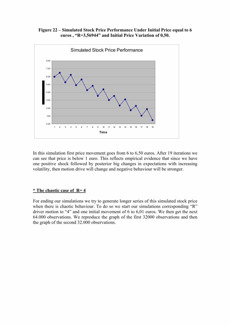
Figure 22 – Simulated Stock Price Performance Under Initial Price equal to 6 euros , “R=3,56944” and Initial Price Variation of 0,50.
Simulated Stock Price Performance
0.00
1.00
2.00
3.00
4.00
5.00
6.00
7.00
8.00
1 2 3 4 5 6 7 8 9 10 11 12 13 14 15 16 17 18 19
Time
In this simulation first price movement goes from 6 to 6,50 euros. After 19 iterations we can see that price is below 1 euro. This reflects empirical evidence that since we have one positive shock followed by posterior big changes in expectations with increasing volatility, then motion drive will change and negative behaviour will be stronger. * The chaotic case of R= 4 For ending our simulations we try to generate longer series of this simulated stock price when there is chaotic behaviour. To do so we start our simulations corresponding “R” driver motion to “4” and one initial movement of 6 to 6,01 euros. We then get the next 64.000 observations. We reproduce the graph of the first 32000 observations and then the graph of the second 32.000 observations.
Figure 23 – Simulated Stock Price Performance Under Initial Price equal to 6
euros , “R=4,00” and Initial Price Variation of 0,01 (First 32.000 observations).
Simulated Stock Price Performance
4.00
4.50
5.00
5.50
6.00
6.50
7.00
7.50
8.00
8.50
9.00
Time
Figure 24 – Simulated Stock Price Performance Under Initial Price equal to 6 euros , “R=4,00” and Initial Price Variation of 0,01 (Second 32.000 observations).
Simulated Stock Price Performance
4.00
5.00
6.00
7.00
8.00
9.00
10.00
11.00
12.00
1
1135
2269
3403
4537
5671
6805
7939
9073
1020
7
1134
1
1247
5
1360
9
1474
3
1587
7
1701
1
1814
5
1927
9
2041
3
2154
7
2268
1
2381
5
2494
9
2608
3
2721
7
2835
1
2948
5
3061
9
3175
3
Time
Stoc
k M
arke
t Pric
e
If we change the initial movement of 6 to 6,01 for 6 to 6,02 euros the behaviour comes more volatile as we expect. We reproduce the graph of the first 32.000 observations and then the graph of the second 32.000 observations.
Figure 25 – Simulated Stock Price Performance Under Initial Price equal to 6 euros , “R=4,00” and Initial Price Variation of 0,02 (First 32.000 observations).
Simulated Stock Price Performance
4.00
4.50
5.00
5.50
6.00
6.50
7.00
7.50
8.00
8.50
9.00
1
1126
2251
3376
4501
5626
6751
7876
9001
1012
6
1125
1
1237
6
1350
1
1462
6
1575
1
1687
6
1800
1
1912
6
2025
1
2137
6
2250
1
2362
6
2475
1
2587
6
2700
1
2812
6
2925
1
3037
6
3150
1
Time
Stoc
k M
arke
t Pric
e
Figure 26 – Simulated Stock Price Performance Under Initial Price equal to 6 euros , “R=4,00” and Initial Price Variation of 0,02 (Second 32.000 observations).
Simulated Stock Price Performance
4.00
5.00
6.00
7.00
8.00
9.00
10.00
11.00
12.00
1
1138
2275
3412
4549
5686
6823
7960
9097
1023
4
1137
1
1250
8
1364
5
1478
2
1591
9
1705
6
1819
3
1933
0
2046
7
2160
4
2274
1
2387
8
2501
5
2615
2
2728
9
2842
6
2956
3
3070
0
3183
7
Time
Stoc
k M
arke
t Pric
e
Conclusion. Our work here focus on the possible explanation of technical analysis view in the environment of nonlinear dynamics. To do so, we explain very quickly the foundation terms of technical analyisis beguining with Dow Theory and going to the Elliot Waves. Then we look at the foundations of nonlinear theory and chaotic theory with the example of Feigenbaum (1983) work with the nonlinear logistic equation. Our research, looking for some transformations of logistic nonlinear equation shows us that, since we state that market movements are generated in a strech and fold process, this equation can explain Fibonacci movements completely, showing that 0,618 and 1,618 gold numbers are one simplest consequence of nonlinear dynamics. This discovery, to our knowledge, is revolutionary and can give new support to technical analysis movement explanation and prediction, joining fractal, chaotic and technical analysis in one theoretical point of view. However we are cautious about our discoveries and we state that much work remains to be done. But this will be one of our future and we expect others working research.
REFERENCES Adler, R.J., R.E. Feldman and M.S. Taqqu ,1998, A Practical Guide to Heavy Tails, Boston, Birkhauser. Alexander, S. S. ,1961, Price Movements in Speculative Markets : Trends or Random Walks , Industrial Management Review 2, 7-26. Allen, F. e G. Gorton ,1993, Churning Bubbles , The Review of Economic Studies 60, 813-836. Attanasio,P O. ,1991, Risk Time_Varying Second Moments and Market Efficiency , Review of Economic Studies 58, 479-494. Barberis, N. , A. Schleifer and R. Vishny ,1998, A Model of Investor Sentiment, Journal of Financial Economics 49, 307-345. Barnsly, M. ,1988, Fractals Everywhere, San Diego, Academic Press. Belkacem, L., J. Lévy Véhel and C. Walter ,1996, CAPM, Risk and Portfolio Selection in "Stable" Markets", Rapport de Recherche, 2776, INRIA. Beran, J. ,1992, Statistical Methods For Data With Long-Range Dependence, Statistical Science 7, 404-427. Berliner, L. M. ,1992, Statistics, Probability and Chaos , Statistical Science 7, 69-122. Bollerslev,T. ,1986, Generalized Autoregressive Conditional Heteroscedasticity, Journal of Econometrics 31, 373-399. Bollerslev, T. ,1987, A Conditionaly Heteroskedastic Time Series Model For Speculative Prices and Rates of Return, Review of Economics and Statistics 69 , 542-547. Brock, W. ,1986, Distinguishing Random and Deterministic Systems : Abridged Version , Journal of Economic Theory 40,168-195. Brock, W. , W. D. Dechert e J. Scheinkman ,1987, A Test For Independence Based on The Correlation Dimension . In Dynamic Economic Modelling , Barret, W., E. Berndt e E. White ( eds ). Cambridge University Press, Cambridge. Brock, W., J. Lakonishok e B. LeBaron ,1992, Simple Technical Trading Rules and The Stochastic Properties of Stock Returns, The Journal of Finance 47, 1731-1763.
Brothers, K.M., W. H. DuMouchel and A.S. Paulson ,1983, Fractiles of the Stable Laws", Technical Report, Renssealaer Polytechnic Institute, Troy. Camerer, C. ,1989, Bubbles and Fads in Asset Prices : A Review of Theory and Evidence, Journal of Economic Surviews ( March 1989 ), 3-41. Chatterjee, S. and M. R. Yilmaz ,1992, Chaos, Fractals and Statistics, Statistical Science 7, 49-121. Cochrane, J. H. ,1991, Volatility Tests and Efficient Markets : A Review Essay, Journal of Monetary Economics 27, 383-417. Engle, R. F. ,1982, Autoregressive Conditional Heteroscedasticity With Estimates of The Variance of U. K. Inflation, Econometrica 50, 987-1008. Engle, R. F. and T. Bollerslev ,1986, Modelling The Persistence of Conditional Variances, Econometric Reviews 5, 1-50. Engle, R. F. and G. González-Rivera ,1991, Semiparametric ARCH Models,Journal of Business & Economic Statistics 9, 345-359. Fama, Eugene F. ,1965, The behaviour of stock-market prices, Journal of Business 38,34-105. Fama, E. ,1970, Efficient Capital Markets : A Review of Theory and Empirical Work, The Journal of Finance 25, 383-416. Fama, Eugene F. ,1976, Foundations of Finance, New York, Basic Books. Fama, E. e K. R. French ,1988, Permanent and Temporary Components of Stock Prices, Journal of Political Economy 96, 246-273. Fama, E. ,1991, Efficient Capital Markets: II, The Journal of Finance (December 1991),1575-1613. Fama, E. and K. R. French ,1993, Common Risk Factors in the Returns on Stocks and Bonds, Journal of Financial Economics 33, 3-56. Feigenbaum, M. J. ,1983, Universal Behavior in Nonlinear Systems, Physica 7D, 16-39. Francis, J. C. ,1986, Investments: Analysis and Management, New York, Mcgraw-Hill. French, K. R. and R Roll ,1986, Stock Return Variances : The Arrival of Information and The Reaction of Traders, Journal of Financial Economics 19, 5-26. French, K. R. , G. W. Schwert and R. F. Stambaugh ,1987, Expected Stock Returns and Volatility, Journal of Financial Economics 19, 3-29.
Frost, A.J. and R. R. Prechter, 1996, Elliot Wave Principle: Key to Market Behavior, Georgia, New Classics Library. Grassberger, P. and I. Procaccia ,1983, Measuring The Strangeness of Strange Attractors, Physica 9D,189-208. Haugen, R. ,1990, Modern Investment Theory", London, Prentice-Hall International Editions. Hsieh, D.A. ,1991, Chaos and Nonlinear Dynamics: Application to Financial Markets, The Journal of Finance 46, 1839-1877. Jegadeesh, N. ,1990, Evidence of Predictable Behavior of Security Returns, The Journal of Finance 45, 881-898. Kaheman, D. A. Tverskey ,1979, Prospect Theory: An Analysis of Decision Under Risk, Econometrica 47, 263-291. Kandell, Shmuel and Robert F. Stanbaugh ,1996, On The Predictability of Stock Returns: An Asset-Allocations Perspective, Journal of Finance 51(2), 385-424. Koutmos, G., C. Negakis and P. Theodossiou ,1993, Stochastic Behavior of The Athens Stock Exchange, Journal of Applied Financial Economics 3,119-126. Lamoureux, C.G. and W. D. Lastrapes ,1990, Persistence in Variance , Structural Change and The GARCH Model, Journal of Business & Economic Statistics 8, 225- 234. Lin, Weng-Ling, Robert F. Engle and Takatoshi Ito ,1994, Do Bulls and Bears Move Across Borders? International Transmission of Stock Returns and Volatility, Review of Financial Studies 7, 507-538. Lintner, John ,1965, The Valuation of Risky Assets and the Selection of Risky Investments in Stock Portfolios and Capital Budgets, Review of Economics and Statistics 47(1),13-37. Lo, A. W. and A. Mackinlay ,1988, Stock Market Prices do Not Follow Random Walks : Evidence From a Simple Specification Test, The Review of Financial Studies 1, 41-66. Lo, A. W. ,1991, Long Term Memory in Stock Market Prices, Econometrica 59, 1279- 1313. Lorenz, H.-W. ,1989, Nonlinear Dynamical Economics and Chaotic Motion. Springer Verlag eds. Macdonald, R. and D. Power ,1992, Persistence in U.K. Stock Market Returns: Some Evidence Using High-Frequency Data, Journal of Business Finance & Accounting 19, 505-513.
Maheu, J. M. and T. H. McCurdy ,2004, News Arrival, Jump Dynamics and Volatility Components for Individual Stock Returns, The Journal of Finance 59, 755-793. Mandelbrot, Benoit ,1963, The variation of certain speculative prices, Journal of Business 36, 394-419. Mandelbrot, B. and J. Wallis ,1968, Noah, Joseph and Operational Hydrology, Water Resources Research 4, 909-918. Mandelbrot, B. ,1972, Statistical Methodology For Non-Periodic Cycles : From Covariance to R/S Analysis, Annals of Economic and Social Measurement 1, 259-290. Mandelbrot, B. ,1982, The Fractal Geometry of Nature. W.H. Freeman eds. Mandelbrot, Benoit ,1997, Fractals and Scaling in Finance, New York, Springer Verlag. Mankwin, N.G., D. Romer and M. D. Shapiro ,1991, Stock Market Forecastability and Volatility : A Statistical Appraisal, Review of Economic Studies 58, 455-477. Markowitz, Harry M. ,1952, Portfolio Selection, Journal of Finance 7, 77-91. Markowitz, Harry M. ,1959, Portfolio Selection: Efficient Diversification of Investments, New York, Wiley. Markowitz, Harry M. ,1987, Mean-Variance Analysis in Portfolio Choice and Capital Markets, New York, Basil Blackwell. Markowitz, Harry M. ,1999, The Early History of Portfolio Theory: 1600-1960", Financial Analysts Journal 55, 5-16. Mayfield, E.S. and B. Mizrach ,1992, On Determining The Dimension of Real- Time Stock Price Data, Journal of Business & Economic Statistics 10, 367-374. Mcculloch, J. ,1978, Continuous Time Processes With Stable Increments, Journal of Business 51, 601-619. Mills, T.C. ,1993, Is There Long Term Memory in U.K. Stock Returns ?, Applied Financial Economics 3, 303-306. Mossin, Jan ,1966, Equilibrium in a Capital Asset Market, Econometrica 34(4),768-783. Nelson, D.B. ,1991, Conditional Heteroskedasticity in Asset Returns : A New Approach , Econometrica 59, 347-370. Neuman, Von J. and Oskar Morgenstern ,1953, Theory of Games and Economic Behavior, Princeton N.J., Princeton University Press.
Osborne, M.F.M. ,1964, Brownian Motion in The Stock Prices. Paul Cootner eds. ( M I T 1964 ). Pesin, J.B. ,1977, Characteristic Lyapunov Expoents and Smooth Ergodic Theory, Russian Mathematical Survey 32, 55-114. Peters, Edgar E. ,1991, Chaos and Order in The Capital Markets, New York, John Wiley & Sons. Pring, M. J. , 1991, Technical Analysis Explained, New York, McGraw-Hill,Inc. Rhea, R. ,1932, Dow Theory, New York, Barrons. Ross, S. ,1976, The Arbitrge Theory of Capital Asset Pricing, Journal of Economic Theory 13, 341-360. Samorodnitsky, Gennady and Murad S. Taqqu, 1994, Stable Non-Gaussian Random Processes - Stochastic Models With Infinite Variance, New York, Chapman & Hall. Sharpe, William F. ,1964, Capital Asset Prices: A Theory of Market Equilibrium Under Conditions of Risk, Journal of Finance 19(3), 425-442. Sharpe, William F. ,1966, Mutual Fund Performance", Journal of Business 39(1), 119-138. Sharpe, William F. ,1991, Capital Asset Prices With and Without Negative Holdings, Journal of Finance 64, 489-509. Scheinkman, J. and B. LeBaron ,1989, Nonlinear Dynamics and Stock Returns, Journal of Business 62, 311-337. Sewell, S.P., S.R.Stansell, I. Lee and M.-S.Pan ,1993, Nonlinearities in Emerging Foreign Capital Markets, Journal of Business Finance & Accounting 20, 237- 248. Shiller, R. ,1981, The Use of Volatility Measures in Assessing Market Efficiency, The Journal of Finance 36, 291-304. Shiller, R. ,1988, The Probability of Gross Violations of a Present Value Variance Inequality ", Journal of Political Economy 96,1089-1092. Shiller, R. ,1989, Market Volatility. The M.I.T. Press eds. Soares, Vasco J. S. ,1997, A (in)Eficiência dos Mercados Bolsistas de Acções, Porto, Vida Económica. Topol, R. ,1991, Bubbles and Volatility of Stock Prices : Effect of Mimetic Contagion", The Economic Journal 101, 786-800. Tverskey, A. ,1969, Intransitivity of Preferences, Psychological Review 76, 31-48.
Vaga, T. ,1991, The Coherent Market Hypothesis, Financial Analysts Journal (December/January). West, K.D. ,1988, Bubbles, Fads and Stock Price Volatility Tests: A Partial Evaluation" , The Journal of Finance 42, 63-74. Willey, T. ,1992, Testing For Nonlinear Dependence in Daily Stock Indices, Journal of Economics and Business 44, 63-74. Wolf, A.S., J.B. Swinney and H.L. Vastano ,1985, Determining Lyapunov Expoents From a Time Series ", Physica 16D ( July 1985 ), 285-317. Zarrowin, P. ,1990, Size, Seasonality and Stock Market Overreaction ", Journal of Financial and Quantitative Analysis 25, 113-125.