SCENARIO 1: NO FARM DAMS OR WATERCOURSE EXTRACTIONS .......................................................... 11
SCENARIO 2: CURRENT ESTIMATE OF DEMAND – WITHOUT LOW-FLOW RELEASES ................................ 11
WATER USE DATA ....................................................................................................................................................... 11
FARM DAMS DATA ...................................................................................................................................................... 11
WATER USE FROM FARM DAMS ................................................................................................................................. 13
Internal Annual Use Fraction ...................................................................................................................... 13
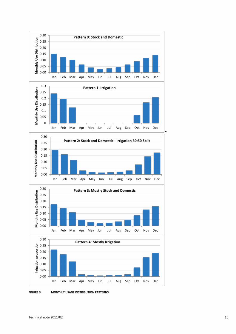
Definition of monthly usage distribution patterns ..................................................................................... 14
NET EVAPORATION FROM DAMS ............................................................................................................................... 16
SCENARIO 3, SCENARIO 4 AND SCENARIO 5 .......................................................................................... 19
DEMAND FROM FARM DAMS ..................................................................................................................................... 19
Variation of Usage from Lumped Dam Nodes where there is a combination of Licensed Irrigation Dams
and Non-licensed Stock and Domestic dams .............................................................................................. 20
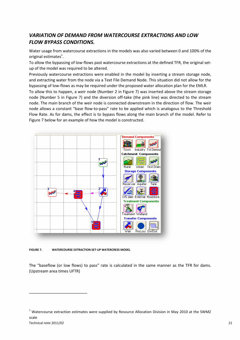
VARIATION OF DEMAND FROM WATERCOURSE EXTRACTIONS AND LOW FLOW BYPASS
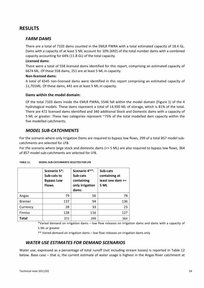
MODEL SUB-CATCHMENTS ......................................................................................................................................... 34
WATER USE ESTIMATES FOR DEMAND SCENARIOS .................................................................................................... 34
CATCHMENT WATER BALANCES ................................................................................................................................. 35
EFFECT OF LFB AND DEMAND SCENARIOS ON DAILY FLOW ....................................................................................... 37
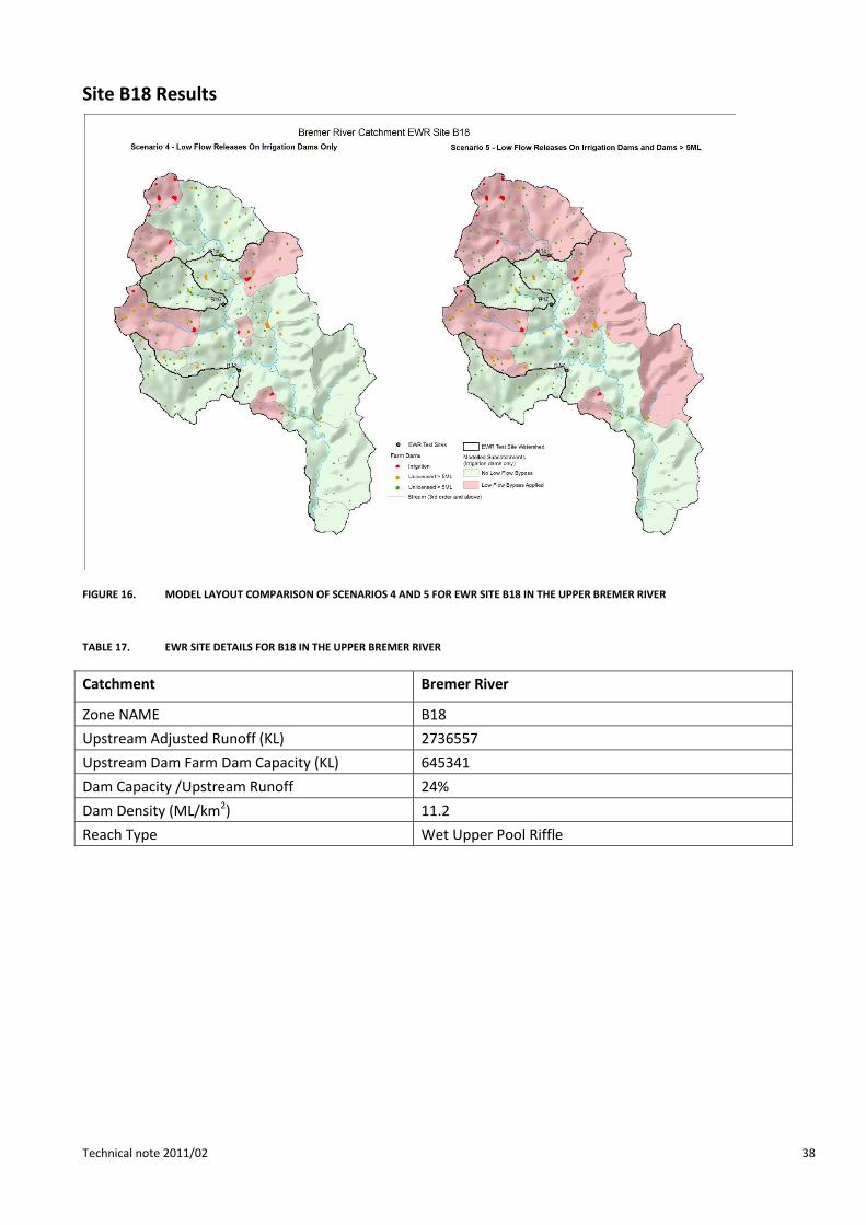
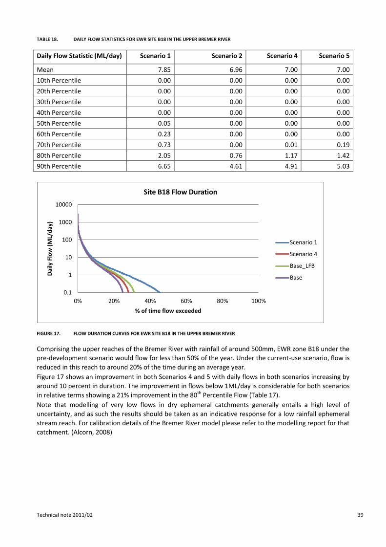
Site B18 Results ........................................................................................................................................... 38
Site F15 Results ........................................................................................................................................... 40
Figure 1. Unit Threshold Flow rates For the EMLR ..................................................................................................... 8
Figure 2. EMLR Prescribed Area showing model Domains ....................................................................................... 10
Figure 3. Monthly Usage Distribution Patterns......................................................................................................... 15
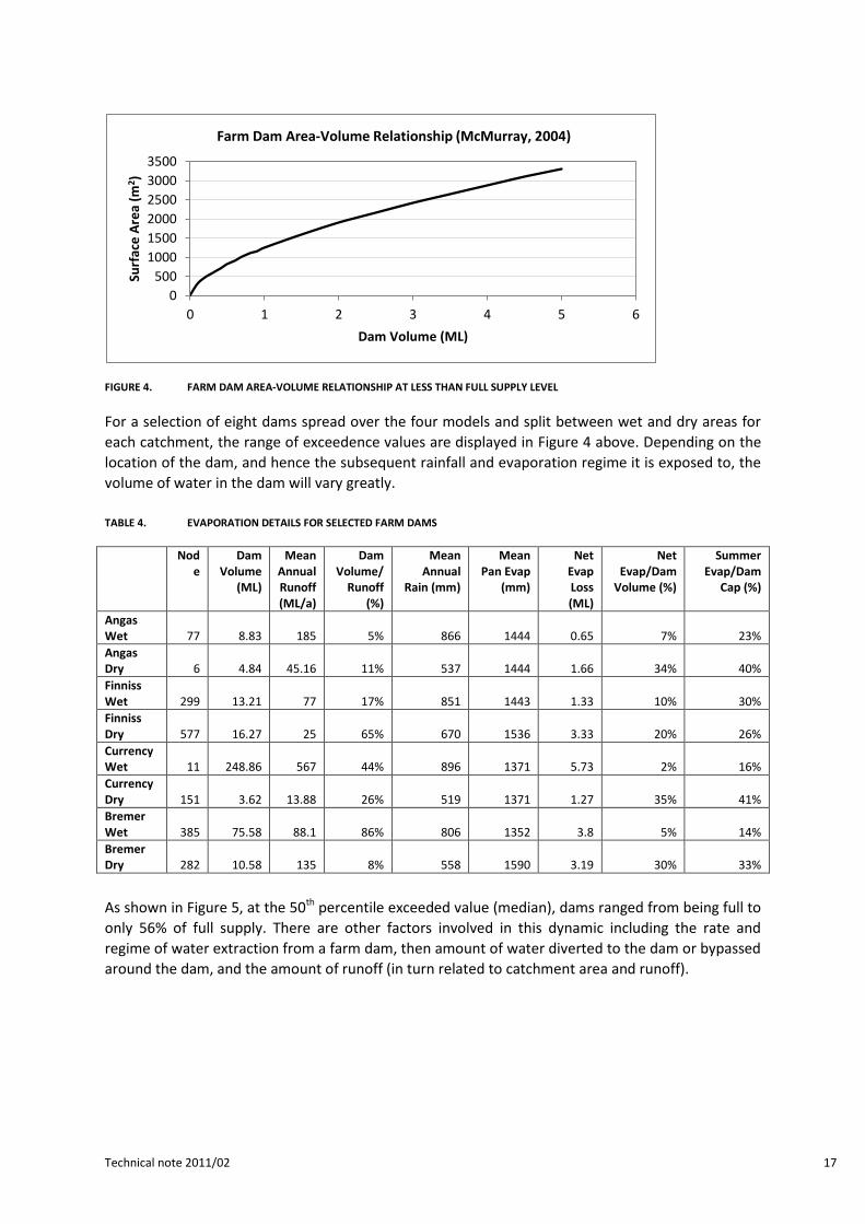
Figure 4. Farm dam area-volume relationship at less than full supply level............................................................. 17
Figure 5. Range of dam volume exceedences ........................................................................................................... 18
Figure 6. Mean monthly storage volume of EMLR Farm Dams ................................................................................ 18
Figure 7. Watercourse Extraction Set-up WaterCRESS Model .................................................................................. 21
Figure 8. Angas River Testing Sites and LFB Selection Scenario 4 ............................................................................ 25
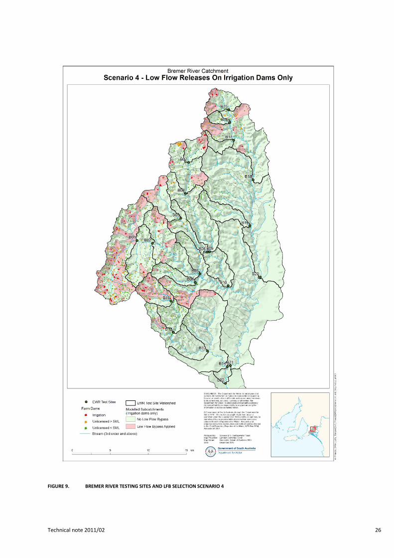
Figure 9. Bremer River Testing Sites and LFB Selection Scenario 4 .......................................................................... 26
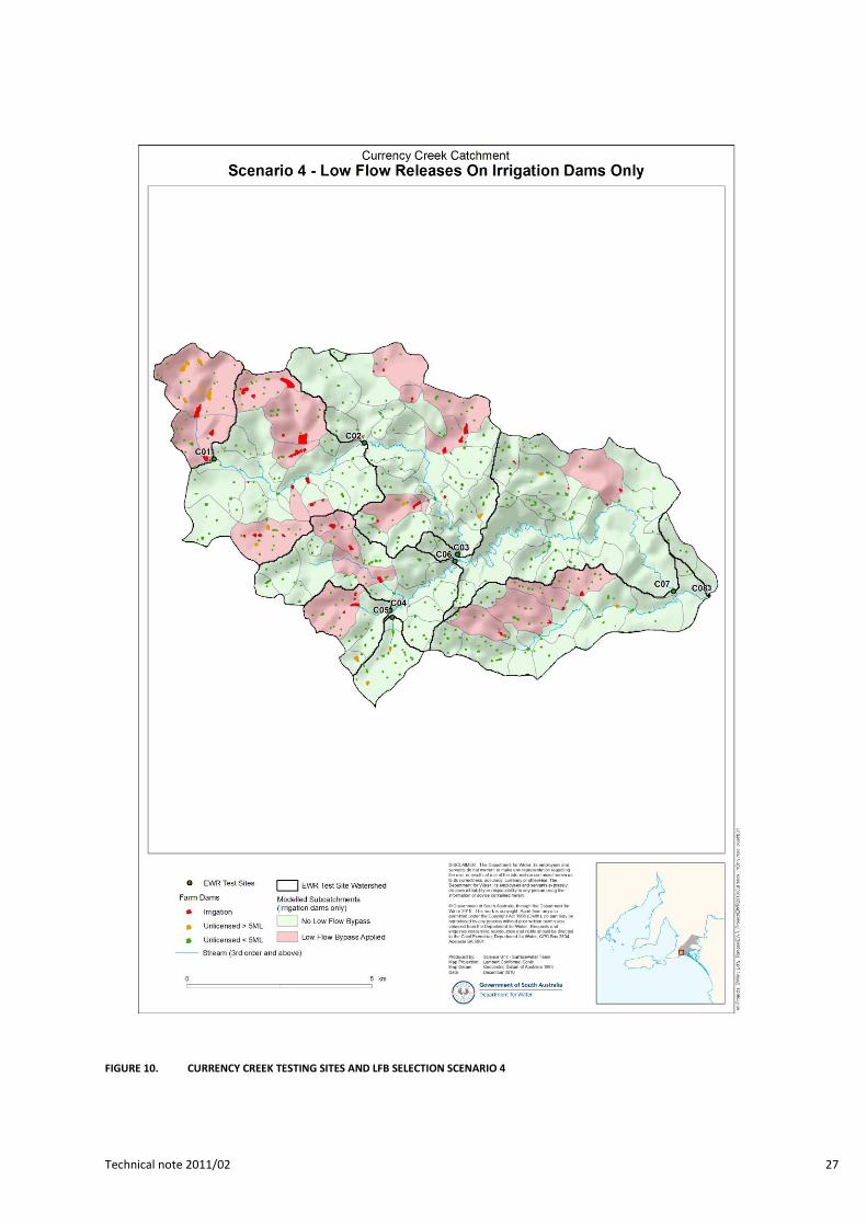
Figure 10. Currency Creek Testing Sites and LFB Selection Scenario 4 ....................................................................... 27
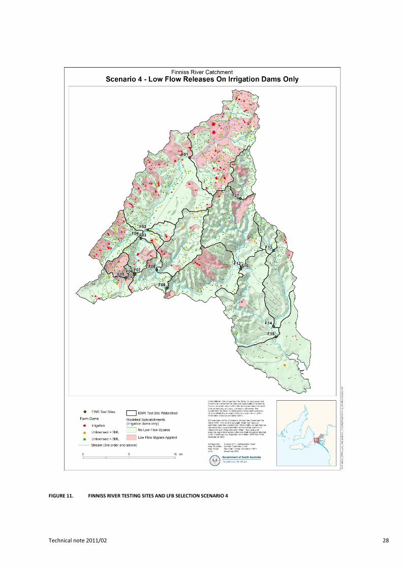
Figure 11. Finniss River Testing Sites and LFB Selection Scenario 4 ........................................................................... 28
Figure 12. Angas River Testing Sites and LFB Selection Scenario 5 ............................................................................. 29
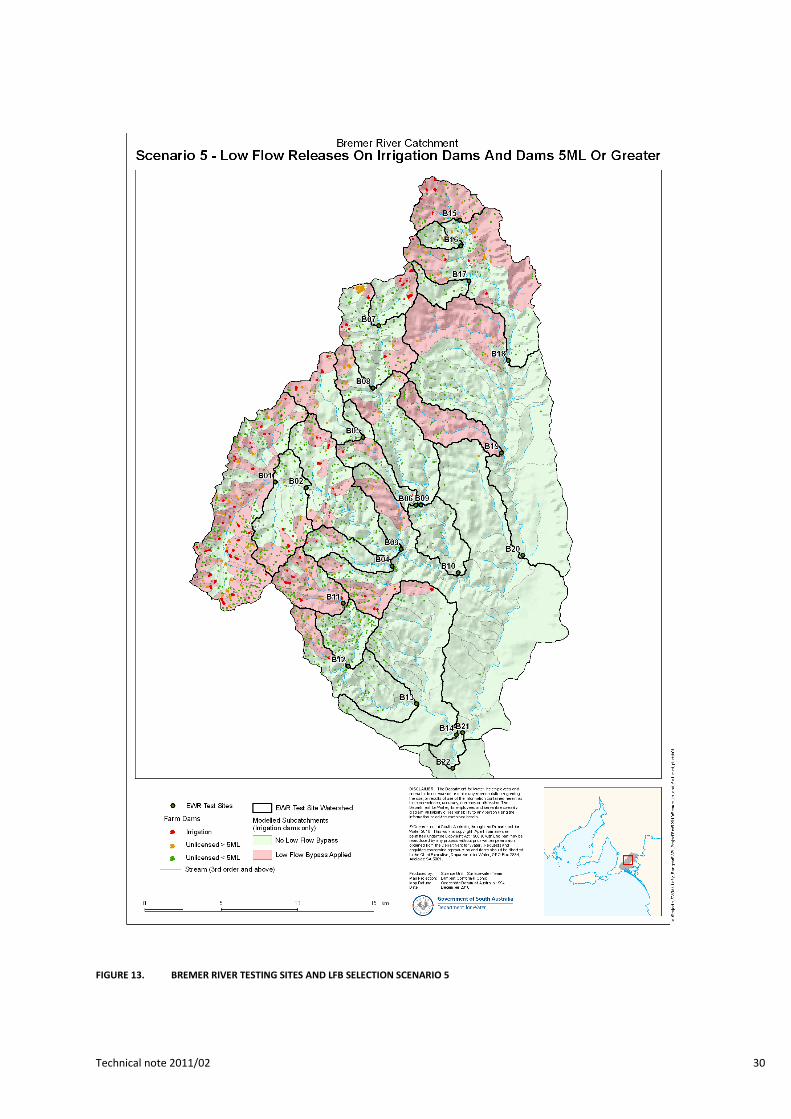
Figure 13. Bremer River Testing Sites and LFB Selection Scenario 5 .......................................................................... 30
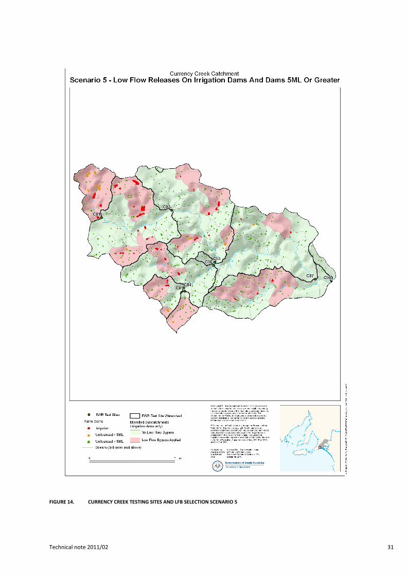
Figure 14. Currency Creek Testing Sites and LFB Selection Scenario 5 ....................................................................... 31
Figure 15. Finniss River Testing Sites and LFB Selection Scenario 5 ............................................................................ 32
Figure 16. Model Layout comparison of Scenarios 4 and 5 for ewr Site B18 in the Upper Bremer River .................. 38
Figure 17. Flow Duration Curves for EWR Site B18 in the Upper Bremer River .......................................................... 39
Figure 18. Model Layout comparison of Scenarios 4 and 5 for ewr Site F15 in the Lower Finniss River .................... 40
Figure 19. Flow Duration Curves for EWR Site F15 in the Lower FINNISS RIVER ........................................................ 41
Table of Tables
Table 1. Farm Dam Statistics for the EMLR .............................................................................................................. 12
Table 2. Farm Dam Statistics for the Five Modelled Catchments in the EMLR ........................................................ 12
Table 3. Usage patterns for Irrigation Proportion Ranges ...................................................................................... 14
Table 4. Evaporation details for selected farm dams .............................................................................................. 17
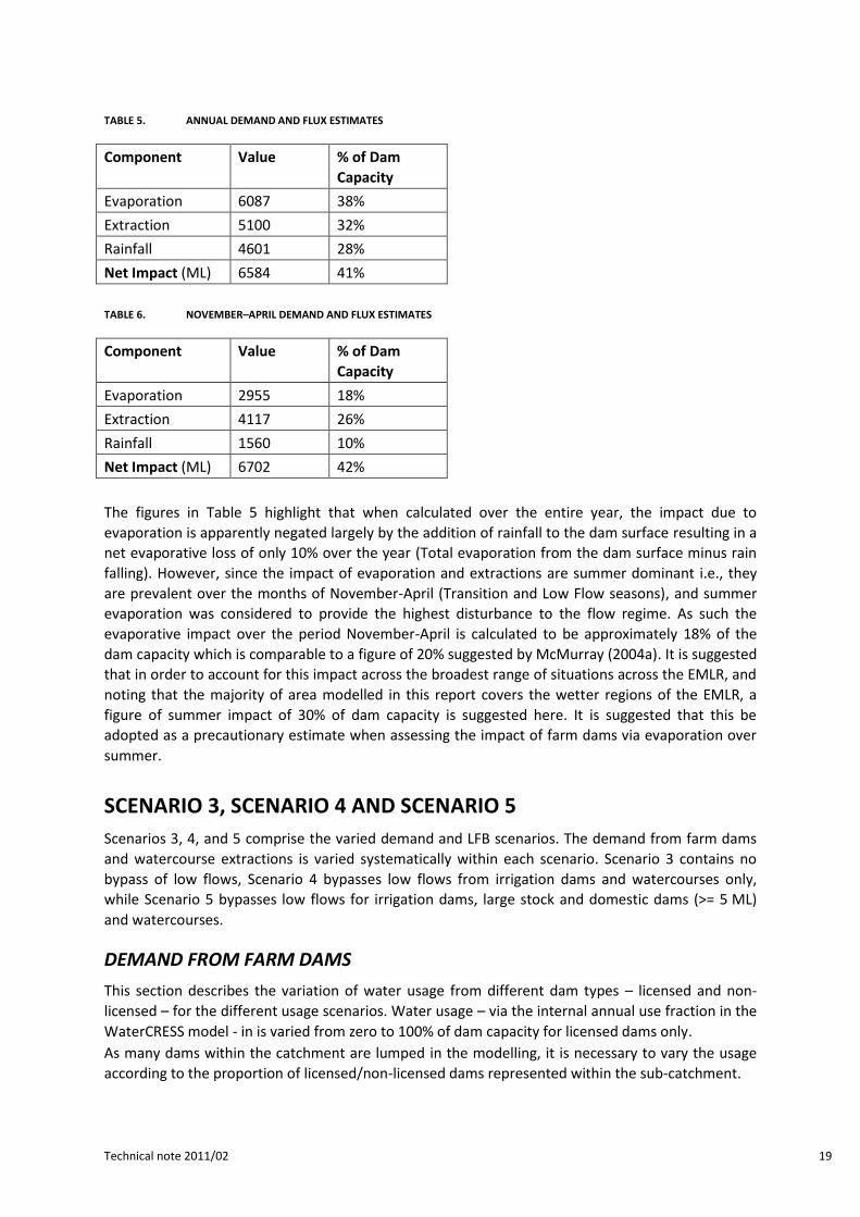
Table 5. Annual demand and flux estimates ............................................................................................................ 19
Table 6. November–April demand and flux estimates ............................................................................................ 19
Table 7. Example for a 50% Irrigation Proportion ................................................................................................... 20
Table 9. Sub-catchments Selected for low flow bypass ........................................................................................... 22
Table 10. List of Scripts to run EWR Scenario Analysis .............................................................................................. 23
Table 11. Model Sub-catchments Selected for LFB ................................................................................................... 34
Table 12. Water usage as percent of total Catchment Runoff for various Demand scenarios .................................. 35
Table 13. Angas River Catchment Water Balance ...................................................................................................... 36
Table 14. Bremer River Catchment Water Balance ................................................................................................... 36
Table 15. Currency Creek Catchment Water Balance ................................................................................................ 36
Table 16. Finniss River Catchment Water Balance .................................................................................................... 37
Table 17. EWR Site Details for B18 in the Upper Bremer River ................................................................................. 38
Table 18. Daily Flow Statistics for EWR Site B18 in the Upper Bremer River ............................................................ 39
Table 19. EWR Site Details for F15 in the Lower Finniss River ................................................................................... 40
Table 20. Daily Flow Statistics for EWR Site F15 in the Lower Finniss River .............................................................. 40
Technical note 2011/02 6
INTRODUCTION
AIM
The aim of this report is to summarise the work of the Science Monitoring and Information (SMI)
Division within the Department for Water (DFW) in undertaking surface water modelling of the
Eastern Mount Lofty Ranges (EMLR) Prescribed Surface Water Area (PSWA) for a range of water
usage and Low Flow Bypass scenarios.
The scenarios where Low Flow Bypass (LFB) occurs at: 1. All irrigation dams; and
2. All irrigation dam and all stock and domestic dams with a cease-to-flow storage volume of 5
megalitres (ML) or greater, and for a range of water demands from dams and watercourses.
This work was requested by the SA Murray-Darling Basin Natural Resources Management Board
(SAMDBNRMB), to provide input to the determination of Environmental Water Requirements (EWR)
for the EMLR.
SCOPE
The intended scope of this report is to document the techniques and assumptions used to model the
effect of low flow bypasses on farm dams, threshold flow rates on watercourse extractions and
varying levels of water demand from the existing network of surface water development. The
primary outcomes of this modelling are files containing modelled daily flow estimates for 63 testing
sites over 4 catchment models within the EMLR.
Additional outputs of this study are:
the automated generation of individual files describing the EWRs for each test site for each modelling
scenario
A collated spreadsheet containing summaries of all models and results for each site and scenario.
The daily hydrological models used in this study cover Bremer River (Alcorn, 2008), Angas River
(Savadamuthu, 2006), Finniss River (Savadamuthu, 2003) and Currency Creek (Alcorn, M., 2006).
BACKGROUND
This work forms a part of the ongoing work by the DFW to provide science support to the process of
Prescription in the Eastern Mount Lofty Ranges (EMLR) Prescribed Water Resources Area (PWRA).
This is the third in a series of hydrological reports for the EMLR, and provides a range of water use
and management options to the SAMDBNRMB, for the purpose of assessment of Environmental
Water Requirements (EWRs) and eventually the Environmental Water Provisions (EWPs).
The first of these reports (Alcorn et al, 2008) sets out the basic framework for calculating the
capacity of the surface water resource of the EMLR, with regard particularly to the impacts of farm
dams on streamflow. The second report (Alcorn, 2010), revisited the existing hydrological models,
updating farm dam data and climate data, and included the impact of existing watercourse
extractions. It also provided the framework for estimating the average impacts of plantation forestry
on the landscape as required through the Statewide Policy Framework (SA Government, 2009).
This report describes the scenario modelling requested by the SAMDBNRMB, and any changes made
to the models since the estimates reported in DFW (2010). The outputs from this study are the
modified daily time series at a series of test sites throughout the EMLR.
Technical note 2011/02 7
Technical note 2011/02 8
LOW FLOW RELEASE RATES
At the time of writing, it was likely that intended policy options for the EMLR Water Allocation Plan
(WAP) will include the installation of some form of low-flow bypass device on licensable farm dams,
and watercourse extractions, or the requirement to release low flows to the environment some
other way. This report investigates the effect of including those releases. For licensable farm dams in
the models flows are bypassed around the dam, and for watercourse extractions only water above
the Unit Threshold Flow Rate (UTFR) may be extracted.
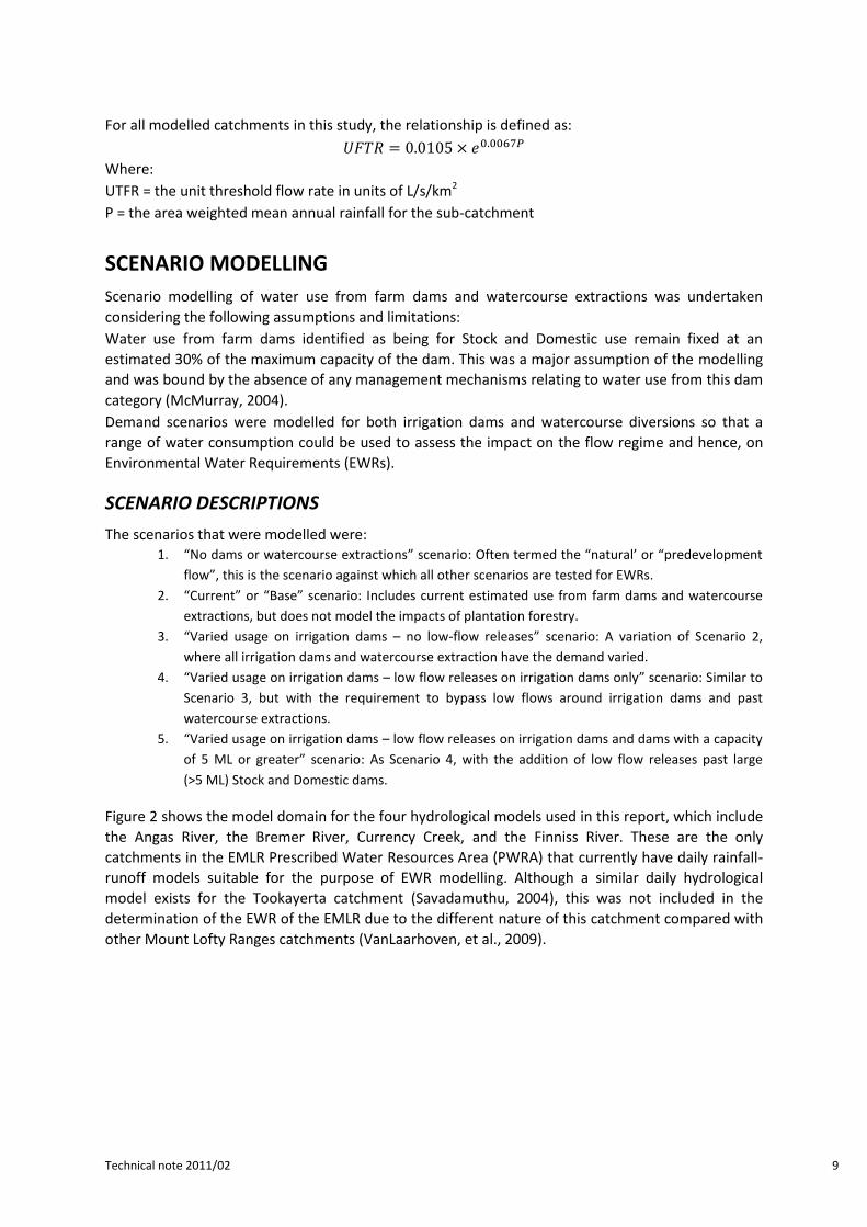
UNIT THRESHOLD FLOW RATES
The Unit Threshold Flow Rate (UTFR) is defined as the rate of flow per square kilometre of
catchment at or below which water must not be diverted or collected by a dam, wall or other
structure, and is expressed in litres/second/km2. This rate was set to be equivalent to the rate of
daily flow that is exceeded or equalled for 20% of the flowing period of the catchment. It is
calculated by removing the zero flow days from the record and calculating the daily flow that is
exceeded 20% of the time.
As calculating this value is not possible at the location of each and every dam or every watercourse
extraction or diversion, a regional curve was constructed using streamflow data from all available
gauging stations in the Mount Lofty Ranges and the corresponding rainfall in the catchment. This
curve is shown in Figure 11 below. This allows a variable UTFR to be used for any location in the
catchment, to be defined based upon the rainfall upstream of the dam or watercourse extraction in
question.
The rationale for choosing this threshold was that it is approximately equivalent to the definition of
a “T1 Fresh”, in the Environmental Water Requirements flow metrics (Van Laarhoven and van der
Wielen, 2009), and is relatively simple to calculate from measured streamflow data.
The UTFR for a dam (or a watercourse extraction) can be calculated by taking the mean annual
rainfall upstream of the dam (or the watercourse) location and finding that point on the x-axis of the
chart below, and finding the corresponding UTFR on the y-axis. Multiply the UTFR by the catchment
area above the dam (or the watercourse extraction) to give the location specific Threshold Flow Rate
(TFR) in litres per second.
FIGURE 1. UNIT THRESHOLD FLOW RATES FOR THE EMLR
0
0.5
1
1.5
2
2.5
3
3.5
4
4.5
5
0 100 200 300 400 500 600 700 800 900 1000
Un
it T
hre
sho
ld F
low
Rat
e (
l/s/
km2 )
Mean Annual Rainfall (mm)
Unit Threshold Flow Rates (L/Sec/Km2)
Technical note 2011/02 9
For all modelled catchments in this study, the relationship is defined as:
Where:
UTFR = the unit threshold flow rate in units of L/s/km2
P = the area weighted mean annual rainfall for the sub-catchment
SCENARIO MODELLING
Scenario modelling of water use from farm dams and watercourse extractions was undertaken
considering the following assumptions and limitations:
Water use from farm dams identified as being for Stock and Domestic use remain fixed at an
estimated 30% of the maximum capacity of the dam. This was a major assumption of the modelling
and was bound by the absence of any management mechanisms relating to water use from this dam
category (McMurray, 2004).
Demand scenarios were modelled for both irrigation dams and watercourse diversions so that a
range of water consumption could be used to assess the impact on the flow regime and hence, on
Environmental Water Requirements (EWRs).
SCENARIO DESCRIPTIONS
The scenarios that were modelled were: 1. “No dams or watercourse extractions” scenario: Often termed the “natural’ or “predevelopment
flow”, this is the scenario against which all other scenarios are tested for EWRs.
2. “Current” or “Base” scenario: Includes current estimated use from farm dams and watercourse
extractions, but does not model the impacts of plantation forestry.
3. “Varied usage on irrigation dams – no low-flow releases” scenario: A variation of Scenario 2,
where all irrigation dams and watercourse extraction have the demand varied.
4. “Varied usage on irrigation dams – low flow releases on irrigation dams only” scenario: Similar to
Scenario 3, but with the requirement to bypass low flows around irrigation dams and past
watercourse extractions.
5. “Varied usage on irrigation dams – low flow releases on irrigation dams and dams with a capacity
of 5 ML or greater” scenario: As Scenario 4, with the addition of low flow releases past large
(>5 ML) Stock and Domestic dams.
Figure 2 shows the model domain for the four hydrological models used in this report, which include
the Angas River, the Bremer River, Currency Creek, and the Finniss River. These are the only
catchments in the EMLR Prescribed Water Resources Area (PWRA) that currently have daily rainfall-
runoff models suitable for the purpose of EWR modelling. Although a similar daily hydrological
model exists for the Tookayerta catchment (Savadamuthu, 2004), this was not included in the
determination of the EWR of the EMLR due to the different nature of this catchment compared with
other Mount Lofty Ranges catchments (VanLaarhoven, et al., 2009).
Technical note 2011/02 10
FIGURE 2. EMLR PRESCRIBED AREA SHOWING MODEL DOMAINS
Technical note 2011/02 11
SCENARIO 1: NO FARM DAMS OR WATERCOURSE EXTRACTIONS
The “No dams or watercourse extractions” scenario: Often termed the “natural’ or “predevelopment
flow”, this is the scenario against which all other scenarios are tested for EWRs.
This scenario is modelled by removing all farm dams and watercourse extractions from the model.
Note that modelled urban areas (Bremer and Angas models) are not removed as this modelling is
focussed only on the impact of farm dams and watercourse extractions.
SCENARIO 2: CURRENT ESTIMATE OF DEMAND – WITHOUT LOW-FLOW RELEASES
The current or “Base” Case scenario includes current estimated use from farm dams and
watercourse extractions, but does not model the impacts of plantation forestry. The results of this
scenario are not discussed directly, but are considered as part of the range of results reported in
Scenario 3, which encompass a broader range of demand estimates. Described in this section are the
assumptions around farm dam water usage and extractions from streams.
WATER USE DATA
Water use across the modelled catchments in the EMLR is currently represented in the hydrological
models by:
farm dam extractions,
watercourse diversions and extractions, and
flood irrigation.
FARM DAMS DATA
Farm dam water use is dominant in the highlands of the EMLR and is categorised within this report
as either: 1. Irrigation: A dam from which water is used to irrigate land for commercial purposes. As this type of
water use is controlled under the WAP, dam types in this category are also termed “licensed dams”.
The terms “Licensed dam(s)” and “irrigation dam(s)” are used interchangeably in this report.
2. Stock and Domestic: A dam from which water is taken to water stock or for domestic use. As this type
of water use is not proposed to be controlled by the draft WAP, dam types in this category are also
termed non-licensed dams. The terms “Stock and Domestic dam(s)” and “non-licensed dam(s)” are
used interchangeably in this report.
Data describing farm dams in the EMLR is based on a combination of previously captured data and
updated estimates of licensed dam capacities and locations. Licensed dam locations and cease to
spill capacities of those dams were provided to this analysis by DFW's Water Planning and
Management Division (WPMD) derived from detailed land and water use surveys carried out over
the prescription period.
The remaining dams are categorised as Non-licensed dams. These dams were captured from high
resolution aerial photography covering the period 2003-2005.
Farm dam capacity estimates are derived in the following way using the following methods in order
of preference/accuracy: 1. Estimate from field survey or design calculations. Usually provided to the DFW as part of the land and
water use survey, and this is considered the better of the dam capacity estimates. Many licensed
dams are estimated using this method.
Technical note 2011/02 12
2. Estimated using field survey of dam wall height and surface area. The formula used derive volume
using this method is:
a. ( ) ( ) ( )
3. Estimated using surface area derived from aerial photography using the following formula:
a.
i. V= 0.0002A1.25
b. For A >= 15 000
i. V = 0.0022A
These formulas and their application are described in McMurray (2004).
Summary
Dams in the EMLR Prescribed Water Resources Area:
There are an estimated total of 7103 dams in the EMLR PWRA with a total capacity of 18.4 GL. Dams
with a capacity of at least 5 ML account for around 10% of the total number dams (692) with a
combined capacity accounting for 64% (11,828 ML) of the total volume.
TABLE 1. FARM DAM STATISTICS FOR THE EMLR
Dam Types Count Capacity
Licensed < 5 ML 307 559
Licensed > 5 ML 251 6115
Total Licensed 558 6674
SD < 5 ML 6104 5988
SD > 5 ML 441 5713
Total SD 6545 11701
Total Dams 7103 18375
Dams within the model domain in this report
Of the total 7103 dams inside the EMLR PWRA, 5546 (78%) fall within the model domain (Figure 2) of
the 4 hydrological models. These dams represent a total of 14,930 ML of storage, which is 81% of
the total storage. There are 472 licensed dams identified and 340 additional Stock and Domestic
dams with a capacity of 5 ML or greater.
These two categories represent ~75% of the total modelled dam capacity within the four modelled
catchments.
Table 2 below shows the dam statistics by modelled catchment.
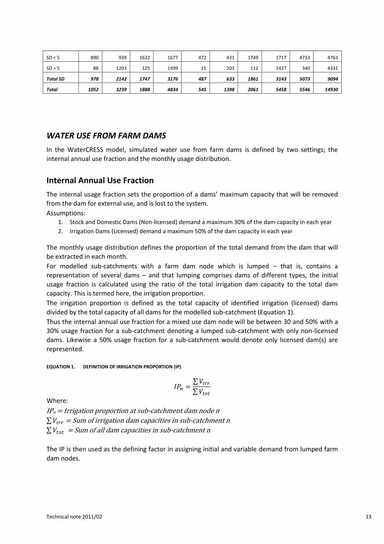
TABLE 2. FARM DAM STATISTICS FOR THE FIVE MODELLED CATCHMENTS IN THE EMLR
Catchment Angas River Bremer River Currency Creek Finniss River Total
(Model Domain)
Dam Type Count Volume Count Volume Count Volume Count Volume Count Volume