AD-A252 689 TECHNICAL REPORT BRL-TR-3363 BRL MODELING RHA PLATE PERFORATION BY A SHAPED CHARGE JET_ DTIC ELECTE 1 JUL•3 1992 flfl MARTIN N. RAFTENBERG SAO 7 JUNE 1992 'Orihtuai oontalns c1o1o -. , plates% All DTIC reproduct- Ions w111 be In black and white* AMOVED FOR PUBLTC PRMEASE DOIRMON IS UNLIMarD. U.S. ARMY LABORATORY COMMAND BALLISTIC RESEARCH LABORATORY ABERDEEN PROVING GROUND, MARYLAND 92-18162 9 2 4 •• ,. t!11111i~ ll,~lll tt IIIl
Transcript
AD-A252 689
TECHNICAL REPORT BRL-TR-3363
BRLMODELING RHA PLATE PERFORATION
BY A SHAPED CHARGE JET_
DTICELECTE 1JUL•3 1992 flfl
MARTIN N. RAFTENBERG SAO
7 JUNE 1992'Orihtuai oontalns c1o1o -. ,plates% All DTIC reproduct-Ions w111 be In black andwhite*
AMOVED FOR PUBLTC PRMEASE DOIRMON IS UNLIMarD.
U.S. ARMY LABORATORY COMMAND
BALLISTIC RESEARCH LABORATORYABERDEEN PROVING GROUND, MARYLAND
92-181629 2 4 •• ,. t!11111i~ ll,~lll tt IIIl
NOTICES
Destroy this report when it is no longer needed. DO NOT return it to the originator.
Additional copies of this report may be obtained from the National Technical Information Service,U.S. Department of Commerce, 5285 Port Royal Road, Springfield, VA 22161.
The findings of this report are not to be construed as an official Department of the Army position,unless so designated by other authorized documents.
The use of trade names or manufacturers' names in this report does not constitute indorsementof any 'commercial product.
-DISCJLAIMli NOT WE
THIS DOCUMENT IS BEST
QUALITY AVAILABLE. THE COPY
FURNISHED TO DTIC CONTAINED
A SIGNIFICANT NUMBER OF
COLOR PAGES WHICH DO NOT
REPRODUCE LEGIBLY ON BLACK
AND WHITE MICROFICHE.
Form Approved
REPORT DOCUMENTATION PAGE Fo0MB Aro04-0
g ainr " a r.v,rmia tnn e aata neecae ana c Ioetinj a"c 'e..- :r -' r '-'a cc -::,'t ~ao'z rs r Cps Sea~,.- 51 3" Z.I: Scom nc nf)mtflc, -, uar g r~3r sgge~st-n icr recuctra -,n rO .ýs nuro" -eaa aýWý's Se' es C- reno,aie ic, rr"f-a!,cn ooe' co-s a'nc Qe.ris i2 - "ersor
Da,.S H qtýa.. Sj'te 12C4 ;. qtcrý -. 122^~2-43C2 and ! t-- O 'fi -- " drZ '.:: - o-'Clw Rea~C.. P-::eez Cý7C4-1'881 V.a~s,nc.7, C 0SC31. AGENCY USE ONLY (Leave blank) 2. REPORT DATE 3. REPORT TYPE AND DATES COVERED
I June 1992 Fmal, May 89-Mar 92
4. TITLE AND SUBTITLE 5. FUNDING NUMBERS
Modeling RHA Plate Perforation by a Shaped Charge Jet PR: 1L162618AH80
6. AUTHOR(S)
Martin N. Raftenberg
7. PERFORMING ORGANIZATION NAME(S) AND ADDRESS(ES) 8. PERFORMING ORGANIZATIONREPORT NUMBER
9. SPONSORING / MONITORING AGENCY NAME(S) AND ADDRESS(ES) 10. SPONSORING MONITORINGAGENCY REPORT NUMBER
U.S. Army Ballistic Research Laboratory BRL-TR-3363ATIN: SLCBR-DD-TAberdeen Proving Ground, MD 21005-5066
11. SUPPLEMENTARY NOTES
12a. DISTRIBUTION / AVAILABILITY STATEMENT 12b. DISTRIBUTION CODE
Approved for public release; distribution is unlimited.
13. ABSTRACT (Maximum 200 words)
Models for metal failure by tensile voids and shear bands are presented and inserted into hydrocode EPIC-2. Eachmodel consists of an onset criterion and a post-onset prescription on stresses. The resulting code is used to simulate anexperiment involving perforation of a 13.0-mm-thick RHA plate by the leading particle of an OFHC copper jetproduced by firing a shaped charge warhead at long standoff. Quantities evaluated from the experiment and comparedwith computational results include the final hole radius averaged over the plate's thickness, the final hole shape, thetime required for hole formation, the net mass lost by the plate, and the location of voids and shear bands in thefinalplate cross section.
Three parameters are varied in the calculations. One of these is associated with each of the two failure models,and the third with the slideline erosion algorithm. With neither failure model or with only the tensile failure modelactive, the computed hole is too small and its formation is completed prematurely. However, when both failure modelsare active, reasonable agreement with the experiment is obtained for a range of parameter values.
Three problems are repeated with a finer mesh. The degree of mesh sensitivity is quantified.
LJLIST OF SYMBOLS ........................................... 127
DISTRIBUTION LIST .......................................... 131
SMvalabilily Cou.!s
Avail o,iclorDist Spcial0-l
INTENTIONALLY LEFT BLANK.
iv
LIST OF FIGURES
Figure Page
1. Experimental Setup for Rd. 10771 .................................. 38
2. Flash Radiographs of the Jet at 161.5 and 181.4 ps After Explosive Initiation 39
3. Flash Radiographs of the Jet and RHA Plate at 181.0 and 226.3 ps AfterExplosive Initiation ... ...................................... 40
4. Enlargement of Flash Radiograph of the Jet and RHA Plate at 226.3 ps AfterExplosive Initiation ....................................... 41
5. Photograph of the Perforated Plate's Entrance Surface ................... 42
6. Photograph of the Perforated Plate's Exit Surface ...................... 43
7. Perforation Hole in RHA Plate Fitted by a Circle ...................... 44
8. Construction of Radial Slices to be Removed From Perforated Plate ....... 45
9. Removal of Five Radial Slices From Perforated Plate ................. 46
10. Five Radial Slices From the Perforated Plate ....................... 47
11. Digitized Boundary of a Slice From the Perforated Plate and Calculation ofthe Throat Radius and r~F% From Rd. 10771 ................... 48
12. Flash Radiographs at Various Times From Rds. 4190 and 4189 .......... 49
13. Five-Parameter Geometric Model for the Leading Jet Particle ............ 50
14. The Jet Particle Model Fitted to the Radiograph at 8.6 ps Before Impact .... 51
15. The Initial Mesh Used in Sections 5, 7, and 8 ....................... 52
16. Mesh Plot at 3.01 ps After Impact for Problem I-C ..................... 53
17. Mesh Plot at 4.02 ps After Impact for Problem I-C ..................... 54
18. Mesh Plot at 500.04 ps After Impact for Problem I-C ................... 55
19. Mesh Plot at 10.02 ps After Impact for Problem I-C, With DisembodiedNodes of Ejecta and Debris Included ......................... 56
V
Figure Page
20. Mesh Boundary at 500.04 ps and Calculation of F,, From Problem I-C .... 57
21. Computed 7r,& vs. Poa for Problem Series I ...................... 58
22. Mesh Plot at 500.00 ps After Impact for Problem I-E ................... 59
23. Mass Lost From Target Plate vs. Time for Problem Series I ............. 60
24. Micrograph of a Fracture Surface Formed by Void Coalescence in theRHA Target Plate of Rd. 10771 .............................. 61
25. Micrograph of a Shear Band in the RHA Target Plate of Rd. 10771 ....... 62
26. Micrograph of a Crack That Extends Along a Shear Band in the RHA Plate ofRd. 10771 ... .......................................... 63
27. Sketch Showing Locations of Prominent Voids and Shear Bands in a RadialSlice From the RHA Plate of Rd. 10771 ........................ 64
28. Mesh Plot at 1.02 ps After Impact for Problem 11-C .................... 65
29. Mesh Plot at 3.02 ps After Impact for Problem I1-C .................... 66
30. Mesh Plot at 500.00 ps After Impact for Problem 11-C ................. 67
31. Mesh Plot at 500.05 ps After Impact for Problem II-A ................. 68
32. Mesh Plot at 500.03 ps After Impact for Problem 11-B ................. 69
33. Mesh Plot at 500.02 ps After Impact for Problem 11-D ................. 70
34. Mesh Plot at 500.00 is After Impact for Problem II-E ................. 71
35. Computed rhole vs. lProde for Problem Series I ...................... 72
36. Mass Lost From Target Plate vs. Time for Problem Series I ............ 73
37. The Deviatoric-Stress Reduction Function Used With the Shear BandFailure Model ............................................ 74
38. Computed rh/oe vs. .ro& With A,-t a Parameter for Problem SeriesIII Through VIII .......................................... 75
vi
Figure Page
39. Computed r-.,,• vs. AEf7j With ePode a Parameter for Problem SeriesIII Through VIII ............................................ 76
40. Mesh Plot at 1.03 ps After Impact for Problem Ill-B .................. 77
41. Mesh Plot at 2.01 ps After Impact for Problem III-B .................. 78
42. Mesh Plot at 3.01 ps After Impact for Problem III-B .................. 79
43. Mesh Plot at 4.03 ps After Impact for Problem rI-B .................. 80
44. Mesh Plot at 5.00 ps After Impact for Problem rI-B .................. 81
45. Mesh Plot at 10.01 ps After Impact for Problem HI-B ................... 82
46. Mesh Plot at 20.04 ps After Impact for Problem II-B ................... 83
47. Mesh Plot at 50.04 ps After Impact for Problem HI-B .................. 84
48. Mesh Plot at 100.06 ps After Impact for Problem HI-B ................ 85
49. Mesh Plot at 150.05 ps After Impact for Problem HII-B ................ 86
50. Mesh Plot at 200.06 ps After Impact for Problem HI-B .................. 87
51. Mesh Plot at 250.04 ps After Impact for Problem HI-B ................ 88
52. Mesh Plot at 300.06 ps After Impact for Problem HI-B .................. 89
53. Mesh Plot at 450.05 ps After Impact for Problem II-B ................ 90
54. Mesh Plot at 500 02 ps After Impact for Problem HI-B ................ 91
55. Mesh Plot at 500.00 ps After Impact for Problem IV-C .................. 92
56. Mesh Plot at 500.06 ps After Impact for Problem V-D ................ 93
57. Mesh Plot at 500.04 ps After Impact for Problem VI-E ................ 94
58. Mass Lost From Target Plate vs. Time for Problem Series III ............ 95
59. Mass Lost From Target Plate vs. Time for Problem Series IV ............ 96
vii
Page
60. Mass Lost From Target Plate vs. Time for Problem Series V ............ 97
61. Mass Lost From Target Plate vs. Time for Problem Series VI ............ 98
62. Mass Lost From Target Plate vs. Time for Problem Series VII ........... 99
63. Mass Lost From Target Plate vs. Time for Problem Series VIII ............ 100
64. Computed AM vs. cP,£o With Afaa a Parameter for Problem Series IIIThrough VIII .. ......................................... 101
65. Computed AM vs. Afau With oEP a Parameter for Problem Series IIIThrough VIII .. ......................................... 102
66. The Initial Mesh Used in Section .) .............................. 103
67. Mesh Plot at 3.00 ps After Impact for Problem I-C(R) ................. 104
68. Mesh Plot at 4.00 ps After Impact for Problem I-C(R) ................. 105
69. Mesh Plot at 500.02 ps After Impact for Problem I-C(R) ............... 106
70. Mass Lost From Target Plate vs. Time for Problems I-C and I-C(R) ....... 107
71. Mesh Plot at 1.00 ps After Impact for Problem II-C(R) .................. 108
72. Mesh Plot at 3.01 ps After Impact for Problem II-C(R) ................. 109
73. Mesh Plot at 500.00 ps After Impact for Problem II-C(R) .............. 110
74. Mass Lost From Target Plate vs. Time for Problems II-C and II-C(R) ...... 111
75. Mesh Plot at 1.01 ps After Impact for Problem nI-B(R) ................ 112
76. Mesh Plot at 2.01 ps After Impact for Problem III-B(R) ................ 113
77. Mesh Plot at 3.01 ps After Impact for Problem III-B(R) ................ 114
78. Mesh Plot at 4.00 ps After Impact for Problem HI-B(R) ................ 115
79. Mesh Plot at 5.02 ps After Impact for Problem III-B(R) ................ 116
80. Mesh Plot at 10.02 ps After Impact for Problem mI-B(R) ............... 117
viii
Figure Page
81. Mesh Plot at 20.02 ps After Impact for Problem III-B(R) ............... 118
82. Mesh Plot at 50.03 ps After Impact for Problem II-B(R) ............... 119
83. Mesh Plot at 100.01 ps After Impact for Problem IlI-B(R) .............. 120
84. Mesh Plot at 200.02 ps After Impact for Problem II-B(R) ............... 121
85. Mesh Plot at 500.01 ps After Impact for Problem HI-B(R) ................. 122
86. Mesh Boundary at 500.01 ps and Calculation of rh,& for Problem III-B(R) 123
87. Mass Lost From Target Plate vs. Time for Problems 11-B and llI-B(R) ..... 124
ix
LNTENrIQNALLY LEFT BLANK.
LIST OF TABLES
Table Page
1. Parameter Values for the Leading Jet Particle's Geometric Model ...... 34
2. Material Parameter Values for the Metals ....................... 34
3. Results From Problem Series I ............................... 35
4. Results From Problem Series II .............................. 35
5. Results From Problem Series III Through VIII .................... 36
6. Results With the Refined Mesh .............................. 37
7. CPU Times on a Cray X-MP/48 for Six Problems ................. 37
xi
INTENTioNALLY LEFT BLANK.
xl'
ACKNOWLEDGMENTS
Thomas W. Wright and Michael J. Scheidler of the U.S. Army Ballistic Research
Laboratory (BRL), Aberdeen Proving Ground, MD, and Howard Tz. Chen of the Naval
Surface Warfare Center, Silver Spring, MD, provided assistance in developing the shear band
model. Claire D. Krause, formerly of BRL, obtained the micrographs in Figures 24, 25, and
26 and produced the sketch in Figure 27. Robert A. Stryk and Gordon R. Johnson of Afliant
Techsystems, Inc. in Brooklyn Park, MN, gave helpful comments on EPIC-2 coding.
Jonas A. Zukas of BRL provided an insightful review of this report.
The author thanks Elaine Kessinger and Doris Cianelli of Nomura Enterprise Inc. for their
assistance in preparing the figures.
xiii
INTENTIONALLY LEFT BLANK.
xiv
1. INTRODUCTION
The problem of rolled homogeneous armor (RHA) plate perforation by a
shaped charge jet is one of ongoing interest to the U.S. Army Ballistic Research
Laboratory. With the advent of supercomputers, the problem can now be analyzed
with more detail and greater realism than has previously been possible. The present
study presents an analysis of a single case, that of a particular shaped charge
warhead fired at normal incidence and long standoff into a 13.0-mm-thick plate.
The range firing is described in Section 2. Section 3 follows with the evaluation
from experiment of three quantities pertaining to the perforated target plate that
provide convenient benchmarks for hydrocode calculations. As preparation of input
to the hydrocode, the geometry of the jet's leading particle is analyzed from
radiographs in Section 4. Features of EPIC-2 (Johnson and Stryk 1986), the
hydrocode used in this study, are reviewed in Section 5. Of particular interest is its
eroding slideline feature. Also, a series of problems using only features contained
in the 1986 version of EPIC-2 are presented as an initial modeling effort in this
section. Section 6 presents evidence for the failure mechanisms of tensile voids and
shear bands, as observed by applying microscopy to specimens removed from the
perforated plate. Section 7 describes a model for failure due to tensile voids that
has been installed into EPIC-2. A series of problems employing this added feature is
discussed. Section 8 describes a model for failure by shear bands which has also
been installed. Six series of problems are run using this model in conjunction with
that for tensile voids. Results from these series are compared with experiment. In
Section 9 one problem from each of Sections 5, 7 and 8 is rerun with a finer mesh in
order to observe the sensitivity of results to the gridding. Section 10 summarizes
the findings and suggests follow-up work.
2. RANGE FIRING
The shaped charge warhead used has a conical copper liner with a 420 apex
angle, an 81.28-mm outer-diameter base, and a 1.91-mm wall thickness. The
explosive fill used is Composition-B. It is fired at a standoff of 15.23 charge
diameters (C.D.) into a 13.0-mm-thick RHA plate. RHA is a medium-carbon,
quenched and tempered, martensitic steel. Its allowable ranges of chemical
composition and heat treatment are specified in U.S. Department of Defense (1984).
The plate's cross-section is approximately square, with a 197-mm edge length. A
Brinell hardness number (BHN) of 364 for the entrance and exit surfaces is
obtained. Figure 1 shows the experimental setup, including the position and
orientation of four flash X-ray tubes. The round number is 10771 of Range 7A.
Figure 2 displays two flash radiographs on one film sheet, taken at 161.5 and 181.4
Its after explosive initiation. Figure 3 shows the images on the second sheet. These
apply at 181.0 and 226.3 gts after initiation. Figure 4 contains an enlargement of the
image at 226.3 its after initiation. This time corresponds to about 36 Pis after intial
impact with the plate. Figures 2 through 4 show the jet's leading particle to have
completely perforated the plate. The trailing particles are aligned with the leading
particle and pass through the hole that it has made.
3. THREE BENCHMARK QUANTITIES EVALUATED FROM
EXPERIMENT
The perforated plate's entrance surface is shown in Figure 5. Its exit surface is
presented in Figure 6. The plate's hole is reasonably circular, except for a single
notched region. Away from this notch, the hole is assumed to have been created
entirely by the jet's leading particle. This assumption is supported by the degree of
alignment in the jet's particles that was noted in the radiographs above. The hole is
fitted by a circle (Figure 7), and radii spaced at 25.70 are constructed (Figure 8).
Slices of plate material corresponding to five adjacent radii are removed (Figures 9
and 10). The boundary of the uppermost slice in Figure 10 is digitized to describe
the hole's profile (Figure 11).
Srholx is defined as the value determined from experiment of the final hole
boundary's radius averaged over the plate's thickness. The average radius of the
red surface in Figure 11 is determined by numerical integration of the digitized
coordinates. The result is a value of 18.2 mm for rh, so
= 18.2 mm (1)
This quantity will serve as a convenient benchmark by which to evaluate hydrocode
solutions. Two other quantities that will also serve this function are AMexP and
ex.9xý. AMexp is defined to be the experimentally-determined total mass lost by the
target plate. t.egxf• is the experimentally-determined time after initial impact at which
the plate has lost 95% of this mass. No data by which to evaluate AMexP and t.egxf•
2
were obtained from Round (Rd.) 10771.
Fortunately, two more recent experiments, Rds. 4189 and 4190 of Range 16, do
provide such data. In both of these experiments, the same shaped charge warhead
employed in Rd. 10771 was fired into an RHA plate at a standoff of 975 mm (12.0
C.D.) The impact conditions at this standoff are quite similar to those at 15.2 C.D.In both cases the entire jet has broken up into particles that have probably ceased to
stretch. Spacings between successive particles are greater at 15.2 C.D. than at 12.0
C.D., but Figures 3 and 4 establish that the fastest particles and probably mostparticles pass through the hole made by the first particle without contacting the
plate. The target plates in Rds. 4189 and 4190 had respective thicknesses of 12.6
and 12.8 mm, both close to the 13.0 mm value of Rd. 10771. Thus data from Rds.
4189 and 4190 are assumed transferrable to Rd. 10771.
In Rd. 4190 the plate was weighed before and after the firing to produce a
measurement of 136 g for AMeXP, so
AMeXP = 136 g (2)
A total of six flash radiographs was obtained from Rds. 4190 and 4189. As shown
in Figure 12, these radiographs visualize the debris patterns at 1.7, 18.2, 33.2, 73.9,
143.2 and 213.0 pts after initial impact. The three earliest views were obtained from
Rd. 4190, and the three latest from Rd. 4189. The first RHA fragments to form are
small and are seen to keep pace with the fastest moving jet particles. Much largerfragments appear at later times. In Section 8 distinct micromechanical mechanisms
will be suggested for these two classes of fragments. It seems from Figure 12 that
substantial material has separated from the plate subsequent to 73.9 pts after impact.A rough estimate for t.•'*s is therefore
t.9f- > 73.9 pts (3)
The difficulty with assigning a time of fragment separation from the target plate on
the basis of radiographs such as Figure 12 should be borne in mind, however. Such
radiographs directly show only the later time at which the separated fragment has
moved a noticeable distance from the plate.
3
4. LEADING JET PARTICLE DESCRIPTION
Figure 2 shows the leading jet particle at 161.5 and at 181.4 pts after initiation.
These times correspond to 28.5 and 8.6 p s before impact, respectively. Based on
these two images, the leading particle's impact velocity is determined to be 7.73
mm/As.
A cylindrical coordinate system is introduced, with its origin at the center of thetarget plate's entrance surface. Axial coordinate z measures distance from this
surface, with positive values in the region between the plate and the warhead's
original position. The digitized image of the jet's leading particle at 8.6 pls before
impact is mapped onto this cylindrical coordinate system by translation and rotation.The mapping is defined by three constraints: (i) and (ii) The particle's volume and
centroid location, when computed based on the portion on one side of the r= 0
centerline, agree with those computed using the portion on the other side of the
centerline. (iii) Following translation and rotation, the point on the digitized
boundary that intersects the centerline at the lowest z coordinate is assigned the
position z= 0, i.e., is placed in contact with the center of the plate's entrance
surface. In addition to producing a geometry on which to base input to an
axisymmetric hydrocode analysis, the mapping determines the particle's length,volume and centroid position to be 20.6 mm, 353.2 mm3 , and 7.97 mm above the
base, respectively.
A five-parameter model for the leading particle's geometry is shown in Figure
13. The model's length L,, volume Vp, and centroid position zp are expressed in
terms of its five parameters by
Lp = Lc + Ls + LB (4)
Vp = itRs 2 HLC + Ls + LBX (5)
4
1 [ i ] 12 ,I LC LB + Ls + I LC +L B+- S+IL 2 sIL 8+s+Lc+ LsiL 8 +L-i+ LB X
Zp 4 1 (6)3 Lc + Ls + LBX
3
where
2 1+ 12+ 3 -3 (7)
Lp. Vp and zp are assigned the values 20.6 mm, 353.2 mm 3, and 7.97 mm,
respectively, as evaluated above on the basis of a radiograph. Equations (4), (5)
and (6) can then be viewed as three equations in the five unknowns Lc, Ls, LB, Rs
and RB. A solution is obtained for Lc, Ls and LB in terms of Rs and RB.
Corresponding to a guess for the values of Rs and RB, the quantities Lc, Ls and LB
are evaluated and the model of Figure 13 is drawn. This procedure is applied
iteratively until a close visual fit to the jet particle's shape according to the
radiograph is obtained. The image in Figure 14, which corresponds to the values
for Lc, Ls, LB, Rs and RB that are listed in Table 1, is deemed to be an acceptable fit
to the radiograph.
5. EPIC-2 SIMULATIONS WITHOUT FAILURE MODELING
5.1 Features of EPIC-2. The 1986 version of Lagrangian hydrocode EPIC-2
(Johnson and Stryk 1986) is used to model the Rd. 10771 experiment. The two
metals, copper and steel, are both handled in the same fashion. Their dilatational
deformation is governed by the Mie- Gruineisen equation of state
p= (K4I+KA2 +K 3 9'3]1 2L1g + F(1 + .)e (8)
where
i ._ 1 (9)Po
5
p is pressure, or negative hydrostatic stress, p is current density, Po is undeformed
density, e is the internal energy per undeformed volume, and IF is the Gruneisen
coefficient. Values for K 1, K 2 , K 3 and F are presented for OFHC copper and for
304 stainless steel in Kohn's handbook (Kohn 1965). These parameter values are
displayed in Table 2, in which Kohn's values for austenitic 304 stainless steel have
been applied to martensitic RHA.
The distortional deformation of copper and steel is treated by means of a
plasticity model, which applies the von Mises yield condition as follows: At each
cycle, deviatoric Cauchy stress components Srr, Szz, s$0 and Srz are computed by
applying elastic shear modulus G to the total strain increment. Equivalent stress a
is then computed using
a= [(Srr 2 + Szz 2 + SOO 2 ) + 3S(2 20)
and is compared to the current flow stress y , a measure of the state of the
material. If a < ay, only elastic deformation occurs during that cycle and the
computed stress components are unaltered. If a _Ž ay, plastic, non-recoverable
deformation occurs as well as elastic. If a> cy , stresses are adjusted along a radial
path in stress space so that a becomes equal to ayy.
Flow stress ay is computed using the Johnson-Cook strength model (Johnson
and Cook 1983). According to this model, ay is a function of equivalent plastic
strain eP, equivalent plastic strain rate e", and homologous temperature T*. The
functional form is
y [A + B(EP)N [1+ C ln P I - (T*)M (11)
where
IDP DPLLJ.? 2 (12)33
and
t
EP= f 0dt (13)0
t is time and DP- is the plastic component of the rate of deformation tensor. T* isrelated to room temperature Tr and melting temperature T,. by
TTTr (14)
where T is the current temperature, computed using a thermodynamic relation.
Equation (11) expresses strain hardening, strain rate hardening, and thermal
softening as separate factors. Hardening is assumed to be isotropic. Constants G,A, B, N, C, M, Tr, and T.. are assigned their values presented for OFHC copper andfor 4340 steel by Johnson and Cook (1983). These values are listed in Table 2.
The slideline erosion algorithm of EPIC-2 enables the application of thisLagrangian hydrocode to problems in penetration mechanics. A description of this
essential feature is reserved for the next subsection, 5.2.
In addition the 1986 version of EPIC-2 contains a failure model, or algorithm
to cause stress reduction within a finite element subsequent to the local satisfactionof some onset criterion. This Johnson-Cook failure model is phenomenological and
was derived fit data from Hopkinson bar tests and quasi-static tensile tests
(Johnson and Cook 1985). Such tests involve relatively low strain rates, so the
model is judged to be inappropriate for the present application. In particulardescriptions in Johnson and Cook (1985) of damaged specimens contain no mention
of shear banding, which in Section 6 will be shown to constitute one of two
micromechanical mechanisms for material failure found to be operative in RHAspecimens from Rd. 10771. The other micromechanical mechanism is ductile voids,
which apparently was also active in the experiments of Johnson and Cook.
Nevertheless, the range of ambient conditions on strain rate and temperature were
indeed much smaller in their experiments than in Rd. 10771, so a much simpler
model for void failure will be utilized instead in this report.
5.2 Problem Series I. The axisymmetric mesh used in all calculations of this
section as well as Sections 7 and 8 is shown in Figure 15. It consists of three-nodetriangular elements. The copper projectile's mesh closely approximates the
7
geometry of the five-parameter model with parameter values listed in Table 1. It
contains 124 node points and 202 elements. The target's mesh approximates the
square steel plate by a circular disk with a thickness of 13.0 mm and a radius of
104.0 mm. Individual elements in the target are isosceles right triangles, the longest
edge of which has a length of 1.3 mm. This corresponds to ten layers of crossed
triangles through the target plate's thickness. The target's mesh irncludes 3200 of
these elements and 1691 node points.
The mesh contains two slidelines, both coincident with the projectile/target
interface. One slideline has the projectile's surface nodes serving as master nodes
and the target's surface nodes as slaves. In the other slideline this assignment is
reversed.
The erosion feature is operative for both slidelines. This allows an element
having one or more corner node on the master surface of the slideline to be
discarded from the problem in the sense that all stresses in the element are
thereafter set to zero. Since both copper projectile nodes and steel target nodes
alternately serve as master nodes for one of the two slidelines, the procedure
provides a means for modeling both projectile erosion and target hole formation.
EPIC-2 uses three criteria to trigger erosion of a given surface element. One
criterion is a user-supplied cutoff value for equivalent plastic strain, EPode. Another
is an angle cutoff, whereby none of the element's vertex angles is allowed to become
less than a certain acute value. These two criteria limit the degree of distortion in
the element. The third criterion discards a group of one or more elements that is
connected to the master surface by a single vertex node. This criterion is motivated
by the need to prevent such elements from crossing the slideline surface.
Following erosion of a slideline element, its three associated node points, to
which its entire mass has been lumped, remain in the problem. One or two may
become effectively disembodied from the remaining projectile or target. When this
occurs, those disembouied nodes are converted from master into slave nodes. They
subsequently interact with the remaining master surface and participate in
momentum transfer across the slideline. Furthermore, previously interior nodes that
now find themselves located on the master surface become identified as the
slideline's master nodes. EPIC-2's eroding slideline algorithm is described further
in Stecher and Johnson (1984).
8
In later sections of this report, two failure models will be developed to cause
stress reduction in el- .ients not necessarily located along the current slideline.
Before considering this additional feature, consider a series of five problems that are
run using only those features already discussed. It will be referred to as Problem
Series I. Erosion strain EPerode is assigned the values 0.25, 0.50, 0.75, 1.25 and 2.00,
as listed in Table 3. Each problem begins at the instant of initial impact and is run
until 500 gis after impact. Mesh plots for Problem I-C, for which Perode equals 0.75,
are shown at 3.01, 4.02, and 500.04 Vs after impact in Figures 16, 17, and 18,respectively. Perforation has occurred between 3.01 and 4.02 Ais after impact. This
implies a penetration velocity between 3.23 and 4.32 mm/gts averaged over the
course of perforation.
Figure 19 shows the mesh from Problem I-C at 10 ts after impact, with the
nodes disembodied by slideline erosion indicated. Each of these nodes is assigned by
means of -ts color to one of the four categories: "target debris", "projectile debris",
"target ejecta", and "projectile ejecta". "Target debris" denotes disembodied nodes
of RHA material having a negative axial velocity 4. According to the coordinate
system of Figure 19, nodes with negative axial velocity travel in the same direction
as the jet particle and away from the original (before detonation) warhead position.
"Target ejecta" denotes disembodied nodes of RHA material having a positive axial
velocity, or traveling towards the original warhead position. Similarly, "projectile
debris" and "projectile ejecta" denote disembodied nodes of copper material with a
negative and a positive axial velocity, respectively.
Now consider results for the average hole radius at 500 gts after initial impact,
rhole. Figure 20 redraws the boundary of the target mesh of Figure 18. The portion
of this boundary associated with the perforation hole boudary is shown in red.
rhole is computed from Figure 20 by numerical integration of nodal coordinates
along this red section. The result for Problem I-C is 11.0 mm, substantially smaller
than the experimental result of 18.2 mm obtained from Figure 11. Results for rhole
from Problem I-C and the other four problems in the series are listed in Table 3 and
plotted vs. perode in Figure 21. The computed values for rhole are seen to increase
with increasing eprode. However, even for an Peode of 2.00 (Problem I-E), the
computed rhole of 13.9 mm is still substantially smaller than the experimental result.
The mesh of the target plate at 500 ps for Problem I-E is presented in Figure 22.
The large value of F-erode for this problem has allowed highly distorted elements to
9
be retained in the final mesh. This consideration leads to the decision not to apply
values of EProde in excess of 2.00, even though the trend in Figure 21 suggests that
such values might yield more realistic results for rhole.
Figure 23 plots the total mass that has eroded from the target plate vs. time
after impact for the five problems of Problem Series I. These total masses are
computed for a given time step by summing the masses of all steel elements that
have eroded at or before that time step. Results for AM, the total mass lost at 500
Its, and t.95, the time at which the plate has lost 0.95 AM of mass, can be obtained
from Figure 23. These results are collected in Table 3. LM results are rather
insensitive to EProde for Eerode equal to 0.25, 0.50, and 0.75. However, by an eProde
of 1.25, AM is seen to decrease with increasing eerode. This last trend is in contrast
to the increase in hole radius rhole with increasing Ederoje that was noted above. This
discrepancy between relationships of rhole and AM to EPZrode is resolved by a
comparison of the mesh plots in Figures 18 and 22. Hole growth is seen to have
been accompanied by the removal of fewer RHA elements in Problem I-E than in
Problem I-C. Instead, in Problem I-E many highly distorted elements have been
retained, leading to much radial compression of material near the hole "throat", or
most narrow cross-section, and to the formation of prominent lips at the entrance
and exit surfaces along the hole boundary. AM values for the five problems are all
much smaller than the experimental value of 136 g in Equation (2). This is
consistent with the fact that computed rhoke values are all smaller than the
measurement from Rd. 10771. Results for t. 9 5 in Table 3 are all substantially
smaller than the experimental lower bound of Equation (3).
The results from Problem Series I can be summarized as follows: For the mesh
of Figure 15 and for the parameter Perode varied simultaneously for both slidelines in
the range of 0.25 to 2.00, (i) rhole is smaller than the measurement from Rd. 10771,
(ii) AM is smaller than the measurement from Rd. 4190, and (iii) t95 is smaller than
the range indicated by Rds. 4190 and 4189. In short the computed holes are too
small, and their growths are completed prematurely.
10
6. EXPERIMENTAL OBSERVATIONS OF VOIDS AND SHEAR BANDS
At this point the perforated target plate of Rd. 10771 is studied further to assessthe micromechanical processes that it has undergone. RHA specimens are extractedfrom the perforated plate in the vicinity of the hole. They are then polished, etched
in 2% Nital, and examined using photomicroscopy and scanning electron
microscopy. Figure 24 displays a fracture surface that has been formed by voidcoalescence. Figure 25 shows a shear band with a characteristic 6-4m width, whileFigure 26 displays a crack that runs along part of a shear band's length. From thesefigures, it is concluded that fracture, and therefore fragmentation of RHA, are
associated with the two phenomena of voids and shear bands that result from
interaction with the jet.
The extracted slice of RHA target plate from Rd. 10771 that was photographed
to produce Figure 11 is now polished and examined with an optical microscope atmagnifications up to 1000X. The goal is to observe the locations of prominent voids
and shear bands in the final target plate cross-section. Here "prominent" is used tomean "observable with an optical microscope at 1000X magnification." The results
are sketched in Figure 27. Voids and shear bands are seen to be concentrated in thehole boundary's region that is located near the plate's midsurface and that protrudes
into the hole to form the throat. At least nine large, discrete voids and eleven shearbands can be observed in this region. Each shear band contacts either a void, the
hole boundary, or in some cases both. Two or three prominent shear bands are alsoobserved near the intersection of the hole boundary with the plate's entrance
surface.
7. EPIC-2 SIMULATIONS WITH THE TENSILE FAILURE MODEL
7.1 The Tensile Failure Model. The voids in the RHA plate noted in Figure 24art assumed to have nucleated and grown under the action of a tensile stress field.A tensile failure model to simulate effects of these voids at the finite element level is
now developed and added to EPIC-2. In contrast to the slideline erosion algorithm,
this tensile failure model will be applied to target and jet-particle elements
throughout the domain, both on and off the slideline. The model consists of two
parts: (i) a failure onset criterion and (ii) a prescription for post-onset stressreduction.
11
The onset criterion of the tensile failure model is developed first. The
approximately spherical shape of individual voids in the photomicrograph of Figure
24 suggests that their growth was driven by the spherically symmetric portion of the
stress tensor, namely the hydrostatic stress. Pressure is negative hydrostatic stress,
defined in terms of Grr, czz and G;0, the radial, axial and circumferential normal
components of the Cauchy stress by
P 3 rr+ GZZ+ gee] (15)
The RHA specimen of Figure 24 was removed from the remaining target plate
in the vicinity of the perforation hole. The figure therefore displays material at
about 19 mm from the shot line. The observation just made regarding
spheroidally-shaped voids is assumed to apply throughout the RHA target plate.
This last assumption is challengeable in that during the perforation process, RHA
material that was originally located closer to the shot line presumably experienced
much larger values for such field variables as strain, strain rate and temperature
than did the material of Figure 24. However, the assumption receives some support
from publications by researchers at SRI International (e.g., Barbee et al. 1972,
Seaman et al. 1976). These publications have established that this general situationof fractures formed by coalescing spheroidal voids occurs quite commonly in shock
loaded metals. They call such fracture "ductile", as opposed to their category of
"brittle" fracture, which is characterized by planar cracks. In particular Barbee et al.
(1972) has shown the situation to be at least sometimes applicable to OFHC copper.
On this basis a pressure criterion for tensile failure onset will be applied to the
copper jet particle as well as to the RHA.
In an element of either RHA target material or OFHC copper jet material, the
onset of tensile failure is assumed to occur when the pressure, which at a given time
step is constant in an element, becomes less than or equal to a negative-valued
material parameter Pfail, i.e.,
P < Pfail < 0 (16)
For each metal, Pfail is taken to be a constant, independent of both the local current
values and the histories of all field variables.
12
The prescription for post-onset behavior will be considered next. Once the
failure onset criterion of Equation (16) is met in an element, that element is no
longer allowed to support hydrostatic tensile stress or deviatoric stresses. The
element is only allowed to support hydrostatic compression. This involves
modifications to the EPIC-2 hydrocode which at each time step affect all elements
that have either then or at some previous time step satisfied Equation (16). For all
such elements, deviatoric stresses are not computed, and positive hydrostatic stress
values that result from evaluation of the Mie- Gruneison equation of state are
altered and set to zero.
Note that this post-onset prescription involves the instantaneous reduction to
zero of certain stress components once the tensile failure onset criterion has been
met. The prescription therefore ignores the possiblity for gradual degradation of a
material's load-bearing capability prior to its complete local failure. This neglect
may be justifiable in problems involving shock loading, since the time scale of
material degradation may be much smaller than those which pertain to other aspects
of the problem.
The complete tensile failure model, including the onset criterion and the post-
onset prescription, introduces a single additional input parameter for each material,
namely Pfaai. The issue to be addressed next is the assignment of a value to Pfail for
each of the two materials. Relevant data were obtained by Rinehart (1951) from
spallation experiments performed on several metals, including copper and 4130
steel. Spallation is defined as material failure caused by the tensile stress field thatresults from reflection of a compressive pulse from a free surface. In each
experiment a cylindrical explosive charge was placed on one surface of a metalplate. A pellet composed of the same material as the plate was placed on the
opposite surface to serve as a momentum trap. For each metal studied, Rinehart
determined a value for the "critical normal fracture stress". This is the value
attained in the region of spall fracture by the axial normal stress component. The
values that Rinehart reported are 2.96 GPa for copper and 3.03 GPa for 4130 steel.
If one assumes that a condition of uniaxial strain applied to his experiments, the
pressure corresponding to each critical axial normal stress can be computed by
subtracting 2cry/3 from the reported value, where cry is the local flow stress (Zukas
1982). The flow stress at initial yield is determined in Johnson and Cook (1983) to
be 0.09 GPa for OFHC copper and 0.79 GPa for 4340 steel. If one also assumes
13
that the flow stress levels attained in Rinehart's experiments were never caused by
strain or strain-rate hardening to greatly exceed these values, a reasonable value for
Pfail is found to be -3.00 GPa (-30.0 kbar) for both OFHC copper and RHA steel.
This value will be applied to both materials in all calculations that follow.
The tensile failure model that has been developed can be summarized as
follows: In each element of either RHA target or OFHC-copper jet-particle
material, tensile failure first occurs when Equation (16) is satisfied. At that time
step and at all time steps thereafter, the element is not allowed to support
hydrostatic tensile stress or any component of deviatoric stress. Only hydrostatic
compression is allowed. The model introduces the single additional material
constant Pfail, which is assigned the value of -3.00 GPa for both RHA and OFHC
copper.
7.2 Problem Series II. A second series of five problems, Problem Series II, is
run with this tensile failure model operative. Throughout the series, Pflat is assigned
the value of -3.00 GPa for both RHA and copper. As in Problem Series I, erosion
strain eode is again varied simultaneously for both slidelines over the range of 0.25to 2.00. Mesh plots for Problem II-C, with eProde set to 0.75, are shown at 1.02,
3.02 and 500.00 Is after impact in Figures 28, 29 and 30, respectively. In thesefigures elements that are colored blue are those that have failed in tension according
to the model. The phenomenon of spallation, or tensile failure brought on by
reflection of a compressive shock wave at a free surface, is exhibited in Figure 29.
Spallation is predicted to occur prior to perforation and in a small region directly in
the path of the leading jet particle. Figure 30 shows a single non-eroded element in
the final target plate, located near the plate's midsurface, in which tensile void
failure has occurred. This elevation, or z coordinate, of void location is in some
agreement with experiment in that all voids in Figure 27 reside within the
midsurface protuberance.
Now consider final mesh plots from the other problems in this series. Figures
31 through 34 contain mesh plots at 500 gis from Problems II-A, II-B, II-D and
II-E, respectively. No failed elements are present in these final mesh plots from
Problems 11-A and II-B. In Problem 11-D all failed elements are located near the
hole boundary and slightly to the exit side of the midsurface. A larger portion of
the cross-section has failed in tension in Problem II-D than in Problem 11-C.
14
Moreover, the pattern of failed elements from Problem 1I-D is in better agreement
with the experimental distribution of Figure 27 than is the pattern in Figure 30 from
Problem II-C. Also note in Figure 33 that in Problem II-D the higher value of EProde
has allowed highly distorted RHA elements to escape erosion. The result is
prominent lips on the entrance and exit surfaces at the hole boundary. Such lips are
not present on the experimental cross-section in Figures 11 and 27. These two
figures were obtained from the top slice shown in Figure 10. If instead one of the
three middle slices in Figure 10 were focused on, distinct lips would have been
included in the experimental profile.
In Problem II-E voids are present in a still larger portion of the cross-section
than in Problem II-D. The lips around the hole boundary at the entrance and exit
surfaces have become larger as well in Problem II-E and are now clearly larger than
in any of the five experimental slices in Figure 10.
Results for rhole, AM and t. 9 5 obtained from the five problems of Problem
Series II are listed in Table 4. rhole is plotted as a function of EProde for this series in
Figure 35. The mass lost from the plate vs. time is plotted for the series in Figure
36.
A comparison of Table 4 and Figures 35 and 36 with Table 3 and Figures 21
and 23 shows that in general little change in computed rhole, AM and t. 9 5 values has
accompanied the addition of the tensile void failure model with the value of -3.00
GPa assigned to Pfail for both copper and RHA. For all five problems in Problem
Series II, rho,, and AM are smaller than the experimental values in Equations (1) and(2), respectively. Thus the computed holes are still too small. For Problems II-A,
11-B, I1-C and II-D, t. 9 5 is also much smaller than the experimental result in
Equation (3), indicating that hole formation has completed prematurely. Problem
II-E is exceptional in that it does yield a t.9 5 value consistent with the experimental
result. Sensitivity of the results to the values used for Pfail for the two materials has
not been studied.
15
8. EPIC-2 SIMULATIONS WITH THE TENSILE AND SHEAR BAND
FAILURE MODELS
8.1 The Shear Band Failure Model. The algorithm inserted into EPIC-2 to
model material failure from shear bands contains the same two generic parts as does
the tensile failure model. These are a failure onset criterion and a prescription for
post-onset stress reduction. The criterion adopted is called "Zener-Hollomon", after
its apparent originators (Zener and Hollomon 1944). In a given time step the
product [A+ B (eP)N][l - (T*)MI is evaluated for each RHA element that has not yet
failed or eroded and that has undergone further plastic flow during that time step.
(The shear band model is not applied to the copper.) This product includes
contributions to the flow stress by plastic straining and by temperature. If the
element also underwent plastic flow during the immediately preceding time step and
if the above product has decreased from its level during that preceding time step,
then the element is deemed to have begun to fail by shear banding. In effect, the
criterion compares the strength increase due to plastic straining (work hardening) to
its decrease due to temperature rise (thermal softening). Failure occurs when the
latter exceeds the former.
Once this onset criterion has been satisfied in an element, at that and all
subsequent time steps, deviatoric stresses are reduced from their computed values.
However, hydrostatic tension is not altered, in contrast to the post-onset modeling
for the case of tensile failure. Another difference is that the deviatoric stresses are
not instantaneously set to zero, as with the previous model. Instead, their gradual
reduction is imposed, qualitatively consistent with results from shear band modeling
reported in Wright and Walter (1987). If $rr, Szz, soo, and sr* are the four
components of deviatoric stress computed by EPIC-2 in such an element for a given
time step, then each of these is altered to the values given by
Sij = s* f(ep) (17)
where for A1aii = 0
f(eP) = 0 , P[, (ePonset, (18a)
0 CPE(PPnset,
16
while for AS-aii > 0
flP=p , ;PE[0, O'Pnset] (18b)
f pp) _8p - onset
A e, ; ( onset, Eonset + Aefai)
0, ;PE[ Ionset + A Ca"i, *)
The function f(EP) is drawn in Figure 37. Here e£onset is the value of equivalent
plastic strain eP that existed in the element at the time step in which the Zener-
Hollomon criterion was first met. d-nset is therefore computed by the code. On the
other hand, Aemail is a user-prescribed material property. (ePons, + AyPail) is the
level of eP beyond which the element no longer supports deviatoric stresses.
The post-onset conditions imposed on an element that has failed according to
the tension model are more stringent than those imposed on elements that have
failed by the shear band model. In the former case hydrostatic tensile stress as well
as deviatoric stresses are affected, and stress reduction to zero is instantaneous. For
this reason, elements that have failed by shear banding continue to be checked for
tensile failure.
8.2 Problem Series III Through VIII. Six problem series are run with the tensile
and shear band failure models both operative. In each series parameter Pfail is fixed
at -3.00 GPa for both RHA and copper, and Aai,,l is fixed at either 0.00, 0. 10,
0.25, 0.50, 0.75 or 1.00. eProde is again varied over the range of 0.25, 0.50, 0.75,
1.25, and 2.00 within each series, with the same value for Pefrode assigned to both
slidelines.
Problem Series III, IV, V, VI, VII and VIII correspond to a Acyail of 0.00,
0.10, 0.25, 0.50, 0.75 and 1.00, respectively. Problem Series III, for which
Ae•ai,= 0.00, is the case of instantaneous reduction of deviatoric stresses to zero
upon shear band failure in an element. This is the case governed by Equation (18a).
At the other extreme, Problem Series VIII, for which AEfaii= 1.00, allows gradual
stress reduction following satisfaction of the Zener-Hollomon condition, as
governed by Equation (18b). In this series zero stresses are not imposed within an
element until eP exceeds FPonset by 1.00. Results for rhole, AM and t. 9 5 from the six
17
problem series are presented in Table 5.
Figure 38 plots rhoe vS. Prode for the six series. Here ASPaiI is a constant
parameter for each curve. On the other hand Figure 39 plots rhole VS. Airail withEerode a constant parameter for each curve. For each series, corresponding to a fixed
Ae 0ail, rhole is seen to increase with increasing Perode for £Prode in the range of 0.25 to
2.00. Also, rhoe decreases with increasing AEfail for eProde in the range of 0.25 to
2.00, with a single exception: at an -erode of 2.00, rhole increases when Ae~aii is
increased from 0.75 to 1.00. With this one exception ignored, the finding means
that the more gradually deviatoric stresses are reduced following the onset of shear
band failure, the larger the final hole size.
Activation of the shear band failure model allows for a large increase in
computed hole size over those obtained in Problem Series I and II. For the series
with Ae~ait equal to 0.50, 0.75, and 1.0, rhole is still consistently at least slightly
smaller than the experimental value of 18.2 mm. However, the curves in Figure 38
corresponding to Problem Series III, IV and V and respective Aefail values of 0.00,
0.10, and 0.25 intersect the experimental result at an edrode of about 0.5, 0.7, and
1.0, respectively. Four problems that produce reasonably close agreement with
experimental rhole, arranged in order of increasing Ae•aii, are Problem III-B
(.erode= 0.50, Ac•ail= 0.00), Problem IV-C (Eerode= 0.75, AY5ail= 0. 10), ProblemV-D (Perode= 1.25, Af5ail= 0.25), and Problem VI-E (E rode= 2.00, Acai 0.50).
These four problems all produce rhole values within 4% of the experimental result.
Mesh plots are now used to observe the evolution in time of the solution to
Problem III-B. Plots at 1.03, 2.01, 3.01, 4.03, 5.00, 10.01, 20.04, 50.04, 100.06,
150.05, 200.06, 250.04, 300.06, 450.05 and 500.02 gts after impact are presented in
Figures 40 through 54, respectively. The blue elements in Figure 40 indicate those
copper elements that have failed in tension. The green elements of RHA in Figures
40 through 54 have failed by shear banding, and the aquamarine elements of RHA
in Figures 42, 43 and 44 have failed successively by shear banding followed by
tension. Figures 40, 41 and 42 show the penetration process prior to perforation.
In these figures the target's hole is surrounded by RHA material that has failed by
shear banding. By 3.01 gts, this failed region has extended to the exit surface. A
single aquamarine element of RHA is located on the exit surface in Figure 42,
indicating that the phenomenon of spallation has occurred slightly before
18
perforation. Perhaps formation of the relatively small, early-time debris fragments
noted in Section 3 on the basis of Figure 12 can therefore be attributed to the failure
mechanism of tensile voids. According to Figures 42 and 43, perforation occurs
between 3.01 and 4.03 its.
Once an element of RHA material adjacent to the current hole boundary has
failed by shear banding, the stress reduction scheme of Equations (17) and (18)
renders it prone to large deformation and hence susceptible to slideline erosion.
Figures 40 through 54 show that in Problem Ill-B, every RHA element that fails by
shear banding and that does not have at least two of its edges bounded by elements
that have not failed is discarded via slideline erosion by 500 gis. A comparison of
Figures 48, 49 and 50 reveals that a substantial amount of RHA material is still
eroding and contributing to the final hole size between 100 and 200 gis after impact.
It is suggested that the relatively large, late-time fragments noted in Section 3 to be
present in the radiographs of Figure 12 are primarily attributeable to the failure
mechanism of shear banding rather than tensile voids. Figures 51 and 52 show that
the last failure by shear banding occurs between 250 and 300 pts in a single element
located near the entrance surface. This element and one of its neighbors erode from
the target plate at between 450 and 500 pts after impact, as is clear from Figures 53
and 54. This is the final occurrence of slideline erosion observed in Figures 40
through 54.
The mesh at 500 pts shown in Figure 54 is taken to be the final state for
Problem III-B. This figure therefore contains a prediction of the final hole
geometry and the final spatial distribution of shear bands within a cross-section.
Comparison with Figure 11 shows that this predicted hole geometry agrees quite
closely with the experimental result, both in terms of the average hole radius rhole
and the general shape of the hole profile. In particular Figure 54 contains a
prominent protuberance that juts into the hole to form a distinguishable throat at
about the midsurface elevation.
Mesh plots at 500 pts from Problems IV-C, V-D and VI-E, which also agree
closely with experiment in terms of rhole, are shown in Figures 55, 56 and 57,
respectively. As with Problem Ill-B, green elements indicate shear banding failure,
and the single aquamarine element in Figure 57 indicates shear banding failure
followed by tensile void failure. Figures 54 through 57 reveal a trend in the number
19
of RHA elements that have failed by shear banding and that remain attached to the
plate at 500 Its. As Aeaii is increased in the range of 0.00 to 0.50, the number of
these elements also increases. In other words the number of RHA elements able to
escape slideline erosion at 500 Is increases as the rate at which deviatoric stresses
are reduced following the onset of shear banding decreases. Note that Eeerode is not
held fixed in these four problems. efrode equals 0.50, 0.75, 1.25 and 2.00 in
Problems Ill-B, IV-C, V-D and VI-E, respectively. What is held approximately
fixed is rhole.
Next the mesh plots at 500 4ts from Problems III-B, IV-C, V-D and VI-E are
examined in terms of their predicted locations of tensile voids and shear bands.
These observations are compared with the experimental results from Rd. 10771 in
Figure 27. Figures 54, 55 and 56 contain no elements that have failed by tensile
voids, a resuldt that is clearly inconsistent with the experimental presence of voids in
Figure 27. Figure 57 contains only a single element that has failed in this manner,
so that Problem VI-E has also yielded an insufficiently large region of plate cross-
section that has failed by voids. However, the location of this single element, near
the intersection of the hole boundary with the plate's midsurface, does constitute a
certain degree of agreement with experiment, since in Figure 27 all voids reside
within the midsurface protuberance.
The calculations are more successful in terms of predictions of shear band
locations in the final cross-section. Figure 54 from Problem III-B does display some
shear banding within the midsurface-region protuberance that forms the throat.
This is the region in which most shear bands are observed in Figure 27. However,
Figure 54 does not display shear banding along the boundary of this protuberance,
where it is conspicuous in Figure 27. Figure 54 also displays shear banding near the
intersection of the hole boundary and the entrance surface, consistent with Figure
27. Two elements of shear banding are also contained in Figure 54 near the
intersection of the hole boundary and the exit surface. This last result is
inconsistent with Figure 27. However, the caveat stated in Section 6 should be
recalled. The shear bands denoted in Figure 27 are those that were observable with
an optical microscope at IOOOX magnification. Perhaps additional shear bands could
have been observed in these and other regions of the cross-section by more
discriminating means. Thus in effect Figure 27 constitutes a lower bound on the
number of shear bands present in the experiment.
20
Figure 55 from Problem IV-C contains a cylindrical ring about 5 mm thick in
which shear bands are distributed rather uniformly. Thus there is little dependence
on the density of shear bands with elevation z predicted for this problem. This is
inconsistent with the preponderance of shear bands located near the midsurface
elevation in Figure 27. The number of shear-banded elements within the cylindrical
ring is about four times the total number contained in Figure 54. The general
impression is that a larger portion of the cross-section in Figure 55 has failed by
shear banding than in the experimental cross-section of Figure 27, but the caveat of
Section 6 must again be borne in mind. Figure 55 contains a single shear-banded
element at the exit surface and about 18 mm from the hole boundary. Figure 56
from Problem V-D shows a hole profile that is "flatter", or has less z dependence,
than in Figures 54 and 55. Shear banding is predicted in Figure 56 along most of
the hole boundary. Within a 5-mm-thick cylindrical ring adjacent to the hole
boundary, a larger percentage of elements have shear banded in Figure 56 than in
Figure 55. In Figure 57 from Problem VI-E, the corresponding 5-mm-thick ring has
almost entirely failed by shear banding. In both Figures 56 and 57, the portion of
the cross-section that has failed by shear banding clearly exceeds the experimental
result of Figure 27.
Figures 58 through 63 plot cumulative mass lost by the target plate as a function
of time after impact for Problem Series III, IV, V, VI, VII and VIII, respectively.
In Figure 58 the curve for which eerode= 0.50 corresponds to Problem III-B. This
curve can be divided into four regions. For the first 25 pts after impact, mass loss
occurs at the rapid average rate of 1.9 g ps'. The average mass loss rate between
25 and 100 pts is 0.52 g ts-1. From 100 to 200 pts, the average rate further reduces
to the still appreciable 0.17 g gs-.1 This is consistent with the continuing mass loss
detected in the mesh plots of Figures 48, 49 and 50. By 200 pts the curve has
reached a plateau; no additional erosion occurs until 489.8 pts, consistent with the
observations based on the mesh plots in Figures 50 through 54.
The value attained at 500 pts by each curve in Figures 58 through 63 is
identified with AM, the cumulative mass that the plate has lost during the 500 pts
following initial impact. These results for AM are plotted vs. eProde with aia
parameter in Figure 64 and vs. Aeyai" with ewrode a parameter in Figure 65.
21
Figures 64 and 65 show that in each of the Problem Series III through VIII, AM
increases with increasing Eerode for efrode in the range of 0.25 to 2.00. These figures
also show that for £Prode fixed at 0.25, 0.50, 0.75, 1.25 or 2.00, AM decreases as
Ac•aii is increased in the range of 0.00 to 1.00. AM has been dramatically increased
over the values obtained in Problem Series I and II by the activation of the shear
band model. Thus whereas AM results from Problem Series I and II never exceeded
28.6 g, in Figure 64 the curves pertaining to Problem Series III, IV and V intersect
the experimental result of 136 g at an Perode of about 0.8, 1.1 and 1.6, respectively.
The curves for Problem Series VI, VII and VIII remain below this experimental
result throughout the ePeode range of 0.00 to 2.00.
Recall that similar observations were made for rhole on the basis of Figures 38
and 39, which resemble Figures 64 and 65. In Figure 38 the curves of rhole vs. EPerode
from Problem Series III, IV and V also intersected the experimental result of 18.2
mm, but at the lower dPe.rode values of about 0.5, 0.7 and 1.0, respectively. As a
consequence of this difference, Problems Ill-B, IV-C, V-D and VI-E, which all
produced rhole values within 4% of the experimental result, are now seen in Table 5
to produce AM values that are smaller than the experimental result by 22%, 18%,
18% and 30%, respectively. These discrepancies between computed AM values
from Problems Ill-B, IV-C, V-D and VI-E and the experimental result of 136 g are
attributed to the removal of insufficient RHA material in these four problems,
despite the fact that the final hole radius displays close agreement with experiment
in each case. Apparently too much RHA material has been compressed or bent and
retained in the calculations instead of being discarded by slideline erosion.
The problem which produces a AM result in closest agreement with experiment
is Problem III-C. AM for this problem is 130.3 g (Table 5), which is only 4% less
than the experimental result of 136 g. The rhole value obtained from Problem
III-C is 20.2 mm, which is 11% larger than the experimental result of 18.2 mm.
Thus the correct amount of RHA material has been retained in Problem Ill-C, but
the final hole radius is somewhat larger than in the experiment.
The four problems that produce AM results in closest agreement with
experiment after Problem III-C are Problems IV-C, IV-D, V-D and V-E. The AM
values computed for these problems agree with the experimental measurement from
Rd. 4190 to within 18%, 12%, 18% and 16%, respectively. However, as with
22
Problem II-C, these four problems also produce rhole values larger than the
experimental result of Equation (1), by 3%, 20%, 4% and 23%, respectively.
Recall that Problems IV-C and V-D were previously noted to have produced rhole
values in good agreement with experiment. The meshes at 500 ps for these two
problems were presented in Figures 55 and 56.
Return now to the mass loss vs. time plots of Figures 58 through 63, applicable
to Problem Series III through VIII, respectively. When these are compared with the
mass loss vs. time plots from Problem Series I and II, contained in Figures 23 and
36, respectively, it becomes apparent that activation of the shear band model has
greatly extended the time at which target erosion comes to completion. In fact on
the basis of Figures 58 through 63, some of the problems in Problem Series III
through VIII still appear to be undergoing gradual additional erosion of RHA at 500
pis after impact. Results for t.95, the time at which the plate has lost 95% of mass
AM, are listed in Table 5. All t. 95 listings for Problem Series III through VIII
satisfy the experimental bound of Equation (3). t. 9 5 results in Table 5 do not
exhibit a simple dependence on either eProde or Aeyail.
9. EXAMINATION OF RESULTS' SENSITIVITY TO MESH FINENESS
All calculations thus far have employed the initial meshes for the jet particle
and the RHA target plate that are shown in Figure 15. A question that arises is to
what extent the results presented above for the eight problem series have been
spuriously determined by the geometry of this mesh, rather than by the modeling of
the various physical phenomena in the problem. In order to pursue this question,
Problems I-C, II-C, and III-B will be rerun, this time using the same mesh for the
jet particle as in Figure 15, but with a finer RHA target mesh. The new mesh,
shown in Figure 66, consists of isosceles right triangles that are similar to those of
Figure 15, but with their longest edge length equal to 0.65 mm, or one-half the
longest edge length of each target element in Figure 15. Thus the total number of
RHA elements has been quadrupled over that in Figure 15, from 3200 to 12800.
There are now twenty layers of crossed triangles through the plate's thickness.
These new problems, employing the mesh of Figure 66, are called Problems I-C(R),
II-C(R), and III-B(R).
23
Problem I-C(R) has neither failure model activated and cutoff erosion strain
erode set to 0.75 for both slidelines. Mesh plots from this problem at 3.00, 4.00and 500.02 gts after impact are displayed in Figures 67, 68 and 69, respectively.
These can be compared with Figures 16, 17 and 18, which apply to Problem I-C at
similar times. Hole geometries from the two problems are in reasonable agreement
at the two earlier times. Perforation occurs at between 3 and 4 gts in both cases. At
500 ts, the final average hole radius, rhole, is slightly smaller in Problem I-C(R)than in Problem I-C, and hence a little further from the experimental result of 18.2
mm. rhole is determined to be 9.7 mm from Figure 69 and 11.0 mm from Figure 18,
for a difference of 13%. In addition the mesh at 500 pis contains more prominent
lips at the intersections of the hole boundary with the entrance and exit surfaces in
Problem I-C(R) than in Problem I-C.
The total mass lost by the target plate is plotted as a function of time for bothProblems I-C and I-C(R) in Figure 70. After the initial 3 pts, this quantity is seen to
be consistently smaller in Problem I-C(R) than in Problem I-C. The total mass loss
at 500 pIs, AM, is 21.3 g in the former and 27.7 g in the latter problem. The
difference here is 30%. The time at which 95% of AM has been lost, t. 9 5 , is
determined to be 49.9 uts in Problem I-C(R). This is 210.% larger than the value of16.1 4s determined for Problem I-C, but still smaller than the experimental bound
of Equation (3). Results for rhole, AM and t. 9 5 from Problem I-C(R) are collected
in Table 6.
Problem II-C(R) has the tensile void failure model activated for OFHC copper
and RHA steel, with material parameter Pflat set to -3.00 GPa for both metals. The
cutoff strain for slideline erosion, EPerode, is set to 0.75 for both slidelnes, as inProblem I-C(R). Mesh plots from Problem II-C(R) at 1.00, 3.01 and 500.00 4ts
after impact are presented in Figures 71, 72 and 73, respectively. These are
comparable with Figures 28, 29 and 30, showing mesh plots from Problem 1I-C at
corresponding times. In general good qualitative agreement with the earlierproblem is obtained. At 1.00 ps, failed copper elements are seen near the leading
edge of the jet particle. In contrast to Problem 1I-C, a single failed element of
target material occurs as well, at the entrance surface of the hole boundary. At 3.01-' s, the phenomenon of spallation, as visualized by the presence of failed target
elements near the exit surface, is observed again. The spall fracture surface seemsto be recessed by very roughly one element layer, or 0.6 mm, from the exit surface
24
in Problem II-C(R), an effect that could not be resolved with the coarser mesh of
Problem 11-C. At 500 Its, both Figures 30 and 73 reveal a small region of RHA
that has failed in tension. This region is located near the intersection of the hole
boundary with the plate's midsurface in both figures. As mentioned in Section 7,
this location of tensile failure is consistent in a general sense with Figure 27, which
shows voids scattered about the midsurface protuberance. The hole radius at 500 gis
in Problem II-C(R) agrees closely with that from Problem II-C from the exit surface
to the vicinity of the midsurface. Between the midsurface and the entrance surface,
the hole radius at 500 I4s is slighly smaller in Problem II-C(R) than in Problem 11-C.
rhole, the radius averaged over the thickness, is 10.2 mm in Problem II-C(R), as
opposed to 10.9 mm in Problem II-C. The difference between rhoge values from
Problems II-C(R) and 1I-C is 7%. Both are much smaller than the experimental
value of 18.2 mm.
A comparison of Figures 69 and 73 shows that with this finer mesh, activation
of the tensile void failure model has caused the final hole radius to grow slightly
throughout most of the target plate thickness. The average radius, rhole, is 9.7 mm
in Problem I-C(R) and 10.2 mm in Problem II-C(R). Recall from Section 7 that
with the coarser mesh, a very small decrease in rhole was found to accompany
activation of this model; rhole was 11.0 mm in Problem I-C and 10.9 mm in Problem
TI-C.
Figure 74 presents plots of cumulative mass lost by the target plate vs. time for
Problems 11-C and II-C(R). According to this figure, the mass loss is smaller in
Problem II-C(R) than in Problem 11-C at all times after 5 ps. This is reminiscent
qualitatively of the relationship between mass loss results from Problems I-C and
I-C(R). Quantitatively, however, the difference between mass loss results obtained
with the finer mesh and with the coarser mesh is less in Figure 74 than in Figure 70
throughout this time range. The cumulative mass lost at 500 gis, AM, is seen in
Figure 74 to be 27.2 g for Problem 1I-C and 23.1 g for Problem II-C(R), for a
difference of 18%. Both are much smaller than the experimental result of 136 g.
t. 9 5 , the time at which the target plate has lost cumulative mass equal to 95% of AM,
equals 22.7 and 28.1 ýts for Problems II-C and II-C(R), respectively. These times
differ from each other by 24% and are both much earlier than the experimental
bound of Equation (3). Note that AM from Problem II-C(R) is slightly larger than
the value obtained from Problem I-C(R). This is consistent with the relationship
25
observed for rhole from the two problems. t. 9 5 from Problem 1I-C(R) is less than
the result from Problem I-C(R), and both are substantially smaller than the
experimental bound. Results for rhole, AM and t. 9 5 obtained from Probiem II-C(R)
are added to Table 6.
Problem III-B(R) has the shear band failure model activated for the RHA in
addition to the tensile void failure model for both OFHC copper and RHA with Pfaij
set to -3.00 GPa. Shear band parameter AEaii is set to 0.00, and cutoff erosion
strain derode is set to 0.50 for both slidelines. Recall that Problem III-B, the
counterpart of Problem III-B(R) with the coarser mesh, gave particularly satisfying
agreement with experiment in terms of the final hole geometry. A question that
comes up now is to what extent that agreement is preserved with the finer mesh in
Problem III-B(R). Mesh plots from Problem III-B(R) are presented at 1.01, 2.01,
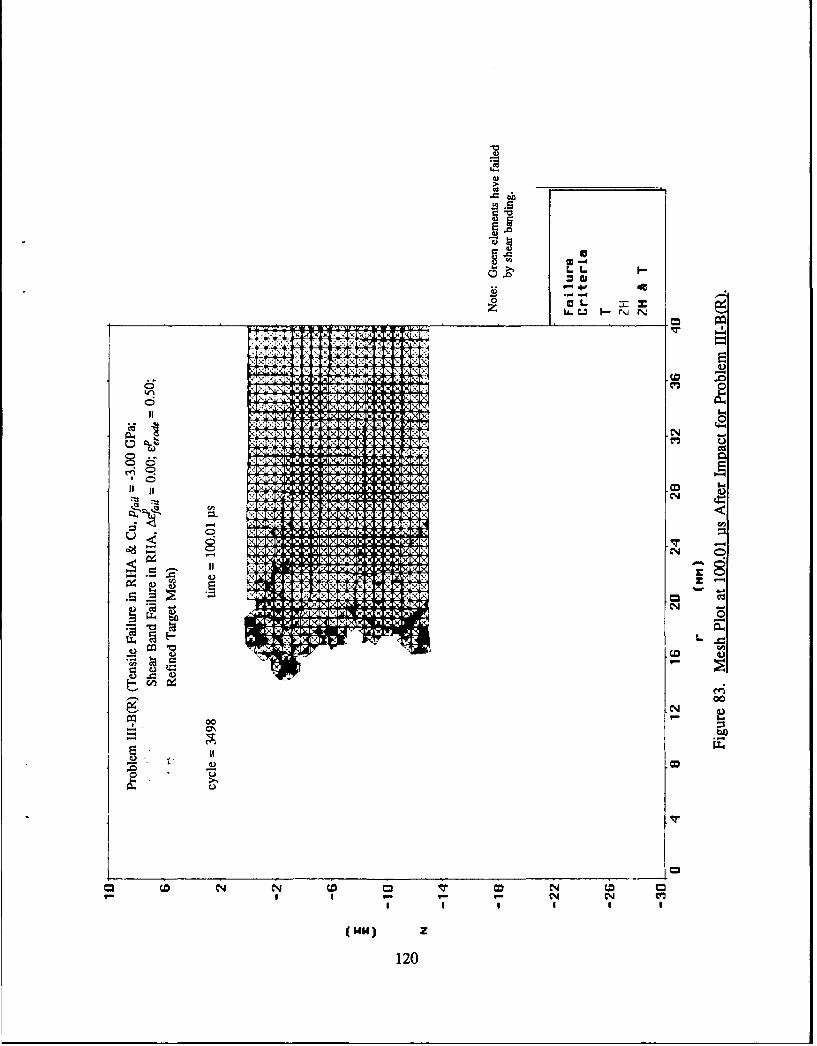
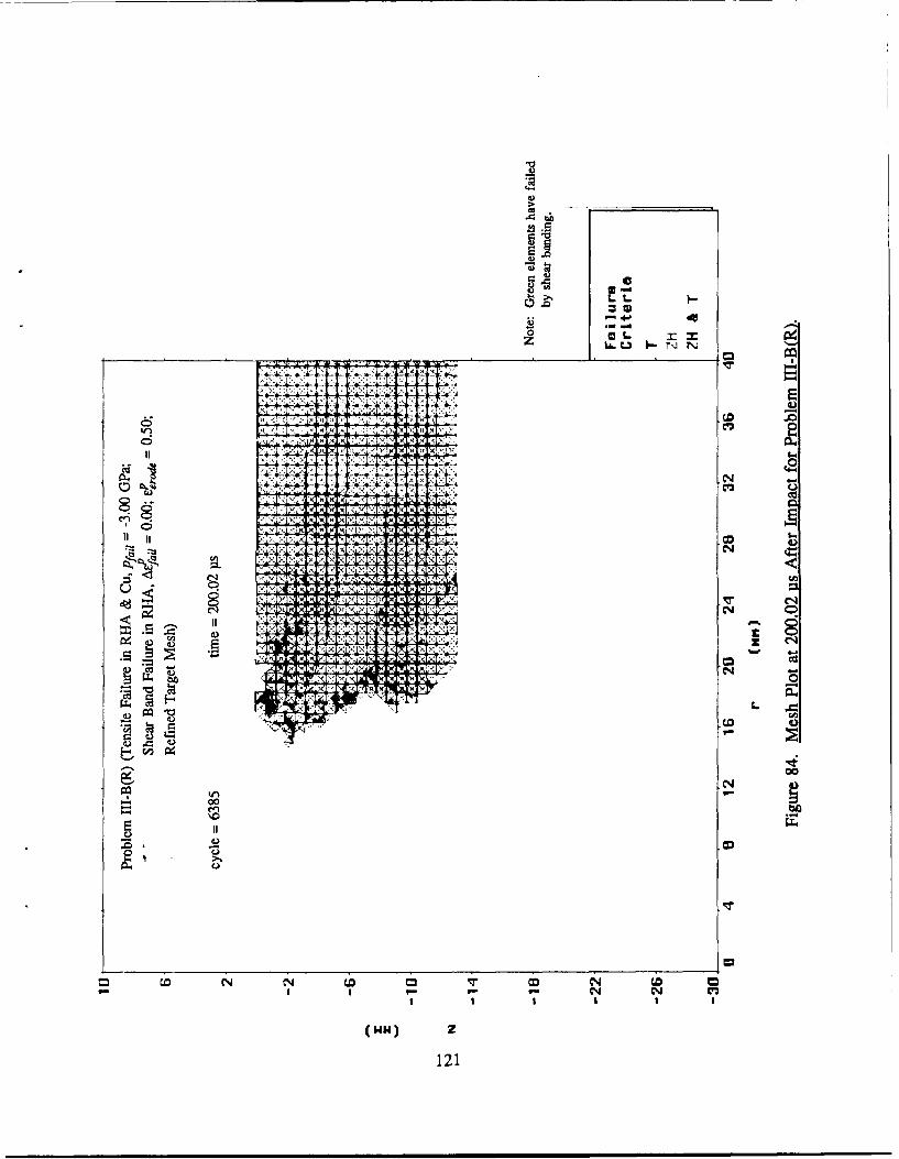
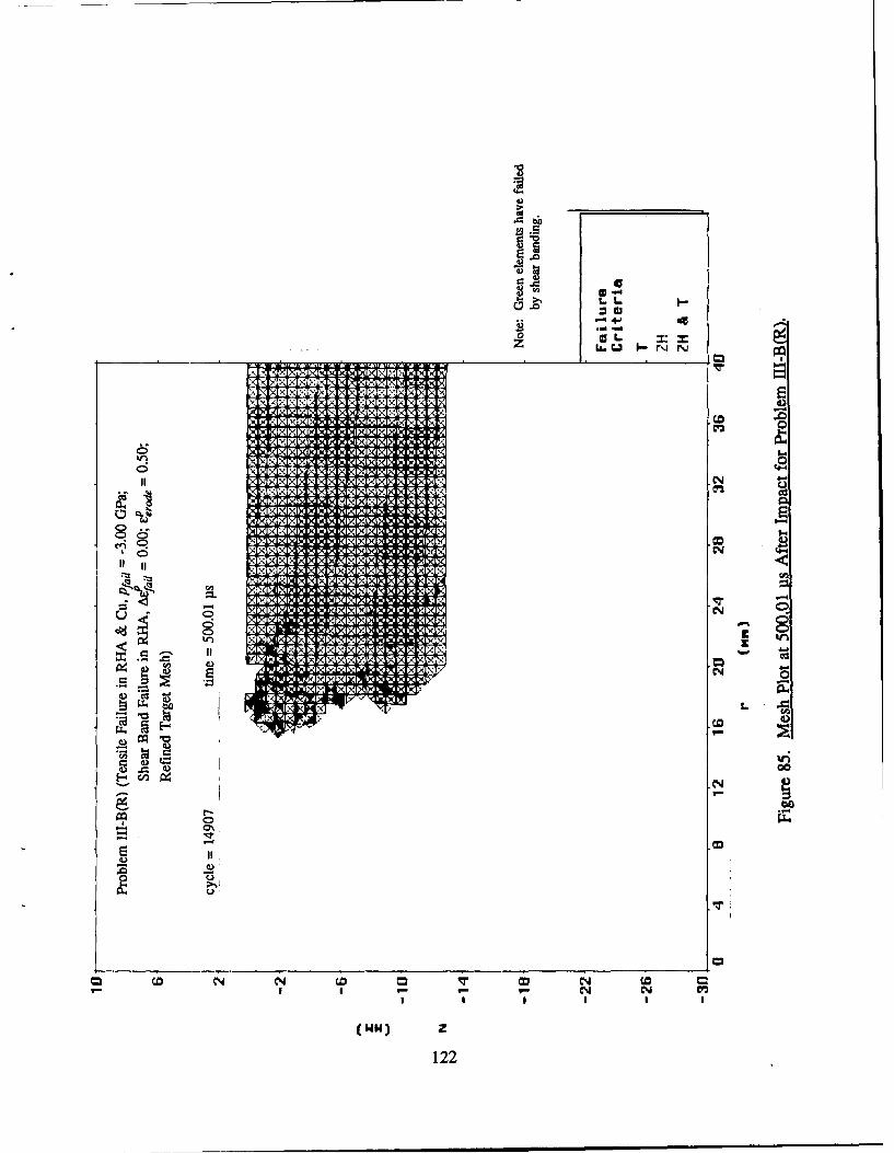
3.01, 4.00, 5.02, 10.02, 20.01, 50.03, 100.01, 200.02 and 500.01 gs after impact in
Figures 75 through 85. These can be compared with Figures 40 through 48, 50 and
54, which pertain to similar times for Problem III-B. Mesh plots at times prior to
perforation are in good qualitative agreement. Spallation in the target plate is again
observed at 3 ts for both meshes. The radial extent of the spall fracture surface is
about 4 mm in Problem III-B(R) and only about 1 mm in Problem III-B. Also, the
spall fracture surface is recessed about 0.8 mm from the exit surface in Problem
III-B(R), while no such recession can be resolved with the coarser mesh of Problem
III-B.
Following perforation, mesh plots from Problem III-B(R) continue to display
good qualitative agreement with those from Problem III-B through 10 pts, both in
terms of the hole boundary's geometry and the general location of zones of elements
that have failed. At 4 and 5 pts, a small zone of elements that have failed in tension
subsequent to failure by shear banding exists at roughly the same location in both
problems. Furthermore, by 10 gts this zone has eroded away in both problems.
By 20 ts after perforation, differences in hole profiles from Problems III-B
and III-B(R) become apparent and seem to be driven by differences in the spatial
distributions of zones of RHA that have failed by shear banding. For example, as
was noted in Section 8, a midsurface-level protuberance remains present in the mesh
at 500 gIs in Problem III-B (Figure 54). This feature is in good agreement with the
experimental hole profile of Figure 11 and shows promise of being preserved in
26
Problem III-B(R) on the basis of the mesh plot at 20 pts (Figure 81). In this figure
a group of RHA elements which have not failed is seen to jut out into a region of
failed elements which line the hole boundary. However, erosion of this group of
unfailed elements occurs between 50 and 100 pts (Figures 82 and 83). This erosion
is assisted by the presence of contiguous failed elements located at about midsurface
elevation and radially outward from the group of unfailed elements in question.
The result is that no prominent midsurface protuberance is present in the final mesh
from Problem III-B(R) (Figure 85). instead, the hole's main throat, or most
narrow cross-section, occurs near the entrance surface, with a lesser throat occurring
near the exit surface. The hole is relatively wide at midsurface elevation. rhoje, the
hole's radius averaged over the plate thickness at 500 pts, is determined for Problem
III-B(R) on the basis of nodal coordinates along the red portion of the target
boundary in Figure 86. The result is 17.3 mm for rhole. This agrees reasonably well
with the experimental result of 18.2 mm, despite the large difference between hole
profile shapes in Figure 85 or 86 and Figure 11. It also agrees reasonably well with
the result of 18.1 mm from Problem III-B. The difference amounts to a 5%
reduction in rhole corresponding to a doubling in mesh fineness.
Next the locations of failed elements in Figure 85 from Problem III-B(R) will
be examined in light of the mesh in Figure 54 from Problem III-B and of
experimental results from Rd. 10771 that were discussed in Section 6. First note
from Figure 85 that no elements that have failed by tensile voids have escaped
slideline erosion by 500 pts. This is inconsistent with the experimental result of
Figure 27, which shows at least nine large, discrete voids distributed around the
midsurface protuberance. Moreover there are no elements that have failed by
tensile voids in the mesh at 50 pts, either among elements in the midsurface that will
shortly erode away or elsewhere (Figure 82). On the other hand the mesh in Figure
85 has retained numerous RHA elements that have failed by shear banding. These
occur mainly in the vicinity of the hole boundary and between the entrance surface
and the midsurface. In contrast Figure 54 shows a more uniform distribution of
predicted shear bands with respect to elevation in the plate. Figure 27 from the
experiment shows two or three shear bands detected near the entrance surface,
consistent with a cluster of failed elements in Figure 85. Most of the shear bands in
Figure 27 lie within the midsurface protuberance. This feature of the experimental
distribution is more consistent with the mesh from Problem III-B(R) at 50 pts than
at 500 g s.
27
Mass lost by the target plate is plotted as a function of time in Figure 87 for
Problems III-B and III-B(R). At all times after 5 gs, the mass loss in Problem
III-B(R) is less than that in Problem III-B. At 500 l.ts, the net mass loss, AM, is
97.2 g in Problem III-B(R) and 105.5 g in Problem III-B (Table 5), corresponding
to an 8.5% difference. This difference of 8.3 g bounds the difference at all earlier
times. The percentage difference between AM from the two problems is larger than
that found above for the quantity rhole. This last comparison is correlated with the
flatter hole profile (i.e., less z dependence of hole radius) at 500 gts for Problem
III-B(R) than for Problem III-B.
t. 9 5 is found from Figure 87 to be 158.3 gis for Problem III-B(R). This
represents a 13.7% decrease from the result of 183.4 gis from Problem III-B (Table
5). These t.95 results from both problems satisfy the experimental bound of
Equation (3).
The results for rhole, AM and t. 95 from Problem III-B(R) are added to Table 6.
Activation of the shear band failure model with the finer mesh has produced some
of the same general effects as in Section 8 with the coarser mesh: The final
perforation hole has grown substantially larger and has been placed in closer
agreement with experiment in terms of size, as witnessed by results for rhole and
AM. Also, the duration of the hole growth process, as measured by t.95, has been
significantly increased over the results obtained with neither failure model or with
only the tensile void model active and has been placed in agreement with the bound
derived from the radiographs of Figure 12. The shape of the final hole profile from
Problem III-B(R) is flatter than both the results from Problem Ill-B and from Rd.
10771. However, variation of the parameters efrode and Aeyail in series of problems
with the finer mesh could presumably have recovered agreement with the
experimental hole shape.
The final issue to consider is the added CPU times associated with the finer
mesh. All calculations described in this report have been performed on the Cray
X-MP/48 computer operated by the U.S. Army Ballistic Research Laboratory. The
CPU times expended in running Problems I-C, I-C(R), II-C, II-C(R), Ill-B and
III-B(R) out to 500 gis are listed in Table 7. CPU times for Problems I-C and 11-C
are very similar, as are those for Problems I-C(R) and II-C(R). Thus for both the
coarser and the finer target mesh, activation of only the tensile void failure model
28
has been accompanied not only by little effect on results for rhole, AM and t. 95 , but
also by little increase in required CPU time. In contrast, for both meshes activation
of the shear band failure model has been accompanied by substantial reduction in
required CPU time. The main reason for this reduction is probably related to the
time step, determined in EPIC-2 by means of the Courant stabililty condition
(Johnson 1976). According to this condition, at any given time in the calculation the
time step is limited by the current dimensions of the smallest non-eroded element.
In problems with the shear band failure model active, more target elements become
eroded and fewer highly distorted elements remain attached to the plate. This
prevents the time step from becoming as small as in the other problems. Doubling
the mesh fineness is seen in Table 7 to have increased the required CPU time by
factors of 7.7, 7.8 and 9.0 in the case of Problems I-C, 11-C and III-B, respectively.
A factor of 8.0 increase was anticipated on the basis of two considerations: (i)
Halving the initial element dimensions very roughly halves the time step throughout
the course of the calculation. (ii) Quadrupling the number of elements very roughly
quadruples the number of operations required at each time step.
The salient results from this section can be briefly summarized as follows: For
each of the three problems run with the finer mesh of Figure 66, the final hole size,
as measured both by rhole and AM, is smaller than the result from the counterpart
problem with the coarser mesh. The differences in terms of rhoIe are 13%, 7% and
5% for Problems I-C(R), II-C(R) and III-B(R), respectively. The differences in
terms of AM for these respective problems are 30%, 18% and 8.5%. rhole and AM
results from Problems I-C, II-C, I-C(R) and II-C(R) are all substantially smaller
than the experimental results, while results for these quantities from Problems III-B
and III-B(R) are all in reasonable agreement with experiment. Specifically, rhole and
AM are respectively 0.5% and 30.% smaller than the experimental results in the case
of Problem III-B and respectively 5% and 40.% smaller in the case of Problem
III-B(R). The final hole shape from Problem III-B is also in reasonable agreement
with experiment, but the final hole profile from Problem III-B(R) is flatter than
according to experiment. The quantity t. 9 5 has been increased in the case of
Problems I-C(R) and II-C(R) by 210.% and 24%, respectively, but decreased by
13.7% in the case of Problem III-B(R) relative to the values obtained with the
coarser mesh. The results for t. 95 from Problems I-C, II-C, I-C(R) and II-C(R) are
smaller than in the experiment, while those from Problems III-B and III-B(R) are
consistent with experiment. Corresponding to the doubling of target mesh fineness,
29
CPU times on a Cray X-MP/48 have increased by factors of 7.7, 7.8 and 9.0 in the
case of Problems I-C, II-C and Ill-B, respectively.
The above-cited quantitative differences between results for rhote, AM and t.95
from Problems III-B and III-B(R) provide measures of the degree to which the
mesh of Figure 15 is adequate for studying parametric dependencies of the solutionupon Perode, Pfail and Aýaiil, as was done in Section 8. This degree of adequacy must
be weighed against the added expense in CPU time associated with performing
parametric studies with the finer mesh of Figure 66. For most researchers, CPU
times given in Table 7 for problems involving the refined mesh are prohibitive for
performing the numerous runs required for parametric studies. A rational basis for
the use of the mesh in Figure 15 is therefore indicated.
10. CONCLUDING REMARKS
This report has discussed the modeling of a particular experiment, in which a
shaped charge warhead was fired at 15.23-charge-diameter standoff into a 13.0-mm-
thick RHA plate. Two quantities evaluated from the experiment and that served as
benchmarks for the calculations are rhole, the final hole radius averaged over the
plate thickness, and AM, the total mass lost by the plate. A third quantity, which
was bounded on the basis of results from two experiments quite similar to Rd.
10771, is t. 95 , the time after impact at which the plate has lost 95% of mass AM.
The experimental results obtained for rhole, AM and 1.95 were 18.2 mm, 136 g, and
the bound t. 95 > 73.9 gts, respectively. A fourth benchmark was provided by a
diagram showing locations of prominent voids and shear bands in a cross-section of
the perforated plate from the original experiment.
A five-parameter geometric model for the leading jet particle was presented.
Its parameters were evaluated on the basis of a radiograph. The particle's length,
volume and centroid location were determined in the process.
Algorithms were developed to simulate material damage associated with the two
micromechanical phenomena of voids and shear bands, both observed in
micrographs of RHA specimens from the perforated plate. Each algorithm, or
failure model, consists of an onset criterion and a post-onset prescription on
stresses. The tensile void failure model, applied to both the OFHC copper of the
30
leading jet particle and the RHA steel of the target plate, introduces the parameter
Pfail for each of the two metals. Pfait is the negative value of pressure which whenreached in an element causes that element to thereafter be restricted from bearing
any deviatoric stress or hydrostatic tension. The shear band failure model, applied
only to the steel, employs as its onset criterion the Zener-Hollomon condition. Thismodel introduces the single parameter ASeaail, the additional equivalent plastic strain
which a failed element can support beyond the level it had attained at the time of
shear banding onset. These algorithms were installed into Lagrangian hydrocode
EPIC-2.
A finite element mesh was developed for the leading jet particle and for the
target plate. That for the target plate consisted of 3200 isosceles right triangles,
each with its longest edge equal to 1.3 mm in length. The contact surface between
the meshes for the leading copper jet particle and the RHA target plate weremodeled by means of the eroding slideline algorithm contained in EPIC-2. This
eroding slideline algorithm introduces the material parameter EPerode, a critical
equivalent plastic strain, for each of OFHC copper and RHA steel. With these
initial meshes fixed, eight series of five problems each were run. In each problemeProde was assigned the same value for both materials.
The first series had neither failure model active for the two metals. The only
parameter varied was ePeroe, over the range of values 0.25, 0.50, 0.75, 1.25 and
2.00. All five problems predicted a plate hole that is smaller and whose formation
is completed earlier than in the experiment. The largest values obtained for rhole,
AM and t. 95 in this series were 13.9 mm, 27.7 g, and 19.4 pts, respectively,
corresponding to respective EProde values of 2.00, 0.75, and 2.00.
The experiment was then remodeled using EPIC-2 with only the tensile void
failure model activated. Throughout this second problem series, parameter Pfail was
assigned the value -3.00 GPa for both RHA and copper. Activation of the tensile
void failure model alone did not significantly increase rhole or AM. Neither was t.95
enlarged significantly, except for the case of P~rode equal to 2.00.
Activation of both the tensile void and the shear band failure models for
Problem Series III through VIII did allow for substantial increases in rhote, AM and
t.95. Pfail was again fixed at -3.00 GPa for both metals. Each of the four problems
31
for which ( e~rode, Aeiail) was assigned the values (0.50, 0.00), (0.75, 0.10), (1.25,
0.25) or (2.00, 0.50) produced an rhole value within 4% of the experimental result.
Of these four problems, the one involving (0.50, 0.00) produced the closest
agreement with experiment in terms of the final hole profile's general shape and the
final location of shear bands within a cross-section of the target plate. None of
these problems predicted a sufficient portion of the plate's final cross-section to be
taken up by voids. These four problems all yielded AM results that were lower than
that of the experiment, by 22%, 18%, 18% and 30%, respectively. Evidently more
highly compressed and bent RHA material remained attached to the plate in the
calculations than in the experiment. On the other hand it was found possible to
produce closer agreement with experiment in terms of AM by tolerating moredeviation in rhole. Thus a fifth problem, for which (eerode, Aefaii) was set to (0.75,
0.00), produced a AM result within 4% of experiment, but an rhole result that was
11% larger than according to experiment. All calculations performed with both
failure models active yielded t.95 results consistent with the experimental bound.
As just described, the tensile void and shear band failure models, when used in
conjunction with the slideline erosion algorithm and a particular mesh for the jet
particle and the target nlate, allowed EPIC-2 to produce reasonable agreement with
a single experiment in terms of final hole geometry, the rate of hole formation, and
the net mass lost by the target plate. Three problems were then rerun with a target
mesh having double the fineness it had in all previous runs. One of these problems
involved no failure modeling, one involved the tensile void failure model only, and
the third involved both the tensile void and the shear band failure models. For the
two problems involving no failure modeling or only tensile failure modeling, no
significant changes in rhole, AM and t. 9 5 were produced by doubling the target mesh
fineness. The final perforation hole remained too small and its formation completed
prematurely in comparison with experiment. The problem with both tensile and
shear banding failure models active that was rerun was the case of Perode and AEimil
equal to 0.50 and 0.00, respectively. This is the case that with the original mesh
gave best overall agreement with experiment in terms of rhole, AM, t,95, the final
hole profile and shear band location within a plate cross-section. Results for this
problem with the refined mesh showed reductions in rhole, AM and t. 9 5 from values
obtained with the original mesh by 5%, 8.5% and 13.7%, respectively. The final
hole profile became flatter (i.e., less elevation dependence in hole radius) than with
the original mesh. The location of shear bands also became less dependent on
32
elevation. For this problem with both failure models active, the CPU time required
on a Cray X-MP/48 demonstrated a factor of 9.0 increase over the time requiredwith the original mesh. In light of this increase, the solution obtained for this
problem with the original was judged to be sufficiently accurate to be useful.
Possibilities for follow-up work will now be considered. In the present study
the criteria of rhole, AM and t.95 agreement with experiment have not uniquely
determined the proper set of input values for the three parameters ,Prode, Pfail andAEcail. In particular, with Pfail fixed at -3.00 GPa for both RHA and copper,agreement was obtained for a range of Perode and Ae8aU combinations. This
consideration motivated the recently conducted set of experiments involving variousconditions of standoff and target plate thickness (Raftenberg 1991, 1992). The same
type of shaped charge warhead used in the two experiments cited in this report was
also employed throughout this newer set of experiments. The question raised is
whether all experiments in this combined database can be reasonably well-matched
in terms of rhole, AM and t.95 by a single set of input values for parameters EProde,
Pfail and Aefail. If satisfactory agreement cannot be obtained or if the threeparameters remain under-determined, some revision of the material models used in
the calculations may be indicated. These would include the models for flow stress,
tensile failure and shear banding failure.
33
Table 1. Parameter Values for the Leading JetParticle's Geometric Model
Parameter Value (mm)Lc 4.77LS 12.75LB 3.08Rs 2.40R 1 3.30
Table 5. Results from Problem Series III Through VIII(Tensile Failure Modeling in RHA & Cu, Pfai = - 3.00 GPa;Shear Band Failure Modeling in RHA, Aefait Varied)
Problem FPerode Ae~ail rhole AM t.95(mm) (g) (Axs)
6 Shear Band Failure in RHA, 1at= 0.00; eP,,,= 0.50;
Refined Target Mesh)
2 cycle = 14907 time = 500.01 ps
-2
-6
-10
N
-14
rhoe= 17.3 nun-18
-22
-26
-30 - I I I I I0 4 a 12 16 20 24 20 32 36 40
r (mn)
NOTE: Thoie calculation based on red portion of boundary.
Figure 86. Mesh Boundary at 500.01 ps and Calculation of rMhoe for Problem III-B(R).
123
ISO
136 g
Problem M-IB
lee ..... ................
0 Problem Mll-(R)
015
0 50 100 190 Z00 250 3900 350 400 450 S00
TIMEi (ps)
Figure 87. Mass Lost From Target Plate vs. Time for Problems III-B and Ifl-B(R).
124
11. REFERENCES
Barbee, Jr., T. W., L. Seaman, R. Crewdson and D. Curran. "Dynamic FractureCriteria for Ductile and Brittle Metals." Journal of Materials, vol. 7, pp. 393-401, 1972.
Johnson, G. R. "Analysis of Elastic-Plastic Impact Involving Severe Distortions."Journal of Applied Mechanics, vol. 98, pp. 439-444, 1976.
Johnson, G. R. and W. H. Cook. "A Constitutive Model and Data for MetalsSubjected to Large Strains, High Strain Rates and High Temperatures."Seventh International Ballistics Symposium Proceedings, The Hague, 1983, pp.541-547.
Johnson, G. R. and W. H. Cook. "Fracture Characteristics of Three MetalsSubjected to Various Strains, High Strain Rates, Temperatures and Pressures."Engineering Fracture Mechanics, vol. 21, pp. 31-48, 1985.
Johnson, G. R. and R. A. Stryk. "User Instructions for the EPIC-2 Code."AFATL-TR-86-51, Air Force Armament Laboratory, Eglin AFB, FL, 1986.
Kohn, B. J. "Compilation of Hugoniot Equations of State." AFWL-TR-69-38, AirForce Weapons Laboratory, Kirtland AFB, NM, 1965.
Raftenberg, M. N. "Experimental Study of RHA Plate Perforation by a Shaped-Charge Jet; Hole Size and Mass Loss." Developments in Mechanics, vol. 16,edited by R. C. Batra and B. F. Armaly, University of Missouri, Rolla, MO, p.34, 1991.
Raftenberg, M. N. "Experimental Investigation of RHA Plate Perforation by aShaped-Charge Jet." Proceedings from the Army Symposium on SolidMechanics, edited by S.-C. Chou, U. S. Army Materials TechnologyLaboratory, Watertown, MA, 1992, in press.
Rinehart, J. S. "Some Quantitative Data Bearing on the Scabbing of Metals underExplosive Attack." Journal of Applied Physics, vol. 22, pp. 555-560, 1951.
Seaman, L., D. R. Curran and D. A. Shockey. "Computational Models for Ductileand Brittle Fracture." Journal of Applied Physics, vol. 47, pp. 4814-4826,1976.
Stecher, F. P. and G. R. Johnson. "Lagrangian Computations for ProjectilePenetration into Thick Plates." Computers in Engineering 1984, vol. 2, editedby W. A. Gruver, A.S.M.E., New York, NY, pp. 292-299, 1984.
U. S. Department of Defense. "Military Specification: Armor Plate, Steel,Wrought, Homogeneous (for Use in Combat-Vehicles and for AmmunitionTesting." MIL-A-12560G(MR), U. S. Army Materials Technology Laboratory,Watertown, MA, 1984.
125
Wright, T.W. and J. W. Walter. "On Stress Collapse in Adiabatic Shear Bands."Journal of the Mechanics and Physics of Solids, vol. 35, pp. 701-720, 1987.
Zener, C. and J. H. J. Hollomon. "Effect of Strain Rate Upon Plastic Flow ofSteel." Journal of Applied Physics, vol. 15, pp. 22-32, 1944.
Zukas, J. A. "Stress Waves in Solids." in Impact Dynamics, edited by J. A. Zukas,T. Nicholas, H. F. Hallock, L. B. Greszcuk and D. R. Curran, Wiley, NewYork, NY, pp. 1-27, 1982.
126
LIST OF SYMBOLS
A, B, C, M, N parameters in the Johnson-Cook strength model
DF, ij component of the plastic part of the rate of deformationtensor
G elastic shear modulus
K 1, K 2 , K 3 parameters in the Mie-Gruneison equation of state
Lc, Ls, LB, Rs, RB parameters in the geometric model for the leading jet particle
Lp length of the leading jet particle
T temperature
Tm melting temperature
Tr room temperature
T* homologous temperature
VP volume of the leading jet particle
e internal energy per underformed volume
f(eP) stress reduction function used in the shear banding failure
model
p pressure
Pfail pressure at which the onset of tensile failure occurs
r radial coordinate
rhole computational hole radius at 500 pts after initial impact,averaged over the target plate's thickness
rho experimental final hole radius averaged over the target plate'sthickness
$iU ij component of the deviatoric Cauchy stress tensor followingreduction
Srr, Szz, See radial, axial, circumferential normal components of thedeviatoric Cauchy stress tensor following reduction
127
Srz shear component of the (deviatoric) Cauchy stress tensorfollowing reduction
s ij component of the deviatoric Cauchy stress tensor prior toreduction
Srr, Szz, soe radial, axial, circumferential normal components of the
deviatoric Cauchy stress tensor prior to reduction
Srz shear component of the (deviatoric) Cauchy stress tensor priorto reduction
t time
t. 95 computational time, after initial impact, at which the targetplate's cumulative mass loss equals 0.95AM
t ".xf. experimental time, after initial impact, at which the targetplate's cumulative mass loss equals 0.95AMeXp"
z axial coordinate
zt, axial coordinate of the centroid of the leading jet particle
AM computational accumulated mass lost by the target plate at 500
ps after initial impact
AMexP experimental total mass lost by the target plate
Aeyii the minimum increment above Eonset of equivalent plastic straincorresponding to which all components of deviatoric Cauchystress within an element are set to zero
F Gruneison coefficient
X expression involving parameters of the geometric model forthe leading jet particle
FP equivalent plastic strain
£erode equivalent plastic strain at which a slideline's master surfaceelement is eroded
£onset equivalent plastic strain within an element at the time of theonset of its failure by shear banding
128
ýP time rate of change of equivalent plastic strain
P fractional change in density from the undeformed state
p density
Po undeformed density
oG equivalent Cauchy stress
CFy flow stress
Grr, (Fz., Cr00 radial, axial, circumferential normal components of the Cauchy
stress tensor
129
INTENTIONALLY LEFT BLANK.
130
No. of No. ofCopies Organization Copies Organization
2 Administrator 1 CommanderDefense Technical Info Center U.S. Army Tank-Automotive CommandATTIN: DIIC-DDA ATTN: ASQNC-TAC-DIT (TechnicalCameron Station Information Center)Alexandria, VA 22304-6145 Warren, MI 48397-5000
Commander 1 DirectorU.S. Army Materiel Command U.S. Army TRADOC Analysis CommandATTN: AMCAM ATTN: ATRC-WSR5001 Eisenhower Ave. White Sands Missile Range, NM 88002-5502Alexandria, VA 22333-0001
1 CommandantCommander U.S. Army Field Artillery SchoolU.S. Army Laboratory Command ATTN: ATSF-CSIATTN: AMSLC-DL FL Sill, OK 73503-50002800 Powder Mill Rd.Adelphi, MD 20783-1145 (Co-- Mii) 1 Commandant
U.S. Army Infantry School2 Commander ATTN: ATSH-CD (Security Mgr.)
U.S. Army Armament Research, Fort Benning, GA 31905-5660Development, and Engineering Center
ATTN: SMCAR-IMI-I (umam cm1') 1 CommandantPicatinny Arsenal, NJ 07806-5000 U.S. Army Infantry School
ATTN: ATSH-CD-CSO-OR2 Commander Fort Benning, GA 31905-5660
U.S. Army Armament Research,Development, and Engineering Center 1 WL/MNOI
Development, and Engineering Center AMXSY-MP, H. CohenATTN: SMCAR-CCB-TLWatervliet, NY 12189-4050 1 Cdr, USATECOM
ATMN: AMSTE-TC(Undca. only) I Commander
U.S. Army Rock Island Arsenal 3 Cdr, CRDEC, AMCCOMATIN: SMCRI-TL1 Technical Library ATTN: SMCCR-RSP-ARock Island, IL 61299-5000 SMCCR-MU
SMCCR-MSIDirectorU.S. Army Aviation Research I Dir, VLAMO
and Technology Activity ATTN: AMSLC-VL-DATTN: SAVRT-R (Library)M/S 219-3 10 Dir, USABRLAmes Research Center ATTN: SLCBR-DD-TMoffett Field, CA 94035-1000
CommanderU.S. Army Missile CommandATTN: AMSMI-RD-CS-R (DOC)Redstone Arsenal, AL 35898-5010
131
No. of No. ofCis Organization Copies Organization
2 Director 1 U.S. Naval AcademyDefense Advanced Research Projects Dept. of Mathematics
Agency ATTN: R. Malek-MadaniATTN: J. Richardson Annapolis, MD 21402
Technical Information1400 Wilson Blvd. 2 Naval Weapons CenterArlington, VA 22209-2308 A'TTN: S. A. Finnegan
Technical Library3 U.S. Army Research Office China Lake, CA 93555
ATTN: J. ChandraK. Iyer 3 Air Force Armament LaboratoryTechnical Library ATrN: J. Foster
P.O. Box 12211 W. Cook4300 Miami Blvd. Technical LibraryResearch Triangle Park, NC 27709 Eglin AFB, FL 32542-5438
U.S. Army MICOM 1 Air Force Wright Aeronautical LaboratoriesATTN: AMSMI-RD-ST-WF, Air Force Systems Command Materials
Michael Schexnayder LaboratoryRedstone Arsenal, AL 35898-5250 ATTN: T. Nicholas
Wright-Patterson AFB, OH 454335 U.S. Army Materials Technology Laboratory
ATTN: SLCMT-MRT, 9 DirectorTony Chou Los Alamos National LaboratoryCharles S. White ATTN: G.E. Co, F663A.M. Rajendran Thomas F. Adams, F663J. Beatty Robert Karpp, MS J960Technical Library John Bolstad, MS G787
Watertown, MA 02172-0001 K. S. Holian, MS B295J. Chapyak
Commander P. FollansbeeU.S. Army Armament Research, G. T. Gray
Development, and Engineering Center Technical LibraryATTN: SMCAR-AA, J. Pearson P.O. Box 1663Picatinny Arsenal, Ni 07806-5000 Los Alamos, NM 87545
2 Commander 1 Sandia National LaboratoriesNaval Surface Warfare Center ATTN: D. BammannATTN: W. Holt Livermore, CA 94550
Technical LibraryDahlgren, VA 22448-5000 1 University of Missouri-Rolla
Dept. of Mechanical and4 Commander Aerospace Engineering
Naval Surface Warfare Center ATTN: R. BatraATTN: F. J. Zerilli Rolla, MO 65401-0249
Code U12, H. ChenCode R14, H. MairCode X21 1, Library
Silver Spring, MD 20902-5000
132
No. of No. ofCo2ie Organization Copies Organization
9 Director 3 Brown UniversityLawrence Livermore National Laboratory Division of EngineeringATIN: Barry R. Bowman, L-122 ATTN: R. Clifton
John E. Reaugh, L-290 J. DuffyMichael J. Murphy A. NeedlemanW. H. Gourdin Providence, RI 02912R. WhirleyG. Goudreau 1 Cornell UniversityD. J. Steinberg, L-35 Dept. of Theoretical and Applied MechanicsRobert Tipton, L-35 ATrN: J. JenkinsTechnical Library Ithaca, NY 14850
P.O. Box 808Livermore, CA 94550 1 North Carolina State University
Dept. of Civil Engineering7 Sandia National Laboratories ATTN: Y. Horie
AITN: L. Davison Raleigh, NC 27607W. HerrmanM. Forrestal 1 North Carolina State UniversityJ. M. McGlaun Dept. of Mechanical EngineeringP. Yarrington ATTN: M. ZikryV. Luk Raleigh, NC 27607D. Grady
P.O. Box 5800 2 The Johns Hopkins UniversityAlbuquerque, NM 87185-5800 Dept. of Mechanical Engineering
Latobe HallDenver Research Institute University ATTN: A. Douglas
of Denver K. T. RameshATMN: R. Recht 34th and Charles StreetsP.O. Box 10127 Baltimore, MD 21218Denver, CO 80210
3 University of CaliforniaMassachusetts Institute of Technology at San DiegoDept. of Mechanical Engineering Dept. of Applied Mechanics andATTN: L. Anand Engineering SciencesCambridge, MA 02139 ATTN: S. Nemat-Nasser
M. MeyersCalifornia Research and Techology, Inc. D. J. BensonAT`TN: Mark Majerus La Jolla, CA 92093P.O. Box 2229Princeton, NJ 08543-2229 1 Northwestern University
Dept. of Applied MathematicsRennselaer Polytechnic Institute ATTN: T. BelytschkoDepL of Computer Science Evanston, IL 60201ATI'N: J. FlahertyTroy, NY 12181 1 University of Illinois
Dept. of Theoretical andApplied Mechanics
ATTN: T. ShawkiUrbana, IL 61801
133
No. of No. ofCopies Organization Copies Organization
University of Texas 1 State University of New York at Stony BrookDept. of Engineering Mechanics Applied Mathematics and Statistics DepartmentATTN: J. Oden ATIN: James GlimmAustin, TX 78712 Stony Brook, NY 11794
University of Maryland 1 Aerojet Precision WeaponsDept. of Mechanical Engineering Dept. 5131/T-WATTN: R. Armstrong ATI'N: Joseph CarleoneCollege Park, MD 20742 1100 Hollyvale
Azusa, CA 91702Washington State UniversityDept. of Physics 2 Dyna East CorporationATIN: Y. Gupta ATTN: P.C. ChouPullman, WA 99163 W. Flis
3201 Arch St.Washington State University Philadelphia, PA 19104Dept. of Mechanical and Materials
Engineering 2 Southwest Research InstituteATTN: H. Zbib ATTN: C. AndersonPullman, WA 99164-2920 S. Bodner
P.O. Drawer 28255Arizona State University San Antonio, TX 78228-0255Mechanical and Aerospace EngineeringM/S 6106 1 BattelleATIN: D. Krajcinovic Edgewood OperationsTempe, AZ 85287-6106 ATTN: R. Jameson
2113 Emmorton Park Rd.Michigan Technological University Edgewood, MD 21040Dept. of Mechanical EngineeringATTN: William W. Predebon 2 Alliant Techsystems, Inc.1400 Townsend Dr. ATTN: Gordon R. JohnsonHoughton, MI 49931-1295 Tim Holmquist
MN 48-2700University of Alabama 7225 Northland Dr.ATTN: S. Jones Brooklyn Park, MN 55428210 Hardaway HallBox 870278 1 S-CubedTuscaloosa, AL 35487-0278 ATMN: R. Sedgwick
P.O. Box 1620University of Texas at El Paso La Jolla, CA 92038-1620Dept. of Metallurgical and Materials
Engineering 1 Orlando Technology, Inc.AT-IN: L. E. Murr ATTN: Dan MatuskaEl Paso, TX 79968 P.O. Box 855
Shalimar, FL 32579
134
No. of
Copie Organization
1 Livermore Software Technology Corp.ATI'N: John 0. Hallquist2876 Waverly WayLivermore, CA 94550
2 SRI InternationalATTN: D. Curran
H. Giovanola333 Ravenswood Ave.Menlo Park, CA 94025
135
No. of
Coijes Organization
1 Defense Research SuffieldATTN: Chris WeickertRalston, Alberta, JOJ 2NO RalstonCanada
1 Ernst Mach InstituteATTN: A. J. StilpEckerstrasse 4D-7800 Frieburg i. Br.Germany
1 Royal Armament R&D EstablishmentATTN: Ian CullisFort HalsteadSevenoaks, Kent TN14 7BJEngland
1 Centre d'Etudes de GramatATTN: SOLVE Gerard46500 GramatFrance
1 Materials Research LaboratoriesATTN: R. L. WoodwardP.O. Box 50Ascot ValeVictoria 3032Australia
I Israel Military IndustriesATTIN: E. HirschRamat Hasharon 47100Israel