arX

iv:1

001.

5404

v3 [

cs.C

C]

8 J

un 2

011

Technical Report: Complexity Analysis by

Graph Rewriting Revisited∗Technical Report

Martin Avanzini

Institute of Computer Science

University of Innsbruck, Austria

martin.avanzini@uibk.ac.at

Georg Moser

Institute of Computer Science

University of Innsbruck, Austria

georg.moser@uibk.ac.at

June 21, 2018

Recently, many techniques have been introduced that allow the (automated)classification of the runtime complexity of term rewrite systems (TRSs forshort). In earlier work, the authors have shown that for confluent TRSs,innermost polynomial runtime complexity induces polytime computabilityof the functions defined.

In this paper, we generalise the above result to full rewriting. Followingour previous work, we exploit graph rewriting. We give a new proof of theadequacy of graph rewriting for full rewriting that allows for a precise controlof the resources copied. In sum we completely describe an implementationof rewriting on a Turing machine (TM for short). We show that the runtimecomplexity of the TRS and the runtime complexity of the TM is polynomiallyrelated. Our result strengthens the evidence that the complexity of a rewritesystem is truthfully represented through the length of derivations. Moreoverour result allows the classification of non-deterministic polytime-computationbased on runtime complexity analysis of rewrite systems.

∗This research is supported by FWF (Austrian Science Fund) projects P20133.

1

Contents

1 Introduction 3

2 Preliminaries 4

3 Term Graph Rewriting 5

4 Adequacy of Graph Rewriting for Term Rewriting 8

5 Implementing Term Rewriting Efficiently 14

6 Discussion 23

2

1 Introduction

Recently we see increased interest into studies of the (maximal) derivation length of termrewrite system, compare for example [8, 7, 12, 9, 11]. We are interested in techniques toautomatically classify the complexity of term rewrite systems (TRS for short) and haveintroduced the polynomial path order POP

∗and extensions of it, cf. [1, 2]. POP∗ is a

restriction of the multiset path order [15] and whenever compatibility of a TRS R withPOP

∗ can be shown then the runtime complexity of R is polynomially bounded. Herethe runtime complexity of a TRS measures the maximal number of rewrite steps as afunction in the size of the initial term, where the initial terms are restricted argumentnormalised terms (aka basic terms).

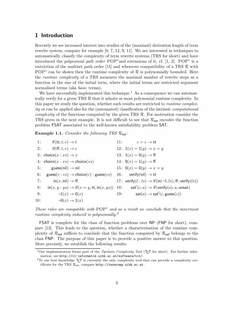
We have successfully implemented this technique.1 As a consequence we can automat-ically verify for a given TRS R that it admits at most polynomial runtime complexity. Inthis paper we study the question, whether such results are restricted to runtime complex-ity or can be applied also for the (automated) classification of the intrinsic computationalcomplexity of the functions computed by the given TRS R. For motivation consider theTRS given in the next example. It is not difficult to see that Rsat encodes the functionproblem FSAT associated to the well-known satisfiability problem SAT.

Example 1.1. Consider the following TRS Rsat:

1: if(tt, t, e)→ t 11: ε = ε→ tt

2: if(ff, t, e)→ e 12: 1(x) = 1(y)→ x = y

3: choice(x : xs)→ x 13: 1(x) = 0(y)→ ff

4: choice(x : xs)→ choice(xs) 14: 0(x) = 1(y)→ ff

5: guess(nil)→ nil 15: 0(x) = 0(y)→ x = y

6: guess(c : cs)→ choice(c) : guess(cs) 16: verify(nil)→ tt

7: in(x, nil)→ ff 17: verify(l : ls)→ if(in(¬l, ls),ff, verify(ls))

8: in(x, y : ys)→ if(x = y, tt, in(x, ys)) 18: sat′(c, a)→ if(verify(a), a, unsat)

9: ¬1(x)→ 0(x) 19: sat(a)→ sat′(c, guess(c))

10: ¬0(x)→ 1(x)

These rules are compatible with POP∗ and as a result we conclude that the innermost

runtime complexity induced is polynomially.2

FSAT is complete for the class of function problems over NP (FNP for short), com-pare [13]. This leads to the question, whether a characterisation of the runtime com-plexity of Rsat suffices to conclude that the function computed by Rsat belongs to theclass FNP. The purpose of this paper is to provide a positive answer to this question.More precisely, we establish the following results:

1Our implementation forms part of the Tyrolean Complexity Tool (TCT for short). For further infor-mation, see http://cl-informatik.uibk.ac.at/software/tct/.

2To our best knowledge TCT is currently the only complexity tool that can provide a complexity cer-tificate for the TRS Rsat, compare http://termcomp.uibk.ac.at.

3

- We re-consider graph rewriting and provide a new proof of the adequacy of graphrewriting for full rewriting. This overcomes obvious inefficiencies of rewriting, whenit comes to the duplication of results.

- We provide a precise analysis of the resources needed in implementing graph rewrit-ing on a Turing machine (TM for short).

- Combining these results we obtain an efficient implementation of rewriting on aTM. Based on this implementation our main result on the correspondence betweenpolynomial runtime complexity and polytime computability follows.

Our result strengthens the evidence that the complexity of a rewrite system is truth-fully represented through the length of derivations. Moreover our result allows the classi-fication of nondeterministic polytime-computation based on runtime complexity analysisof rewrite systems. This extends previous work (see [3]) that shows that for confluentTRSs, innermost polynomial runtime complexity induces polytime computability of thefunctions defined. Moreover it extends related work by Dal Lago and Martini (see [6, 5])that studies the complexity of orthogonal TRSs, also applying graph rewriting tech-niques.

The paper is structured as follows. In Section 2 we present basic notions, in Section 3we (briefly) recall the central concepts of graph rewriting. The adequacy theorem isprovided in Section 4 and in Section 5 we show how rewriting can be implementedefficiently. Finally we discuss our results in Section 6, where the above application tocomputational complexity is made precise.

2 Preliminaries

We assume familiarity with the basics of term rewriting, see [4, 15]. No familiarity withgraph rewriting (see [15]) is assumed. Let R be a binary relation on a set S. We writeR+ for the transitive and R∗ for the transitive and reflexive closure of R. An elementa ∈ S is R-minimal if there exists no b ∈ S such that a R b.

Let V denote a countably infinite set of variables and F a signature, containing atleast one constant. The set of terms over F and V is denoted as T . The size |t| of aterm t is defined as usual. A term rewrite system (TRS for short) R over T is a finiteset of rewrite rules l → r, such that l /∈ V and Var(l) ⊇ Var(r). We write −→R for theinduced rewrite relation. The set of defined function symbols is denoted as D, while theconstructor symbols are collected in C, clearly F = D ∪ C. We use NF(R) to denote theset of normal forms of R and write s −→!

R t if s −→∗R t and t ∈ NF(R). We define the

set of values Val := T (C,V), and we define B := f(v1, . . . , vn) | f ∈ D and vi ∈ Val asthe set of basic terms. Let be a fresh constant. Terms over F ∪ and V are calledcontexts. The empty context is denoted as . For a context C with n holes, we writeC[t1, . . . , tn] for the term obtained by replacing the holes from left to right in C withthe terms t1, . . . , tn.

4

A TRS is called confluent if for all s, t1, t2 ∈ T with s −→∗R t1 and s −→∗

R t2 there existsa term t3 such that t1 −→

∗R t3 and t2 −→

∗R t3. The derivation length of a terminating term

s with respect to→ is defined as dl(s,→) := maxn | ∃t. s→n t, where→n denotes then-fold application of →. The runtime complexity function rcR with respect to a TRS Ris defined as rcR(n) := maxdl(t,−→R) | t ∈ B and |t| 6 n.

3 Term Graph Rewriting

In the sequel we introduce the central concepts of term graph rewriting or graph rewritingfor short. We closely follow the presentation of [3], for further motivation of the presentednotions we kindly refer the reader to [3]. Let R be a TRS over a signature F . We keepR and F fixed for the remainder of this paper.

A graph G = (VG,SuccG,LG) over the set L of labels is a structure such that VG is afinite set, the nodes or vertexes, Succ : VG → V∗

G is a mapping that associates a node uwith an (ordered) sequence of nodes, called the successors of u. Note that the sequenceof successors of u may be empty: SuccG(u) = []. Finally LG : VG → L is a mapping thatassociates each node u with its label LG(u). Typically the set of labels L is clear fromcontext and not explicitly mentioned. In the following, nodes are denoted by u, v, . . .possibly followed by subscripts. We drop the reference to the graph G from VG, SuccG,and LG, i.e., we write G = (V,Succ,L) if no confusion can arise from this. Further, wealso write u ∈ G instead of u ∈ V.

Let G = (V,Succ,L) be a graph and let u ∈ G. Consider Succ(u) = [u1, . . . , uk]. We

call ui (1 6 i 6 k) the i-th successor of u (denoted as ui ui). If u

i v for some i, then

we simply write u v. A node v is called reachable from u if u∗ v, where

∗ denotes

the reflexive and transitive closure of . We write+ for ·

∗. A graph G is acyclic

if u+ v implies u 6= v and G is rooted if there exists a unique node u such that every

other node in G is reachable from u. The node u is called the root rt(G) of G. The sizeof G, i.e., the number of nodes, is denoted as |G|. The depth of S, i.e., the length of thelongest path in S, is denoted as dp(S). We write Gu for the subgraph of G reachablefrom u.

Let G and H be two term graphs, possibly sharing nodes. We say that G and H areproperly sharing if u ∈ G ∩H implies LG(u) = LH(u) and SuccG(u) = SuccH(u). If Gand H are properly sharing, we write G ∪H for their union.

Definition 3.1. A term graph (with respect to F and V) is an acyclic and rooted graphS = (V,Succ,L) over labels F ∪ V. Let u ∈ S and suppose L(u) = f ∈ F such that f isk-ary. Then Succ(u) = [u1, . . . , uk]. On the other hand, if L(u) ∈ V then Succ(u) = [].We demand that any variable node is shared. That is, for u ∈ S with L(u) ∈ V, ifL(u) = L(v) for some v ∈ V then u = v.

Below S, T, . . . and L,R, possibly followed by subscripts, always denote term graphs.We write Graph for the set of all term graphs with respect to F and V. Abusing notationfrom rewriting we set Var(S) := u | u ∈ S,L(u) ∈ V, the set of variable nodes in S.We define the term term(S) represented by S as follows: term(S) := x if L(rt(S)) =

5

x ∈ V and term(S) := f(term(S u1), . . . , term(S uk)) for L(rt(S)) = f ∈ F andSucc(rt(S)) = [u1, . . . , uk].

We adapt the notion of positions in terms to positions in graphs in the obvious way.Positions are denoted as p, q, . . . , possibly followed by subscripts. For positions p andq we write pq for their concatenation. We write p 6 q if p is a prefix of q, i.e., q = pp′

for some position p′. The size |p| of position p is defined as its length. Let u ∈ S bea node. The set of positions PosS(u) of u is defined as PosS(u) := ε if u = rt(S)

and PosS(u) := i1 · · · ik | rt(S)i1 · · ·

ik u otherwise. The set of all positions in S isPosS :=

⋃

u∈S PosS(u). Note that PosS coincides with the set of positions of term(S).If p ∈ PosS(u) we say that u corresponds to p. In this case we also write S p for thesubgraph S u. This is well defined since exactly one node corresponds to a position p.One verifies term(S p) = term(S)|p for all p ∈ PosS . We say that u is (strictly) abovea position p if u corresponds to a position q with q 6 p (q < p). Conversely, the node uis below p if u corresponds to q with p 6 q.

By exploiting different degrees of sharing, a term t can often be represented by morethan one term graph. Let S be a term graph and let u ∈ S be a node. We say thatu is shared if the set of positions PosS(u) is not singleton. Note that in this case, thenode u represents more than one subterm of term(S). If PosS(u) is singleton, thenu is unshared. The node u is minimally shared if it is a variable node or unsharedotherwise (recall that variable nodes are always shared). We say u is maximally sharedif term(S u) = term(S v) implies u = v. The term graph S is called minimally sharing(maximally sharing) if all nodes u ∈ S are minimally shared (maximally shared). Let sbe a term. We collect all minimally sharing term graphs representing s in the set (s).Maximally sharing term graphs representing s are collected in (s).

We now introduce a notion for replacing a subgraph S u of S by a graph H.

Definition 3.2. Let S be a term graph and let u, v ∈ S be two nodes. Then S[u←− v]denotes the redirection of node u to v: set r(u) := v and r(w) := w for all w ∈ S \ u.Set V′ := (VS ∪v) \ u and for all w ∈ V′, Succ′(w) := r∗(SuccS(w)) where r∗ is theextension of r to sequences. Finally, set S[u←− v] := (V′,Succ′,LS).

Let H be a rooted graph over F∪V. We define S[H]u := (S[u←− rt(H)] ∪H)v wherev = rt(H) if u = rt(S) and v = rt(S) otherwise. Note that S[H]u is again a term graphif u 6∈ H and H acyclic.

The following notion of term graph morphism plays the role of substitutions.

Definition 3.3. Let L and T be two term graphs. A morphism from L to T (denotedm : L → T ) is a function m : VL → VT such that m(rt(L)) = rt(T ), and for all u ∈ Lwith LL(u) ∈ F , (i) LL(u) = LT (m(u)) and (ii) m∗(SuccL(u)) = SuccT (m(u)).

The next lemma follows essentially from assertion (ii) of Definition 3.3.

Lemma 3.4. If m : L→ S then for any u ∈ S we have m : Lu→ S m(u).

Proof. By a straight forward inductive argument.

6

Letm : L→ S be a morphism from L to S. The induced substitution σm : Var(L)→ Tis defined as σm(x) := term(S m(u)) for any u ∈ S such that L(u) = x ∈ V. As an easyconsequence of Lemma 3.4 we obtain the following.

Lemma 3.5. Let L and S be term graphs, and suppose m : L→ S for some morphismm. Let σm be the substitution induced by m. Then term(L)σm = term(S).

Proof. The lemma has also been shown in [3, Lemma 14]. For completeness we restatethe proof.

We prove that for each node u ∈ L, term(L u)σm = term(S m(u)) by inductionon l := term(L u). To conclude term(L)σm = term(S), it suffices to observe that bydefinition of m: m(rt(L)) = rt(S).

If l ∈ V, then by definition Lu consists of a single (variable-)node and lσm = term(S

m(u)) follows by the definition of the induced substitution σm. If l = f(l1, . . . , lk),then we have SuccL(u) = [u1, . . . , uk] for some u1, . . . , uk ∈ L. As m : L → S holds,Lemma 3.4 yields m : L ui → S m(ui) for all i = 1, . . . , k. And induction hypothesisbecomes applicable so that liσm = term(S m(ui)). Thus

lσm = f(l1σm, . . . , lkσm) = f(term(S m(u1)), . . . , term(S m(uk))) .

By definition of m, LS(m(u)) = LL(u) = f and SuccS(m(u)) = m∗(SuccL(u)) =[m(u1), . . . ,m(uk)]. Hence f(term(S m(u1)), . . . , term(S m(uk))) = term(S m(u)).

We write S >m T (or S > T for short) if m : S → T is a morphism such that for allu ∈ VS , Property (i) and Property (ii) in Definition 3.3 are fulfilled. For this case, Sand T represent the same term. We write S >m T (or S > T for short) when the graphmorphism m is additionally non-injective. If both S > T and T > S holds then S andT are isomorphic, in notation S ∼= T . Recall that |S| denotes the number of nodes in S.

Lemma 3.6. For all term graph S and T , S >m T implies term(S) = term(T ) and|S| > |T |. If further S >m T holds then |S| > |T |.

Proof. Suppose S >m T We first prove term(S) = term(T ). We prove the lemma byinduction on S. For the base case, suppose S consists of a single node u such thatLS(u) = x ∈ V. As the node u is the root of S, definition of m yields that T consistsof a single (variable)-node labeled with x. (Note that m is a surjective morphism.)Thus the result follows trivially. For the inductive step, suppose LS = f ∈ F andSuccS = [u1, . . . , uk]. From S >m T we see that LT = f and SuccT = [m(u1), . . . ,m(uk)].As a consequence of Lemma 3.4, S ui >m T m(ui) and thus by induction hypothesisterm(S ui) = term(T m(ui)) as desired.

Now observe that m is by definition surjective. Thus |S| > |T | trivially follows.Further, it is not hard to see that if m is additionally non-injective, i.e., S >m T , thenclearly |S| > |T |.

Let L and R be two properly sharing term graphs. Suppose rt(L) 6∈ Var(L), Var(R) ⊆Var(L) and rt(L) 6∈ R. Then the graph L ∪ R is called a graph rewrite rule (rule for

7

short), denoted by L → R. The graph L, R denotes the left-hand, right-hand side ofL→ R respectively. A graph rewrite system (GRS for short) G is a set of graph rewriterules.

Let G be a GRS, let S ∈ Graph and let L → R be a rule. A rule L′ → R′ is called arenaming of L → R with respect to S if (L′ → R′) ∼= (L → R) and VS ∩VL′→R′ = ∅.Let L′ → R′ be a renaming of a rule (L → R) ∈ G for S, and let u ∈ S be a node.We say S rewrites to T at redex u with rule L → R, denoted as S −→G,u,L→R T , ifthere exists a morphism m : L′ → S u and T = S[m(R′)]u. Here m(R′) denotes thestructure obtained by replacing in R′ every node v ∈ dom(m) by m(v) ∈ S, where thelabels of m(v) ∈ m(R′) are the labels of m(v) ∈ S. We also write S −→G,p,L→R Tif S −→G,u,L→R T for the position p corresponding to u in S. We set S −→G T ifS −→G,u,L→R T for some u ∈ S and (L→ R) ∈ G. The relation −→G is called the graphrewrite relation induced by G. Again abusing notation, we denote the set of normal-formswith respect to −→G as NF(G).

4 Adequacy of Graph Rewriting for Term Rewriting

In earlier work [3] we have shown that graph rewriting is adequate for innermost rewritingwithout further restrictions on the studied TRS R. In this section we generalise thisresult to full rewriting. The here presented adequacy theorem (see Theorem 4.15) isnot essentially new. Related results can be found in the extensive literature, see forexample [15]. In particular, in [14] the adequacy theorem is stated for full rewriting andunrestricted TRSs. In this work, we take a fresh look from a complexity related pointof view. We give a new proof of the adequacy of graph rewriting for full rewriting thatallows for a precise control of the resources copied. This is essential for the accuratecharacterisation of the implementation of graph rewriting given in Section 5.

Definition 4.1. The simulating graph rewrite system G(R) of R contains for each rule(l → r) ∈ R some rule L→ R such that L ∈ (l), R ∈ (r) and VL ∩VR = Var(R).

The next two Lemmas establish soundness in the sense that derivations with respectto G(R) correspond to R-derivations.

Lemma 4.2. Let S be a term graph and let L → R be renaming of a graph rewriterule for S, i.e., S ∩ R = ∅. Suppose m : L → S for some morphism m and let σm bethe substitution induced by m. Then term(R)σm = term(T ) where T := (m(R) ∪ S) rt(m(R)).

Proof. We prove the more general statement that for each u ∈ R, term(R u)σm =term(T m(u)), c.f. also [3, Lemma 15]. First suppose u ∈ R ∩ L. Then R u = L uas L, R are properly shared. Employing Lemma 3.5, we have term(Ru)σm = term(L

u)σm = term(S m(u)). From this the assertion follows.Thus suppose u ∈ R \ L. This subcase we prove by induction on r := term(R u).

The base case r ∈ V is trivial, as variables are shared in L→ R. For the inductive step,let r = f(r1, . . . , rk) with SuccR(u) = [u1, . . . , uk]. We identify m with the extension

8

of m to all nodes in R. The induction hypothesis yields riσm = term(T m(ui)) fori = 1, . . . , k. By definition of m(R): m(u) = u ∈ m(R) ⊆ T . Hence SuccT (m(u)) =Succm(R)(u) = m∗(SuccR(u)) = [m(u1), . . . ,m(uk)]. Moreover LT (u) = Lm(R)(u) = fby definition. We conclude rσm = f(r1σm, . . . , rkσm) = f(term(T m(u1)), . . . , term(T

m(uk))) = term(T m(u)).

In Section 2 we introduced as designation of the empty context. Below we write

for the unique (up-to isomorphism) graph representing the constant .

Lemma 4.3. Let S and T be two be properly sharing term graphs, let u ∈ S \ T andC = term(S[]u). Then term(S[T ]u) = C[term(T ), . . . , term(T )].

Proof. We proceed by induction on the size of S, compare also [3, Lemma 16]. In thebase case S consists of a single node u. Hence the context C is empty and the lemmafollows trivially.

For the induction step we can assume without loss of generality that u 6= rt(S). Weassume LS(rt(S)) = f ∈ F and SuccS(rt(S)) = [v1, . . . , vk]. For all i (1 6 i 6 k) suchthat vi = u set Ci = and for all i such that vi 6= u but (S[T ]u) vi = (S vi)[T ]u weset Ci = term((S vi)[]u). In the latter sub-case induction hypothesis is applicable toconclude

term((

S[T ]u)

vi)

= Ci[term(T ), . . . , term(T )] .

Finally we set C := f(C1, . . . , Ck) and obtain C = term(S[]u). In sum we haveterm(S[T ]u) = f

((

S[T ]u)

v1, . . . ,(

S[T ]u)

vk)

= C[term(T )], where term(T ) denotesthe sequences of terms term(T ).

For non-left-linear TRSs R, −→G(R) does not suffice to mimic −→R. This is clarifiedin the following example.

Example 4.4. Consider the TRS Rf := f(x)→ eq(x, a); eq(x, x)→ ⊤. Then Rf

admits the derivationf(a) −→Rf

eq(a, a) −→Rf⊤

but G(Rf) cannot completely simulate the above sequence:

f

a

eq

a a

−→G(Rf ) ∈ NF(G(Rf))

Let L → R be the rule in G(Rf) corresponding to eq(x, x) → ⊤, and let S, term(S) =eq(a, a), be the second graph in the above sequence. Then L → R is inapplicable as wecannot simultaneously map the unique variable node in L to both leaves in S via a graphmorphism. Note that the situation can be repaired by sharing the two arguments in S.

For maximally sharing graphs S we can prove that redexes of R and (positions corre-sponding to) redexes of G(R) coincide. This is a consequence of the following Lemma.

9

Lemma 4.5. Let l be a term and s = lσ for some substitution σ. If L ∈ (l) andS ∈ (s), then there exists a morphism m : L → S. Further, σ(x) = σm(x) for theinduces substitution σm and all variables x ∈ Var(l).

Proof. We prove the lemma by induction on l. It suffices to consider the induction step.Let l = f(l1, . . . , lk) and s = f(l1σ, . . . , lkσ). Suppose SuccL(rt(L)) = [u1, . . . , uk] andSuccS(rt(S)) = [v1, . . . , vk]. By induction hypothesis there exist morphisms mi : L

ui → S vi (1 6 i 6 k) of the required form. Define m : VL → VS as follows. Setm(rt(L)) = rt(S) and for w 6= rt(L) define m(w) = mi(w) if w ∈ dom(mi). Weclaim w ∈ (dom(mi) ∩ dom(mj)) implies mi(w) = mj(w). For this, suppose w ∈(dom(mi) ∩ dom(mj)). Since L ∈ (l), only variable nodes are shared, hence w needsto be a variable node, say LL(w) = x ∈ V. Then

term(S mi(w)) = σmi(x) = σ(x) = σmj

(x) = term(S mj(w))

by induction hypothesis. As S ∈ (s) is maximally shared, mi(w) = mj(w) follows. Weconclude m is a well-defined morphism, further m : L→ S.

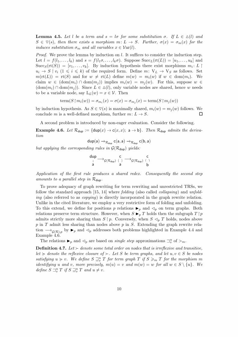
A second problem is introduced by non-eager evaluation. Consider the following.

Example 4.6. Let Rdup := dup(x)→ c(x, x); a→ b. Then Rdup admits the deriva-tion

dup(a) −→Rdupc(a, a) −→Rdup

c(b, a)

but applying the corresponding rules in G(Rdup) yields:

dup

a

c

a

c

b

−→G(Rdup)−→G(Rdup)

Application of the first rule produces a shared redex. Consequently the second stepamounts to a parallel step in Rdup.

To prove adequacy of graph rewriting for term rewriting and unrestricted TRSs, wefollow the standard approach [15, 14] where folding (also called collapsing) and unfold-ing (also referred to as copying) is directly incorporated in the graph rewrite relation.Unlike in the cited literature, we employ a very restrictive form of folding and unfolding.To this extend, we define for positions p relations p and ⊳p on term graphs. Bothrelations preserve term structure. However, when S p T holds then the subgraph T padmits strictly more sharing than S p. Conversely, when S ⊳p T holds, nodes abovep in T admit less sharing than nodes above p in S. Extending the graph rewrite rela-tion −→G(R),p by p and ⊳p addresses both problems highlighted in Example 4.4 andExample 4.6.

The relations p and ⊳p are based on single step approximations ⊐uv of >m.

Definition 4.7. Let ≻ denote some total order on nodes that is irreflexive and transitive,let < denote the reflexive closure of ≻. Let S be term graphs, and let u, v ∈ S be nodessatisfying u < v. We define S ⊒u

v T for term graph T if S >m T for the morphism midentifying u and v, more precisely, m(u) = v and m(w) = w for all w ∈ S \ u. Wedefine S ⊐u

v T if S ⊒uv T and u 6= v.

10

We write S ⊒v T (S ⊐v T ) if there exists u ∈ S such that S ⊒uv T (S ⊐u

v T ) holds.Similar S ⊒ T (S ⊐ T ) if there exist nodes u, v ∈ S such that S ⊒u

v T (S ⊐uv T ) holds.

Example 4.8. Consider the term t = (0 + 0) × (0 + 0). Then t is represented by thefollowing three graphs that are related by ⊏2

3and ⊐

4

5 respectively.

➀×

➂+

➃ 0 ➄ 0

T1

⊏2

3

➀×

➁+ ➂+

➃ 0 ➄ 0

T2

⊐4

5

➀×

➁+ ➂+

➄ 0

T3

Put otherwise, the term graph T2 is obtained from T1 by copying node 3, introducing thefresh node 2. The graph T3 is obtained from T2 by collapsing node 4 onto node 5.

Suppose S ⊐uv T . Then the morphism underlying ⊐u

v defines the identity on VS \u.In particular, it defines the identity on successors of u, v ∈ S. Thus the following isimmediate.

Lemma 4.9. Let S be a term graph, and let u, v ∈ S be two distinct nodes. Then thereexists a term graph T such that S ⊐u

v T if and only if LS(u) = LS(v) and SuccS(u) =SuccS(v).

Proof. We prove the direction from left to right as the other is trivial. Suppose S ⊐uv T

and let m be the morphism underlying ⊐uv . Observe m(u) = m(v) = v. And thus

LS(u) = LT (m(u)) = LT (v) = LT (m(v)) = LS(v) follows. To prove the second assertion,

pick nodes ui and vi such that ui ui and v

i vi. Since S >m T we obtain m(ui) =

m(vi). Thus ui 6= vi if and only if either ui = u or vi = u. The former implies that Sis cyclic, the latter implies that T is cyclic, contradicting that S is a term graph or m amorphism. We conclude ui = vi for i arbitrary, hence SuccS(u) = SuccS(v).

The restriction u < v was put onto ⊒uv so that ⊒v enjoys the following diamond

property. Otherwise, the peak ⊏uv · ⊐

vu ⊆∼= cannot be joined.

Lemma 4.10. ⊑u · ⊒v ⊆ ⊒w1· ⊑w2

where w1, w2 ∈ u, v.

Proof. Assume T1 ⊑u′

u S ⊒v′

v T2 for some term graphs S, T1 and T2. The only non-trivial case is T1 ⊏u′

u S ⊐v′

v T2 for u′ 6= v′ and u 6= v. We prove T1 ⊐w1· ⊏w2

T2 forw1, w2 ∈ u, v by case analysis.

- Case T1 ⊏u′

w S ⊐v′

w T2 for v′ 6= u′. We claim T1 ⊐v′

w · ⊏u′

w T2. Let m1 bethe morphism underlying ⊏u′

w and let m2 be the morphism underlying ⊐v′

w (c.f.Definition 4.7). We first show LT1(v

′) = LT1(w) and SuccT1(v′) = SuccT1(w).

Using Lemma 4.9, S ⊐v′

w T2 yields LS(v′) = LS(w). Employing v′ 6= u′ and w 6= u′

we see

LT1(v′) = LT1(m1(v

′)) = LS(v′) = LS(w) = LT1(m1(w)) = LT1(w)

11

where we employ m1(v′) = v′ and m1(w) = w. Again by Lemma 4.9, we see

SuccS(u′) = SuccS(w) and SuccS(v

′) = SuccS(w) by the assumption T1 ⊏u′

w S ⊐v′

w

T2. We conclude SuccS(v′) = SuccS(w) and thus

SuccT1(v′) = SuccT1(m1(v

′)) = m∗1(SuccS(v

′))= m∗

1(SuccS(w)) = SuccT1(m1(w)) = SuccT1(w) .

By Lemma 4.9 we see T1 ⊐v′

w U1 for some term graph U1. Symmetrically, we canprove T2 ⊐u′

w U2 for some term graph U2. Hence T1 ⊐v′

w · ⊏u′

w T2 holds if U1 = U2.To prove the latter, one showsm2 ·m1 = m1 ·m2 by a straight forward case analysis.

- Case T1 ⊏wu S ⊐w

v T2 for u 6= v. Without loss of generality assume u ≻ v.We claim T1 ⊐u

v · ⊏uv T2 and follow the pattern of the proof for the previous

case. Note that LT1(u) = LT1(v) follows from LS(u) = LS(w) = LS(v) as before,similar SuccT1(u) = SuccT1(v) follows from SuccS(u) = SuccS(w) = SuccS(v) withw 6∈ SuccS(w). Hence T1 ⊐

uv U1 and symmetrically T2 ⊐

uv U2 for some term graphs

U1 and U2. One verifies m ·m1 = m ·m2 for graph morphisms m1 underlying ⊐wu ,

m2 underlying ⊐wv , and m underlying ⊐u

v . We conclude T1 ⊐uv · ⊏

uv T2.

- Case T1 ⊏wu S ⊐v′

w T2. Note v′ ≻ u since v′ ≻ w ≻ u by the assumption. Weclaim T1 ⊐v′

u · ⊏wu T2. From the assumption we obtain LS(u) = LS(w) = LS(v

′)and SuccS(u) = SuccS(w) = SuccS(v

′), from which we infer LT1(v′) = LT1(u) and

SuccT1(v′) = SuccT1(u) (employing w 6∈ SuccS(w)). Further, LT2(w) = LT2(u) and

SuccT2(w) = SuccT2(u) (employing v′ 6∈ SuccS(v′)). We conclude T1 ⊐v′

u U1 andsimilar T2 ⊐

wu U2. Finally, one verifies U1 = U2 by case analysis.

- Case T1 ⊏u′

u S ⊐v′

v T2 for pairwise distinct u′, u, v′ and v. We show T1 ⊐

v′

v · ⊏u′

u T2.Let m be the morphism underlying ⊐u′

u . Observe m(v) = v and m(v′) = v′

by our assumption. Hence LT1(v′) = LS(v

′) = LS(v) = LT1(v) and LT1(v′) =

m∗(LS(v′)) = m∗(LS(v)) = LT1(v). We obtain T1 ⊐v′

v U1 and symmetricallyT2 ⊐u′

u U2 for some term graphs U1 and U2. Finally, one verifies U1 = U2 by caseanalysis as above.

The above lemma implies confluence of ⊒. Since ⊐∗ = ⊒∗, also ⊐ is confluent.

Definition 4.11. Let S be a term graph and let p be a position in S. We say that Sfolds strictly below p to the term graph T , in notation S p T , if S ⊐u

v T for nodesu, v ∈ S strictly below p in S. The graph S unfolds above p to the term graph T , innotation S ⊳p T , if S ⊏u

v T for some unshared node u ∈ T above p, i.e., PosT (u) = qfor q 6 p.

Example 4.12. Reconsider the term graphs T1, T2 and T3 with T1 ⊏2

3T2 ⊐

4

5 T3 fromExample 4.8. Then T1 ⊳2 T2 since node 3 is an unshared node above position 2 in T2.Further T2 2 T3 since both nodes 4 and 5 are strictly below position 2 in T2.

12

Note that for S ⊐uv T the sets of positions PosS and PosT coincide, thus the n-fold

composition ⊳np of ⊳p (and the n-fold composition n

p of p) is well-defined for p ∈ PosS .In the next two lemmas we prove that relations ⊳p and p fulfill their intended purpose.

Lemma 4.13. Let S be a term graph and p a position in S. If S is ⊳p-minimal thenthe node corresponding to p is unshared.

Proof. By way of contradiction, suppose S is ⊳p-minimal but the node w correspondingto p is shared. We construct T such that S ⊳p T . We pick an unshared node v ∈ S,and shared node vi ∈ S, above p such that v vi. By a straight forward induction onp we see that v and vi exist as w is shared. For this, note that at least the root of S isunshared.

Define T := (VT ,LT ,SuccT ) as follows: let u be a fresh node such that uSucc vi. setVT := VS ∪u; set LT (u) := LS(vi) and SuccT (u) := SuccS(vi); further replace the edge

vi vi by v

i u, that is, set LT (v) := [v1, . . . , u, . . . , vl] for LS(v) = [v1, . . . , vi, . . . , vl].

For the remaining cases, define LT (w) := LS(u) and SuccT (w) := SuccS(w). One easilyverifies T ⊐u

viS. Since by way of construction u is an unshared node above p, S ⊳p T

holds.

Lemma 4.14. Let S be a term graph, let p be a position in S. If S is p-minimal thenthe subgraph S p is maximally shared.

Proof. Suppose S p is not maximally shared. We show that S is not p-minimal. Picksome node u ∈ S p such that there exists a distinct node v ∈ S p with term(S u) =term(S v). For that we assume that u is -minimal in the sense that there is no node u′

with u+ u′ such that u′ would fulfill the above property. Clearly LS(u) = LS(v) follows

from term(S u) = term(S v). Next, suppose ui ui and v

i vi for some nodes ui 6= vi.

But then ui contradicts minimality of u, and so we conclude ui = vi. ConsequentlySuccS(u) = SuccS(v) follows as desired. Without loss of generality, suppose u ≻ v. ByLemma 4.9, S ⊐u

v T for some term graph T , since u, v ∈ S p also S p T holds.

Theorem 4.15 (Adequacy). Let s be a term and let S be a term graph such thatterm(S) = s. Then

s −→R,p t if and only if S ⊳!p ·

!p · −→G(R),p T ,

for some term graph T with term(T ) = t.

Proof. First, we consider the direction from right to left. Assume S ⊳!p U !

p V −→G(R),pT . Note that p preserves ⊳p-minimality. We conclude V is ⊳p-minimality as U is. Letv ∈ V be the node corresponding to p. By Lemma 4.13 we see PosU (v) = p. Nowconsider the step V −→G(R),p T . There exists a renaming L′ → R′ of (L→ R) ∈ G(R)

such that m : L′ → V v is a morphism and T = V [m(R′)]v. Set l := term(L′) andr := term(R′), by definition (l → r) ∈ R. By Lemma 3.5 we obtain lσm = term(V v) forthe substitution σm induced by the morphism m. Define the context C := term(V []v).

13

As v is unshared, C admits exactly one occurrence of , moreover the position of inC is p. By Lemma 4.3,

term(V ) = term(V [V v]v) = C[term(V v)] = C[lσm] .

Set Tv := (m(R′) ∪ V ) rt(m(R′)), and observe T = V [m(R′)]v = V [Tv ]v. UsingLemma 4.3 and Lemma 4.2 we see

term(T ) = term(V [Tv]v) = C[term(Tv)] = C[rσm] .

As term(S) = term(V ) by Lemma 3.6, term(S) = C[lσm] −→R,p C[rσm] = term(T )follows.

Finally, consider the direction from left to right. For this suppose s = C[lσ] −→R,p

C[rσ] = t where the position of the hole in C is p. Suppose S ⊳!p U !

p V for term(S) = s.We prove that there exists T such that V −→G(R),p T and term(T ) = t. Note that Vis p-minimal and, as observed above, it is also ⊳p-minimal. Let v ∈ V be the nodecorresponding to p, by Lemma 4.13 the node v is unshared. Next, observe lσ = s|p =term(S p) = term(V v) since term(S) = term(V ) (c.f. Lemma 3.6). Additionally,Lemma 4.14 reveals V v ∈ (lσ). Further, by Lemma 4.3 we see

s = C[lσ] = term(V ) = term(V [V v]v) = term(V []v)[lσ] .

Since the position of the hole in C and term(V []v) coincides, we conclude that C =term(V []v).

Let L→ R ∈ G(R) be the rule corresponding to (l → r) ∈ R, let (L′ → R′) ∼= (L→ R)be a renaming for V . As L′ ∈ (l) and V v ∈ (lσ), by Lemma 4.5 there exists amorphism m : L′ → V v and hence V −→G(R),p T for T = V [m(R′)]v. Note that for

the induced substitution σm and x ∈ Var(l), σm(x) = σ(x). Set Tv := (m(R′) ∪ V ) rt(m(R′)), hence T = V [Tv]v and moreover rσ = rσm = term(Tv) follows as in the firsthalf of the proof. Employing Lemma 4.3 we obtain

t = C[rσ] = term(V []v)[rσ] = term(V [Tv]v) = term(T ) .

We define S ⊳−→G(R),p T if and only if S ⊳!p ·

!p U −→G(R),p T . Employing this

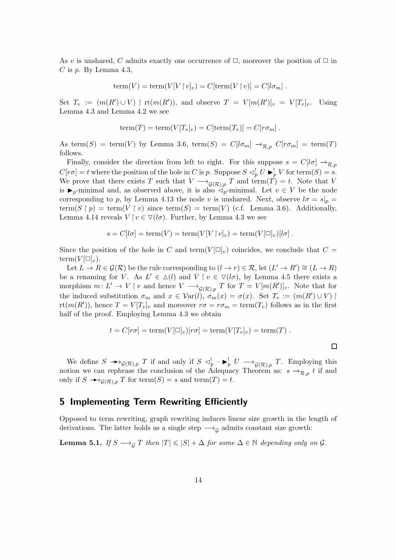
notion we can rephrase the conclusion of the Adequacy Theorem as: s −→R,p t if andonly if S ⊳−→G(R),p T for term(S) = s and term(T ) = t.

5 Implementing Term Rewriting Efficiently

Opposed to term rewriting, graph rewriting induces linear size growth in the length ofderivations. The latter holds as a single step −→G admits constant size growth:

Lemma 5.1. If S −→G T then |T | 6 |S|+∆ for some ∆ ∈ N depending only on G.

14

Proof. Set ∆ := max|R| | (L→ R) ∈ G and the lemma follows by definition.

It is easy to see that a graph rewrite step S −→G T can be performed in time poly-nomial in the size of the term graph S. By the above lemma we obtain that S can benormalised in time polynomial in |S| and the length of derivations. In the following,we prove a result similar to Lemma 5.1 for the relation ⊳−→G, where (restricted) foldingand unfolding is incorporated. The main obstacle is that due to unfolding, size growthof ⊳−→G is not bound by a constant in general. We now investigate into the relation ⊳p

and p.

Lemma 5.2. Let S be a term graph and let p a position in S.

1) If S ⊳ℓp T then ℓ 6 |p| and |T | 6 |S|+ |p|.

2) If S ℓp T then ℓ 6 |S p| and |T | 6 |S|.

Proof. We consider the first assertion. For term graphs U , let PU = w | PosU (w) =q and q 6 p be the set of unshared nodes above p. Consider U ⊳p V . Observe thatPU ⊂ PV holds: By definition U ⊏u

v V where PosV (u) = q with q 6 p. Clearly,PU ⊆ PV , but moreover u ∈ PV whereas u 6∈ PU . Hence for (S ⊳ℓ

p T ) = S = S0 ⊳p

. . . ⊳p Sℓ = T , we observe PS = PS0 ⊂ . . . PSℓ= PT . Note that |PS | > 1 since

rt(S) ∈ Ps. Moreover, |PT | = |p|+ 1 since the node corresponding to p in T is unshared(c.f. Lemma 4.13). Thus from PSi

⊂ PSi+1 (0 6 i < ℓ) we conclude ℓ 6 |p|. Next, wesee |T | 6 |S|+ |p| as |T | = |S|+ ℓ by definition of ⊳p.

We now prove the second assertion. Consider term graphs U and V such that U p V .By definition U ⊐u

v V where nodes u and v are strictly below position p in U . HenceU >m V for the morphism m underlying ⊐u

v . As a simple consequence of Lemma 3.4,we obtain U p >m V p and thus |U p| > |V p|. From this we conclude the lemma asabove, where for |T | 6 |S| we employ that if U ⊐u

v V then |V p| = |U p| − 1.

By combining the above two lemmas we derive the following:

Lemma 5.3. If S ⊳−→G T then |T | 6 |S|+dp(S)+∆ and dp(T ) 6 dp(S)+∆ for some∆ ∈ N depending only on G.

Proof. Consider S ⊳−→G T , i.e., S ⊳!p U !

p V −→G T for some position p and termgraphs U and V . Lemma 5.2 reveals |U | 6 |S| + |p| and further |V | 6 |U | for ∆ :=max|R| | (L→ R) ∈ G. As |p| 6 dp(S) we see |V | 6 |S| + dp(S). Since V −→G Timplies |T | 6 |V | + ∆ (c.f. Lemma 5.1) we establish |T | 6 |S| + dp(S) + ∆. Finally,dp(T ) 6 dp(S) + ∆ follows from the easy observation that both U ⊳p V and U p Vimply dp(U) = dp(V ), likewise V −→G T implies dp(T ) 6 V +∆.

Lemma 5.4. If S ⊳−→ℓG T then |T | 6 (ℓ+ 1)|S| + ℓ2∆ for ∆ ∈ N depending only on G.

Proof. We prove the lemma by induction on ℓ. The base case follows trivially, so supposethe lemma holds for ℓ, we establish the lemma for ℓ + 1. Consider a derivation S ⊳−→ℓ

G

15

T ⊳−→G U . By induction hypothesis, |T | 6 (ℓ + 1)|S| + ℓ2∆. Iterative application ofLemma 5.3 reveals dp(T ) 6 dp(S) + ℓ∆. Thus

|U | 6 |T |+ dp(T ) + ∆

6(

(ℓ+ 1)|S|+ ℓ2∆)

+(

dp(S) + ℓ∆)

+∆

6 (ℓ+ 2)|S| + ℓ2∆+ ℓ∆+∆

6 (ℓ+ 2)|S| + (ℓ+ 1)2∆ .

In the sequel, we prove that an arbitrary graph rewrite step S ⊳−→ T can be performedin time cubic in the size of S. Lemma 5.4 then allows us to lift the bound on steps to apolynomial bound on derivations in the size of S and the length of derivations. We closelyfollow the notions of [10]. As model of computation we use k-tape Turing Machines (TMfor short) with dedicated input- and output-tape. If not explicitly mentioned otherwise,we will use deterministic TMs. We say that a (possibly nondeterministic) TM computesa relation R ⊆ Σ∗ × Σ∗ if for all (x, y) ∈ R, on input x there exists an accepting runsuch that y is written on the output tape.

We fix a standard encoding for term graphs S. We assume that for each functionsymbol f ∈ F a corresponding tape-symbols is present. Nodes and variables are repre-sented by natural numbers, encoded in binary notation and possibly padded by zeros.We fix the invariant that natural numbers 1, . . . , |S| are used for nodes and variablesin the encoding of S. Thus variables (nodes) of S are representable in space O(log(|S|)).Finally, term graphs S are encoded as a ordered list of node specifications, i.e., triples ofthe form 〈v,L(v),Succ(v)〉 for all v ∈ S (compare [15, Section 13.3]). We call the entriesof a node specification node-field, label-field and successor-field respectively. We addi-tionally assume that each node specification has a status flag (constant in size) attached.For instance, we use this field below to mark subgraphs.

For a suitable encoding of tuples and lists, a term graph S is representable in sizeO(log(|S|) ∗ |S|). For this, observe that the length of Succ(v) is bound by the maximalarity of the fixed signature F . In this spirit, we define the representation size of a termgraph S as ‖S‖ := O(log(|S|) ∗ |S|).

Before we investigate into the computational complexity of ⊳−→, we prove some aux-iliary lemmas.

Lemma 5.5. The subgraph S u of S can be marked in quadratic time in ‖S‖.

Proof. We use a TM that operates as follows: First, the graph S is copied from the inputtape to a working tape. Then the node specifications of v ∈ S u are marked in a breath-first manner. Finally the resulting graph is written on the output tape. In order to marknodes two flags are employed, the permanent and the temporary flag. A node v is markedpermanent by marking its node specification permanent, and all node specifications ofSucc(v) temporary. Initially, u is marked. Afterward, the machine iteratively markstemporary marked node permanent, until all nodes are marked permanent.

16

Notice that a node v can be marked in time linear in ‖S‖. For that, the flag of thenode specification of v is set appropriately, and Succ(v) is copied on a second workingtape. Then S is traversed, and the node-field of each encountered node specification iscompared with the current node written on the second working. If the nodes coincide,then the flag of the node specification is adapted, the pointer on the second workingtape advances to the next node, and the process is repeated. Since the length of Succ(v)is bounded by a constant (as F is fixed), marking a node requires a constant numberof iterations. Since the machine marks at most |S| 6 ‖S‖ nodes we obtain an overallquadratic time bound in ‖S‖.

Lemma 5.6. Let S be a term graph and let p a position in S. A term graph T suchthat S ⊳!

p T is computable in time O(‖S‖2).

Proof. Given term graph S, we construct a TM that produces a term graph T suchthat S ⊳!

p T in time quadratic in ‖S‖. For that, the machine traverse S along thepath induced by p and introduces a fresh copy for each shared node encountered alongthat path. The machine has four working tapes at hand. On the first tape, the graphS is copied in such a way that nodes are padded sufficiently by leading zero’s so thatsuccessors can be replaced by fresh nodes u 6 2 ∗ |S| inplace. The graph represented onthe first tape is called the current graph, its size will be bound by O ‖S‖ at any time.On the second tape the position p, encoded as list of argument positions, is copied. Theargument position referred by the tape-pointer is called current argument position andinitially set to the first position. The third tape holds the current node, initially the rootrt(S) of S. Finally, the remaining tape holds the size of the current graph in binary, thecurrent size. One easily verifies that these preparatory steps can be done in time linearin S.

The TM now iterates the following procedure, until every argument position in pwas considered. Let v be the current node, let Si the current graph and let i be thecurrent argument position. We machine keeps the invariant that v is unshared in Si.

First, the node vi with vi vi in Si is determined in time linear in ‖S‖, the current

node is replaced by vi. Further, the pointer on the tape holding p is advanced to thenext argument position. Since v is unshared, vi is shared if and only if vi ∈ Succ(u)for u 6= v. The machine checks whether vi is shared in the current graph, by the aboveobservation in time linear in ‖S‖. If vi is unshared, the machine enters the next iteration.Otherwise, the node vi is cloned in the following sense. First, the the i-th successor viof v is replaced by a fresh node u. The fresh node is obtained by increasing the currentnode by one, this binary number is used as fresh node u. Further, the node specification〈u,L(vi),Succ(vi)〉 is appended to the current graph Si. Call the resulting graph Si+1.Then Si ⊏

uviSi+1 with PosSi+1(u) = q and q 6 p, i.e., Si ⊳p Si+1.

When the procedure stops, the machine has computed S = S0 ⊳p S1 ⊳p . . . ⊳p Sn =T . One easily verifies that Sn is ⊳p-minimal as every considered node along the path pis unshared. Each iteration takes time linear in ‖S‖. As as at most |p| 6 |S| iterationshave to be performed, we obtain the desired bound.

17

Lemma 5.7. Let S be a term graph and p a position in S. The term graph T such thatS !

p T is computable in time O(‖S‖2).

Proof. Define the height htU (u) of a node u in a term graph U inductively as usual:htU (u) := 0 if Succ(u) = [] and htU (v) := 1 + maxv∈Succ(u) htU (v) otherwise. We dropthe reference to the graph U when referring to the height of nodes in the analysis ofthe normalising sequence S !

p T below. This is justified as the height of nodes remainstable under ⊐-reductions.

Recall the definition of p: U p V if there exist nodes u, v strictly below p withU ⊐u

v V . Clearly, for u, v given, the graph V is constructable from U in time linear in|U |. However, finding arbitrary nodes u and v such that U ⊐u

v V takes time quadratic in|U | worst case. Since up to linear many ⊐-steps in |S| need to be performed, a straightforward implementation admits cubic runtime complexity. To achieve a quadratic boundin the size of the starting graph S, we construct a TM that implements a bottom upreduction-strategy. More precise, the machine implements the maximal sequence

S = S1 ⊐!u1

S2 ⊐!u2· · · ⊐!

uℓ−1Sℓ (a)

satisfying, for all 1 6 i < ℓ − 1, (i) either ht(ui) = ht(ui+1) and u ≺ v or ht(ui) <ht(ui+1), and (ii) for Si ⊐

vi,1ui . . . ⊐

vi,kui Si+1, ui and vi,j (1 6 j 6 k) are strictly below p.

By definition S ∗p Sℓ, it remains to show that the sequence (a) is normalising, i.e., Sℓ

is p-minimal. Set d := dp(S p) and define, for 0 6 h 6 d,

⊐(h) :=⋃

u,v∈Sp∧ht(v)=h

⊐uv .

Observe that each ⊐ui-step in the sequence (a) corresponds to a step ⊐(h) for some

0 6 h 6 d. Moreover, it is not difficult to see that

S = Si0 ⊐!(0) Si1 ⊐!

(1) · · · ⊐!(d) Sid+1

= Sℓ (b)

for Si0 , . . . , Sid+1 ⊆ S1, . . . , Sℓ−1.Next observe Si ⊐(h1)

Si+1 ⊐(h2)Si+2 and h1 > h2 implies Si ⊐(h2)

· ⊐(h1)Si+2:

suppose Si ⊐u′

u Si+1 ⊐v′

v Si+2 where ht(u) > ht(v) and u′, u, v, v′ ∈ S p, we showSi ⊐

v′

v · ⊐u′

u Si+2. Inspecting the proof of Lemma 4.10 we see ⊏u′

u · ⊐v′

v ⊆ ⊐v′

v · ⊏u′

u

for the particular case that u′, u, v and v′ pairwise distinct. The latter holds as ht(u′) =ht(u) 6= ht(v) = ht(v′). Hence it remains to show Si ⊐

v′

v S′i+1 for some term graph S′

i+1,or equivalently LSi

(v) = LSi(v′) and SuccSi

(v) = SuccSi(v′) by Lemma 4.9. The former

equality is trivial, for the latter observe ht(u′) = ht(u) > ht(v) = ht(v′) and thus neitheru′ 6∈ SuccSi

(v′) nor u′ 6∈ SuccSi(v). We see SuccSi

(v) = SuccSi+1(v) = SuccSi+1(v′) =

SuccSi(v′).

Now suppose that Sℓ is not p-minimal, i.e, Sℓ ⊐(h) U for some 0 6 h 6 d and termgraph U . But then we can permute steps in the reduction (b) such that Sih+1

⊐(h) V for

some term graph V . This contradicts ⊐!(h)-minimality of Sih+1

. We conclude that Sℓ isp-minimal. Thus sequence (a) is p-normalising.

18

We now construct a TM operating in time O(‖S‖2) that, on input S and p, computesthe sequence (a). We use a dedicated working tape to store the current graph Si. Initially,the term graph S is copied on this working tape. Further, the node w corresponding top in S is computed by recursion on p in time ‖S‖2. Afterward, the quadratic markingalgorithm of Lemma 5.5 is used to mark the subgraph S w in S.

The TM operates in stages, where in each stage the current graph Sih is replaced bySih+1

for Sih ⊐!(h) Sih+1

. Consider the subsequence

Sih = Sj1 ⊐!uj1· · · ⊐!

ujlSjl+1

= Sih+1(c)

of sequence (a) for j1 := ih and jl+1 := ih+1. Then h = ht(uj1) = · · · = ht(ujl). Callh the current height. To compute the above sequence efficiently, the TM uses the flagsdeleted, temporary and permanent besides the subterm marking. Let Sj (j1 6 j 6 jl+1)be the current graph. If a node u is marked deleted, it is treated as if u 6∈ Sj, thatis, when traversing Sj the corresponding node specification is ignored. Further, themachine keeps the invariant that when u ∈ Sj p then (the node specification of) uis marked permanent if and only if ht(u) < h. Thus deciding whether ht(u) = h forsome node u ∈ Si amounts to checking whether u is not marked permanent, but allsuccessors Succ(u) are marked permanent. To decide ht(u) = h solely based on thenode specification of u, the machine additionally record whether ui ∈ Succ(u) is markedpermanent in the node specification of u. Since the length of Succ(u) is bounded bya constant, this is can be done in constant space. At the beginning of each stage, themachine is in one of two states, say p and q (for current height h = 0, the initial stateis p).

- State p. In this state the machine is searching the next node uj to collapse. Itkeeps the invariant that previously considered nodes uji for j1 6 ji 6 i are markedtemporary. Reconsider the definition of the sequence (a). The node uj is the leastnode (with respect to > underlying ⊐) satisfying (i) uj is marked by the subtermmarking, and (ii) uj is not marked permanent but all nodes in Succ(uj) are markedpermanently, and (iii) uj is not marked temporary. Recall that node specificationsare ordered in increasing order. In order to find uj , the graph Sj is scanned fromtop to bottom, solely based on the node specification properties (i) — (iii) arechecked, and the first node satisfying (i) – (iii) is returned.

Suppose the node uj is found. The machine marks the node uj temporary andwrites uj, L(uj) and Succ(uj) on dedicated working tapes. Call uj the currentnode. The machine goes into state q as described below. On the other hand, it ujis not found, the stage is completed as all nodes of height h are temporary marked.The temporary marks, i.e., the marks of node uj1 , . . . , ujl are transformed intopermanent ones and the stage is completed. Notice that all nodes of height less orequal to h are marked permanent this way. The invariant on permanent marks isrecovered, the machine enters the next stage.

One verifies that one transition from state p requires at most linearly many stepsin ‖S‖.

19

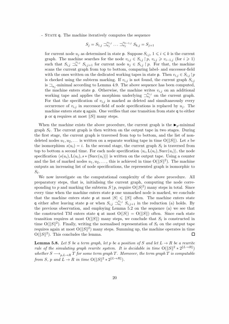
- State q. The machine iteratively computes the sequence

Sj = S1,j ⊐v1,juj . . . ⊐

vk−1,juj Sk,j = Sj+1

for current node uj as determined in state p. Suppose Si,j, 1 6 i 6 k is the currentgraph. The machine searches for the node vi,j ∈ Si,j p, vi,j > vi−1,j (for i > 1)such that Si,j ⊐

vi,ju Si,j+1 for current node uj ∈ Si,j p. For that, the machine

scans the current graph from top to bottom, comparing label- and successor-fieldwith the ones written on the dedicated working tapes in state p. Then vi,j ∈ Si,j pis checked using the subterm marking. If vi,j is not found, the current graph Si,j

is ⊐uj-minimal according to Lemma 4.9. The above sequence has been computed,

the machine enters state p. Otherwise, the machine writes vi,j on an additionalworking tape and applies the morphism underlying ⊐

vi,juj on the current graph.

For that the specification of vi,j is marked as deleted and simultaneously everyoccurrence of vi,j in successor-field of node specifications is replaced by uj . Themachine enters state q again. One verifies that one transition from state q to eitherp or q requires at most ‖S‖ many steps.

When the machine exists the above procedure, the current graph is the p-minimalgraph Sℓ. The current graph is then written on the output tape in two stages. Duringthe first stage, the current graph is traversed from top to bottom, and the list of non-deleted nodes u1, u2, . . . is written on a separate working tape in time O(‖S‖). Let s bethe isomorphism s(ui) = i. In the second stage, the current graph Sℓ is traversed fromtop to bottom a second time. For each node specification 〈ui,L(ui),Succ(ui)〉, the nodespecification 〈s(ui),L(ui), s ∗ (Succ(ui))〉 is written on the output tape. Using a counterand the list of marked nodes u1, u2, . . . , this is achieved in time O(‖S‖2). The machineoutputs an increasing list of node specifications, the represented graph is isomorphic toSℓ.

We now investigate on the computational complexity of the above procedure. Allpreparatory steps, that is, initialising the current graph, computing the node corre-sponding to p and marking the subterm S p, require O(|S|2) many steps in total. Sinceevery time when the machine enters state p one unmarked node is marked, we concludethat the machine enters state p at most |S| 6 ‖S‖ often. The machine enters stateq either after leaving state p or when Si,j ⊐

vi,jui Si,j+1 in the reduction (a) holds. By

the previous observation, and employing Lemma 5.2 on the sequence (a) we see thatthe constructed TM enters state q at most O(|S|) = O(‖S‖) often. Since each statetransition requires at most O(‖S‖) many steps, we conclude that Sℓ is constructed intime O(‖S‖2). Finally, writing the normalised representation of Sℓ on the output taperequires again at most O(‖S‖2) many steps. Summing up, the machine operates in timeO(‖S‖2). This concludes the lemma.

Lemma 5.8. Let S be a term graph, let p be a position of S and let L→ R be a rewriterule of the simulating graph rewrite system. It is decidable in time O(‖S‖2 ∗ 2‖L→R‖)whether S −→p,L→R T for some term graph T . Moreover, the term graph T is computable

from S, p and L→ R in time O(‖S‖2 ∗ 2‖L→R‖).

20

Proof. We construct a TM that on input S, p and L → R computes the reduct T forS −→p,L→R T . If the latter does not hold, the machine rejects. For this we suppose thatthe nodes of L → R are chosen in such a way that VL→R = 1, . . . , |L→ R| (we keepthis invariant when constructing the final algorithm). Let u be the node correspondingto p in S. In [3, Lemma 24] it is shown that there exists a TM operating in time2O(‖L‖) ∗O(‖S‖2) that, on input L, S and u, either writes on its output-tape the graphmorphism m such that m : L → S u if it exists, or fails. The morphism m is encodedas an associative list, more precisely, a list of pairs (u,m(u)) for u ∈ L. The size ofthis list is bound by O(|L| ∗ log(|L| + |S|)). First, this machine is used to computem : L → S u, the resulting morphism is stored on a working tape. For this, the nodeu is computed in time ‖S‖2 beforehand. If constructing the morphism fails, then ruleL→ R is not applicable at position p, i.e., u is not a redex in S with respect to L→ R.The constructed machine rejects. Otherwise, the reduct T is computed as follows.

Set L′ := r(L) and R′ := r(R) for the graph morphism r defined by r(v) := v + |S|.Then R′ ∩ S = ∅. We compute T = S[m′(R′)]u for m′ : L′ → S u using the morphismm : L → S u as computed above. Let f(v) = m(v) if LR(v) ∈ V and f(v) = v + |S|otherwise. Since VL ∩VR = VarR we see that T = S[f(R)]u.

Next, the machine constructs S∪f(R) on an additional working tape as follows. First,S is copied on this tape in time linear in ‖S‖. Simultaneously, |S| is computed on anadditional tape. Using the counter |S|, v+|S| is computable in time O(log(|R|)+log(|S|)),whereas m(v) for v ∈ L ∩ R = VarR is computable in time O(|L| ∗ log(|L| + |R|))(traversing the associative list representing m). We bind the complexity of f by O(‖L‖∗‖R‖∗‖S‖) independent on v. Finally, for each node-specification 〈v,L(v),Succ(v)〉 withL(v) ∈ F encountered in R, the machine appends 〈f(v),L(v), f∗(Succ(v))〉. EmployingL∩R = Var(R), one verifies that S ∪ f(R) is obtained this way. Overall, the runtime isO(‖L‖ ∗ ‖R‖2 ∗ ‖S‖).

Employing ‖f(R)‖ = O(|R| ∗ log(max(|R|, |S|))), we see that S ∪ f(R) can be boundin size by O(‖S‖ ∗ ‖R‖). To obtain T = (S ∪m(R′)) v = (S ∪ f(R)) v for v eitherrt(m(R′)) or rt(S), the quadratic marking algorithm of Lemma 5.5 is used. Finally, themarked subgraph obeying the standard encoding is written onto the output tape as inLemma 5.7.

We sum up: it takes at most 2O(‖L‖) ∗O(‖S‖2) many steps to compute the morphismm. The graph S∪m(R′) is obtained in time O(‖L‖∗‖R‖2∗‖S‖). Marking T in S∪m(R′)requires at most O(‖S ∪m(R′)‖2) = O(‖S‖2 ∗ ‖R‖2) many steps. Finally, the reduct Tis written in ‖S ∪ f(R)‖2 = O(‖S‖2 ∗ ‖R‖2) steps onto the output-tape. Overall, theruntime is bound by 2O(‖L‖) ∗O(‖S‖2 ∗ ‖R‖2) worst case.

Lemma 5.9. Let S be a term graph and let G(R) be the simulating graph rewrite systemof R. If S is not a normal-form of G(R) then there exists a position p and rule (L →R) ∈ G(R) such that a term graph T with S ⊳−→G(R),p,L→R T is computable in timeO(‖S‖3).

Proof. The TM searches for a rule (L→ R) ∈ G and position p such that S ⊳−→G(R),p,L→R

T for some term graph T . For this, it enumerates the rules (L→ R) ∈ G on a separate

21

working tape. For each rule L → R, each node u ∈ S and some p ∈ PosS it computesS1 such that S !

p S1 in time quadratic in ‖S‖2 (c.f. Lemma 5.7). Using the machine

of Lemma 5.8, it decides in time 2O(‖L‖) ∗ O(‖S1‖2) whether rule L → R applies to S1

at position p. Since R is fixed, 2O(‖L‖) is constant, thus the TM decides whether ruleL → R applies in time O(‖S1‖

2) = O(‖S‖2). Note that the choice of p ∈ PosS(u) isirrelevant, since S !

piS1 and S !

pjS2 for pi, pj ∈ PosS(u) implies S1

∼= S2. Hence thenode corresponding to pi in S1 is a redex with respect to L→ R if and only if the nodecorresponding to pj is. Suppose rule L→ R applies at S1 p. One verifies S1 p ∼= S2 pfor term graph S2 such that S ⊳!

p · !p S2. We conclude S ⊳−→G(R),p,L→R T for some

position p and rule (L→ R) ∈ G(R) if and only if the above procedure succeeds. Fromu one can extract some position p ∈ PosS(u) in time quadratic in ‖S‖. This can bedone for instance by implementing the function pos(u) = ε if u = rt(S) and pos(u) = pi

for some node v ∈ S with vi u and pos(v) = p. Overall, the position p ∈ PosS and

rule (L → R) ∈ G is found if and only if S ⊳−→p,L→R T for some term graph T . Since|S| 6 ‖S‖ nodes, and only a constant number of rules have to be checked, the overallruntime is O(‖S‖3).

To obtain T from S, p, and L → R, the machine now combines the machines fromLemma 5.6, Lemma 5.7 and Lemma 5.8. These steps can even be performed in timeO(‖S‖2), employing that the size of intermediate graphs is bound linear in the size of S(compare Lemma 5.2) and that sizes of (L→ R) ∈ G(R) are constant.

Lemma 5.10. Let S be a term graph and let ℓ := dl(S, ⊳−→G(R)). Suppose ℓ = Ω(|S|).

1) Some normal-form of S that is computable in deterministic time O(log(ℓ)3 ∗ ℓ7).

2) Any normal-form of S is computable in nondeterministic time O(log(ℓ)2 ∗ ℓ5).

Proof. We prove the first assertion. Consider the normalising derivation

S = T0 ⊳−→G(R) . . . ⊳−→G(R) Tl = T . (†)

where, for 0 6 i < l, Ti is obtained from Ti+1 as given by Lemma 5.9. By Lemma 5.4, wesee |Ti| 6 (ℓ + 1)|S| + ℓ2∆ = O(ℓ2). Here the latter equality follows by the assumptionℓ = Ω(|S|). Recall ‖Ti‖ = O(log(|Ti|)∗|Ti|) (0 6 i < l) and hence ‖Ti‖ = O(log(ℓ2)∗ℓ2) =O(log(ℓ) ∗ ℓ2). From this, and Lemma 5.9, we obtain that Ti+1 is computable from Ti

in time O(‖Ti‖3) = O(log(ℓ)3 ∗ ℓ6). Since l 6 dl(S, ⊳−→G(R)) = ℓ we conclude the first

assertion.We now consider the second assertion. Reconsider the proof Lemma 5.9. For a given

rewrite-position p, a step S ⊳−→G(R) T can be performed in time O(‖S‖). A nondeter-ministic TM can guess some position p, and verify whether the node corresponding to pis a redex in time O(‖S2‖). In total, the reduct T can be obtained in nondeterministictime O(‖S2‖). Hence, following the proof of the first assertion, one easily verifies thesecond assertion.

22

6 Discussion

We present an application of our result in the context of implicit computational com-plexity theory (see also [6, 5]).

Definition 6.1. Let N ⊆ Val be a finite set of non-accepting patterns. We call a termt accepting (with respect to N ) if there exists no p ∈ N such that pσ = t for somesubstitution σ. We say that R computes the relation R ⊆ Val×Val with respect to N ifthere exists f ∈ D such that for all s, t ∈ Val,

R(s, t) :⇐⇒ f(s) −→!R t and t is accepting .

On the other hand, we say that a relation R is computed by R if R is defined by theabove equations with respect to some set N of non-accepting patterns.

For the case that R is confluent we also say that R computes the (partial) functioninduced by the relation R.

The reader may wonder why we restrict to binary relations, but this is only a non-essential simplification that eases the presentation. The assertion that for normal-formst, t is accepting amounts to our notion of accepting run of a TRS R. This aims toeliminate by-products of the computation that should not be considered as part of therelation R. (A typical example would be the constant ⊥ if the TRS contains a rule ofthe form l →⊥ and ⊥ is interpreted as undefined.) The restriction that N is finite isessential for the simulation results below: If we implement the computation of R on aTM, then we also have to be able to effectively test whether t is accepting.

To compute a relation defined by R, we encode terms as graphs and perform graphrewriting using the simulating GRS G(R).

Theorem 6.2. Let R be a terminating TRS, moreover suppose rcR(n) = O(nk) forall n ∈ N and some k ∈ N, k > 1. The relations computed by R are computable innondeterministic time O(n5k+2). Further, if R is confluent then the functions computedby R are computable in deterministic time O(n7k+3). Here n refers to the size of theinput term.

Proof. We investigate into the complexity of a relation R computed by R. For that,single out the corresponding defined function symbol f and fix some argument s ∈ Val.Suppose the underlying set of non-accepting patterns is N . By definition, R(s, t) ifand only if f(s) −→!

R t and t ∈ Val is accepting with respect to N . Let S be a termgraph such that term(S) = f(s) and recall that |S| 6 |f(s)|. Set ℓ := dl(S, ⊳−→G(R)).

By the Adequacy Theorem 4.15, we conclude S ⊳−→!G(R) T where term(T ) = t, and

moreover, ℓ 6 rcR(|f(s)|) = O(nk). By Lemma 5.10 we see that T is computable from Sin nondeterministic time O(log(ℓ)2 ∗ℓ5) = O(log(nk)2 ∗n5k) = O(n5k+2). Clearly, we candecide in time linear in ‖T‖ = O(ℓ2) = O(n2k) (c.f. Lemma 5.4) whether term(T ) ∈ Val,further in time quadratic in ‖T‖ whether term(T ) is accepting. For the latter, weuse the matching algorithm of Lemma 5.8 on the fixed set of non-accepting patterns,where we employ pσ = term(T ) if and only if there exists a morphism m : P → T for

23

P ∈ (p) (c.f. Lemma 4.5 and Lemma 3.5). Hence overall, the accepting conditioncan be checked in (even deterministic) time O(n4k). If the accepting condition fails, theTM rejects, otherwise it accepts a term graph T representing t. The machine does soin nondeterministic time O(n5k+2) in total. As s was chosen arbitrary, we conclude thefirst half of the theorem.

Finally, the second half follows by identical reasoning, where we use the deterministicTM as given by 5.10 instead of the nondeterministic one.

Let R be a binary relation such that R(x, y) can be decided by some nondeterministicTM in time polynomial in the size of x. The function problems RF associated withR is: given x, find some y such that R(x, y) holds. The class FNP is the class of allfunctional problems defined in the above way, compare [13]. FP is the subclass resultingif we only consider function problems in FNP that can be solved in polynomial time bysome deterministic TM. As by-product of Theorem 6.2 we obtain:

Corollary 6.3. Let R be a terminating TRS with polynomially bounded runtime com-plexity. Suppose R computes the relation R. Then RF ∈ FNP for the function problemRF associated with R. Moreover, if R is confluent then RF ∈ FP.

Proof. The nondeterministic TM M as given by Theorem 6.2 (the deterministic TMM , respectively) can be used to decide membership (s, t) ∈ R. Observe that by theassumptions on R, the runtime of M is bounded polynomially in the size of s. Recallthat s is represented as some term graph S with term(S) = s, in particular s is encodedover the alphabet of M in size ‖S‖ = O(log(|S|) ∗ |S|) for |S| 6 |s|. Thus trivially Moperates in time polynomially in the size of S.

References

[1] M. Avanzini and G. Moser. Complexity Analysis by Rewriting. In Proc. of 9thFLOPS, volume 4989 of LNCS, pages 130–146. Springer Verlag, 2008.

[2] M. Avanzini and G. Moser. Dependency Pairs and Polynomial Path Orders. InProc. of 20th RTA, volume 5595 of LNCS, pages 48–62. Springer Verlag, 2009.

[3] M. Avanzini and G. Moser. Complexity Analysis by Graph Rewriting. In Proc. of11th FLOPS, LNCS. Springer Verlag, 2010. To appear.

[4] F. Baader and T. Nipkow. Term Rewriting and All That. Cambridge UniversityPress, 1998.

[5] U. Dal Lago and S. Martini. Derivational Complexity is an Invariant Cost Model.In Proc. of 1st FOPARA, 2009.

[6] U. Dal Lago and S. Martini. On Constructor Rewrite Systems and the Lambda-Calculus. In Proc. of 36th ICALP, volume 5556 of LNCS, pages 163–174. SpringerVerlag, 2009.

24

[7] J. Endrullis, J. Waldmann, and H. Zantema. Matrix Interpretations for ProvingTermination of Term Rewriting. JAR, 40(3):195–220, 2008.

[8] A. Koprowski and J. Waldmann. Arctic Termination . . . Below Zero. In Proc. of19th RTA, volume 5117 of LNCS, pages 202–216. Springer Verlag, 2008.

[9] M. Korp and A. Middeldorp. Match-bounds revisited. IC, 207(11):1259–1283, 2009.

[10] Dexter C. Kozen. Theory of Computation. Springer Verlag, first edition, 2006.

[11] G. Moser and A. Schnabl. The Derivational Complexity Induced by the DependencyPair Method. In Proc. of 20th RTA, volume 5595 of LNCS, pages 255–260. SpringerVerlag, 2009.

[12] G. Moser, A. Schnabl, and J. Waldmann. Complexity Analysis of Term RewritingBased on Matrix and Context Dependent Interpretations. In Proc. of 28th FST-TICS, pages 304–315. Schloss Dagstuhl - Leibniz-Zentrum fuer Informatik, Ger-many, 2008.

[13] Christos H. Papadimitriou. Computational Complexity. Addison Wesley Longman,second edition, 1995.

[14] D. Plump. Essentials of Term Graph Rewriting. ENTCS, 51:277–289, 2001.

[15] TeReSe. Term Rewriting Systems, volume 55 of Cambridge Tracks in TheoreticalComputer Science. Cambridge University Press, 2003.

25