Technical Report Documentation Page 1. Report No. 2 ... traffic control is a common intersection...

i

Technical Report Documentation Page 1. Report No.

SWUTC/15/600451-00113-1

2. Government Accession No.

3. Recipient's Catalog No.

4. Title and Subtitle

MANUAL TRAFFIC CONTROL FOR PLANNED SPECIAL

EVENTS AND EMERGENCIES

5. Report Date

November 2015 6. Performing Organization Code

7. Author(s)

Scott Parr and Brian Wolshon

8. Performing Organization Report No.

Report 600451-00113-1 9. Performing Organization Name and Address Gulf Coast Center for Evacuation and Transportation Resiliency

Department of Civil and Environmental Engineering

Louisiana State University

Baton Rouge, LA 70803

10. Work Unit No. (TRAIS)

11. Contract or Grant No.

DTRT12-G-UTC06

12. Sponsoring Agency Name and Address

Southwest Region University Transportation Center

Texas A&M Transportation Institute

Texas A&M University System

College Station, Texas 77843-3135

13. Type of Report and Period Covered

14. Sponsoring Agency Code

15. Supplementary Notes

Supported by a grant from the U.S. Department of Transportation, University Transportation Centers

Program.

16. Abstract

Manual traffic control is a common intersection control strategy in which trained personnel,

typically police law enforcement officers, allocate intersection right-of-way to approaching vehicles.

Manual intersection control is a key part of managing traffic during emergencies and planned special

events. Despite the long history of manual traffic control throughout the world and its assumed

effectiveness, there have been no quantitative, systematic studies of when, where, and how it should be

used or compared to traditional traffic control devices.

The goal of this research was to quantify the effect of manual traffic control on intersection

operations and to develop a quantitative model to describe the decision-making of police officers directing

traffic for special events and emergencies. This was accomplished by collecting video data of police

officers directing traffic at several special events in Baton Rouge, LA and Miami Gardens, FL. These data

were used to develop a discrete choice model (logit model) capable of estimating police officer’s choice

probabilities on a second-by-second basis. This model was able to be programmed into a microscopic

traffic simulation software system to serve as the signal controller for the study intersections, effectively

simulating the primary control decision activities of the police officer directing traffic. The research

findings suggested police officers irrespective of their location, tended to direct traffic in a similar fashion;

extending green time for high demand directions while avoiding gaps in the traffic stream.

17. Key Words

Manual Traffic Control, Emergency Evacuation,

Microsimulation, Logit Model

18. Distribution Statement

No restrictions. This document is available to the

public through NTIS:

National Technical Information Service

5285 Port Royal Road

Springfield, Virginia 22161 19. Security Classif.(of this report)

Unclassified

20. Security Classif.(of this page)

Unclassified

21. No. of Pages

120

22. Price

Form DOT F 1700.7 (8-72) Reproduction of completed page authorized

ii

iii

MANUAL TRAFFIC CONTROL FOR PLANNED SPECIAL EVENTS AND

EMERGENCIES

by

Scott Parr, Ph.D., E.I.T. Associate Director of Research

Gulf Coast Center for Evacuation and Transportation Resiliency



3502B Patrick F. Taylor Hall


Phone: (225) 578-9165

Email: [email protected]

Brian Wolshon, Ph.D., P.E., PTOE

Director and Professor

Gulf Coast Center for Evacuation and Transportation Resiliency



3502A Patrick F. Taylor Hall


Phone: (225) 578-5247

Email: [email protected]

SWUTC Project No. 600451-000113

conducted for

Southwest Region University Transportation Center

November 2015

mailto:[email protected]

mailto:[email protected]

iv

v

DISCLAIMER

The contents of this report reflect the views of the authors, who are responsible for the facts

and the accuracy of the information presented herein. This document is disseminated under the

sponsorship of the U.S. Department of Transportation’s University Transportation Centers Program,

in the interest of information exchange. The U.S. Government assumes no liability for the contents or

use thereof.

vi

ACKNOWLEDGEMENTS

The authors gratefully acknowledges the financial support of the Gulf Coast Center for

Evacuation and Transportation Resiliency; a United States Department of Transportation

sponsored University Transportation Center and part of the Southwest University Transportation

Center (SWUTC).

vii

EXECUTIVE SUMMARY

Manual traffic control is a common intersection control strategy in which trained

personnel, typically police law enforcement officers, allocate intersection right-of-way to

approaching vehicles. Manual intersection control is a key part of managing traffic during

emergencies and planned special events. It is widely assumed that the flow of traffic through

intersections can be greatly improved by the direction given from police officers who can

observe and respond to change conditions by allocating green time to the approaches that require

it the most. Despite the long history of manual traffic control throughout the world and its

assumed effectiveness, there have been no quantitative, systematic studies of when, where, and

how it should be used or compared to more traditional traffic control devices.

The goal of this research was to quantify the effect of manual traffic control on

intersection operations and to develop a quantitative model to describe the decision-making of

police officers directing traffic for special events and emergencies. This was accomplished by

collecting video data of police officers directing traffic at several special events in Baton Rouge,

LA and Miami Gardens, FL. These data were used to develop a discrete choice model (logit

model) capable of estimating police officer’s choice probabilities on a second-by-second basis.

This model was able to be programmed into a microscopic traffic simulation software system to

serve as the signal controller for the study intersections, effectively simulating the primary

control decision activities of the police officer directing traffic. The research findings suggested

police officers irrespective of their location, tended to direct traffic in a similar fashion;

extending green time for high demand directions while attempting to avoid long gaps or waste in

the traffic stream. This indicates that when officers are placed in similar situation they are likely

to make the same primary control decisions.

viii

TABLE OF CONTENTS

LIST OF TABLES .......................................................................................................................... x

LIST OF FIGURES ...................................................................................................................... xii

CHAPTER 1. INTRODUCTION ................................................................................................... 1

1.1 Problem Statement ................................................................................................................ 2

1.1.1 Police Implementation ................................................................................................... 2

1.2 Research Need ...................................................................................................................... 3

1.3 Research Goals and Objectives ............................................................................................. 4

CHAPTER 2. BACKGROUND ..................................................................................................... 6

2.1 History of Traffic Control ..................................................................................................... 7

2.2 Manual of Uniform Traffic Control Devices (MUTCD) .................................................... 19

2.3 Police Training For Traffic Control .................................................................................... 21

2.3.1 Northwestern University Traffic Institute .................................................................... 21

2.3.2 Modern Police Training for Traffic Control ................................................................ 23

2.4 Technical Manuals, Handbooks and Published Guidelines ................................................ 25

2.5 Special Event and Emergency Planning ............................................................................. 26

2.5.1 Special Event Planning ................................................................................................ 26

2.5.2 Emergency Planning .................................................................................................... 27

2.6 Manual Traffic Control and Empirical Studies ................................................................... 28

2.7 Summary of Literature Review Findings ............................................................................ 32

CHAPTER 3. METHODOLOGY ................................................................................................ 35

3.1 Data Collection and Reduction ........................................................................................... 35

3.1.1 Data Collection Device ................................................................................................ 40

3.1.2 Data Reduction............................................................................................................. 45

3.1.3 General Observations ................................................................................................... 47

3.2 Discrete Choice Modeling .................................................................................................. 48

3.2.1 Discrete Choice ............................................................................................................ 49

3.2.2 Discrete Choice Model Selection ................................................................................. 51

3.2.3 Utility Function ............................................................................................................ 52

3.2.4 Model Goodness-of-Fit ................................................................................................ 54

3.3 Simulation Modeling .......................................................................................................... 56

3.3.1 Simulation Model Building.......................................................................................... 56

CHAPTER 4.0 LOGIT MODEL ANALYSIS ............................................................................. 60

4.1 Variable Selection ............................................................................................................... 61

ix

4.2 Logit Model Estimation ..................................................................................................... 64

4.2.1 The Constant Variable ................................................................................................. 65

4.2.2 Primary ......................................................................................................................... 66

4.2.3 Secondary ..................................................................................................................... 68

4.2.4 Tertiary ......................................................................................................................... 69

4.2.5 Quaternary.................................................................................................................... 70

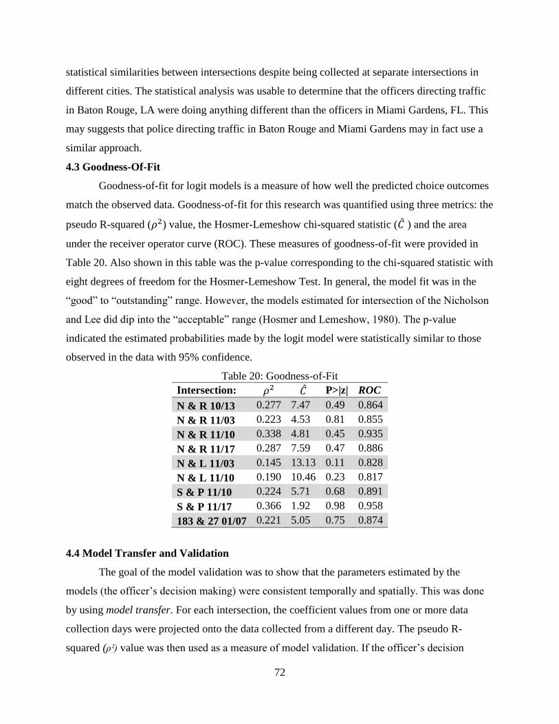
4.3 Goodness-Of-Fit ................................................................................................................. 72

4.4 Model Transfer and Validation ........................................................................................... 72

4.4.1 Validation Results ........................................................................................................ 74

4.5 Summary of Logit Model Findings..................................................................................... 75

CHAPTER 5. SIMULATION MODEL ANALYSIS .................................................................. 77

5.1 Simulation Model Calibration............................................................................................. 77

5.1.1 Vehicle Demand Calibration ........................................................................................ 78

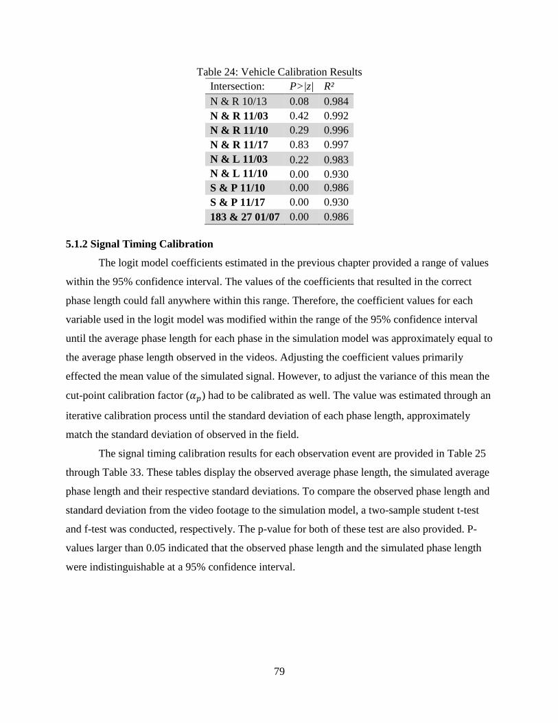
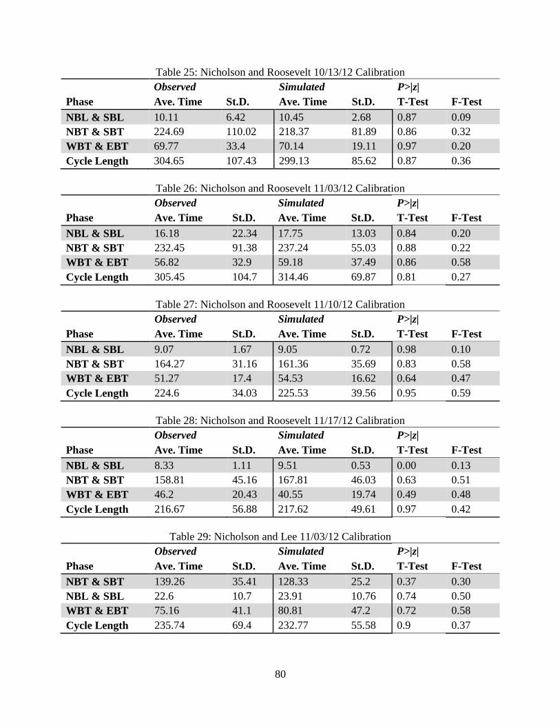
5.1.2 Signal Timing Calibration............................................................................................ 79

5.2 Validation ............................................................................................................................ 82

5.3 Comparative analysis .......................................................................................................... 84

5.3.1 Total Throughput ......................................................................................................... 84

5.3.2 Signal Timing............................................................................................................... 85

5.4 Summary of Simulation Model Findings ............................................................................ 92

CHAPTER 6. CONCLUSION...................................................................................................... 93

6.1 Future Work ........................................................................................................................ 95

6.1.1 Technology Development ............................................................................................ 95

6.1.2 Traffic Simulation Tools .............................................................................................. 96

REFERENCES ............................................................................................................................. 97

APPENDIX A. INTERSECTION GEOMETRIC DESIGN ...................................................... 105

x

LIST OF TABLES

Table 1: Research Objectives and Performance Metric .................................................................. 5

Table 2: Advantages and Disadvantages for Manual Traffic Control (Marsh, 1927) .................. 16

Table 3: Advantages and Disadvantages for Automated Signal Control (Marsh, 1927).............. 17

Table 4: Data Collection ............................................................................................................... 40

Table 5: Data Collection Equipment Cost (US Dollars) ............................................................... 41

Table 6: Sample Intersection Event Time-Line ............................................................................ 46

Table 7: Data Partition .................................................................................................................. 47

Table 8: Variable Description ....................................................................................................... 63

Table 9: Data Coding Example ..................................................................................................... 64

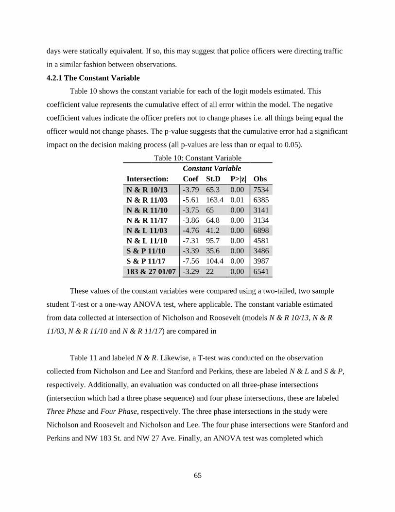
Table 10: Constant Variable ......................................................................................................... 65

Table 11: Statistical Testing for the Constant Variable ................................................................ 66

Table 12: Primary Direction ......................................................................................................... 67

Table 13: Statistical Testing for the Primary Direction ................................................................ 68

Table 14: Secondary Direction ..................................................................................................... 68

Table 15: Statistical Testing for Secondary Direction .................................................................. 69

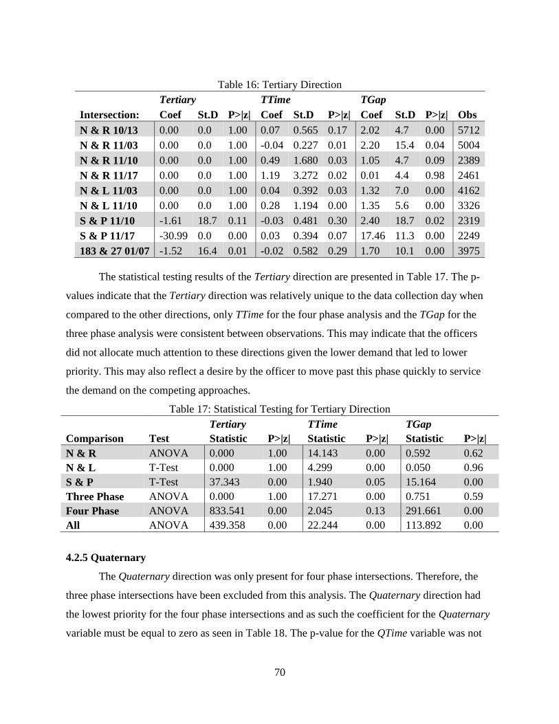
Table 16: Tertiary Direction ......................................................................................................... 70

Table 17: Statistical Testing for Tertiary Direction ...................................................................... 70

Table 18: Quaternary Direction .................................................................................................... 71

Table 19: Statistical Testing for the Quaternary Direction ........................................................... 71

Table 20: Goodness-of-Fit ............................................................................................................ 72

Table 21: Validation Partition ....................................................................................................... 73

Table 22: Nicholson and Roosevelt Combined Logit Model ....................................................... 74

Table 23: Logit Model Validation Results .................................................................................... 75

Table 24: Vehicle Calibration Results .......................................................................................... 78

Table 25: Nicholson and Roosevelt 10/13/12 Calibration ............................................................ 80




Table 29: Nicholson and Lee 11/03/12 Calibration ...................................................................... 80

Table 30: Nicholson and Lee 11/10/12 Calibration ...................................................................... 81

xi

Table 31: Stanford and Perkins 11/10/12 Calibration................................................................... 81

Table 32: Stanford and Perkins 11/17/12 Calibration................................................................... 81

Table 33: NW 183 St. and NW 27 Ave. 01/07/13 Calibration ..................................................... 81

Table 34: Vehicle Validation ........................................................................................................ 83

Table 35: Nicholson and Roosevelt Signal Validation ................................................................. 83

Table 36: Nicholson and Lee Signal Validation ........................................................................... 83

Table 37: Stanford and Perkins Signal Validation ........................................................................ 83

Table 38: NW 183 St. and NW 27 Ave. Signal Validation .......................................................... 84

Table 39: Intersection Throughput Volumes ................................................................................ 85

Table 40: Nicholson and Roosevelt 10/13/12 Actuated Signal Timing ....................................... 85




Table 44: Nicholson and Lee 11/03/12 Actuated Signal Timing ................................................. 86

Table 45: Nicholson and Lee 11/10/12 Actuated Signal Timing ................................................. 86

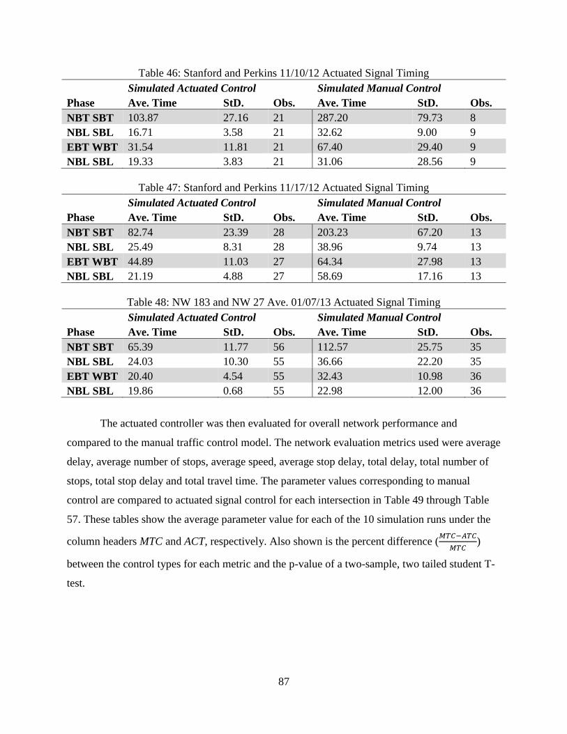
Table 46: Stanford and Perkins 11/10/12 Actuated Signal Timing .............................................. 87

Table 47: Stanford and Perkins 11/17/12 Actuated Signal Timing .............................................. 87

Table 48: NW 183 and NW 27 Ave. 01/07/13 Actuated Signal Timing ...................................... 87

Table 49: Nicholson and Roosevelt 10/13/12 Network Performance .......................................... 88




Table 53: Nicholson and Lee 11/03/12 Network Performance .................................................... 89

Table 54: Nicholson and Lee 11/10/12 Network Performance .................................................... 89

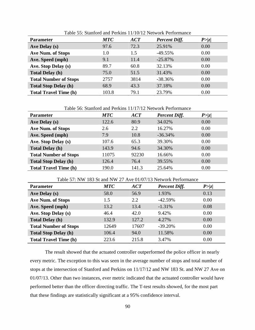
Table 55: Stanford and Perkins 11/10/12 Network Performance ................................................. 90

Table 56: Stanford and Perkins 11/17/12 Network Performance ................................................. 90

Table 57: NW 183 St and NW 27 Ave 01/07/13 Network Performance...................................... 90

xii

LIST OF FIGURES

Figure 1: Semaphore Police Notice (Copyright University of London) ......................................... 9

Figure 2: Police Signal Coordination Cartoon (Marsh, 1927) ...................................................... 10

Figure 3: Traffic Crowsnest Schematic (Eno, 1920) .................................................................... 11

Figure 4: Detroit Traffic Crowsnest (Eno, 1920).......................................................................... 12

Figure 5: Four Direction Three Bulb Traffic Light (Henry Ford Museum) ................................. 13

Figure 6: Estimate of Automated Traffic Signal Controllers in the U.S. (Marsh, 1927) .............. 15

Figure 7: Methodology Flow Chart .............................................................................................. 36

Figure 8: Baton Rouge, LA Study Area........................................................................................ 38

Figure 9: Miami Gardens, FL Study Area .................................................................................... 39

Figure 10: Data Collection Camera .............................................................................................. 42

Figure 11: Relative Camera Locations and Coverage Areas ........................................................ 43

Figure 12: Camera Platform Mounting ......................................................................................... 44

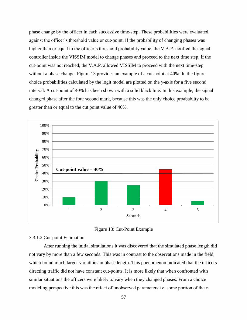
Figure 13: Cut-Point Example ...................................................................................................... 57

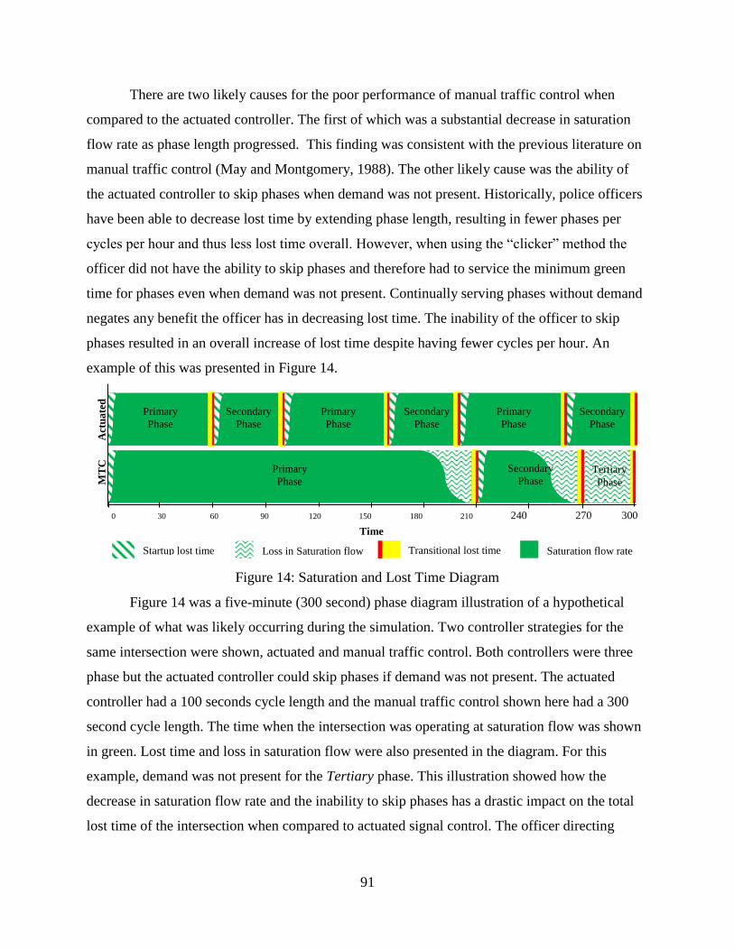
Figure 14: Saturation and Lost Time Diagram ............................................................................. 91

Figure 15: Geomtric Design of Stanford and Perkins ................................................................. 105

Figure 16: Geometric Design of Nicholson and Lee .................................................................. 106

Figure 17: Geometric Design of Nicholson and Roosevelt ........................................................ 107

Figure 18: Geometric Design of NW 183 St and NW 27 Ave ................................................... 108

1

CHAPTER 1. INTRODUCTION

Manual traffic control is a common intersection control strategy in which trained

personnel, typically police law enforcement officers, allocate intersection right-of-way to

approaching vehicles. The need for manual control is often associated with abnormally high,

unbalanced, or widely varying directional and intersecting traffic demand. Although such

conditions can occur at any time, they are particularly common before and after special events

and also associated with emergencies such as power outages and evacuations. Manual traffic

control has been effective under these conditions because police can directly observe and adapt

to the changing patterns of demand (Weston, 1996). In addition to being able to directly allocate

right-of-way at intersections in response to changing demand, police-conducted manual control

can also put “boots-on-the-ground” to observe conditions, respond to problems, and project the

presence of authority during times of crisis (Carson and Bylsma, 2003).

Manual traffic control has most often been used at high volume intersections and for

planned special events and emergencies at locations where traffic from one or more exit routes

merges or conflicts with traffic with another (Weston, 1996). It has generally been used to

minimize congestion, expedite emergency traffic, exclude unauthorized vehicle entries, and

protect the public (MUTCD, 2009). Depending on the amount of traffic, number of lanes

involved, and complexity of the location, as few as one and as many as several officers may be

required at a single intersection.

Manual traffic control has typically been conducted using one of two methods; the

traditional “officer in the intersection” approach and the more modern “clicker” method. The

“officer in the intersection” positions uniformed personnel near the center of the intersection,

directing vehicles and pedestrians using hand gestures. The advantages of this method are that it

is easy to deploy and can be used at any intersection with little to no preparation. The major

disadvantage is that it can be unsafe for the officer and is prone to inefficiencies in which

vehicles inevitably slow down and oftentimes completely stop to ask the operator questions on a

variety of subjects (Marsh, 1927; Weston, 1996). The “clicker” method enables a police officer

to allocate right-of-way by changing the phase length from the traffic signal controller. Operators

are able to change which approach directions will receive a green indication from the controller

with the “click” of a button. The advantages of this method are improved safety for the officer

and the elimination of the inefficiencies in flow caused by drivers slowing down to avoid the

2

officer standing in the intersection. However, this method can only be used at intersections with

properly equipped controller hardware and the operator must have a key to access the locked

control panel.

1.1 Problem Statement

In addition to their enforcement responsibilities, police personnel play many important roles

before, during, and after emergencies. These range from maintaining law and order; providing

security in impacted areas; serving as first responders for health and safety emergencies; and

conducting rescue operations (ESF#13, 2009). Despite its advantages during emergencies

manual traffic control exposes officers to unacceptable safety risks, requires significant

manpower, and may be a poor utilization of limited police resources during emergencies (Parr

and Kasiar, 2011). It is further suggested that conventional signal control can provide a safer,

more efficient, and more effective option for moving traffic. Based on these two conflicting

views, a disagreement exists among those who believe manual traffic control is an essential

element of special event and emergency traffic management and those who believe traffic would

flow more efficiently using conventional signal control. The discussion of whether manual

control is effective and when, where, and how it should be used, has not been systematically

quantified or scientifically studied. A review of the current state-of-practice has shown that the

administration, implementation and execution of manual traffic control have historically been

based on expert judgment, local knowledge, past experience, and, in some cases, public

perception. Furthermore, it is unknown whether manual traffic control is conducted in a uniform

manner across the country or even within the same state, county or locale.

1.1.1 Police Implementation

There are four basic levels of police jurisdiction, including Federal, State, County, and

City. It has been estimated that there are approximately 20,000 police agencies within the United

States, each of which conduct manual traffic control for highways on a regular basis using their

own set of policies and practices (USDOJ, 2008). It is particularly notable that none of these

20,000 police agencies have developed comprehensive guidelines or collected any best-practices

on the administration of manual traffic control. This is in contrast to the transportation

profession, where practices are more formalized and regulated through the publication of

guidelines, manuals, and procedures for practice. The terminology between police and

transportation officials also differs. Transportation professionals use the term “manual control”

3

or “manual traffic controls”, as defined in the Manual on Uniform Traffic Control Devices

(MUTCD, 2009). On the other hand, police literature typically uses “directing traffic” or “traffic

direction” to describe manual signal control (Weston, 1996).

As a result, no single universally recognized authoritative source or sets of guidelines that

govern manual traffic control currently exist. The manner in which an officer directs traffic and

allocates right-of-way has been virtually unstudied within the transportation community. For

example, no research has been conducted to date on the stimulus-response relationship between

operational traffic stream characteristics and officer decision-making while directing traffic.

Without an understanding of how and why police allocate green time, it is not possible to assess

the performance of manual traffic control from a systematic engineering point-of-view.

The current state-of-the-practice in evaluating traffic operations and control employs

traffic simulation modeling to assess conditions. However, due to the un-quantified nature of

manual traffic control, it has not been possible to accurately represent or calibrate simulation

models to fit empirical observations. As a result, current special event and emergency

evacuation simulations have been unable to realistically model the essence of neither manual

traffic control nor the results that are produced by it. Without this ability, the traffic management

plans developed for these situations cannot be tested in advance via traffic simulation.

1.2 Research Need

Many event traffic management plans and emergency traffic management plans call for

the use of manual traffic control in response to oversaturated traffic conditions. Expediting traffic

flow is a particularly high priority during emergencies when the effective movement of traffic

may be a matter of life and death. For example, the Nuclear Regulatory Commission (NRC)

suggests the use of manual traffic control to facilitate the evacuation of areas surrounding nuclear

power plants in the event of a disaster (NRC, 2011). However, during emergencies, police

personnel are also in great demand for other non-traffic related duties. During non-emergency

events, police presence can have a high economic cost because it often requires overtime or extra

duty pay. It is therefore essential to identify the benefits and costs, as well as the trade-offs,

advantages, and disadvantages associated with manual intersection traffic control.

There is also a need to quantify the operational effects of manual traffic control on

intersection performance. Allowing the performance of manual traffic control to be compared to

an actuated controller. This will enable the travel-time savings, if any from manual control to be

4

weighed against the cost of deploying the police officer at the intersection. Without such

comparisons, there can be no quantitative metric to evaluate manual control.

Under manual traffic control, police officers must make decisions of phase length and

phase sequence while directing traffic. By definition, these decisions have an impact on traffic

operations of the intersection. Thus, the actions taken by the officer have significant

consequences (both positive and negative) for potentially hundreds of people approaching the

intersection. It has been observed that the likelihood of inadequate green time allocation is

greater if the officer is inexperienced or has not been properly trained (Marsh, 1927). If an

officer provides inadequate green time to one phase of an intersection, the resulting queue can

propagate upstream interfering with the operations of adjoining intersections. Traffic simulation

is a relatively inexpensive tool used to evaluate proposed traffic management strategies for

effectiveness and efficiency. However, no simulation software has the ability to simulate the

effect that a police officer directing traffic has on roadway operations. It would be useful to

develop a simulation tool capable of effectively representing manual traffic control for the

purpose of evaluating traffic flow. Such a tool will help identify where, how and when manual

traffic control should be implemented to better utilize officer resources and intersection right-of-

way. With this tool, event planners would also be able to evaluate “what if” scenarios with

quantifiable results to aid in their decision-making. Furthermore, emergency managers will have

a better understanding of where to place police resources in the event of a catastrophe.

1.3 Research Goals and Objectives

The goal of this research was to quantify the effect of manual traffic control on

intersection operations and to develop a quantitative model to describe the decision-making of

police officers directing traffic for special events and emergencies. This was achieved by

collecting video data of police officers directing traffic at several special events in Baton Rouge,

LA and Miami Gardens, FL. The data was used to develop a discrete choice model (logit model)

to quantify the independent variables likely to effect an officer’s right-of-way allocation while

directing traffic. This model was programmed into a microscopic traffic simulation program,

VISSIM 5.3 to replace the signal controller logic for the study intersections. This had the effect

of simulating manual traffic control, which was then compared to the video footage collected in

the field for validation purposes. This model was used to compare the performance of the police

5

officer to a fully actuated traffic controller. The research objectives were summarized in Table 1.

A performance metric using proven quantifiable measures was created (when applicable).

Table 1: Research Objectives and Performance Metric

Order Objectives Performance Metric

1

Conduct a review of the existing body of

literature on manual traffic control from

both transportation and police research

perspectives

A literature review encompassing the

breadth and depth of knowledge in the field,

both state-of-the-art and state-of-the-

practice

2

Conduct a quantitative analysis of the

stimulus-response relationship between

the traffic stream and officers’ right-of-

way decisions while directing traffic

Traffic stream variables with strong and

weak correlation to observed officer actions

were measured using a p-value of 0.05 and

0.1, respectively

3 Simulate manual traffic control for the

intersections in the study

The performance of the simulation model

was compared to recorded videos using

regression analysis with R²-values no less

than 0.80 and comparison T-test/ANOVA

4

Evaluate the cost-benefit relationship

between manual traffic control and

automated traffic control

The traffic control measures are compared

using a two sample T-test analysis at ±5% at

95% confidence

The next chapter starts by reviewing and synthesizing relevant research, facts, and

opinions from the perspective of the police and transportation professions. The following chapter

describes the research methodology developed to address the problem statement and the existing

gaps in the literature. Chapter 4 and Chapter 5, discuss the discrete choice model results and the

application of the discrete choice model as a means of simulating manual traffic control,

respectively. The final chapter summarizes and concludes the research effort as well as providing

opportunities for future work.

6

7

CHAPTER 2. BACKGROUND

The design, implementation, and maintenance of traffic control devices in the United

States has been an evolutionary process. Police officers were the first true traffic control devices.

Over time, however, police officers were replaced by simple traffic signals which were

improved, later by the introducing advanced traffic control systems. For the development of this

research, several areas of literature were reviewed including the history of traffic control, police

traffic control training, manuals and handbooks, manual of uniform traffic control devices

(MUTCD), special event and emergency planning, and empirical studies on manual traffic

control.

2.1 History of Traffic Control

Traffic control began to emerge in London, England in the early 18th

century. As early as

1722, traffic control measures were taken to ensure swift movement of horse drawn carriages,

buggies, carts, and pedestrians across the London Bridge. At the time, crossing the bridge was

seen as an inconvenience due to the disorderly nature of the traffic movements. The Lord Mayor

organized a coalition of three men and appointed them as public servants to monitor and regulate

individuals crossing on the bridge. Their job was to keep traffic on the left side of the road and to

keep the traffic moving at all times (Paxton, 1969).

Traffic control in the United States dates back to the 1860’s when New York City’s

Police Department was assigned to manage the reckless driving of horse-drawn buses within the

city. This was in response to public outcry over the deaths of several pedestrians trampled by the

horse-drawn buses. The New York City Police Department assigned the tallest officers on the

force to the new squad to ensure that the officers could see over carriages and pedestrians. The

officers were known to point, wave, and shout to move traffic on the busy streets (Paxton, 1969).

The first traffic control device was introduced in London, England in 1868 at the

intersection opposite Palace Yard, near the House of Parliament. The device was a composite

semaphore signal with color coded gas lanterns for lights (green for go and red for stop). It was

built by railway signal engineers Saxby and Farmer of the London Brighton and South Coast

railway company. The semaphore consisted of three arm leavers, each facing one of the three

intersecting streets: Bridge Street, Great George Street, and Parliament Street.

To alert the traveling public of the new traffic control measure, the Metropolitan Police

printed 10,000 copies of a police notice seen in Figure 1. The police notice informed travelers

8

when the semaphore arms were lowered so by night, when the lantern was green, they could

proceed into the intersection with caution; meanwhile when the arms were raised or the lantern

burned red to stop.

By the Signal “CAUTION,” all persons in charge of Vehicles and Horses are warned to

pass over the Crossing with Care, and due regard to the safety of Foot Passengers. The

Signal “STOP,” will only be displayed when it is necessary that Vehicles and Horses

shall be actually stopped on each side of the Crossing to allow the passage of Persons on

Foot; notice being thus given to all persons in charge of Vehicles and Horses to stop clear

of the Crossing (University of London, 2013).

The semaphore was operated by a police constable and was considered a success. However, the

semaphore was soon removed due to safety concerns after a series of explosions caused by an

underground gas leak led to the death of the constable on duty in 1869 (Wolkomir, 1986).

After the invention of the automobile, the police officer-controlled semaphore became the

default traffic control measured used in the United States, starting in Toledo, OH in 1908 and

spreading around the country. With the automobile boom of the early 20th

century, large cities

soon needed more sophisticated ways of controlling mixed, horse-carriage, and automobile

traffic. In 1914, the Cleveland, OH Police Department installed the world’s first permanent Red-

Green traffic signal on the corner of 105th

Street and Euclid Avenue. The traffic signal was

electronic and operated by a police officer pushing buttons from a controller booth near the

sidewalk. The light only controlled the main street traffic while officers on opposite corners of

the intersection controlled the side street traffic (McShane, 1999).

9

Figure 1: Semaphore Police Notice (Copyright University of London)

With the problem of officer visibility and communication being addressed by semaphores

and manual controlled traffic lights, the next pressing issue of traffic control was coordination.

Police officers only had a limited ability to coordinate their traffic movements with officers at

neighboring intersections. Take the example of a busy urban grid network: one officer would

have to coordinate his movements with traffic coming from four directions. Meanwhile, the

officer at the upstream intersection would have to coordinate his actions to match another three

directions. The complexity was magnified by larger networks and busy roadways (Marsh, 1927).

This scenario was best illustrated in a cartoon from the time depicting two police officers trying

to coordinate their traffic movements amid the chaos of an urban grid network, Figure 2.

10

Figure 2: Police Signal Coordination Cartoon (Marsh, 1927)

The need for a better means of officer communication for operational coordination

between intersections led to the development of coordinated flag systems (Schad, 1935). In 1914,

5th

Avenue in New York City, NY was coordinated using a series of flagman, communicating

traffic orders between intersections. This system was partially successful in that it worked over a

short distance. The shortcomings of the flagman system led to the innovation of the Traffic

Crowsnest (i.e., Traffic Tower), a raised and covered platform located in the middle of an

intersection. Above and below the platform were two pairs of electric powered semaphore arms

(color coded), Figure 3.

11

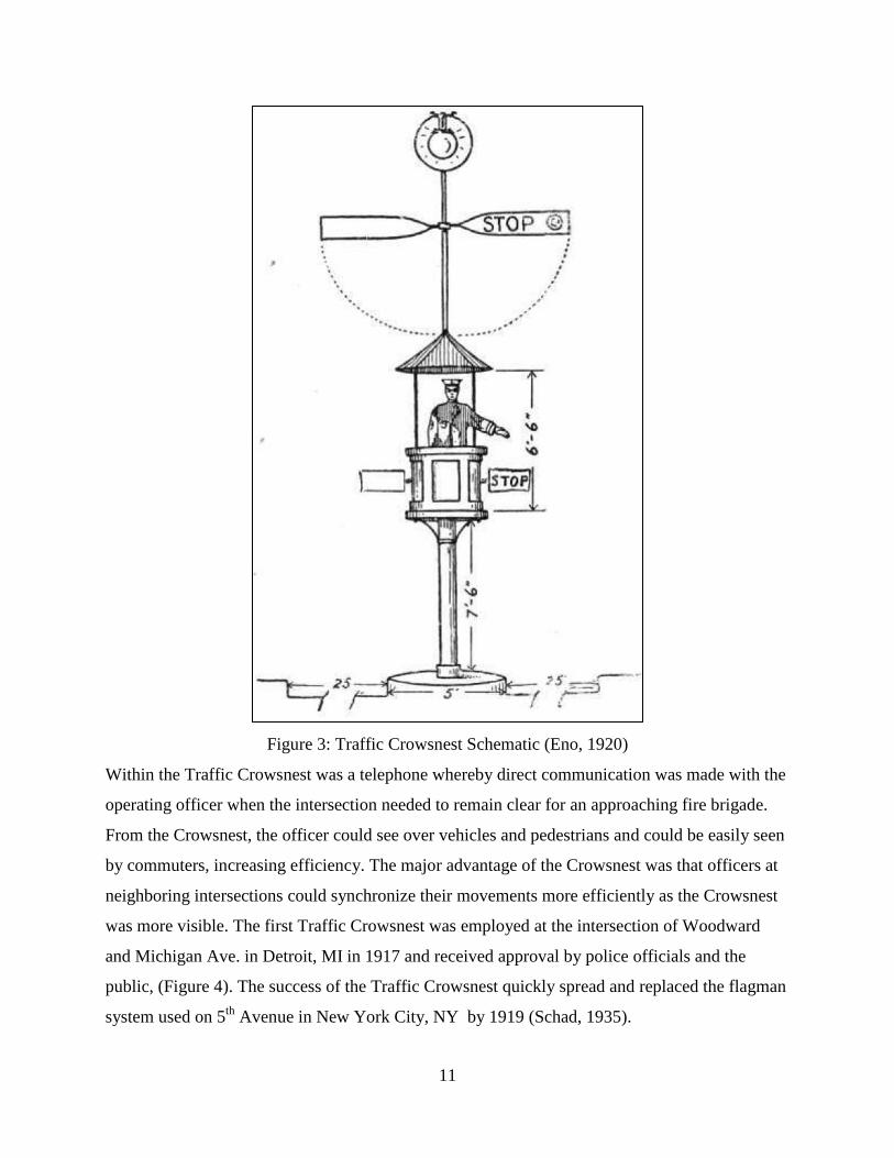
Figure 3: Traffic Crowsnest Schematic (Eno, 1920)

Within the Traffic Crowsnest was a telephone whereby direct communication was made with the

operating officer when the intersection needed to remain clear for an approaching fire brigade.

From the Crowsnest, the officer could see over vehicles and pedestrians and could be easily seen

by commuters, increasing efficiency. The major advantage of the Crowsnest was that officers at

neighboring intersections could synchronize their movements more efficiently as the Crowsnest

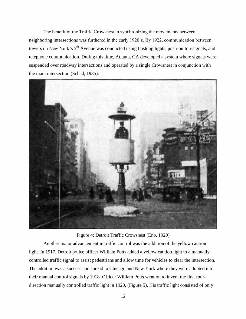
was more visible. The first Traffic Crowsnest was employed at the intersection of Woodward

and Michigan Ave. in Detroit, MI in 1917 and received approval by police officials and the

public, (Figure 4). The success of the Traffic Crowsnest quickly spread and replaced the flagman

system used on 5th

Avenue in New York City, NY by 1919 (Schad, 1935).

12

The benefit of the Traffic Crowsnest in synchronizing the movements between

neighboring intersections was furthered in the early 1920’s. By 1922, communication between

towers on New York’s 5th

Avenue was conducted using flashing lights, push-button-signals, and

telephone communication. During this time, Atlanta, GA developed a system where signals were

suspended over roadway intersections and operated by a single Crowsnest in conjunction with

the main intersection (Schad, 1935).

Figure 4: Detroit Traffic Crowsnest (Eno, 1920)

Another major advancement in traffic control was the addition of the yellow caution

light. In 1917, Detroit police officer William Potts added a yellow caution light to a manually

controlled traffic signal to assist pedestrians and allow time for vehicles to clear the intersection.

The addition was a success and spread to Chicago and New York where they were adopted into

their manual control signals by 1918. Officer William Potts went on to invent the first four-

direction manually controlled traffic light in 1920, (Figure 5). His traffic light consisted of only

13

three bulbs, requiring the location (top and bottom) of the red and green light to switch for each

approach. This light was state-of-the-art until the invention of the 12-bulb signal in 1928 (Lay,

1992).

Figure 5: Four Direction Three Bulb Traffic Light (Henry Ford Museum)

In 1922, the railroad signal company Crouse-Hinds developed the first automated timed

traffic signal (Halvorson, 1925). This signal controller was demonstrated on a nine-intersection

corridor in Houston, TX. The traffic signals were linked together and synchronized from a

central point. In 1923, Chicago deployed a similar system on Michigan Avenue spanning a

distance of 2.5 miles (Schad, 1935). By 1924, New York and Los Angeles had begun to adopt

the automated traffic signal controller. This system then spread rapidly through North America

and by the end of 1925, it was present in most major U.S. cities (Hoyt, 1927). By 1924, it was

estimated that one-thousand intersections in the U.S. were controlled by automated signal

controllers. This number grew to around 4000 by 1925 and 8000 by 1926, Figure 6.

Prior to the invention of the automated traffic signal, police had been the only

intersection traffic control measure used. With the widespread implementation of traffic control

systems, a debate emerged as to whether a police officer or an automated signal controller could

allocate intersection right-of-way more effectively. Burton Marsh, a traffic engineer for the

Pittsburgh Department of Public Safety summarized the advantages and disadvantages of police

control compared to automated timed control of intersections (Marsh, 1927). Marsh stated that

14

for a single isolated intersection, there was no better means of control then a police officer. He

contended that during an individual minute, an officer could outperform an automated signal

controller. He also stated that an officer had the ability to give priority to emergency and public

transportation vehicles, as well as allocate appropriate left turn movements (protected left turns

were not common circa 1927). Marsh summarized the advantages of manual traffic control as

“brain power efficiently used is, of course, usually better than mechanical control for a single

corner (intersection)”. Marsh also presented the disadvantages of manual control of isolated

intersection. His primary concern was that an officer had no way to coordinate his actions with

officers directing traffic at nearby intersections. He further contended that an officer at an

intersection was difficult to see by approaching vehicles and that, over time, an officer could

become complacent and distracted. Furthermore, the public sought to asked questions of the

officers, distracting them from their duties. Police officers, as one of their basic duties, must

write tickets and make arrests, which may take away from their traffic control responsibilities.

15

Figure 6: Estimate of Automated Traffic Signal Controllers in the U.S. (Marsh, 1927)

16

Another disadvantage of manual traffic control was the tendency toward human error. An officer

must be trained and experienced in directing traffic to become proficient; even veteran officers

can have bad days. The last and most pressing issue was the financial implication of manual

traffic control versus automated control. Marsh compared the operating cost of both control

strategies, stating that over the course of five years, an officer would operate an intersection for

eight hours a day at a cost of $9,200 (in 1927) as compared to an automated signal controller

which will cost $3,000 for 24 hour service, Table 2.

Table 2: Advantages and Disadvantages for Manual Traffic Control (Marsh, 1927)

Police Control of Isolated intersections

Advantages: Disadvantages:

An officer can control of an individual corner

better than any other means

An officer cannot coordinate his actions with

officers at neighboring intersections

An officer is best at allocating time

appropriately at any given instance

It can be difficult to see an officer standing a

the corner of the intersection

An officer can give priority to emergency and

public transportation vehicles An officer can become complacent over time

An officer can handle varying left hand turn

volumes better than any other signal control

system

An officer is subject to being asked questions

by the public

An officer can use common since judgments

at a moment notice An officer can be distracted easily

An officer must perform police duties

A rookie officer is subject to a learning curve

A veteran officer will have bad days on

occasion

An officer is much more expensive than an

automated signal controller

In addition to presenting the advantages and disadvantages of manual control, the article

presented the advantages and disadvantages of automated signal control. The article stated that

automated signal control was less expensive, easier to locate in an intersection, and could operate

24 hours a day independent of weather conditions. Additionally, automated signal control

reduced traffic accidents in the vicinity of an intersection, provided pedestrians a clear and

defined time to cross safely, and was more efficient at allocating green time at large or otherwise

complicated intersections. The disadvantages of automated signal control generally originated

17

from the fact a signal could not adjust to the current traffic volume. An automated signal

controller did not efficiently handle unbalance or widely-varying traffic volumes; the signal

allocated green time to movements which did not have demand and the signal was inefficient if

placed at intersections at which volume did not warrant them. Furthermore, automated signal

controllers were limited in the number of lights that could be used. Too many lights could

confuse drivers and the signal would require more frequent mechanical maintenance. The

advantages and disadvantages of automated traffic control are shown in Table 3.

Table 3: Advantages and Disadvantages for Automated Signal Control (Marsh, 1927)

Automated Signal Control of Isolated intersections

Advantages: Disadvantages:

A signal is less expensive than an officer A signal is limited in the number of lights it

can display

A signal is easier to locate and understand The time allotted each movement remains

constant throughout the day

Signals generally reduce traffic accidents in

the vicinity of an intersection

Signals have a hard time dealing with

unbalanced or widely varying traffic volumes

A signal gives pedestrian a clear and defined

time to cross

A signal requires regular mechanical

maintenance

A signal provides service 24 hours a day, 7

days a week

A signal at times will hold up traffic to allow

movements from the side streets, when there

is no demand for such movements

A signal is more efficient at allocating

intersection right-of-way for large or

otherwise complicated intersections

A signal will at times be placed at

intersections where traffic volumes do not

justify its placement.

The unmistakable advantage of automated traffic control was the cost over manual traffic

control. In 1928 New York City had an estimated 2,243 automated signal controllers (Hoyt,

1927). From the time period of 1925-1928 the New York City Police Department reduced its

traffic squad from 6,000 officers to 500 as a direct result of the added automated signal

controllers. This reduction in manpower resulted in a savings of $12,500,000 annually (Kane and

Finestone, 1928). This magnitude of savings was not restricted to New York City and

municipalities across the U.S. found they too could save millions by switching to automated

traffic signals. Traffic officials in Syracuse, NY claim that in addition to increasing travel times

in the central business district, the entire cost of implementing the new automated signal control

system was recovered in the first year by the savings made in officer salary (Walrath, 1925).

18

Additionally, automated traffic signals excelled were manual traffic control struggled; in

coordinating movements between neighboring intersections. Automated signals allowed

intersections within a corridor to be timed so that a driver could receive a green signal over the

entire span of the corridor. The coordinated signal control system was found to be more effective

than officers coordinating from traffic towers (Hoyt, 1927; Marsh, 1927). However, the

additional coordination was not without its drawbacks. It was found that drivers would race

down a coordinated corridor, attempting to keep up with the traffic signals (McShane, 1999). In a

traffic survey of Philadelphia (PA) in 1929, 341 automatically timed signal intersections under

coordinated control were evaluated for safety. The study found that collisions increased by 40

percent (Marsh, 1930). Marsh attributed the increase in accidents to poor implementation of the

traffic signals and not coordination.

The controversy over automated signal control was immediate with the spread of the new

systems implementation. Outspoken traffic research expert Miller McClintock believed that the

new signals would never replace police officers (McClintock, 1923). E. P. Goodrich, a consultant

engineer for the Borough of Manhattan dismissed automated signal control as a “fad” that would

pass and suggested the city not waste the money for their implementation (Goodrich, 1927).

William Philp Eno, considered to be the father of highway safety stated “students of traffic are

beginning to realize the false economy of mechanically controlled traffic, and hand work by

trained officers will again prevail” (Eno, 1927). The State of New Jersey required manual traffic

control for all state highways because officials believed automated signal control to be inefficient

for their truck-line highways (Marsh, 1927). Underlining these concerns was the belief that

without an officer present to enforce traffic laws at an intersection, drivers and pedestrians would

do as they please (McShane, 1999).

The push to overcome the obstacles faced by automated signal control came from the

engineering field. Based on the work done by early traffic engineers it was undeniable that

automated traffic control, as a means of general practice in urban environments was more

effective as a result of coordinated systems and more efficient financially, if by no other

measure. However, it was left to the engineering field to convince the commuting public. To do

this, engineering organizations collaborated with public and private representatives of the

motoring community. Furthermore, police agencies provided support to the movement to

automated signals by enforcing the first installments of the new system. The success of these

19

efforts is self-evident today. By 1930, semaphores, traffic towers and manual traffic control in

urban areas for routine traffic conditions was a thing of the past (Sessions, 1971). From this point

on automated traffic control was the dominate traffic control measure used in developed

countries.

After the 1920’s manual traffic control was reserved for directing special event and

emergency traffic. Conditions where routine traffic control plans do not adequately provide the

capacity needed for rare events. The previous research comparing manual traffic control to

automated traffic control only evaluates these strategies for routine conditions and not their

common practice today. The evaluation techniques used during this time (cura 1925) to compare

manual and automated signal control were qualitative in nature, not presenting any data on traffic

speed, travel time, volume, etc. Furthermore, advancements in both fields over the last 90 years

warrant a fresh comparison between the traffic control measures. There exists a gap in the

research that mandates a quantitative analysis between manual traffic control and modern signal

controllers for use during planned special events and emergencies.

2.2 Manual of Uniform Traffic Control Devices (MUTCD)

The Manual of Uniform Traffic Control Devices (MUTCD) is the document that sets the

national standards for all traffic control devices governing streets, highways, bikeways and

roadways otherwise open to public travel in the United States. The MUTCD designates a traffic

control device as any signs, signal, markings or any other devise used to regulate, warn or guide

motor vehicles, bicyclist or pedestrians (MUTCD, 2009). Prior to the publication of the first

MUTCD in 1935, two previous manuals governed traffic control devices in the U.S. (Hawkins,

1992). The first published in 1927 then revised in 1929 was the Manual and Specifications for

the Manufacture, Display and Erection of U.S. Standard Road Markers and Signs. This

document was sponsored by the American Association of State Highway Officials (AASHO) in

conjunction with the National Conference on Street and Highways Safety (NCSHS). AASHO is

now known as the American Association of State Highway Transportation Officials (AASHTO).

This manual provided standards for rural roads and did not include standards for traffic signals;

manual, automatic or otherwise (AASHO, 1929). The other predecessor to the MUTCD was the

Manual on Street Traffic Signs, Signal and Markings, also sponsored by the National Conference

on Street and Highway Safety (NCSHS). This manual, in contrast to the Manual and

Specifications for the Manufacture, Display and Erection of U.S. Standard Road Markers and

20

Signs, was designed to accommodate urban traffic signs, markings and was the first national

standard for traffic signal regulation in the U.S. However, having two set of national regulations

governing roadway sign, signals and markings was undesirable. Therefore, the MUTCD was

created to bring uniformity and establish a single source for regulating the design of road sign,

signals and markings (MUTCD, 2009).

The National Conference on Street and Highway Safety was responsible for the Manual

on Street Traffic Signs, Signal and Markings. This document makes no mention of manual traffic

control but does note “Traffic officers stationed in roadways shall be illuminated at night, by

flood lights if necessary, in the interest of safety” (NCSHS, 1930a). However the NCSHS, in an

attempt to bring uniformity to city traffic laws published a model set of municipal traffic

ordinances. In this document, the authors recognize the role of police and the need for their

authority in directing traffic.

It shall be the duty of the Police Department of this city to enforce the provisions of this

ordinance. Officers of the Police Department are hereby authorized to direct all traffic

either in person or by means of visible or audible signal in conformance with the

provisions of this Ordinance, provided that in the event of a fire or other emergency or to

expedite traffic or safeguard pedestrians, officers of the Police or Fire Department may

direct traffic, as conditions may require, notwithstanding the provision of this Ordinance

(NCSHS, 1930b).

The most recent MUTCD published in 2009 makes little mention of manual traffic

control of intersections. The document discusses traffic incidents and states, “if manual traffic

control is needed it should be provided by qualified flaggers or uniformed law enforcement”

(MUTCD, 2009). The manual does however specify that officers directing traffic are subject to

the same high-visibility safety apparel as flagmen when operating near the roadway.

Furthermore, the MUTCD developed a Traffic Control Point Sign (EM-3) to be used at locations

where manual traffic control is used on a regular basis (MUTCD, 2009). Other than these three

instances, the 862 page document publishing the national standards for all traffic control makes

no mention of manual traffic control despite its frequent use during planned special events and

emergencies.

21

2.3 Police Training For Traffic Control

The effectiveness of a police officer at directing traffic is a function of training and

experience. Prior to formal regulations, officer training was conducted entirely within each

department. Specialized training for law enforcement officers first emerged in 1935 with the

founding of the FBI National Academy (Hoover, 1947). Between the years of 1935 and 1944 the

FBI National Academy sent instructors to 1,513 local, county and state police agencies. In 1946

alone the academy instructed 1,785 schools attended by almost 90,000 law enforcement officials.

Due to the size and scope of the traffic problem the FBI national Academy included traffic

training from its founding in 1935 (Hoover, 1950). As director of the Federal Bureau of

Investigations (FBI), J. Edgar Hoover institutionalized uniform training programs and training

templates for police traffic control. Hoover believed that “the development of police executives

and instructors cannot be accomplished without adequate training in traffic law enforcement”

(Hoover, 1950). The FBI made police traffic control training available to local law enforcement

in urban and rural areas. In 1949 over 150 police training schools were held specializing in

traffic control. Small stations which did not have an adequate number of officers to justify

holding an entire course at their department could go to “Zone Schools” which allowed officers

from many neighboring communities to attend (Hoover, 1947; Hoover, 1950).

2.3.1 Northwestern University Traffic Institute

Private traffic control training for law enforcement officers began in 1936 with the

founding of the Traffic Safety Institute at Northwestern University (Bradford, 2013). The Traffic

Safety Institute, later known as the Traffic Institute, trained officers in crash prevention, traffic

supervision and police management. Traffic supervision had three direct functions, accident

investigation, traffic law enforcement and traffic direction (Woods, 1952). Since the founding of

the Traffic Institute it has published several documents on manual traffic control.

Police traffic direction is defined by the Northwestern University Traffic Institute (NUTI)

as “telling drivers and pedestrians how and where they may or may not move or stand at a

particular place, especially during periods of congestion or in emergencies” (Woods, 1952).

Published in 1952 the article Directing Traffic, what it is and what it does, was the first of its

kind in providing a cross-jurisdictional standard for manual traffic control. While manual control

had become more-or-less standardized in practice, this article was the first to publish and

disseminate the procedure. The article states that officers while directing traffic must answer

22

inquiries, tell drivers and pedestrians what to do and what not to do and in the cases of

emergency traffic control, make rules for the flow of traffic when usual rules are inadequate. The

article tells officers to act as a traffic light operating in coordination with neighboring signals,

never allowing more vehicles through the intersection which the downstream intersection cannot

handle (Woods, 1952). However, the article does not provide guidance on how to effectively and

efficiently direct traffic in practice.

In 1960, the NUTI put out the first edition of Signals and Gestures for Directing Traffic.

This publication was revised five times; the most recent version was released in 1986. The article

explained, through illustration, how a police officer should communicate with vehicles and

pedestrians while directing traffic. First, it explained different postures and then went on to

illustrate how each hand gesture corresponded to a vehicle movement or action. The article then

moved on to controlling traffic using the “clicker” method, however, the article implied that the

“officer in the intersection” approach was more effective at directing traffic. Finally, the article

concluded by explaining the role of the baton and whistle, as well as how to cope with directing

traffic at night (NUTI, 1986). The article may be a good instructional guide for communications

while directing traffic, but does not lend any insight on how to effectively or efficiently direct

traffic.

The follow-up publication of NUTI to Signals and Gestures for Directing Traffic was

Directing Vehicle Movements, published in 1961. This article was unique in that it employed

traffic engineering concepts to assist in the effectiveness of manual traffic control. The guide

stated that manual control is only necessary when an intersection is oversaturated for its current

control technique (e.g., signal control, stop controlled, priority controlled), citing that motorists

will exercise undue caution when entering an intersection governed by a police officer in the

same fashion that drivers will hesitate to overtake a police patrol vehicle while driving on the

highway. The presence of an officer inevitably led to a loss of efficiency and, thus, an officer

should only direct traffic in situations where manual traffic control will offset the initial loss in

efficiency. Therefore, an officer was only able to direct traffic when needed in oversaturated

conditions. The article instructed officers to equitably distribute delay time between movements

based on volume. Delaying one car for 30-seconds is equivalent to delaying 30 cars for one

second, as such low volume movements should be delayed for longer periods. To maximize

saturation flow rate, officers were instructed to hold a movement’s initial arrival until a group of

23

vehicles formed, and then switch to that direction and keep them there so long as vehicles depart

one right after the next. It stated officers should not keep vehicles waiting for longer than a

minute in the hope of collecting a group and officers should not prolong green time for a single

vehicle. The article stresses the importance of preventing queues from propagating into

neighboring intersections. It instructed officers to force vehicles to detour if the queue is

threating the upstream intersection. At an intersection where cross-street traffic and main-street

traffic were equal, the officers were told to increase cycle length to reduce start-up lost-time and

increase effective green time. Also, it stated officers should never waste green time; if an exit

lane was blocked, officers were told to immediately switch to a free-flowing movement until

adequate room was provide to allow the previously-blocked movement to continue. When

switching between movements, officers were informed to wait until a natural gap in the traffic

stream appeared. If no gap existed, officers were instructed to stop the flow of vehicles after a

heavy truck. By letting the heavy truck pass the intersection, the start-up lost-time of having to

halt and restart the large vehicle was reduced. In addition to informing officers on how to

increase efficiency, officers were instructed on how to improve safety. Officers are told where to

stand in the intersection, how to cope with wet and icy environments, and how to remain safe in

intersections with irregular geometries (NUTI, 1961). The article assumed that the “officer in the

intersection” approach was more efficient then the “clicker” method, which may not be true

today given the advancements in traffic signal controllers.

2.3.2 Modern Police Training for Traffic Control

In 1973 the International Association of Chiefs of Police (IACP) collaborated with the

National Highway Traffic Safety Administration (NHTSA) to develop a comprehensive

collection of police traffic service polices for best practice. This partnership developed the Police

Traffic Service Basic Training Program (Hale and Hamilton, 1973). The goal of this program

was to improve the effectiveness of the National Highway Safety Program by establishing

national standards on jurisdictional law enforcement training to provide police officers with

basic, uniform training in police traffic services. This national training program was targeted at

six major areas; 1) policy and traffic service, 2) traffic law, 3) traffic direction and control, 4)

traffic law enforcement, 5) traffic management, and 6) traffic court. The traffic direction and

control section of the training program stated that an officer had three goals when directing

traffic: safe movement of vehicles and pedestrians, the mitigation of traffic congestion, and

24

ensuring driver comply with traffic laws. The training program also discussed instances where

police traffic control should be used, areas of periodic congestion (e.g., rush hour choke points),

special events, and around hazardous scenes. However, the training program did not include

guidance in determining when it may be more beneficial to use police in lieu of signalized

control, when it should be used, where it can best be implemented, or how to evaluate its effect

on the overall movement of traffic during emergencies, events, or routine traffic conditions.

By 1977, the IACP and NHTSA partnership had developed a system for evaluating police

traffic services for the nation. This guide was intended to assist police agencies in determining

the quantity and quality of services provided by their traffic control division. The manual was

designed to evaluate an individual police officer’s performance. It was possible to measure and

evaluate the performance of traffic control for a department if aggregated for the entire police

force. The manual evaluated an officer based on several factors related to traffic control. An

officer’s performance while directing traffic was based on the traffic flow through the

intersection and eye witness reports of the officer’s actions (NHTSA, 1977).

In 1986, the IACP and NHTSA published the Manual of Model Police Traffic Services

Policies and Procedures. This document consolidated, revised, and updated the work done in the

previous decade. This effort was motivated by the need for police officials to remain compliant

with traffic-related standards set by the Commission on Accreditation for Law Enforcement

Agencies. The document detailed traffic control functions, such as staff and administrative

service, traffic law enforcement, accident management, traffic direction and control, traffic

engineering and ancillary motorist services. Under traffic direction and control, the document

provided guidance on general policy and procedure, as well as identifying locations for traffic

control, implementing temporary traffic control devices and traffic direction for special events,

fire scenes, and adverse road conditions (NHTSA, 1986). An important note here was that only

the policy differs with regard to directing traffic for regular operations, special events, and fire

scene—not the procedure. The procedure for directing traffic remained the same regardless of

the application.

Over the years, numerous other manuals were developed to describe the proper

functioning of police traffic control (Leonard, 1973; Weston, 1996). However, these documents

focus primarily on the role of police in accident reduction, selective traffic law enforcement, and

the development of a traffic-orientated police force. They also provided guidelines for officer

25

safety by identifying where and how to move within a congested intersection. The book by

Weston (1996) provided a comprehensive reference for ensuring safety while directing traffic,

but it did not specify when it may be more beneficial to use police in lieu of signalized control,

when it should be used, where it can best be implemented, or how to evaluate its effect on the

overall movement of traffic during emergencies, events, or routine traffic conditions.

2.4 Technical Manuals, Handbooks and Published Guidelines

An extensive amount of unpublished or otherwise not widely-disseminated practitioner

training references exist for manual traffic control. These manuals have generally addressed the

“nuts and bolts” of traffic direction. In general, they are designed to be a quick reference for an

individual new to manual traffic control. These documents were usually developed by individual

police departments and used as a jurisdictional guideline for new police officers. Most of these

manuals were not made to be cited references and as such many do not list an author or date of

publication. These documents were for “in-house” use, authored by senior officers on the force

with years of manual traffic control experience.

Despite being developed to meet local traffic control needs, these manuals showed

consistency with references to several key points. All of the reviewed documents shared the

following:

The use of reflective vest at all times

The use of lighting for directing traffic in adverse weather

The need for additional lighting at night from the police vehicle or additional flood lights

Where to stand within the intersection

How the officer should position his/her body to command vehicles

Uniform hand signals to start and stop the flow of traffic

Safety when directing conflicting turn movements

The use of traffic control tools such as flashlights, whistle, illuminated batons and flares

While consistent, these documents have been inadequate in providing guidance on how to

effectively distribute intersection right-of-way. These documents provided a “how to” for

directing traffic; after reading one of these manuals an officer would know “how to” start and

stop the flow of vehicles but would not know when or why. Without a basic understanding of

traffic engineering concepts behind intersection control, which police officers developed with

experience, new officers would certainly perform poorly. (Florida Highway Patrol, 1996;

26

Houston Police Department, 2004; Shults, 2005; Epperson, 2006; Jones, 2008; Anne Arundel

County Police Department, 2009; Lincoln Police Department, 2011; Lundborn, 2011; Burlington

Police Department, xxxx; City of Los Angeles Personnel Department, xxxx; Johnson, xxxx).

2.5 Special Event and Emergency Planning

Nearly every major planned special event has had a traffic management plan.

Furthermore, most municipalities have had an emergency operations or emergency evacuation

plan on some level (Region, State, County, City, etc.). Traffic management plans for special

events and emergencies have been developed based on a set of common guidelines. For an

emergency evacuation plan, the guidelines consisted of government regulations that typically

required planning action. For planned special events, the guidelines were more of a collection of

best practices aimed at assisting municipalities in event planning and management. Instead of

looking at individual publications of traffic management plans, this sections looked at the

guidelines by which authorities developing these plans use for guidance.

2.5.1 Special Event Planning

The National Cooperative Highway Research Program (NCHRP) had a mission to

collect, evaluate and disseminate information on common highway problems faced by highway

administrators, engineers and researchers. The synthesis series presented the state-of-the-practice

in how these everyday problems were solved around the nation. One such problem,

transportation planning and management for special events was addressed by NCHRP Synthesis

309. The document presented the ways by which agencies plan, coordinate, and manage the

transportation system for planned special events. This document was a compendium of the best

knowledge available on the practice of special event traffic management planning. When

developing a traffic management plan for a special event, the “go to” document is the NCHRP

309.

The NCHRP synthesis 309 addressed all aspects of highway management for planned

special events. This document made frequent reference to the use of police officers for manned

traffic control points. “The advantage of using staffed traffic posts over signalized control is the

presence of authority and the ability to make dynamic changes to the traffic flow”. Based on the

survey conducted in NCHRP 309, manual traffic control of intersections for special events was a

common traffic management technique used around the country. Therefore, any agency looking

to develop a special event traffic management plan was encouraged to use manual traffic control.

27

Furthermore, these agencies were encouraged to use traffic simulation in the development of

management plans. However, any event utilizing manual traffic control currently would have no

reliable way of simulating the process for a comparative analysis.

2.5.2 Emergency Planning

Emergency planning has been governed by the Federal Emergency Response Agency

(FEMA) and the Department of Homeland Security (DHS). These two departments, in a joint

effort, developed the National Response Framework (NRF). The NRF was designed to assist

personnel, governmental, commercial, and non-governmental organization officials in the

response and recovery needed from a major disaster. The NRF developed various documents to

assist state and local governments to create emergency traffic management plans for an all-

hazards emergency (FEMA, 2009). One such set of documents, the Emergency Support Function

(ESF), provided the structure for coordinating the interagency support needed to obtain federal

resources to assist in the response to an emergency incident. The roles and responsibilities of

relevant stakeholders are defined in a series of 15 documents known as the ESF Annexes. In

order to obtain federal support in response to a disaster, the state and local government must

comply with NRF and the ESF Annexes (FEMA, 2013).

The Emergency Support Function #13, Public Safety and Security Annex, provides

federal assistance to local and state governments in order to maintain safety and security. Within

this annex, the federal government may provide assistance to the local agencies for traffic control

operations, namely traffic direction and control for vehicles and large crowds (ESF#13, 2009).

The Mass Evacuation Incident Annex provides the criteria needed for federal support to assist in

a mass evacuation. This annex stated that local police should be used to control the flow of

vehicles on federal and state routes. This document referenced ESF #13 for the administration of

traffic direction and control.

While FEMA and DHS have been the authoritative sources for the development of

emergency traffic management plans for natural and man-made disasters, the traffic management

plans for evacuations from nuclear power plant failures has been governed by the United States

Nuclear Regulatory Commission (NRC). The NRC mandates, through governmental regulation,

evacuation time estimates be developed for the population within the area surrounding a nuclear

power plant (NRC, 1980). An evacuation time estimate (ETE) has been the calculated time

required to evacuate an evacuation planning zone located within a ten mile radius of a nuclear

28

power plant. The ETE has been primarily used by decision-makers to assist in choosing the

correct protective action in the event of an incident at a nuclear power plant. However, it may

also be used in the development of traffic management plans to support an evacuation (NRC,

2011).

The criteria for developing an ETE were given by NUREG/CR-7002 Criteria for

Development of Evacuation Times Estimate Studies. This document highlighted manual traffic

control stating, “In general, it may be assumed that manned traffic controlled intersections

operate most efficiently” when compared to un-signalized, fixed-time signals and actuated

signals. This document also supported the use of traffic simulation in the development of ETEs.

It mandated that if manual traffic control is proposed as a part of a traffic management plan, then

the simulation model must simulate the effects of manual traffic control. The document proposed

modeling manual traffic control as an actuated signal with a signal timing plan which reflected

more efficient operations (NRC, 2011). However, without full knowledge of manual traffic

control operations, simulating manual traffic control as an actuated signal may not be realistic.

Furthermore, no guidance was given on how to make the simulated actuated signal more

efficient or how to simulate the actuated signal to produce results similar to that of manual traffic

control.

2.6 Manual Traffic Control and Empirical Studies

Since the first studies to evaluate the effectiveness of manual traffic control in the 1920’s

relatively little work has been conducted on this form of control. Since the 1920’s, manual traffic

control under routine conditions in urban intersections was no longer commonplace (Sessions,

1971). After this time, manual traffic control has been primarily used for special events and

emergency situations. However, in rare situations, manual traffic control is still used to

supplement automated traffic controllers during peak hour periods in urban and rural areas. This

was the case in Fort Belvoir, Virginia in 1953. At that time, a traffic study of ten intersections

with narrow-width approaches (total width of two-way streets is less than thirty feet) was

conducted to determine if the approach widths needed to be expanded (Sutermeister, 1956). Of

the ten intersections studied, six were manually controlled by police officers (some using the

“stand in the intersection” method and others using the “clicker” method), two were controlled

under fixed time settings, one was an actuated controller, and the final one was all-way stop

controlled. The highest capacities were observed using manual traffic control strategies. This was

29

accomplished by officers extending the green time to the priority approach at the cost of the

cross-street traffic. The report stated that during the 15-minute peak period, 31 approaches where

found to be overloaded, however only two were recommended for widening. The study

suggested that this was due to the added capacity of manual traffic control at the intersection and

thus widening of the approach lanes was not necessary. Unfortunately, the study did not

discriminate between manual traffic control conducted by the “officer in the intersection”

approach or the “clicker” approach. This would have allowed more insight into the operational

advantages of manual traffic control.

A study conducted in Brisbane, Australia evaluated manual traffic control to supplement

congested at an un-signalized priority-controlled intersection during peak periods. As a part of

this research a priority-controlled intersection was analyzed under manual traffic control during

the evening peak period. From the rooftop of a nearby building, researchers used stopwatches to

observe and time an officer directing traffic. The researchers recorded parameters such as phase

length, number of vehicles and type, maximum queue length and the time to clear each queue.

These values were then used to compare the officer’s performance to a hypothetical pre-timed

and actuated traffic controller. The study found that saturation flow rate was not effected by

manual control but average approach delay was slightly lower than expected when compared to a

pre-timed isolated intersection. The paper concluded that it was unable to prove that an officer

was superior to a traffic signal (Pretty, 1973). However, this conclusion is not generalizable

based on the evidence that the study only considered one intersection under police control and

observed this intersection for only one hour. Furthermore, the article states that the intersection

was under-saturated. One of the primary applications for manual traffic control is for special

events and emergency traffic, almost certainly operating in oversaturated conditions.

In some developing countries with high levels of congestion, manual traffic control

during peak periods remains common for critical intersections. May and Montgomery (1988)

evaluated pre-timed signal control settings as an alternative to manual traffic control for isolated

and linked intersections in Bangkok, Thailand. An isolated intersection was studied for six days

during evening peak periods. On days one, three, and five of the study pre-timed signalized

control was used at the intersection. On days two, four, and six manual “clicker” control was

used. Over the course of the experiment, the pre-timed signal control cycle and phase length

settings were adjusted to increase their effectiveness. The results showed that at isolated

30

intersections with over-saturated conditions, police out-performed pre-timed signal control on

the basis of delay, queue length, and total throughput. The authors noted that saturation flow rate

decreased over time, which represented inefficiencies in manual control as a result of long phase

lengths.

This research also applied the same experimental methodology to evaluate the

performance of pre-timed signal control at four linked intersections as a replacement to manual

control. The study evaluated the four pre-timed signal settings over five consecutive days and

compared the results of manual control to the following four days (excluding Saturday and

Sunday). The results showed that a 21 percent decrease in travel time and a 29 percent increase

in travel speed were possible using pre-timed coordinated signals as opposed to manual traffic

control. However, it was necessary to have manual intervention when the corridor capacity was

effected by major traffic incidents. The conclusions of this research were also backed by a

quantitative analysis but, based on the high variation of the traffic demand between observation-

days, the small sample size was not sufficient to draw statistically confident conclusion.

Another comparison of manual traffic control and automated control was conducted in

Israel (Mahalel, Gur and Shiftan, 1991). This research compared manual traffic control of two

isolated intersections to control by an actuated signal in oversaturated conditions. The first

intersection was observed for two days under actuated signal control and four days under manual

control. The second intersection was observed for one day of each. It was found that in over-

saturated conditions, the actuated control performed similar to a pre-timed setting due to the

recall of the maximum green. The research used total throughput and degree of saturation as

measures of effectiveness. The study results showed that manual control was correlated to a

decrease in lost-time by as much as 60 percent and an effective green time increase of 15%. This

reduction in lost-time was attributed to the use of the longer cycles associated with manual

control, resulting in fewer cycles per hour.

Confirming the findings found by May and Montgomery (1988), the Israeli research

study also identified a decrease in saturation flow rate as phase length increased, despite the

persistence of long queues. The authors quantified this phenomenon showing that 55 seconds

into the phase, saturation flow rate decreased rapidly. This observation suggested that a trade-off

exists between long phase length (increases in effective green time) and efficient use of green

time (decreasing saturation flow rate). Further analyses of intersection throughput found that

31

manual traffic control increased intersection capacity by as much as 9 percent, confirming the

result found by Sutermeister (1956). A comparison of the degree of saturation suggested that

manual control could increase capacity to such an extent that it could surpass demand. This

conclusion is based on a comparison assuming constant cycle length and green splits for manual

control. Research conducted by Marsh (1927) found that officers directing traffic do not operate

in this manner. Furthermore, many of the advantages of manual traffic control can be hindered

by such assumptions (see Table 2). Therefore, conclusion suggested by Mahalel, Gur and

Shiftan, (1991) are confirmed by previous research but due to the stated assumptions the

magnitude of the capacity increase caused by manual traffic control may be larger. With a

simulation tool for manual control these assumptions would not have been necessary.

During peak hours, roundabout intersections may also be supplemented with police

control if demand warrants. A comparison of a police controlled roundabout to a traditional four-

leg intersection evaluated intersection performance with regard to dynamic delay (i.e., delay

from the end of a moving queue) was undertaken by Al-Madani (2002). Selecting two

intersections (one roundabout and one traditional signalized four-leg) with similar traffic and

geometric characteristics, video detection was used to produce vehicle trajectories. From these

trajectories, vehicle delay was plotted against queue length for both intersections. The results

showed that at distances less than 262ft (80m), the police controlled roundabout significantly out

preformed the four-leg signalized intersection. However, when queue length surpassed this

threshold, the four-leg signalized intersection reduced delay considerably when compared to the

police controlled roundabout. It is uncertain whether the cause of this phenomenon could be

attributed to the police control or the effect of an over-congested roundabout. Given the small

sample size, the conclusions of this paper may not be widely generalizable to other locations and

sets of conditions.

Manual traffic control has also been used frequently at all-way-stop controlled

intersections before and after special events. Traffic volume at these intersections typically does

not justify installing a traffic signal but during these instances of high, non-recurring congestion,

manual traffic control is used to assist intersection operations. Using traffic simulation modeling,

a comparison of manual traffic control and pre-timed signal control of an all-way-stop controlled

intersection during a special event was undertaken by Ye, Veneziano and Lassacher (2008). This

research determined the saturation flow rate from a one and half hour video recording of manual

32

control operations. The saturation flow rate at this location was estimated to be 1,300 vehicles

per hour. This is considerably less than the results of an earlier study by Pretty (1973) where the

saturation flow rate was found to be nearly 1,700 vehicles per hour per lane.

During the observation period Ye, Veneziano and Lassacher (2008) observed the

saturation flow rate decrease overtime; confirming the findings of Mahalel, Gur and Shiftan

(1991) and May and Montgomery (1988) though not to the same extent. The manually controlled

intersection was simulated as a pre-timed signal control using average cycle and phase lengths

observed during the peak period of the special event traffic. These results were then compared to

an optimized pre-timed signal plan within a traffic simulation environment. The results of the

simulation showed that the optimized signal plan reduced vehicle delay by over half when

compared to manual control. However, to simulate manual traffic control, this research assumed

constant cycle lengths and phase splits in the same fashion as Mahalel, Gur and Shiftan, (1991)

and contradicting Marsh (1927).

2.7 Summary of Literature Review Findings

Previous research on manual traffic control has shown that in oversaturated conditions, it

outperforms automated control for isolated intersections (Sutermeister, 1953; May and

Montongomery, 1988; Mahalel, Gur and Shiftan, 1991). However, in the case of under-saturated

intersections, automated control prevails (Petty, 1974; Ye, Venexiano and Lassacher, 2008).

Research conducted before the 1930’s found that automated signal control outperformed

manual control for coordinated systems (Marsh, 1927; Hoyt, 1927; Marsh 1930). Similar results

were shown using a quantitative approach in more recent research (May and Montgomery,

1988). They also showed previous research agrees that under manual control, saturation flow rate

decreases overtime as phase lengths increase (May and Montogomery, 1988; Mahalel, Gur and

Shiftan, 1991; Ye, Venexiano and Lassacher, 2008). However, research on manual traffic control

has been generally based on small sample sizes leading to questionable conclusions based on

implied statistical significance. Furthermore, the previous research has only investigated the

officer’s effect on the traffic stream and not what events in the traffic stream effect the officer’s

decision making. Studies attempting to simulate manual traffic control have done so by assuming

officers act like traffic lights, with constant cycle lengths and phase splits (Pretty, 1973; Mahalel,

Gur and Shiftan, 1991; Ye, Venexiano and Lassacher, 2008). However, the emerpical

observations show this is not the casue. Furthermore, Marsh (1927) suggested that many of the

33

advantages of manual traffic control come from not having constant cycle length and phase

splits. A comparison of Table 2 and Table 3 showed that the advantages of manual traffic control

have been in an officer’s ability to extend green time when needed, cut short phase, and

accommodate unbalanced and uneven traffic volumes (Marsh, 1927; Eno, 1927; Schad, 1935).

Oversimplifying manual traffic in simulation models by assuming constant cycle length and

phase splits could lead to an unfair comparison between manual traffic control and automated

control.

The most important conclusion of the review of past research studies and other

documents showed that there is a gap in the base of knowledge, in there have been no studies

using a statistically significant sample size to evaluated manual traffic control for planned special

event and emergencies. At present, no research has been conducted on the stimulus-response

relationship between the traffic stream and officer decision making while directing traffic. Also

no research to date has ever programmed the traffic light to act as an officer, having phase length

dictated by stimuli in the traffic stream. The research proposed in this report seeks to fill the gaps

in knowledge by developing a discrete choice model able to replicate the actions taken by a

police officer while directing traffic. The discrete choice model will then be programed into a

traffic simulation model to replicate the police officer’s logic while directing traffic. By

incorporating the discrete choice model into the simulation model, the oversimplification and

broad assumption made by Pretty (1973), Mahalel, Gur and Shiftan (1991) and Ye, Venexiano

and Lassacher (2008) are not required, allowing for an “apples to apples” comparison of manual

traffic control and automated control. The methodology used to undertake the work necessary to

achieve these objectives is described in the following chapter.

34

35

CHAPTER 3. METHODOLOGY

The research methodology was developed to analyze and model manual traffic control.

The methodology addresses the gaps in literature described in the second chapter. Broadly, the

research methodology consisted of four primary tasks. The first task was the collection and

processing of video footage of police officers directing traffic. The second task was the

development of a discrete choice model capable of explaining right-of-way allocation decisions

made by the police officers. The third task was programing the discrete choice model into the

microscopic traffic simulator, VISSIM 5.3, to simulate the police officer directing traffic by

“replacing” the intersection signal controller logic. The final task was to use this model to

compare simulated manual traffic control model to a fully actuated signal controller.

Figure 7 provides a flowchart that graphically represents this methodology. The

following sections of this chapter describe the primary research task: Data Collection and

Reduction, Discrete Choice Modeling, and Simulation Model Development.

3.1 Data Collection and Reduction

The data requirements for discrete choice modeling dictated an extensive collection

effort. Data was collected from nine intersections for eight special events in Baton Rouge, LA

and Miami Gardens, FL. The data collection effort spanned over four months starting in the Fall

2012. In total, video data from over 320 hours of special event traffic was collected, viewed and

cataloged. This was necessary because the location and timing of where and when police officers

would direct traffic was unknown. From this video footage collected a total of 26 hours and 27

minutes (less than 10% of the total footage collected) was of police officers actively directing

traffic.

36

Figure 7: Methodology Flow Chart

Data Reduction

Discrete Choice Model Simulation Model V.A.P.

Output Parameters

Data Collection

Videos

Do the output

parameters match the

data collection videos?

Comparative Analysis

Statistical Results

NO NO

YES

37

In Baton Rouge, LA five intersections were selected for data collection during four

special events. These intersections were selected from the LSU Game Day Traffic Management

Plan provided by the Baton Rouge Department of Public Works. Of the five intersections

selected in Baton Rouge, only three were observed to have police officers direct traffic in the

video database. These intersections were Stanford and Perkins, Nicholson and Roosevelt and

Nicholson and Lee. Their location in reference to Tiger Stadium at the LSU campus can be seen

in Figure 8. The intersection of Nicholson and Lee is in close proximity (within 30 ft.) of a

railroad crossing which, is not shown in the figure. The geometric configuration of the study

intersection is provided in Appendix A.

In Miami Gardens, FL cameras were placed at four major intersection surrounding Sun

Life Stadium for four special events. These intersections were chosen because of their proximity

to the stadium and their location on critical routes. Of these four intersections one was observed

to be under police control in the video database and for only three of the four events (one of the

events did not use manual traffic control at any intersection). The study intersection located in

Miami Gardens, FL was NW 183 St. and NW 27 Ave. Its location in reference to Sun Life

Stadium is shown in Figure 9. The geometric design of this intersection is also provided in

Appendix A.

Data for this study was collected from special event traffic only. While it would have

been preferable to collect data from a mix of both special event and emergency situations, it was

not practical with the scope and time schedule of the research. This research makes a broad

assumption that manual traffic control is likely to be conducted similarly for special events and

emergencies. The literature review provided justification for this assumption in modern police

training (NHTSA, 1986) even though this research did not independently verify this.

38

Figure 8: Baton Rouge, LA Study Area

39

Figure 9: Miami Gardens, FL Study Area

Video recording was the preferred method to collect data because it was relatively

inexpensive when compared to the labor cost associated with alternative methods. The video

recording also allowed for a permanent record of the events and was the preferred data collection

method in previous research (Al-Madani, 2002; Ye, Veneziano and Lassacher, 2008).

The data used in this research is summarized in Table 4. The remainder of this section

describes how the video data was collected and processed for the development of the discrete

40

choice and simulation models. The study events, collection equipment, pricing, and camera

positioning within the intersection are also detailed. This section concludes with a description of

the qualitative observations made during the video processing.

Table 4: Data Collection

Event Time Location

Num.

Events

Num.

Intersections

Num.

Obs.

Time of Manual Control

(Hours: Minutes)

Fall 2012 Baton Rouge 4 3 12 21:49

Winter 2012 Miami Gardens 3 1 3 4:38

Total 7 4 15 26:27

3.1.1 Data Collection Device

The initial task required to collect the data was to identify a camera that satisfied the data

collection requirements. The camera needed to record for at least four hours, provide high

definition video quality and be waterproof. Also, it was desirable to have a camera that was

securable and inexpensive. Based on these requirements the GoPro HD HERO™ was selected as

the data collection camera.

The GoPro HD HERO™ is designed to be mounted on sporting equipment (helmets, dirt

bikes, surfboards, etc.). It also records in HD and is waterproof. With an upgraded battery add-on

and additional hard drive the camera can record for over five hours. While the camera is not

securable, its small size made it easy to deploy and collect in the same day. Furthermore, the

camera’s discrete profile made it go unnoticed among the existing intersection equipment

(pedestrian call box, signal cables, detecting equipment, etc.). Figure 10 shows the entire video

data collection assembly including GoPro HD HERO™, the Battery BacPac™, GoPro LCD

Touch™ viewing screen, the waterproof case, plastic mounting platform, and 32 GB memory

card used in each camera. The major advantage of the GoPro when compared to other camera

alternatives was that the camera, power source and hard drive were self-contained in a small

waterproof case. In wide angle mode the camera was capable of capturing a nearly 180° field of

vision. This meant that only two cameras were required at each intersection to capture the

approach queue length.

Ten sets of this camera assembly were purchased for a total cost of approximately $2,230

plus tax and shipping. Table 5 details these expenses.

41

Table 5: Data Collection Equipment Cost (US Dollars)

Description: Price: Quantity: Cost:

GoPro HD HERO Camera $129.99 10 $1,299.90

Battery BacPac $49.99 10 $499.90

SanDisk 32GB SD Class 4 Card $34.99 10 $349.90

GoPro LCD Touch BacPac $79.99 1 $79.99

Tax

$89.19

Total

$2,318.88

The cameras were mounted to the traffic signal strain poles of each intersection. A

camera was placed on the pole diagonally across from the traffic control box of each intersection

while another camera was placed on the strain pole above the traffic control box, Figure 11.

These locations were selected to ensure that the arrival and departure of the police officer at the

controller box was also recorded. The cameras were placed at heights of 15 to 18 feet. This

ensured that the cameras could capture the entire intersection unobstructed and that the cameras

were out of sight of drivers and pedestrians, reducing the likelihood of theft or vandalism.

The waterproof camera case shown in Figure 10, detached from the four inch by four

inch black, plastic platform. The platform was mounted to the strain pole using zip ties through

small holes drilled into the platform corners as shown in Figure 12. The location of the mounting

42

Figure 10: Data Collection Camera

43

was critical. Improper mounting would have resulted in an inability to capture approach queue

length. Test data collected prior to the events was used to make adjustments to the mounting

position to ensure the approach queue lengths were properly recorded. Once positioned, the

platforms remained in the field while the cameras were removed after each data collection event

for downloading the data and recharging.

Figure 11: Relative Camera Locations and Coverage Areas

44

Figure 12: Camera Platform Mounting

The optimal setting for the cameras was determined based on the study requirements. The

“wide-angle” setting was used to capture the approach queue length. The GoPro HD HERO™

was capable of recording in 720p, 960p, 1080p and analog (non-high definition). A setting of

720p was selected as it had the best tradeoff between resolution and memory requirements. It

was determined early on that the analog mode did not provide the image resolution needed in the

study. The frames captured per second (FPS) were set at thirty (FPS), to limit the memory

storage space required to record a five hour event. Moreover, the cameras operated in low

lighting conditions because many of the events took place at night.

Approximately two hours prior to the peak traffic demand period of the event, cameras

were deployed at the intersections. Because of the battery constraints of the cameras, only five

hours of recording was possible per camera per event. It was therefore necessary to deploy the

cameras at a time that was as close to the estimated peak period as possible. When in place, the

cameras recorded until the battery was exhausted. Once the event had ended, the cameras were

removed from the strain poles, batteries recharged and memory cards downloaded to a desktop

computer and then erased to make room for recording the next event. This process was repeated

for each event.

45

3.1.2 Data Reduction

Through the data reduction process, the recorded video footage was systematically

categorized it into numeric observations. The end product of the data reduction process was a

time-line capturing the events (phase changes, phase length, lane groups, vehicle departures, etc.)

that took place within the intersection. This process was completed in two-steps. The first step

required manually recording lane groups, phase length and phase sequence for the periods

immediately before, during, and immediately after the officer was directing traffic. Because

access to the controller box during the special event was not permitted, this task could not be

automated. During this time, observations of red-light running, emergency vehicle movements,

and other abnormal road user behavior were made.

The next step was to time-stamp individual vehicle departures. Vehicle departures were

time-stamped manually using the “Bookmark” function of VLC Media Player™. Initially it was

thought this process could be automated using an Autoscope TrackVision Terra™. However, to

capture the traffic signal faces the camera had to be tilted upward. The camera tilt meant it was

not possible to use the Autoscope TrackVision Terra™ due to the angle requirements of the

video processing software. Each movement at the intersection was observed separately, requiring

the video to be watched numerous times. A “Bookmark” was created each time a vehicle crossed

a predetermined line on the video screen for each movement. These “Bookmarks” were then

transferred to a spreadsheet and converted into time-stamps using the synchronized internal clock

of the Go-Pro HERO HD™ camera. In addition to the departures, the time period when the

intersection was blocked by vehicles due to congestion was captured. Also, temporary gaps in

the traffic stream were recorded. These gaps typically occur when vehicle platoons break-up due

to poor coordination, lack of demand or long distances between intersections.

There were several limitations of manual data reduction. The accuracy of the process was

subjective. Two individuals recording vehicle departures for the same movement would result in

slightly different time-stamps. These inconsistences were usually in the range of one second but

in some instances it was larger. The manually reported data was verified for accuracy using

random spot-checks.

Manual data reduction for one hour of video for a four-legged intersection required about

9-10 man-hours. One hour for watching lane groups, phase length, and phase sequence; three

hours for lane movement departures; two hours for intersection blockages, two hours to record

46

vehicle gaps and one hour to convert the “Bookmarks” into time-stamps. This process could be

made faster if the video was played at faster-than-real-time speed, however, this may have

effected reporting accuracy.

Using the manually-coded data, a second-by-second timeline was created incorporating

departures for all intersection movements, lane groups, phase length and phase sequence, and

intersection blockages and gaps (periods where no vehicles traversed the intersection). Table 6

shows a representative 14-second period of manual traffic control. The first column of the table

was the actual time of day, which has been converted to match the internal clock of the camera.

The next 12 columns represent departure movements. For example, three vehicles departed the

northbound through movement from 1:28:16 a.m. thru 1:28:18 a.m. The next column is a binary

variable with a value of 1 if there was a significant gap (time-headway longer than 4 seconds) in

the vehicle platoon and 0 otherwise. The final column was also a binary variable, which was 1 if

a vehicle was stopped in the intersection and 0 otherwise. The shaded green columns highlight

movements that received a green indication. It is noteworthy that at 1:28:23 a.m. a vehicle ran a

red-light by making an illegal left; most likely due to the blockage of the intersection. The time-

line was later used to create the variable pool for the development of the discrete choice model

and also the required input for the traffic simulation model

Table 6: Sample Intersection Event Time-Line

TIME WL W WR NL N NR EL E ER SL S SR G B

1:28:16

1

1

0 0

1:28:17

1

0 0

1:28:18

1

1

0 0

1:28:19

0 0

1:28:20

1

1

0 0

1:28:21

0 1

1:28:22

1 1

0 1

1:28:23

1

0 1

1:28:24

0 1

1:28:25

1

0 1

1:28:26

0 1

1:28:27

1 1

0 1

1:28:28

0 0

1:28:29

1

0 0

Once the time-lines were created, they were examined for errors and inconsistences. This

led to the conclusion that not all of the hours of manual control reported in Table 4 were usable.

47

The intersection of Nicholson and Lee experienced two incidents that resulted in the removal of

data collected on 10/13/2012 and on 11/17/2012. On the first date, a traffic accident occurred at

the intersection and the officer stopped directing traffic to assist the motorist involved. On the

second date, a train superseded the officer’s ability to change phases. Additionally, the

intersection of Stanford and Perkins on 11/03/2012 was removed. On this date the officer

directing traffic frequently changed phase sequence, constituting an additional discrete choice

not considered at other intersections. While the addition of this discrete choice warrants

investigation, as it may have led to improved intersection performance, adding an additional

choice to the model formulation was considered outside the scope of this research. The use of

irregular phase sequencing was also observed at the intersection of NW 183 St. and NW 27 Ave.

when the police officer was directing traffic by hand (“officer in the intersection approach”).

These observations were also removed from consideration to not introduce additional variability

in the data. Also at this intersection, the observations taken on data 01/01/2013 were removed.

During this time the intersection was under-saturated and as concluded in the literature review,

this has a significant effect on manual traffic control (Pretty, 1973; May and Montgomery, 1988;

Mahalel, Gur and Shiftan, 1991). Also, the intersection of Stanford and Perkins on the data of

10/13/12 was used as a pilot study and therefore could not be used as a part of the main study

effort. Table 7 showed the data collection date and location along with its dataset classification.

Table 7: Data Partition

Intersection: 10/13/12 11/3/12 11/10/12 11/17/12 12/23/12 1/1/13 1/7/13

Stanford & Perkins PS R S S n/a n/a n/a

Nicholson & Roosevelt S S S S n/a n/a n/a

Nicholson & Lee R S S R n/a n/a n/a

183 & 27 n/a n/a n/a n/a R R S

R = removed from study; S = Satisfactory; PS = pilot study dataset

3.1.3 General Observations

This section describes the general observations from a qualitative perspective that were

made by watching the videos. These observations provided researchers an idea of the concepts

and principles that may (or may not) contribute to the way in which officers’ direct traffic. These

observations, along with the literature review, led to all subsequent analysis.

While viewing the video it was not clear what prompted the police officer to start

directing traffic. Some officers started immediately while others did not. In general it may have a

48

relationship with phase failure (the inability of a phase to discharge its queue). Likewise, the

criterion for ending manual traffic control was unclear. In general the officers stopped when

traffic was light or when the required cycle length needed to service all approach queues was low

but not always. Furthermore, the police officers tended to have a building up effect, where cycle

length increased to a peak and then tapered off. This was likely due to the peaking nature of

traffic arrivals but it was not present at every observed intersection. There were a number of

instances where the phase length between cycles jumped drastically but in general, phase length

was increased and decreased incrementally over the period of a few cycles. It was also observed

that emergency vehicles (police cars, ambulances, and fire trucks) did have an impact on the

officer. Some instances resulted in a green-extension or red truncation while others resulted in no

effect on the officer at all. Interestingly, many times after an emergency vehicle would leave the

intersection, the officer would immediately change phases, irrespective of what phase or how

long it had been green.

Watching the video it became obvious that the police officers do not like to waste any

green time. Gaps in the traffic stream, generally from the breaking up of vehicle platoons,

promptly resulted in a phase change. Also, the officers had inherent priorities for certain

directions. For some directions the officer was willing to tolerate more frequent and longer gaps

when compared to other directions. Inevitable at every oversaturated intersection, the

downstream queue would propagate and block the study intersection. Each officer addressed this

in different ways and there was not a consistent approach to remedy this situation. Also, it did

not appear that pedestrians had any effect on the officer. Moreover, it seemed evident that the

officer did not have any effect on the pedestrians, as jaywalking was prevalent. Furthermore, red

light running occurred at all study intersection but seemed more prevalent in Baton Rouge as

compared to Miami Gardens (this effect could be due to the number of observations in the

sample). And despite having the ability to change phase sequence, most of the officers did not

use this ability to their advantage, preferring instead to keep to the same phase sequence pattern

for the event duration.

3.2 Discrete Choice Modeling

Discrete choice modeling defines a class of models aimed at predicting choice outcomes

from a set of known alternatives. In this research, discrete choice modeling was used to model

the police officer’s actions while directing traffic. Discrete choice modeling was important

49

because it allowed the decisions made by police officers in the field to be described

mathematically. For example, when using the “clicker” method, an officer had to decide when to

push the button to end the current phase and start the next. These actions are considered discrete

choices in which an officer has a “choice” to end the current phase or let it continue. Once the

button is pressed, the controller initiates the yellow and all-red time before continuing on to the

next phase. Using discrete choice modeling, the goal was to statistically model officer’s actions

with quantifiable accuracy.

In the following section a brief background on the principles of discrete choice models is

given. This is followed by the selection of an appropriate discrete choice model to represent

police officers for this research. Then a discussion on the discrete choice model parameters is

followed by a review of the goodness-of-fit measures of effectiveness used to evaluate the

discrete choice models in this research.

3.2.1 Discrete Choice

The goal of any discrete choice model is to understand the process that leads to a decision

maker’s selection of an alternative from a set of alternatives (Wilson, 2009). For discrete choice

modeling to be applied, all alternatives must be mutually exclusive, all possible alternatives must

be known, and the number of alternatives must be finite. Historically, most discrete choice

models have been based on the concept of utility-maximization. Under this idea a decision maker

is required to choose an option, which provides the highest available utility at the time of the

decision. All discrete choice models which assume random utility are comprised of the

parameterized utility function consisting of observed independent variables x and an unobserved

parameter 𝜀. These values can be estimated from a sample of observed choices made by decision

makers. Therefore, there exists a set of factors that collectively lead to an individual’s selection

of an alternative.

Of course, it is impossible to successfully predict all chosen alternatives made by all

individuals. Therefore, it is necessary to view the utility of each alternative as a random variable.

In the random utility approach to discrete choice analysis, the true utility value of an alternative

is unknown and must be considered a random variable. Utilities are deemed random due to the

presence of unobserved attributes, unobserved taste variants, measurement errors and the use of

proxy variables. Despite not knowing the true utility, under the assumption of utility-

50

maximization, the probability that an alternative will be selected is equal to the probability that

the alternative has the highest utility (Ben-Akiva and Lerman, 1985).

The random utility model states that the probability of any alternative i being selected by

person n from choice set Cn is equal to the probability that the utility of i as seen by n is larger

than the utility of all other alternatives, as seen in Equation 1 (Ben-Akiva and Lerman, 1985).

However, this model ignores the probability that 𝑈𝑖𝑛 = 𝑈𝑗𝑛 will occur for any i and j pair.

𝑃(𝑖|𝐶𝑛) = Pr(𝑈𝑖𝑛 ≥ 𝑈𝑗𝑛, ∀𝑗 ∈ 𝐶𝑛)

Applying this formulation to police officers directing traffic, it can be assumed an officer that

chooses to change phases sees a higher utility in ending the current phase and starting a new one.

Under the assumption that the officer is attempting to maximize the utility, it must be true that

the officer sees a higher utility in the new phase or else the officer would not make the change.

Therefore, despite not knowing the absolute value of the utilities for either phase, it can be

assumed that the new phase has a higher utility than the current one.

This can be seen in Equation ( 1 ), where only the relative value of 𝑈𝑖𝑛 as compared to

𝑈𝑗𝑛, ∀𝑗 distinguishes between the selection of alternative i for all alternatives within𝑗.

Therefore, the random utility model is ordinal in nature and thus the specification of the absolute

levels of their utility is irrelevant; only the relative values of two utilities matter (Ben-Akiva and

Lerman, 1985). This attribute of the random utility models signifies that the utility function can

be scaled up or down by multiplying a constant and shifted left or right by adding or subtracting

values to each alternative utility without effecting the model results.

The utility of alternative i for individual n is 𝑈𝑖𝑛 and is divided into the observed aspect

of the utility 𝑉𝑖𝑛 and the unobserved parameters𝜀𝑖𝑛. The observed independent variables along

with the attributes, if any, of the decision maker are presented in a vector form as 𝑥𝑖𝑛. Therefore,

the utility of alternative i for individual n can be represented as Equation 2 (Ben-Akiva and

Lerman, 1985):

𝑈𝑖𝑛 = 𝑉(𝑥𝑖𝑛) + 𝜀𝑖𝑛

The term 𝜀𝑖𝑛 in Equation (2) represents the collective effect of the unobserved attributes or taste,

error in observations and collection or processing and any effect for proxy variables. In the

equation, 𝜀𝑖𝑛 is a single term but it represents the contribution of all un-captured attributes to the

utility function. This term also represents the cumulative effect of all error within the model.

( 2 )

( 1 )

51

3.2.2 Discrete Choice Model Selection

The most important aspect in the selection of a specific discrete choice model in this

research was the ability to accurately represent the actions taken by the police officers directing

traffic. The nature of the discrete choices faced by officers directing traffic, to push a button and

change phases, dictated that the discrete choice model have a binary dependent variable. Second

to this, the discrete choice model had to evaluate probabilities in real-time so that it could be

programmed into a microscopic traffic simulation software. This was needed because the

majority of traffic simulation models operate on a time-step basis, and thus the choice

probabilities must be calculated every time-step. Therefore, the more complex the calculation of

the choice probabilities, the more computational time would be required for the simulation

model. It was therefore preferable to have a “simple” or straightforward calculation of the choice

probabilities.

The binary dependent variable criteria of the discrete choice model application changed

the formulation of the random utility model. This is a special case when the solution set 𝐶𝑛

contains exactly two alternatives i and j, i.e.𝐶𝑛 = {𝑖, 𝑗}, the probability of choosing alternative i

is provided in Equation 3 (Ben-Akiva and Lerman, 1985):

𝑃𝑛(𝑖) = Pr(𝑈𝑖𝑛 ≥ 𝑈𝑗𝑛)

Likewise, the probability of choosing alternative j is provided in Equation 4 (Ben-Akiva and

Lerman, 1985):

𝑃𝑛(𝑗) = 1 − 𝑃𝑛(𝑖)

The appropriate form of the discrete choice model in this study was based on the research needs

and the assumptions made about the distribution of the unobserved parameters 𝜀𝑖𝑛 and 𝜀𝑗𝑛 and

the distribution of their difference 𝜀𝑛 = 𝜀𝑗𝑛 − 𝜀𝑖𝑛 because only the relative utility can effect

alternative selection.

In prior studies, the three most common binary discrete choice models have been the

linear probability model, probit model, and logit model. The linear probability model assumes

that the difference between the alternatives ε term, 𝜀𝑛 (𝜀𝑛 = 𝜀𝑖 − 𝜀𝑗), is uniformly distributed

between two fixed values. This assumption is not based on any observation; it is made to

minimize the error of assuming the wrong distribution. These types of models are typically

characterized by forecasting unrealistic probabilities near the fixed values of the uniform

( 4 )

( 3 )

52

distribution. For this reason, the linear probability model was excluded from consideration in this

research.

Probit models assume that 𝜀𝑛 can be viewed as a cumulative effect of a large number of

unobserved independent components. Therefore, by the central limit theory, the distribution of

the 𝜀𝑛 term would tend toward the normal distribution. However, the probit model choice

function has an “open form”, meaning that it can never predict any alternative with 100 percent

certainty. The “open form” of the probit model would make the calculation of the choice

probability more complex resulting in added computation time during the simulation process.

Therefore, the probit model was not suitable for this research.

Based on these reasons, the binary logit model was ultimately selected as the discrete

choice model for this research. The features that make the binary logit model unique from other

discrete choice models is the assumption that the unobserved parameters 𝜀𝑖 and 𝜀𝑗 are Gumbel

distributed; or more importantly, that the distribution of the difference between two unobserved

parameters is logistically distributed. Logistic distribution is an approximation of the standard

normal distribution (but with “fatter” tails or extremes), which was assumed to be the case for

officer actions while directing traffic. The advantage of the logit model over the probit model,

which makes a similar assumption, was that the choice probability of the logit model was less

computationally extensive to calculate, making it better for a microscopic traffic simulation

model where choice probabilities needed to be estimated for each time-step.

The logit model choice probability that an individual n will choose alternative i given the

measurable portion of the utility function 𝑉𝑖𝑛 is shown in Equation (5) (Ben-Akiva and Lerman,

1985):

𝑃𝑛(𝑖) =𝑒𝑢𝑉𝑖𝑛

𝑒𝑢𝑉𝑖𝑛 + 𝑒𝑢𝑉𝑗𝑛

Applying this formulation to a police officer directing traffic, Equation (5) calculates the

probability that an officer will change phase based on attributes (𝑉𝑖𝑛) observed in the traffic

stream.

3.2.3 Utility Function

The utility function of logit models for representing discrete choices is linear. However,

linearity in the parameters do not necessitate the observed attributes must be linear. Functions of

the attributes may take the form of any polynomial, piecewise, linear, logarithmic, exponential or

( 5 )

53

any other real transformation of the attributes (Ben-Akiva and Lerman, 1985). To represent this

in modeling police officer’s actions, the independent variable vector 𝑥𝑖𝑛 is modified by the

parameter coefficient vector𝛽𝑘. This vector represents the preferences of the decision maker,

signifying that the observed independent variable x contributed to the utility of alternative i by a

factor of𝛽𝑘. By combining the parameter coefficient vector 𝛽𝑘 for k parameters and the vector of

the independent variables, the utility function took the form of Equation 6 (Ben-Akiva and

Lerman, 1985):

𝑈𝑖𝑛 = 𝛽𝑜 + 𝛽1𝑥𝑖𝑛1 + 𝛽2𝑥𝑖𝑛2 +⋯+ 𝛽𝑘𝑥𝑖𝑛𝑘 + 𝜀𝑖𝑛

The parameter coefficient vector 𝛽𝑘 adjusts the independent variable vector 𝑥𝑖𝑛 so that

the utility function 𝑈𝑖𝑛 can accurately represent the observed choice behavior. For example, if 𝑥1

is a variable that is determined to affect the officer’s decision-making, then 𝑥1 effects the

officer’s choice by a factor of𝛽1. The parameter coefficient vector𝛽𝑘, is econometrically

inferred from a sample of N observations. This is done using the maximum likelihood estimation

procedure that estimates parameter coefficients that predict the highest choice probabilities to

match the observed choice behavior within the sample. This procedure is described in Equations

7 (Ben-Akiva and Lerman, 1985).

ℓ′(𝛽1, 𝛽2, … 𝛽𝑘) =∏𝑃𝑛(𝑖)𝑦𝑖𝑛𝑃𝑛(𝑗)

𝑦𝑗𝑛

𝑁

𝑛=1

Where,

𝑦𝑖𝑛 is equal to one if individual n choses alternative i, and is zero otherwise

𝑦𝑗𝑛 is equal to one if individual n choses alternative j, and is zero otherwise

Because the likelihood function is exponential in form, it is often more convenient to

maximize the log likelihood function. This function has been known to be globally concave and

by differentiating the function with respect to the parameter coefficients and setting the partial

derivatives equal to zero, the optimum coefficient values are determined as shown in Equation 8

and 9 (Ben-Akiva and Lerman, 1985).

ℓ′(𝛽1, 𝛽2, … 𝛽𝑘) = ∑𝑦𝑖𝑛𝐿𝑜𝑔𝑃𝑛(𝑖) + 𝑦𝑗𝑛𝐿𝑜𝑔𝑃𝑛(𝑗)

𝑁

𝑛=1

Subject to,

( 6 )

( 8 )

( 7 )

54

𝜕ℓ

𝜕𝛽�̂�= ∑{𝑦𝑖𝑛

𝜕𝑃𝑛(𝑖)/𝜕𝛽�̂�𝑃𝑛(𝑖)

+ 𝑦𝑗𝑛𝜕𝑃𝑛(𝑗)/𝜕𝛽�̂�

𝑃𝑛(𝑗)} = 0∀𝑘

𝑁

𝑛=1

This process estimated the β values used in Equation 6, enabling the choice probabilities to

accurately represent empirical observations. Therefore, using this procedure it is possible to

estimate the probability an officer will decide to change phases based on observations made in

the field.

3.2.4 Model Goodness-of-Fit

Goodness-of-fit for logit models refers to how well the predicted model estimates the

observed choice outcomes. For this research three goodness-of-fit measures were used to

evaluate the effectiveness of the binary choice model in predicting intersection phase changes.

These goodness-of-fit test include the pseudo R-squared (𝜌2), the Hosmer-Lemeshow Test and

the area under the Receiver Operator Curve. The following section describes these tests in

further detail.

3.2.3.1 Pseudo R-squared (ρ2)

The most common goodness-of-fit measure for logit models is the pseudo R-squared

(𝜌2) value. This goodness-of-fit technique compared the performance of the parameter

coefficients estimated using only market shares (observed percentages in the sample population)

and the final coefficients estimated by maximum likelihood procedure as seen in Equation 10

(Ben-Akiva and Lerman, 1985).

𝜌2 = 1 −ℓ(𝛽)̂

ℓ(𝑐)

Where,

ℓ(c) is the log likelihood corresponding to market shares

ℓ(�̂�) is the log likelihood corresponding to estimated parameter coefficients

The value of 𝜌2 ranges between zero and one, where the later value implies that the

model predicts the observed choice behavior perfectly. As a general rule, a𝜌2 value less than 0.1

indicates “poor” model performance, a value between 0.1 and 0.2 indicates “acceptable”

performance, a value between 0.2 and 0.3 indicates “good” model performance, and anything 0.3

or higher is “excellent” model performance (Hosmer and lemeshow, 1980).

3.2.3.2 The Hosmer-Lemeshow Test

( 9 )

( 10 )

55

The Hosmer-Lemeshow Test was developed as a goodness-of-fit measure for binary

logistic regression (Hosmer and lemeshow, 1980). The estimated number of choice probabilities

of the model is divided into g groups (usually 10). The first group 𝑛1 contained n/g observations

and corresponded to the smallest estimated probability, with each group’s choice probability

range increasing thereafter. A 2 x g table is constructed with column one representing y = 1 and

the other representing y = 0. Column one estimates the number of successful predictions by

summing the choice probabilities of the logit model for all observations within group g.

Likewise, the value of the y = 0 column was calculated by summing the complementary

probabilities of the model. The Hosmer-Lemeshow goodness-of-fit statistic �̂� is calculated by

taking the Pearson chi-squared statistic for the 2 x g table and comparing it to the observed and

model predicted frequencies (Hosmer and lemeshow, 1980).

�̂� = ∑(𝑜𝑙𝑘 − 𝑛𝑘

′ 𝜋𝑘̅̅ ̅)2

𝑛𝑘′ 𝜋𝑘̅̅ ̅(1 − 𝜋𝑘̅̅ ̅)

𝑔

𝑘=1

Where,

𝑐𝑘is the number of covariate patterns in the 𝑘𝑡ℎ ,

�̅�𝑘 is the average estimated probability in the 𝑘𝑡ℎ group and,

𝜋𝑘̅̅ ̅ =1

𝑛𝑘′ ∑𝑚𝑗𝜋�̅�

𝑐𝑘

𝑗=1

Hosermer and Lemeshow (1980) showed that �̂� statistic can be approximated by the chi-

squared distribution with g – 2 degrees of freedom,𝜒2(𝑔 − 2).When the p-value is less than

0.05, the null hypothesis is rejected; indicating that observed and predicted values were

significantly different (i.e., the model does not fit). If the p-value is larger than 0.05, the test fails

to reject the null hypothesis and therefore the predicted and observed choices are statistically

similar (i.e., good model fit).

3.2.3.3 The Area Under the Receiver Operator Curve (ROC)

The receiver operator curve utilizes two parameters (sensitivity and specificity) to

estimate model fit. Sensitivity is the proportion of the sample that was correctly predicted

positive and specificity was the proportion of the sample that was correctly predicted negative.

The Receiver Operator Curve plotted the complementary probability of the specificity; the

probability of a false positive on the x-axis and the sensitivity on the y-axis. The figure is a

( 11 )

( 12 )

56

graphical representation of the probability of distinguishing between a true-false pair. The area

under the curve is used to discriminate between correctly predicted true-false pairs as a

proportion of the sample population. This value ranges between zero and one, with 0.5

representing a model which predicts no better than a coin flip. As a general rule for the area

under the curve, values between 0.7 and 0.8 are considered good, values between 0.8 and 0.9 are

excellent and anything above 0.9 is considered outstanding (Hosmer and lemeshow, 1980).

3.3 Simulation Modeling

Traffic simulation modeling for this research used discrete choice modeling (logit

models) to quantitatively represent the primary control decision activities of the police officers

that were observed in the field. This was done by “replacing” the traffic signal controller logic in

the simulation model with a binary logit model developed from the observed actions. This was

made possible with the use of Vehicle Actuated Programming (V.A.P.) that allowed the

simulated intersection controller to be governed by an external program file that contained the

logit model. Once the simulation model was calibrated and validated, it was used to compare the

performance of manual traffic control with an actuated signal controller. The development and

application of the simulation model was described in the following sections of this chapter. The

results of the simulation model development, calibration and validation as well as the

comparison to the actuated controller are described in the Chapter 5: Simulation Model Analysis

Chapter.

3.3.1 Simulation Model Building

The research required micro-level traffic simulation to permit the logit model to be

programmed into the signal controller function. Based on this requirement, the traffic simulation

package VISSIM 5.3 was selected because it supports time-step behavior-based modeling in

urban traffic environments (PTV, 2009). This makes it ideal for the simulation of manual traffic

control.

3.3.1.1. Logit Model Programming

The police control logit model was programmed into the simulation using the V.A.P.

(Vehicle Actuated Programming) interface of VISSIM 5.3. The V.A.P. allowed for real-time

detector information within the simulation to be written into the V.A.P. program file (PTV,

2007). The V.A.P. file used the detector information to create the logit model independent

variables. These variables were then used by the logit model to produce a choice probability for

57

phase change by the officer in each successive time-step. These probabilities were evaluated

against the officer’s threshold value or cut-point. If the probability of changing phases was

higher than or equal to the officer’s threshold probability value, the V.A.P. notified the signal

controller inside the VISSIM model to change phases and proceed to the next time step. If the

cut-point was not reached, the V.A.P. allowed VISSIM to proceed with the next time-step

without a phase change. Figure 13 provides an example of a cut-point at 40%. In the figure

choice probabilities calculated by the logit model are plotted on the y-axis for a five second

interval. A cut-point of 40% has been shown with a solid black line. In this example, the signal

changed phase after the four second mark, because this was the only choice proabablity to be

greater than or equal to the cut point value of 40%.

Figure 13: Cut-Point Example

3.3.1.2 Cut-point Estimation

After running the initial simulations it was discovered that the simulated phase length did

not vary by more than a few seconds. This was in contrast to the observations made in the field,

which found much larger variations in phase length. This phenomenon indicated that the officers

directing traffic did not have constant cut-points. It is more likely that when confronted with

similar situations the officers were likely to vary when they changed phases. From a choice

modeling perspective this was the effect of unobserved parameters i.e. some portion of the ε

0%

10%

20%

30%

40%

50%

60%

70%

80%

90%

100%

1 2 3 4 5

Ch

oic

e P

rob

ab

ilit

y

Seconds

Cut-point value = 40%

58

term. To account for this in the simulation model, the cut-point was assumed to be a random

variable from a uniform distribution. By randomly changing the cut-point, phase to phase, it was

possible to more accurately represent this behavior in the simulation model.

At the end of each phase, the cut-point for the next phase was calculated using Equation

13. The cut-point value (𝑘𝑝) of phase p, was computed by adding and subtracting a pseudo-

random number to a static cut-point (𝑆𝑝). The value of the static cut-point was chosen to be a cut-

point, which resulted in the correct number of phase changes. For example, if 30 phase changes

were observed in the video, the static cut-point (𝑆𝑝) was set to the value of the 31st highest choice

probability. This ensured that on average, 30 phase changes would likely occur permitting the

modeled and observed intersections to have approximately the same number of phase changes.

The upper and lower bound of the random number was confined by the calibration

variable𝛼𝑝. This allowed the degree to which the cut-point varied to be calibrated to match the

observations in the field. This was done by adjusting this variable up or down until the standard-

deviation for the simulated phase lengths was equal to the standard deviation observed in the

videos. The calibration variable 𝛼𝑝 was multiplied by a pseudo-random number, which was

calculated using a linear congruential random number generator (Wilson, 2009). This

formulation of the pseudo-random number generated also required a seed value to calculate the

initial random variable. The value of the seed number varied for each simulation.

𝑘𝑝 = 𝑆𝑝 ± 𝛼𝑝 ∗(𝑎𝑋𝑛+𝑐)𝑚𝑜𝑑𝑚

𝑚

Where,

𝑘𝑝 cut-point value for phase p

𝑠𝑝 is the static cut-point value

𝛼𝑝is calibration parameter

𝑋𝑛 is a random number generated in the initial time step

𝑎 is1,597,

𝑐 is 51,749,

𝑚 is 244,944.

3.3.1.3 Demand Modeling and Geometric Design

The simulation model also required the geometric design of the intersections and the

vehicle demand as model inputs. The geometric design of the four study intersections was

( 13 )

59

programmed into VISSIM 5.3 using open source high-resolution satellite images provided by

Google™. The accuracy of these measurements was verified during site visits. Using the traffic

count and turning movement information in the intersection event time-lines, the intersection

discharge flow rate observed in the videos was aggregated into 15-minute flow rates and

programed into the simulation. Due to the nature of the data collection, only the intersection

discharge flow was able to be determined from the video data. Therefore, the observed demand

had to be estimated in the simulation model through an iterative calibration process. The 15-

minute traffic flow rates in the simulation were adjusted to match the discharge flow rates from

the videos. Details of the calibration and validation of the simulation model are presented in

Chapter 5: Simulation Model Analysis.

60

61

CHAPTER 4.0 LOGIT MODEL ANALYSIS

A binary logit model was used to model the intersection control decisions made by police

officers directing traffic. The development of the binary logit model involved three steps. The

first step was selection of the independent variables. The second step was the estimation of the

logit model coefficients and the third step was evaluating the models through a) assessment of

goodness-of-fit for the model and b) assessment of model transferability.

4.1 Variable Selection

To develop the binary logit models dependent and independent variables were quantified

from the video footage. The data collection and reduction process resulted in a second-by-second

time-line of events which took place in the traffic stream (See Chapter 3). This time-line was

used to develop the variables for the logit model analysis. The time interval used in this research

was one second. Therefore, the discrete choice represented by the logit model was between an

officer changing phases over a one second interval (dependent variable y=1) and the officer not

changing phases during this second (y=0).

Prior to the generation of the independent variables the intersection clearance time (the

yellow and all red time which transitions between signal phases) was removed from the timeline.

This was done because the clearance time could only occur after a phase change decision was

already made by the officer, making any observations during the period unable to be used as an

independent variable. Inclusion of this interval would bias the model because when this interval

occurred was dependent upon the officer’s decision. Once the clearance time was removed, the

time-line served as the basis for the development of the independent variables used by the logit

model.

An initial pool of independent variables was tested for the statistical significance of their

relationship with the dependent variable. This pool consisted of phase variables, which identified

the phase that was green, phase length, presence of “gaps” in the traffic stream (time-headways

between vehicles greater than 4-seconds) intersection blockages (stopped vehicles in the

intersection), approach headway (sec/veh), flow rate (veh/hr) and cumulative count of vehicle

served during the existing phase?. Additionally, interactions between these variables were

included in the model. A Pearson Correlation Analysis found that many of the independent

variables were correlated with each other. While the inclusion of these variables does not affect

the logit model’s predictive capability, it does however, make it difficult to estimate the variables

62

significance level. Therefore, if two variables had a correlation coefficient with a magnitude

higher than 0.8, one of the two variables had to be removed from the variable pool. For example,

Gap and Headway were found to be highly correlated (0.9), therefore the variable with the

stronger relationship to the dependent variable (Gap) remained in the variable pool, while the

other (Headway) was removed. This process resulted in the removal of flow, cumulative count

and headway.

The updated variable pool was then used to estimate a logistic regression model with

backward selection procedure. This assumed that the model included all variables in the variable

pool first and then, systematically removed variables to estimate the model performance. The

inclusion criteria for a variable to remain in the model was selected to be a p-value of 0.05 and

the exclusion criteria was set to a p-value of 0.1. From this process it was determined that

intersection blockages were not significantly related to the dependent variable. The remaining

variables are listed in Table 8.

There are three primary independent variables used in this research: Time, Gap, and

Phase. The Time variable was the phase length duration, or how long the current phase has

received a green indication. The Gap variable accounted for periods of time where no vehicles

traversed an intersection approach despite having a green indication (time-headways greater than

4-seconds). These “gaps” were generally the result of the breaking down of vehicle platoons. The

Gap variable took a value of one, if one of the intersection approaches had a “gap”; two, if two

of the approaches had a “gap” during the same time interval and zero if no gap was present. The

Phase variable was a set of four binary variables that indicated which phase was receiving the

green indication. Each of these four variables represented a phase (northbound/southbound thru,

northbound/southbound left, etc.). The four Phase variables were labeled according to the

priority they received from the police officers. These are Primary, Secondary, Tertiary and

Quaternary.

The Primary variable represented the phase that received the largest proportion of the

green time allocated by the officer. For example, if the northbound/southbound thru phase

received more green time than any other phase, this phase would be labeled as the Primary

phase. This was done to compare Primary phases between intersections regardless of the

intersections’ geometric characteristics. As such, Secondary, Tertiary and Quaternary represent

the phases with the ensuing green time proportions. Also, it was hypothesized the impact that

63

time and the presence of gaps had on the officer’s decision making varied for each direction.

Therefore, these variables were tested for their interaction as shown in Table 8. It was found that

these interaction variables were significant, indicating the contribution to the decision making

process made by the Time and Gap variables varied depending on which phase was green.

Table 8: Variable Description

Variable Description Value

Phase

Change Did the officer change phases this time interval? (Dependent)

0 = No

1 = Yes

Time How many seconds has the current phase been green? (1, ∞ )

Gap Number of approaches without a stream vehicle traversing the

intersection. [0,1,2]

Prim. Is the phase with the highest priority green? 0 = No

1 = Yes

Sec. Is the phase with the second highest priority green? 0 = No

1 = Yes

Tert. Is the phase with the third highest priority green? 0 = No

1 = Yes

Quat. Is the phase with the fourth highest priority green? 0 = No

1 = Yes

PTime The interaction between Primary and Time (Primary x Time) (0, ∞ )

STime The interaction between Secondary and Time (Secondary x Time) (0, ∞ )

TTime The interaction between Tertiary and Time (Tertiary x Time) (0, ∞ )

QTime The interaction between Quaternary and Time (Quaternary x Time) (0, ∞ )

PGap The interaction between Primary and Gap (Primary x Gap) [0,1]

SGap The interaction between Secondary and Gap (Secondary x Gap) [0,1]

TGap The interaction between Tertiary and Gap (Tertiary x Gap) [0,1]

QGap The interaction between Quaternary and Gap (Quaternary x Gap) [0,1]

Table 9 provides an example of five coded observations. Each observation represents one

second of video footage. In total 60,999 observations were used in estimation of the logit models

for this research. Each observation was coded in the same fashion as the example. In the

example, the Ph.Ch. column is the dependent variable and show that a phase changed occurred

during the third observation. Time and Gap are shown in the next two columns. The Phase

Variables are abbreviated as Prim, Sec, Tert, and Quat, in the next four columns. The ensuing

64

four columns represent the interactions between Time and the Phase Variables and the final four

columns are the interactions between the Gap and Phase Variables.

Table 9: Data Coding Example

Phase Variables Time Interaction Gap Interaction

Ph.Ch Time Gap Prim Sec Tert Quat PT ST TT QT PG SG TG QG

0 146 2 1 0 0 0 146 0 0 0 2 0 0 0

0 147 2 1 0 0 0 147 0 0 0 2 0 0 0

1 148 2 1 0 0 0 148 0 0 0 2 0 0 0

0 1 0 0 0 1 0 0 0 1 0 0 0 0 0

0 2 0 0 0 1 0 0 0 2 0 0 0 0 0

4.2 Logit Model Estimation

A total of nine logit models were estimated for this research, one from each observation

event, not including the pilot study data. These events were referenced in the tables by their

intersection initials followed by the data collection date. For example, the model estimated for

the intersection of Nicholson and Roosevelt in Baton Rouge, collected on 10/13/12 was labeled

as “N & R 10/13”..

The logit model results are divided into 5 tables, one for each of the four phase priority

variables (Primary, Secondary, Tertiary, and Quaternary) and one for the constant variable. This

allowed for an “apples to apples” comparison of the coefficient values by showing the results

based on their perceived importance by the officer instead of their geometric layout (northbound,

southbound, eastbound, and westbound). Each of the five tables showed a Coef., St.D., P>|z|,

and Obs. column. The Coef. column represented the variable coefficient value estimated for the

utility function in equation 6 and the St.D. value was the standard deviation of the coefficient

value. The P>|z| column displayed the p-value result of a single sample T-test comparing the

coefficient value to zero. P-values less than 0.05 indicated that the coefficient value was not

equal to zero at a 95% confidence interval and therefore had a significant impact on the

dependent variable. P>|z| values less than 0.001 are rounded to 0.00 within the table. The Obs.

column was the number of observations from which these parameters were estimated. Each table

was followed by a statistical analysis of coefficient values, testing if these values were consistent

between the models estimated.

The coefficient values are then compared between observation events. This was done to

determine if the coefficient values estimated by the logit models from different locations and

65

days were statically equivalent. If so, this may suggest that police officers were directing traffic

in a similar fashion between observations.

4.2.1 The Constant Variable

Table 10 shows the constant variable for each of the logit models estimated. This

coefficient value represents the cumulative effect of all error within the model. The negative

coefficient values indicate the officer prefers not to change phases i.e. all things being equal the

officer would not change phases. The p-value suggests that the cumulative error had a significant

impact on the decision making process (all p-values are less than or equal to 0.05).

Table 10: Constant Variable

Constant Variable

Intersection: Coef St.D P>|z| Obs

N & R 10/13 -3.79 65.3 0.00 7534

N & R 11/03 -5.61 163.4 0.01 6385

N & R 11/10 -3.75 65 0.00 3141

N & R 11/17 -3.86 64.8 0.00 3134

N & L 11/03 -4.76 41.2 0.00 6898

N & L 11/10 -7.31 95.7 0.00 4581

S & P 11/10 -3.39 35.6 0.00 3486

S & P 11/17 -7.56 104.4 0.00 3987

183 & 27 01/07 -3.29 22 0.00 6541

These values of the constant variables were compared using a two-tailed, two sample

student T-test or a one-way ANOVA test, where applicable. The constant variable estimated

from data collected at intersection of Nicholson and Roosevelt (models N & R 10/13, N & R

11/03, N & R 11/10 and N & R 11/17) are compared in

Table 11 and labeled N & R. Likewise, a T-test was conducted on the observation

collected from Nicholson and Lee and Stanford and Perkins, these are labeled N & L and S & P,

respectively. Additionally, an evaluation was conducted on all three-phase intersections

(intersection which had a three phase sequence) and four phase intersections, these are labeled

Three Phase and Four Phase, respectively. The three phase intersections in the study were

Nicholson and Roosevelt and Nicholson and Lee. The four phase intersections were Stanford and

Perkins and NW 183 St. and NW 27 Ave. Finally, an ANOVA test was completed which

66

included all of the constant variables estimated from the logit models. This comparison was

labeled All in Table 11.

Table 11: Statistical Testing for the Constant Variable

Comparison Test Statistic P>|z|

N & R ANOVA 0.658 0.58

N & L T-Test 1.962 0.05

S & P T-Test 2.246 0.02

Three Phase ANOVA 1.049 0.39

Four Phase ANOVA 7.016 0.00

All ANOVA 1.173 0.31

The statistical analysis was unable to reject the null hypothesis that the constant variable

terms generated from the different intersection were statically different. This indicates that the

value estimated for the constant variable could be equal across all intersection in the study. In

other words, the constant term estimated from one intersection was not statistically different

(within the statistical boundary) when compared to most other intersections. This suggest that the

models were capturing (or not capturing) the same decision making characteristics at all of the

study intersections

4.2.2 Primary

The coefficients the Primary variable as well as the interactions between the primary

variable and Time and Gap variable are discussed in this section. Table 12 showed the coefficient

values, standard deviation and statistical significance for each to these variables estimated by the

nine logit models developed for each data collection event. In this table, as in all remaining

tables in this chapter, P>|z| values less than 0.001 are rounded to 0.00 for ease of display.

Looking at the table horizontally, showed the result of the single model estimate on the given

day. Looking vertically, the table showed how the coefficient values varied for data collection

events.

67

Table 12: Primary Direction

Primary PTime PGap

Intersection: Coef St.D P>|z| Coef St.D P>|z| Coef St.D P>|z| Obs

N & R 10/13 -5.34 83.7 0.00 0.01 0.115 0.00 2.81 44.9 0.00 5712

N & R 11/03 -2.23 152.6 0.30 0.01 0.153 0.00 1.03 31.5 0.02 5004

N & R 11/10 -7.56 79.7 0.00 0.02 0.239 0.00 3.28 28.6 0.00 2389

N & R 11/17 -4.35 90.6 0.02 0.02 0.205 0.00 1.05 60.9 0.39 2461

N & L 11/03 -2.45 45.1 0.00 0.02 0.194 0.00 0.47 21.3 0.16 4162

N & L 11/10 0.34 93.5 0.83 0.01 0.174 0.00 -0.18 23.8 0.67 3326

S & P 11/10 -8.06 90.9 0.00 0.01 0.200 0.00 2.66 41.1 0.00 2319

S & P 11/17 -3.91 111.7 0.10 0.02 0.269 0.00 2.04 30.6 0.00 2249

183 & 27 01/07 -5.56 50.7 0.00 0.03 0.291 0.00 1.48 20.2 0.00 3975

From the p-values it is apparent that all three variables are statistically significant in

explaining the phase change decision.. The negative coefficient of the Primary variable suggests

that when the primary direction was green, the officer preferred not to change phases, as

compared to other directions. This was to be expected for all phase variables that receive some

degree of priority. That is to say all phase variables except Tertiary for three phase intersections

and Quaternary for four phase intersections, as these receive no preferential treatment from the

police officer. The positive coefficients observed for PTime and PGap suggest when these two

values increased, so too did the likelihood the office would change phases. This too was

expected; as phase length increases and the traffic stream thins, the officer was more likely to

change phases.

The variables were compared in Table 13 using a two-tailed, two sample student’s t-test

or a one-way ANOVA test, as was done in the previous section. The table indicates that

coefficient values collected from Nicholson and Roosevelt are statistically indistinguishable in

providing priority to the Primary phase but handle time and gaps for this phase differently. The

intersection for Nicholson and Lee and Stanford and Perkins, showed that the model coefficient

values remained consistent across data collection days. In other words, the officers directing

traffic at these intersections treated the primary phase similarly for every event. The Four Phase

evaluation found that data collected from the intersection of Stanford and Perkins in Baton

Rouge and data collected from the intersection of NW 183 St. and NW 27 Ave. in Miami

Gardens was were not statistically different, i.e. the officers directing traffic were likely treating

the priority direction similarly in both cities.

68

Table 13: Statistical Testing for the Primary Direction

Primary PTime PGap

Comparison Test Statistic P>|z| Statistic P>|z| Statistic P>|z|

N & R ANOVA 1.414 0.24 7.006 0.00 2.761 0.041

N & L T-Test 1.696 0.09 1.766 0.08 1.233 0.218

S & P T-Test 1.378 0.17 1.058 0.29 0.576 0.564

Three Phase ANOVA 2.453 0.03 5.420 0.00 4.817 0.000

Four Phase ANOVA 1.492 0.23 2.097 0.12 1.168 0.311

All ANOVA 2.434 0.01 4.552 0.00 3.697 0.000

4.2.3 Secondary

This section provides a similar discussion for the Secondary direction and the coefficients

are provided in Table 14. The Secondary direction was the direction which received the second

largest proportion of green time allocated by the police officer. The negative coefficient signs for

the Secondary variables indicate again that the officer preferred not to change phases when the

secondary direction was green. The table also shows that in general officers put less emphasis on

time and more emphasis on the presence of gaps (based on relative significance of the

coefficients shown in Table 12 and Table 14), when compared to the primary direction. This

makes sense because the Secondary phase was shorter in duration than the Primary, suggesting

less of a reliance on time.

Table 14: Secondary Direction

Secondary STime SGap


N & R 10/13 -2.01 36.7 0.02 0.02 0.261 0.01 1.23 13.5 0.00 5712

N & R 11/03 0.41 71.6 0.84 0.00 0.196 0.68 2.12 13.0 0.00 5004

N & R 11/10 -2.42 37.4 0.09 0.04 0.429 0.03 1.61 18.4 0.02 2389

N & R 11/17 -1.32 32.4 0.31 0.03 0.300 0.03 1.41 10.0 0.00 2461

N & L 11/03 -0.42 29.3 0.51 0.01 0.210 0.00 0.31 18.7 0.44 4162

N & L 11/10 2.82 47.9 0.06 0.01 0.205 0.20 -0.24 11.8 0.51 3326

S & P 11/10 -3.10 28.8 0.01 0.03 0.311 0.04 1.51 10.8 0.00 2319

S & P 11/17 1.08 58.4 0.59 -0.01 0.427 0.39 3.25 19.2 0.00 2249

183 & 27 01/07 -2.44 20.8 0.00 -0.02 0.398 0.21 2.21 11.1 0.00 3975

Again, a statistical analysis was conducted to test if the officers were directed traffic in a

similar fashion across the data collection events. The results were provided in Table 15. The

statistical analysis of the officers directing traffic at the intersection of Nicholson and Roosevelt

69

was unable to reject the null hypothesis that these officers were providing the same consideration

toward the secondary direction with respect to time and the presence of gaps. This suggests that

the values estimated by the logit models from the various data collection days are statistically

similar. This was also true for the intersection of Stanford and Perkins. Furthermore, the

statistical analysis conducted on all three-phase intersections was unable to distinguish between

data collection days or location. Suggesting the police officers treated the secondary direction

statistically similar across time and space. This was also shown to be true for four phase

intersections. However, the statistical analysis comparing the officers directing traffic at three

phase intersections and four phase intersections rejected the null hypothesis that these values

were the same. This suggested that police officers treated the secondary direction differently for

three-phase and four-phase intersections and implies that an officer’s approach to directing

traffic at a four phase intersection was not a “three phase plus one” approach but an entire

reallocation of priority.

Table 15: Statistical Testing for Secondary Direction

Secondary STime SGap


N & R ANOVA 0.725 0.54 2.180 0.09 0.968 0.41

N & L T-Test 2.365 0.02 0.623 0.53 0.868 0.39

S & P T-Test 1.555 0.12 1.871 0.06 1.925 0.05


Four Phase ANOVA 2.514 0.08 2.369 0.09 2.586 0.08

All ANOVA 1.965 0.05 2.905 0.00 5.293 0.00

4.2.4 Tertiary

The tertiary direction received the third largest proportion of the green time allocation.

For three phase intersections this was the lowest possible priority, i.e. no priority. Because of this

the value of the Tertiary variable for three phase intersections must be equal to zero. In

Table 16, the Tertiary variable for S & P 11/17 was estimated to be -30.99 and the TGap variable

was estimated at 17.46, two relatively extreme values. This occurred because every observation

of a phase change occurred when TGap was equal to two, i.e. the phase changed only when gaps

on both approaches of the phase were present. Furthermore, the coefficient and p-values indicate

a heavier reliance on Time and Gap variables when compared to other directions.

70

Table 16: Tertiary Direction

Tertiary TTime TGap


N & R 10/13 0.00 0.0 1.00 0.07 0.565 0.17 2.02 4.7 0.00 5712

N & R 11/03 0.00 0.0 1.00 -0.04 0.227 0.01 2.20 15.4 0.04 5004

N & R 11/10 0.00 0.0 1.00 0.49 1.680 0.03 1.05 4.7 0.09 2389

N & R 11/17 0.00 0.0 1.00 1.19 3.272 0.02 0.01 4.4 0.98 2461

N & L 11/03 0.00 0.0 1.00 0.04 0.392 0.03 1.32 7.0 0.00 4162

N & L 11/10 0.00 0.0 1.00 0.28 1.194 0.00 1.35 5.6 0.00 3326

S & P 11/10 -1.61 18.7 0.11 -0.03 0.481 0.30 2.40 18.7 0.02 2319

S & P 11/17 -30.99 0.0 0.00 0.03 0.394 0.07 17.46 11.3 0.00 2249

183 & 27 01/07 -1.52 16.4 0.01 -0.02 0.582 0.29 1.70 10.1 0.00 3975

The statistical testing results of the Tertiary direction are presented in Table 17. The p-

values indicate that the Tertiary direction was relatively unique to the data collection day when

compared to the other directions, only TTime for the four phase analysis and the TGap for the

three phase analysis were consistent between observations. This may indicate that the officers

did not allocate much attention to these directions given the lower demand that led to lower

priority. This may also reflect a desire by the officer to move past this phase quickly to service

the demand on the competing approaches.

Table 17: Statistical Testing for Tertiary Direction

Tertiary TTime TGap


N & R ANOVA 0.000 1.00 14.143 0.00 0.592 0.62

N & L T-Test 0.000 1.00 4.299 0.00 0.050 0.96

S & P T-Test 37.343 0.00 1.940 0.05 15.164 0.00


Four Phase ANOVA 833.541 0.00 2.045 0.13 291.661 0.00

All ANOVA 439.358 0.00 22.244 0.00 113.892 0.00

4.2.5 Quaternary

The Quaternary direction was only present for four phase intersections. Therefore, the

three phase intersections have been excluded from this analysis. The Quaternary direction had

the lowest priority for the four phase intersections and as such the coefficient for the Quaternary

variable must be equal to zero as seen in Table 18. The p-value for the QTime variable was not

71

statistically different for any of the four phase intersection. This indicated a stronger reliance on

the presences of gaps in the decision making process for the police officers.

Table 18: Quaternary Direction

Quaternary QTime QGap


S & P 11/10 0.00 0.0 1.00 0.11 1.158 0.13 0.95 12.7 0.25 2319

S & P 11/17 0.00 0.0 1.00 0.06 1.035 0.26 1.93 15.5 0.02 2249

183 & 27 01/07 0.00 0.0 1.00 -0.05 0.610 0.07 1.90 7.7 0.00 3975

The statistical results from the Quaternary direction analysis are provided in Table 19.

The officers directing traffic at the intersection of Stanford and Perkins statistically treated the

quaternary statistically indistinguishable at a 95% confidence interval. When compared with the

intersection of NW 183 St. and NW 27 Ave., the officers treated the gaps for this phase similar

but not time.

Table 19: Statistical Testing for the Quaternary Direction

QTime QGap

Comparison Test Statistic P>|z| Statistic P>|z|

S & P T-Test 0.566 0.57 0.805 0.42

Four Phase ANOVA 3.168 0.04 0.615 0.54

Generally it was observed that direction coefficients were negative in value and the

coefficients for time and the presence of gaps were positive. This suggests that officers show

priority to certain directions as compared to others and as phase length grows or if gaps were

present, the officer was more likely to change phase. These observations were made in almost all

instances and show that the models were intuitively correct in predicting phase changes. The

models developed from multiple observation days at the same intersection generally produced

coefficient values that were statistically indistinguishable. However, logit models generated from

three phase intersection and four phase intersection did not produce statistically similar values.

This suggests that an officer’s approach to directing traffic at a four phase intersection was not a

“three phase plus one” approach but an entire reallocation of priority. The only exception to this

was seen with the constant variable, which was statistically indistinguishable for all intersections

within a 95% confidence interval. This suggest that the cumulative effect of the error was

consistent between all models and was an indication the models were capturing (or not

capturing) the same decision making characteristics. The most significant finding was the

72

statistical similarities between intersections despite being collected at separate intersections in

different cities. The statistical analysis was usable to determine that the officers directing traffic

in Baton Rouge, LA were doing anything different than the officers in Miami Gardens, FL. This

may suggests that police directing traffic in Baton Rouge and Miami Gardens may in fact use a

similar approach.

4.3 Goodness-Of-Fit

Goodness-of-fit for logit models is a measure of how well the predicted choice outcomes

match the observed data. Goodness-of-fit for this research was quantified using three metrics: the

pseudo R-squared (𝜌2) value, the Hosmer-Lemeshow chi-squared statistic (�̂� ) and the area

under the receiver operator curve (ROC). These measures of goodness-of-fit were provided in

Table 20. Also shown in this table was the p-value corresponding to the chi-squared statistic with

eight degrees of freedom for the Hosmer-Lemeshow Test. In general, the model fit was in the

“good” to “outstanding” range. However, the models estimated for intersection of the Nicholson

and Lee did dip into the “acceptable” range (Hosmer and Lemeshow, 1980). The p-value

indicated the estimated probabilities made by the logit model were statistically similar to those

observed in the data with 95% confidence.

Table 20: Goodness-of-Fit

Intersection: 𝜌2 �̂� P>|z| ROC

N & R 10/13 0.277 7.47 0.49 0.864

N & R 11/03 0.223 4.53 0.81 0.855

N & R 11/10 0.338 4.81 0.45 0.935

N & R 11/17 0.287 7.59 0.47 0.886

N & L 11/03 0.145 13.13 0.11 0.828

N & L 11/10 0.190 10.46 0.23 0.817

S & P 11/10 0.224 5.71 0.68 0.891

S & P 11/17 0.366 1.92 0.98 0.958

183 & 27 01/07 0.221 5.05 0.75 0.874

4.4 Model Transfer and Validation

The goal of the model validation was to show that the parameters estimated by the

models (the officer’s decision making) were consistent temporally and spatially. This was done

by using model transfer. For each intersection, the coefficient values from one or more data

collection days were projected onto the data collected from a different day. The pseudo R-

squared (ρ²) value was then used as a measure of model validation. If the officer’s decision

73

making was consistent between observation days, then the pseudo R-squared value estimated

from the validation data should fall into the acceptable range (greater than 0.1).

For the purposes of validation, the intersections were broken up into two datasets:

calibration and validation. The calibration dataset represents the models that were transferred.

The validation dataset represents the data on which the calibration parameters were being

transferred to. This was shown in Table 21. The validation of the simulation model, discussed in

the next chapter was conducted in a similar fashion using the calibration and validation pairing

shown in Table 21.

Table 21: Validation Partition

Intersection: 10/13/12 11/3/12 11/10/12 11/17/12 12/23/12 1/1/13 1/7/13

Stanford & Perkins n/a n/a C V n/a n/a n/a

Nicholson & Roosevelt C C C V n/a n/a n/a

Nicholson & Lee n/a C V n/a n/a n/a n/a

183 & 27 n/a n/a n/a n/a n/a n/a C

C = calibration dataset; V = validation dataset;

The intersection of Nicholson and Lee was validated by transfer the coefficients

estimated on 11/03/12 to the data collected on 11/10/12. Likewise, the validation of Stanford and

Perkins was conducted by transferring coefficients estimated by the model for 11/10/12 onto the

data collected on 11/17/12. Since, only one data collection day was available for the intersection

of NW 183 St. and NW 27 Ave. this intersection was validated using the model estimated for

Stanford and Perkins on 11/10/12.

The only intersection which required having more than one intersection data collection

day combined into one model was Nicholson and Roosevelt. This was because Nicholson and

Roosevelt was the only intersection with more than two observation events. The other

intersections only required one set of coefficients to be used to estimate pseudo R-squared (ρ²) on

the validation dataset. The combined Nicholson and Roosevelt model was estimated by

combining the data collected from three of the data collection day’s (10/13/12, 11/013/12 and

11/10/12) into a single dataset and estimating a new logit model. These coefficients were then

used to estimate a pseudo R-squared value for the fourth data collection day (11/17/12). The

Bayesian Updating approach to model transfer was considered but, since the original dataset was

available from the estimated models, Bayesian Updating was not needed and would likely lead to

less accurate results (Atherton and Ben-Akiva, 1976).

74

Table 22 shows the model coefficients estimated by the combined Nicholson and

Roosevelt dataset. The number of observations used to estimate the model was 17,060 and the

pseudo R-squared (ρ²) was 0.235, suggesting good model fit. The p-value indicated that all of the

model variables were statistically significant at a 95% confidence interval. The sign value for

each of the variables appeared to be intuitively correct with the exception of TTime. This may

have resulted from the relatively small number of observations when the Tertiary direction was

green. To validate the Nicholson and Roosevelt model, these values were used on data collected

on 11/17/12 to estimate the pseudo R-squared.

Table 22: Nicholson and Roosevelt Combined Logit Model

Variable Coef St.D P>|z|

Primary -5.423 83.33 0.00

Secondary -2.429 67.08 0.00

PTime 0.007 0.13 0.00

STime 0.009 0.51 0.02

TTime -0.052 1.78 0.00

PGap 2.143 46.53 0.00

SGap 1.567 28.98 0.00

TGap 1.199 32.00 0.00

Constant -2.977 56.05 0.00

4.4.1 Validation Results

Table 23 shows the logit model validation results. The Model column indicated which log

likelihood value was being compared. L*(0) referred to the log likelihood when only the constant

term was estimated. This value was used as the basis of comparing the pseudo R-squared value

for the validation process, the value for the denominator in equation 10 (In Chapter 3). The

L*(θ₀) referred to the model estimated using the data from which it was collected. This was the

goodness-of-fit measure provided in Table 20. The values in Table 20 are the upper bound for

the validation goodness of fit (no model would fit better on the validation dataset than

calibration data). The L*(θ) represented log likelihood value estimated by completely

transferring the calibration model onto the validation dataset and the L*(θ') was the result of

updating the transferred model’s constant term. This resulted in the L*(θ') model always

producing better results than the L*(θ). The LL column was the log likelihood value estimated

and the C value was the constant term used for each calculation.

75

Table 23: Logit Model Validation Results

Nicholson & Roosevelt Nicholson & Lee Stanford & Perkins 183 & 27

Model LL ρ² C LL ρ² C LL ρ² C LL ρ² C

L*(0) -235

-4.2 -248.

-4.6 -223

-4.5 -725

-3.7

L*(θ₀) -168 0.287 -3.8 -201 0.190 -7.3 -141 0.366 -7.5 -565 0.221 -3.2

L*(θ) -185 0.212 -2.9 -375 -0.514 -4.76 -182 0.185 -3.6 -647 0.108 -3.3

L*(θ') -178 0.242 -2.3 -255 -0.028 -6.6 -169 0.241 -4.3 -646 0.109 -3.5

From Table 23 it was observed that in general the model transfer results were in the

“acceptable” to “good” range, with the exception of Nicholson and Lee (Hosmer-Lemenshow,

1980). Nicholson and Roosevelt showed the most successful model transfer. This was likely due

to the larger dataset which was used to estimate the transfer model. The intersection of Stanford

and Perkins also showed good transferability. This too was not surprising given that the original

model had the highest goodness-of-fit measure. The intersection of NW 183 St. and NW 27 Ave.

showed results that were on the lower end of the “acceptable” range. This was to be expected

given that this was the only model transferred to a different location from which it was

estimated. Nicholson and Lee started with the lowest ρ² value and therefore, was not expected to

transfer well (Atherton and Ben-Akiva, 1976).

4.5 Summary of Logit Model Findings

The logit models estimated from the signal operation data were able to reasonably

capture the choice behavior of the police officers directing traffic. This was evident in the

goodness-of-fit statistics provided in Table 20. In general, the variables which were determined

to affect when the officer changed direction were both intuitive and statistically significant.

Generally, logit models estimated statistically similar coefficient values, indicating that officers

placed in similar situations will likely direct traffic in a similar fashion. This was consistent both

spatially and temporally. However, stronger correlations were observed for officers directing

traffic at the same intersection but on different days as compared to officers directing traffic at

different intersections. The statistical analysis also indicated that officers directing traffic at a

three phase intersection allocate green time differently than those at four phase intersection. It

was also apparent that officers directing traffic in Baton Rouge, LA and Miami Gardens, FL did

so in a similar fashion. These results were verified by validating the logit models through model

transfer. This showed that choice behavior estimated from one observation (in the case of

Nicholson and Roosevelt, three), were statistically indistinguishable when evaluated on data

76

from another observation, provided they had the same number of phases (three phases or four

phases).

77

CHAPTER 5. SIMULATION MODEL ANALYSIS

After completing the logit model development and validation process, the research turned

to the integration of the logit model into a microscopic simulation model. Broadly, the logit

models quantified the control decisions of the police officers that were observed in the field.

However, to observe the effects of these control decisions under a variety of traffic conditions, it

was necessary to incorporate the police decision models into a conventional traffic simulation

system. In this research, the microscopic traffic simulation software, VISSIM 5.3 was used. The

integration of the logit models into VISSIM was accomplished using Vehicle Actuated

Programming (VAP) that allowed the simulated intersection controller to be governed by an

external program file, which contained the information from the logit models. The following

sections of this chapter discuss the calibration and validation of the simulation models. Also

discussed in this chapter was the application of the simulation model to compare manual traffic

control with the existing actuated controllers.

5.1 Simulation Model Calibration

The goal of the calibration process was to have the simulation model statistically match

the quantifiable measures observed in the video data. The calibration process was important

because data that could not be observed in the video footage but was necessary for the simulation

model to produce the correct results was inferred from making incremental changes to the input

parameters. There were three parameters that needed to be estimated through the calibration

process that were unique to each simulated intersection, the logit model coefficients (𝛽𝑘), the

variance of the cut-point (𝛼𝑝), and the approach demand.

The calibration of these three parameters was conducted in parallel because each of these

parameters was interdependent. For example, by adjusting the logit model coefficients, the signal

timing would change, altering the intersection throughput. An added complexity to this was the

stochastic nature of the simulation runs. As a result, multiple simulation runs were required to

estimate if the changes observed in the simulation model were a result of calibrating the relevant

parameters or the stochastic nature of the simulation model.

Once calibrated, an analysis was conducted to determine the number of simulation runs

required to estimate reliable results. This analysis used the average cycle length to estimate the

number of simulation runs required. It was determined that anywhere between three and nine

78

simulation runs were required for each model to ensure that the average cycle length was

consistent between runs. Therefore, each event was simulated ten times and the results averaged.

5.1.1 Vehicle Demand Calibration

The vehicle counts collected in the video footage were those of intersection discharge

flow. This outflow represents a combination of the approach demand and signal timing. The

input required in VISSIM was the approach demand. This demand value was estimated through

an iterative calibration process. The 15-minute traffic flow rates in the simulation were adjusted

to match the discharge flow rates from the videos. The intersection throughput, as observed in

the video data was entered as the initial value for calibration.

The simulated results were evaluated using a chi-squared test and a regression analysis.

The chi-squared test compared the average 15-minute counts of the simulated runs to the

expected count frequencies in the video footage. The results of this test are presented as the p-

value shown in g the data collection periods.

Table 24 under the P>|z| column. P-values greater than 0.05 indicated that the simulated

counts are statistically indistinguishable from the observed traffic counts at a 95% confidence

interval. The regression analysis plotted the average simulated vehicle counts and the observed

counts for every 15-minute observation pair. The R² column of g the data collection periods.

Table 24 shows the resulting Pearson correlation coefficient that provided an indication

of the proportion of the variance in y attributable to the variance in x. The result show, for the

most part, the simulated throughput matches that of the throughput collected from the video data

in the field. When viewed in context of the calibrated signal timing, presented in the next section,

it can be inferred that the simulated intersection approach demand was similar to that observed

during the data collection periods.

79

Table 24: Vehicle Calibration Results

Intersection: P>|z| R²

N & R 10/13 0.08 0.984

N & R 11/03 0.42 0.992

N & R 11/10 0.29 0.996

N & R 11/17 0.83 0.997

N & L 11/03 0.22 0.983

N & L 11/10 0.00 0.930

S & P 11/10 0.00 0.986

S & P 11/17 0.00 0.930

183 & 27 01/07 0.00 0.986

5.1.2 Signal Timing Calibration

The logit model coefficients estimated in the previous chapter provided a range of values

within the 95% confidence interval. The values of the coefficients that resulted in the correct

phase length could fall anywhere within this range. Therefore, the coefficient values for each

variable used in the logit model was modified within the range of the 95% confidence interval

until the average phase length for each phase in the simulation model was approximately equal to

the average phase length observed in the videos. Adjusting the coefficient values primarily

effected the mean value of the simulated signal. However, to adjust the variance of this mean the

cut-point calibration factor (𝛼𝑝) had to be calibrated as well. The value was estimated through an

iterative calibration process until the standard deviation of each phase length, approximately

match the standard deviation of observed in the field.

The signal timing calibration results for each observation event are provided in Table 25

through Table 33. These tables display the observed average phase length, the simulated average

phase length and their respective standard deviations. To compare the observed phase length and

standard deviation from the video footage to the simulation model, a two-sample student t-test

and f-test was conducted, respectively. The p-value for both of these test are also provided. P-

values larger than 0.05 indicated that the observed phase length and the simulated phase length

were indistinguishable at a 95% confidence interval.

80

Table 25: Nicholson and Roosevelt 10/13/12 Calibration

Observed Simulated P>|z|

Phase Ave. Time St.D. Ave. Time St.D. T-Test F-Test

NBL & SBL 10.11 6.42 10.45 2.68 0.87 0.09

NBT & SBT 224.69 110.02 218.37 81.89 0.86 0.32

WBT & EBT 69.77 33.4 70.14 19.11 0.97 0.20

Cycle Length 304.65 107.43 299.13 85.62 0.87 0.36




NBL & SBL 16.18 22.34 17.75 13.03 0.84 0.20

NBT & SBT 232.45 91.38 237.24 55.03 0.88 0.22

WBT & EBT 56.82 32.9 59.18 37.49 0.86 0.58

Cycle Length 305.45 104.7 314.46 69.87 0.81 0.27




NBL & SBL 9.07 1.67 9.05 0.72 0.98 0.10

NBT & SBT 164.27 31.16 161.36 35.69 0.83 0.58

WBT & EBT 51.27 17.4 54.53 16.62 0.64 0.47

Cycle Length 224.6 34.03 225.53 39.56 0.95 0.59




NBL & SBL 8.33 1.11 9.51 0.53 0.00 0.13

NBT & SBT 158.81 45.16 167.81 46.03 0.63 0.51

WBT & EBT 46.2 20.43 40.55 19.74 0.49 0.48

Cycle Length 216.67 56.88 217.62 49.61 0.97 0.42

Table 29: Nicholson and Lee 11/03/12 Calibration



NBT & SBT 139.26 35.41 128.33 25.2 0.37 0.30

NBL & SBL 22.6 10.7 23.91 10.76 0.74 0.50

WBT & EBT 75.16 41.1 80.81 47.2 0.72 0.58

Cycle Length 235.74 69.4 232.77 55.58 0.9 0.37

81

Table 30: Nicholson and Lee 11/10/12 Calibration



NBT & SBT 210.13 77.03 230.91 74.77 0.51 0.48

NBL & SBL 20.94 4.23 20.64 2.43 0.84 0.20

WBT & EBT 76.6 56.11 73.53 47.24 0.89 0.40

Cycle Length 302.07 75.78 327.01 91.08 0.46 0.61

Table 31: Stanford and Perkins 11/10/12 Calibration



EBL WBL 44.44 27.36 31.06 28.56 0.31 0.53

EBT WBT 68.56 30.24 67.4 29.4 0.93 0.48

NBL SBL 34.5 6.16 32.62 9 0.62 0.72

NBT SBT 294.88 103.78 287.2 79.73 0.86 0.34

Cycle Length 455 106.24 416.76 83.63 0.4 0.36

Table 32: Stanford and Perkins 11/17/12 Calibration



EBL WBL 53.69 24.31 58.69 17.16 0.59 0.30

EBT WBT 80.08 33.89 64.34 27.98 0.25 0.38

NBL SBL 36.92 8.41 38.96 9.74 0.6 0.59

NBT SBT 211.62 81.19 203.23 67.2 0.8 0.39

Cycle Length 398.92 102.42 366.08 85.07 0.43 0.39

Table 33: NW 183 St. and NW 27 Ave. 01/07/13 Calibration



EBL WBL 20.43 15.07 22.98 12 0.63 0.36

EBT WBT 27.59 11.94 32.43 10.98 0.26 0.45

NBL SBL 34.7 19.68 36.66 22.2 0.79 0.57

NBT SBT 111.35 32.64 112.57 25.75 0.91 0.36

Cycle Length 194.08 50.38 204.64 37.64 0.55 0.33

The results showed that in all but one instance, the analysis must accept the null

hypothesis that the simulated phase lengths were statistically similar to the observed. The

exception to this was observed in Table 28 for the intersection of Nicholson and Roosevelt

collected on 11/17/12. In this table, the Northbound left, Southbound left phase did not

82

statistically match the simulated phase length. The average values was approximately 8.33

seconds with a standard deviation of 1.11 while the simulate intersection had a phase length of

9.51 seconds with a standard deviation of 0.14. Due to the short duration and relatively small

standard deviation observed in the field, the simulation model had difficultly matching this

phase. Despite this single T-test failure, the results of the calibration suggest that the simulated

models statistically replicated the observed phase length and deviation of this length, within a

95% confidence interval. The model calibration results showed, with statistical certitude, that the

simulation matched the observed video data with respect to 15-minute approach counts, signal

phase length and standard deviation of this length.

5.2 Validation

The goal of the simulation validation process was to evaluate the consistency of

simulated police officer control with those observed in the field. Validation was undertaken

using model transfer, whereby the logit model developed to represent officer actions at one

intersection was used to simulate the same actions at another intersection. In effect, this process

would be like moving an officer directing traffic from one intersection to another in the study.

This was accomplished by transferring the calibrated V.A.P. files from one intersection to

another. Validation, for the purposes of this research, was achieved when the transferred model

produced statistically similar results, both temporally and spatially, with the observations made

in the field. The calibration and validation intersection pairing was identical to that used to

validate the logit models in the previous chapter and is shown in Table 21.

Table 34 provided the results of the 15-minute vehicle count validation. The P>|z|

column was the p-value results of a Chi-squared test. Values greater 0.05 suggest that the

validation model and the observations taken on the validation day were statistically

indistinguishable at a 95% confidence interval. Only the intersection of Nicholson and Roosevelt

was able to achieve this level of consistency. This was likely due to larger sample size of the

calibration dataset, which combined observations from multiple events. The R² column showed

the regression analysis results of the 15-minute count information. Values closer to one indicate

better model fit than others. The results suggest the simulation model preformed reasonably well

in replicating the 15-minute vehicle counts collected in the validation dataset.

83

Table 34: Vehicle Validation

Intersection: P>|z| R²

N & R 0.79 0.997

N & L 0.00 0.975

S & P 0.00 0.957

183 & 27 0.00 0.962

Table 35 through Table 38 displayed the traffic signal timing results for the validation

dataset. Present in the tables are the average time/phase length, the standard deviation of this

length, the two sample, two tailed t-test results comparing the mean values and a two sample, f-

test comparing the standard deviations. P-values larger than 0.05 suggest that the signal timings

were statistically equivalent at a 95% confidence interval. In general, the validation model was

successful at replicating the observed signal timings.

Table 35: Nicholson and Roosevelt Signal Validation



NBL & SBL 8.33 1.11 10.57 1.95 0 0.81

NBT & SBT 158.81 45.16 200.27 56.97 0.05 0.64

WBT & EBT 46.2 20.43 67.42 22.13 0.02 0.55

Cycle Length 216.67 56.88 277.68 65.31 0.02 0.58

Table 36: Nicholson and Lee Signal Validation



NBT & SBT 210.13 77.03 235.59 71.02 0.41 0.45

NBL & SBL 20.94 4.23 21.02 2.32 0.96 0.18

WBT & EBT 76.6 56.11 83.57 49.88 0.75 0.43

Cycle Length 302.07 75.78 340.4 87.2 0.26 0.59

Table 37: Stanford and Perkins Signal Validation



EBL WBL 53.69 24.31 37.33 24.2 0.12 0.50

EBT WBT 80.08 33.89 79.7 23.22 0.98 0.28

NBL SBL 36.92 8.41 34.26 8.27 0.47 0.49

NBT SBT 211.62 81.19 303.52 77.91 0.01 0.47

Cycle Length 398.92 102.4 456.62 81.94 0.17 0.37

84

Table 38: NW 183 St. and NW 27 Ave. Signal Validation



EBL WBL 20.43 15.07 20.85 21.09 0.95 0.70

EBT WBT 27.59 11.94 61.4 27.09 0 0.89

NBL SBL 34.7 19.68 32.16 12.66 0.7 0.25

NBT SBT 111.35 32.64 323.24 86.01 0 0.93

Cycle Length 194.08 50.38 438.25 88.43 0 0.81

The validation results showed that the calibrated models preformed reasonably well in

estimating the parameters for the validation datasets. While some instances failed the statistical

test conducted, overall the models showed a trend of consistency. Do to the stochastic nature of

traffic and of simulation modeling, the results presented here showed a significant relationship

between the simulated data and the observed validation dataset.

5.3 Comparative analysis

The simulation model was used compare manual traffic control to the actuated signal

controllers currently deployed in the field. The signal controller data for the intersections located

in Baton Rouge, LA was obtained from the Baton Rouge Department of Public Works and

provided in a Traffic Signal Inventory (TSI) sheet. The TSI sheets were not provided in this

document, as they propriety to the Baton Rouge Department of Public Works. The signal timing

information was not available for the intersection of NW 183 St and NW 27 Ave in Miami

Gardens, FL. The signal timing for this intersection was estimated from the video footage

collected prior to the arrival of the police officer. The gap extension was assumed to be equal to

the Baton Rouge intersections. The intersections were evaluated using three metrics, total

throughput volume, signal timing and network wide performance measures. The actuated

controllers were simulated 10 times and their results averaged.

5.3.1 Total Throughput

The total throughput was collected from the intersections and converted into volumes

(veh/hr). The results are presented in Table 39. The Actuated column displays the average

throughput volume of the intersection under fully actuated signal control. The Observed column

shows the total throughput volume observed in the field under manual traffic control. The MTC

column shows the total throughput volume of the simulated manual traffic control model. The

table indicated that the actuated controller, the observed and the manual traffic control model

85

produced around the same amount of throughput. This was to be expected since the simulation

model was calibrated based on 15-minute count data. This indicated that the actuated controller

was performing as least as well as the manual traffic control model. Had the actuated controller

not performed as well this would of likely caused a reduction in throughput.

Table 39: Intersection Throughput Volumes

Controller Type

Intersection: Actuated Observed MTC

N & R 10/13 1092 1092 1090

N & R 11/03 1019 1033 1015

N & R 11/10 1640 1692 1645

N & R 11/17 1982 1983 1973

N & L 11/03 1540 1546 1535

N & L 11/10 1567 1544 1381

S & P 11/10 2516 2622 2613

S & P 11/17 3393 3197 3157

183 & 27 01/07 3390 3460 3640

5.3.2 Signal Timing

The average signal timing for the actuated controllers and the manual traffic control

model is present in Table 40 through Table 48. The Ave. Time column displays the average phase

length, the St.D column shows the standard deviation of this time and the Obs. column shows the

number of times this phase was observed during the simulation. The actuated controller

displayed lower cycle length and standard deviation when compared to the manual traffic control

model. Furthermore, the number of observations suggested that the actuated controller was able

to skip over phases, resulting in a lower number of observations for phases with low demand.

This was not present in the manual traffic control model, as officers directing traffic using the

“clicker” method do not have the ability to skip over phases. Therefore the number of

observations for the manual traffic control model is the same for each phase.

Table 40: Nicholson and Roosevelt 10/13/12 Actuated Signal Timing

Simulated Actuated Control Simulated Manual Control

Phase Ave. Time StD. Obs. Ave. Time StD. Obs.

NBL SBL 16.75 1.10 15 10.45 2.68 27

NBT SBT 44.14 0.05 92 218.37 81.89 26

EBT WBT 15.83 0.29 92 70.14 19.11 26

86




NBL SBL 13.97 0.76 7.3 17.75 13.03 19

NBT SBT 44.20 0.09 74.2 237.24 55.03 19

EBT WBT 13.96 0.37 75.3 59.18 37.49 19




NBL SBL 14.83 0.94 6 9.05 0.72 15

NBT SBT 44.04 0.08 44 161.36 35.69 15

EBT WBT 14.76 0.27 45 54.53 16.62 14




NBL SBL 17.14 0.83 16 9.51 0.53 18

NBT SBT 43.98 0.00 49 167.81 46.03 17

EBT WBT 14.71 0.78 50 40.55 19.74 17

Table 44: Nicholson and Lee 11/03/12 Actuated Signal Timing



NBT SBT 63.58 0.54 73 128.33 25.20 29

NBL SBL 11.68 0.16 66 23.91 10.76 29

EBT WBT 25.09 0.42 72 80.81 47.20 28

Table 45: Nicholson and Lee 11/10/12 Actuated Signal Timing



NBT SBT 65.34 1.05 46 230.91 74.77 12

NBL SBL 11.70 0.39 40 20.64 2.43 12

EBT WBT 22.94 1.02 45 73.53 47.24 11

87

Table 46: Stanford and Perkins 11/10/12 Actuated Signal Timing



NBT SBT 103.87 27.16 21 287.20 79.73 8

NBL SBL 16.71 3.58 21 32.62 9.00 9

EBT WBT 31.54 11.81 21 67.40 29.40 9

NBL SBL 19.33 3.83 21 31.06 28.56 9

Table 47: Stanford and Perkins 11/17/12 Actuated Signal Timing



NBT SBT 82.74 23.39 28 203.23 67.20 13

NBL SBL 25.49 8.31 28 38.96 9.74 13

EBT WBT 44.89 11.03 27 64.34 27.98 13

NBL SBL 21.19 4.88 27 58.69 17.16 13

Table 48: NW 183 and NW 27 Ave. 01/07/13 Actuated Signal Timing



NBT SBT 65.39 11.77 56 112.57 25.75 35

NBL SBL 24.03 10.30 55 36.66 22.20 35

EBT WBT 20.40 4.54 55 32.43 10.98 36

NBL SBL 19.86 0.68 55 22.98 12.00 36

The actuated controller was then evaluated for overall network performance and

compared to the manual traffic control model. The network evaluation metrics used were average

delay, average number of stops, average speed, average stop delay, total delay, total number of

stops, total stop delay and total travel time. The parameter values corresponding to manual

control are compared to actuated signal control for each intersection in Table 49 through Table

57. These tables show the average parameter value for each of the 10 simulation runs under the

column headers MTC and ACT, respectively. Also shown is the percent difference (𝑀𝑇𝐶−𝐴𝑇𝐶

𝑀𝑇𝐶)

between the control types for each metric and the p-value of a two-sample, two tailed student T-

test.

88

Table 49: Nicholson and Roosevelt 10/13/12 Network Performance

Parameter MTC ACT Percent Diff. P>|z|

Ave Delay (s) 42.1 11.7 72.15% 0.00

Ave Num. of Stops 0.4 0.4 14.98% 0.00

Ave. Speed (mph) 12.3 22.4 -81.69% 0.00

Ave. Stop Delay (s) 37.9 8.0 78.90% 0.00

Total Delay (h) 30.3 8.4 72.12% 0.00

Total Number of Stops 1112 946 14.89% 0.00

Total Stop Delay (h) 27.2 5.8 78.88% 0.00

Total Travel Time (h) 48.5 26.7 44.98% 0.00



Ave Delay (s) 33.7 7.7 77.12% 0.00

Ave Num. of Stops 0.4 0.3 27.99% 0.00

Ave. Speed (mph) 13.7 24.9 -81.23% 0.00

Ave. Stop Delay (s) 30.3 5.0 83.40% 0.00

Total Delay (h) 17.2 3.9 77.12% 0.00






Ave Delay (s) 27.7 12.5 54.70% 0.00

Ave Num. of Stops 0.4 0.4 2.29% 0.35

Ave. Speed (mph) 15.2 21.6 -41.82% 0.00

Ave. Stop Delay (s) 23.0 7.5 67.33% 0.00

Total Delay (h) 16.9 7.7 54.58% 0.00

Total Number of Stops 875.4 857.6 2.03% 0.45



89



Ave Delay (s) 44.7 19.4 56.67% 0.00

Ave Num. of Stops 0.7 0.6 12.32% 0.00

Ave. Speed (mph) 13.6 20.4 -49.44% 0.00

Ave. Stop Delay (s) 39.4 14.5 63.08% 0.00

Total Delay (h) 36.6 15.9 56.68% 0.00




Table 53: Nicholson and Lee 11/03/12 Network Performance


Ave Delay (s) 61.2 18.2 70.23% 0.00

Ave Num. of Stops 0.7 0.6 17.51% 0.00

Ave. Speed (mph) 11.1 20.7 -86.40% 0.00

Ave. Stop Delay (s) 56.0 13.4 76.02% 0.00

Total Delay (h) 32.3 9.6 70.25% 0.00




Table 54: Nicholson and Lee 11/10/12 Network Performance


Ave Delay (s) 24.0 8.3 65.51% 0.00

Ave Num. of Stops 0.4 0.3 28.03% 0.00

Ave. Speed (mph) 16.3 24.3 -48.87% 0.00

Ave. Stop Delay (s) 19.8 4.9 75.32% 0.00

Total Delay (h) 11.2 3.9 65.52% 0.00

Total Number of Stops 668.7 481.1 28.05% 0.00



90

Table 55: Stanford and Perkins 11/10/12 Network Performance


Ave Delay (s) 97.6 72.3 25.91% 0.00

Ave Num. of Stops 1.0 1.5 -49.55% 0.00

Ave. Speed (mph) 9.1 11.4 -25.87% 0.00

Ave. Stop Delay (s) 89.7 60.8 32.13% 0.00

Total Delay (h) 75.0 51.5 31.43% 0.00

Total Number of Stops 2757 3814 -38.36% 0.00



Table 56: Stanford and Perkins 11/17/12 Network Performance


Ave Delay (s) 122.6 80.9 34.02% 0.00

Ave Num. of Stops 2.6 2.2 16.27% 0.00

Ave. Speed (mph) 7.9 10.8 -36.34% 0.00

Ave. Stop Delay (s) 107.6 65.3 39.30% 0.00

Total Delay (h) 143.9 94.6 34.30% 0.00




Table 57: NW 183 St and NW 27 Ave 01/07/13 Network Performance


Ave Delay (s) 58.0 56.9 1.93% 0.13

Ave Num. of Stops 1.5 2.2 -42.59% 0.00

Ave. Speed (mph) 13.2 13.4 -1.31% 0.08

Ave. Stop Delay (s) 46.4 42.0 9.42% 0.00

Total Delay (h) 132.9 127.2 4.27% 0.00

Total Number of Stops 12649 17607 -39.20% 0.00



The result showed that the actuated controller outperformed the police officer in nearly

every metric. The exception to this was seen in the average number of stops and total number of

stops at the intersection of Stanford and Perkins on 11/17/12 and NW 183 St. and NW 27 Ave on

01/07/13. Other than two instances, ever metric indicated that the actuated controller would have

performed better than the officer directing traffic. The T-test results showed, for the most part

that these findings are statistically significant at a 95% confidence interval.

91

There are two likely causes for the poor performance of manual traffic control when

compared to the actuated controller. The first of which was a substantial decrease in saturation

flow rate as phase length progressed. This finding was consistent with the previous literature on

manual traffic control (May and Montgomery, 1988). The other likely cause was the ability of

the actuated controller to skip phases when demand was not present. Historically, police officers

have been able to decrease lost time by extending phase length, resulting in fewer phases per

cycles per hour and thus less lost time overall. However, when using the “clicker” method the

officer did not have the ability to skip phases and therefore had to service the minimum green

time for phases even when demand was not present. Continually serving phases without demand

negates any benefit the officer has in decreasing lost time. The inability of the officer to skip

phases resulted in an overall increase of lost time despite having fewer cycles per hour. An

example of this was presented in Figure 14.

Figure 14: Saturation and Lost Time Diagram

Figure 14 was a five-minute (300 second) phase diagram illustration of a hypothetical

example of what was likely occurring during the simulation. Two controller strategies for the

same intersection were shown, actuated and manual traffic control. Both controllers were three

phase but the actuated controller could skip phases if demand was not present. The actuated

controller had a 100 seconds cycle length and the manual traffic control shown here had a 300

second cycle length. The time when the intersection was operating at saturation flow was shown

in green. Lost time and loss in saturation flow were also presented in the diagram. For this

example, demand was not present for the Tertiary phase. This illustration showed how the

decrease in saturation flow rate and the inability to skip phases has a drastic impact on the total

lost time of the intersection when compared to actuated signal control. The officer directing

Primary

Phase Tertiary

Phase Secondary

Phase

Secondary

Phase

Primary

Phase

Secondary

Phase

Primary

Phase

Secondary

Phase

Primary

Phase

0 30 60 90 120 150 180 210 240 270 300

Startup lost time Loss in Saturation flow Transitional lost time

Time

M

TC

Act

ua

ted

Saturation flow rate

92

traffic has the ability to minimize the saturation loss but, cannot eliminate the lost time seen in

the Tertiary phase.

5.4 Summary of Simulation Model Findings

The manual traffic control model was shown to be statistically indistinguishable from the

observed police controlled intersections with regard to phase length, standard deviation of phase

length and intersection throughput. These results were validated on a separate dataset, which also

showed a trend of consistency. After the manual control model was calibrated and validated in

the simulation, it was used to compare manual traffic control to an actuated controller. The

results of the simulation showed that actuated control outperformed police control in nearly

every metric. This performance was likely the result of the actuated controller’s ability to skip

phases when demand was not present. A police officer directing traffic using the “clicker”

method does not have a similar capability. As a result, any lost time saved by the officer was

negated.

93

CHAPTER 6. CONCLUSION

Manual intersection control is a key part of managing traffic during emergencies and

planned special events. It is widely assumed that the flow of traffic through intersections can be

greatly improved by the direction given from police officers who can observe and respond to

change conditions by allocating green time to the approaches that require it the most. Despite the

long history of manual traffic control throughout the world and its assumed effectiveness, there

have been no quantitative, systematic studies of when, where, and how it should be used or

compared to automated signals. The goal of this research was to study manual traffic control and

develop methods to make quantitative evaluations and comparison of its performance.

Based on these goals a primary objective of this research was to quantify the effects of

manual traffic control on intersection operations to develop a quantitative model to describe the

decision making actions of police officers directing traffic. This was accomplished by collecting

video data of police officers directing traffic at several special events in Baton Rouge, LA and

Miami Gardens, FL. This data were used to develop a discrete choice model (logit model)

capable of estimating police officer’s choice probabilities on a second-by-second basis. This

model was able to be programmed into a microscopic traffic simulation software system to serve

as the signal controller for the Baton Rouge and Miami Gardens intersections, effectively

simulating the primary control decision activities of the police officer directing traffic. This

model was then used to compare the performance of the police officer to an actuated traffic

signal.

From a choice modeling standpoint, the research findings suggested police officers in

Baton Rouge, LA and Miami Gardens, FL, tended to direct traffic in a similar fashion; extending

green time for high demand directions while attempting to avoid long gaps or waste in the traffic

stream. This was expected and is quite consistent with the general concept of a traffic signal.

The research also found that Phase, Time and Gap variables estimated by the various logit

models had statistically equivalent values at a 95% confidence interval irrespective of the data

collection day or location. While some level of similarity was expected, this degree of

consistency was remarkable and indicates that when officers are placed in similar situation they

are likely to make the same primary control decisions. This was important because it suggests

that a properly trained and experienced police officer in Baton Rouge, LA would be just as

effective directing traffic in Miami Gardens FL, and vice-versa.

94

The practical implication is that after a disaster, officers from outside the effected area

can be brought in for traffic control without a drop in effectiveness. This finding was likely the

result of the standard training police officers receive in which police are taught to assess priority,

avoid waste, coordinate with neighboring signals, and equitably distribute green time between

movements based on volume. If true, then the discrete choice model developed in this research

could provide a starting point for the development of a generic use manual traffic control

simulation model applicable to any location. The implication of this result are also of particular

interest to the Nuclear Regulatory Commission, as the simulation of manual traffic control is a

critical component in the development of evacuation time estimates for nuclear power plants.

From a simulation modeling standpoint, the manual traffic control model was shown to

be statistically indistinguishable from the observed police controlled intersections with regard to

phase length, standard deviation of phase length and intersection throughput. This was the goal

of the calibration process and was an expected outcome. These results were validated on a

separate dataset, which showed a trend of consistency. With this validity established, the model

can be applied to simulate “what if” scenarios within the two jurisdictions. Although the model

cannot predict the precise effect of manual traffic control, it can be used to compute reliable

estimates of its likely effect. In terms of generalizability, while it is understood that the model

was developed from Baton Rouge and Miami Gardens locations, it is likely that the model may

also be applicable outside of these regions. Applying the models developed for this research to

intersections outside of Baton Rouge or Miami Gardens would be like having a police officer

from Baton Rouge or Miami Gardens go to another jurisdiction and direct traffic. Another

application of the model would be to evaluate the effect of policy changes to manual traffic

control. For example, if a policy was put in place that mandated a maximum cycle length of five

minutes, the model could be modified to reflect this and estimate the likely impact on traffic.

After the manual control model was calibrated and validated in the simulation, it was

used to compare manual traffic control to an actuated controller. The results of the simulation

showed that actuated control outperformed police control in nearly every metric. For instance,

the average travel speed during actuated control was as much as 9.6 mph faster than under

manual control. This constituted an 86% increase in travel speed under actuated control. Similar

results were observed for total travel time and average delay. This performance was likely the

result of the actuated controller’s ability to skip phases when demand was not present. A police

95

officer directing traffic using the “clicker” method does not have a similar capability. As a result,

any lost time saved by the officer was negated. In a field application this limitation could be

addressed by adjusting the programming of the signal controller. Specifically, permitting the

officer to skip phases, as is done with actuated controllers, an equal benefit can be realized under

police control. Based on the analytical results it was concluded that without the ability to skip

phases, Baton Rouge and Miami Gardens would be better served by not using the “clicker”

method of manual traffic control. However, the inefficiencies of the “clicker” method will need

to be weighed against the risk posed to the police officer by using the “officer in the intersection”

approach.

6.1 Future Work

The research findings presented several opportunities for future work. In general, there is

a need for technology development to address the limitations of manual traffic control as

practiced in the field and there also is a need for additional simulation modeling tools for

emergency traffic. The opportunities presented by these problems are discussed in the following

sections.

6.1.1 Technology Development

There is a need to develop technology that provides an officer the ability customize to

lane groups and phase sequence to better meet the challenges of a dynamic traffic environment.

One of the major findings of the research was that officers lacking the ability to skip phases did

not perform as well as actuated signals because the officer increased overall lost time by

servicing the minimum green on low demand approaches. Simply providing an officer with the

ability to skip phases would address this issue immediately, increasing the effectiveness of

manual traffic control. However, beyond skipping phases, an officer needs the ability to

customize control strategies, allowing the officer flexibility in traffic control solutions. One

possible way to address this problem would be to implement the “clicker” as a secure mobile

app, able to communicate with the controller. This app could display the detector information to

the police officer as well as wait times, queue length and phase length. The app could also

prompt the officer to change phases when it detects waste and make suggestions as to which

phase should be green next. This approach would allow for maximum efficiency and flexibility

by providing the officer with more information but still allow the officer to make the final right-

of-way allocations decision and overall traffic control strategy.

96

6.1.2 Traffic Simulation Tools

To better capture the dynamics of emergency traffic, several additional simulation tools

should be considered for further development. The simulation was programed to start and stop at

a specific time, to accurately reflect the field observations. This research did not consider

identifying the starting and stopping criteria of the police officers. Future work should consider

this as it would open research to the idea of minimizing the time and number of officers required

for an effective overall manual traffic control plan. Another possible avenue for future work is in

exploring the distribution of the cut-point to vary the signal phase lengths. The cut-point

distribution in this research was assumed to be uniform. However, it is likely this distribution is

more closely related to an exponential or normal distribution. The assumption of a uniform

distribution was necessary because the VISSIM’s Vehicle Actuated Programming language did

not allow for many mathematical operations such as power functions or exponential expressions.

A future avenue of research could explore the effect of altering the cut-point distribution or

estimating its distribution from field observations. And finally, research is needed to determine

how police officers provided signal priority to emergency vehicles. It was observed that some

officers permitted a green extension or red truncation but this was not always the case. However,

there were insufficient observations in the population to conduct any meaningful analysis with

regards to the emergency vehicles.

97

REFERENCES

Al-Madani, H.M.N. (2003). Dynamic vehicular delay comparison between a police-controlled

roundabout and a traffic signal. Transportation Research Part A: Policy and

Practice, 37 (8), 681-688.

American Association of State Highway Officials (1929). Manual and specifications for the

manufacture display and erection of U.S. standard road markers and signs (2nd

Ed).

Washington, D.C: AASHO.

American Engineering Council for the National Conference on Street and Highway Safety

(1930a). Manual on street traffic signs, signals and markings. Washington, DC: AEC,

NCSHS.

American Engineering Council for the National Conference on Street and Highway Safety

(1930b). Model municipal traffic ordinance. Washington, DC: AEC, NCSHS.

Anne Arundel County Police Department. Traffic Management and Control 1907. 2009. Web.

May 2013.

A manual of model police traffic services: Policies and procedures. (1986). Washington, D.C.:

U.S. Dept. of Transportation, National Highway Traffic Safety Administration.

Ben-Akiva, M., & Lerman, S. (1985). Discrete choice analysis: Theory and application to travel

demand. Cambridge: The MIT Press.

Bradford, D. A Brief History of NUCPS. Northwestern University, 2013. Web.

<http://www.scs.northwestern.edu/program-areas/public-safety/about-nucps.asp>

Burlington Police Department. Techniques of Traffic Law Enforcement. Web. May 2013.

98

Burton, M. (1930). Traffic signals, when and where? National Safety Council Transactions (3)

157.

Carson , J., & R. Bylsma. (2003). NCHRP SYNTHESIS 309: Transportation Planning and

Management for Special Events. (1st ed.). Washington D.C.: Transportation Research

Board, 1-19. Web. <http://onlinepubs.trb.org/onlinepubs/nchrp/nchrp_syn_309a.pdf>.

Chen, M., Chen, L., & Miller-Hooks, E. (2007). Traffic signal timing for urban evacuation.

Journal of Urban Planning and Development. 133(1), 30-42.

City of Houston – Office of the Chief of Police. Traffic Control, Oct 2004. Web. May 2013.

City of Los Angeles Personnel Department. Traffic Officer Task List, n.d. Web. 2013

<http://per.lacity.org/eeo/TrafficOfficer-Tasks.pdf>

Department of Homeland Security (DHS). DHS senior leadership: The first five years: 2003-

2008. U.S. Department of Homeland Security. Retrieved online 7 November 2009. Web.

<http://www.dhs.gov/xabout/history/>.

District Department of Transportation (DDOT). (2006). District response plan: Emergency

transportation annex. Washington, DC: District Emergency Management Agency.

Durak, M., & Goodman, E. Optimizing Traffic Signal Control for Emergency Evacuation. AB-

2031, Rev, 7.

East Baton Rouge Parish, Office of Homeland Security and Emergency Preparedness.

Emergency Operations Plan (BP-1). Baton Rouge Government, 2005. Web.

<http://brgov.com/dept/oep/plan.asp>

Eldridge, M. O. (1925). Making the nation’s capital safe for motorist and pedestrians. ACM, 33.

Eno, W. P. (1920). The science of highway traffic regulation. New York: Press of Byron Adams.

99

Epperson, C. (2006). Traffic direction and control number 40.25. Rockford Police Department.

Federal Highway Administration, Florida Highway Patrol (FHP). Traffic Direction and Control

(17.17). 1996. Web. May 2013.

Goodrich, E. P. (1927). Comments. American Society of Civil Engineers Proceedings 53, 2802.

Hale, A., & Hamilton, J. A. (1973). Police traffic services basic training program. Washington

D.C.: Superintendent of Documents, U.S. Government Printing Office.

Halvorson, C.A.B. (1925). Traffic control systems. Transactions of the Illuminating Engineering

Society, 60-78.

Hawkins, H. G. (1992). Evolution of the MUTCD: Early standards for traffic control devices.

ITE Journal.

Homeland Security (2008). Overview: ESF and support annexes coordinating federal assistance

in support of the national response framework.

Hoover, J.E. (1947). Police training for traffic control. Traffic Quarterly, 1(4), 301-311.

Hoover, J. E. (1950). FBI provides a varied program for traffic instruction. Traffic Quarterly,

4(3), 310-319.

Hosmer D.W. and Lemeshow S. (1980). A goodness-of-fit test for the multiple logistic

regression model. Communications in Statistics, A10, 1043-1069.

Hoyt, P.D. (1927). Traffic control in New York. American Society of Civil Engineers

Proceedings, 53.

100

Jabari, S., He, X., & Liu, H. (2009). Responding to the unexpected: Development of a dynamic

data-driven model for effective evacuation. Minnesota Department of Transportation:

Saint Paul, MN.

Johnston, B. (2013). Snohomish County Online Government Information and Services. Manual

Traffic Control for CERT Operations, n.d. Web. 2013.

<http://www1.co.snohomish.wa.us/

Departments/Emergency_Management/Services/Volunteers/CERT/>

Jones, J. C. (2008). Emergency responder safety institute cumberland valley. Developing Traffic

Control Assistant Training Programs. Accessed via web May 2013.

Jordan, W. (1952). Directing traffic, what it is and what it does. Evanston: Northwestern

University Traffic Institute.

Kane, L.J., & Finestone, A.L. (1928). Automatic traffic signals save New York City

$12,500,000. Nation’s Traffic, 2.

Lay, M. G. (1992). Ways of the world: A history of the world’s roads and of the vehicles that

used them. New Jersey: Rutgers University Press.

Leonard, V. A. (1971). Police traffic control. Springfield: Thomas.

Lincoln Police Department Traffic Control Guide. Report GO8.5, Lincoln, NA, 2011.

Liu, Y., Chang, G., Liu, Y. & Lai, X. (2008). A corridor-based emergency evacuation for

Washington D.C.: System development and case study. Transportation Research Record:

Journal of the Transportation Research Board No. 2041, (pp. 58-67).

Louisiana State University (LSU) Game Day Traffic Management Plan 2010. LSU Parking, Traffic, and

Transportation Office. Baton Rouge: 2012.

101

Lundborn, J. Truro Police Department. Policy and Procedure: Traffic Enforcement, Investigation

Direction and Control. 2011. Web. May 2013.

Mahalel, D., Gur, Y., & Shiftan, Y. (1991). Manual versus automatic operation of traffic signals.

Transportation Research Part A: Policy and Practices, 25A(2/3), 121-127. McClintock,

M. (1923). Police function and street hazards. National Safety News, 7, 17-9.

May, A. D., & Montgomery, F. O. (1986). Control of congestion at highly congested junctions.

Transportation Research Record, 1057, 42-48.

McShane, C. (1999.) The origins and globalization of traffic control signals. Journal of Urban

History, 25(3), 379-404.

Northwestern University Traffic Institute. (1986). Directing traffic: Signals and gestures. (pp. 1-

9). Evanston, IL: Northwestern University.

Northwestern University Traffic Institute. (1961). Directing vehicle movements, (pp. 1-14).

Evanston, IL: Northwestern University.

Nuclear Regulatory Commission (NRC). NUREG-0654/FEMA-REP-1, Rev. 1. “Criteria for

Preparation and Evaluation of Radiological Emergency Response Plans and Preparedness

in Support of Nuclear Power Plants,” November 1980. (NRC, 1980).

Nuclear Regulatory Commission (NRC). NUREG/CR-7002 SAND2010-0016P, Criteria for

Development of Evacuation Time Estimate Studies, November 2011 (NRC, 2011)

Parr, S., & Kaisar, E. (2011). Critical intersection signal optimization during urban evacuation

utilizing dynamic programming. Journal of Transportation Safety and Security, 3(1), 59-

76.

102

Paxton, R., A. (1969). Traffic engineering and control before the motor vehicle. Traffic

Engineering and Control, August.

Pretty, R. (1974). Police control of traffic: A study at a Brisban intersection. Australian Road

Research Board (ARRB) Conference, 7, 83-95. Print.

Sessions, G. M. (1971). Traffic devices: Historical aspects thereof. Washington, D.C.: Institute

of Traffic Engineers.

Schad, B.T. (1935). Traffic control at signalized street Intersection. (Doctoral Dissertation).

University of Michigan, MI.

Shults, J. F. The Fine, Fading Art of Directing Traffic. Adams State College, 2005. Web.

<http://www.santacruzcountycert.org/Local_Downloads/Traffic_Control/fading-art-

traffic.pdf>

So, J., Lee, J., & Park, B. (2013). Evaluation of manual traffic-signal control under oversaturated

conditions using hardware-in-the-loop simulation. Journal of Transportation

Engineering, 1068-1075.

Sutermeister, O. (1956). Capacity of narrow streets with manual control and signal control.

Highway Research Board Bulletin, 112, 1-15.

“The Perils of the Streets.-A Novelty in Signals.” The Illustrated Police News 12 December 1868

U.S. Department of Transportation Federal Highway Administration. (2009). Manual on uniform

traffic control devices for streets and highways. Washington D.C.

VISSIM (2007). VAP2.16 Interface User Manual. PTV Planug Transport Verkehr AG.

VISSIM (2009). VISSIM 5.20 User Manual. PTV Planug Transport Verkehr AG.

103

Walrath, J. (1925). Effective systems of traffic control in Syracuse. The American City

Magazine, 641-643.

“Westminster Street Semaphore Signals.” The Times 6 January 1869: 10.

Weston, P. B. (1996). The police traffic control function. Springfield: C.C. Thomas Publisher.

Wilson, W. (2009). Statistical methods. San Diego, CA: Academic.

Wolkomir, R. (1986). A high-tech attack on traffic jams helps motorists go with the flow.

Smithsonian, 17(1), 4251.

Ye, Z., Veneziano, D., & S. Lassacher. (2009). Analysis of manual traffic control at all-way

stop-controlled intersections during special events. Paper presented at the Transportation

Research Board 88th Annual Meeting Compendium of Papers. Washington D.C.:

Transportation Research Board. Print.

104

105

APPENDIX A. INTERSECTION GEOMETRIC DESIGN

This appendix provides the geometric design of the study intersections. The drawings

were rendered in Autocad™.

Figure 15: Geomtric Design of Stanford and Perkins

106

Figure 16: Geometric Design of Nicholson and Lee

107

Figure 17: Geometric Design of Nicholson and Roosevelt

108

Figure 18: Geometric Design of NW 183 St and NW 27 Ave

Date post:	08-Jun-2018
Category:	Documents
Upload:	lehanh
View:	215 times
Download:	0 times