Technical Review: No. 1 1996 Calibration Uncertainties ... · Technical Review Calibration...

TechnicalReviewCalibration Uncertainties & Distortion of Microphones.Wide Band Intensity Probe. Accelerometer Mounted Resonance Test

No. 1 – 1996

ISSN 007 – 2621BV 0048 – 11

bv004811.book : InsideCovers Black 44

(Continued on cover page 3)

Previously issued numbers ofBrüel & Kjær Technical Review2–1995 Order Tracking Analysis1–1995 Use of Spatial Transformation of Sound Fields (STSF) Techniques in the

Automotive Industry2–1994 The use of Impulse Response Function for Modal Parameter Estimation

Complex Modulus and Damping Measurements using Resonant andNon-resonant Methods (Damping Part II)

1–1994 Digital Filter Techniques vs. FFT Techniques for DampingMeasurements (Damping Part I)

2–1990 Optical Filters and their Use with the Type 1302 & Type 1306Photoacoustic Gas Monitors

1–1990 The Brüel&Kjær Photoacoustic Transducer System and its PhysicalProperties

2–1989 STSF — Practical instrumentation and applicationDigital Filter Analysis: Real-time and Non Real-time Performance

1–1989 STSF — A Unique Technique for scan based Near-Field AcousticHolography without restrictions on coherence

2–1988 Quantifying Draught Risk1–1988 Using Experimental Modal Analysis to Simulate Structural Dynamic

ModificationsUse of Operational Deflection Shapes for Noise Control of DiscreteTones

4–1987 Windows to FFT Analysis (Part II)Acoustic Calibrator for Intensity Measurement Systems

3–1987 Windows to FFT Analysis (Part I)2–1987 Recent Developments in Accelerometer Design

Trends in Accelerometer Calibration1–1987 Vibration Monitoring of Machines4–1986 Field Measurements of Sound Insulation with a Battery-Operated

Intensity AnalyzerPressure Microphones for Intensity Measurements with SignificantlyImproved Phase PropertiesMeasurement of Acoustical Distance between Intensity ProbeMicrophonesWind and Turbulence Noise of Turbulence Screen, Nose Cone andSound Intensity Probe with Wind Screen

3–1986 A Method of Determining the Modal Frequencies of Structures withCoupled ModesImprovement to Monoreference Modal Data by Adding an ObliqueDegree of Freedom for the Reference

2–1986 Quality in Spectral Match of Photometric TransducersGuide to Lighting of Urban Areas

bv004811.book : bv004811_TOC.doc Black 1

TechnicalReviewNo.1 – 1996

bv004811.book : bv004811_TOC.doc Black 2

Contents

A Sound Intensity Probe for Measuring from 50 Hz To 10 kHz .............. 1by F Jacobsen, V Cutanda and P M Juhl

Measurement of Microphone Free-field Corrections and Determination oftheir Uncertainties ...................................................................................... 9by Erling Frederiksen and Johan Gramtorp

Reduction of Non-linear Distortion in Condenser Microphones by UsingNegative Load Capacitance ...................................................................... 19by Erling Frederiksen

In Situ Verification of Accelerometer Function And Mounting .............. 32by Torben R. Licht

Copyright © 1994, Brüel & Kjær A/SAll rights reserved. No part of this publication may be reproduced or distributed in any form, orby any means, without prior written permission of the publishers. For details, contact:Brüel & Kjær A/S, DK-2850 Nærum, Denmark.

Editor: Harry K. Zaveri Photographer: Peder DalmoLayout: Judith Sarup Printed by Nærum Offset

bv004811.book : SoundIntensityProbe Black 1

1

A Sound Intensity Probe for Measuringfrom 50 Hz To 10 kHz

by F. Jacobsen, V. Cutanda*) and P. M. Juhl, Department ofAcoustic Technology, Technical University of Denmark,Building 352, DK-2800 Lyngby, Denmark

AbstractThe upper frequency limit of a p-p sound intensity probe with a certain micro-phone separation distance is generally considered to be the frequency atwhich an ideal probe would exhibit an acceptably small finite difference errorin a plane wave of axial incidence. This article shows that the resonances ofthe cavities in front of the microphones in the usual ‘face-to-face’ configura-tion give rise to a pressure increase that to some extent compensates for thefinite difference error. Thus the operational frequency range can be extendedto an octave above the limit determined by the finite difference error, if thelength of the spacer between the microphones equals the diameter.

RésuméPour une sonde d’intensité acoustique à deux microphones séparés par une dis-tance donnée, la limite supérieure de fréquence est généralement considéréecomme la fréquence à laquelle une sonde idéale présenterait, pour une ondeplane et une incidence de 0°, une erreur de différence finie acceptable. Cet arti-cle montre que le phénomène de résonance dû aux cavités frontales des micro-phones configurés “face à face” entraîne un accroissement de pression tendantà compenser cette erreur. La gamme de fréquence opérationnelle peut doncêtre élargie d’un octave au-dessus de la limite ainsi imposée, si le bloc d’espace-ment présente une longueur égale au diamètre.

*) Present address: U.P.M., E.U.I.T. de Telecomunicación, Department of AudiovisualEngineering and Communications, Ctra de Valencia km 7, E-28031 Madrid, Spain


2

ZusammenfassungDie obere Grenzfrequenz einer Zwei-Mikrofon-Schallintensitätssonde mit ei-nem bestimmten Mikrofonabstand wird allgemein als diejenige Frequenz be-trachtet, bei der die ideale Sonde einen noch akzeptablen Fehler, bedingtdurch den endlichen Abstand der beiden Mikrofone, für eine axial einfallendeebene Welle zeigt. Dieser Artikel zeigt, daß die Resonanzen der Hohlräumevor den Mikrofonen bei der üblichen Anordnung (Mikrofone einander gegen-über) einen Druckanstieg verursachen, der den Abstandsfehler teilweise kom-pensiert. Der Arbeitsfrequenzbereich kann daher auf eine Oktave über derdurch den Abstandsfehler definierten Grenze erweitert werden, wenn dieLänge des Mikrofonabstandstücks gleich dem Mikrofondurchmesser ist.

IntroductionSound power determination is a central point in noise control engineering,and the method of sound power determination based on measurement ofsound intensity has the significant advantage over other methods that itmakes it possible to determine the sound power of a source of noise in situ,even in the presence of other sources.

Existing sound intensity probes in commercial production are based on the“two-microphone” (p-p) measurement principle in which the intensity is deter-mined from the signals from two closely spaced pressure microphones.

One of the obvious limitations of this measurement principle is the fre-quency range; the fact that the method relies on the finite difference approxi-mation clearly implies an upper frequency limit that is inversely proportionalto the distance between the microphones. Unfortunately, the influence ofphase mismatch and several other measurement errors is also inversely pro-portional to the distance between the microphones; therefore, one cannotextend the frequency range simply by placing the microphones very closetogether.

One can extend the frequency range by combining measurements with twosets of microphones. The purpose of this paper is to examine whether it is pos-sible to cover a significant part of the audible frequency range, from 50Hz to10kHz, with one single probe configuration.


3

Numerical ResultsIn what follows it is assumed that the intensity probe is a p-p probe with thetwo microphones in the usual ‘face-to-face’ arrangement with a solid ‘spacer’between them.

Fig. 1. Finite difference error of an ideal intensity probe which does not disturb the soundfield in a plane wave of axial incidence for different values of the separation distance —,5 mm; ---. 8.5 mm; ···, 12 mm; – – , 20 mm; – - – - , 50 mm

Fig. 2. Error of an intensity probe with 12 mm long half-inch microphones in a plane waveof axial incidence for different spacer lengths, — , 5 mm; ---, 8,5 mm; ···, 12 mm; – –, 20 mm;– - – - , 50 mm

960348e

0

Err

or in

inte

nsity

(dB

)

– 50.25 0.5 1 2 4

Frequency (kHz)8

960349e

0

Err

or in

inte

nsity

(dB

)

– 5

5

0.25 0.5 1 2 4Frequency (kHz)

8


4

The operational frequency range of an intensity probe depends on the partic-ulars of the sound field conditions [1]. Nevertheless, the highest frequency atwhich an ideal p-p probe with a certain microphone separation distance wouldexhibit an acceptably small finite difference error in a plane wave of axial inci-dence has usually been regarded as the upper frequency limit [1]. This finitedifference error is shown in Fig.1. According to this reasoning a probe withhalf-inch microphones separated by a 12mm spacer (which is a very commonconfiguration) should not be used above, say, 5kHz. However, more than tenyears ago Watkinson and Fahy pointed out that the resonance of the cavities infront of the microphones in this configuration gives rise to a pressure increasethat to some extent might compensate for the finite difference error [2] Arecent investigation based on a boundary element model of an axisymmetric p-p probe has confirmed Watkinson and Fahy's observation [3]. Fig.2, which cor-responds to Fig.1, shows the error calculated for a probe with two 12mm longhalf-inch microphones. The error is essentially the result of the combinedeffect of the finite difference approximation and the pressure increase. It is

Fig. 3. Error of an intensity probe with 12 mm long half-inch microphones in a planewave. (a) 8.5 mm spacer; (b) 12 mm spacer. Angle of incidence: — , 0°; ---, 20°; ···, 40°; – –,60°; – - – - , 80°

960350e

0

0

(a)

(b)

Err

or in

inte

nsity

(dB

)

– 3

3– 4

3

0.25 0.5 1 2 4Frequency (kHz)

8


5

apparent that the optimum length of the spacer is about 12 mm, and that aprobe with this geometry performs very well in the case of a plane wave ofaxial incidence up to 10kHz. It can also be deduced from the figure that such aprobe is superior to a probe with quarter-inch microphones separated by a12mm spacer, owing to the fact that the compensating pressure increase isshifted an octave upwards for the latter configuration. In Fig.3 is shown thecorresponding error for non-axial incidence, calculated for two different spacerlengths.

Experimental ResultsThe numerical results briefly summarised in the foregoing imply that the fre-quency range of a probe with the conventional combination of half-inch micro-phones and a 12mm spacer is wider than hitherto believed. To test thisconclusion a series of experiments have been carried out: the sound power of aloudspeaker driven with pink noise, Brüel&Kjær Type 4205, was determinedin a large (240m3) reverberant room with a reverberation time of about 4s.The source was placed on the floor about 1.5m from the nearest wall, and theratiated sound power was estimated by scanning manually with an intensityprobe over the five faces of a cubic surface of 1 × 1 × 1m.

A frequency analyser of Brüel&Kjær Type 3550 was used in combinationwith an intensity probe of Brüel&Kjær Type 3548, either with half-inch micro-phones of Brüel&Kjær Type 4181 or with quarter-inch microphones ofBrüel&Kjær Type 4178. Since these microphones are so-called free-fieldmicrophones it is necessary to compensate for the drop of the pressure sensitiv-ity at high frequencies. Fig.4 shows the pressure response of the two sets ofmicrophones, determined with an electrostatic actuator. All the results pre-sented in the following have been corrected with the corresponding actuatorresponse.

Fig. 4. Electrostatic actuator response of microphones. — , Brüel & Kjær Type 4178; --- ,Brüel & Kjær Type 4181

960351e

0

Act

uato

rre

spon

se(d

B)

– 50.250.1250.063 0.5 1 2 4 8

Centre Frequency (kHz)


6

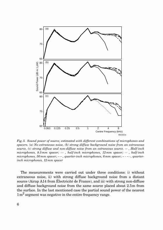
The measurements were carried out under three conditions: i) withoutextraneous noise, ii) with strong diffuse background noise from a distantsource (Airap A14 from Électricité de France), and iii) with strong non-diffuseand diffuse background noise from the same source placed about 2.5m fromthe surface. In the last mentioned case the partial sound power of the nearest1m2 segment was negative in the entire frequency range.

Fig. 5. Sound power of source, estimated with different combinations of microphones andspacers. (a) No extraneous noise, (b) strong diffuse background noise from an extraneoussource, (c) strong diffuse and non-diffuse noise from an extraneous source. –- , Half-inchmicrophones, 8.5 mm spacer; --- , half-inch microphones, 12 mm spacer; ··· , half-inchmicrophones, 50 mm spacer; – – , quarter-inch microphones, 6 mm spacer; – - – -, quarter-inch microphones, 12 mm spacer

960352e

Sou

nd P

ower

(dB

re

1 pW

)

60

70

80

60

70

80

60

70

80 (a)

(b)

(c)

0.250.1250.063 0.5 1 2 4 8Centre Frequency (kHz)


7

The measurements with quarter-inch microphones were carried out with a6mm spacer and with a 12mm spacer. The former measurement, which can beexpected to be reliable at high frequencies, served as the reference in the fre-quency range from 4 to 10kHz. The measurements with half-inch microphoneswere carried out with an 8.5mm spacer, a 12mm spacer and a 50mm spacer.In order to reduce the effect of transducer phase mismatch as far as possible,all measurements were repeated with the two microphones interchanged [4].

The results of the sound power measurements are presented in Fig.5; andFig.6, which shows the pressure-intensity index, gives an impression of theacoustic conditions. It can be seen from Fig.5 that practically all measure-ments are in agreement from 50Hz to 1.25kHz. An exception is the measure-ments with quarter-inch microphones at 50Hz under the most difficult soundfield condition. (This is probably the result of random errors due to electricalnoise [5]; however, without compensation for phase mismatch significanterrors occurred with the quarter-inch microphones in most of the frequencyrange.) From 1.6kHz and upwards the combination of half-inch microphonesand the 50mm spacer underestimates, but it is worth noting that the error isless than predicted by the idealised expression for an axial plane wave (Fig.1),and that the size of the error depends on the sound field conditions, whichleads to the conclusion that one cannot compensate for the finite differenceerror. The combination of quarter-inch microphones and a 12mm spacer leadsto underestimation from 5kHz and upwards, more or less as expected. The

Fig. 6. Pressure-intensity index. — , Quarter-inch microphones, 6 mm spacer, no extrane-ous noise; ---, half-inch microphones, 12 mm spacer, no extraneous noise‚ ···, quarter-inchmicrophones, 6 mm spacer, diffuse noise; – – , half-inch microphones, 12 spacer, diffusenoise; – · –. quarter-inch microphones 6 mm spacer, non-diffuse and diffuse noise: – - – -,half-inch microphones, 12 mm spacer, non diffuse and diffuse noise

960353e

10

∆pl (

dB)

00.250.1250.063 0.5 1 2 4

Centre Frequency (kHz)8


8

measurements with half-inch microphones and the 12mm spacer are in fairagreement with the reference measurements, confirming the predicted advan-tage of this combination. In fact, only the combination of half-inch micro-phones and the 8.5mm spacer behaves unexpectedly.

As can be seen, it overestimates slightly under mild measurement condi-tions, but underestimates under more difficult conditions. It seems as if theability of suppressing extraneous noise at high frequencies deteriorates if thespacer is significantly shorter than the diameter of the microphones. A possibleexplanation is that the error depends more on the angle of incidence for thisconfiguration, cf. Fig.3.

ConclusionsOne cannot compensate for the finite difference error of p-p intensity probesby using the theoretical plane wave expression, and one cannot extend the fre-quency range by using a spacer appreciately shorter than the diameter of themicrophones. Moreover, existing quarter-inch microphones are not suitablefor measurement of sound intensity at low frequencies. However, a numericaland experimental study of diffraction effects has demonstrated that the opera-tional frequency range can be extended to an octave above the limit deter-mined by the finite difference error if the length of the spacer between themicrophones equals the diameter. This means that a probe with half-inchmicrophones can cover the frequency range from 50Hz to 10kHz.

References[1] FAHY, F.J.: “Sound Intensity” (E & FN Spon (second ed.), London 1995)

[2] WATKINSON, P.S.: and FAHY, F.J.:J. Sound Vib. 94, 299-306 (1984)

[3] CUTANDA, V.: JUHL P.M. and JACOBSEN, F. : “A numerical investi-gation of the performance of sound intensity probes at high frequencies”Proc. Fourth Int. Congress on Sound and Vib., 1996, pp. 1897 – 1904

[4] REN, M.: and JACOBSEN, F.: Noise Control Eng. J. 38, 17-25 (1992)

[5] JACOBSEN, F.: J. Sound Vib. 166, 195-207 (1993)

bv004811.book : MicFree-field Black 9

9

Measurement of Microphone Free-fieldCorrections and Determination of theirUncertainties

by Erling Frederiksen and Johan Gramtorp

AbstractModern measurement techniques and international cooperation on calibra-tion research have made it possible to obtain more accurate free-field and dif-fuse-field corrections. In this article the methods and measurements aredescribed and calculations of the uncertainties for the free-field corrections formicrophone Type 4191 (12.5mV/Pa) are shown.

RésuméLes techniques de mesure modernes et la coopération internationale dans larecherche sur le calibrage ont contribué à améliorer la précision des correctionsde champ libre et de champ diffus. Cet article décrit les différentes méthodes demesure utilisées et présente un calcul d’incertitude pour les corrections champlibre du Microphone Type 4191 (12.5mV/Pa).

ZusammenfassungModerne Meßtechnik und internationale Zusammenarbeit auf dem Gebietder Kalibrierung ermöglichen eine höhere Präzision bei Freifeld- und Diffus-feldkorrekturen. Dieser Artikel beschreibt die verschiedenen Meßmethodensowie die Berechnung der Unsicherheit der Freifeldkorrektur für das Mikro-fon Typ 4191 (12,5mV/Pa).

IntroductionThe most commonly used method for frequency response calibration of measure-ment microphones is still to measure the individual electrostatic actuatorresponse and to add corrections to this. The corrections are the same for allmicrophones of the same type. For well-documented microphone types, free-field


10

and diffuse-field corrections are available from the microphone manufacturers.Brüel&Kjær has recently developed a new line of 1/2″ microphone types (FalconRange) and has determined their corrections which are to be used for calibrationat the factory and at calibration service laboratories abroad.

The principles applied for the determination of these free-field and diffuse-field corrections are the same as those used in the past but modern measure-ment techniques and international co-operation on calibration research havesignificantly improved the possibilities for obtaining more accurate correc-tions. Today, many countries and companies are improving their calibrationsystems. Therefore, there is an increasing demand for accurate correctionswith documented uncertainty. The methods, the measurements and the uncer-tainties related to the resulting corrections for Type 4191 (12.5 mV/Pa) are dis-cussed in this article.

Description of Free-field and Diffuse-fieldCorrectionsThe free-field correction is the ratio between the free-field response and theresponse of the microphone diaphragm system, Fig.1. The correction is domi-nantly determined by sound reflection and refraction caused by the micro-phone body. There are two different types of free-field corrections. They refer

Fig. 1. Free-field Frequency Response of a Type 4191 microphone obtained by adding theFree-field Correction to an individually measured Actuator Response

960368e

– 12

– 10

– 8

– 6

– 4

– 2

0

2dB

100 1000 10000 100000Frequency (kHz)

Free-field Response

Free-field Correction

Actuator Response


11

to the slightly different pressure and actuator responses. Both responsesaccount for the individual properties of the microphone diaphragm systems.They are relatively easy to measure in comparison with the free-fieldresponse. Actuator response calibrations are especially simple and require nospecial acoustic facilities. The Diffuse-field Response can be determined in thesame way by applying other corrections to the actuator response.

Free-field Response MeasurementThree microphones were calibrated together. Pair-wise they were mounted inan anechoic room where one was transmitting sound to another. Microphone(a) transmitted to receiver (b), (b) to (c) and (c) to (a).

In order to minimise the influence of room reflections a rather large room ofapprox. 4m × 4.5m × 5m open space and a relatively short measurement dis-tance (0.23m) were chosen.

The international standard IEC1094-3 defines the free-field sensitivityproduct, Mf,a. Mf,b by the formula (A). A modification of this eliminates thetransmitter current and leads to the applied formula (B).

(A)

(B)

UR,b : Receiver output voltageUT,a : Transmitter driving voltagedab: Distance between acoustic centres of the microphonesρ: Air densityf : FrequencyCa : Transmitter Capacitance∝ : Sound attenuation of air

For all three pairs of microphones the output voltage of the receiver micro-phone, the voltage driving the transmitter and the transmitter capacitance

Mf a, Mf b,⋅ jUR b,

IT a,

2dab

ρ f⋅e

αdab⋅ ⋅ ⋅−=

Mf a, Mf b,⋅UR b,

UT a,−

dab

ρ π f 2 Ca⋅ ⋅ ⋅e

αdab⋅ ⋅=


12

were measured. During the measurement of the receiver voltage, the voltageacross the transmitter was kept constant as a function of frequency. For flatmicrophone frequency responses this leads to a sound pressure and a receiveroutput which increase by 40 dB/decade and are very low at 1000Hz where themeasurements should preferably start; see Fig.2.

Fig. 2. Receiver Microphone Output Voltage as a function of frequency

Fig. 3. Free-field Calibration System operating to 200 kHz. The possible accuracy is betterthan 0.025 dB at 0 dB SPL

960369e

80

70

60

50

40

30

20

10

01 10

dB re. 1 µV

Frequency (kHz) 100

960370e

MeasurementMonitor

ReceiverMicrophones

Transmitter

MeasurementAmplifier

Type 2636

IEC-bus

DigitalInterface

for Type 2010

Controller

A/DConverter

Free-fieldMeasurement System

Terminal

VAXComputer

ModifiedNarrowBand

AnalyzerType 2010

Amplifier20 dB


13

To overcome problems with the signal to noise ratio Brüel&Kjær built adedicated free-field calibration system some years ago. The system can workup to 200kHz and thus cover the frequency range of most types of measure-ment microphones (sizes from 1″ to 1/8″). A block diagram of this system isshown in Fig.3. The measurements were performed with this system at fre-quency steps of 100Hz with a spread and a resolution better than 0.025dB.Synchronous sampling and measurement times of up to half an hour at each ofthe lowest frequencies were used for improving the S/N-ratio.

After determination of the above parameters for the three pairs of micro-phones, the sensitivity products and the individual free-field sensitivity mod-ule were calculated using the formula below.

Electrostatic Actuator Response CalibrationThe actuator responses were measured with 0.01dB resolution and with thesame measurement system as that used for the free-field measurements. Thistype of measurement is relatively easy to perform. The uncertainty of actuatorcalibration is high with respect to the absolute sensitivity. This is typically ofthe order 1dB while it is very low for the frequency response calibration.

The response measured with an electrostatic actuator is generally influ-enced by the radiation impedance which loads the microphone diaphragm. ForType 4191, which has a relatively high diaphragm impedance, the influenceranges from essentially zero at low frequencies to about 0.3dB at the highestfrequencies (40 kHz). As the influence may be modified by the mechanical con-figuration of the actuator, the actuator type used for calibration service shouldbe equal to that used for determination of the corrections.

Mf a,

UR a, UR c,⋅UR b,

UT b,

UT a, UT c,⋅dab dca⋅

dbc⋅ ⋅

=

Cb

Ca Cc⋅1

ρ π f 2⋅ ⋅e

α dab dbc d+ca

−( )⋅ ⋅ ⋅

1

2


14

Measured and Calculated Free-field CorrectionsAs mentioned above, the absolute sensitivity cannot be measured accuratelywith an electrostatic actuator. Therefore, there is no reason for also spendinggreat efforts on obtaining an absolute measurement of the free-field response.The division of the free-field response by the actuator response will, anyway,give a result which contains a significant error. However, as this error makesa constant factor over the entire frequency range, some methods are availablefor its elimination.

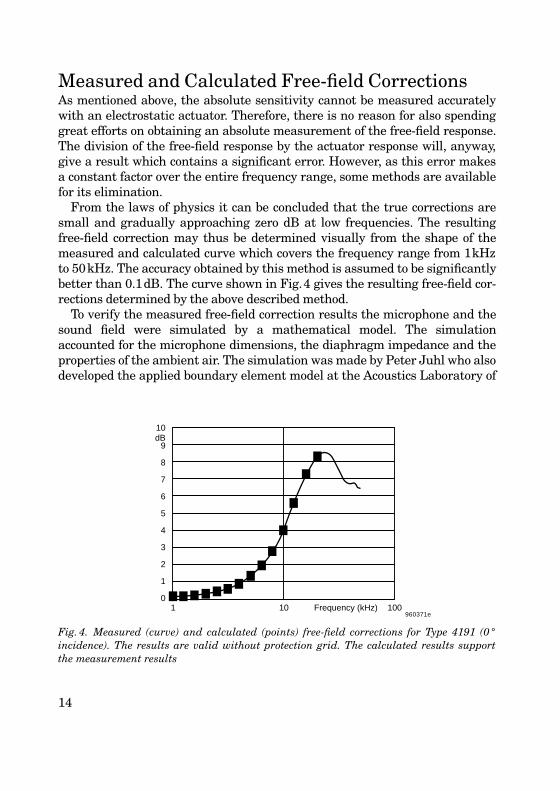
From the laws of physics it can be concluded that the true corrections aresmall and gradually approaching zero dB at low frequencies. The resultingfree-field correction may thus be determined visually from the shape of themeasured and calculated curve which covers the frequency range from 1kHzto 50kHz. The accuracy obtained by this method is assumed to be significantlybetter than 0.1dB. The curve shown in Fig.4 gives the resulting free-field cor-rections determined by the above described method.

To verify the measured free-field correction results the microphone and thesound field were simulated by a mathematical model. The simulationaccounted for the microphone dimensions, the diaphragm impedance and theproperties of the ambient air. The simulation was made by Peter Juhl who alsodeveloped the applied boundary element model at the Acoustics Laboratory of

Fig. 4. Measured (curve) and calculated (points) free-field corrections for Type 4191 (0 °incidence). The results are valid without protection grid. The calculated results supportthe measurement results

960371e

8

9

10

7

6

5

4

3

2

1

01 10

dB

Frequency (kHz) 100


15

the Technical University in Lyngby, Denmark. The 1/3 octave calculationresults are shown by the points in Fig.4.

These results support the measurement results, especially at low frequen-cies while they are probably less reliable at the high frequencies due to lack ofsufficient spatial resolution of the model.

Measurement of Directional Responses

The free-field correction discussed above is valid for 0° incidence (referencedirection). The sensitivities and corrections for other angles of incidence weredetermined relative to 0° for angle steps of 5° by the set-up shown in Fig.5. Thesound source was mounted in a fixed position while the receiving microphonewas rotated to its different angles by an automatic turntable. The necessary,rather long, measurement distance and the turntable arrangement will gener-ally lead to disturbing reflections. Therefore, a TDS measurement systembased on the Brüel&Kjær Type 2012 was applied. This system makes timeselective measurements and can eliminate reflections. The directional charac-teristics obtained are shown in Fig.6.

Fig. 5. The time selective measurement system for directional responses eliminatesreflections

960372e

TurntableControllerType 5949

TurntableType 5960

TDS Measurement System

AudioAnalyzer

Type 2012

Microphone

PowerAmplifier

Type 2706


16

Random Incidence CorrectionsThe random incidence correction is calculated in accordance with the Interna-tional Standard IEC1183 (1994/95) which specifies how the calculation shouldbe made. The free-field corrections shown in Fig.6 were applied with weight-ing factors which account for that fraction of total power coming to the micro-phone from the specific directions. The resulting random incidence correctionis also shown in Fig.6.

Estimated Uncertainty of Free-field CorrectionsThe resulting uncertainties of the 0° free-field correction were estimated fromthe uncertainties of the parameters applied for its calculation. Their uncer-tainties were separated into groups of random and systematic errors as theirweight in the reciprocity calculations are different. The systematic errors dopartly eliminate each other while the non correlated or random errors add upstatistically. The relative uncertainty of Free-field Response was determinedby using the formula below:

Fig. 6. Free-field corrections for Type 4191 without protection grid. The angles are steppedby 5 degrees


17

where the weighting factor ‘A’ equals 1/2 for the systematic and for therandom uncertainties respectively. After determination of other uncertaintiesrelated to the actuator response, the low frequency normalisation of the free-field corrections to 0dB and to the influences of ambient pressure and temper-ature, the resulting uncertainty was calculated.

The uncertainty (tentative) of the free-field corrections for Type 4191 with-out grid was estimated to:

Notes:The uncertainty (95% confidence level) is valid for the 0°-correction at101.3kPa, 23°C and 50% RH.

To calculate the uncertainty of a calibration for which the correction isapplied, the uncertainty of the electrostatic actuator calibration must be takeninto account. It should also be noted that the uncertainty of calibrations validfor microphones with protection grid are generally higher.

ConclusionFree-field corrections were worked out for a new line of 1/2″ measurementmicrophones. The uncertainty of the Type 4191 free-field correction (0°-inci-dence) was analysed and calculated. The result agrees well with the uncer-tainty estimated from practical experience. The new corrections representimprovements in comparison with the corrections and the uncertainty esti-mated for earlier microphone types. The analysis revealed possibilities for fur-ther improvements in the future.

Frequency 1kHz 2kHz 4kHz 8kHz 16kHz 32kHz 40kHz

Uncertainty (2×σ) 0.03dB 0.06dB 0.08dB 0.10dB 0.12dB 0.15dB 0.20dB

∆Mf

MfA

∆UR

UR

2

⋅∆UT

UT

2 ∆C

C

2 ∆f 2

f 2

2 ∆d

d

2 ∆ρρ

2

+ + + + +=

αd∆αα

2

αd∆d

d

2

+ +

1

2

3 2⁄


18

References[1] IEC486, “Precision method for free-field calibration of one-inch stand-

ard condenser microphones by the reciprocity technique and the draft forthe succeeding IEC document which includes 1/2″ microphones

[2] RASMUSSEN,K.: and SANDEMANN OLSEN, E.: “Intercomparisonon free-field calibration of microphones”, Final report (PL-07), theAcoustics Laboratory, Technical University of Denmark

[3] JUHL, P.: “Numerical Investigation of Standard Condenser Micro-phones” Journal of Sound and Vibration 1994 Vol. 177 (4) p. 433-446

bv004811.book : Non-linear Black 19

19

Reduction of Non-linear Distortion inCondenser Microphones by UsingNegative Load Capacitance

by Erling Frederiksen

AbstractAn analysis was made of the distortion produced by condenser measure-ment microphones which operate with stiffness controlled diaphragms. Acalculation formula which was theoretically derived was verified by exper-iments. Analysis of this formula indicated that the distortion can bereduced by loading the microphone with a proper capacitance which has tobe negative and is a function of the ratio between the backplate and dia-phragm diameters. Experimental results confirmed this.

RésuméNous avons analys la distorsion produite par les microphones de mesure con-densateur quips de diaphragmes dont la tension tait contrle. Une formule,rsultat dune approche thorique, indiquait que lon peut rduire le phnomne dedistorsion en chargeant le microphone avec une capacit approprie, qui doit trengative et tenir compte du rapport entre les diamtres du diaphragme et de laplaque arrire. Cest ce quont confirm les expriences ralises.

ZusammenfassungEs wurde die Verzerrung analysiert, die Kondensatormeßmikrofone auf-weisen, wenn die Auslenkung der Membran durch ihre Steifigkeitbestimmt wird. Eine theoretisch abgeleitete Berechnungsformel wurdeexperimentell bestätigt. Die Analyse der Formeln wies darauf hin, daß sichdie Verzerrung reduzieren läßt, wenn das Mikrofon mit einer geeignetenKapazität belastet wird. Diese Kapazität ist negativ und eine Funktion desQuotienten aus den Durchmessern von Gegenelektrode und Membran. Daswurde durch Versuchsergebnisse bestätigt.


20

IntroductionCondenser measurement microphones have very wide dynamic ranges, typi-cally 140dB. At low sound levels the range is limited by inherent noise of themicrophone and/or preamplifier. At high levels it is generally limited by non-linear distortion which is proportional to the sound pressure and is producedby the microphone itself. This distortion has been analysed in theory and inpractice for some frequently used types of microphones. The good agreementwhich was found between measured and calculated results verifies thederived distortion formulae and points clearly at the load capacitance andmode of diaphragm displacement as being the dominating reasons. The for-mulae were used for calculation of the capacitive loading which would lead tothe lowest possible distortion. This appeared to be negative and to be a func-tion of the ratio between the backplate and diaphragm diameters. Tests madewith an experimental preamplifier with negative input capacitance gavepromising results.

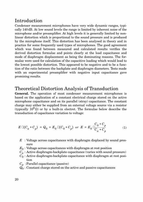
Theoretical Distortion Analysis of TransductionGeneral. The operation of most condenser measurement microphones isbased on the application of a constant electrical charge stored on the activemicrophone capacitance and on its parallel (stray) capacitance. The constantcharge may either be supplied from an external voltage source via a resistor(typically 109Ω) or by a built-in electret. The formulae below describe thetransduction of capacitance variation to voltage:

(1)

E : Voltage across capacitances with diaphragm displaced by sound pres-sure

E0 : Voltage across capacitances with diaphragm at rest positionCa : Active diaphragm-backplate capacitance (varies with sound pressure)C0 : Active diaphragm-backplate capacitance with diaphragm at rest posi-

tionCp :Parallel capacitance (passive)Q0 : Constant charge stored on the active and passive capacitances

E Ca Cp+( )⋅ Q0 E0 C0 Cp+( ) or E⋅ E0

C0 Cp+

Ca Cp+⋅= = =


21

As the charge (Q0) is kept constant the voltage (E) will vary with the varia-tion of the active capacitance (Ca) which is caused by the sound pressure. Thevoltage produced depends on the microphone configuration and on the dia-phragm deflection mode.

Flat Diaphragm Displacement ModeIf the microphone diaphragm is considered to be parallel to a circular back-plate and displaced like a flat piston, then the active capacitance (Ca) and itsrest capacitance (C0) can be expressed by the equations:

where and

ε : Dielectric constant of airRb : Radius of backplateD : Rest distance, backplate to diaphragmd : Displacement of diaphragmRs : Ratio of effective and total backplate areaAb : Total backplate area (includes area of holes)Ah : Area of holes in backplate (a uniform hole distribution is considered)y : Relative diaphragm displacement

Fig. 1. Microphone with flat diaphragm displacement mode and parallel capacitance

Ca Rs

ε π Rb2⋅ ⋅

D d+⋅ C0 1 y+( ) 1−⋅= =

C0 Rs

ε π Rb2⋅ ⋅

D⋅= Rs

Ab Ah−

Ab= y

dD

=

960363e

D dCa

Cp


22

Insertion of the above expressions into Equation (1) leads to Equation (2)which defines the output voltage of a microphone with a flat diaphragm dis-placement mode:

(2)

Series expansion of equation (2) leads to:

(2a)

For a sinusoidally varying diaphragm displacement with time y, y2 and y3

become:

where ym : Maximum value of relative diaphragm displacement.

This leads to the following second (D2) and third (D3) harmonic distortioncomponents of the output voltage (relative to the fundamental frequency com-ponent):

The dominating second harmonic component (D2) is proportional to the dia-phragm displacement and thus to the sound pressure while the third harmonic(D3) is proportional to the square of the pressure. Notice, that the distortiondecreases with the parallel capacitance and that it becomes zero if this capaci-tance becomes zero (Cp = 0).

Efm E0

C0 Cp+

C0 1 y+( ) 1− Cp+⋅⋅=

Efm E0 E0+C0

C0 Cp+y

Cp

C0 Cp+

1

y2Cp

C0 Cp+

2

y3 .....−⋅+⋅− ⋅ ⋅=

y ym ωt; y2sin⋅ 12

ym2 1 2ωtcos−( ) ; y3⋅ ⋅ 1

4ym3 3 ωt 3ωtsin−sin( )⋅ ⋅= = =

D212

ym

Cp

C0 Cp+⋅ ⋅

1

100% and D3⋅ 12

ym

Cp

C0 Cp+⋅ ⋅

2

100%⋅= =


23

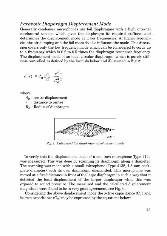
Parabolic Diaphragm Displacement ModeGenerally condenser microphones use foil diaphragms with a high internalmechanical tension which gives the diaphragm its required stiffness anddetermines the displacement mode at lower frequencies. At higher frequen-cies the air damping and the foil mass do also influence the mode. This discus-sion covers only the low frequency mode which can be considered to occur upto a frequency which is 0.2 to 0.5 times the diaphragm resonance frequency.The displacement mode of an ideal circular diaphragm, which is purely stiff-ness controlled, is defined by the formula below and illustrated in Fig.2:

whered0 : centre displacementr : distance to centreRd : Radius of diaphragm

To verify this the displacement mode of a one inch microphone Type 4144was measured. This was done by scanning its diaphragm along a diameter.The scanning was made with a small microphone (Type 4138, 1.8 mm back-plate diameter) with its own diaphragm dismantled. This microphone wasmoved at a fixed distance in front of the large diaphragm in such a way that itdetected the local displacement of the larger diaphragm while this wasexposed to sound pressure. The measured and the calculated displacementmagnitude were found to be in very good agreement; see Fig.3.

Considering the above displacement mode the active capacitance (Ca ) andits rest capacitance (C0 ) may be expressed by the equations below:

Fig. 2. Calculated foil diaphragm displacement mode

d r( ) d0 1r2

Rd2

− ⋅=


24

where

Simplification and integration of the above equation leads to:

Fig. 3. Diaphragm displacement as a function of distance to centre for a one inch micro-phone with a diaphragm of 18 mm diameter. The points are measured at 40 Hz and at130 dB and 150 dB SPL. The curve is calculated

960365e

Dis

plac

emen

t re.

Cen

tre

– 10

100

80%

60

40

20

0– 8 – 6 – 4 – 2 0 2 4 6 8

Distance from Centre (mm)10

Ca Rsε 2 π r⋅ ⋅ ⋅

D d0 1r2

Rd2

− ⋅+

dr C0

0

Rb

∫⋅ Rs

ε π Rb2⋅ ⋅

D⋅= =

Rs

Ab Ah−

Ab=

Ca Rs

ε π Rb2⋅ ⋅

DRb

2−

0

Rb

∫ 2 r⋅

1 y0 1r2

Rd2

− ⋅+

dr⋅ ⋅ ⋅=


25

where and

Insertion of Ca and C0 in Equation (1) gives the equation valid for parabolicmode:

(3)

Series expansion of Equation (3) leads to:

(3a)

where

Ca C0 Rb2− 2 r⋅

1 y0+ 1r2

Rd2

− ⋅

dr

0

Rb

∫⋅ ⋅=

Ca Co

Rb2

Rd2

1−

y01− ln

1 y0+

1 1Rb

2

Rd2

−

y0⋅+

⋅ ⋅ ⋅=

Ca C0 1 k−( ) 1− y01− ln

1 y0+

1 k y0⋅+⋅ ⋅ ⋅=

k 1Rb

2

Rd2

−= y0

d0

D=

Epm E0

C0 Cp+

C0 1 k−( ) 1− y01− ln

1 y0+

1 k y0⋅+Cp+⋅ ⋅ ⋅

⋅=

Epm E0 E0k 1+

2

C0

C0 Cp+y0 F2 y0

2 F3 y03 ....+⋅+⋅+( )⋅ ⋅ ⋅+=


26

and

The factors F2 and F3 are functions of the parameter k and thus of the ratiobetween the backplate and diaphragm radii. The larger the backplatebecomes, the higher becomes the distortion. Equation (2a) indicates that thiseffect was to be expected as area added along the outer circumference repre-sents a less active capacitance which loads the more active capacitance locatedat the diaphragm and backplate centres.

Notice, that the smaller the backplate becomes in comparison with the dia-phragm, the more flat does the active part of the diaphragm becomes. There-fore, for k equal to ‘1’, Equation (3a) becomes equal to Equation (2a) which isvalid for flat diaphragm mode. In practice, distortion should be defined as afunction of Sound Pressure (p) rather than relative diaphragm displacementat the centre (y0). The relation between displacement and sound pressure canbe obtained from the following equations:

e1 : Microphone output voltage according to Equation (3a)(1st term with y0)

p : Sound pressureS0 : Measured open circuit sensitivity

For a sinusoidal diaphragm displacement with time, the ratios (D2 and D3)between the second and third harmonic components and the fundamentalcomponent become:

F2

C0 k2 2 k 1+⋅−( ) 4 Cp k2 k 1+ +( )⋅ ⋅+⋅

6 C0 Cp+( ) k 1+( )⋅ ⋅−=

F3

C02 4 C0 Cp⋅ ⋅+( ) k2 2 k 1+⋅−( ) 6 Cp

2 k2 1+( )⋅ ⋅+⋅

12 C0 Cp+( ) 2⋅=

e1 E0k 1+

2

C0

C0 Cp+y0 and p⋅ ⋅ ⋅ e1 S0

C0 Cp Ci−+

C0 Cp+⋅

1−⋅= =


27

(4)

and

(5)

where

Comparison of Calculated and Measured DistortionCalculated and measured distortion data were evaluated by comparison. Seeinput data and distortion results for some commonly used microphones in thetables below.

B&K Type No. 4144 4133 4165 4135 4190 4192/93

Dimension 1/1″ 1/2″ 1/2″ 1/4″ 1/2″ 1/2″

S0 mV/Pa 50 12 50 4.0 50 12.5

E0 V 200 200 200 200 200 200

Rd mm 9.1 4.6 4.6 2.1 4.6 4.6

Rb mm 6.65 3.60 3.65 1.75 3.45 3.45

D0 µm 23.5 21.0 22.2 18.0 24.5 19.0

Ah mm2 20.3 1.70 4.24 0 3.96 5.50

Ce pF 2.1 0.5 0.9 0.2 0.8 0.8

Ch pF 2.1 1.1 1.8 1.6 1.6 1.5

D2

ym

2 1

F2 100%⋅ ⋅=

D3

ym

2 2

F3 100%⋅ ⋅=

ym 2 pRMS

S0

E0

C0 Cp C i−+

C0

2k 1+

⋅ ⋅ ⋅ ⋅=


28

There is very good agreement between the calculated and the measured dis-tortion data. The calculated ratio (see lower table) is very close to one. As thecalculations only account for the transduction itself this seems to be the onlysource of low frequency distortion which is of importance for the analysedtypes of microphones.

Distortion Reduction By Negative CapacitanceLoadingTheoryEquation (4) shows that the 2nd harmonic component is proportional to thefactor F2. It is a function of the ratio between the active and the passive paral-lel capacitances as well as of the ratio between the backplate and diaphragmradii. For a certain radii ratio (i.e. a certain value of ‘k’) F2 and the second har-monic distortion become zero if the microphone is loaded with a proper nega-tive capacitance. Calculated distortion is shown for two extreme microphoneconfigurations in Fig.4.

B&K Type No. 4144 4133 4165 4135 4190 4192 4193

LoadCapacitance pF 0.2 0.2 0.2 0.2 0.2 0.2 100

Sound PressureLevel

dB 140 150 140 160 140 150 150

2. harm.calculated % 0.51 0.49 0.97 1.52 0.97 0.63 3.0

2. harm.measured * % 0.56 0.50 1.08 1.55 0.90 0.54 3.4

Ratio - Calc.re. HB-data

0.91 0.97 0.98 0.98 1.08 1.17 0.88

3. harm.calculated % 0.01 0.01 0.02 0.04 0.02 0.01 0.09

* Sources: Brüel & Kjær’s blue Microphone Handbook and the Falcon Handbook. The data appliedfor Types 4133 and 4165 originates from measurements performed in January 1994


29

Typical microphone/preamplifier combinations have a Cp /C0-ratio of +0.1to +0.4. Fig. 4 shows that the optimum with respect to distortion is between‘−0.25’ and ‘0’. The ideal Cp /C0-ratio is defined by the following equation:

Negative CapacitanceIn principle, negative load capacitance may be created by a circuit like thatshown in Fig. 5. A capacitor (C) is connected between the input and output ofthe microphone preamplifier whose gain (>+1) can be adjusted to give theproper input capacitance (Ci); see the formula:

where e1: input voltage, e2: output voltage

Fig. 4. Harmonic distortion calculated as a function of the ratio between the passive andactive capacitances

960366e

Dis

tort

ion

– 0.5 – 0.4 – 0.3 – 0.2 – 0.1 0 0.1 0.2 0.3 0.4 0.5 0.6 0.7 0.8 0.9 10.001

0.01

0.1

1

10

%

Ratio between Cp and Co

2. Harmonic

Large Backplate (k = 0)

Small Backplate (k = 1)

3. Harmonic

Cp

C0

ideal

14

− k2 2 k 1+⋅−

k2 k 1+ +⋅=

Ci

e1 e2−

e1C⋅ 1 A−( ) C⋅= =


30

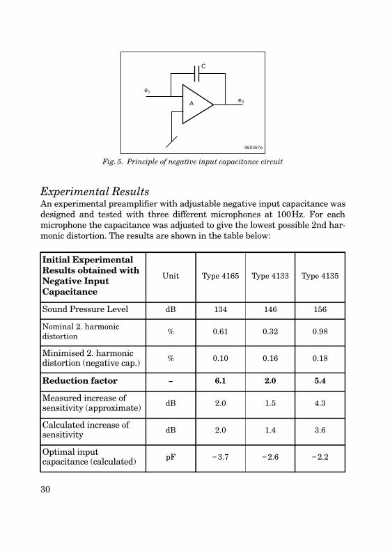
Experimental ResultsAn experimental preamplifier with adjustable negative input capacitance wasdesigned and tested with three different microphones at 100Hz. For eachmicrophone the capacitance was adjusted to give the lowest possible 2nd har-monic distortion. The results are shown in the table below:

Fig. 5. Principle of negative input capacitance circuit

Initial ExperimentalResults obtained withNegative InputCapacitance

Unit Type 4165 Type 4133 Type 4135

Sound Pressure Level dB 134 146 156

Nominal 2. harmonicdistortion

% 0.61 0.32 0.98

Minimised 2. harmonicdistortion (negative cap.) % 0.10 0.16 0.18

Reduction factor – 6.1 2.0 5.4

Measured increase ofsensitivity (approximate) dB 2.0 1.5 4.3

Calculated increase ofsensitivity dB 2.0 1.4 3.6

Optimal inputcapacitance (calculated) pF −3.7 −2.6 −2.2

960367e

A

C

e1

e2


31

The idea (patented) of using negative input capacitance for distortion reduc-tion seems to work well in practice but further experiments have to be made toclarify all aspects of its use. The Brüel&Kjær High Pressure Calibrator Type4221 was used for the distortion measurements.

ConclusionHarmonic distortion of condenser microphones using constant electricalcharge has been analysed for the frequency range where the diaphragm dis-placement is stiffness controlled. Distortion formulae have been derived forthe transduction from diaphragm displacement to output voltage. The formu-lae were applied for calculating distortion of some commonly applied types ofmeasurement microphones. The results were compared with data supplied bythe manufacturer and very good agreement was found. This verified the for-mulae and pointed at parallel capacitance and displacement mode as beingthe dominating reason for the distortion. The distortion analysis indicated thepossibility of reducing harmonic distortion by loading the microphone withnegative capacitance. This was confirmed by experiments.

Further work has to be done to analyse the practical possibilities which inaddition to distortion reduction might be improvement of high level peakmeasurements and extension of the applicable dynamic range of condensermicrophones.

bv004811.book : In-situ Black 32

32

In Situ Verification of AccelerometerFunction And Mounting

by Torben R. Licht

AbstractPiezoelectric accelerometers are used for vibration measurements in a hugevariety of measurement situations. Many different ways of checking theintegrity of a measurement channel have been devised, from tapping on thestructure to very sophisticated measurement schemes such as compleximpedance measurements. A new practical charge amplifier input systemwhich permits in situ check of accelerometer functionality and mounting per-formance has been developed. (Patent pending). A description of the systemand performance examples will be given.

RésuméLes accéléromètres piézoélectriques interviennent dans de nombreux types demesures vibratoires. De nombreuses méthodes de vérification de l’intégrité dela chaîne de mesure ont été mises en œuvre, des simples impacts sur la struc-ture jusqu’à des dispositifs de mesure d’impédance complexe. Un nouveau sys-tème d’entrée d’amplification de charge très pratique vient d’être mis au pointpour permettre la vérification in situ des fonctionnalités de l’accéléromètre etdes performances de l’installation (en instance de brevet). Il est décrit dansces pages et ses performances sont illustrées par des exemples.

ZusammenfassungPiezoelektrische Beschleunigungsmesser werden für eine Vielzahl vonSchwingungsmessungen verwendet. Um die Integrität des Meßkanals zuprüfen, wurden zahlreiche Methoden entwickelt, vom Beklopfen der Strukturbis zu hochkomplizierten Meßverfahren wie die Messung der komplexenImpedanz. Es wurde ein neues praktisches Ladungsverstärker-Eingangssy-stem entwickelt, mit dem sich Funktionstüchtigkeit und Befestigung vonBeschleunigungsaufnehmern in situ prüfen lassen. (Patent angemeldet). Esfolgen eine Beschreibung des Systems und Beispiele für seine Leistungsfähig-keit.


33

IntroductionPiezoelectric accelerometers are used extensively to measure vibration onmany different structures and with many different vibration sources.

A number of different techniques are used to ensure the proper functioningof each measurement channel, but only a few very complicated methods havebeen used to verify the mechanical integrity of the transducer and its mount-ing.

This is even more serious because the handling and mounting are often car-ried out by people without knowledge of vibration measurement techniques.

Both statistics and an educated guess indicate that, on a list of commonproblems with piezoelectric accelerometers, the first is cabling and the secondis mounting.

Therefore it is believed that the simple method for testing mounted trans-ducers, described in the following, can make a significant contribution to thequality of future vibration measurements.

Accelerometer TheoryNormally an accelerometer is described as a seismic transducer with the sim-ple model shown below. k is the stiffness of the spring, c the damping and mthe seismic mass.

The ratio between the motion amplitude of the moving part and the relativemotion of the mass with respect to the housing can be described in magnitudeand phase by the formulae

Fig. 1

960354e

k

c

m

Moving Part


34

where d=c/cc is the fraction of critical damping and

is the resonant angular frequency.

For accelerometers the input is taken as acceleration of the moving part yield-ing Ra=−Rd/ω2. The resulting general curves are shown here.

Fig. 2 Fig. 3

Rd

ωωr

2

1ω

ωr

2−

2

2dωωr

2

+

and θ tan 1−2d

ωωr

1ω

ωr

2−

= =

cc 2 km 2mωr= =( )

ωrkm

=

960355e

Frequency/Resonant Frequency

Seismic Transducer Phase Response

d = 0.01d = 0.1

Rel

. Dis

plac

emen

t/Inp

ut A

ccer

atio

n (d

egre

es) 180

150

120

90

60

30

00.1 1 10

d = 0.2d = 0.707

960356e

Frequency/Resonant Frequency

Seismic Transducer Response

Rel

. Dis

plac

emen

t/Inp

ut A

ccer

atio

n

100

10d = 0.01

d = 0.1

d = 0.2

d = 0.7071

0.1

0.010.1 1 10


35

Practically all piezoelectric accelerometers have a negligible damping in theorder of 0.01, which means that the resonance peak has a high Quality FactorQ, making it possible to excite the resonance and observe the decaying signal.To include the mounting, the model has to be extended to the following wherethe base and mounting stiffness is included as separate items and the dampinghas been omitted.

The normal modes of such a system is described by the roots of the equation

or

giving the roots

where R = K/k is the ratio between the two spring constants andis the mounted resonance frequency.

Fig. 4960357e

k

K

m

Base M

Structure

Mω2 k K+( )−k

k

mω2 k−0=

Mmω4 m( k K+( )− Mk ) ω2 kK+ + 0=

ω2 ωm2

1R2

1R2

2

+±+=

ωmkm

=


36

The two modes described by the formula are shown in the graph below.

Test MethodThe basic idea of the test method is based on the reciprocal nature of the pie-zoelectric material, i.e. if a voltage is applied to the piezoelectric discs they willchange shape, following the general equation

where dxy is the appropriate piezoelectric constant, mostly d33 (compressionconstructions) or d15 (shear constructions).

This implies that on transducer designs with low damping and relativelyhigh coupling (high d) an electrical pulse can be used to excite the structureand make it “ring” or vibrate at its resonance frequency for an extended periodof time.

The decrease in amplitude is given by the logarithmic decrement

Fig. 5

960358eSpring Constant Ratio

System Modes

Mode 2

Mode 1

Mod

e F

requ

ency

/Mou

nted

Res

onan

ce F

requ

ency 10

1

0.010.1 1 10

∆x dxy V⋅=

∆ 2πd≈


37

which for a damping d = 0.01 gives ∆=0.06 i.e. the amplitude decreases 6% peroscillation, leaving a number of oscillations in the order of 50 to be observed.

The frequency observed will be the dominant mode of the two shown above.A well mounted accelerometer, i.e. where a high spring constant ratio isobtained, will then resonate at the mounted resonance frequency. However,the more loose the mounting becomes, the lower will that mode frequency beand the more the free hanging resonance will become dominant. This gives 1.4times the mounted resonance in the typical case shown in the figure.

The amplitude of the signal can be used as a check on the accelerometer sen-sitivity squared.

ImplementationIn the Brüel&Kjær Measuring Amplifier Type 2525 a function has beenimplemented to exploit the idea described previously.

The instrument contains a generator which can generate a single squarepulse, as well as the logical circuitry to switch the generator in and out in frontof the charge amplifier. The time signal is shown schematically below.

A counter with gating is also included in the amplifier. This permits thedirect display of the measured resonance frequency of the system tested.

Fig. 6

960359e

Time, typically microseconds

Inpu

t and

Out

put S

igna

l Am

plitu

des

20

15

10

5

0

– 5

– 10

– 15

– 20200 400

Input and Output time records

600 800 10000


38

Examples of ApplicationAn accelerometer Type 4382 with a specified mounted resonance frequency of28 kHz ±10% and a mass of 17 grams was mounted on a large steel block. Agood, smooth surface was present at the mounting position.

The measured resonance frequency as a function of the mounting torquewas measured. The results are shown in Table 1.

The results show that when a good mounting surface is made the torque isnot critical for low level measurements (at higher vibration levels the trans-ducer might lose contact to the surface with dramatic errors as a result).

To simulate a bad surface a single 0.18mm (0.007″) strand of copper wirewas introduced between the accelerometer and the mounting surface. A fre-quency of 21.28kHz was measured, which shows the dramatic change from26,87 to 21.28kHz on the resonance.

Another experiment was made to show the kind of information which can beobtained.

A plate has a certain local stiffness, i.e. in principle, a certain mechanicalimpedance. When we mount an accelerometer of a certain mass M, i.e. a cer-tain mechanical impedance equal to jωM, we load the plate and change itsparameters, e.g. the resonance frequencies according to the ratio between thetwo impedances.

If the plate impedance is large compared to the accelerometer impedancethis will also mean that the accelerometer mounted resonance will be close tothe specified typical value. Whereas if the plate is thin and has an impedancewhich is low compared to that of the accelerometer, the mounted resonancefound will tend to approach the free hanging frequency. This will indicate thatwe have introduced important changes to the structure.

Mounting torque[Nm]

Resonance frequeny[kHz]

0.4 25.76

0.8 26.87

1.2 26.87

1.6 26.87

2.0 26.87

Table 1. Dependence of resonance frequency on mounting torque


39

A number of measurements were made on steel plates with thicknessesfrom 1 to 10mm (0.04 to 0.4″). The results are shown in Table 2.

It is seen that the accelerometer starts to affect the vibration even at rela-tively large plate thicknesses.

Other Ways To Implement This MethodWhen using frequency analyzers more information can be obtained. If the2525 is used, the output signal can be analysed even when resonances are notpronounced and several different frequencies may be observed.

When using advanced FFT (Fast Fourier Transform) analyzers containingspecial generators like the Brüel&Kjær Type 3550, other possibilities exist. Atransformer can be inserted between the accelerometer and the charge amplifierinput. This allows a pulse to be injected into the system using the generator.

The system is shown schematically below.

Plate Thickness[mm]

Measured ResonanceFrequency [kHz]

1.0 36.96

1.5 34.72

2.0 33.60

3.0 31.36

10.0 29.11

Table 2. Resonance frequency as function of plate thickness

Fig. 7

960360e

Analyzer

Generator

Transformer

Sensor


40

Fig. 8 The pulse used for testing and its spectrum on a 40 dB display range

Fig. 9 Knock transducer measured mounted (upper) and unmounted (lower)


41

The generator signal, its frequency content and the response from amounted and unmounted knock sensor is shown in Figs.8 and 9.

The pulse applied has the important properties of no frequency content atDC and a broad continuous spectrum. This is similar to the pulse produced bybuilt-in generator of the Measuring Amplifier Type 2525.

The unmounted response shows a first resonance at 63kHz and some moreresonances at higher frequencies.

The mounted response shows a rather complicated response (in contrast tomost accelerometers) with the most pronounced resonance at 58kHz.

It is seen that a lot of information can be obtained from FFT analysis. In par-ticular, it is believed to be a viable method for quality control of transducersmade in large numbers, like the knock sensors shown here.

ConclusionA new, simple method for checking the performance of piezoelectric transduc-ers has been described.

A simple instrument implementing this method has been tested and theresults showed good agreement with the theory.

An advanced FFT analyzer has been demonstrated to be able to exploit themethod even further.

It is believed that this method can help the vibration measuring communityto improve the total quality of its work in the future.

References[1] HΑRRIS & CREDE: “Shock and Vibration Handbook”, McGraw-Hill,

Inc., 1976

[2] SERRIDGE, M. & LICHT T.: “Piezoelectric Accelerometers and Pream-plifiers”, Brüel & Kjær, 1987

[3] Measuring Amplifier Type 2525, Instruction Manual, Brüel&Kjær,1994

[4] WISMER, N.J. and KONSTANTIN-HANSEN, H.: “Mounted ResonanceMeasurements using Type 2525”. Application Note, BO0413,Brüel&Kjær, 1994

bv004811.book : InsideCovers Black 45

Previously issued numbers ofBrüel & Kjær Technical Review(Continued from cover page 2)1–1986 Environmental Noise Measurements4–1985 Validity of Intensity Measurements in Partially Diffuse Sound Field

Influence of Tripods and Microphone Clips on the Frequency Responseof Microphones

3–1985 The Modulation Transfer Function in Room AcousticsRASTI: A Tool for Evaluating Auditoria

2–1985 Heat StressA New Thermal Anemometer Probe for Indoor Air VelocityMeasurements

1–1985 Local Thermal Discomfort4–1984 Methods for the Calculation of Contrast

Proper Use of Weighting Functions for Impact TestingComputer Data Acquisition from Brüel&Kjær Digital FrequencyAnalyzers 2131/2134 Using their Memory as a Buffer

3–1984 The Hilbert TransformMicrophone System for Extremely Low Sound LevelsAveraging Times of Level Recorder 2317

2–1984 Dual Channel FFT Analysis (Part II)1–1984 Dual Channel FFT Analysis (Part I)4–1983 Sound Level Meters — The Atlantic Divide

Design Principles for Integrating Sound Level Meters3–1983 Fourier Analysis of Surface Roughness2–1983 System Analysis and Time Delay Spectrometry (Part II)

Special technical literatureBrüel&Kjær publishes a variety of technical literature which can be obtainedfrom your local Brüel&Kjær representative.The following literature is presently available:

Modal Analysis of Large Structures–Multiple Exciter Systems (English) Acoustic Noise Measurements (English), 5th. Edition Noise Control (English, French) Frequency Analysis (English), 3rd. Edition Catalogues (several languages) Product Data Sheets (English, German, French, Russian)

Furthermore, back copies of the Technical Review can be supplied as shown in thelist above. Older issues may be obtained provided they are still in stock.

TechnicalReviewCalibration Uncertainties & Distortion of Microphones.Wide Band Intensity Probe. Accelerometer Mounted Resonance Test

No. 1 – 1996

ISSN 007 – 2621BV 0048 – 11

Date post:	29-Apr-2018
Category:	Documents
Upload:	dangcong
View:	219 times
Download:	1 times

Technical Review: No. 1 1996 Calibration Uncertainties ... · Technical Review Calibration...

Documents