Technical Support Document (TSD) for Replacement of CALINE3 with AERMOD for Transportation Related Air Quality Analyses

EPA- 454/B-15-002

July 2015

Technical Support Document (TSD) for Replacement of CALINE3 with AERMOD for Transportation Related Air Quality Analyses

U.S. Environmental Protection Agency Office of Air Quality Planning and Standards

Air Quality Analysis Division Air Quality Modeling Group

Research Triangle Park, North Carolina

Preface This document provides a comparison of CALINE3 and AERMOD, including an analysis of the scientific merit of each dispersion model, a summary of existing model evaluations, and the presentation of additional testing by EPA.

Contents Preface .......................................................................................................................................................... 5

Contents ........................................................................................................................................................ 6

Figures ........................................................................................................................................................... 7

Tables ............................................................................................................................................................ 8

1. Introduction .............................................................................................................................................. 9

2. Background ............................................................................................................................................... 9

2.1 CALINE3 history and status ................................................................................................................. 9

2.2 AERMOD history and status .............................................................................................................. 10

3. Model selection....................................................................................................................................... 11

3.1 Model inter-comparison studies ....................................................................................................... 12

3.2 Regulatory applications for mobile sources...................................................................................... 14

3.3 Summary of findings and recommended model .............................................................................. 17

4. Acknowledgements ............................................................................................................................. 18

5. Additional information ........................................................................................................................ 18

References .................................................................................................................................................. 19

Appendix A .................................................................................................................................................. 20

Results from comparison of AERMOD and CAL3QHC for CO hot-spot screening for highway and intersection projects ............................................................................................................................... 20

Figures Figure 1 - QQ plot of Model Performance for Idaho Falls Study, based on (Heist, et al., 2013). ............... 15 Figure 2 - RHC vs FB Model Performance Statistics for Idaho Falls Study, based on (Heist, et al., 2013). . 15 Figure 3 - QQ plot of Model Performance for CALTRANS 99 Study, based (Heist, et al., 2013). ................ 16 Figure 4 - RHC vs FB Model Performance Statistics for CALTRANS 99 Study, based (Heist, et al., 2013). . 16 Figure 5 - Layout of sources and receptors for CO screening tests ............................................................ 25 Figure 6 - Close-up of receptor locations for CO screening tests ............................................................... 26

Tables Table 1 - Model Performance Statistics from the Idaho Falls Study. Source: (Heist, et al., 2013). ............ 13 Table 2 - Model Performance Statistics from the CALTRANS 99 Study. Source: (Heist, et al., 2013). ....... 13 Table 3 - Summary of MOVES emissions for CO example .......................................................................... 20 Table 4 - Link dimensions for CO screening runs ........................................................................................ 23 Table 5 - Link emissions for CO screening runs ........................................................................................... 23 Table 6 - Receptor locations for CO screening runs .................................................................................... 24 Table 7 - Results of CAL3QHC and AERMOD CO screening tests ................................................................ 27

1. Introduction The proposed revisions to EPA’s Guideline on Air Quality Models, published as Appendix W to 40 CFR Part 51, include the proposal to remove CALINE3 for mobile source applications from Appendix A and replace it with AERMOD. This document provides the technical details supporting this proposed change, including the scientific merit of each dispersion model, summary of existing model evaluations, and presentation of additional testing by EPA used to determine appropriate application of these options as part of the proposal for AERMOD to be the required model for mobile source dispersion modeling.

2. Background The current version of Appendix W, published in 2005, addresses modeling mobile sources, with specific recommendations for each criteria pollutant. AERMOD is currently EPA’s recommended near-field dispersion model for regulatory applications. In addition, for carbon monoxide (CO), CAL3QHC is recommended for screening and CALINE3 for free flow situations. For lead (Pb), CALINE3 and CAL3QHCR are identified for highway emissions, while for nitrogen dioxide (NO2), CAL3QHCR is listed as an option. No models for mobile emissions are explicitly identified for coarse particulate matter (PM10), fine particulate matter (PM2.5), or sulfur dioxide (SO2), though CALINE3 is listed in Appendix A as appropriate for highway sources for averaging times of 1-24 hours.

2.1 CALINE3 history and status The first CALINE line model was initially developed in 1972, with a focus on predicting CO concentrations near roadways (Benson, 1992). CALINE2 was developed in 1975, porting CALINE to FORTRAN and adding formulations for depressed roadways (Benson, 1992). CALINE3, which was developed in 1979 (Benson, 1979), updated the vertical and horizontal dispersion curves, reducing, but not eliminating, the over-predictions occasionally seen in CALINE2 (Benson, 1992). CALINE3 also updated the available averaging time, parameterized vehicle-induced turbulence, replaced the virtual point source with a finite line source, and increased the number of links capable in the model. CALINE3 was replaced by CALINE4 in 1984 (Benson, 1984), with further modifications to the lateral plume spread and vehicle induced turbulence, the addition of intersections, and limited chemistry for NO2 and PM. Unlike CALINE3, CALINE4 is not open source, such that the model code is not publically available, and thus does not meet the requirements in Appendix W for consideration as a preferred model. The CALINE models are Gaussian plume models, and though changes were made to the dispersion curves with each version, the dispersion curves are based on the Pasquill-Gifford (P-G) stability classes. The P-G stability classes do not reflect state of the science: the ISC dispersion model was also based on the P-G stability classes, and EPA replaced the ISC model with AERMOD in EPA’s 2005 revision to Appendix W. Section 2.2 includes additional detail about how stability is defined in AERMOD.

In the late 1980s, CALINE3 was modified to automate estimates of vehicle queue lengths at intersections, resulting in the CAL3QHC screening model (U. S. EPA, 1995). In the early 1990s, further modifications were made to CAL3QHC to update traffic queuing and signaling based on the 1985 Highway Capacity Manual, increasing the number of links and receptors, and to add multiple wind directions to facilitate screening analyses (U. S. EPA, 1995). CAL3QHC was developed primarily for CO hot-spot analyses, computing hourly concentrations using “worse case” meteorology, which can then be scaled to an 8-hour average to estimate compliance with the CO National Ambient Air Quality Standard (NAAQS).

Shortly after the development of CAL3QHC, additional work was done with the model to allow more refined estimates (rather than screening estimates) of emissions from roadways. The CAL3QHCR model is based on CAL3QHC, but has several modifications, including the ability to run 1-year of hourly meteorology, additional capabilities related to queuing and signalization, the addition of PM to the hard-coded pollutant options, incorporation of the mixing height algorithms from ISCST2, the ability to vary emissions by hour of the week, and the ability to calculate averages longer than 1-hour (Eckhoff & Braverman, 1995). The model was developed for situations when the screening, worst-case estimates from CAL3QHC indicated potential exceedances of the standard and more refined estimates were required. It should be noted that with the incorporation of the ISCST2 mixing height algorithms, CAL3QHCR has undergone modifications from the dispersion in CALINE3 and CAL3QHCR that have not been reviewed with the same rigor and detail that was conducted for the other two models (Eckhoff & Braverman, 1995). As a result, there is some question as to the equivalency of CAL3QHCR to CALINE3 and CAL3QHC for identical model scenarios. Even so, CAL3QHCR has been listed in text of Appendix W, but not as a preferred model in Appendix A. CALINE3 was originally developed jointly by the Federal Highway Administration (FHWA) and the CA Department of Transportation (Caltrans). EPA sponsored much of the work to develop CAL3QHC and CAL3QHCR in the 1990s. The model codes are hosted on EPA’s dispersion model website (http://www.epa.gov/ttn/scram/dispersion_prefrec.htm).

The CALINE3-based models present some challenges when used for mobile source modeling. Current pre-processed meteorological data cannot be used with these models; the most recent pre-processed meteorological data available for them is from the 1990s. Furthermore, applying the CAL3QHCR model for the 24-hour and annual PM NAAQS requires multiple runs to represent a sufficiently long meteorological data period. For example, where a project-sponsor has off-site meteorological data, one AERMOD run is needed, in contrast to 20 CAL3QHCR runs. The CALINE models can model line sources only, which limit their application to highways and intersections.1 They cannot be used for any other type of mobile source modeling, such as modeling a project that involves a parking lot or a freight or transit terminal. The use of the queuing algorithm for intersection idle queues is no longer recommended as EPA’s MOVES emission factor model now accounts for changes in such activity.

2.2 AERMOD history and status The AMS-EPA Regulatory MODel (AERMOD) was developed over a 10-year period jointly by the American Meteorological Society (AMS) and EPA through the AERMOD Model Improvement Committee (AERMIC). In 2005, AERMOD was promulgated as EPA’s preferred dispersion model for most inert pollutants (plus NO2) as part of revisions to Appendix W. The model reflects state of the science formulation for Gaussian Plume dispersion models (Cimorelli, et al., 2005). One of the major updates in AERMOD versus the previous preferred dispersion model, ISCST3, was the transition from the usage of P-G stability class based parameterizations of dispersion coefficients. As detailed in (Cimorelli, et al., 2005), state of the science models like AERMOD use a planetary boundary layer (PBL) scaling parameter to characterize stability and determine dispersion rates based on Monin-Obukhov (M-O) similarity profiling of winds near the surface. AERMOD’s performance was evaluated with 17 field study databases that represent a large variety of source types, local terrain, and meteorology (Perry, et al, 2005).

1 Based on implementation since 2010, some PM hot-spot analyses have been completed with CAL3QHCR, although the majority of such analyses have been based on AERMOD.

AERMOD was found to be superior to ISCST3 for the majority of the situations modeled.

AERMOD includes options for modeling emissions from volume, area, and point sources and can therefore model the impacts of many different source types, including highways, intersections, intermodal terminals, and transit projects. In addition, EPA conducted a study to evaluate AERMOD and other air quality models in preparation for developing EPA’s quantitative PM hot-spot guidance, and the study supported AERMOD’s use (Hartley, Carr, & Bailey, 2006). To date, AERMOD has already been used to model air quality near roadways, other transportation sources, and other ground-level sources for regulatory applications by EPA and other federal and state agencies. For example, EPA used AERMOD to model concentrations of nitrogen dioxide (NO2) as part of the 2008 Risk and Exposure Assessment for revision of the primary NO2 NAAQS (U. S. EPA, 2008). Also, other agencies have used AERMOD to model PM and other concentrations from roadways (represented as a series of volume or area sources) for regulatory purposes, including Clean Air Act transportation conformity analyses Current pre-processed meteorological data based on AERMET is available for AERMOD from state air agencies, and the model offers efficiencies in calculations needed for the 24-hour and annual PM NAAQS (only one run is needed with site-specific meteorological data in contrast to four runs for CAL3QHCR; one run would be needed with data from off-site, in contrast to 20 runs for CAL3QHCR, (U.S. EPA, 2013)).

As EPA’s preferred model, AERMOD has undergone continuous updates and developments in order to improve its performance for particular source types, meteorological conditions, and terrain features as well as to keep the model up to date with state of the science parameterizations for dispersion modeling. One of the major actions of the EPA’s proposed revisions to Appendix W is to formally adopt many enhancements made over the past 10 years into AERMOD (version 15181). EPA is committed to continuing to update the AERMOD modeling system to keep it a state of the science dispersion model and to incorporate updates and advancements, as scientifically appropriate, in accordance with the needs of regulatory stakeholders and the broader modeling community. The preamble for this proposed modification to Appendix W and the supporting technical support documents describe the numerous modifications that have been made to AERMOD over the last decade as well as provide details on the scientific basis and model evaluations that have been conducted to continually improve the AERMOD modeling system.

3. Model selection Section 3.1.1 of the current Appendix W (also section 3.1.1 of the proposed Appendix W) states, “When a single model is found to perform better than others, it is recommended for application as a preferred model and listed in Appendix A.” Appendix A lists the models that EPA has determined can be used without any further justification for the particular application they have been identified. There are several requirements for a “preferred model” to be listed in Appendix A (section 3.1.1 of Appendix W), including that the model is written in a common programming language; the model is well documented; test datasets are available for model evaluation; the model is useful to typical users; there are robust model-to-monitor comparisons; and the source code is freely available. At the time of the current Appendix W’s promulgation in 2005, there had been no inter-comparisons between AERMOD and CALINE3 with sufficient merit to modify the status of CALINE3 as the preferred model for mobile source

applications. However, since 2005, there have been notable model inter-comparisons for AERMOD and CALINE3, as described below, that warrant removing CALINE3 from the list in Appendix A.

3.1 Model inter-comparison studies There are several types of model inter-comparison studies that are applicable for mobile source modeling. There are model sensitivity tests that compare model simulations for matching meteorological and emissions scenarios, but lack the ambient monitoring data to evaluate model performance. Alternatively there are studies for which ambient concentration measurements are available along with meteorological data for the measurement site, but emissions are parameterized in some fashion. Typically, traffic counts are used, and an emissions model (e.g., EPA’s Motor Vehicle Emission Simulator, or MOVES, model) is applied to estimate vehicular emissions. There can be significant uncertainties in these studies based on errors in the traffic counts, uncertainty in the emission profiles, and estimates that must be made to distribute emissions among different vehicles types, ages, etc. The best studies, however, are field studies based on metered emissions, usually the release of a passive tracer, with little or no background concentrations. These studies generally eliminate the uncertainties in the emissions and other model input and allow for the best evaluation of model performance.

When dealing with inert pollutants, a Gaussian dispersion model will operate in the same way regardless of pollutant. While CAL3QHC and CAL3QHCR are hard-coded to convert the input emissions to mixing ratios of CO (or concentrations of PM for CAL3QHCR), the dispersion parameterizations in these models would apply for any pollutant. Therefore, the models’ performance can be examined accurately using another inert pollutant such as a passive tracer, as is done in the field studies discussed here.

(Heist, et al., 2013) conducted a model inter-comparison based on data from two field studies that had known, metered emissions of inert SF6 tracers. SF6 is an inert pollutant used as the passive tracer in the studies. The first field study, CALTRANS 99, was conducted along Highway 99 outside Sacramento, CA. CALTRANS 99 used eight automobiles outfitted with SF6 emission units. The automobiles completed circuits of a section of highway during periods when meteorological conditions were favorable, i.e., winds were blowing from the highway to the monitors. SF6 monitors were placed perpendicular to the roadway at 50, 100, and 200 meters (m), with monitors along the roadway median. A total of 14 days of samples were collected for CALTRANS 99. The second field study, carried out in Idaho Falls, ID, was conducted in an open field with SF6 released uniformly along a 54 m long source meant to replicate emissions from a roadway. A grid of 56 monitors were placed downwind of the source at distances ranging from 15-180 m. Data was collected on a total of four days, representing a range of atmospheric stabilities and wind speeds. Both field studies had on-site meteorological measurements.

(Heist, et al., 2013) used these two field studies to evaluate model performance for several dispersion models to determine their ability to model concentrations from roadway emissions in the near-field. The models included AERMOD, CALINE3 and CALINE4, the Atmospheric Dispersion Modelling System (ADMS), which is the UK's preferred dispersion model for regulatory purposes, and RLINE, a research model specifically for roadway sources that is being developed by EPA's Office of Research and Development (ORD). Four statistical measures were computed to benchmark each model's ability to

replicate the monitored concentrations. These measures were the fractional bias (FB), normalized mean square error (NMSE), the correlation (R), and the fraction of estimates within a factor of two of the measured value (FAC2). These results are summarized in Table 1 and Table 2.

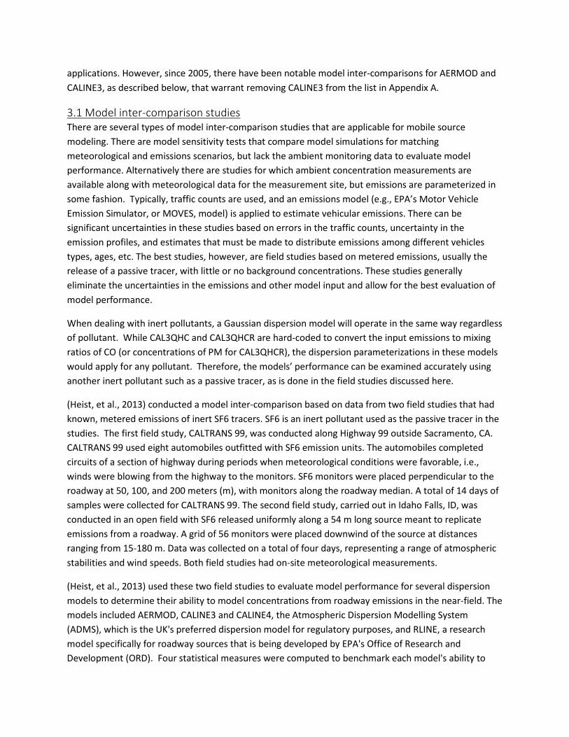
Table 1 - Model Performance Statistics from the Idaho Falls Study. Source: (Heist, et al., 2013).

Model FB (0 is best) NMSE (0 is best) R (1 is best) FAC2 (1 is best)

CALINE4 0.42 1.94 0.76 0.59

AERMOD - volume 0.38 1.26 0.84 0.59

AERMOD - area 0.32 1.25 0.82 0.59

ADMS 0.36 1.14 0.88 0.70

RLINE 0.23 0.96 0.85 0.73

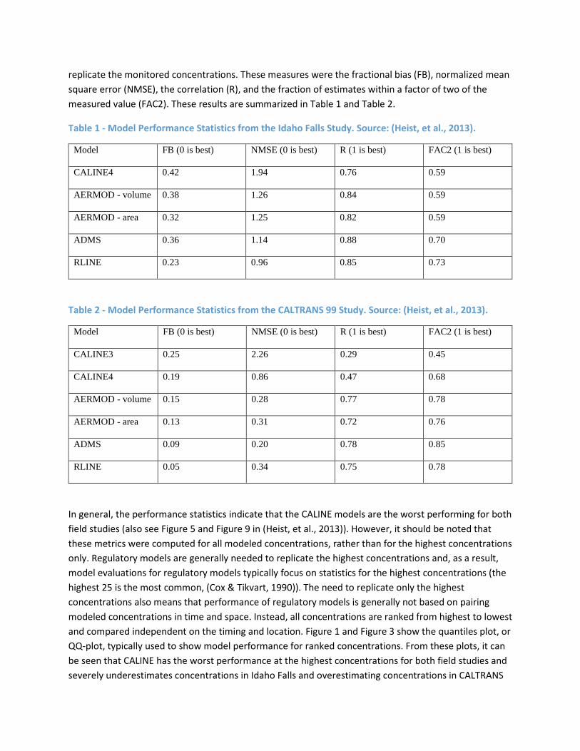
Table 2 - Model Performance Statistics from the CALTRANS 99 Study. Source: (Heist, et al., 2013).

Model FB (0 is best) NMSE (0 is best) R (1 is best) FAC2 (1 is best)

CALINE3 0.25 2.26 0.29 0.45

CALINE4 0.19 0.86 0.47 0.68

AERMOD - volume 0.15 0.28 0.77 0.78

AERMOD - area 0.13 0.31 0.72 0.76

ADMS 0.09 0.20 0.78 0.85

RLINE 0.05 0.34 0.75 0.78

In general, the performance statistics indicate that the CALINE models are the worst performing for both field studies (also see Figure 5 and Figure 9 in (Heist, et al., 2013)). However, it should be noted that these metrics were computed for all modeled concentrations, rather than for the highest concentrations only. Regulatory models are generally needed to replicate the highest concentrations and, as a result, model evaluations for regulatory models typically focus on statistics for the highest concentrations (the highest 25 is the most common, (Cox & Tikvart, 1990)). The need to replicate only the highest concentrations also means that performance of regulatory models is generally not based on pairing modeled concentrations in time and space. Instead, all concentrations are ranked from highest to lowest and compared independent on the timing and location. Figure 1 and Figure 3 show the quantiles plot, or QQ-plot, typically used to show model performance for ranked concentrations. From these plots, it can be seen that CALINE has the worst performance at the highest concentrations for both field studies and severely underestimates concentrations in Idaho Falls and overestimating concentrations in CALTRANS

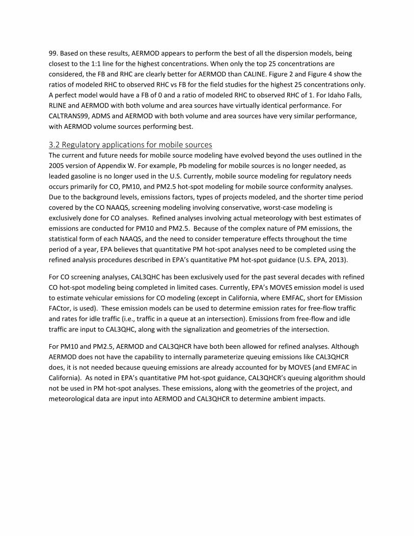
99. Based on these results, AERMOD appears to perform the best of all the dispersion models, being closest to the 1:1 line for the highest concentrations. When only the top 25 concentrations are considered, the FB and RHC are clearly better for AERMOD than CALINE. Figure 2 and Figure 4 show the ratios of modeled RHC to observed RHC vs FB for the field studies for the highest 25 concentrations only. A perfect model would have a FB of 0 and a ratio of modeled RHC to observed RHC of 1. For Idaho Falls, RLINE and AERMOD with both volume and area sources have virtually identical performance. For CALTRANS99, ADMS and AERMOD with both volume and area sources have very similar performance, with AERMOD volume sources performing best.

3.2 Regulatory applications for mobile sources The current and future needs for mobile source modeling have evolved beyond the uses outlined in the 2005 version of Appendix W. For example, Pb modeling for mobile sources is no longer needed, as leaded gasoline is no longer used in the U.S. Currently, mobile source modeling for regulatory needs occurs primarily for CO, PM10, and PM2.5 hot-spot modeling for mobile source conformity analyses. Due to the background levels, emissions factors, types of projects modeled, and the shorter time period covered by the CO NAAQS, screening modeling involving conservative, worst-case modeling is exclusively done for CO analyses. Refined analyses involving actual meteorology with best estimates of emissions are conducted for PM10 and PM2.5. Because of the complex nature of PM emissions, the statistical form of each NAAQS, and the need to consider temperature effects throughout the time period of a year, EPA believes that quantitative PM hot-spot analyses need to be completed using the refined analysis procedures described in EPA’s quantitative PM hot-spot guidance (U.S. EPA, 2013).

For CO screening analyses, CAL3QHC has been exclusively used for the past several decades with refined CO hot-spot modeling being completed in limited cases. Currently, EPA’s MOVES emission model is used to estimate vehicular emissions for CO modeling (except in California, where EMFAC, short for EMission FACtor, is used). These emission models can be used to determine emission rates for free-flow traffic and rates for idle traffic (i.e., traffic in a queue at an intersection). Emissions from free-flow and idle traffic are input to CAL3QHC, along with the signalization and geometries of the intersection.

For PM10 and PM2.5, AERMOD and CAL3QHCR have both been allowed for refined analyses. Although AERMOD does not have the capability to internally parameterize queuing emissions like CAL3QHCR does, it is not needed because queuing emissions are already accounted for by MOVES (and EMFAC in California). As noted in EPA’s quantitative PM hot-spot guidance, CAL3QHCR’s queuing algorithm should not be used in PM hot-spot analyses. These emissions, along with the geometries of the project, and meteorological data are input into AERMOD and CAL3QHCR to determine ambient impacts.

Figure 1 - QQ plot of Model Performance for Idaho Falls Study, based on (Heist, et al., 2013).

Figure 2 - RHC vs FB Model Performance Statistics for Idaho Falls Study, based on (Heist, et al., 2013).

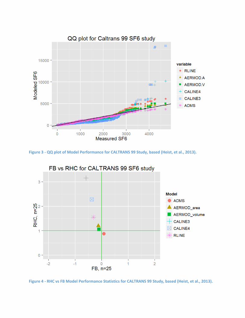
Figure 3 - QQ plot of Model Performance for CALTRANS 99 Study, based (Heist, et al., 2013).

Figure 4 - RHC vs FB Model Performance Statistics for CALTRANS 99 Study, based (Heist, et al., 2013).

3.3 Summary of findings and recommended model As discussed in section 3.1.1 of Appendix W, EPA should only list a preferred model in Appendix A when it is “found to perform better than others.” In the 2005 update to Appendix W, no comparison was made between AERMOD and CALINE3 to assess which model actually performed better for mobile source applications. However, since that time, model inter-comparison studies now provide strong evidence that AERMOD is the best performing model relative to CALINE3 (and CALINE4) for mobile source applications. Specifically, EPA has found that:

• The dispersion modeling science used in CALINE3 is very outdated (30 years old) as compared to AERMOD, RLINE and other state-of-the-science dispersion models. CALINE3 is based on the same dispersion science underlying the ISCTS3 model, which EPA replaced with AERMOD in 2005 as the preferred regulatory dispersion model for inert pollutants.

• The model performance evaluations presented by (Heist, et al., 2013) represent the best model comparison for AERMOD, CALINE3 and CALINE4 to date. This study used metered emissions of an SF6 tracer and concurrent near-road measurements to serve explicitly as a platform for evaluating mobile source models. The results showed that CALINE3 and CALINE4 were the worst performing models of the 5-model comparison for the two available field studies (Idaho Falls and CALTRANS 99) when considering all modeled and monitored concentrations, paired in time and space.

• Additional analysis of the data from (Heist, et al., 2013) was conducted by EPA in the context of regulatory use of models. This analysis focused on the highest concentrations (i.e., top 25 concentrations), which are most relevant for regulatory purposes, and typically the focus of performance evaluations of regulatory models. This additional analysis showed that not only were CALINE3 and CALINE4 the worst performers, but that AERMOD was the best performing model of the group.

• As described in more detail in Appendix A below, CALINE3 is insensitive to changes in mixing height which provides further support for the replacement of this model with AERMOD. For surface releases like roadways, low winds, stable conditions and a low mixing height are expected to result in the worst case concentrations because they are kept close to the ground. The recommendations in the 1995 CAL3QHC User’s Guide result in assumptions that are somewhat contradictory and unrealistic.

In addition to the evidence about model performance, CALINE3, CAL3QHC, and CAL3QHCR have several limitations related to the model input that make them more difficult than AERMOD to use for refined modeling:

• Meteorological pre-processors for the CALINE3 models are only available for older meteorological data sets. As a result, newer, higher resolution meteorological data, that is more representative of actual wind conditions cannot readily be used. In contrast, pre-processed meteorological data from AERMET is available from state air agencies for use in AERMOD.

• For CAL3QHCR, only 1 year of meteorological data can be used in each model run. For

refined PM10 and PM2.5 analyses, this requires multiple model runs to cover a 5-year modeling period with resulting model output data from up to 20 model runs that must be separately post-processed to obtain the necessary results.

Based on the data available, AERMOD is the best performing model for mobile source applications. Additionally, AERMOD is not limited by the practical usability issues especially in terms of most recent and improved model inputs data inputs that are not available with the CALINE3 models. As a result of these factors, EPA has proposed to replace CALINE3 with AERMOD for all mobile source applications. This proposed change also promotes greater commonality and consistency in air quality modeling analyses for EPA regulatory applications. For mobile sources, regulatory situations in which AERMOD would be used now and in future include:

• PM hot-spot analyses • CO hot-spot analyses • PM SIP attainment demonstrations • PSD applications (PM, SO2, NO2, Pb, CO) • NO2 near-road monitor siting and other potential future applications

4. Acknowledgements The authors would like to acknowledge the intra-agency workgroup, specifically contributions from staff in the Office of Research and Development, the Office of Transportation and Air Quality, and Regions 5 and 8.

5. Additional information Data for the analyses presented in this TSD can be obtained by contacting:

Chris Owen, PhD Office of Air Quality Planning and Standards, U. S. EPA 109 T.W. Alexander Dr. RTP, NC 27711 919-541-5312 owen.chris@epa.gov

References Benson, P. (1979). CALINE3--a versatile dispersion model for predicting air pollutant levels near highways

and arterial streets. FHWA-CA-TL-79-23: CA DOT, Sacramento, CO.

Benson, P. (1984). CALINE4--a dispersion model for predicting air pollutant concentrations near roadways. California Department of Transportation, Sacramento, CA: FHWA-CA-TL-84-15.

Benson, P. (1992). A review of the development and application of the CALINE3 and CALINE4 models. Atm. Env., 379-390.

Cimorelli, et al. (2005). AERMOD: A Dispersion Model for Industrial Source Applications. Part I: General Model Formulation and Boundary Layer Characterization. J. App. Meterol., 682-693.

Cox, W., & Tikvart, J. (1990). A Statistical Procedure for Determining the Best Performing Air Quality Simulation Model. Atmos. Environ., 24, 2387–2395.

Eckhoff, P., & Braverman, T. (1995). Addendum to the User's Guide to CAL3QHC Version 2.0 (CAL3QHCR User's Guide). OAQPS, RTP, NC.

Hartley, W., Carr, E., & Bailey, C. (2006). Modeling hotspot transportation-related air quality impacts using ISC, AERMOD, and HYROAD. Proceedings of Air & Waste Management Association Specialty Conference on Air Quality Models. .

Heist, et al. (2013). Estimating near-road pollutant dispersion: A model inter-comparison. Trans. Res. Part D, 93-105.

Perry, et al. (2005). AERMOD: A Dispersion Model for Industrial Source Applications. Part II: Model Performance against 17 Field Study Databases. J. App. Meterol., 694-708.

U. S. EPA. (1992). Guideline for Modeling Carbon Monoxide from Roadway Intersections, EPA document number EPA-454/R-92-005. Research Triangle Park, NC: Office of Air Quality Planning and Standards.

U. S. EPA. (1995). User's guide to CAL3QHC version 2.0: A modeling methodology for predicting pollutant concentrations near roadway intersections (revised). OAQPS, RTP, NC: EPA-454/R-92-006R.

U. S. EPA. (2008). Risk and Exposure Assessment to Support the Review of the NO2 Primary National Ambient Air Quality Standard, EPA document # EPA-452/R-08-008a. RTP, NC.

U. S. EPA. (2011). AERSCREEN User’s Guide. RTP, NC 27711, EPA-454/B-11-001: Office of Air Quality Planning and Standards.

U.S. EPA. (2013). Transportation Conformity Guidance for Quantitative Hot-Spot Analyses in PM2.5 and PM10 Nonattainment and Maintenance Areas . Retrieved from Transportation and Climate Division, Office of Transportation and Air Quality, EPA-420-B-13-053.

Appendix A Results from comparison of AERMOD and CAL3QHC for CO hot-spot screening for highway and intersection projects As noted main document, AERMOD is already used for PM10 and PM2.5 hot-spot analyses. However, for CO hot-spot analyses, CAL3QHC is currently the primary air quality model used. Therefore, some comparisons of CO screening scenarios are presented here to illustrate the differences between AERMOD and CAL3QHC for these types of analyses and to illustrate how AERMOD can be used for CO screening purposes in hot-spot analyses.

The basis for these comparisons is modeled emissions from a simple one-mile highway segment, consisting of four lanes, two in the northbound and two in the southbound directions. MOVES2014 was used at the project scale to estimate emissions from this roadway in the year 2015. Runs were done in both the Inventory mode to produce total CO emissions in the hour, and in the Emission Rates mode to produce a CO rate per vehicle-mile. The following choices were made in MOVES:

• Each lane was assumed to have 2000 vehicles traveling during the hour, i.e., 4000 vehicles in each direction per hour, for both the highway and the arterial. This amount of vehicles is close to capacity for the length of road, to be conservative (i.e., produce a higher level of emissions).

• A temperature of -10˚F and humidity of 50% was assumed, to be conservative because CO emissions increase at colder temperatures.

• The average speed on the highway was assumed to be 74 mph. • All valid combinations of gasoline, diesel, ethanol, and CNG capable vehicles were chosen, and

EPA used a typical mix of vehicles for each facility type. • The age distribution of vehicles was based on EPA’s age distribution calculator (default

information), for 2015. • No I/M program was assumed. • Default fuel parameters for Washtenaw County, Michigan were used.

MOVES2014 produced the following emissions:

Table 3 - Summary of MOVES emissions for CO example

Vehicle type Highway emissions, each direction (i.e., two lanes) Heavy duty vehicles 1791 g (10.2 %) Light duty vehicles 15,747 g (89.8%) Total 17,538 g

For the air quality modeling, the following combinations of source characteristics were included:

• Urban Dispersion (urban population of 1,000,000 used in AERMOD) • Free Flow Lanes, At Grade (TYP=AG) • 4 Lanes, (2 north bound lanes, 2 south bound lanes) • Lane Width = 12 ft (3.66 m), Lane Length = 5280 ft (1 mile) • Surface Roughness = 0.01 m • Highway: 10.2% emissions from heavy duty vehicles, 89.8% from light duty vehicles

• 36 wind directions modeled, every 10 degrees

There are several settings that are unique to each model, in particular AERMOD has more source-characterizations options than CAL3QHC. The model-specific settings are summarized as follows:

• CAL3QHC o Link Type = At Grade o Link Width = (# lanes X 12 ft) + 20 ft, i.e. 4 x 12 +20 ft = 68 ft o Link Height = 0 ft

• AERMOD: o Each link modeled as a single LINE source o Source Elevation = 0 m o LINE Width = (# lanes X 3.66 m) + 6 m, i.e. 4 x 3.66 + 6 = 20.64 m, or 67.72 ft o Release Height: based on weighted emissions by vehicle mix o Vertical Dispersion Coefficient: based on weighted emissions by vehicle mix

The source characterization for AERMOD was modified to meet recommendations outlined for PM hot-spot modeling (e.g., source width and initial dispersion parameters, σv and σz). The full details of the source characteristics and receptor locations are given in Table 3, Table 4, Table 5, and Table 6. Receptors were placed at a height of = 1.83 m (6 ft) for both models.

CAL3QHC is used for screening analyses which focuses on using "worst-case" meteorology to estimate the worst possible 1-hour concentrations. For the examples provided here, the “worst case” meteorology was taken from the original CAL3QHC runs, which consists of a 1000 m mixing height, a 1 m/s wind speed and high stabilty (P-G stability class 5). The selection of this meteorological combination is consistent with the CAL3QHC User Guide and EPA’s current guidance for CO screening analyses (U. S. EPA, 1992). However, these assumptions are somewhat contradictory and unrealistic. For surface releases like roadways, low winds, stable conditions and a low mixing height are expected to result in the worst case concentrations because emissions are kept close to the ground. These conditions typically occur during nighttime, as mixing heights and turbulence are generally higher and during the day due to solar heating of the surface. The mixing height of 1000 m used in this scenario is much too high for “worst case” concentrations and in fact could not physically occur in the atmosphere with the accompanying low wind and highly stable conditions. Despite this, the 1000 m mixing height is recommended in the 1995 CAL3QHC User’s Guide:

“Mixing height should be generally set at 1000 m. CALINE-3 sensitivity to mixing height is significant only for extremely low values (much less than 100 m).”

(As noted above, the fact that CALINE3 is insensitive to changes to the mixing height provides further support for the replacement of this model with AERMOD.) Despite the unrealistic meteorological conditions used in the CAL3QHC, they were replicated as closely as possible for the base case in AERMOD. The AERMOD meteorology was created using the MAKEMET tool provided with AERSCREEN (U. S. EPA, 2011) to find met conditions corresponding to the CAL3QHC “worst-case” stability and mixing height. These met scenarios corresponded to wind speeds of 10 m/s. The 10 m/s winds were then replaced with 1 m/s to approximately match the CAL3QHC “worst-case”.

In addition to the CAL3QHC “worst-case” scenario, several additional meteorological scenarios were created with MAKEMET that were then, as closely as possible, converted to equivalent meteorology for use in CAL3QHC. In the first case, the unsubstituted wind-speed meteorology from the “worst-case” was used, evaluating a stable condition, with high wind speeds and a high mixing height. The other scenarios are meant to represent a range of meteorological conditions, including representative nighttime meteorology, with low mixing height, wind speeds, and high stability (a closer representation of the “worst-case”), and a moderately unstable daytime condition, with moderate wind speeds and mixing heights. In contrast to the base case meteorology, the meteorology generated with MAKEMET are meteorological conditions that could actually be observed in the atmosphere. The additional meteorological scenarios also highlight how responsive AERMOD is relative to CAL3QHC.

The results from these tests are shown in Table 7. For the base (and unrealistic) case, AERMOD has lower concentrations than CAL3QHC. For the other scenarios, AERMOD has higher concentrations. As shown in the results above, in some cases CALINE3 will underpredict, while in others, CALINE3 will overpredict. In contrast, AERMOD is expected to most accurately estimate concentrations. Thus, the higher concentrations predicted by AERMOD for these alternative scenarios are expected to be reasonable and more accurate than CAL3QHC.

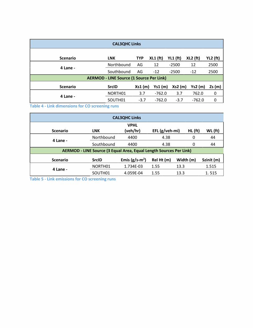
CAL3QHC Links

Scenario LNK TYP XL1 (ft) YL1 (ft) XL2 (ft) YL2 (ft)

4 Lane - Northbound AG 12 -2500 12 2500 Southbound AG -12 -2500 -12 2500

AERMOD - LINE Source (1 Source Per Link)

Scenario SrcID Xs1 (m) Ys1 (m) Xs2 (m) Ys2 (m) Zs (m)

4 Lane - NORTH01 3.7 -762.0 3.7 762.0 0 SOUTH01 -3.7 -762.0 -3.7 -762.0 0

Table 4 - Link dimensions for CO screening runs

CAL3QHC Links

Scenario LNK VPHL

(veh/hr) EFL (g/veh-mi) HL (ft) WL (ft)

4 Lane - Northbound 4400 4.38 0 44 Southbound 4400 4.38 0 44

AERMOD - LINE Source (3 Equal Area, Equal Length Sources Per Link)

Scenario SrcID Emis (g/s-m2) Rel Ht (m) Width (m) Szinit (m)

4 Lane - NORTH01 1.734E-03 1.55 13.3 1.515 SOUTH01 4.059E-04 1.55 13.3 1. 515

Table 5 - Link emissions for CO screening runs

Receptor Name X (ft) Y (ft) Z (ft) X (m) Y (m) Z (m)

REC 10R 50.40 0.00 6.00 15.36 0.00 1.83 REC 20R 60.40 0.00 6.00 18.41 0.00 1.83 REC 30R 70.40 0.00 6.00 21.46 0.00 1.83 REC 55R 95.40 0.00 6.00 29.08 0.00 1.83 REC 80R 120.40 0.00 6.00 36.70 0.00 1.83 REC 105R 145.40 0.00 6.00 44.32 0.00 1.83 REC 130R 170.40 0.00 6.00 51.94 0.00 1.83 REC 155R 195.40 0.00 6.00 59.56 0.00 1.83 REC 180R 220.40 0.00 6.00 67.18 0.00 1.83 REC 295R 335.40 0.00 6.00 102.23 0.00 1.83 REC 10L -50.40 0.00 6.00 -15.36 0.00 1.83 REC 20L -60.40 0.00 6.00 -18.41 0.00 1.83 REC 30L -70.40 0.00 6.00 -21.46 0.00 1.83 REC 55L -95.40 0.00 6.00 -29.08 0.00 1.83 REC 80L -120.40 0.00 6.00 -36.70 0.00 1.83 REC 105L -145.40 0.00 6.00 -44.32 0.00 1.83 REC 130L -170.40 0.00 6.00 -51.94 0.00 1.83 REC 155L -195.40 0.00 6.00 -59.56 0.00 1.83 REC 180L -220.40 0.00 6.00 -67.18 0.00 1.83 REC 295L -335.40 0.00 6.00 -102.23 0.00 1.83

Table 6 - Receptor locations for CO screening runs

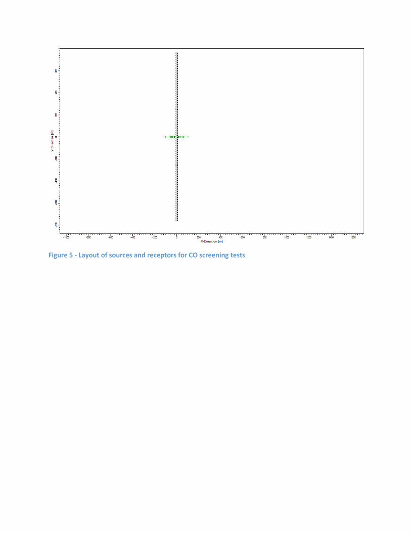
Figure 5 - Layout of sources and receptors for CO screening tests

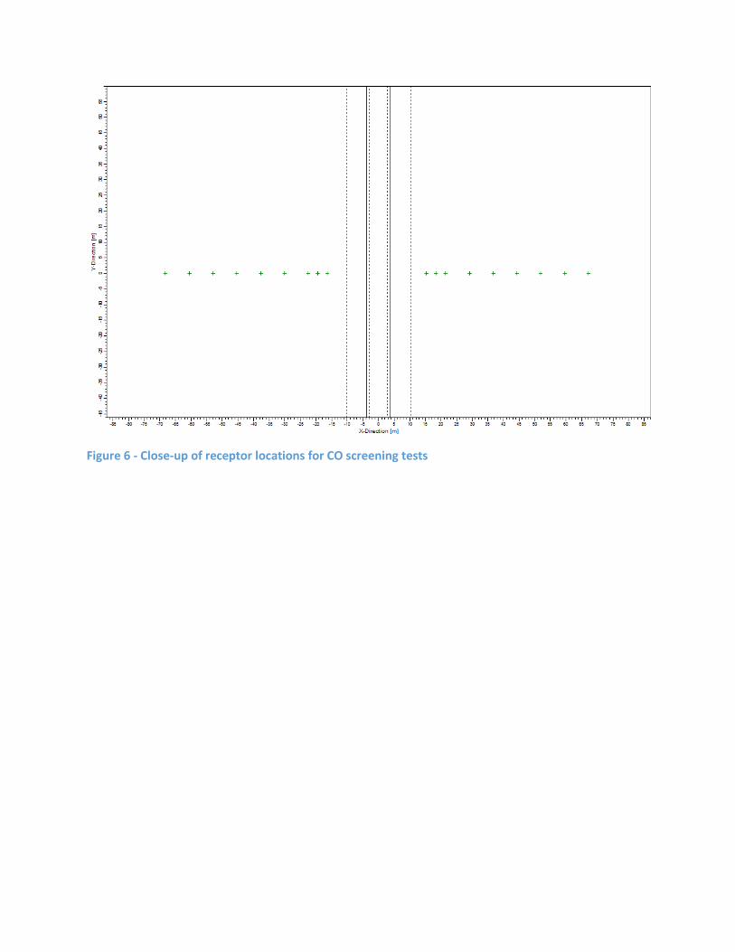
Figure 6 - Close-up of receptor locations for CO screening tests

Modeled Concentrations of CO (CAL3QHC vs. AERMOD)

Model Scenario CAL3QHC (ppm)

CAL3QHC (µg/m3)

AERMOD (µg/m3)

CAL3QHC Meteorology CAL3QHC: Mix Ht = 1000 m, Ws = 1 m/s, Stability = 5 AERMOD: Mix Ht = 992 m, Ws = 1 m/s, L = 572.5 m

2.1 2,404.5 706.0

CAL3QHC Meteorology (w/ MAKEMET Ws) CAL3QHC: Mix Ht = 1000 m, Ws = 10 m/s, Stability = 5 AERMOD: Mix Ht = 992 m, Ws = 10 m/s, L = 572.5 m

0.2 229.0 563.0

Highly Stable (Night) CAL3QHC: Mix Ht = 57 m, Ws = 1 m/s, Stability = 6 AERMOD: Mix Ht = 57 m, Ws = 1 m/s, L = 3.3 m

2.7 3,091.5 4,088.7

Moderately Unstable (Day) CAL3QHC: Mix Ht = 645 m, Ws = 2 m/s, Stability = 2 AERMOD: Mix Ht = 645 m, Ws = 2 m/s, L = -3.4 m

0.5 572.5 714.6

Table 7 - Results of CAL3QHC and AERMOD CO screening tests

United States Environmental Protection Agency

Office of Air Quality Planning and Standards Air Quality Analysis Division Research Triangle Park, NC

Publication No. EPA- 454/B-15-002 [July, 2015]