Technical Support Document (TSD) Preparation of Emissions Inventories for the 2016v1 North American Emissions Modeling Platform March 2021 Contacts: Alison Eyth, Jeff Vukovich, Caroline Farkas U.S. Environmental Protection Agency Office of Air Quality Planning and Standards Air Quality Assessment Division Emissions Inventory and Analysis Group Research Triangle Park, North Carolina
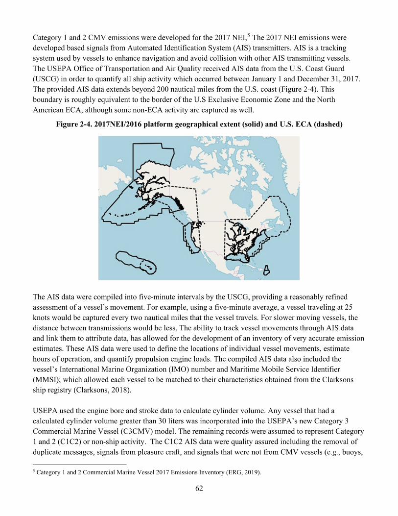
Transcript
Technical Support Document (TSD)
Preparation of Emissions Inventories for the 2016v1 North American
Emissions Modeling Platform
March 2021
Contacts: Alison Eyth, Jeff Vukovich, Caroline Farkas U.S. Environmental Protection Agency Office of Air Quality Planning and Standards Air Quality Assessment Division Emissions Inventory and Analysis Group Research Triangle Park, North Carolina
ii
TABLE OF CONTENTS LIST OF TABLES .................................................................................................................................. IV
LIST OF FIGURES ............................................................................................................................... VII
LIST OF APPENDICES ..................................................................................................................... VIII
ACRONYMS ........................................................................................................................................... IX
2.6 2016 BIOGENIC SOURCES (BEIS) ................................................................................................................................... 93 2.7 SOURCES OUTSIDE OF THE UNITED STATES.................................................................................................................. 95
2.7.1 Point Sources in Canada and Mexico (othpt) .................................................................................................... 95 2.7.2 Fugitive Dust Sources in Canada (othafdust, othptdust) ................................................................................... 95 2.7.3 Nonpoint and Nonroad Sources in Canada and Mexico (othar) ........................................................................ 96 2.7.4 Onroad Sources in Canada and Mexico (onroad_can, onroad_mex) ................................................................ 96 2.7.5 Fires in Canada and Mexico (ptfire_othna) ....................................................................................................... 96 2.7.6 Ocean Chlorine .................................................................................................................................................. 96
3.2.1 VOC speciation ................................................................................................................................................ 104 3.2.1.1 County specific profile combinations ............................................................................................................................ 107 3.2.1.2 Additional sector specific considerations for integrating HAP emissions from inventories into speciation .................. 108 3.2.1.3 Oil and gas related speciation profiles ........................................................................................................................... 111 3.2.1.4 Mobile source related VOC speciation profiles ............................................................................................................. 112
3.2.2 PM speciation................................................................................................................................................... 117 3.2.2.1 Mobile source related PM2.5 speciation profiles ........................................................................................................... 118
3.3 TEMPORAL ALLOCATION ............................................................................................................................................ 122 3.3.1 Use of FF10 format for finer than annual emissions ....................................................................................... 123 3.3.2 Electric Generating Utility temporal allocation (ptegu) .................................................................................. 124
3.3.2.1 Base year temporal allocation of EGUs ......................................................................................................................... 124
3.4 SPATIAL ALLOCATION ................................................................................................................................................ 149 3.4.1 Spatial Surrogates for U.S. emissions .............................................................................................................. 149 3.4.2 Allocation method for airport-related sources in the U.S. ............................................................................... 155 3.4.3 Surrogates for Canada and Mexico emission inventories ................................................................................ 155
3.5 PREPARATION OF EMISSIONS FOR THE CAMX MODEL ................................................................................................ 159 3.5.1 Development of CAMx Emissions for Standard CAMx Runs ........................................................................... 159 3.5.2 Development of CAMx Emissions for Source Apportionment CAMx Runs ...................................................... 161
4 DEVELOPMENT OF FUTURE YEAR EMISSIONS .............................................................. 165
4.1 EGU POINT SOURCE PROJECTIONS (PTEGU) ............................................................................................................... 169 4.2 NON-EGU POINT AND NONPOINT SECTOR PROJECTIONS ........................................................................................... 172
List of Tables Table 2-1. Platform sectors for the 2016 emissions modeling case ................................................................ 16 Table 2-2. Point source oil and gas sector NAICS Codes ................................................................................ 22 Table 2-3. 2014NEIv2-to-2016 projection factors for pt_oilgas sector for 2016v1 inventory ........................ 23 Table 2-4. 2016fh pt_oilgas national emissions (excluding offshore) before and after 2014-to-2016
projections (tons/year) .............................................................................................................................. 24 Table 2-5. Pennsylvania emissions changes for natural gas transmission sources (tons/year). ....................... 24 Table 2-6. SCCs for Census-based growth from 2014 to 2016 ........................................................................ 25 Table 2-7. 2016v1 platform SCCs for the airports sector ............................................................................... 28 Table 2-8. Afdust sector SCCs ......................................................................................................................... 29 Table 2-9. Total impact of fugitive dust adjustments to unadjusted 2016 v1 inventory ................................. 33 Table 2-10. 2016v1 platform SCCs for the ag sector ...................................................................................... 36 Table 2-11. National back-projection factors for livestock: 2017 to 2016 ...................................................... 37 Table 2-12. Source of input variables for EPIC .............................................................................................. 40 Table 2-13. 2014NEIv2-to-2016 oil and gas projection factors for CO and OK. ............................................ 42 Table 2-14. 2016 v1 platform SCCs for RWC sector ...................................................................................... 43 Table 2-15. Projection factors for RWC by SCC ............................................................................................. 44 Table 2-16. 2016v1 platform SCCs for Census-based growth ......................................................................... 46 Table 2-17. MOVES vehicle (source) types ..................................................................................................... 48 Table 2-18. Submitted data used to prepare onroad activity data .................................................................... 49 Table 2-19. Factors applied to project VMT from 2014 to 2016 to prepare default activity data ................... 50 Table 2-20. Older Vehicle Adjustments Showing the Fraction of IHS Vehicle Populations to Retain for
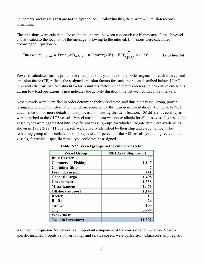
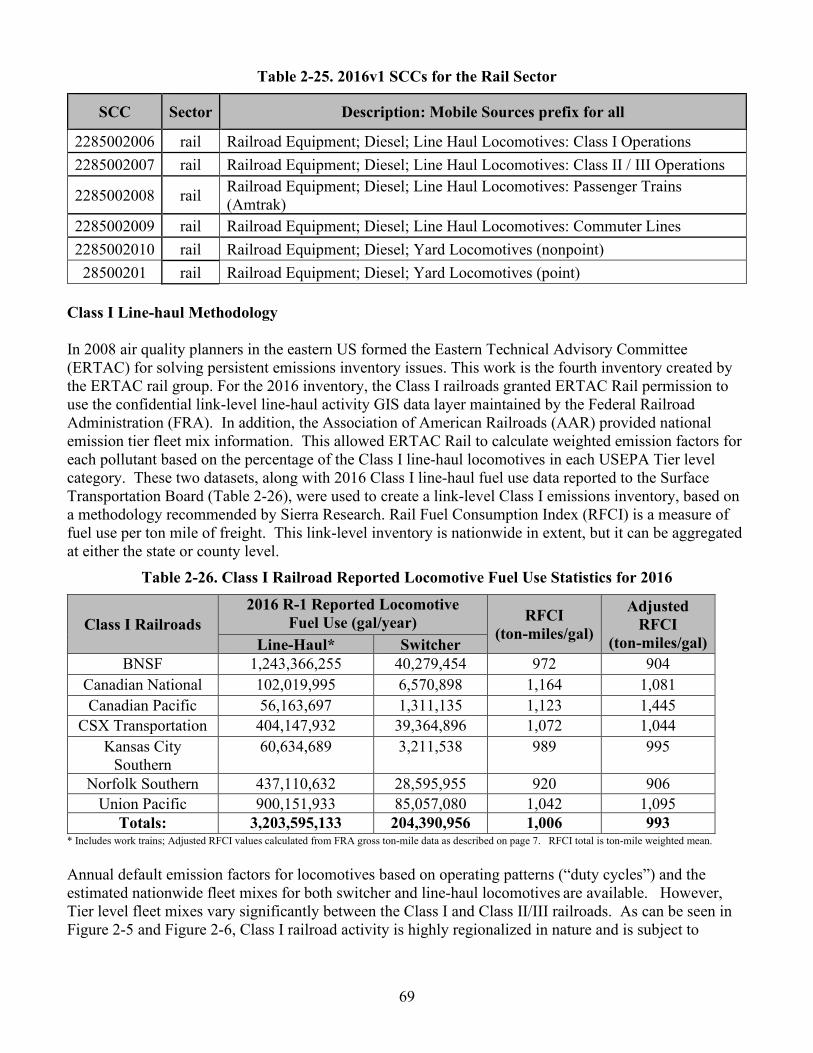
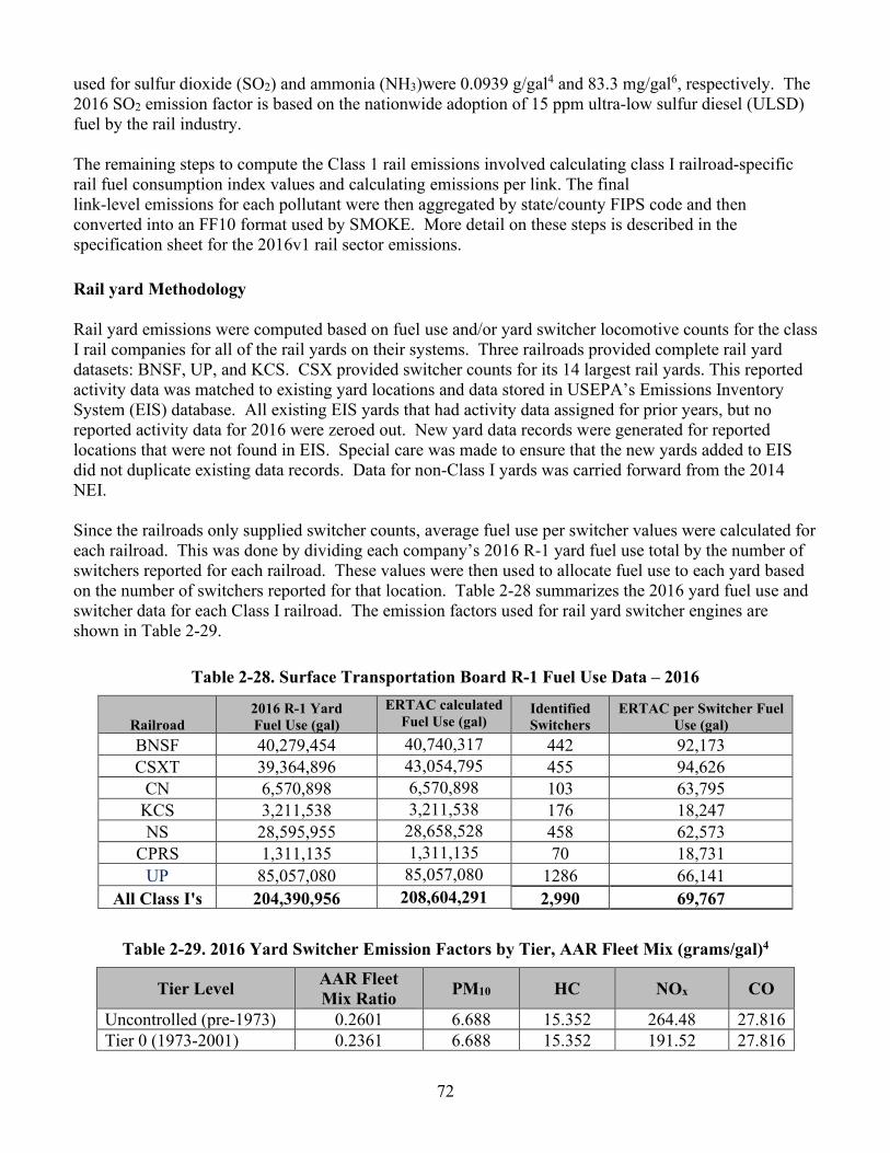
2016v1 and 2017 NEI ............................................................................................................................... 58 Table 2-21. 2016v1 platform SCCs for cmv_c1c2 sector ................................................................................ 61 Table 2-22. Vessel groups in the cmv_c1c2 sector .......................................................................................... 63 Table 2-23. 2016v1 platform SCCs for cmv_c3 sector .................................................................................... 65 Table 2-24. 2017 to 2016 projection factors for C3 CMV ............................................................................... 68 Table 2-25. 2016v1 SCCs for the Rail Sector .................................................................................................. 69 Table 2-26. Class I Railroad Reported Locomotive Fuel Use Statistics for 2016 ........................................... 69 Table 2-27. 2016 Line-haul Locomotive Emission Factors by Tier, AAR Fleet Mix (grams/gal) .................. 71 Table 2-28. Surface Transportation Board R-1 Fuel Use Data – 2016 ............................................................ 72 Table 2-29. 2016 Yard Switcher Emission Factors by Tier, AAR Fleet Mix (grams/gal)4 ............................. 72 Table 2-30. Expenditures and fuel use for commuter rail ................................................................................ 75 Table 2-31. Submitted nonroad input tables by agency ................................................................................... 81 Table 2-32. Alaska counties/census areas for which nonroad equipment sector-specific emissions are
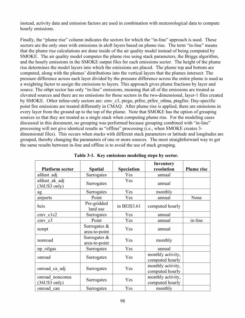
removed in 2016v1 ................................................................................................................................... 82 Table 2-33. SCCs included in the ptfire sector for the 2016v1 inventory ........................................................ 83 Table 2-34. National fire information databases used in 2016v1 ptfire inventory ........................................... 84 Table 2-35. List of S/L/T agencies that submitted fire data for 2016v1 with types and formats. .................... 86 Table 2-36. Brief description of fire information submitted for 2016v1 inventory use. .................................. 86 Table 2-37. SCCs included in the ptagfire sector for the 2016v1 inventory .................................................... 90 Table 2-38. Assumed field size of agricultural fires per state(acres) ............................................................... 92 Table 2-39. Hourly Meteorological variables required by BEIS 3.61 ............................................................. 94 Table 3-1. Key emissions modeling steps by sector. ....................................................................................... 98 Table 3-2. Descriptions of the platform grids ............................................................................................... 100 Table 3-3. Emission model species produced for CB6 for CMAQ ................................................................ 102 Table 3-4. Integration status of naphthalene, benzene, acetaldehyde, formaldehyde and methanol (NBAFM)
for each platform sector .......................................................................................................................... 106 Table 3-5. Ethanol percentages by volume by Canadian province ................................................................ 108
v
Table 3-6. MOVES integrated species in M-profiles .................................................................................... 109 Table 3-7. Basin/Region-specific profiles for oil and gas ............................................................................. 111 Table 3-8. TOG MOVES-SMOKE Speciation for nonroad emissions in MOVES2014a used for the 2016
Platform .................................................................................................................................................. 112 Table 3-9. Select mobile-related VOC profiles 2016 .................................................................................... 113 Table 3-10. Onroad M-profiles ...................................................................................................................... 114 Table 3-11. MOVES process IDs .................................................................................................................. 115 Table 3-12. MOVES Fuel subtype IDs ......................................................................................................... 116 Table 3-13. MOVES regclass IDs ................................................................................................................. 116 Table 3-14. SPECIATE4.5 brake and tire profiles compared to those used in the 2011v6.3 Platform ........ 119 Table 3-15. Nonroad PM2.5 profiles ............................................................................................................. 120 Table 3-16. NOX speciation profiles .............................................................................................................. 120 Table 3-17. Sulfate split factor computation ................................................................................................. 121 Table 3-18. SO2 speciation profiles ............................................................................................................... 121 Table 3-19. Temporal settings used for the platform sectors in SMOKE ..................................................... 122 Table 3-20. U.S. Surrogates available for the 2016v1 modeling platforms .................................................. 150 Table 3-21. Off-Network Mobile Source Surrogates .................................................................................... 152 Table 3-22. Spatial Surrogates for Oil and Gas Sources ............................................................................... 152 Table 3-23. Selected 2016 CAP emissions by sector for U.S. Surrogates (short tons in 12US1).................. 153 Table 3-24. Canadian Spatial Surrogates ...................................................................................................... 156 Table 3-25. CAPs Allocated to Mexican and Canadian Spatial Surrogates (short tons in 36US3) ............... 157 Table 3-26. Emission model species mappings for CMAQ and CAMx ........................................................ 160 Table 3-27. State tags for 2023fh1, 2028fh1 USSA modeling ....................................................................... 162 Table 4-1. Overview of projection methods for the 2023 and 2028 regional cases ...................................... 165 Table 4-2. EGU sector NOx emissions by State for the 2023 and 2028 regional cases ............................... 171 Table 4-3. Subset of CoST Packet Matching Hierarchy ................................................................................ 174 Table 4-4. Summary of non-EGU stationary projections subsections ........................................................... 175 Table 4-5. Reductions from all facility/unit/stack-level closures in 2016v1 .................................................. 177 Table 4-6. Increase in total afdust PM2.5 emissions from projections in 2016v1 ........................................... 178 Table 4-7. National projection factors for livestock: 2016 to 2023 and 2028 ................................................ 179 Table 4-8. National projection factors for cmv_c1c2 ..................................................................................... 180 Table 4-9. California projection factors for cmv_c1c2 .................................................................................. 180 Table 4-10. 2016-to-2023 and 2016-2028 CMV C3 projection factors outside of California ....................... 181 Table 4-11. 2016-to-2023 and 2016-2028 CMV C3 projection factors for California .................................. 181 Table 4-12. Year 2014-2017 high-level summary of national oil and gas exploration activity .................... 184 Table 4-13. EIA’s 2019 Annual Energy Outlook (AEO) tables used to project industrial sources ............... 185 Table 4-14. Assumed retirement rates and new source emission factor ratios for NSPS rules...................... 188 Table 4-15. Projection factors for RWC ......................................................................................................... 190 Table 4-16. Non-point (np_oilgas) SCCs in 2016v1 modeling platform where Oil and Gas NSPS controls
applied .................................................................................................................................................... 191 Table 4-17. Emissions reductions for np_oilgas sector due to application of Oil and Gas NSPS ................. 193 Table 4-18. Point source SCCs in pt_oilgas sector where Oil and Gas NSPS controls were applied. .......... 193 Table 4-19. VOC reductions (tons/year) for the pt_oilgas sector after application of the Oil and Gas NSPS
CONTROL packet for both future years 2023 and 2028. ...................................................................... 194 Table 4-20. SCCs and Engine Type in 2016v1 modeling platform where RICE NSPS controls applied for
nonpt and ptnonipm sectors. ................................................................................................................... 194 Table 4-21. Non-point Oil and Gas SCCs in 2016v1 modeling platform where RICE NSPS controls applied
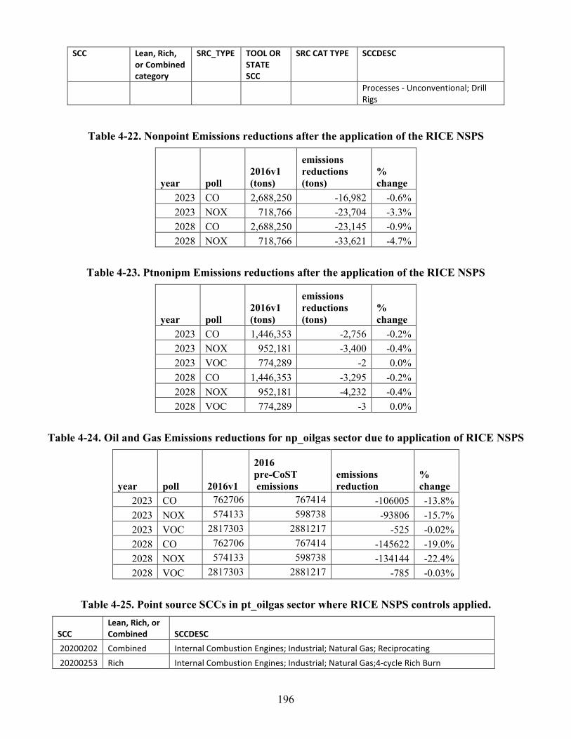
................................................................................................................................................................ 195 Table 4-22. Nonpoint Emissions reductions after the application of the RICE NSPS ................................... 196 Table 4-23. Ptnonipm Emissions reductions after the application of the RICE NSPS .................................. 196
vi
Table 4-24. Oil and Gas Emissions reductions for np_oilgas sector due to application of RICE NSPS ....... 196 Table 4-25. Point source SCCs in pt_oilgas sector where RICE NSPS controls applied. ............................. 196 Table 4-26. Emissions reductions (tons/year) in pt_oilgas sector after the application of the RICE NSPS
CONTROL packet for future years 2023 and 2028. .............................................................................. 197 Table 4-27. Summary of fuel sulfur rule impacts on nonpoint SO2 emissions for 2023 and 2028 ............... 197 Table 4-28. Summary of fuel sulfur rule impacts on ptnonipm SO2 emissions for 2023 and 2028 .............. 198 Table 4-29. Stationary gas turbines NSPS analysis and resulting emission rates used to compute controls . 198 Table 4-30. Ptnonipm SCCs in 2016v1 modeling platform where Natural Gas Turbines NSPS controls
applied .................................................................................................................................................... 199 Table 4-31. Ptnonipm emissions reductions after the application of the Natural Gas Turbines NSPS ......... 199 Table 4-32. Point source SCCs in pt_oilgas sector where Natural Gas Turbines NSPS control applied. ..... 200 Table 4-33. Emissions reductions (tons/year) for pt_oilgas after the application of the Natural Gas Turbines
NSPS CONTROL packet for future years 2023 and 2028. .................................................................... 200 Table 4-34. Process Heaters NSPS analysis and 2016v1 new emission rates used to estimate controls ....... 201 Table 4-35. Ptnonipm SCCs in 2016v1 modeling platform where Process Heaters NSPS controls applied. 201 Table 4-36. Ptnonipm emissions reductions after the application of the Process Heaters NSPS .................. 202 Table 4-37. Point source SCCs in pt_oilgas sector where Process Heaters NSPS controls were applied ..... 202 Table 4-38. NOx emissions reductions (tons/year) in pt_oilgas sector after the application of the Process
Heaters NSPS CONTROL packet for futures years 2023 and 2028. ..................................................... 203 Table 4-39. Summary of CISWI rule impacts on ptnonipm emissions for 2023 and 2028 ........................... 203 Table 4-40. Summary of NSPS Subpart JA rule impacts on ptnonipm emissions for 2023 and 2028 .......... 204 Table 4-41. Factors used to Project 2016 VMT to 2023 and 2028 ................................................................ 208 Table 4-42. Class I Line-haul Fuel Projections based on 2018 AEO Data .................................................... 209 Table 4-43. Class I Line-haul Historic and Future Year Projected Emissions ............................................... 210 Table 4-44. AEO growth rates for rail sub-groups ......................................................................................... 210 Table 4-45. Sources Added in the 2021fi Case .............................................................................................. 211 Table 5-1. National by-sector CAP emissions summaries for the 2016fh case, 12US1 grid (tons/yr) .......... 216 Table 5-2. National by-sector CAP emissions summaries for the 2023fh1 case, 12US1 grid (tons/yr) ........ 217 Table 5-3. National by-sector CAP emissions summaries for the 2028fh1 case, 12US1 grid (tons/yr) ........ 218 Table 5-4. National by-sector CAP emissions summaries for the 2016fh case, 36US3 grid (tons/yr) .......... 219 Table 5-5. National by-sector CAP emissions summaries for the 2023fh1 case, 36US3 grid (tons/yr) ........ 220 Table 5-6. National by-sector CAP emissions summaries for the 2028fh1 case, 36US3 grid (tons/yr) ........ 221 Table 5-7. National by-sector CAP emissions summaries for the 2016fi case, 12US1 grid (tons/yr) ........... 222 Table 5-8. National by-sector CAP emissions summaries for the 2021fi case, 12US1 grid (tons/yr) ........... 223 Table 5-9. National by-sector Ozone Season NOx emissions summaries 12US1 grid (tons/o.s.) ................. 224 Table 5-10. National by-sector Ozone Season VOC emissions summaries 12US1 grid (tons/o.s.) .............. 225
vii
List of Figures Figure 2-1. Impact of adjustments to fugitive dust emissions due to transport fraction, precipitation, and
cumulative ................................................................................................................................................ 35 Figure 2-2. “Bidi” modeling system used to compute 2016 Fertilizer Application emissions ........................ 39 Figure 2-3. Representative Counties in 2016v1 ............................................................................................... 60 Figure 2-4. 2017NEI/2016 platform geographical extent (solid) and U.S. ECA (dashed) .............................. 62 Figure 2-5. 2016 US Railroad Traffic Density in Millions of Gross Tons per Route Mile (MGT) ................. 70 Figure 2-6. Class I Railroads in the United States5 .......................................................................................... 70 Figure 2-7. 2016-2017 Active Rail Yard Locations in the United States ........................................................ 73 Figure 2-8. Class II and III Railroads in the United States5 ............................................................................. 74 Figure 2-9. Amtrak Routes with Diesel-powered Passenger Trains ................................................................ 76 Figure 2-10. Processing flow for fire emission estimates in the 2016v1 inventory ......................................... 88 Figure 2-11. Default fire type assignment by state and month in cases where a satellite detect is only source
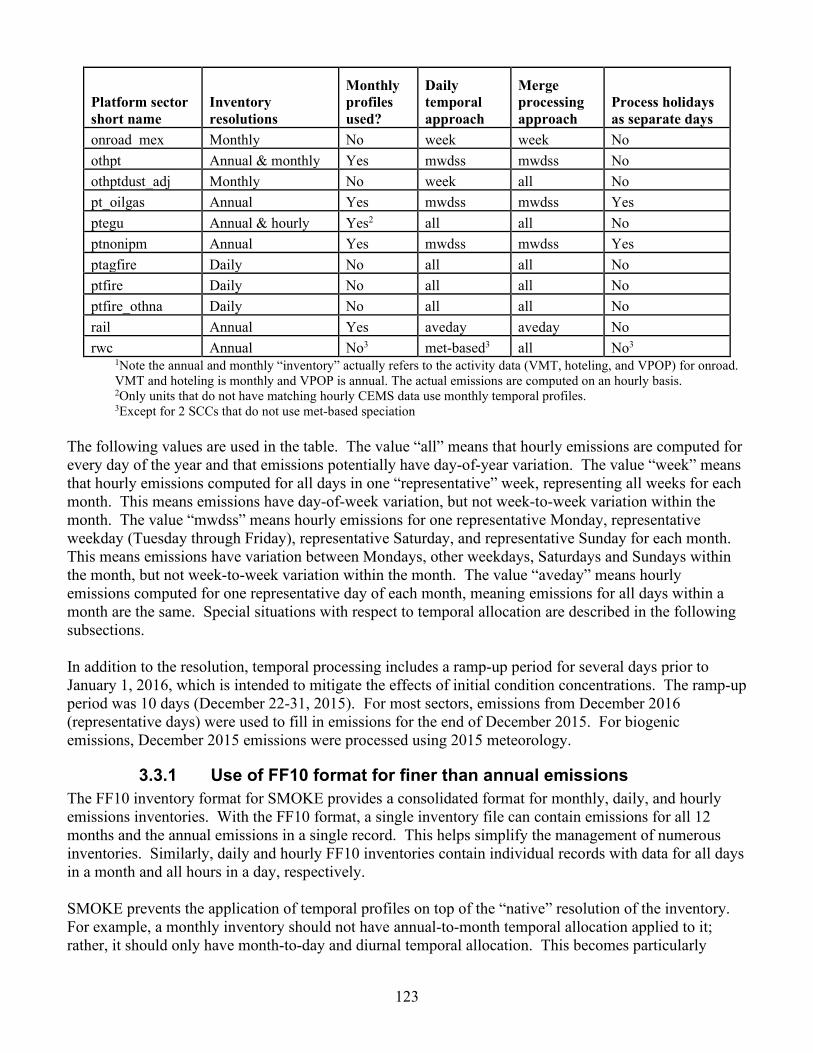
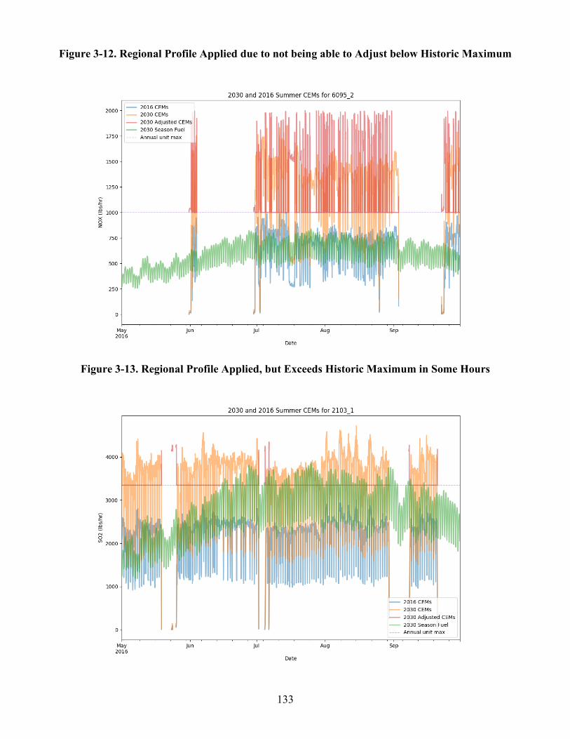
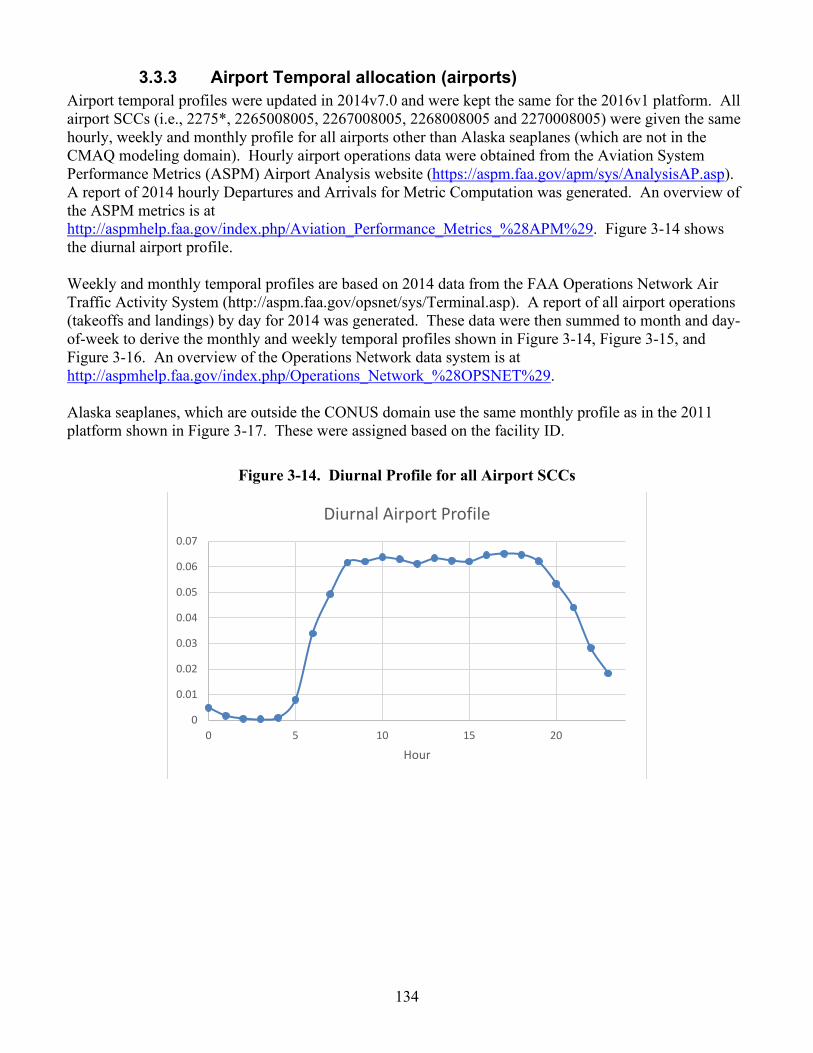
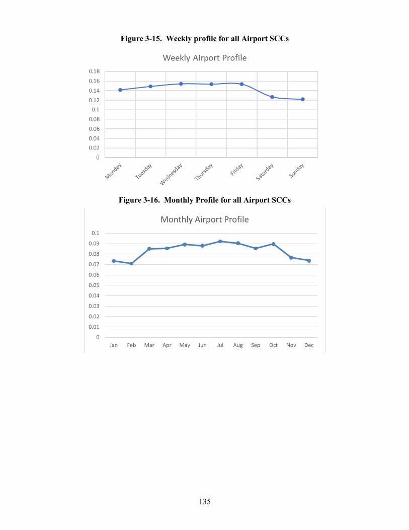
of fire information. ................................................................................................................................... 89 Figure 2-12. Blue Sky Modeling Framework .................................................................................................. 89 Figure 2-13. Normbeis3 data flows .................................................................................................................. 94 Figure 2-14. Tmpbeis3 data flow diagram. ...................................................................................................... 95 Figure 3-1. Air quality modeling domains ..................................................................................................... 100 Figure 3-2. Process of integrating NBAFM with VOC for use in VOC Speciation ...................................... 106 Figure 3-3. Profiles composited for the new PM gas combustion related sources ........................................ 117 Figure 3-4. Comparison of PM profiles used for Natural gas combustion related sources ........................... 118 Figure 3-5. Eliminating unmeasured spikes in CEMS data .......................................................................... 124 Figure 3-6. Temporal Profile Input Unit Counts by Fuel and Peaking Unit Classification .......................... 126 Figure 3-7. Example Daily Temporal Profiles for the LADCO Region and the Gas Fuel Type .................. 127 Figure 3-8. Example Diurnal Temporal Profiles for the MANE-VU Region and the Coal Fuel Type ........ 127 Figure 3-9. Non-CEMS EGU Temporal Profile Application Counts ............................................................ 128 Figure 3-10. Future Year Emissions Follow the Pattern of Base Year Emissions ......................................... 131 Figure 3-11. Excess Emissions Apportioned to Hours Less than the Historic Maximum ............................. 132 Figure 3-12. Regional Profile Applied due to not being able to Adjust below Historic Maximum............... 133 Figure 3-13. Regional Profile Applied, but Exceeds Historic Maximum in Some Hours ............................. 133 Figure 3-14. Diurnal Profile for all Airport SCCs ......................................................................................... 134 Figure 3-15. Weekly profile for all Airport SCCs ......................................................................................... 135 Figure 3-16. Monthly Profile for all Airport SCCs ....................................................................................... 135 Figure 3-17. Alaska Seaplane Profile ............................................................................................................ 136 Figure 3-18. Example of RWC temporal allocation in 2007 using a 50 versus 60 ˚F threshold .................. 137 Figure 3-19. RWC diurnal temporal profile .................................................................................................. 138 Figure 3-20. Data used to produce a diurnal profile for OHH, based on heat load (BTU/hr) ....................... 139 Figure 3-21. Day-of-week temporal profiles for OHH and Recreational RWC ........................................... 139 Figure 3-22. Annual-to-month temporal profiles for OHH and recreational RWC ...................................... 140 Figure 3-23. Example of animal NH3 emissions temporal allocation approach, summed to daily emissions
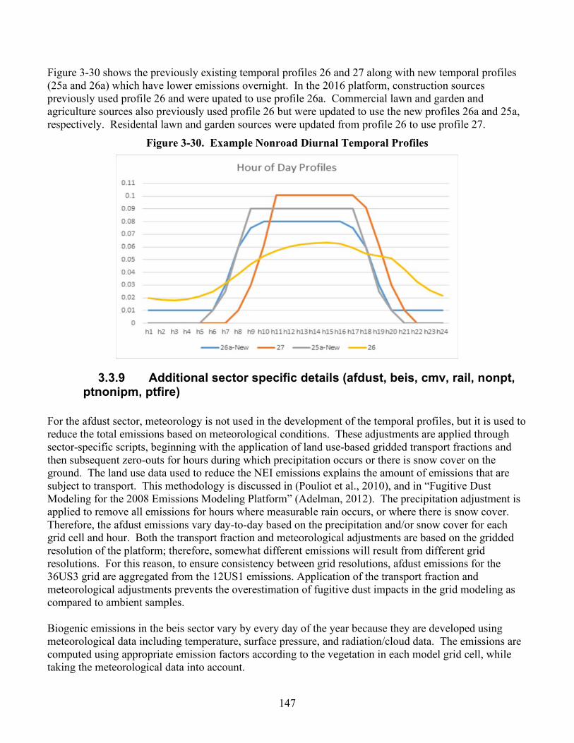
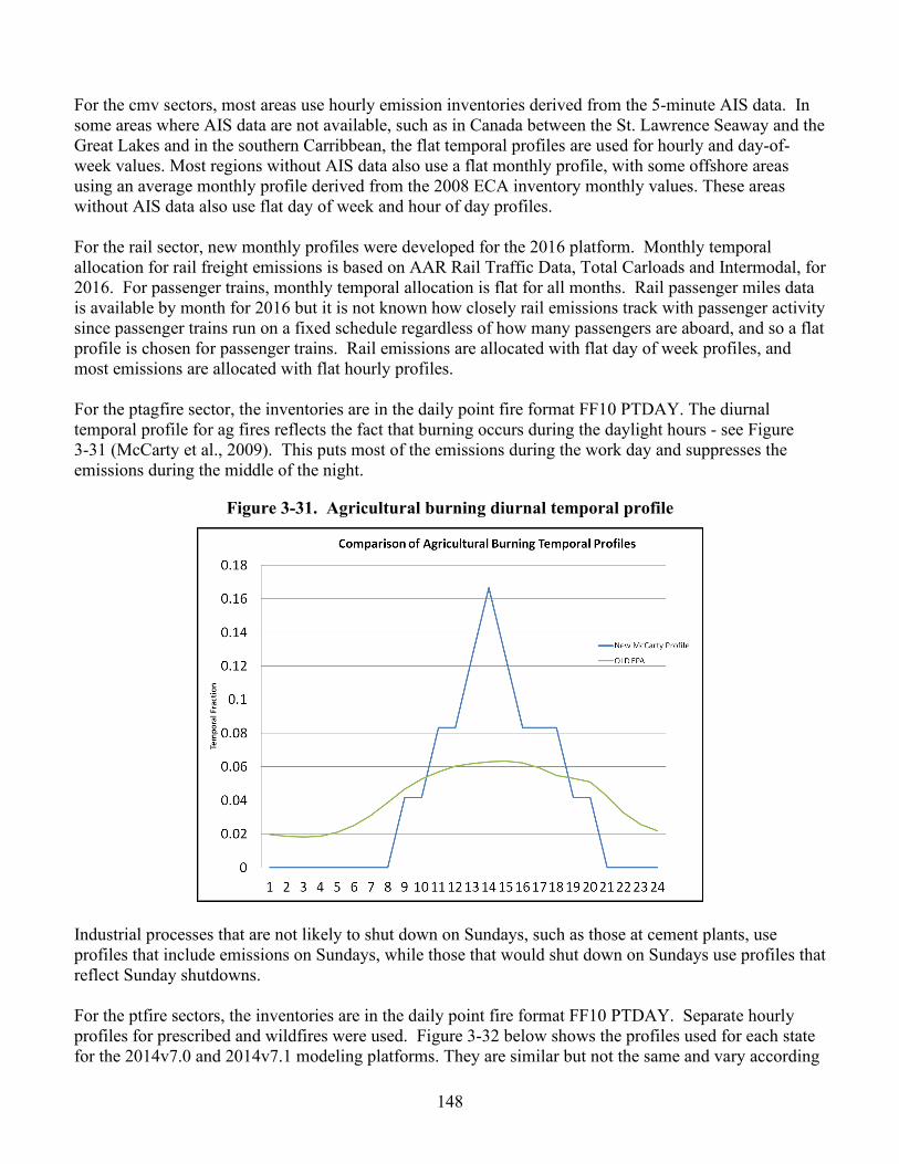
................................................................................................................................................................ 141 Figure 3-24. Example of temporal variability of NOX emissions ................................................................. 142 Figure 3-25. Sample onroad diurnal profiles for Fulton County, GA ........................................................... 143 Figure 3-26. Methods to Populate Onroad Speeds and Temporal Profiles by Road Type ........................... 144 Figure 3-27. Regions for computing Region Average Speeds and Temporal Profiles ................................. 144 Figure 3-28. Example of Temporal Profiles for Combination Trucks .......................................................... 145 Figure 3-29. Example Nonroad Day-of-week Temporal Profiles ................................................................. 146 Figure 3-30. Example Nonroad Diurnal Temporal Profiles .......................................................................... 147 Figure 3-31. Agricultural burning diurnal temporal profile .......................................................................... 148
viii
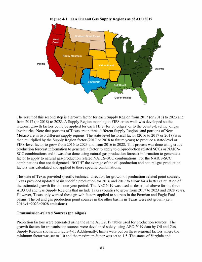
Figure 3-32. Prescribed and Wildfire diurnal temporal profiles ................................................................... 149 Figure 4-1. EIA Oil and Gas Supply Regions as of AEO2019 ..................................................................... 183
List of Appendices Appendix A: CB6 Assignment for New Species Appendix B: Profiles (other than onroad) that are new or revised in SPECIATE4.5 that were used in the
2014 v7.2 Platform Appendix C: Mapping of Fuel Distribution SCCs to BTP, BPS and RBT
ix
Acronyms AADT Annual average daily traffic AE6 CMAQ Aerosol Module, version 6, introduced in CMAQ v5.0 AEO Annual Energy Outlook AERMOD American Meteorological Society/Environmental Protection Agency
Regulatory Model AIS Automated Identification System APU Auxiliary power unit BEIS Biogenic Emissions Inventory System BELD Biogenic Emissions Land use Database BenMAP Benefits Mapping and Analysis Program BPS Bulk Plant Storage BTP Bulk Terminal (Plant) to Pump C1C2 Category 1 and 2 commercial marine vessels C3 Category 3 (commercial marine vessels) CAMD EPA’s Clean Air Markets Division CAMX Comprehensive Air Quality Model with Extensions CAP Criteria Air Pollutant CARB California Air Resources Board CB05 Carbon Bond 2005 chemical mechanism CB6 Version 6 of the Carbon Bond mechanism CBM Coal-bed methane CDB County database (input to MOVES model) CEMS Continuous Emissions Monitoring System CISWI Commercial and Industrial Solid Waste Incinerators CMAQ Community Multiscale Air Quality CMV Commercial Marine Vessel CNG Compressed natural gas CO Carbon monoxide CONUS Continental United States CoST Control Strategy Tool CRC Coordinating Research Council CSAPR Cross-State Air Pollution Rule E0, E10, E85 0%, 10% and 85% Ethanol blend gasoline, respectively ECA Emissions Control Area ECCC Environment and Climate Change Canada EF Emission Factor EGU Electric Generating Units EIA EIS
Energy Information Administration Emissions Inventory System
EPA Environmental Protection Agency EMFAC EMission FACtor (California’s onroad mobile model) EPIC Environmental Policy Integrated Climate modeling system FAA Federal Aviation Administration FCCS Fuel Characteristic Classification System FEST-C Fertilizer Emission Scenario Tool for CMAQ FF10 Flat File 2010 FINN Fire Inventory from the National Center for Atmospheric Research FIPS Federal Information Processing Standards
x
FHWA Federal Highway Administration HAP Hazardous Air Pollutant HMS Hazard Mapping System HPMS Highway Performance Monitoring System ICI Industrial/Commercial/Institutional (boilers and process heaters) I/M Inspection and Maintenance IMO International Marine Organization IPM Integrated Planning Model LADCO Lake Michigan Air Directors Consortium LDV Light-Duty Vehicle LPG Liquified Petroleum Gas MACT Maximum Achievable Control Technology MARAMA Mid-Atlantic Regional Air Management Association MATS Mercury and Air Toxics Standards MCIP Meteorology-Chemistry Interface Processor MMS Minerals Management Service (now known as the Bureau of Energy
Management, Regulation and Enforcement (BOEMRE) MOVES Motor Vehicle Emissions Simulator MSA Metropolitan Statistical Area MTBE Methyl tert-butyl ether MWC Municipal waste combustor MY Model year NAAQS National Ambient Air Quality Standards NAICS North American Industry Classification System NBAFM Naphthalene, Benzene, Acetaldehyde, Formaldehyde and Methanol NCAR National Center for Atmospheric Research NEEDS National Electric Energy Database System NEI National Emission Inventory NESCAUM Northeast States for Coordinated Air Use Management NH3 Ammonia NLCD National Land Cover Database NOAA National Oceanic and Atmospheric Administration NONROAD OTAQ’s model for estimation of nonroad mobile emissions NOX Nitrogen oxides NSPS New Source Performance Standards OHH Outdoor Hydronic Heater OTAQ EPA’s Office of Transportation and Air Quality ORIS Office of Regulatory Information System ORD EPA’s Office of Research and Development OSAT Ozone Source Apportionment Technology PFC Portable Fuel Container PM2.5 Particulate matter less than or equal to 2.5 microns PM10 Particulate matter less than or equal to 10 microns ppm arts per million ppmv Parts per million by volume PSAT Particulate Matter Source Apportionment Technology RACT Reasonably Available Control Technology RBT Refinery to Bulk Terminal RIA Regulatory Impact Analysis RICE Reciprocating Internal Combustion Engine
xi
RWC Residential Wood Combustion RPD Rate-per-vehicle (emission mode used in SMOKE-MOVES) RPH Rate-per-hour (emission mode used in SMOKE-MOVES) RPP Rate-per-profile (emission mode used in SMOKE-MOVES) RPV Rate-per-vehicle (emission mode used in SMOKE-MOVES) RVP Reid Vapor Pressure SCC Source Classification Code SMARTFIRE2 Satellite Mapping Automated Reanalysis Tool for Fire Incident Reconciliation
version 2 SMOKE Sparse Matrix Operator Kernel Emissions SO2 Sulfur dioxide SOA Secondary Organic Aerosol SIP State Implementation Plan SPDPRO S/L/T
Hourly Speed Profiles for weekday versus weekend state, local, and tribal
TAF Terminal Area Forecast TCEQ Texas Commission on Environmental Quality TOG Total Organic Gas TSD Technical support document USDA VIIRS
United States Department of Agriculture Visible Infrared Imaging Radiometer Suite
VOC Volatile organic compounds VMT Vehicle miles traveled VPOP Vehicle Population WRAP Western Regional Air Partnership WRF Weather Research and Forecasting Model 2014NEIv2 2014 National Emissions Inventory (NEI), version 2
12
1 Introduction The U.S. Environmental Protection Agency (EPA), working in conjunction with the National Emissions Inventory Collaborative, developed an air quality modeling platform for criteria air pollutants to represent the years of 2016, 2023 and 2028. The starting point for the 2016 inventory was the 2014 National Emissions Inventory (NEI), version 2 (2014NEIv2), although many inventory sectors were updated to represent the year 2016 through the incorporation of 2016-specific state and local data along with nationally-applied adjustment methods. The year 2023 and year 2028 inventories were developed starting with the 2016 inventory using sector-specific methods as described below. The inventories support several applications, including modeling in support of the Revised Cross State Air Pollution Rule (CSAPR) Update for the 2008 Ozone National Ambient Air Quality Standards (NAAQS). The air quality modeling platform consists of all the emissions inventories and ancillary data files used for emissions modeling, as well as the meteorological, initial condition, and boundary condition files needed to run the air quality model. This document focuses on the emissions modeling data and techniques including the emission inventories, the ancillary data files, and the approaches used to transform inventories for use in air quality modeling. The National Emissions Inventory Collaborative is a partnership between state emissions inventory staff, multi-jurisdictional organizations (MJOs), federal land managers (FLMs), EPA, and others to develop a North American air pollution emissions modeling platform with a base year of 2016 for use in air quality planning. The Collaborative planned for three versions of the 2016 platform: alpha, beta, and Version 1.0. This numbering format for this platform is different from previous EPA platforms which had the first number based on the version of the NEI, and the second number as a platform iteration for that NEI year (e.g., 7.3 where 7 represents 2014 NEI-based platforms, and 3 means the third iteration of the platform). For the emissions modeling documented in this technical support document (TSD), the emissions values for most sectors are the same as those in the Inventory Collaborative 2016v1 Emissions Modeling Platform, available from http://views.cira.colostate.edu/wiki/wiki/10202. In the file packages for this platform, the platform may sometimes be known as the 2016v7.3 platform. The specification sheets posted on the 2016v1 platform release page on the Wiki provide many details regarding the inventories and emissions modeling techniques in addition to those addressed in this TSD. Some updates were made to the 2016v1 platform after the fall 2019 release that were included in the Revised CSAPR Update modeling, including some minor revisions to commercial marine vessel (CMV) emissions, and electric generating unit (EGU) emissions developed in January 2020. Updates to 2016v1 to correct airport emissions and 2016 EGU processing made in June and July of 2020 were not included in the CSAPR Update modeling because the modeling was already complete by that time. The updated data and a description of them are available on the EPA FTP site ftp://newftp.epa.gov/air/emismod/2016/v1/postv1_updates/. If you cannot access the FTP site through the provided link, this link points to the same data: https://gaftp.epa.gov/Air/emismod/2016/v1/postv1_updates. This 2016 emissions modeling platform includes all criteria air pollutants (CAPs) and precursors, and a group of hazardous air pollutants (HAPs). The group of HAPs are those explicitly used by the chemical mechanism in the Community Multiscale Air Quality (CMAQ) model (Appel et al., 2018) for ozone/particulate matter (PM): chlorine (Cl), hydrogen chloride (HCl), benzene, acetaldehyde, formaldehyde, methanol, naphthalene. The modeling domain includes the lower 48 states and parts of Canada and Mexico. The modeling cases for this platform were developed for the Comprehensive Air
Quality Model with Extensions (CAMx). However, the emissions modeling process first prepares outputs in the format used by CMAQ, after which those emissions data are converted to the formats needed by CAMx. The 2016 platform used in this study consists of a 2016 base case, a 2023 case, and a 2028 case with the abbreviations 2016fh_16j, 2023fh1_16j, and 2028fh1_16j, respectively. Additional cases that included source apportionment by state and in some cases inventory sector were also developed. This platform accounts for atmospheric chemistry and transport within a state-of-the-art photochemical grid model. In the case abbreviation 2016fh_16j, 2016 is the year represented by the emissions; the “f” represents the base year emissions modeling platform iteration, which here shows that it is 2014 NEI-based (whereas for 2011 NEI-based platforms, this letter was “e”); and the “h” stands for the eighth configuration of emissions modeled for a 2014-NEI based modeling platform. The cases named 2023fh1_16j and 2028fh1_16j are the same as the original 2023fh and 2028fh future year cases, except that they include EGU emissions that were developed in January 2020 and slightly updated commercial marine vessel emissions. The case 2016fi was developed after some issues were identified with the 2016fh airport emissions inventory and with the processing of EGU emissions at specific units when multiple units in the NEI are mapped to multiple Continuous Emissions Modeling System (CEMS) units. The case 2021fi was developed to provide a representation of emissions in 2021. The 2016v1 emissions modeling platform includes point sources, nonpoint sources, commercial marine vessels (CMV), onroad and nonroad mobile sources, and fires for the U.S., Canada, and Mexico. Some platform categories use more disaggregated data than are made available in the NEI. For example, in the platform, onroad mobile source emissions are represented as hourly emissions by vehicle type, fuel type process and road type while the NEI emissions are aggregated to vehicle type/fuel type totals and annual temporal resolution. Temporal, spatial and other changes in emissions between the NEI and the emissions input into the platform are described primarily in the platform specification sheets, although a full NEI was not developed for the year 2016 because only point sources above a certain potential to emit must be submitted for years between the full triennial NEI years (e.g., 2014, 2017, 2020). Emissions from Canada and Mexico are used for the modeling platform but are not part of the NEI. The primary emissions modeling tool used to create the air quality model-ready emissions was the Sparse Matrix Operator Kernel Emissions (SMOKE) modeling system (http://www.smoke-model.org/), version 4.7 (SMOKE 4.7) with some updates. Emissions files were created for a 36-km national grid and for a 12-km national grid, both of which include the contiguous states and parts of Canada and Mexico as shown in Figure 3-1. The gridded meteorological model used to provide input data for the emissions modeling was developed using the Weather Research and Forecasting Model (WRF, https://ral.ucar.edu/solutions/products/weather-research-and-forecasting-model-wrf ) version 3.8, Advanced Research WRF core (Skamarock, et al., 2008). The WRF Model is a mesoscale numerical weather prediction system developed for both operational forecasting and atmospheric research applications. The WRF was run for 2016 over a domain covering the continental U.S. at a 12km resolution with 35 vertical layers. The run for this platform included high resolution sea surface temperature data from the Group for High Resolution Sea Surface Temperature (GHRSST) (see https://www.ghrsst.org/) and is given the EPA meteorological case label “16j.” The full case name includes this abbreviation following the emissions portion of the case name to fully specify the name of the case as “2016fh_16j.”
This document contains five sections and several appendices. Section 2 describes the 2016 inventories input to SMOKE. Section 3 describes the emissions modeling and the ancillary files used with the emission inventories. Methods to develop future year emissions are described in Section 4. Data summaries are provided in Section 5. Section 6 provides references. The Appendices provide additional details about specific technical methods or data.
15
2 Emissions Inventories and Approaches This section summarizes the emissions data that make up the 2016v1 platform. This section provides details about the data contained in each of the platform sectors for the base year and the future year. The original starting point for the emission inventories was the 2014NEIv2 although emissions for most sectors have been updated to better represent the year 2016. Documentation for the 2014NEIv2, including a TSD, is available at https://www.epa.gov/air-emissions-inventories/2014-national-emissions-inventory-nei-technical-support-document-tsd. Documentation for each 2016v1 emissions sector in the form of specification sheets is available on the 2016v1 page of Inventory Collaborative Wiki (http://views.cira.colostate.edu/wiki/wiki/10202). In addition to the NEI-based data for the broad categories of point, nonpoint, onroad, nonroad, and events (i.e., fires), emissions from the Canadian and Mexican inventories and several other non-NEI data sources are included in the 2016 platform. The triennial NEI data for CAPs are largely compiled from data submitted by state, local and tribal (S/L/T) air agencies. HAP emissions data are also from the S/L/T agencies, but, are often augmented by the EPA because they are voluntarily submitted. The EPA uses the Emissions Inventory System (EIS) to compile the NEI. The EIS includes hundreds of automated quality assurance checks to help improve data quality, and also supports tracking release point (e.g., stack) coordinates separately from facility coordinates. The EPA collaborates extensively with S/L/T agencies to ensure a high quality of data in the NEI. Using the 2014NEIv2 as a starting point, the National Inventory Collaborative worked to develop a modeling platform that more closely represents the year 2016. All emissions modeling sectors were modified in some way to better represent the year 2016 for the 2016v1 platform. The point source emission inventories for the platform include partially updated emissions to represent 2016 based on state-submitted data and adjustments to much of the remaining 2014 data to better represent 2016. Agricultural and wildland fire emissions represent the year 2016. Most nonpoint source sectors started with 2014NEIv2 emissions and were adjusted to better represent the year 2016. Fertilizer emissions, nonpoint oil and gas emissions, and onroad and nonroad mobile source emissions represent the year 2016. For CMV emissions, emissions were developed based on 2017 NEI CMV emissions and the sulfur dioxide (SO2) emissions reflect rules that reduced sulfur emissions for CMV that took effect in the year 2015. For fertilizer ammonia emissions, a 2016-specific emissions inventory is used in this platform. Nonpoint oil and gas emissions were developed using 2016-specific data for oil and gas wells and their 2016 production levels. Onroad and nonroad mobile source emissions were developed using the Motor Vehicle Emission Simulator (MOVES). Onroad emissions for the platform were developed based on emissions factors output from MOVES2014b for the year 2016, run with inputs derived from the 2014NEIv2 including activity data (e.g., vehicle miles traveled and vehicle populations) provided by state and local agencies or otherwise projected to the year 2016. MOVES2014b was also used to generate nonroad emissions because it included important updates related to nonroad engine population growth rates and spatial allocation factors. For the purposes of preparing the air quality model-ready emissions, emissions from the five NEI data categories are split into finer-grained sectors used for emissions modeling. The significance of an emissions modeling or “platform sector” is that the data are run through the SMOKE programs independently from the other sectors except for the final merge (Mrggrid). The final merge program combines the sector-specific gridded, speciated, hourly emissions together to create CMAQ-ready emission inputs. For studies that use CAMx, these CMAQ-ready emissions inputs are converted into the file formats needed by CAMx.
Table 2-1 presents an overview the sectors in the 2016 platform and how they generally relate to the 2014NEIv2 as their starting point. The platform sector abbreviations are provided in italics. These abbreviations are used in the SMOKE modeling scripts, inventory file names, and throughout the remainder of this document. Through the Collaborative workgroups, state and local agencies provided data used in the development of most sectors.
Table 2-1. Platform sectors for the 2016 emissions modeling case Platform Sector:
abbreviation NEI Data Category Description and resolution of the data input to SMOKE
EGU units: ptegu Point
Point source electric generating units (EGUs) for 2016 from the Emissions Inventory System (EIS), based on 2014NEIv2 with most sources updated to 2016. Includes some specific S/L/T updates. The inventory emissions are replaced with hourly 2016 Continuous Emissions Monitoring System (CEMS) values for nitrogen oxides (NOX) and SO2 for any units that are matched to the NEI, and other pollutants for matched units are scaled from the 2016 point inventory using CEMS heat input. Emissions for all sources not matched to CEMS data come from the raw inventory. Annual resolution for sources not matched to CEMS data, hourly for CEMS sources.
Point source oil and gas: pt_oilgas
Point
Point sources for 2016 including S/L/T updates for oil and gas production and related processes based on facilities with the following NAICS: 2111, 21111, 211111, 211112 (Oil and Gas Extraction); 213111 (Drilling Oil and Gas Wells); 213112 (Support Activities for Oil and Gas Operations); 2212, 22121, 221210 (Natural Gas Distribution); 48611, 486110 (Pipeline Transportation of Crude Oil); 4862, 48621, 486210 (Pipeline Transportation of Natural Gas). Includes offshore oil and gas platforms in the Gulf of Mexico (FIPS=85). Oil and gas point sources that were not already updated to year 2016 in the baseline inventory were projected from 2014 to 2016. Annual resolution.
Aircraft and ground support equipment: airports
Point Emissions from aircraft up to 3,000 ft elevation and emissions from ground support equipment based on 2017 NEI data. Note that these emissions were found to be overestimated in June 2020.
Remaining non-EGU point: ptnonipm
Point All 2016 point source inventory records not matched to the ptegu, airports, or pt_oilgas sectors, including updates submitted by state and local agencies. Year 2016 rail yard emissions were developed by the rail workgroup. Annual resolution.
Agricultural: ag Nonpoint
Nonpoint livestock and fertilizer application emissions. Livestock includes ammonia and other pollutants (except PM2.5) and was backcasted from a draft version of 2017NEI based on animal population data from the U.S. Department of Agriculture (USDA) National Agriculture Statistics Service Quick Stats, where available. Fertilizer includes only ammonia and is estimated for 2016 using the FEST-C model. County and monthly resolution.
Agricultural fires with point resolution: ptagfire
Nonpoint
2016 agricultural fire sources based on EPA-developed data with state updates, represented as point source day-specific emissions. They are in the nonpoint NEI data category, but in the platform, they are treated as point sources. Mostly at daily resolution with some state-submitted data at monthly resolution.
17
Platform Sector: abbreviation
NEI Data Category Description and resolution of the data input to SMOKE
Area fugitive dust: afdust Nonpoint
PM10 and PM2.5 fugitive dust sources from the 2014NEIv2 nonpoint inventory with paved road dust grown to 2016 levels; including building construction, road construction, agricultural dust, and road dust. The NEI emissions are reduced during modeling according to a transport fraction (newly computed for the 2016 beta platform) and a meteorology-based (precipitation and snow/ice cover) zero-out. Afdust emissions from the portion of Southeast Alaska inside the 36US3 domain are processed in a separate sector called ‘afdust_ak’. County and annual resolution.
Biogenic: beis Nonpoint
Year 2016, hour-specific, grid cell-specific emissions generated from the BEIS3.61 model within SMOKE, including emissions in Canada and Mexico using BELD v4.1 “water fix” land use data (including improved treatment of water grid cells).
Category 1, 2 CMV: cmv_c1c2 Nonpoint
Category 1 and category 2 (C1C2) commercial marine vessel (CMV) emissions sources backcast to 2016 from the 2017NEI using a multiplier of 0.98.emissions. Includes C1C2 emissions in U.S. state and Federal waters, and also all non-U.S. C1C2 emissions including those in Canadian waters. Gridded and hourly resolution.
Category 3 CMV: cmv_c3 Nonpoint
Category 3 (C3) CMV emissions converted to point sources based on the center of the grid cells. Includes C3 emissions in U.S. state and Federal waters, and also all non-U.S. C3 emissions including those in Canadian waters. Emissions are backcast to 2016 from 2017NEI emissions based on factors derived from U.S. Army Corps of Engineers Entrance and Clearance data and information about the ships entering the ports. Gridded and hourly resolution.
Locomotives : rail Nonpoint
Line haul rail locomotives emissions developed by the rail workgroup based on 2016 activity and emission factors. Includes freight and commuter rail emissions and incorporates state and local feedback. County and annual resolution.
Remaining nonpoint: nonpt
Nonpoint 2014NEIv2 nonpoint sources not included in other platform sectors with sources proportional to human population activity data grown to year 2016; incorporates state and local feedback. County and annual resolution.
Nonpoint source oil and gas: np_oilgas
Nonpoint 2016 nonpoint oil and gas emissions output from the NEI oil and gas tool along with state and local feedback. County and annual resolution.
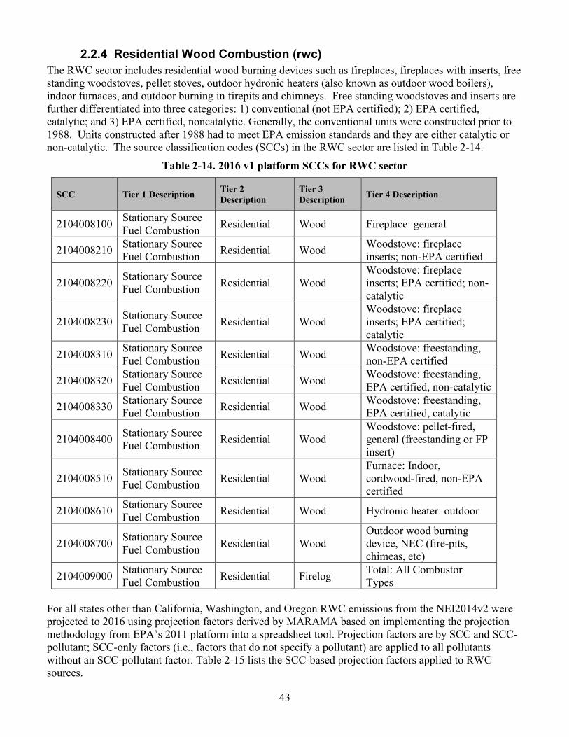
Residential Wood Combustion: rwc
Nonpoint 2014NEIv2 nonpoint sources from residential wood combustion (RWC) processes projected to the year 2016. County and annual resolution.
Nonroad: nonroad Nonroad
2016 nonroad equipment emissions developed with the MOVES2014b model which incorporates updated equipment growth rates. MOVES was used for all states except California and Texas, which submitted emissions. County and monthly resolution.
18
Platform Sector: abbreviation
NEI Data Category Description and resolution of the data input to SMOKE
Onroad: onroad Onroad
2016 onroad mobile source gasoline and diesel vehicles from moving and non-moving vehicles that drive on roads, along with vehicle refueling. Includes the following modes: exhaust, extended idle, auxiliary power units, evaporative, permeation, refueling, and brake and tire wear. For all states except California, developed using winter and summer MOVES emissions tables produced by MOVES2014b coupled with activity data projected to year 2016 or provided by S/L/T agencies. SMOKE-MOVES was used to compute emissions from the emission factors and activity data. Onroad emissions for Alaska, Hawaii, Puerto Rico and the Virgin Islands were computed using the same method as the continental U.S.,but are part of the onroad_nonconus sector.
Onroad California:
onroad_ca_adj Onroad
2016 California-provided CAP onroad mobile source gasoline and diesel vehicles based on the EMFAC model, which ere gridded and temporalized using MOVES2014b results. Volatile organic compound (VOC) HAP emissions derived from California-provided VOC emissions and MOVES-based speciation.
Point source fires- ptfire Events
Point source day-specific wildfires and prescribed fires for 2016 computed using Satellite Mapping Automated Reanalysis Tool for Fire Incident Reconciliation version 2 (SMARTFIRE2) and BlueSky Framework (Sullivan, 2008 and Raffuse, 2007) for both flaming and smoldering processes (i.e., SCCs 281XXXX002). Smoldering is forced into layer 1 (by adjusting heat flux). Incorporates state inputs. Daily resolution.
Non-US. Fires: ptfire_othna N/A
Point source day-specific wildfires and prescribed fires for 2016 provided by Environment Canada with data for missing months, and for Mexico and Central America, filled in using fires from the Fire Inventory (FINN) from National Center for Atmospheric Research (NCAR) fires (NCAR, 2016 and Wiedinmyer, C., 2011). Daily resolution.
Other Area Fugitive dust sources not from the NEI: othafdust
N/A
Fugitive dust sources of particulate matter emissions excluding land tilling from agricultural activities, from Environment and Climate Change Canada (ECCC) 2015 emission inventory, except that construction dust emissions were reduced to levels compatible with their 2010 inventory. A transport fraction adjustment is applied along with a meteorology-based (precipitation and snow/ice cover) zero-out. County and annual resolution.
Other Point Fugitive dust sources not from the NEI: othptdust
N/A
Fugitive dust sources of particulate matter emissions from land tilling from agricultural activities, ECCC 2015 emission inventory, but wind erosion emissions were removed. A transport fraction adjustment is applied along with a meteorology-based (precipitation and snow/ice cover) zero-out. Data were originally provided on a rotated 10-km grid for beta, but were smoothed so as to avoid the artifact of grid lines in the processed emissions. Monthly resolution.
19
Platform Sector: abbreviation
NEI Data Category Description and resolution of the data input to SMOKE
Other point sources not from the NEI: othpt
N/A
Point sources from the ECCC 2015 emission inventory, including agricultural ammonia, along with emissions from Mexico’s 2008 inventory projected to 2014 and 2018 and then interpolated to 2016. Agricultural data were originally provided on a rotated 10-km grid for beta, but were smoothed so as to avoid the artifact of grid lines in the processed emissions. Monthly resolution for Canada agricultural and airport emissions, annual resolution for the remainder of Canada and all of Mexico.
Other non-NEI nonpoint and nonroad: othar
N/A
Year 2015 Canada (province or sub-province resolution) emissions from the ECCC inventory: monthly for nonroad sources; annual for rail and other nonpoint Canada sectors. Year 2016 Mexico (municipio resolution) emissions, interpolated from 2014 and 2018 inventories that were projected from their 2008 inventory: annual nonpoint and nonroad mobile inventories.
Other non-NEI onroad sources: onroad_can
N/A Monthly year 2015 Canada (province resolution or sub-province resolution, depending on the province) from the ECCC onroad mobile inventory.
Other non-NEI onroad sources: onroad_mex
N/A Monthly year 2016 Mexico (municipio resolution) onroad mobile inventory based on MOVES-Mexico runs for 2014 and 2018 then interpolated to 2016.
Other natural emissions are also merged in with the above sectors: ocean chlorine and sea salt. The ocean chlorine gas emission estimates are based on the build-up of molecular chlorine (Cl2) concentrations in oceanic air masses (Bullock and Brehme, 2002). In CMAQ, the species name is “CL2”. The sea salt emissions were developed with version 4.1 of the OCEANIC pre-processor that comes with the CAMx model. The preprocessor estimates time/space-varying emissions of aerosol sodium, chloride and sulfate; gas-phase chlorine and bromine associated with sea salt; gaseous halo-methanes; and dimethyl sulfide (DMS). These additional oceanic emissions are incorporated into the final model-ready emissions files for CAMx. The emission inventories in SMOKE input formats for the platform are available from EPA’s Air Emissions Modeling website: https://www.epa.gov/air-emissions-modeling/2014-2016-version-7-air-emissions-modeling-platforms, under the section entitled “2016v1 Platform”. The platform “README” file indicates the particular zipped files associated with each platform sector. A number of reports (i.e., summaries) are available with the data files for the 2016 platform. The types of reports include state summaries of inventory pollutants and model species by modeling platform sector and county annual totals by modeling platform sector. Additional types of data including outputs from SMOKE and inputs to CAMx are available from the Intermountain West Data Warehouse.
2.1 2016 point sources (ptegu, pt_oilgas, ptnonipm, airports) Point sources are sources of emissions for which specific geographic coordinates (e.g., latitude/longitude) are specified, as in the case of an individual facility. A facility may have multiple emission release points that may be characterized as units such as boilers, reactors, spray booths, kilns, etc. A unit may have multiple processes (e.g., a boiler that sometimes burns residual oil and sometimes burns natural gas). This section describes NEI point sources within the contiguous U.S. and the offshore oil platforms which are processed by SMOKE as point source inventories. A full NEI is compiled every three years including 2011, 2014 and 2017. In the intervening years, emissions information about point sources that exceed certain potential to emit threshold are required to be submitted to the EIS that is used to compile the NEI.
A comprehensive description of how EGU emissions were characterized and estimated in the 2014 NEI is located in Section 3.4 in the 2014NEIv2 TSD. The methods for emissions estimation are similar for the interim year of 2016, but there is no TSD available specific to the 2016 point source submissions to EIS. Additional information on state submissions through the collaborative process are available in the collaborative specification sheets. The point source file used for the modeling platform is exported from EIS into the Flat File 2010 (FF10) format that is compatible with SMOKE (see https://www.cmascenter.org/smoke/documentation/4.7/html/ch08s02s08.html). For the 2016v1 platform, the export of point source emissions, including stack parameters and locations from EIS, was done on June 12, 2018. The flat file was modified to remove sources without specific locations (i.e., their FIPS code ends in 777). Then the point source FF10 was divided into four NEI-based platform point source sectors: the EGU sector (ptegu), point source oil and gas extraction-related emissions (pt_oilgas), airport emissions were put into the airports sector, and the remaining non-EGU sector also called the non-IPM (ptnonipm) sector. The split was done at the unit level for ptegu and facility level for pt_oilgas such that a facility may have units and processes in both ptnonipm and ptegu, but cannot be in both pt_oilgas and any other point sector. Additional information on updates made through the collaborative process is available in the collaborative specification sheets. The EGU emissions are split out from the other sources to facilitate the use of distinct SMOKE temporal processing and future-year projection techniques. The oil and gas sector emissions (pt_oilgas) were processed separately for summary tracking purposes and distinct future-year projection techniques from the remaining non-EGU emissions (ptnonipm). The inventory pollutants processed through SMOKE for all point source sectors were: carbon monoxide (CO), NOX, VOC, SO2, ammonia (NH3), particles less than 10 microns in diameter (PM10), and particles less than 2.5 microns in diameter (PM2.5), and all of the air toxics listed in Table 3-3. The Naphthalene, Benzene, Acetaldehyde, Formaldehyde, and Methanol (NBAFM) species are explicit in the CB6-CMAQ chemical mechanism and are taken from the HAP emissions in the flat file (if present for a source) as opposed to using emissions generated through VOC speciation, as is normally done for non-toxics modeling applications. To prevent double counting of mass, NBAFM species are removed from VOC speciation profiles, thus resulting in speciation profiles that may sum to less than 1. This is called the “no-integrate” VOC speciation case and is discussed in detail in Section 3.2.1.1. The resulting VOC in the modeling system may be higher or lower than the VOC emissions in the NEI; they would only be the same if the HAP inventory and speciation profiles were exactly consistent. For HAPs other than those in NBAFM, there is no concern for double-counting since CMAQ handles these outside the CB6 mechanism. The ptnonipm and pt_oilgas sector emissions were provided to SMOKE as annual emissions. For those ptegu sources with CEMS data that could be matched to the point inventory from EIS, hourly CEMS NOX and SO2 emissions were used rather than the annual total NEI emissions. For all other pollutants at matched units, the annual emissions were used as-is from the NEI, but were allocated to hourly values using heat input from the CEMS data. For the sources in the ptegu sector not matched to CEMS data, daily emissions were created using an approach described in Section 2.1.1. For non-CEMS units other than municipal waste combustors and cogeneration units, IPM region- and pollutant-specific diurnal profiles were applied to create hourly emissions.
2.1.1 EGU sector (ptegu) The ptegu sector contains emissions from EGUs in the 2016 NEI point inventory that could be matched to units found in the National Electric Energy Data System (NEEDS) v6 database (https://www.epa.gov/airmarkets/national-electric-energy-data-system-needs-v6). The matching was prioritized according to the amount of the emissions produced by the source. In the SMOKE point flat file, emission records for sources that have been matched to the NEEDS database have a value filled into the IPM_YN column based on the matches stored within EIS. The 2016 NEI point inventory consists of data submitted by S/L/T agencies and EPA to the EIS for Type A (i.e., large) point sources. Those EGU sources in the 2014 NEIv2 inventory that were not submitted or updated for 2016 and not identified as retired were retained. The retained 2014 NEIv2 EGUs in CT, DE, DC, ME, MD, MA, NH, NJ, NY, NC, PA, RI, VT, VA, and WV were projected from 2014 to 2016 values using factors provided by the Mid-Atlantic Regional Air Management Association (MARAMA). Higher generation capacity units in the ptegu sector are matched to 2016 CEMS data from EPA’s Clean Air Markets Division (CAMD) via ORIS facility codes and boiler ID. For the matched units, SMOKE replaces the 2016 emissions of NOX and SO2 with the CEMS emissions, thereby ignoring the annual values specified in the NEI. For other pollutants at matched units, the hourly CEMS heat input data are used to allocate the NEI annual emissions to hourly values. All stack parameters, stack locations, and Source Classification Codes (SCC) for these sources come from the NEI or updates provided by data submitters outside of EIS. Because these attributes are obtained from the NEI, the chemical speciation of VOC and PM2.5 for the sources is selected based on the SCC or in some cases, based on unit-specific data. If CEMS data exists for a unit, but the unit is not matched to the NEI, the CEMS data for that unit is not used in the modeling platform. However, if the source exists in the NEI and is not matched to a CEMS unit, the emissions from that source are still modeled using the annual emission value in the NEI temporally allocated to hourly values. The EGU flat file inventory is split into a flat file with CEMS matches and a flat file without CEMS matches to support analysis and temporalization. In the SMOKE point flat file, emission records for point sources matched to CEMS data have values filled into the ORIS_FACILITY_CODE and ORIS_BOILER_ID columns. The CEMS data in SMOKE-ready format is available at http://ampd.epa.gov/ampd/ near the bottom of the “Prepackaged Data” tab. Many smaller emitters in the CEMS program are not identified with ORIS facility or boiler IDs that can be matched to the NEI due to inconsistencies in the way a unit is defined between the NEI and CEMS datasets, or due to uncertainties in source identification such as inconsistent plant names in the two data systems. Also, the NEEDS database of units modeled by IPM includes many smaller emitting EGUs that do not have CEMS. Therefore, there will be more units in the NEEDS database than have CEMS data. The temporal allocation of EGU units matched to CEMS is based on the CEMS data, whereas regional profiles are used for most of the remaining units. More detail can be found in Section 3.3.2. Some EIS units match to multiple CAMD units based on cross-reference information in the EIS alternate identifier table. The multiple matches are used to take advantage of hourly CEMS data when a CAMD unit specific entry is not available in the inventory. Where a multiple match is made the EIS unit is split and the ORIS facility and boiler IDs are replaced with the individual CAMD unit IDs. The split EIS unit NOX and SO2 emissions annual emissions are replaced with the sum of CEMS values for that respective unit. All other pollutants are scaled from the EIS unit into the split CAMD unit using the fraction of annual heat input from the CAMD unit as part of the entire EIS unit. The NEEDS ID in the “ipm_yn” column of the flat file is updated with a “_M_” between the facility and boiler identifiers to signify that the EIS unit had multiple CEMS matches. The inventory records with multiple matches had the EIS unit identifiers appended with the ORIS boiler identifier to distinguish each CEMS record in SMOKE.
For sources not matched to CEMS data, except for municipal waste combustors (MWCs) waste-to-energy and cogeneration units, daily emissions were computed from the NEI annual emissions using average CEMS data profiles specific to fuel type, pollutant,1 and IPM region. To allocate emissions to each hour of the day, diurnal profiles were created using average CEMS data for heat input specific to fuel type and IPM region. See Section 3.3.2 for more details on the temporal allocation approach for ptegu sources. MWC and cogeneration units were specified to use uniform temporal allocation such that the emissions are allocated to constant levels for every hour of the year. These sources do not use hourly CEMs, and instead use a PTDAY file with the same emissions for each day, combined with a uniform hourly temporal profile applied by SMOKE. The ptegu inventory for the 2016fi case includes an update that allows SMOKE to properly process CEMS emissions when there are multiple CEMS units mapped to the same NEI unit. This caused NOx and SO2 emissions in 2016fi to be higher at some units.
2.1.2 Point source oil and gas sector (pt_oilgas) The pt_oilgas sector consists of point source oil and gas emissions in United States, primarily pipeline-transportation and some upstream exploration and production. Sources in the pt_oilgas sector consist of sources which are not electricity generating units (EGUs) and which have a North American Industry Classification System (NAICS) code corresponding to oil and gas exploration, production, pipeline-transportation or distribution. The pt_oilgas sector was separated from the ptnonipm sector by selecting sources with specific NAICS codes shown in Table 2-2. The use of NAICS to separate out the point oil and gas emissions forces all sources within a facility to be in this sector, as opposed to ptegu where sources within a facility can be split between ptnonipm and ptegu sectors.
Table 2-2. Point source oil and gas sector NAICS Codes
NAICS Type of point source NAICS description
2111, 21111 Production Oil and Gas Extraction 211111 Production Crude Petroleum and Natural Gas Extraction 211112 Production Natural Gas Liquid Extraction 213111 Production Drilling Oil and Gas Wells 213112 Support Support Activities for Oil and Gas Operations 2212, 22121, 221210 Distribution Natural Gas Distribution 4862, 48621, 486210 Transmission Pipeline Transportation of Natural Gas 48611, 486110 Transmission Pipeline Transportation of Crude Oil
The starting point for the 2016v1 emissions platform pt_oilgas inventory was the 2016 point source NEI. The 2016 NEI includes data submitted by S/L/T agencies and EPA to the EIS for Type A (i.e., large) point sources. Point sources in the 2014 NEIv2 not submitted for 2016 were pulled forward from the 2014 NEIv2 unless they had been marked as shut down. For the federally-owned offshore point inventory of oil and gas platforms, a 2014 inventory was developed by the U.S. Department of the Interior, Bureau of Ocean and Energy Management, Regulation, and Enforcement (BOEM).
1 The year to day profiles use NOx and SO2 CEMS for NOx and SO2, respectively. For all other pollutants, they use heat input CEMS data.
23
The 2016 pt_oilgas inventory includes sources with updated data for 2016 and sources carried forward from the 2014NEIv2 point inventory. Each type of source can be identified based on the calc_year field in the flat file 2010 (FF10) formatted inventory files, which is set to either 2016 or 2014. The pt_oilgas inventory was split into two components: one for 2016 sources, and one for 2014 sources. The 2016 sources were used in 2016v1 platform without further modification. Updates were made to selected West Virginia Type B facilities based on comments from the state. For pt_oilgas emissions that were carried forward from the 2014NEIv2, the emissions were projected to represent the year 2016. Each state/ SCC/NAICS combination in the inventory was classified as either an oil source, a natural gas source, a combination of oil and gas, or designated as a “no growth” source. Growth factors were based on historical state production data from the Energy Information Administration (EIA) and are listed in Table 2. National 2016 pt_oilgas emissions before and after application of 2014-to-2016 projections are shown in Table 3. The historical production data for years 2014 and 2016 for oil and natural gas were taken from the following websites: • https://www.eia.gov/dnav/pet/pet_crd_crpdn_adc_mbbl_a.htm (Crude production) • http://www.eia.gov/dnav/ng/ng_sum_lsum_a_epg0_fgw_mmcf_a.htm (Natural gas production) The “no growth” sources include all offshore and tribal land emissions, and all emissions with a NAICS code associated with distribution, transportation, or support activities. As there were no 2015 production data in the EIA for Idaho, no growth was assumed for this state; the only pt_oilgas sources in Idaho were pipeline transportation related. Maryland and Oregon had no oil production data on the EIA website. The factors provided in Table 2-8 were applied to sources with NAICS = 2111, 21111, 211111, 211112, and 213111 and with production-related SCC processes. Table 2-3 provides a national summary of emissions before and after this 2 year projection for these sources in the pt_oilgas sector. Table 2-4 shows the national emissions for pt_oilgas following the projection to 2016.
Table 2-3. 2014NEIv2-to-2016 projection factors for pt_oilgas sector for 2016v1 inventory
The state of Pennsylvania provided new emissions data for natural gas transmission sources for year 2016. The PA point source data replaced the emissions used in 2016beta. Table 2-5 illustrates the change in emissions with this update.
Table 2-5. Pennsylvania emissions changes for natural gas transmission sources (tons/year).
2.1.3 Non-IPM sector (ptnonipm) With minor exceptions, the ptnonipm sector contains point sources that are not in the airport, ptegu or pt_oilgas sectors. For the most part, the ptnonipm sector reflects the non-EGU sources of the NEI point inventory; however, it is likely that some small low-emitting EGUs not matched to the NEEDS database or to CEMS data are present in the ptnonipm sector. The ptnonipm emissions in the 2016v1 platform have been updated from the 2016 NEI point inventory with the following changes. Non-IPM Projection from 2014 to 2016 inside MARAMA region 2014-to-2016 projection packets for all nonpoint sources were provided by MARAMA for the following states: CT, DE, DC, ME, MD, MA, NH, NJ, NY, NC, PA, RI, VT, VA, and WV. New Jersey provided their own projection factors for projection from 2014 to 2016 which were mostly the same as those provided by MARAMA, except for three SCCs with differences (SCCs: 2302070005, 2401030000, 2401070000). For those three SCCs, the projection factors provided by New Jersey were used instead of the MARAMA factors. Non-IPM Projection from 2014 to 2016 outside MARAMA region In areas outside of the MARAMA states, historical census population, sometimes by county and sometimes by state, was used to project select nonpt sources from the 2014NEIv2 to 2016v1 platform. The population data was downloaded from the US Census Bureau. Specifically, the “Population, Population Change, and Estimated Components of Population Change: April 1, 2010 to July 1, 2017” file (https://www2.census.gov/programs-surveys/popest/datasets/2010-2017/counties/totals/co-est2017-alldata.csv). A ratio of 2016 population to 2014 population was used to create a growth factor that was applied to the 2014NEIv2 emissions with SCCs matching the population-based SCCs listed in Table 2-6 Positive growth factors (from increasing population) were not capped, but negative growth factors (from decreasing population) were flatlined for no growth.
Table 2-6. SCCs for Census-based growth from 2014 to 2016 SCC Tier 1
Description Tier 2 Description Tier 3
Description Tier 4 Description
2302002100
Industrial Processes
Food and Kindred Products: SIC 20
Commercial Charbroiling Conveyorized Charbroiling
2302002200
Industrial Processes
Food and Kindred Products: SIC 20
Commercial Charbroiling Under-fired Charbroiling
2302003000
Industrial Processes
Food and Kindred Products: SIC 20
Commercial Deep Fat Frying
Total
2302003100
Industrial Processes
Food and Kindred Products: SIC 20
Commercial Deep Fat Frying
Flat Griddle Frying
2302003200
Industrial Processes
Food and Kindred Products: SIC 20
Commercial Deep Fat Frying
Clamshell Griddle Frying
2401001000
Solvent Utilization
Surface Coating Architectural Coatings Total: All Solvent Types
Miscellaneous Non-industrial: Consumer and Commercial
All Processes Total: All Solvent Types
2460100000
Solvent Utilization
Miscellaneous Non-industrial: Consumer and Commercial
All Personal Care Products
Total: All Solvent Types
2460200000
Solvent Utilization
Miscellaneous Non-industrial: Consumer and Commercial
All Household Products Total: All Solvent Types
2460400000
Solvent Utilization
Miscellaneous Non-industrial: Consumer and Commercial
All Automotive Aftermarket Products
Total: All Solvent Types
2460500000
Solvent Utilization
Miscellaneous Non-industrial: Consumer and Commercial
All Coatings and Related Products
Total: All Solvent Types
2460600000
Solvent Utilization
Miscellaneous Non-industrial: Consumer and Commercial
All Adhesives and Sealants
Total: All Solvent Types
2460800000
Solvent Utilization
Miscellaneous Non-industrial: Consumer and Commercial
All FIFRA Related Products
Total: All Solvent Types
2460900000
Solvent Utilization
Miscellaneous Non-industrial: Consumer and Commercial
Miscellaneous Products (Not Otherwise Covered)
Total: All Solvent Types
2461800000
Solvent Utilization
Miscellaneous Non-industrial: Commercial
Pesticide Application: All Processes
Total: All Solvent Types
2461800001
Solvent Utilization
Miscellaneous Non-industrial: Commercial
Pesticide Application: All Processes
Surface Application
2461800002
Solvent Utilization
Miscellaneous Non-industrial: Commercial
Pesticide Application: All Processes
Soil Incorporation
2461870999
Solvent Utilization
Miscellaneous Non-industrial: Commercial
Pesticide Application: Non-Agricultural
Not Elsewhere Classified
2465800000
Solvent Utilization
Miscellaneous Non-industrial: Consumer
Pesticide Application Total: All Solvent Types
2501011011
Storage and Transport
Petroleum and Petroleum Product Storage
Residential Portable Gas Cans
Permeation
2501011012
Storage and Transport
Petroleum and Petroleum Product Storage
Residential Portable Gas Cans
Evaporation (includes Diurnal losses)
2501011013
Storage and Transport
Petroleum and Petroleum Product Storage
Residential Portable Gas Cans
Spillage During Transport
2501011014
Storage and Transport
Petroleum and Petroleum Product Storage
Residential Portable Gas Cans
Refilling at the Pump - Vapor Displacement
2501011015
Storage and Transport
Petroleum and Petroleum Product Storage
Residential Portable Gas Cans
Refilling at the Pump - Spillage
27
SCC Tier 1 Description
Tier 2 Description Tier 3 Description
Tier 4 Description
2501012011
Storage and Transport
Petroleum and Petroleum Product Storage
Commercial Portable Gas Cans
Permeation
2501012012
Storage and Transport
Petroleum and Petroleum Product Storage
Commercial Portable Gas Cans
Evaporation (includes Diurnal losses)
2501012013
Storage and Transport
Petroleum and Petroleum Product Storage
Commercial Portable Gas Cans
Spillage During Transport
2501012014
Storage and Transport
Petroleum and Petroleum Product Storage
Commercial Portable Gas Cans
Refilling at the Pump - Vapor Displacement
2501012015
Storage and Transport
Petroleum and Petroleum Product Storage
Commercial Portable Gas Cans
Refilling at the Pump - Spillage
2630020000
Waste Disposal Treatment and Recovery Wastewater Treatment, Public Owned
Total Processed
2640000000
Waste Disposal Treatment and Recovery TSDFs, All TSDF Types Total: All Processes
2810025000
Miscellane-ous Area Sources
Other Combustion Residential Grilling Total
2810060100
Miscellane-ous Area Sources
Other Combustion Cremation Humans
Other non-IPM updates in 2016v1 In New Jersey, emissions for SCCs for Industrial (2102004000) and Commercial/Institutional (2103004000) Distillate Oil, Total: Boilers and Internal Combustion (IC) Engines were removed at that state’s request. These emissions were derived from EPA estimates, and double counted emissions that were provided by New Jersey and assigned to other SCCs. The state of New Jersey also requested that animal waste NH3 emissions from the following SCCs be removed: 2806010000 – Cats, 2806015000 – Dogs, 2807020001 – Black Bears, 2807020002 – Grizzly Bears, 2807025000 – Elk, 2807030000 – Deer, and 2810010000 – Human Perspiration and Respiration. These emissions existed in CA, DE, ME, NJ, and UT, and were removed from all states. The state of Alaska reported several nonpoint sources that were missing in 2014NEIv2. Some of the sources reported by Alaska were identified in our EGU inventory and removed from the new nonpoint inventory. The rest of the stationary sources were converted to an FF10-formatted nonpoint inventory and included in 2016v1 platform in the nonpt sector. The state of Alabama requested that their Industrial, Commercial, Institutional (ICI) Wood emissions (2102008000), which totaled more than 32,000 tons/year of PM2.5 emissions in the beta version of this emissions modeling platform and were significantly higher than other states’ ICI Wood emissions, be removed from 2016v1 platform. The state of New York provided a new set of non-residential wood combustion emissions for inclusion in 2016v1 platform. These new combustion emissions replace the emissions derived from the MARAMA projection. The 2016fi case includes updates to a few specific ptnonipm units including the closure of the Guardian Corp facility (#2989611) which closed in 2015, and adjusted the emissions at AV RANCHOS WATER - WELL #4 to match those at WELL #9 because the emissions were determined to be unrealistically high.
28
2.1.4 Aircraft and ground support equipment (airports) The airport sector contains emissions of all pollutants from aircraft, categorized by their itinerant class (i.e., commercial, air taxi, military, or general), as well as emissions from ground support equipment. The starting point for the 2016 version 1 (v1) platform airport inventory is the airport emissions from the 2017 National Emissions Inventory (NEI). The SCCs included in the airport sector are shown in Table 2-7.
2265008005 Mobile Sources Off-highway Vehicle Gasoline, 4-stroke
Airport Ground Support Equipment
Airport Ground Support Equipment
2267008005 Mobile Sources LPG Airport Ground Support Equipment
Airport Ground Support Equipment
2268008005 Mobile Sources compressed natural gas (CNG)
Airport Ground Support Equipment
Airport Ground Support Equipment
2270008005 Mobile Sources Off-highway Vehicle Diesel
Airport Ground Support Equipment
Airport Ground Support Equipment
2275001000 Mobile Sources Aircraft Military Aircraft Total
2275020000 Mobile Sources Aircraft Commercial Aircraft Total: All Types
2275050011 Mobile Sources Aircraft General Aviation Piston 2275050012 Mobile Sources Aircraft General Aviation Turbine 2275060011 Mobile Sources Aircraft Air Taxi Piston 2275060012 Mobile Sources Aircraft Air Taxi Turbine
2275070000 Mobile Sources Aircraft Aircraft Auxiliary Power Units Total
40600307 Chemical Evaporation
Transportation and Marketing of Petroleum Products
Gasoline Retail Operations – Stage I
Underground Tank Breathing and Emptying
20200102 Internal Combustion Engines
Industrial Distillate Oil (Diesel) Reciprocating
The 2016v1 airport emissions inventory was created from the 2017NEI airport emissions that were estimated using the Federal Aviation Administration’s (FAA’s) Aviation Environmental Design Tool (AEDT). Additional information about the 2017NEI airport inventory and the AEDT can be found in the 2017 National Emissions Inventory Technical Support Document (https://www.epa.gov/air-emissions-inventories/2017-national-emissions-inventory-nei-technical-support-document-tsd). The 2017NEI emissions were adjusted from 2017 to represent year 2016 emissions using FAA data. Adjustment factors were created using airport-specific numbers, where available, or the state default by itinerant class (commercial, air taxi, and general) where there were not airport-specific values in the FAA data. Emissions growth for facilities is capped at 500% and the state default growth is capped at 200%. Military state default values were kept flat to reflect uncertainly in the data regarding these sources.
After the release of the April 2020 version of the 2017NEI, an error in the computation of the airport emissions was identified and it was determined that they were overestimated. The error impacted commercial aircraft emissions. The airport emission in the 2016fi case were recomputed based on corrected 2017NEI emissions that were incorporated into the January 2021 release of 2017 NEI. The corrected inventories and outputs from SMOKE were posted on the 2016v1 FTP site (ftp://newftp.epa.gov/air/emismod/2016/v1/postv1_updates/ also available at https://gaftp.epa.gov/Air/emismod/2016/v1/postv1_updates).
2.2 2016 Nonpoint sources (afdust, ag, np_oilgas, rwc, nonpt) This section describes the stationary nonpoint sources in the NEI nonpoint data category. Locomotives, C1 and C2 CMV, and C3 CMV are included in the NEI nonpoint data category, but are mobile sources that are described in Section 2.4. The nonpoint tribal-submitted emissions are dropped during spatial processing with SMOKE due to the configuration of the spatial surrogates. Part of the reason for this is to prevent possible double-counting with county-level emissions and also because spatial surrogates for tribal data are not currently available. These omissions are not expected to have an impact on the results of the air quality modeling at the 12-km resolution used for this platform. The following subsections describe how the sources in the NEI nonpoint inventory were separated into modeling platform sectors, along with any data that were updated replaced with non-NEI data.
2.2.1 Area fugitive dust sector (afdust) The area-source fugitive dust (afdust) sector contains PM10 and PM2.5 emission estimates for nonpoint SCCs identified by EPA as dust sources. Categories included in the afdust sector are paved roads, unpaved roads and airstrips, construction (residential, industrial, road and total), agriculture production, and mining and quarrying. It does not include fugitive dust from grain elevators, coal handling at coal mines, or vehicular traffic on paved or unpaved roads at industrial facilities because these are treated as point sources so they are properly located. Table 2-8 is a listing of the Source Classification Codes (SCCs) in the afdust sector.
Swine production - outdoor operations (unspecified animal age)
Confinement
The starting point for the afdust emissions is the 2014 National Emissions Inventory version 2. The methodologies to estimate emissions for each SCC in the preceding table are described in the 2014 NEI version 2 Technical Support Document.2 The 2014 emissions were adjusted to better represent 2016 as described below. MARAMA States area fugitive dust emissions The MARAMA states include Connecticut, Delaware, the District of Columbia (DC), Maine, Maryland, Massachusetts, New Hampshire, New Jersey, New York, North Carolina, Pennsylvania, Rhode Island, Vermont, Virginia, and West Virginia. MARAMA submitted county-specific projection factors for their states to project afdust emissions from the 2014NEI2 to 2016 for paved roads (SCC 2294000000), residential construction dust (SCC 2311010000), industrial/commercial/institutional construction dust (SCC 2311020000), road construction dust (SCC 2311030000), dust from mining and quarrying (SCC 2325000000), agricultural crop tilling dust (SCC 2801000003), and agricultural dust kick-up from beef cattle hooves (SCC 2805001000). Other afdust emissions, including unpaved road dust emissions, were held constant at 2014NEIv2 values. Non-MARAMA States area fugitive dust emissions For paved roads (SCC 2294000000) in non-MARAMA states, the 2014NEIv2 paved road emissions in afdust were projected to year 2016 based on differences in county total vehicle miles traveled (VMT) between 2014 and 2016: 2016 afdust paved roads = 2014 afdust paved roads * (2016 county total VMT) / (2014 county total VMT) The development of the 2016 VMT is described in the onroad documentation. All emissions other than those for paved roads are held constant in the 2016v1 inventory, including unpaved roads for these states. Area Fugitive Dust Transport Fraction The afdust sector is separated from other nonpoint sectors to allow for the application of a “transport fraction,” and meteorological/precipitation reductions. These adjustments are applied using a script that applies land use-based gridded transport fractions based on landscape roughness, followed by another script that zeroes out emissions for days on which at least 0.01 inches of precipitation occurs or there is snow cover on the ground. The land use data used to reduce the NEI emissions determines the amount of emissions that are subject to transport. This methodology is discussed in Pouliot, et al., 2010, and in “Fugitive Dust Modeling for the 2008 Emissions Modeling Platform” (Adelman, 2012). Both the transport fraction and meteorological adjustments are based on the gridded resolution of the platform (i.e., 12km grid cells); therefore, different emissions will result if the process were applied to different grid resolutions. A limitation of the transport fraction approach is the lack of monthly variability that would be expected with seasonal changes in vegetative cover. While wind speed and direction are not accounted for in the emissions processing, the hourly variability due to soil moisture, snow cover and precipitation is accounted for in the subsequent meteorological adjustment.
For the data compiled into the 2014NEIv2, meteorological adjustments are applied to paved and unpaved road SCCs but not transport adjustments. For the 2014NEIv1, the meteorological adjustments were inadvertently not applied. This created a large difference between the 2014NEIv1 and 2014NEIv2 dust emissions which did not impact the modeling platform because the modeling platform applies meteorological adjustments and transport adjustments based on unadjusted NEI values (for both v1 and v2). Thus, for the 2014NEIv2, the meteorological adjustments that were applied (to paved and unpaved road SCCs) had to be backed out so that the entire sector could be processed consistently in SMOKE and the same grid-specific transport fractions and meteorological adjustments could be applied sector-wide. Because it was determined that some counties in 2014NEIv2 did not have the adjustment applied, their emissions were used as-is. Thus, the FF10 that is run through SMOKE consists of 100% unadjusted emissions, and after SMOKE all afdust sources have both transport and meteorological adjustments applied. The total impacts of the transport fraction and meteorological adjustments for 2016v1 are shown in Table 2-9. Note that while totals from AK, HI, PR, and VI are included at the bottom of the table, they are from non-continental U.S. (non-CONUS) modeling domains.
Table 2-9. Total impact of fugitive dust adjustments to unadjusted 2016 v1 inventory
Figure 2-1 illustrates the impact of each step of the adjustment. The reductions due to the transport fraction adjustments alone are shown at the top of the figure. The reductions due to the precipitation adjustments alone are shown in the middle of the figure. The cumulative emission reductions after both transport fraction and meteorological adjustments are shown at the bottom of the figure. The top plot shows how the transport fraction has a larger reduction effect in the east, where forested areas are more effective at reducing PM transport than in many western areas. The middle plot shows how the meteorological impacts of precipitation, along with snow cover in the north, further reduce the dust emissions.
35
Figure 2-1. Impact of adjustments to fugitive dust emissions due to transport fraction, precipitation, and cumulative
36
2.2.2 Agriculture Sector (ag) The ag sector includes NH3 emissions from fertilizer and emissions of all pollutants other than PM2.5 from livestock in the nonpoint (county-level) data category of the 2017NEI. PM2.5 from livestock are in the Area Fugitive Dust (afdust) sector. Combustion emissions from agricultural equipment, such as tractors, are in the Nonroad sector. The sector now includes VOC and HAP VOC in addition to NH3. The 2016 version 1 (v1) platform uses a 2016-specific fertilizer inventory from the USDA’s Environmental Policy Integrated Climate (EPIC) model combined with a 2016 USDA-based county-level back-projection of 2017NEI livestock emissions. The SCCs included in the ag sector are shown in Table 2-10.
Table 2-10. 2016v1 platform SCCs for the ag sector SCC Tier 1 description Tier 2 description Tier 3 description Tier 4 description
2801700099 Miscellaneous Area Sources
Ag. Production - Crops
Fertilizer Application Miscellaneous Fertilizers
2805002000 Miscellaneous Area Sources
Ag. Production - Livestock
Beef cattle production composite
Not Elsewhere Classified
2805007100 Miscellaneous Area Sources
Ag. Production - Livestock
Poultry production - layers with dry manure management systems
Not Elsewhere Classified (see also 28-05-039, -047, -053)
2805035000 Miscellaneous Area Sources
Ag. Production - Livestock
Horses and Ponies Waste Emissions
Not Elsewhere Classified
2805040000 Miscellaneous Area Sources
Ag. Production - Livestock
Sheep and Lambs Waste Emissions
Total
2805045000 Miscellaneous Area Sources
Ag. Production - Livestock
Goats Waste Emissions Not Elsewhere Classified
2.2.2.1 Livestock Waste Emissions The 2016v1 platform livestock emissions consist of a back-projection of 2017NEI livestock emissions to the year 2016 and include NH3 and VOC. The livestock waste emissions from 2017NEI contain emissions for beef cattle, dairy cattle, goats, horses, poultry, sheep, and swine. The data come from both state-submitted emissions and EPA-calculated emission estimates. Further information about the 2017NEI emissions can be found in the 2017 National Emissions Inventory Technical Support Document (https://www.epa.gov/air-emissions-inventories/2017-national-emissions-inventory-nei-technical-support-document-tsd). Back-projection factors for 2016 emission estimates are based on animal population data from the USDA National Agriculture Statistics Service Quick Stats (https://www.nass.usda.gov/Quick_Stats/). These estimates are developed by data collected from annual agriculture surveys and the Census of Agriculture that is completed every five years. These data include estimates for beef, layers, broilers, turkeys, dairy, swine, and sheep. Each SCC in the 2017NEI livestock inventory, except for 2805035000 (horses and ponies) and 2805045000 (goats), was mapped to one of these USDA categories. Then, back-projection factors were calculated based on USDA animal populations for 2016 and 2017. Emissions for animal categories for which population data were not available (e.g. horses, goats) were held constant in the projection. Back-projection factors were calculated at the county level, but only where county-level data was available for a specific animal category. County-level factors were limited to a range of 0.8 to 1.2. Data were not available for every animal category in every county. State-wide back-projection factors based on state total animal populations were calculated and applied to counties where county-specific data was not available for a given animal category. However, data were often not available for every animal category in every state. For categories other than beef and dairy, data are not available for most states. In cases of missing state-level data, a national back-projection factor was applied. Back-projection factors were not pollutant-specific and were applied to all pollutants. The national back-projection factors, which were only used when county or state data were not available, are shown in Table 2-11. The national factors were created using a ratio between animal inventory counts for 2017 and 2016 from the USDA National livestock inventory projections published in February 2018 (https://www.ers.usda.gov/webdocs/outlooks/87459/oce-2018-1.pdf?v=7587.1).
Table 2-11. National back-projection factors for livestock: 2017 to 2016
2.2.2.2 Fertilizer Emissions Fertilizer emissions for 2016 are based on the Fertilizer Emission Scenario Tool for CMAQ (FEST-C) model (https://www.cmascenter.org/fest-c/). The bidirectional version of CMAQ (v5.3) and the Fertilizer Emissions Scenario Tool for CMAQ FEST-C (v1.3) were used to estimate ammonia (NH3) emissions from agricultural soils. The approach to estimate year-specific fertilizer emissions consists of these steps:
• Run FEST-C to produce nitrate (NO3), Ammonium (NH4+, including Urea), and organic (manure) nitrogen (N) fertilizer usage estimates
• Use USDA Economic Research Services crop specific fertilizer use data and state submitted data to adjust the FEST-C fertilizer totals to match the USDA and State submitted.
• Run the CMAQ model with bidirectional (“bidi”) NH3 exchange to generate gaseous ammonia NH3 emission estimates.
• Calculate county-level emission factors as the ratio of bidirectional CMAQ NH3 fertilizer emissions to FEST-C total N fertilizer application.
• Assign the NH3 emissions to one SCC: “…Miscellaneous Fertilizers” (2801700099). FEST-C is the software program that processes land use and agricultural activity data to develop inputs for the CMAQ model when run with bidirectional exchange. FEST-C reads land use data from the Biogenic Emissions Landuse Dataset (BELD), meteorological variables from the Weather Research and Forecasting model, and nitrogen deposition data from a previous or historical average CMAQ simulation. FEST-C, then uses the EPIC modeling system (https://epicapex.tamu.edu/epic/) to simulate the agricultural practices and soil biogeochemistry and provides information regarding fertilizer timing, composition, application method and amount. An iterative calculation was applied to estimate fertilizer emissions for the 2016 platform. We first estimate fertilizer application by crop type using FEST-C modeled data. After receipt and addressing of comments to the extent possible, we then adjusted the fertilizer application estimates using state submitted data, (currently only Iowa), and USDA Economic Research Service state and crop specific survey data. The USDA and state submitted annual fertilizer data was used to estimate the ratio of UDSA/state fertilizer use to FEST-C annual total fertilizer estimates for each state and crop with USDA or state data. This ratio is then applied to the FEST-C fertilizer application rates for each state and crop with data. A maximum annual fertilization rate was estimated from the FEST-C simulation and annual adjusted totals were limited to this rate to prevent unrealistically higher fertilization rates. Then we ran the CMAQ v5.3 model with the Surface Tiled Aerosol and Gaseous Exchange (STAGE) deposition option with bidirectional exchange to estimate fertilizer and biogenic NH3 emissions. We use this approach for three reasons: (1) FEST-C estimates fertilizer applications based on crop nutrient needs which is typically lower than real world fertilization rates; (2) FEST-C fertilizer timing and application methods are assumed to be correct; and (3) We desired a method to incorporate state submitted and USDA reported data into the final fertilization emission estimates. Example Calculation: Adjustment of FEST-C fertilizer rates using state or USDA data:
Where Fertadjusted,crop is the FEST-C 12km grid cell adjusted fertilization rate, FertSubmitted,crop is the USDA or State submitted state mean annual application data for the specified crop, in kg ha-1, FERTFEST-C,crop is the initial FEST-C 12km grid cell fertilization rate for the state being considered, ncrop is the number of grid cells with fertilization use for the specified crop in the state, and Fertmax,crop is the maximum fertilization rate estimated from EPIC for the crop.
Figure 2-2. “Bidi” modeling system used to compute 2016 Fertilizer Application emissions
Fertilizer Activity Data The following activity parameters were input into the EPIC model:
• Grid cell meteorological variables from WRF (see Table 3)
• Initial soil profiles/soil selection
• Presence of 21 major crops: irrigated and rain fed hay, alfalfa, grass, barley, beans, grain corn, silage corn, cotton, oats, peanuts, potatoes, rice, rye, grain sorghum, silage sorghum, soybeans, spring wheat, winter wheat, canola, and other crops (e.g.. lettuce, tomatoes, etc.)
• Fertilizer sales to establish the type/composition of nutrients applied
40
• Management scenarios for the 10 USDA production regions. These include irrigation, tile drainage, intervals between forage harvest, fertilizer application method (injected versus surface applied), and equipment commonly used in these production regions.
The WRF meteorological model was used to provide grid cell meteorological parameters for year 2016 using a national 12-km rectangular grid covering the continental U.S. The meteorological parameters in Table 2-12 were used as EPIC model inputs.
Table 2-12. Source of input variables for EPIC
EPIC input variable Variable Source
Daily Total Radiation (MJ m2 ) WRF Daily Maximum 2-m Temperature (C) WRF Daily minimum 2-m temperature (C) WRF Daily Total Precipitation (mm) WRF Daily Average Relative Humidity (unitless) WRF
Daily Average 10-m Wind Speed (m s-1 ) WRF Daily Total Wet Deposition Oxidized N (g/ha) CMAQ
Daily Total Wet Deposition Reduced N (g/ha) CMAQ
Daily Total Dry Deposition Oxidized N (g/ha) CMAQ
Daily Total Dry Deposition Reduced N (g/ha) CMAQ
Daily Total Wet Deposition Organic N (g/ha) CMAQ
Initial soil nutrient and pH conditions in EPIC were based on the 1992 USDA Soil Conservation Service (CSC) Soils-5 survey. The EPIC model then was run for 25 years using current fertilization and agricultural cropping techniques to estimate soil nutrient content and pH for the 2016 EPIC/WRF/CMAQ simulation. The presence of crops in each model grid cell was determined through the use of USDA Census of Agriculture data (2012) and USGS National Land Cover data (2011). These two data sources were used to compute the fraction of agricultural land in a model grid cell and the mix of crops grown on that land. Fertilizer sales data and the 6-month period in which they were sold were extracted from the 2014 Association of American Plant Food Control Officials (AAPFCO, http://www.aapfco.org/publications.html). AAPFCO data were used to identify the composition (e.g., urea, nitrate, organic) of the fertilizer used, and the amount applied is estimated using the modeled crop demand. These data were useful in making a reasonable assignment of what kind of fertilizer is being applied to which crops. Management activity data refers to data used to estimate representative crop management schemes. The USDA Agricultural Resource Management Survey (ARMS, https://www.nass.usda.gov/Surveys/Guide_to_NASS_Surveys/Ag_Resource_Management/) was used to provide management activity data. These data cover 10 USDA production regions and provide
management schemes for irrigated and rain fed hay, alfalfa, grass, barley, beans, grain corn, silage corn, cottonoats, peanuts, potatoes, rice, rye, grain sorghum, silage sorghum, soybeans, spring wheat, winter wheat, canola, and other crops (e.g. lettuce, tomatoes, etc.). Fertilizer Emission Factors The emission factors were derived from the 2016 CMAQ FEST-C outputs adjusted using USDA Economic Research Service (ERS) state and crop specific reported annual fertilizer rates. Total fertilizer emission factors for each month and county were computed by taking the ratio of total fertilizer NH3 emissions (short tons) to total nitrogen fertilizer application (short tons). 12 km by 12 km gridded NH3 emissions were mapped to a county shape file polygon. The cell was assigned to a county if the grid centroid fell within the county boundary.
2.2.3 Nonpoint Oil and Gas Sector (np_oilgas) While the major emissions sources associated with oil and gas collection, processing, and distribution have traditionally been included in the National Emissions Inventory (NEI) as point sources (e.g., gas processing plants, pipeline compressor stations, and refineries), the activities occurring “upstream” of these types of facilities have not been as well characterized in the NEI. Here, upstream activities refer to emission units and processes associated with the exploration and drilling of oil and gas wells, and the equipment used at the wellsite to then extract the product from the well and deliver it to a central collection point or processing facility. The types of unit processes found at upstream sites include separators, dehydrators, storage tanks, and compressor engines. The nonpoint oil and gas (np_oilgas) sector, which consists of oil and gas exploration and production sources, both onshore and offshore (state-owned only). In the 2016v1 platform, these emissions are mostly based on the EPA Oil and Gas Tool run with data specific to the year 2016, with some states submitting their own inventory data. Because of the growing importance of these emissions, special consideration is given to the speciation, spatial allocation, and monthly temporalization of nonpoint oil and gas emissions, instead of relying on older, more generalized profiles. EPA Oil and Gas Tool EPA developed the 2016 Nonpoint Oil and Gas Emission Estimation Tool (the “Tool”) to estimate the non-point oil and gas inventory for the 2016v1 platform. The Tool was previously used to estimate emissions for the 2014 NEI. Year 2016 oil and gas activity data were supplied to EPA by some state air agencies, and where state data were not supplied to EPA, EPA populated the 2016v1 inventory with the best available data. The Tool is an Access database that utilizes county-level activity data (e.g. oil production and well counts), operational characteristics (types and sizes of equipment), and emission factors to estimate emissions. The Tool creates a CSV-formatted emissions dataset covering all national nonpoint oil and gas emissions. This dataset is then converted to FF10 format for use in SMOKE modeling. A separate report named “2016 Nonpoint Oil and Gas Emission Estimation Tool V1_0 December_2018.docx” was generated that provides technical details of how the tool was applied for the 2016v1 platform (ERG, 2018). In the 2016beta platform, it was found that the number of active wells in the state of Illinois was too high (~48,000 total wells). After various discussions and other communications with the Illinois Environmental Protection Agency (IEPA), a more accurate number of active of wells (~20,000 total wells) was obtained and the new data were used in a rerun of the Oil and Gas Tool to produce new emissions for the state of Illinois. These new emissions estimates for Illinois are in the 2016v1 modeling
42
platform. The reduction in total number of active wells resulted in NOX and VOC emissions being reduced by about 14,000 tons and 48,000 tons, respectively, in 2016v1 when compared to 2016beta emissions. Nonpoint Oil and Gas Alternative Datasets Some states provided, or recommended use of, a separate emissions inventory for use in 2016v1 platform instead of emissions derived from the EPA Oil and Gas Tool. For example, the California Air Resources Board (CARB) developed their own np_oilgas emissions inventory for 2016 for California that were used for the 2016v1 platform. In Pennsylvania for the 2016v1 modeling platform, the emissions associated with unconventional wells for year 2016 were supplied by the Pennsylvania Department of Environmental Protection (PA DEP). The Oil and Gas Tool was used to produce the conventional well emissions for 2016. Together these unconventional and conventional well emissions represent the total non-point oil and gas emissions for Pennsylvania. The resulting NOX emissions for Pennsylvania were increased by about 16,000 tons in 2016v1 when compared to the 2016beta emissions. The VOC emissions were reduced by about 56,000 tons in 2016v1 due to these emissions changes in Pennsylvania. Colorado Department of Public Health and Environment (CDPHE) requested that the 2014NEIv2 be projected to 2016 instead of using data from the EPA Oil and Gas Tool. For Colorado projections were applied to CO, NOX, PM, and SO2, but not VOC. VOC emissions for year 2016 were assumed to equal year 2014 levels for Colorado. Projection factors for Colorado are listed in Table 2-13 and are based on historical production trends. Oklahoma Department of Environmental Quality requested that np_oilgas emissions from 2014NEIv2 be projected to 2016 for all source except lateral compressors. Projection factors for Oklahoma np_oilgas production, based on historical production data, are listed in Table 2-13. For lateral compressor emissions in Oklahoma, the EPA Oil and Gas Tool inventory for 2016 was used, except with a 72% cut applied to all emissions. Exploration np_oilgas emissions in Oklahoma are based on the EPA Oil and Gas Tool inventory for 2016, without modification.
Table 2-13. 2014NEIv2-to-2016 oil and gas projection factors for CO and OK. State/region Emissions type Factor Pollutant(s) Colorado Oil +22.0% CO, NOX, SO2 Colorado Natural Gas +3.5% CO, NOX, PM, SO2 Colorado Combination Oil + NG +12.8% CO, NOX, PM, SO2 Oklahoma Oil Production +6.9% All Oklahoma Natural Gas Production +5.9% All Oklahoma Combination Oil + NG Production +6.4% All Oklahoma Coal Bed Methane Production -30.0% All
43
2.2.4 Residential Wood Combustion (rwc) The RWC sector includes residential wood burning devices such as fireplaces, fireplaces with inserts, free standing woodstoves, pellet stoves, outdoor hydronic heaters (also known as outdoor wood boilers), indoor furnaces, and outdoor burning in firepits and chimneys. Free standing woodstoves and inserts are further differentiated into three categories: 1) conventional (not EPA certified); 2) EPA certified, catalytic; and 3) EPA certified, noncatalytic. Generally, the conventional units were constructed prior to 1988. Units constructed after 1988 had to meet EPA emission standards and they are either catalytic or non-catalytic. The source classification codes (SCCs) in the RWC sector are listed in Table 2-14.
Table 2-14. 2016 v1 platform SCCs for RWC sector
SCC Tier 1 Description Tier 2 Description
Tier 3 Description Tier 4 Description
2104008100 Stationary Source Fuel Combustion Residential Wood Fireplace: general
Outdoor wood burning device, NEC (fire-pits, chimeas, etc)
2104009000 Stationary Source Fuel Combustion Residential Firelog Total: All Combustor
Types For all states other than California, Washington, and Oregon RWC emissions from the NEI2014v2 were projected to 2016 using projection factors derived by MARAMA based on implementing the projection methodology from EPA’s 2011 platform into a spreadsheet tool. Projection factors are by SCC and SCC-pollutant; SCC-only factors (i.e., factors that do not specify a pollutant) are applied to all pollutants without an SCC-pollutant factor. Table 2-15 lists the SCC-based projection factors applied to RWC sources.
For California, Oregon, and Washington, the RWC emissions were held constant at NEI2014v2 levels for 2016. This approach is consistent with the RWC projections used in the EPA’s 2011 emissions modeling platform. After the 2014NEIv2 was published, it was determined that the 2014NEIv2 RWC inventory was missing woodstove emissions for certain pollutants in Idaho. The missing emissions for woodstove SCCs 2104008210, 2104008230, 2104008310, 2104008330 were added to the inventory prior to projecting it to 2016 for the v1 platform.
2.2.5 Nonpoint (nonpt) The starting point for the 2016v1 platform nonpt inventory is the 2014NEIv2, including all nonpoint sources that are not included in the afdust, ag, cmv_c1c2, cmv_c3, np_oilgas, rail, or rwc sectors. The types of sources in the nonpt sector include, but are not limited to:
45
• stationary source fuel combustion, including industrial, commercial, and residential and orchard heaters;
• commercial sources such as commercial cooking;
• industrial processes such as chemical manufacturing, metal production, mineral processes, petroleum refining, wood products, fabricated metals, and refrigeration;
• solvent utilization for surface coatings such as architectural coatings, auto refinishing, traffic marking, textile production, furniture finishing, and coating of paper, plastic, metal, appliances, and motor vehicles;
• solvent utilization for degreasing of furniture, metals, auto repair, electronics, and manufacturing;
• solvent utilization for dry cleaning, graphic arts, plastics, industrial processes, personal care products, household products, adhesives and sealants;
• solvent utilization for asphalt application and roofing, and pesticide application;
• storage and transport of petroleum for uses such as portable gas cans, bulk terminals, gasoline service stations, aviation, and marine vessels;
• storage and transport of chemicals;
• waste disposal, treatment, and recovery via incineration, open burning, landfills, and composting;
• cellulosic biorefining;
• miscellaneous area sources such as cremation, hospitals, lamp breakage, and automotive repair shops.
The nonpoint emissions in 2016v1 platform are equivalent to those in the 2014NEIv2 except for the following changes: Nonpoint projection to 2016 inside MARAMA region 2014-to-2016 projection packets for all nonpoint sources were provided by MARAMA for the following states: CT, DE, DC, ME, MD, MA, NH, NJ, NY, NC, PA, RI, VT, VA, and WV. New Jersey provided their own projection factors for projection from 2014 to 2016 which were mostly the same as those provided by MARAMA, except for three SCCs with differences (SCCs: 2302070005, 2401030000, 2401070000). For those three SCCs, the projection factors provided by New Jersey were used instead of the MARAMA factors. Nonpoint projection to 2016 outside MARAMA region In areas outside of the MARAMA states, historical census population, sometimes by county and sometimes by state, was used to project select nonpt sources from the 2014NEIv2 to 2016v1 platform. The population data was downloaded from the US Census Bureau. Specifically, the “Population, Population Change, and Estimated Components of Population Change: April 1, 2010 to July 1, 2017” file (https://www2.census.gov/programs-surveys/popest/datasets/2010-2017/counties/totals/co-est2017-alldata.csv). A ratio of 2016 population to 2014 population was used to create a growth factor that was applied to the 2014NEIv2 emissions with SCCs matching the population-based SCCs listed in Table 2-16. Positive growth factors (from increasing population) were not capped, but negative growth factors (from decreasing population) were flatlined for no growth.
Graphic Arts All Processes Total: All Solvent Types
2425010000 Solvent Utilization
Graphic Arts Lithography Total: All Solvent Types
2425020000 Solvent Utilization
Graphic Arts Letterpress Total: All Solvent Types
2425030000 Solvent Utilization
Graphic Arts Rotogravure Total: All Solvent Types
2425040000 Solvent Utilization
Graphic Arts Flexography Total: All Solvent Types
2440020000 Solvent Utilization
Miscellaneous Industrial
Adhesive (Industrial) Application
Total: All Solvent Types
2460000000 Solvent Utilization
Miscellaneous Non-industrial: Consumer and Commercial
All Processes Total: All Solvent Types
2460100000 Solvent Utilization
Miscellaneous Non-industrial: Consumer and Commercial
All Personal Care Products Total: All Solvent Types
2460200000 Solvent Utilization
Miscellaneous Non-industrial: Consumer and Commercial
All Household Products Total: All Solvent Types
2460400000 Solvent Utilization
Miscellaneous Non-industrial: Consumer and Commercial
All Automotive Aftermarket Products
Total: All Solvent Types
2460500000 Solvent Utilization
Miscellaneous Non-industrial: Consumer and Commercial
All Coatings and Related Products
Total: All Solvent Types
2460600000 Solvent Utilization
Miscellaneous Non-industrial: Consumer and Commercial
All Adhesives and Sealants Total: All Solvent Types
2460800000 Solvent Utilization
Miscellaneous Non-industrial: Consumer and Commercial
All FIFRA Related Products Total: All Solvent Types
47
SCC Tier 1 Description
Tier 2 Description Tier 3 Description
Tier 4 Description
2460900000 Solvent Utilization
Miscellaneous Non-industrial: Consumer and Commercial
Miscellaneous Products (Not Otherwise Covered)
Total: All Solvent Types
2461800000 Solvent Utilization
Miscellaneous Non-industrial: Commercial
Pesticide Application: All Processes
Total: All Solvent Types
2461800001 Solvent Utilization
Miscellaneous Non-industrial: Commercial
Pesticide Application: All Processes
Surface Application
2461800002 Solvent Utilization
Miscellaneous Non-industrial: Commercial
Pesticide Application: All Processes
Soil Incorporation
2461870999 Solvent Utilization
Miscellaneous Non-industrial: Commercial
Pesticide Application: Non-Agricultural
Not Elsewhere Classified
2465800000 Solvent Utilization
Miscellaneous Non-industrial: Consumer
Pesticide Application Total: All Solvent Types
2501011011 Storage and Transport
Petroleum and Petroleum Product Storage
Residential Portable Gas Cans
Permeation
2501011012 Storage and Transport
Petroleum and Petroleum Product Storage
Residential Portable Gas Cans
Evaporation (includes Diurnal losses)
2501011013 Storage and Transport
Petroleum and Petroleum Product Storage
Residential Portable Gas Cans
Spillage During Transport
2501011014 Storage and Transport
Petroleum and Petroleum Product Storage
Residential Portable Gas Cans
Refilling at the Pump - Vapor Displacement
2501011015 Storage and Transport
Petroleum and Petroleum Product Storage
Residential Portable Gas Cans
Refilling at the Pump - Spillage
2501012011 Storage and Transport
Petroleum and Petroleum Product Storage
Commercial Portable Gas Cans
Permeation
2501012012 Storage and Transport
Petroleum and Petroleum Product Storage
Commercial Portable Gas Cans
Evaporation (includes Diurnal losses)
2501012013 Storage and Transport
Petroleum and Petroleum Product Storage
Commercial Portable Gas Cans
Spillage During Transport
2501012014 Storage and Transport
Petroleum and Petroleum Product Storage
Commercial Portable Gas Cans
Refilling at the Pump - Vapor Displacement
2501012015 Storage and Transport
Petroleum and Petroleum Product Storage
Commercial Portable Gas Cans
Refilling at the Pump - Spillage
2630020000 Waste Disposal Treatment and Recovery
Wastewater Treatment, Public Owned
Total Processed
2640000000 Waste Disposal Treatment and Recovery
TSDFs, All TSDF Types Total: All Processes
2810025000 Miscellaneous Area Sources
Other Combustion Residential Grilling Total
2810060100 Miscellaneous Area Sources
Other Combustion Cremation Humans
48
2.3 2016 Onroad Mobile sources (onroad) Onroad mobile source include emissions from motorized vehicles operating on public roadways. These include passenger cars, motorcycles, minivans, sport-utility vehicles, light-duty trucks, heavy-duty trucks, and buses. The sources are further divided by the fuel they use, including diesel, gasoline, E-85, and compressed natural gas (CNG) vehicles. The sector characterizes emissions from parked vehicle processes (e.g., starts, hot soak, and extended idle) as well as from on-network processes (i.e., from vehicles as they move along the roads). Except for California, all onroad emissions are generated using the SMOKE-MOVES emissions modeling framework that leverages MOVES-generated emission factors, county and SCC-specific activity data, and hourly meteorological data. The onroad source classification codes (SCCs) in the modeling platform are more finely resolved than those in the National Emissions Inventory (NEI). The NEI SCCs distinguish vehicles and fuels. The SCCs used in the model platform also distinguish between emissions processes (i.e., off-network, on-network, and extended idle), and road types. Onroad emissions were computed with SMOKE-MOVES by multiplying specific types of vehicle activity data by the appropriate emission factors. This section includes discussions of the activity data and the emission factor development. The vehicles (aka source types) for which MOVES computes emissions are shown in Table 2-17. SMOKE-MOVES was run for specific modeling grids. Emissions for the contiguous U.S. states and Washington, D.C., were computed for a grid covering those areas. Emissions for Alaska, Hawaii, Puerto Rico, and the U.S. Virgin Islands were computed by running SMOKE-MOVES for distinct grids covering each of those regions and are included in the onroad_nonconus sector. In some summary reports these non-CONUS emissions are aggregated with emissions from the onroad sector.
Table 2-17. MOVES vehicle (source) types
MOVES vehicle type Description HPMS vehicle type
11 Motorcycle 10 21 Passenger Car 25 31 Passenger Truck 25 32 Light Commercial Truck 25 41 Intercity Bus 40 42 Transit Bus 40 43 School Bus 40 51 Refuse Truck 50 52 Single Unit Short-haul Truck 50 53 Single Unit Long-haul Truck 50 54 Motor Home 50 61 Combination Short-haul Truck 60 62 Combination Long-haul Truck 60
Onroad Activity Data Development SMOKE-MOVES uses vehicle miles traveled (VMT), vehicle population (VPOP), and hours of hoteling, to calculate emissions. These datasets are collectively known as “activity data”. For each of these activity datasets, first a national dataset was developed; this national dataset is called the “EPA default” dataset. Second, data submitted by state agencies were incorporated where available, in place of the EPA default data. EPA default activity was used for California, but the emissions were scaled to California-supplied
49
values during the emissions processing. The agencies for which submitted VMT and VPOP data were used for 2016 platforms are shown in Table 2-18 along with the timing of the submission: 2014v1 or 2016 beta or 2016 v1. Data submitted for the 2014 NEI were adjusted before they were used for 2016 platforms.
Table 2-18. Submitted data used to prepare onroad activity data
Agency 2016 VMT 2016 VPOP Alaska yes (2014v1) yes (2014v1) Arizona - Maricopa yes (2014v1) yes (2014v1) Arizona - Pima yes (v1) yes (v1) Colorado yes (beta) yes (v1) Connecticut yes (beta) yes (2014v1) Delaware yes (2014v1) yes (2014v1) District of Columbia yes (2014v1) yes (2014v1) Georgia yes (beta) yes (beta) Idaho yes (2014v1) yes (2014v1) Illinois - Chicago area yes (v1) yes (v1) Illinois - rest of state yes (beta) yes (2014v1) Indiana - Louisville area yes (v1) Kentucky - Jefferson yes (v1) yes (2014v1) Kentucky - Louisville exurbs yes (v1) Maine yes (2014v2) yes (2014v2) Maryland yes (beta) yes (beta) Massachusetts yes (v1) yes (v1) Michigan - Detroit area yes (beta) yes (2014v1) Michigan - rest of state yes (beta) yes (2014v1) Minnesota yes (beta) yes (2014v1) Missouri yes (2014v1) yes (2014v1) Nevada - Clark yes (beta) yes (beta) Nevada - Washoe yes (2014v1) yes (2014v1) New Hampshire yes (beta) yes (beta) New Jersey yes (beta) yes (v1) New Mexico - Bernalillo yes (2014v1) yes (2014v1) New York yes (2014v1) yes (2014v1) North Carolina yes (beta) yes (beta) Ohio yes (2014v1) yes (2014v1) Oregon yes (2014v1) yes (2014v1) Pennsylvania yes (beta) yes (beta) Rhode Island yes (2014v1) yes (2014v1) South Carolina yes (beta) yes (beta) Tennessee - Davidson yes (2014v1) yes (2014v1) Tennessee - Knox yes (2014v1) yes (2014v1) Tennessee - rest of state yes (2014v2) yes (2014v2) Texas yes (2014v1) yes (2014v1) Vermont yes (2014v2) yes (2014v2) Virginia yes (beta) yes (2014v2)
50
Agency 2016 VMT 2016 VPOP Washington yes (2014v2) yes (2014v2) West Virginia yes (beta) yes (beta) Wisconsin yes (beta) yes (beta)
Vehicle Miles Traveled (VMT) EPA calculated default 2016 state VMT by projecting the 2014NEIv2 platform VMT to 2016. The 2014NEIv2 Technical Support Document has details on the development of those VMT (https://www.epa.gov/air-emissions-inventories/2014-national-emissions-inventory-nei-technical-support-document-tsd). The data projected to 2016 were used for states that did not submit 2016 VMT data. Projection factors to grow state VMT from 2014 to 2016 were based on state-level VMT data from the Federal Highway Administration (FHWA) VM-2 reports (https://www.fhwa.dot.gov/policyinformation/statistics/2014/vm2.cfm and https://www.fhwa.dot.gov/policyinformation/statistics/2016/vm2.cfm). For most states, separate factors were calculated for urban VMT and rural VMT. Some states have a very different distribution of urban activity versus rural activity between 2014NEIv2 and the FHWA data, due to inconsistencies in the definition of urban versus rural. For those states, a single state-wide projection factor based on total FHWA VMT across all road types was applied to all VMT independent of road type. The following states used a single state-wide projection factor to adjust the VMT to 2016 levels: AK, GA, IN, ME, MA, NE, NM, NY, ND, TN, and WV. Also, state-wide projection factors in Texas and Utah were developed from alternative VMT datasets provided by their respective Departments of Transportation. The VMT projection factors for all states are provided in Table 2-19.
Table 2-19. Factors applied to project VMT from 2014 to 2016 to prepare default activity data
State Rural roads Urban roads Projection Factor Source
State Rural roads Urban roads Projection Factor Source
Louisiana -5.49% 7.10% FHWA VM-2 urban/rural Maine 3.75% 3.75% FHWA VM-2 total Maryland 4.98% 4.75% FHWA VM-2 urban/rural Massachusetts 7.42% 7.42% FHWA VM-2 total Michigan 5.62% 0.66% FHWA VM-2 urban/rural Minnesota 2.66% 2.97% FHWA VM-2 urban/rural Mississippi 1.83% 4.96% FHWA VM-2 urban/rural Missouri 4.70% 4.17% FHWA VM-2 urban/rural Montana 3.32% 4.34% FHWA VM-2 urban/rural Nebraska 5.54% 5.54% FHWA VM-2 total Nevada 8.30% 5.30% FHWA VM-2 urban/rural New Hampshire 5.00% 3.65% FHWA VM-2 urban/rural New Jersey 5.41% 2.83% FHWA VM-2 urban/rural New Mexico 10.01% 10.01% FHWA VM-2 total New York -4.90% -4.90% FHWA VM-2 total North Carolina 7.47% 8.41% FHWA VM-2 urban/rural North Dakota -7.35% -7.35% FHWA VM-2 total Ohio 4.61% 5.42% FHWA VM-2 urban/rural Oklahoma 4.72% 1.23% FHWA VM-2 urban/rural Oregon 8.05% 4.84% FHWA VM-2 urban/rural Pennsylvania -4.30% 4.73% FHWA VM-2 urban/rural Rhode Island 3.26% 3.26% FHWA VM-2 urban/rural South Carolina 9.70% 8.89% FHWA VM-2 urban/rural South Dakota 3.23% 2.64% FHWA VM-2 urban/rural Tennessee 6.29% 6.29% FHWA VM-2 total Texas 7.82% 7.82% TxDOT3 Utah 11.62% 11.62% UDOT4 Vermont 5.55% 2.24% FHWA VM-2 urban/rural Virginia -4.93% 9.78% FHWA VM-2 urban/rural Washington 6.86% 4.43% FHWA VM-2 urban/rural West Virginia 2.21% 2.21% FHWA VM-2 total Wisconsin 4.15% 9.32% FHWA VM-2 urban/rural Wyoming -1.38% -1.53% FHWA VM-2 urban/rural Puerto Rico 0.00% 0.00% No FHWA VM-2 data Virgin Islands 0.00% 0.00% No FHWA VM-2 data
For the 2016v1 platform, VMT data submitted by state and local agencies were incorporated and used in place of EPA defaults, as described below. Note that VMT data need to be provided to SMOKE for each county and SCC. The onroad SCCs characterize vehicles by MOVES fuel type, vehicle (aka source) type,
emissions process, and road type. Any VMT provided at a different resolution than this were converted to a full county-SCC resolution to prepare the data for processing by SMOKE. Air agencies from CO, CT, GA, IL, MD, NJ, NC, VA, WI, and Pima County (AZ) provided 2016 VMT data by county and Highway Performance Monitoring Systems (HPMS) vehicle type to be used for the 2016beta and 2016v1 platforms. That level of detail is sufficient for MOVES, but SMOKE also needs VMT broken out by MOVES vehicle type (which is more detailed than HPMS vehicle type), and by fuel type, and road type. To get VMT at the resolution needed by SMOKE, the county-HPMS VMT data provided by the states were loaded into the county databases (CDBs) that are used to run MOVES. MOVES CDBs include fuel type splits, road type splits, and VPOP by MOVES vehicle type. Using those tables, county-HPMS VMT data were converted into the county-SCC VMT data that are needed by SMOKE. One exception to the use of local data in these states was for North Carolina, where EPA default VMT for buses was used along with state-submitted VMT for other vehicle types. South Carolina and Massachusetts submitted VMT by county-HPMS using the same HPMS splits in every county in the state. Unlike Massachusetts, South Carolina did not provide county-specific road type splits. Instead, a new set of county-specific HPMS splits was developed from the EPA default VMT. For all HPMS types except 25 (light cars and trucks), county-HPMS ratios were calculated from the EPA default VMT, and then scaled up or down so that the overall state-HPMS ratio would match South Carolina’s state-HPMS ratio. For HPMS type 25, the county-HPMS ratios were set equal to the remainder within each county so that all ratios within each county sum to 1.0. The new VMT by county-HPMS varies by county while respecting the state-wide HPMS splits in South Carolina’s original VMT dataset. The VMT was then split to full SCC level using a similar procedure as other states that submitted VMT at the county-HPMS level. Pennsylvania and New Hampshire submitted VMT for the 2016beta platform at the full county-SCC level, already in the FF10 format needed by SMOKE. These data were used directly for the 2016v1 platform, except for the redistribution of light duty VMT (see last item in this subsection). Michigan and Minnesota submitted 2016 VMT by county and by road type for the 2016beta platform. Fuel type and vehicle type distributions from the EPA default VMT were used to convert these data to full SCC. West Virginia submitted county total VMT only for the 2016beta platform. Fuel, vehicle, and road type distributions from the EPA default VMT were used to convert their data to full SCC. For the 2016beta platform, Clark County, NV, submitted VMT by county and MOVES vehicle type, which is more detailed than HPMS vehicle type, but nevertheless cannot be imported into MOVES CDBs as easily to facilitate the creation of VMT at the full SCC detail. Fuel type and road type distributions from the EPA default VMT were used to convert these data to full SCC. For the 2016v1 platform, VMT was provided by:
• Massachusetts (by HPMS, to override what was provided for beta)
• Chicago area (8 counties, by HPMS/road; excluded motorcycles)
• Louisville area (5 counties, county totals restricted/unrestricted)
• Pima County AZ (by HPMS)
53
Some of the provided data were adjusted following quality assurance, as described below in the VPOP section. A final step was performed on all state-submitted VMT. The distinction between a “passenger car” (MOVES vehicle type 21) versus a “passenger truck” (MOVES vehicle type 31) versus a “light commercial truck” (MOVES vehicle type 32) is not always consistent between different datasets. This distinction can have a noticeable effect on the resulting emissions, since MOVES emission factors for passenger cars are quite different than those for passenger trucks and light commercial trucks. To ensure consistency in the 21/31/32 splits across the country, all state-submitted VMT for MOVES vehicle types 21, 31, and 32 (all of which are part of HPMS vehicle type 25) was summed, and then re-split using the 21/31/32 splits from the EPA default VMT. VMT for each source type as a percentage of total 21/31/32 VMT was calculated by county from the EPA default VMT. Then, state-submitted VMT for 21/31/32 was summed and then resplit according to those percentages. This was done for all states and counties listed above which submitted VMT for 2016. Most of the states listed above did not provide VMT down to the source type, so splitting the light-duty vehicle VMT does not create an inconsistency with state-provided data in those states. Exceptions are New Hampshire and Pennsylvania: those two states provided SCC-level VMT, but these were reallocated to 21/31/32 so that the splits are performed in a consistent way across the country. The 21/31/32 splits in the EPA default VMT can be traced back to the 2014NEIv2 VPOP data obtained from IHS-Polk. Speed Activity (SPEED/SPDIST) In SMOKE 4.7, SMOKE-MOVES was updated to use speed distributions similarly to how they are used when running MOVES in inventory mode. This new speed distribution file, called SPDIST, specifies the amount of time spent in each MOVES speed bin for each county, vehicle (aka source) type, road type, weekday/weekend, and hour of day. This file contains the same information at the same resolution as the Speed Distribution table used by MOVES but is reformatted for SMOKE. Using the SPDIST file results in a SMOKE emissions calculation that is more consistent with MOVES than the old hourly speed profile (SPDPRO) approach, because emission factors from all speed bins can be used, rather than interpolating between the two bins surrounding the single average speed value for each hour as is done with the SPDPRO approach. As was the case with the previous SPDPRO approach, the SPEED inventory that includes a single overall average speed for each county, SCC, and month, must still be read in by the SMOKE program Smkinven. SMOKE requires the SPEED dataset to exist even when speed distribution data are available, even though only the speed distribution data affects the selection of emission factors. The SPEED dataset is carried over from 2014NEIv2, while the SPDIST dataset is new for the 2016v1 platform. Both are based on a combination of the Coordinating Research Council (CRC) A-100 data and MOVES CDBs. Vehicle Population (VPOP) The EPA default VPOP dataset was based on the EPA default VMT dataset described above. For each county, fuel type, and vehicle type, a VMT/VPOP ratio (miles per vehicle per year) was calculated based on the 2014NEIv2 VMT and VPOP datasets. That ratio was applied to the 2016 EPA default VMT, to produce an EPA default VPOP projection.
54
As with VMT, several state and local agencies submitted VPOP data for the beta and v1 platforms, and those data were used in place of the EPA default VPOP. The VPOP SCCs used by SMOKE are similar to the VMT SCCs, except the emissions process is represented as “00” because it is not relevant to vehicle population data. For the 2016 beta platform, GA, MD, MA, NJ, NC, WI, and Pima County AZ provided VPOP data for the year 2016 by county and MOVES vehicle type. That level of detail is sufficient for MOVES, but SMOKE also needs VPOP broken out by fuel type. To get VPOP by full SCC, the county-vehicle VPOP data provided by the states were loaded into the MOVES CDBs. Using fuel type tables in the CDBs, it is possible to take county-vehicle VPOP data and create county-SCC VPOP data at the resolution needed by SMOKE. For Massachusetts, based on quality assurance checks, modifications to their VPOP like those done for their VMT were not needed. Wisconsin provided VPOP for 2016 by county and HPMS vehicle type instead of by MOVES vehicle type, but the same procedure was applied as for other states in this group. For North Carolina, EPA default VPOP data were used for buses along with the state-submitted VPOP for other vehicle types, consistent with the VMT. West Virginia and Clark County, Nevada also provided VPOP for the 2016 beta platform by county and MOVES vehicle type. Because they did not provide VMT by county-HPMS, these data were not put into MOVES databases for splitting. Instead, the VPOP data were split to full SCC using county-vehicle to county-SCC ratios calculated from the 2016 beta VMT - not the EPA default VMT, but the final VMT incorporating state data and split to full SCC within MOVES CDBs. So effectively, MOVES CDBs were used to split their VPOP to full SCC, but only indirectly. West Virginia’s VPOP dataset did not include any intercity buses (MOVES vehicle type 41), thus intercity bus VPOP data were taken from the EPA default VPOP. The FF10-formatted county-SCC VPOP data provided by Pennsylvania and New Hampshire for the 2016 beta platform were used for the 2016v1 platform. EPA default VPOP data were used for the states that submitted VMT but did not submit VPOP (CT, IL, MI, MN, and VA). The new VMT that South Carolina provided, in addition to the recalculation of HPMS splits between counties, introduced some issues with VMT/VPOP ratios when comparing the 2016beta VMT with EPA default beta VPOP. The largest VMT/VPOP ratio issues were for HD vehicles. Because the light-duty (LD) VPOP data are based on the IHS-Polk registration data, only the heavy-duty (HD) VPOP data were modified for South Carolina using the EPA defaults. For HD VPOP in South Carolina: new VPOP = EPA default VPOP * (SC-submitted VMT / EPA default VMT). In other words, the same changes that were made to the VMT as a result of the new state data were also made to the VPOP on a percentage basis. This preserves VMT/VPOP ratios for HD vehicles in South Carolina compared to the EPA default data. This procedure resulted in some changes to the overall HD VPOP total in South Carolina, both at the county level and state level. VPOP by source type was not re-split among the LD types 21/31/32. This is consistent with the 2016beta platform, in which all state-submitted VMT was re-split, but state-submitted VPOP at the source type level or better was not. For 2016v1, VPOP data were provided for:
• Massachusetts (by HPMS)
• Chicago area (8 counties, by source type)
55
• Colorado (by source type)
• New Jersey (by source type)
• Pima County, AZ (by source type) The state-submitted VMT and VPOP data underwent several modifications based on quality assurance: Colorado: 1. There was a lot of inconsistency between the VMT and VPOP when it was broken down into
individual vehicle types. Colorado indicated that we shouldn’t put too much stock into the HPMS->vehicle breakdowns in their VPOP data. So, we summed their VPOP to HPMS type and re-split to vehicle type based on splits from beta VPOP.
2. Due to concerns about VMT/VPOP ratios for long haul source types (41, 53, 62), we recalculated the VPOP from VMT using average national VMT/VPOP ratios from 2014v2: 53,000 for 41s; 18,600 for 53s, and 68,000 for 62s. We also recalculated the 52 VPOP as old 52+53 VPOP minus new 53 VPOP. In one county (08019), 52 VPOP ended up negative, so we increased the 53 VMT/VPOP ratio (which decreased the VPOP) for that county only.
3. There were also some VMT/VPOP ratios at the county level for HPMS vehicle types 42, 43, and 61 that were greater than 150,000 miles/year. For these, we increased the VPOP for these county-vehicle combinations so that the VMT/VPOP ratio would never exceed 150,000. This affected 6 county-vehicle combinations, mostly with small VPOP.
Chicago area:
1. Chicago provided separate VMT for HPMS vehicle types 20 and 30, which were summed and re-split based on 2016beta platform VMT to keep LD vehicle type distributions consistent.
2. Motorcycles VMT and VPOP were taken from the 2016beta platform. 3. Based on email communication and number comparison, the provided Chicago area bus VMT
(submitted as total buses), appear to include only data for bust types 41 and 42 only and not 43 (school). So, the bus VMT were allocated to the 41and 42 types and school bus VMT (43) were carried forward from 2016beta.
4. For bus VPOP, Chicago did not provide intercity buses, so those were carried forward from 2016beta, but their transit and school bus VPOP values were retained.
5. The provided 50/60 VPOP appeared to be much too low, so we recalculated it based on their VMT combined with average VMT/VPOP ratios: 24,000 for 51s; 10,000 for 52s; 18,600 for 53s; 4,000 for 54s; 57,000 for 61s and 68,000 for 62s.
6. Counties 17063 and 17093 had VPOP for 41/42 but no VMT. We added VMT from the 2016beta platform for these county-vehicle combinations. The VMT for 41 was carried forward from 2016beta to 2016v1. For 42, the 2016v1 VMT = beta VMT * (v1 VPOP / beta VPOP).
Pima County: The provided 50/60 VPOP was not based on vehicle registrations, so we recalculated based on their VMT combined with average VMT/VPOP ratios (as was done for Chicago). Hoteling Hours (HOTELING) Hoteling hours activity is used to calculate emissions from extended idling and auxiliary power units (APUs) for heavy duty diesel vehicles. Many states have commented that EPA estimates of hoteling hours, and therefore emissions resulting from hoteling are higher than they could realistically be in reality
56
given the available parking spaces. Therefore, recent hoteling activity datasets, including the 2014NEIv2, 2016 beta, and 2016v1 platforms, incorporate reductions to hoteling activity data based on the availability of truck stop parking spaces in each county, as described below. For 2016v1, hoteling hours were recomputed using a new factor identified by EPA’s Office of Transportation and Air Quality as more appropriate based on recent studies. The method used in 2016v1 is the following:
1 Start with 2016v1 VMT for 62 on restricted roads, by county. 2 Multiply that by 0.007248 hours/mile (Sonntag, 2018). This results in about 73.5% less
hoteling hours as compared to the 2014v2 approach. 3 Apply parking space reductions as has been done for 2016beta, except for states that
requested we not do that (CO, ME, NJ, NY). Hoteling hours were adjusted down in counties for which there were more hoteling hours assigned to the county than could be supported by the known parking spaces. To compute the adjustment, we started with the hoteling hours for the county as computed by the above method, and then we applied reductions directly to the 2016 hoteling hours based on known parking space availability so that there were not more hours assigned to the county than the available parking spaces could support if they were full every hour of every day. A dataset of truck stop parking space availability with the total number of parking spaces per county was used in the computation of the adjustment factors. This same dataset is used to develop the spatial surrogate for hoteling emissions. For the 2016v1 platform, the parking space dataset includes several updates compared to 2016beta platform, based on information provided by some states (e.g., MD). Since there are 8,784 hours in the year 2016; the maximum number of possible hoteling hours in a particular county is equal to 8,784 * the number of parking spaces in that county. Hoteling hours for each county were capped at that theoretical maximum value for 2016 in that county, with some exceptions as outlined below. Because the truck stop parking space dataset may be incomplete in some areas, and trucks may sometimes idle in areas other than designated spaces, it was assumed that every county has at least 12 parking spaces, even if fewer parking spaces are found in the parking space dataset. Therefore, hoteling hours are never reduced below 105,408 hours for the year in any county. If the unreduced hoteling hours were already below that maximum, the hours were left unchanged; in other words, hoteling activity are never increased as a result of this analysis. A handful of high activity counties that would otherwise be subject to a large reduction were analyzed individually to see if their parking space count seemed unreasonably low. In the following counties, the parking space count and/or the reduction factor was manually adjusted:
• 17043 / DuPage IL (instead of reducing hoteling by 89%, applied no adjustment)
• 39061 / Hamilton OH (parking spot count increased to 20 instead of the minimum 12)
• 47147 / Robertson TN (parking spot count increased to 52 instead of just 26)
• 51015 / Augusta VA (parking space count increased to 48 instead of the minimum 12)
• 51059 / Fairfax VA (parking spot count increased to 20 instead of the minimum 12)
57
Georgia and New Jersey submitted hoteling activity for the 2016v1 platform. For these states, the EPA default projection was replaced with their state data. New Jersey provided their hoteling activity in a series of HotellingHours MOVES-formatted tables, which include separate activity for weekdays and weekends and for each month and which have units of hours-per-week. These data first needed to be converted to annual totals by county. For Georgia we were going to bring forward their beta HOTELING but found it was now much too large compared to other states once the new hoteling factor was implemented. After discussion with Georgia Department of Natural Resources staff, we agreed to recalculate from VMT for all counties except for those where parking > 0 and restricted VMT = 0. In those counties, Georgia’s 2016beta hoteling were reduced by 73.5% (the same reduction factor applied to the rest of the country). Alaska Department of Natural Resources staff requested that we zero out hoteling activity in several counties due to the nature of driving patterns in their region. In addition, there are no hoteling hours or other emissions from long-haul combination trucks in Hawaii, Puerto Rico, or the Virgin Islands. All parking space counts are the same as 2016beta except Maryland, which submitted an update for 2016v1. The states of Colorado, Maine, New Jersey, and New York requested that no reductions be applied to the hoteling activity based on parking space availability. For these states, we did not apply any reductions based on parking space availability and left the hours that were computed using the updated method for 2016v1; or in the case of New Jersey, their submitted activity; unchanged. Otherwise, the submitted data from New Jersey would have been subject to reductions. The submitted data from Georgia did not exceed the maximum value in any county, so their submitted data did not need to be reduced. Finally, the county total hoteling must be split into separate values for extended idling (SCC 2202620153) and APUs (SCC 2202620191). New Jersey’s submittal of hoteling activity specified a 30% APU split, and this was used for all New Jersey counties. For the rest of the country, a 12.4% APU split was used for the year 2016, meaning that APUs are used for 12.4% of the hoteling hours. Onroad Emission Factor Table Development MOVES2014b was run in emission rate mode to create emission factor tables using CB6 speciation for the years 2016, 2020, 2023, and 2028, for all representative counties and fuel months. MOVES was run for all counties in Alaska, Hawaii, and Virgin Islands, and for a single representative county in Puerto Rico. The county databases (CDBs) used to run MOVES to develop the emission factor tables were updated from those used in the 2016beta platform. Age distributions are a key input to MOVES in determining emission rates. The age distributions for 2016v1 were updated based on vehicle registration data obtained from the CRC A-115 project, subject to reductions for older vehicles determined according to CRC A-115 methods but using additional age distribution data that became available as part of the 2017 NEI submitted input data. One of the findings of CRC project A-115 is that IHS data contain higher vehicle populations than state agency analyses of the same Department of Motor Vehicles data, and the discrepancies tend to increase with increasing vehicle age (i.e., there are more older vehicles in the IHS data). The CRC project dealt with the discrepancy by releasing datasets based on raw (unadjusted) information and adjusted sets of age
58
distributions, where the adjustments reflected the differences in population by model year of 2014 IHS data and 2014 submitted data from a single state. For the 2016 platform and 2017 NEI, EPA repeated the CRC’s assessment of IHS vs. state discrepancies but with updated 2017 information and for more states. The 2017 light-duty vehicle (LDV) populations from the CRC A-115 project were compared by model year to the populations submitted by state/local (S/L) agencies for the 2017 NEI. The comparisons by model year were used to develop adjustment factors that remove older age LDVs from the IHS dataset. Out of 31 S/L agencies that provided data, 16 provided LDV population and age distributions with snapshot dates of January 2017, July 2017, or 2018. The other 15 had either unknown or older (back to 2013) data pull dates, so were not a fair comparison to the 2017 IHS data. We reviewed the population by model year comparisons for each of the 16 geographic areas vs. IHS separately for source type 21 and for source type 31 plus 32 together. We reallocated the S/L agency populations of cars (source type 21) and light trucks (source types 31 and 32) to match IHS car and light-duty truck splits by county for consistent VIN decoding. We also removed the state of Georgia from the pool of S/L agencies used to calculate the adjustment factors to avoid its influence on a pooled geographic adjustment. Georgia already works closely with IHS on VIN decoding, and as a result, their submittal matched IHS. The IHS data are higher than the pooled state data by 6.5 percent for cars and 5.9 percent for light trucks. We calculated the vehicle age distribution adjustment factors as one minus the fraction of vehicles to remove from IHS to equal the state data, with two exceptions. The model year range 2006/2007 to 2017 receives no adjustment and the model year 1987 receives a capped adjustment that equals the adjustment to 1988. Table 2-20 below shows the fraction of vehicles to keep by model year based on this analysis. The adjustments were applied to the 2016 IHS-based age distributions from CRC project A-115 prior to use in 2016v1. In addition, we removed the county-specific fractions of antique license plate vehicles present in the registration summary from IHS. Nationally, the prevalence of antique plates is only 0.8 percent, but as high as 6 percent in some states (e.g., Mississippi). Table 2-20. Older Vehicle Adjustments Showing the Fraction of IHS Vehicle Populations to Retain
2007-2017 1 1 In addition to removing the older and antique plate vehicles from the IHS data, we accounted for 25 counties that were outliers because their fleet age was significantly younger than typical. We limited our outlier identification to LDV source types 21, 31, and 32, because they’re the most important. Many rural counties also have outliers for low-population source types such as Transit Bus and Refuse Truck; these do not have much of an impact on the inventory overall and reflect sparse data in low-population areas and therefore do not require correction. The most extreme examples of LDV outliers were Light Commercial Truck age distributions where over 50 percent of the population in the entire county is 0 and 1 years old. These sorts of young fleets can happen if the headquarters of a leasing or rental company is the owner/entity of a relatively large number of vehicles relative to the county-wide population. While the business owner of thousands of new vehicles may reside in a single county, the vehicles likely operate in broader areas without being registered where they drive. To avoid creating artificial low spots of LDV emissions in these outlier counties, we flagged all counties above a 0.35 fraction of new vehicles and excluded their age distribution from the final set of grouped age distributions that went into the 2016v1 CDBs. The 2016 age distributions were then grouped using a population-weighted average of the source type populations of each county in the representative county group. The end-product was age distributions for each of the 13 source types in each of the 315 representative counties for 2016v1. It should be noted that the long-haul truck source types 53 (Single Unit) and 62 (Combination Unit) are a nationwide average due to the long-haul nature of their operation. Input data tables provided by states were reviewed before they were used. Some submitted data tables were found to be from previous emissions modeling platforms, primarily NEI 2014v2, 2016 alpha, or 2016 beta, and these were not explicitly used as most were already incorporated into the CDBs. All average speed distributions in 2016v1 came from the CRC A-100 study, and most age distributions (other than accepted submittals for New Jersey, Pima County, Arizona, and Wisconsin) came from methods described above for 2016 v1. The following submitted MOVES input data (other than the activity data discussed above) were incorporated into the 2016v1 base year MOVES CDBs:
• Chicago (IL) Metropolitan Agency for Planning: FF10 VMT, FF10 VPOP, Month/Day VMT Fraction, Ramp Fractions
• Georgia Department of Natural Resources: Fuel Supply (county assignments to fuel type groups)
• Louisville (KY) Metro Air Pollution Control District: Road Type Distributions, Ramp Fractions
• Maryland Department of the Environment: Truck Stop Locations (these affect the spatial surrogate but not the MOVES run)
• New Jersey Department of Environmental Protection: Age Distribution
• Pima (AZ) Association of Governments: Age Distribution, I/M Coverage, Day VMT Fraction, Road Type Distribution
• Wisconsin Department of Natural Resources: Age Distribution, I/M Coverage
60
Once the input data were incorporated into the CDBs, a new set of representative counties was developed. Each county in the continental U.S. was classified according to its state, altitude (high or low), fuel region, the presence of inspection and maintenance programs, the mean light-duty age, and the fraction of ramps. A binning algorithm was executed to identify “like counties”, and then specific requests for representative county groups by states were honored from the states of Maryland, New York, New Jersey, Wisconsin, Michigan, and Georgia. The final result was 315 representative counties (up from 304 in 2016 beta) as shown in Figure 2-3. The representative counties themselves changed substantially; of the 315 representative counties, 145 were not representative counties in 2016 beta. The CDBs for these 145 counties were developed from the 2014NEIv2 counties and updated to represent the year 2016. For more information on the development of the 2016 age distributions and representative counties and the review of the input data, see the memoranda “Onroad 2016v1 documentation_20191007” and “RepCountiesFor2016v1-2017_13jun2019” (ERG, 2019).
Figure 2-3. Representative Counties in 2016v1
To create the 2016v1 emission factors, MOVES was run separately for each representative county and fuel month for each temperature bin needed for calendar year 2016. The CDBs used to run MOVES include the state-specific control measures such as the California low emission vehicle (LEV) program, except that fuels were updated to represent calendar year 2016. In addition, the range of temperatures run
61
along with the average humidities used were specific to the year 2016. The MOVES results were post-processed into CSV-formatted emission factor tables that can be read by SMOKE-MOVES. Onroad California Inventory Development The California Air Resources Board (CARB) provided their own onroad emissions inventories based on their EMFAC2017 model. EMFAC2017 was run by CARB for model years 2016, 2023, 2028, and 2035. Details on how SMOKE-MOVES emissions were adjusted to match the CARB-based 2016 inventory are provided in the Emissions Processing Requirements section of this document.
2.4 2016 Nonroad Mobile sources (cmv, rail, nonroad) The nonroad mobile source emission modeling sectors consist of nonroad equipment emissions (nonroad), locomotive (rail) and CMV emissions.
2.4.1 Category 1, Category 2 Commercial Marine Vessels (cmv_c1c2) The cmv_c1c2 inventory sector contains small to medium-size engine CMV emissions. Category 1 and Category 2 (C1C2) marine diesel engines typically range in size from about 700 to 11,000 hp. These engines are used to provide propulsion power on many kinds of vessels including tugboats, towboats, supply vessels, fishing vessels, and other commercial vessels in and around ports. They are also used as stand-alone generators for auxiliary electrical power on many types of vessels. Category 1 represents engines up to 7 liters per cylinder displacement. Category 2 includes engines from 7 to 30 liters per cylinder. The cmv_c1c2 inventory sector contains sources that traverse state and federal waters that are in the 2017NEI along with emissions from surrounding areas of Canada, Mexico, and international waters. The cmv_c1c2 sources are modeled as point sources but using plume rise parameters that cause the emissions to be released in the ground layer of the air quality model. The cmv_c1c2 sources within state waters are identified in the inventory with the Federal Information Processing Standard (FIPS) county code for the state and county in which the vessel is registered. The cmv_c1c2 sources that operate outside of state waters but within the Emissions Control Area (ECA) are encoded with a state FIPS code of 85. The ECA areas include parts of the Gulf of Mexico, and parts of the Atlantic and Pacific coasts. The cmv_c1c2 sources in the 2016v1 inventory are categorized as operating either in-port or underway and as main and auxiliary engines are encoded using the SCCs listed in Table 2-21.
Table 2-21. 2016v1 platform SCCs for cmv_c1c2 sector
2280002101 C1/C2 Diesel Port Main 2280002102 C1/C2 Diesel Port Auxiliary 2280002201 C1/C2 Diesel Underway Main 2280002202 C1/C2 Diesel Underway Auxiliary
62
Category 1 and 2 CMV emissions were developed for the 2017 NEI,5 The 2017 NEI emissions were developed based signals from Automated Identification System (AIS) transmitters. AIS is a tracking system used by vessels to enhance navigation and avoid collision with other AIS transmitting vessels. The USEPA Office of Transportation and Air Quality received AIS data from the U.S. Coast Guard (USCG) in order to quantify all ship activity which occurred between January 1 and December 31, 2017. The provided AIS data extends beyond 200 nautical miles from the U.S. coast (Figure 2-4). This boundary is roughly equivalent to the border of the U.S Exclusive Economic Zone and the North American ECA, although some non-ECA activity are captured as well.
Figure 2-4. 2017NEI/2016 platform geographical extent (solid) and U.S. ECA (dashed)
The AIS data were compiled into five-minute intervals by the USCG, providing a reasonably refined assessment of a vessel’s movement. For example, using a five-minute average, a vessel traveling at 25 knots would be captured every two nautical miles that the vessel travels. For slower moving vessels, the distance between transmissions would be less. The ability to track vessel movements through AIS data and link them to attribute data, has allowed for the development of an inventory of very accurate emission estimates. These AIS data were used to define the locations of individual vessel movements, estimate hours of operation, and quantify propulsion engine loads. The compiled AIS data also included the vessel’s International Marine Organization (IMO) number and Maritime Mobile Service Identifier (MMSI); which allowed each vessel to be matched to their characteristics obtained from the Clarksons ship registry (Clarksons, 2018). USEPA used the engine bore and stroke data to calculate cylinder volume. Any vessel that had a calculated cylinder volume greater than 30 liters was incorporated into the USEPA’s new Category 3 Commercial Marine Vessel (C3CMV) model. The remaining records were assumed to represent Category 1 and 2 (C1C2) or non-ship activity. The C1C2 AIS data were quality assured including the removal of duplicate messages, signals from pleasure craft, and signals that were not from CMV vessels (e.g., buoys,
helicopters, and vessels that are not self-propelled). Following this, there were 422 million records remaining. The emissions were calculated for each time interval between consecutive AIS messages for each vessel and allocated to the location of the message following to the interval. Emissions were calculated according to Equation 2-1.
Power is calculated for the propulsive (main), auxiliary, and auxiliary boiler engines for each interval and emission factor (EF) reflects the assigned emission factors for each engine, as described below. LLAF represents the low load adjustment factor, a unitless factor which reflects increasing propulsive emissions during low load operations. Time indicates the activity duration time between consecutive intervals. Next, vessels were identified in order determine their vessel type, and thus their vessel group, power rating, and engine tier information which are required for the emissions calculations. See the 2017 NEI documentation for more details on this process. Following the identification, 108 different vessel types were matched to the C1C2 vessels. Vessel attribute data was not available for all these vessel types, so the vessel types were aggregated into 13 different vessel groups for which surrogate data were available as shown in Table 2-22. 11,302 vessels were directly identified by their ship and cargo number. The remaining group of miscellaneous ships represent 13 percent of the AIS vessels (excluding recreational vessels) for which a specific vessel type could not be assigned.
Table 2-22. Vessel groups in the cmv_c1c2 sector
Vessel Group NEI Area Ship Count Bulk Carrier 37 Commercial Fishing 1,147 Container Ship 7 Ferry Excursion 441 General Cargo 1,498 Government 1,338 Miscellaneous 1,475 Offshore support 1,149 Reefer 13 Ro Ro 26 Tanker 100 Tug 3,994 Work Boat 77 Total in Inventory: 11,302
As shown in Equation 2-1, power is an important component of the emissions computation. Vessel-specific installed propulsive power ratings and service speeds were pulled from Clarkson’s ship registry
64
and adopted from the Global Fishing Watch (GFW) dataset when available. However, there is limited vessel specific attribute data for most of the C1C2 fleet. This necessitated the use of surrogate engine power and load factors, which were computed for each vessel group shown in Table 2. In addition to the power required by propulsive engines, power needs for auxiliary engines were also computed for each vessel group. Emissions from main and auxiliary engines are inventoried with different SCCs as shown in Table 2-21. The final components of the emissions computation equation are the emission factors and the low load adjustment factor. The emission factors used in this inventory take into consideration the EPA’s marine vessel fuel regulations as well as exhaust standards that are based on the year that the vessel was manufactured to determine the appropriate regulatory tier. Emission factors in g/kWhr by tier for NOx, PM10, PM2.5, CO, CO2, SO2 and VOC were developed using Tables 3-7 through 3-10 in USEPA’s (2008) Regulatory Impact Analysis on engines less than 30 liters per cylinder. To compile these emissions factors, population-weighted average emission factor were calculated per tier based on C1C2 population distributions grouped by engine displacement. Boiler emission factors were obtained from an earlier Entec study (Entec, 2004). If the year of manufacture was unknown then it was assumed that the vessel was Tier 0, such that actual emissions may be less than those estimated in this inventory. Without more specific data, the magnitude of this emissions difference cannot be estimated. Propulsive emissions from low-load operations were adjusted to account for elevated emission rates associated with activities outside the engines’ optimal operating range. The emission factor adjustments were applied by load and pollutant, based on the data compiled for the Port Everglades 2015 Emission Inventory.6 Hazardous air pollutants and ammonia were added to the inventory according to multiplicative factors applied either to VOC or PM2.5. For more information on the emission computations for 2017, see the supporting documentation for the 2017 NEI C1C2 CMV emissions. The emissions from the 2017 NEI were adjusted to represent 2016 in the cmv_c1c2 sector using factors derived from U.S. Army Corps of Engineers national vessel Entrance and Clearance data7 by applying a factor of 0.98 to all pollutants. For consistency, the same methods were used for California, Canadian, and other non-U.S. emissions.
2.4.2 Category 3 Commercial Marine Vessels (cmv_c3) The cmv_c3 inventory is brand new for the 2016v1 platform. It was developed in conjunction with the CMV inventory for the 2017 NEI. This sector contains large engine CMV emissions. Category 3 (C3) marine diesel engines are those at or above 30 liters per cylinder, typically these are the largest engines rated at 3,000 to 100,000 hp. C3 engines are typically used for propulsion on ocean-going vessels including container ships, oil tankers, bulk carriers, and cruise ships. Emissions control technologies for
6 USEPA. EPA and Port Everglades Partnership: Emission Inventories and Reduction Strategies. US Environmental Protection Agency, Office of Transportation and Air Quality, June 2018. https://nepis.epa.gov/Exe/ZyPDF.cgi?Dockey=P100UKV8.pdf. 7 U.S. Army Corps of Engineers (USACE). Foreign Waterborne Transportation: Foreign Cargo Inbound and Outbound Vessel Entrances and Clearances. US Army Corps of Engineers, 2018.
C3 CMV sources are limited due to the nature of the residual fuel used by these vessels.8 The cmv_c3 sector contains sources that traverse state and federal waters; along with sources in waters not covered by the NEI in surrounding areas of Canada, Mexico, and international waters. The cmv_c3 sources that operate outside of state waters but within the federal Emissions Control Area (ECA) are encoded with a FIPS state code of 85, with the “county code” digits representing broad regions such as the Atlantic, Gulf of Mexico, and Pacific. The ECA areas include parts of the Gulf of Mexico, and parts of the Atlantic and Pacific coasts. CMV C3 sources around Puerto Rico, Hawaii and Alaska, which are outside the ECA areas, are included in the 2016v1 inventory but are in separate files from the emissions around the continental United States (CONUS). The cmv_c3 sources in the 2016v1 inventory are categorized as operating either in-port or underway and are encoded using the SCCs listed in Table 2-23 and distinguish between diesel and residual fuel, in port areas versus underway, and main and auxiliary engines. In addition to C3 sources in state and federal waters, the cmv_c3 sector includes emissions in waters not covered by the NEI (FIPS = 98) and taken from the “ECA-IMO-based” C3 CMV inventory.9 The ECA-IMO inventory is also used for allocating the FIPS-level emissions to geographic locations for regions within the domain not covered by the AIS selection boxes as described in the next section.
2280002103 C3 Diesel Port Main 2280002104 C3 Diesel Port Auxiliary 2280002203 C3 Diesel Underway Main 2280002204 C3 Diesel Underway Auxiliary 2280003103 C3 Residual Port Main 2280003104 C3 Residual Port Auxiliary 2280003203 C3 Residual Underway Main 2280003204 C3 Residual Underway Auxiliary
Prior to creation of the 2017 NEI, “The EPA received Automated Identification System (AIS) data from United States Coast Guard (USCG) in order to quantify all ship activity which occurred between January 1 and December 31, 2017. The International Maritime Organization’s (IMO’s) International Convention for the Safety of Life at Sea (SOLAS) requires AIS to be fitted aboard all international voyaging ships with gross tonnage of 300 or more, and all passenger ships regardless of size (IMO, 2002). In addition, the USCG has mandated that all commercial marine vessels continuously transmit AIS signals while transiting U.S. navigable waters. As the vast majority of C3 vessels meet these requirements, any omitted from the inventory due to lack of AIS adoption are deemed to have a negligible impact on national C3 emissions estimates. The activity described by this inventory reflects ship operations within 200 nautical miles of the official U.S. baseline. This boundary is roughly equivalent to the border of the U.S Exclusive Economic Zone and the North American ECA, although some non-ECA activity is captured as well (Figure 2-4).
The 2017 NEI data were computed based on the AIS data from the USGS for the year of 2017. The AIS data were coupled with ship registry data that contained engine parameters, vessel power parameters, and other factors such as tonnage and year of manufacture which helped to separate the C3 vessels from the C1C2 vessels. Where specific ship parameters were not available, they were gap-filled. The types of vessels that remain in the C3 data set include: bulk carrier, chemical tanker, liquified gas tanker, oil tanker, other tanker, container ship, cruise, ferry, general cargo, fishing, refrigerated vessel, roll-on/roll-off, tug, and yacht. Prior to use, the AIS data were reviewed - data deemed to be erroneous were removed, and data found to be at intervals greater than 5 minutes were interpolated to ensure that each ship had data every five minutes. The five-minute average data provide a reasonably refined assessment of a vessel’s movement. For example, using a five-minute average, a vessel traveling at 25 knots would be captured every two nautical miles that the vessel travels. For slower moving vessels, the distance between transmissions would be less. The emissions were calculated for each C3 vessel in the dataset for each 5-minute time range and allocated to the location of the message following to the interval. Emissions were calculated according to Equation 2-2. 𝐸𝐸𝑚𝑚𝐸𝐸𝐸𝐸𝐸𝐸𝐸𝐸𝐸𝐸𝑛𝑛𝐸𝐸𝑠𝑠𝑖𝑖𝑎𝑎𝑎𝑎𝑐𝑐𝑖𝑖𝑎𝑎𝑖𝑖 = 𝑇𝑇𝐸𝐸𝑚𝑚𝐹𝐹 (ℎ𝐹𝐹)𝑠𝑠𝑖𝑖𝑎𝑎𝑎𝑎𝑐𝑐𝑖𝑖𝑎𝑎𝑖𝑖 × 𝑃𝑃𝐸𝐸𝑃𝑃𝐹𝐹𝐹𝐹(𝑘𝑘𝑘𝑘) × 𝐸𝐸𝐹𝐹(
𝑔𝑔𝑘𝑘𝑘𝑘ℎ
) × 𝐿𝐿𝐿𝐿𝐿𝐿𝐹𝐹 Equation 2-2
Power is calculated for the propulsive (main), auxiliary, and auxiliary boiler engines for each interval and emission factor (EF) reflects the assigned emission factors for each engine, as described below. LLAF represents the low load adjustment factor, a unitless factor which reflects increasing propulsive emissions during low load operations. Time indicates the activity duration time between consecutive intervals. Emissions were computed according to a computed power need (kW) multiplied by the time (hr) and by an engine-specific emission factor (g/kWh) and finally by a low load adjustment factor that reflects increasing propulsive emissions during low load operations. The resulting emissions were available at 5-minute intervals. Code was developed to aggregate these emissions to modeling grid cells and up to hourly levels so that the emissions data could be input to SMOKE for emissions modeling with SMOKE. Within SMOKE, the data were speciated into the pollutants needed by the air quality model,10 but since the data were already in the form of point sources at the center of each grid cell, and they were already hourly, no other processing was needed within SMOKE. SMOKE requires an annual inventory file to go along with the hourly data, so those files were also generated for each year.
10 Ammonia (NH3) was also added by SMOKE in the speciation step.
67
On January 1st, 2015, the ECA initiated a fuel sulfur standard which regulated large marine vessels to use fuel with 1,000 ppm sulfur or less. These standards are reflected in the cmv_c3 inventories. There were some areas needed for modeling that the AIS request boxes did not cover (see Figure 2-4). These include a portion of the St. Lawrence Seaway transit to the Great Lakes, a small portion of the Pacific Ocean far offshore of Washington State, portions of the southern Pacific Ocean around off the coast of Mexico, and the southern portion of the Gulf of Mexico that is within the 36-km domain used for air quality modeling. In addition, a determination had to be made regarding whether to use the existing Canadian CMV inventory or the more detailed AIS-based inventory. In 2016v1, the AIS-based inventory was used in the areas for which data were available, and the areas not covered were gap-filled with inventory data from the 2016beta platform, which included data from Environment Canada and the 2011 ECA-IMO C3 inventory. For the gap-filled areas not covered by AIS selections or the Environment Canada inventory, the 2016beta nonpoint C3 inventory was converted to a point inventory to support plume rise calculations for C3 vessels. The nonpoint emissions were allocated to point sources using a multi-step allocation process because not all of the inventory components had a complete set of county-SCC combinations. In the first step, the county-SCC sources from the nonpoint file were matched to the county-SCC points in the 2011 ECA-IMO C3 inventory. The ECA-IMO inventory contains multiple point locations for each county-SCC. The nonpoint emissions were allocated to those points using the PM2.5 emissions at each point as a weighting factor. Cmv_c3 underway emissions that did not have a matching FIPS in the ECA-IMO inventory were allocated using the 12 km 2014 offshore shipping activity spatial surrogate (surrogate code 806). Each county with underway emissions in the area inventory was allocated to the centroids of the cells associated with the respective county in the surrogate. The emissions were allocated using the weighting factors in the surrogate. The resulting point emissions centered on each grid cell were converted to an annual point 2010 flat file format (FF10). Pictures of the emissions are shown in Section 7 of this document. A set of standard stack parameters were assigned to each release point in the cmv_c3 inventory. The assigned stack height was 65.62 ft, the stack diameter was 2.625 ft, the stack temperature was 539.6 °F, and the velocity was 82.02 ft/s. Emissions were computed for each grid cell needed for modeling. Adjustment of the 2017 NEI CMV C3 to 2016 Because the NEI emissions data were for 2017, an analysis was performed of 2016 versus 2017 entrance and clearance data (ERG, 2019a). Annual, monthly, and daily level data were reviewed. Annual ratios of entrance and clearance activity were developed for each ship type as shown in Table 2-24. For vessel types with low populations (C3 Yacht, tug, barge, and fishing vessels), an annual ratio of 0.98 was applied.
68
Table 2-24. 2017 to 2016 projection factors for C3 CMV
Ship Type Annual Ratioa Barge 1.551 Bulk Carrier 1.067 Chemical Tanker 1.031 Container Ship 1.0345 Cruise 1.008 Ferry Ro Pax 1.429 General Cargo 0.888 Liquified Gas Tanker 1.192 Miscellaneous Fishing 0.932 Miscellaneous Other 1.015 Offshore 0.860 Oil Tanker 1.101 Other Tanker 1.037 Reefer 0.868 Ro Ro 1.007 Service Tug 1.074
a Above ratios are applied to the 2017 emission values to estimate 2016 values The cmv_c3 projection factors were pollutant-specific and region-specific. Most states are mapped to a single region with a few exceptions. Pennsylvania and New York were split between the East Coast and Great Lakes, Florida was split between the Gulf Coast and East Coast, and Alaska was split between Alaska East and Alaska West. The non-federal factors listed in this table were applied to sources outside of U.S. federal waters (FIPS 98). Volatile Organic Compound (VOC) Hazardous Air Pollutant (HAP) emissions were projected using the VOC factors. NH3 emissions were held constant at 2014 levels.
2.4.3 Rail Sources (rail) The rail sector includes all locomotives in the NEI nonpoint data category. The 2016v1 inventory SCCs are shown in Table 2-25. This sector excludes railway maintenance activities. Railway maintenance emissions are included in the nonroad sector. The point source yard locomotives are included in the ptnonipm sector. In 2014NEIv2, rail yard locomotive emissions were present in both the nonpoint (rail sector) and point (ptnonipm sector) inventories. For the 2016v1 platform, rail yard locomotive emissions are only in the point inventory / ptnonipm sector. Therefore, SCC 2285002010 is not present in the 2016v1 platform rail sector, except in three California counties. The California Air Resources Board (CARB) submitted rail emissions, including rail yards, for 2016v1 platform. In three counties, CARB’s rail yard emissions could not be mapped to point source rail yards, and so those counties’ emissions were included in the rail sector.
69
Table 2-25. 2016v1 SCCs for the Rail Sector
SCC Sector Description: Mobile Sources prefix for all
2285002006 rail Railroad Equipment; Diesel; Line Haul Locomotives: Class I Operations 2285002007 rail Railroad Equipment; Diesel; Line Haul Locomotives: Class II / III Operations
Class I Line-haul Methodology In 2008 air quality planners in the eastern US formed the Eastern Technical Advisory Committee (ERTAC) for solving persistent emissions inventory issues. This work is the fourth inventory created by the ERTAC rail group. For the 2016 inventory, the Class I railroads granted ERTAC Rail permission to use the confidential link-level line-haul activity GIS data layer maintained by the Federal Railroad Administration (FRA). In addition, the Association of American Railroads (AAR) provided national emission tier fleet mix information. This allowed ERTAC Rail to calculate weighted emission factors for each pollutant based on the percentage of the Class I line-haul locomotives in each USEPA Tier level category. These two datasets, along with 2016 Class I line-haul fuel use data reported to the Surface Transportation Board (Table 2-26), were used to create a link-level Class I emissions inventory, based on a methodology recommended by Sierra Research. Rail Fuel Consumption Index (RFCI) is a measure of fuel use per ton mile of freight. This link-level inventory is nationwide in extent, but it can be aggregated at either the state or county level.
Table 2-26. Class I Railroad Reported Locomotive Fuel Use Statistics for 2016
Totals: 3,203,595,133 204,390,956 1,006 993 * Includes work trains; Adjusted RFCI values calculated from FRA gross ton-mile data as described on page 7. RFCI total is ton-mile weighted mean. Annual default emission factors for locomotives based on operating patterns (“duty cycles”) and the estimated nationwide fleet mixes for both switcher and line-haul locomotives are available. However, Tier level fleet mixes vary significantly between the Class I and Class II/III railroads. As can be seen in Figure 2-5 and Figure 2-6, Class I railroad activity is highly regionalized in nature and is subject to
70
variations in terrain across the country which can have a significant impact on fuel efficiency and overall fuel consumption.
Figure 2-5. 2016 US Railroad Traffic Density in Millions of Gross Tons per Route Mile (MGT)
Figure 2-6. Class I Railroads in the United States5
71
For the 2016 inventory, the AAR provided a national line-haul Tier fleet mix profile representing the entire Class I locomotive fleet. A locomotive’s Tier level determines its allowable emission rates based on the year when it was built and/or re-manufactured. The national fleet mix data was then used to calculate weighted average in-use emissions factors for the line-haul locomotives operated by the Class I railroads as shown in Table 2-27.
2016 Weighted EF’s 1.000000 4.117 6.153 138.631 26.624 Based on values in EPA Technical Highlights: Emission Factors for Locomotives, EPA Office of Transportation and Air Quality, EPA-420-F-09-025, April 2009.
Weighted Emission Factors (EF) per pollutant for each gallon of fuel used (grams/gal or lbs/gal) were calculated for the US Class I locomotive fleet based on the percentage of line-haul locomotives certified at each regulated Tier level (Equation 2-3).
𝐸𝐸𝐹𝐹𝑠𝑠 = �𝐸𝐸𝐹𝐹𝑠𝑠𝐹𝐹 × 𝑓𝑓𝐹𝐹
9
𝐹𝐹=1
Equation 2-3
where: EFi = Weighted Emission Factor for pollutant i for Class I locomotive fleet (g/gal).
EFiT = Emission Factor for pollutant i for locomotives in Tier T (g/gal) (Table 4). fT = Percentage of the Class I locomotive fleet in Tier T expressed as a ratio. While actual engine emissions will vary within Tier level categories, the approach described above likely provides reasonable emission estimates, as locomotive diesel engines are certified to meet the emission standards for each Tier. It should be noted that actual emission rates may increase over time due to engine wear and degradation of the emissions control systems. In addition, locomotives may be operated in a manner that differs significantly from the conditions used to derive line-haul duty-cycle estimates. Emission factors for other pollutants are not Tier-specific because these pollutants are not directly regulated by USEPA’s locomotive emission standards. PM2.5 was assumed to be 97% of PM10
4, the ratio of volatile organic carbon (VOC) to (hydrocarbon) HC was assumed to be 1.053, and the emission factors
72
used for sulfur dioxide (SO2) and ammonia (NH3)were 0.0939 g/gal4 and 83.3 mg/gal6, respectively. The 2016 SO2 emission factor is based on the nationwide adoption of 15 ppm ultra-low sulfur diesel (ULSD) fuel by the rail industry. The remaining steps to compute the Class 1 rail emissions involved calculating class I railroad-specific rail fuel consumption index values and calculating emissions per link. The final link-level emissions for each pollutant were then aggregated by state/county FIPS code and then converted into an FF10 format used by SMOKE. More detail on these steps is described in the specification sheet for the 2016v1 rail sector emissions. Rail yard Methodology Rail yard emissions were computed based on fuel use and/or yard switcher locomotive counts for the class I rail companies for all of the rail yards on their systems. Three railroads provided complete rail yard datasets: BNSF, UP, and KCS. CSX provided switcher counts for its 14 largest rail yards. This reported activity data was matched to existing yard locations and data stored in USEPA’s Emissions Inventory System (EIS) database. All existing EIS yards that had activity data assigned for prior years, but no reported activity data for 2016 were zeroed out. New yard data records were generated for reported locations that were not found in EIS. Special care was made to ensure that the new yards added to EIS did not duplicate existing data records. Data for non-Class I yards was carried forward from the 2014 NEI. Since the railroads only supplied switcher counts, average fuel use per switcher values were calculated for each railroad. This was done by dividing each company’s 2016 R-1 yard fuel use total by the number of switchers reported for each railroad. These values were then used to allocate fuel use to each yard based on the number of switchers reported for that location. Table 2-28 summarizes the 2016 yard fuel use and switcher data for each Class I railroad. The emission factors used for rail yard switcher engines are shown in Table 2-29.
Table 2-28. Surface Transportation Board R-1 Fuel Use Data – 2016
2016 Weighted EF’s 0.9999 4.668 11.078 178.1195 27.813 Based on values in EPA Technical Highlights: Emission Factors for Locomotives, EPA Office of Transportation and Air Quality, EPA-420-F-09-025, April 2009. AAR fleet mix ratios did not add up to 1.0000, which caused a small error for the CO weighted emission factor as shown above. In addition to the Class I rail yards, Emission estimates were calculated for four large Class III railroad hump yards which are among the largest classification facilities in the United States. These four yards are located in Chicago (Belt Railway of Chicago-Clearing and Indiana Harbor Belt-Blue Island) and Metro-East St. Louis (Alton & Southern-Gateway and Terminal Railroad Association of St. Louis-Madison). Figure 2-7 shows the spatial distribution of active yards in the 2016v1 and 2017 NEI inventories.
Figure 2-7. 2016-2017 Active Rail Yard Locations in the United States
Class II and III Methodology There are approximately 560 Class II and III Railroads operating in the United States, most of which are members of the American Short Line and Regional Railroad Association (ASLRRA). While there is a lot of information about individual Class II and III railroads available online, a significant amount of effort
74
would be required to convert this data into a usable format for the creation of emission inventories. In addition, the Class II and III rail sector has been in a constant state of flux ever since the railroad industry was deregulated under the Staggers Act in 1980. Some states have conducted independent surveys of their Class II and III railroads and produced emission estimates, but no national level emissions inventory existed for this sector of the railroad industry prior to ERTAC Rail’s work for the 2008 NEI. Class II and III railroad activities account for nearly 4 percent of the total locomotive fuel use in the combined ERTAC Rail emission inventories and for approximately 35 percent of the industry’s national freight rail track mileage. These railroads are widely dispersed across the country and often utilize older, higher emitting locomotives than their Class I counterparts. Class II and III railroads provide transportation services to a wide range of industries. Individual railroads in this sector range from small switching operations serving a single industrial plant to large regional railroads that operate hundreds of miles of track. Figure 2-8 shows the distribution of Class II and III railroads and commuter railroads across the country. This inventory will be useful for regional and local modeling, helps identify where Class II and III railroads may need to be better characterized, and provides a strong foundation for the future development of a more accurate nationwide short line and regional railroad emissions inventory. A picture of the locations of class II and III railroads is shown in Figure 2-8. The data sources, calculations, and assumptions used to develop the Class II and III inventory are described in the 2016v1 rail specification sheet.
Figure 2-8. Class II and III Railroads in the United States5
Commuter Rail Methodology Commuter rail emissions were calculated in the same way as the Class II and III railroads. The primary difference is that the fuel use estimates were based on data collected by the Federal Transit
75
Administration (FTA) for the National Transit Database. 2016 fuel use was then estimated for each of the commuter railroads shown in Table 2-30 by multiplying the fuel and lube cost total by 0.95, then dividing the result by Metra’s average diesel fuel cost of $1.93/gallon. These fuel use estimates were replaced with reported fuel use statistics for MARC (Maryland), MBTA (Massachusetts), Metra (Illinois), and NJT (New Jersey). The commuter railroads were separated from the Class II and III railroads so that the appropriate SCC codes could be entered into the emissions calculation sheet.
Table 2-30. Expenditures and fuel use for commuter rail FRA Code System Cities Served Propulsion
Type DOT Fuel & Lube Costs
Reported/Estimated Fuel Use
ACEX Altamont Corridor Express San Jose / Stockton Diesel $889,828 437,998.24
CMRX Capital MetroRail Austin Diesel No data n/a DART A-Train Denton Diesel $0 0.00
DRTD Denver RTD: A&B Lines Denver Electric $0 0.00
JPBX Caltrain San Francisco / San Jose Diesel $7,002,612 3,446,881.55
LI MTA Long Island Rail Road New York
Electric and Diesel $13,072,158 6,434,481.92
MARC MARC Train Baltimore / Washington, D.C. Diesel and
Electric $4,648,060 4,235,297.57 MBTA MBTA Commuter Rail Boston / Worcester / Providence Diesel $37,653,001 12,142,826.00
MNCW MTA Metro-North Railroad New York / Yonkers / Stamford
Electric and Diesel $13,714,839 6,750,827.49
NICD NICTD South Shore Line Chicago / South Bend Electric $181,264 0.00
NIRC Metra Chicago Diesel and
Electric $52,460,705 25,757,673.57
NJT New Jersey Transit New York / Newark / Trenton / Philadelphia
Electric and Diesel $38,400,031 16,991,164.00
NMRX New Mexico Rail Runner Albuquerque / Santa Fe Diesel $1,597,302 786,236.74
Not Coded SMART San Rafael-Santa Rosa (Opened 2017) Diesel n/a 0.00 NRTX Music City Star Nashville Diesel $456,099 224,504.69 SCAX Metrolink Los Angeles / San Bernardino Diesel $19,245,255 9,473,052.98 SDNR NCTD Coaster San Diego / Oceanside Diesel $1,489,990 733,414.77
SEPA SEPTA Regional Rail Philadelphia Electric $483,965 0.00 SLE Shore Line East New Haven Diesel No data n/a
TCCX Tri-Rail Miami / Fort Lauderdale / West Palm Beach Diesel $5,166,685 2,543,186.92
TREX Trinity Railway Express Dallas / Fort Worth Diesel No data n/a
UTF UTA FrontRunner Salt Lake City / Provo Diesel $4,044,265 1,990,700.39
VREX Virginia Railway Express Washington, D.C. Diesel $3,125,912 1,538,661.35
WSTX Westside Express Service Beaverton Diesel No data n/a
*Reported fuel use values were used for MARC, MBTA, Metra, and New Jersey Transit.
76
Intercity Passenger Methodology (Amtrak) 2016 marked the first time that a nationwide intercity passenger rail emissions inventory was created for Amtrak. The calculation methodology mimics that used for the Class II and III and commuter railroads with a few modifications. Since link-level activity data for Amtrak was unavailable, the default assumption was made to evenly distribute Amtrak’s 2016 reported fuel use across all of it diesel-powered route-miles shown in Figure 2-9. Participating states were instructed that they could alter the fuel use distribution within their jurisdictions by analyzing Amtrak’s 2016 national timetable and calculating passenger train-miles for each affected route. Illinois and Connecticut chose to do this and were able to derive activity-based fuel use numbers for their states based on Amtrak’s 2016 reported average fuel use of 2.2 gallons per passenger train-mile. In addition, Connecticut provided supplemental data for selected counties in Massachusetts, New Hampshire, and Vermont. Amtrak also submitted company-specific fleet mix information and company-specific weighted emission factors were derived. Amtrak’s emission rates were 25% lower than the default Class II and III and commuter railroad emission rate. Details on the computation of the Amtrak emissions are available in the rail specification sheet.
Figure 2-9. Amtrak Routes with Diesel-powered Passenger Trains
Other Data Sources The California Air Resources Board (CARB) provided rail inventories for inclusion in the 2016v1 platform. CARB’s rail inventories were used in California, in place of the national dataset described above. For rail yards, the national point source rail yard dataset was used to allocate CARB-submitted rail yard emissions to point sources where possible. That is, for each California county with at least one rail yard in the national dataset, the emissions in the national rail yard dataset were adjusted so that county
77
total rail yard emissions matched the CARB dataset. In other words, 2016v1 platform includes county total rail yard emissions from CARB, but the locations of rail yards are based on the national methodology. There are three counties with CARB-submitted rail yard emissions, but no rail yard locations in the national dataset; for those counties, the rail yard emissions were included in the rail sector using SCC 2285002010. North Carolina separately provided passenger train (SCC 2285002008) emissions for use in the platform. We used NC’s passenger train emissions instead of the corresponding emissions from the Lake Michigan Air Directors Consortium (LADCO) dataset. None of these rail inventory sources included HAPs. For VOC speciation, the EPA preferred augmenting the inventory with HAPs and using those HAPs for integration, rather than running the sector as a no-integrate sector. So, Naphthalene, Benzene, Acetaldehyde, Formaldehyde, and Methanol (NBAFM) emissions were added to all rail inventories, including the California inventory, using the same augmentation factors as are used to augment HAPs in the NEI.
2.4.4 Nonroad Mobile Equipment Sources (nonroad) The mobile nonroad equipment sector includes all mobile source emissions that do not operate on roads, excluding commercial marine vehicles, railways, and aircraft. Types of nonroad equipment include recreational vehicles, pleasure craft, and construction, agricultural, mining, and lawn and garden equipment. Nonroad equipment emissions were computed by running the MOVES2014b model,11 which incorporates the NONROAD2008 model. MOVES2014b replaced MOVES2014a in August 2018, and incorporates updated nonroad engine population growth rates, nonroad Tier 4 engine emission rates, and sulfur levels of nonroad diesel fuels. MOVES2014b provides a complete set of HAPs and incorporates updated nonroad emission factors for HAPs. MOVES2014b was used for all states other than California and Texas, which developed their own emissions using their own tools. VOC and PM speciation profile assignments are determined by MOVES and applied by SMOKE. MOVES2014b provides estimates of NONHAPTOG along with the speciation profile code for the NONHAPTOG emission source. This was accomplished by using NHTOG#### as the pollutant code in the Flat File 2010 (FF10) inventory file that can be read into SMOKE, where #### is a speciation profile code. One of the speciation profile codes is ‘95335a’ (lowercase ‘a’); the corresponding inventory pollutant is NONHAPTOG95335A (uppercase ‘A’) because SMOKE does not support inventory pollutant names with lowercase letters. Since speciation profiles are applied by SCC and pollutant, no changes to SMOKE were needed to use the inventory file with this profile information. This approach was not used for California or Texas, because the datasets in those states included VOC. MOVES2014b, unlike MOVES2014a, also provides estimates of PM2.5 by speciation profile code for the PM2.5 emission source, using PM25_#### as the pollutant code in the FF10 inventory file, where #### is a speciation profile code. To facilitate calculation of coarse particulate matter (PMC) within SMOKE, and to help create emissions summaries, an additional pollutant representing total PM2.5 called PM25TOTAL was added to the inventory. As with VOC / TOG, this approach is not used for California or Texas. MOVES2014b outputs emissions data in county-specific databases, and a post-processing script converts the data into FF10 format. Additional post-processing steps were performed as follows:
• County-specific FF10s were combined into a single FF10 file.
• Emissions were aggregated from the more detailed SCCs modeled in MOVES to the SCCs modeled in SMOKE. A list of the aggregated SMOKE SCCs is in Appendix A of the 2016v1 nonroad specification sheet.
• To reduce the size of the inventory, HAPs that are not needed for air quality modeling, such as dioxins and furans, were removed from the inventory.
• To reduce the size of the inventory further, all emissions for sources (identified by county/SCC) for which total CAP emissions are less than 1*10-10 were removed from the inventory. The MOVES model attributes a very tiny amount of emissions to sources that are actually zero, for example, snowmobile emissions in Florida. Removing these sources from the inventory reduces the total size of the inventory by about 7%.
• Gas and particulate components of HAPs that come out of MOVES separately, such as naphthalene, were combined.
• VOC was renamed VOC_INV so that SMOKE does not speciate both VOC and NONHAPTOG, which would result in a double count.
• PM25TOTAL, referenced above, was also created at this stage of the process.
• California and Texas emissions from MOVES were deleted and replaced with the CARB- and TCEQ-supplied emissions, respectively.
Emissions for airport ground support vehicles (SCCs ending in -8005), and oil field equipment (SCCs ending in -10010), were removed from the mobile nonroad inventory, to prevent a double count with the ptnonipm and np_oilgas sectors, respectively. National Updates: Agricultural and Construction Equipment Allocation The methodology for developing Agricultural equipment allocation data for the 2016v1 platform was developed by the North Carolina Department of Environmental Quality (NCDEQ). EPA updated the Construction equipment allocation data for the v1 platform. NCDEQ compiled regional and state-level Agricultural sector fuel expenditure data for 2016 from the US Department of Agriculture, National Agricultural Statistics Service (NASS), August 2018 publication, “Farm Production Expenditures 2017 Summary.”12 This resource provides expenditures for each of 5 major regions that cover the Continental U.S., as well as state-level data for 15 major farm producing states. Because of the limited coverage of the NASS source relative to that in MOVES, it was necessary to identify a means for estimating the 2016 Agricultural sector allocation data for the following States and Territories from a different source: Alaska, Hawaii, Puerto Rico, and U.S. Virgin Islands. The approach for these areas is described below. For the Continental U.S., NCDEQ first allocated the remainder of the regional fuel expenditures to states in each region for which state-level data are not reported. For this allocation, NCDEQ relied on 2012 fuel expenditure data from NASS’ 2012 Census of Agriculture (note that 2017 data were not yet available at the time of this effort).13 The next step to developing county-level allocation data for agricultural
12 Accessed from http://usda.mannlib.cornell.edu/MannUsda/viewDocumentInfo.do?documentID=1066, November 2018. 13 Accessed from https://www.nass.usda.gov/Publications/AgCensus/2012/, November 2018.
equipment was to multiply the state-level fuel expenditure estimates by county-level allocation ratios. These allocation ratios were computed from county-level fuel expenditure data from the NASS’ 2012 Census of Agriculture. There were 17 counties for which fuel expenditure data were withheld in the Census of Agriculture. For these counties, NDEQ allocated the fuel expenditures that were not accounted for in the applicable state via a surrogate indicator of fuel expenditures. For most states, the 2012 Census of Agriculture’s total machinery asset value was the surrogate indicator used to perform the allocation. This indicator was found to have the strongest correlation to agricultural sector fuel expenditures based on analysis of 2012 state-level Census of Agriculture values for variables analyzed (correlation coefficient of 0.87).14 Because the analyzed surrogate variables were not available for the two counties in New York without fuel expenditure data, farm sales data from the 2012 Census of Agriculture were used in the allocation procedure for these counties. For Alaska and Hawaii, NCDEQ estimated 2016 state-level fuel production expenditures by first applying the national change in fuel expenditures between 2012 and 2016 from NASS’ “Farm Production Expenditures” summary publications to 2012 state expenditure data from the 2012 Census of Agriculture. Next, NCDEQ applied an adjustment factor to account for the relationship between national 2012 fuel expenditures as reported by the Census of Agriculture and those reported in the Farm Production Expenditures Summary. Hawaii’s state-level fuel expenditures were allocated to counties using the same approach as the states in the Continental U.S. (i.e., county-level fuel expenditure data from the NASS’ 2012 Census of Agriculture). Alaska’s fuel expenditures total was allocated to counties using a different approach because the 2012 Census of Agriculture reports fuel expenditures data for a different list of counties than the one included in MOVES. To ensure consistency with MOVES, NCDEQ allocated Alaska’s fuel expenditures based on the current allocation data in MOVES, which reflect 2002 harvested acreage data from the Census of Agriculture. Because NCDEQ did not identify any source of fuel expenditures data for Puerto Rico or the U.S. Virgin Islands, the county allocation percentages that are represented by the 2002 MOVES allocation data were used for these territories.15 For the Construction sector, MOVES2014b uses estimates of 2003 total dollar value of construction by county to allocate national Construction equipment populations to the state and local levels.16 However, the 2016 Nonroad Collaborative Work Group sought to update the surrogate data used to geographically allocate Construction equipment with a more recent data source thought to be more reflective of emissions-generating Construction equipment activity at the county level: acres disturbed by residential, non-residential, and road construction activity. The nonpoint sector of the 2014 National Emissions Inventory (NEI) includes estimates of Construction Dust (PM2.5), for which acreage disturbed by residential, non-residential, and road construction activity is a function.17 The 2014 NEI Technical Support Document18 includes a description of the methods used to estimate acreage disturbed at the county level by residential, non-residential, and road construction activity, for the 50 states. Acreage disturbed by residential, non-residential, and road construction were summed together to arrive at a single value of acreage disturbed by Construction activities at the county level. County-level acreage
14 Other variables analyzed were inventory of tractors and inventory of trucks. 15 For reference, these allocations were 0.0639 percent for Puerto Rico and 0.0002 percent for the U.S. Virgin Islands. 16 https://nepis.epa.gov/Exe/ZyPDF.cgi?Dockey=P1004LDX.pdf 17 https://www.epa.gov/air-emissions-inventories/2014-national-emissions-inventory-nei-data 18 https://www.epa.gov/sites/production/files/2018-07/documents/nei2014v2_tsd_05jul2018.pdf
disturbed were then summed together to arrive at acreage disturbed at the state level. State totals were then summed to arrive at a national total of acreage disturbed by Construction activities. Puerto Rico and the U.S. Virgin Islands are not included in the Construction equipment geographic allocation update, so their relative share of the national population of Construction equipment remains the same as MOVES2014b defaults. For both the Agricultural and Construction equipment sectors, the surrogatequant and surrogateyearID fields in the model’s nrstatesurrogate table, which allocates equipment from the state- to the county-level, were populated with the county-level surrogates described above (fuel expenditures in 2016 for Agricultural equipment; acreage disturbed by construction activity in 2014 for Construction equipment). In addition, the nrbaseyearequippopulation table, which apportions the model’s national equipment populations to the state level, was adjusted so that each state’s share of the MOVES2014b base-year national populations of Agricultural and Construction equipment is proportional to each state’s share of national acreage disturbed by construction activity (Construction equipment) and agricultural fuel expenditures (Agricultural equipment). Additionally, the model’s nrsurrogate table, which defines the surrogate data used in the nrstatesurrogate table, was updated to reflect the 2016v1 changes to the Agricultural and Construction equipment sectors. Updated nrsurrogate, nrstatesurrogate, and nrbaseyearequippopulation tables, along with instructions for utilizing these tables in MOVES runs, are available for download from EPA’s ftp site: ftp://newftp.epa.gov/air/emismod/2016/v1/reports/nonroad/ or at https://gaftp.epa.gov/air/emismod/2016/v1/reports/nonroad/). State-Supplied Nonroad Data As shown Table 2-31 several state and local agencies provided nonroad inputs for use in the 2016v1 platform. Additionally, per the table footnotes, EPA reviewed data submitted by state and local agencies for the 2014 and 2017 National Emissions Inventories and utilized that information where appropriate (data specific to calendar years 2014 and 2017 were not used in 2016v1).
Table 2-31. Submitted nonroad input tables by agency
stateid State or County(ies) in the Agency
nrba
seye
areq
uipp
opul
atio
n (s
ourc
e po
pula
tions
)
nrda
yallo
catio
n (a
lloca
tion
to d
ay ty
pe)
nrfu
elsu
pply
(a
lloca
tion
of fu
els)
nrgr
owth
inde
x (p
opul
atio
n gr
owth
)
nrho
ural
loca
tion
(allo
catio
n to
diu
rnal
pat
tern
)
nrm
onth
allo
catio
n (s
easo
nal a
lloca
tion)
nrso
urce
uset
ype
(yea
rly a
ctiv
ity)
nrst
ates
urro
gate
(a
lloca
tions
to c
ount
ies)
coun
tyye
ar
(Sta
ge II
info
rmat
ion)
nreq
uipm
entt
ype
(sur
roga
te se
lect
ion)
nrsu
rrog
ate
(sur
roga
te id
entif
icat
ion)
4 ARIZONA - Maricopa Co. A D D D D D
9 CONNECTIC
A 13 GEORGIA D D 16 IDAHO C 17 ILLINOIS E 18 INDIANA C E 19 IOWA C E 26 MICHIGAN C E 27 MINNESOTA C E 29 MISSOURI E 36 NEW YORK D D D D D D D 39 OHIO C E 49 UTAH B D D D F 53 WASHINGT
D D D
55 WISCONSIN E A Submitted data with modification: updated the year ID to 2016. B Submitted data with modification: deleted records that were not snowmobile source types 1002-1010. C NEI 2014v2 data used for 2016v1 platform. D Submitted data. E Spreadsheet "ladco_nei2017_nrmonthallocation.xlsx." F Submitted data with modification: deleted records that were not the snowmobile surrogate ID 14. Emissions Inside California and Texas California nonroad emissions were provided by CARB for the years 2016, 2023, and 2028. All California nonroad inventories are annual, with monthly temporalization applied in SMOKE. Emissions for oil field equipment (SCCs ending in -10010) were removed from the California inventory in order to prevent a double count with the np_oilgas sector. Texas nonroad emissions were provided by the Texas Commission on Environmental Quality for the years 2016, 2023, and 2028, using TCEQ’s TexN2 tool.19 This tool facilitates the use of detailed Texas-specific nonroad equipment population, activity, fuels, and related data as inputs for MOVES2014b, and accounts for Texas-specific emission adjustments such as the Texas Low Emission Diesel (TxLED) program.
19 For more information on the TexN2 tool please see: ftp://amdaftp.tceq.texas.gov/EI/nonroad/TexN2/
The 2016 Nonroad Collaborative Work group received a small number of comments on the 2016beta inventory, all of which were addressed and implemented in the 2016v1 nonroad inventory:
• Georgia Department of Natural Resources: incorporate updated fuel supply (nrfuelsupply table) for 45 Georgia counties, to reflect the removal of summer Reid Vapor Pressure restrictions in 2016; utilize updated geographic allocation factors (nrstatesurrogate table) for the Commercial, Lawn & Garden (commercial, public, and residential), Logging, Manufacturing, Golf Carts, Recreational, Railroad Maintenance Equipment and A/C/Refrigeration sectors, using data from the U.S. Census Bureau and U.S. Forest Service.
• Lake Michigan Air Directors Consortium (LADCO): update seasonal allocation of agricultural equipment activity (nrmonthallocation table) for Illinois, Indiana, Iowa, Michigan, Minnesota, Missouri, Ohio, and Wisconsin.
• Texas Commission on Environmental Quality: replace MOVES2014b nonroad emissions for Texas with emissions calculated with TCEQ’s TexN2 model.
• Alaska Department of Environmental Conservation: remove emissions as calculated by MOVES2014b for several equipment sector-county/census areas combinations in Alaska, due to an absence of nonroad activity (see Table 2-32).
Table 2-32. Alaska counties/census areas for which nonroad equipment sector-specific emissions are removed in 2016v1
Nonroad Equipment Sector
Counties/Census Areas (FIPS) for which equipment sector emissions are removed in 2016v1
Agricultural
Aleutians East (02013), Aleutians West (02016), Bethel Census Area (02050), Bristol Bay Borough (02060), Dillingham Census Area (02070), Haines Borough (02100), Hoonah-Angoon Census Area (02105), Ketchikan Gateway (02130), Kodiak Island Borough (02150), Lake and Peninsula (02164), Nome (02180), North Slope Borough (02185), Northwest Arctic (02188), Petersburg Borough (02195), Pr of Wales-Hyder Census Area (02198), Sitka Borough (02220), Skagway Borough (02230), Valdez-Cordova Census Area (02261), Wade Hampton Census Area (02270), Wrangell City + Borough (02275), Yakutat City + Borough (02282), Yukon-Koyukuk Census Area (02290)
Logging
Aleutians East (02013), Aleutians West (02016), Nome (02180), North Slope Borough (02185), Northwest Arctic (02188), Wade Hampton Census Area (02270)
Railway Maintenance
Aleutians East (02013), Aleutians West (02016), Bethel Census Area (02050), Bristol Bay Borough (02060), Dillingham Census Area (02070), Haines Borough (02100), Hoonah-Angoon Census Area (02105), Juneau City + Borough (02110), Ketchikan Gateway (02130), Kodiak Island Borough (02150), Lake and Peninsula (02164), Nome
83
Nonroad Equipment Sector
Counties/Census Areas (FIPS) for which equipment sector emissions are removed in 2016v1
(02180), ), North Slope Borough (02185), Northwest Arctic (02188), Petersburg Borough (02195), Pr of Wales-Hyder Census Area (02198), Sitka Borough (02220), Southeast Fairbanks (02240), Wade Hampton Census Area (02270), Wrangell City + Borough (02275), Yakutat City + Borough (02282), Yukon-Koyukuk Census Area (02290)
2.5 2016 Fires (ptfire, ptagfire) Multiple types of fires are represented in the modeling platform. These include wild and prescribed fires that are grouped into the ptfire sector, and agricultural fires that comprise the ptagfire sector. All ptfire and ptagfire fires are in the United States. Fires outside of the United States are described in the ptfire_othna sector later in this document.
2.5.1 Wild and Prescribed Fires (ptfire) Wildfires and prescribed burns that occurred during the inventory year are included in the year 2016 version 1 (2016v1) inventory as event and point sources. The point agricultural fires inventory (ptagfire) is described in a separate section. For purposes of emission inventory preparation, wildland fire (WLF) is defined as any non-structure fire that occurs in the wildland. The wildland is defined an area in which human activity and development are essentially non-existent, except for roads, railroads, power lines, and similar transportation facilities. Wildland fire activity is categorized by the conditions under which the fire occurs. These conditions influence important aspects of fire behavior, including smoke emissions. In the 2016v1 inventory, data processing was conducted differently depending on the fire type, as defined below:
• Wildfire (WF): any fire started by an unplanned ignition caused by lightning; volcanoes; other acts of nature; unauthorized activity; or accidental, human-caused actions, or a prescribed fire that has developed into a wildfire.
• Prescribed (Rx) fire: any fire intentionally ignited by management actions in accordance with applicable laws, policies, and regulations to meet specific land or resource management objectives. Prescribed fire is one type of fire fuels treatment. Fire fuels treatments are vegetation management activities intended to modify or reduce hazardous fuels. Fuels treatments include prescribed fires, wildland fire use, and mechanical treatment.
The SCCs used for the ptfire sources are shown in Table 2-33. The ptfire inventory includes separate SCCs for the flaming and smoldering combustion phases for wildfire and prescribed burns. Note that prescribed grassland fires or Flint Hills, Kansas have their own SCC in the 2016v1 inventory. The year 2016 fire season also included some major wild grassland fires. These wild grassland fires were assigned the standard wildfire SCCs shown in Table 2-33.
Table 2-33. SCCs included in the ptfire sector for the 2016v1 inventory
National Fire Information Data Numerous fire information databases are available from U.S. national government agencies. Some of the databases are available via the internet while others must be obtained directly from agency staff. Table 2-34 provides the national fire information databases that were used for the 2016v1 ptfire inventory, including the website where the 2016 data were downloaded.
Table 2-34. National fire information databases used in 2016v1 ptfire inventory
Dataset Name Fire Types
Format
Agency Coverage Source
Hazard Mapping System (HMS)
WF/RX CSV
NOAA
North America
https://www.ospo.noaa.gov/Products/land/hms.html
Geospatial Multi-Agency Coordination(GeoMAC) WF SHP USGS Entire US
https://www.geomac.gov/GeoMACTransition.shtml
Incident Command System Form 209: Incident Status Summary (ICS-209)
WF/RX CSV Multi Entire US https://fam.nwcg.gov/fam-web/
National Association of State Foresters (NASF) WF CSV Multi
Participating US states
https://fam.nwcg.gov/fam-web/ (see Public Access Reports, Free Data Extract, then NASF State Data Extract)
Monitoring Trends in Burn Severity (MTBS)
WF/RX SHP
USGS, USFS Entire US https://www.mtbs.gov/direct-download
Forest Service Activity Tracking System (FACTS) RX SHP USFS Entire US
Hazardous Fuel Treatment Reduction: Polygon at https://data.fs.usda.gov/geodata/edw/ datasets.php
US Fish and Wildland Service (USFWS) fire database
WF/RX CSV
USFWS Entire US Direct communication with USFWS
The Hazard Mapping System (HMS) was developed in 2001 by the National Oceanic and Atmospheric Administration’s (NOAA) National Environmental Satellite and Data Information Service (NESDIS) as a tool to identify fires over North America in an operational environment. The system utilizes geostationary and polar orbiting environmental satellites. Automated fire detection algorithms are employed for each of the sensors. When possible, HMS data analysts apply quality control procedures for the automated fire detections by eliminating those that are deemed to be false and adding hotspots that the algorithms have not detected via a thorough examination of the satellite imagery.
The HMS product used for the 2016v1 inventory consisted of daily comma-delimited files containing fire detect information including latitude-longitude, satellite used, time detected, and other information. The Visible Infrared Imaging Radiometer Suite (VIIRS) satellite fire detects were introduced into the HMS in late 2016. Since it was only available for a small portion of the year, the VIIRS fire detects were removed for the entire year for consistency. In the 2016alpha inventory, the grassland fire detects were put in the point agricultural fire sector (ptagfire). As there were a few significant grassland wildfires in Kansas and Oklahoma in year 2016, all grassland fire detects were included in the ptfire sector for the 2016v1 inventory. These grassland fires were processed through Satellite Mapping Automated Reanalysis Tool for Fire Incident Reconciliation version 2 (SMARTFIRE2) and BlueSky Framework. GeoMAC (Geospatial Multi-Agency Coordination) is an online wildfire mapping application designed for fire managers to access maps of current U.S. fire locations and perimeters. The wildfire perimeter data is based upon input from incident intelligence sources from multiple agencies, GPS data, and infrared (IR) imagery from fixed wing and satellite platforms. The Incident Status Summary, also known as the “ICS-209” is used for reporting specific information on significant fire incidents. The ICS-209 report is a critical interagency incident reporting tool giving daily ‘snapshots’ of the wildland fire management situation and individual incident information which include fire behavior, size, location, cost, and other information. Data from two tables in the ICS-209 database were merged and used for the 2016v1 ptfire inventory: the SIT209_HISTORY_INCIDENT_209_REPORTS table contained daily 209 data records for large fires, and the SIT209_HISTORY_INCIDENTS table contained summary data for additional smaller fires. The National Association of State Foresters (NASF) is a non-profit organization composed of the directors of forestry agencies in the states, U.S. territories, and District of Columbia to manage and protect state and private forests, which encompass nearly two-thirds of the nation's forests. The NASF compiles fire incident reports from agencies in the organization and makes them publicly available. The NASF fire information includes dates of fire activity, acres burned, and fire location information. Monitoring Trends in Burn Severity (MTBS) is an interagency program whose goal is to consistently map the burn severity and extent of large fires across the U.S. from 1984 to present. The MTBS data includes all fires 1,000 acres or greater in the western United States and 500 acres or greater in the eastern United States. The extent of coverage includes the continental U.S., Alaska, Hawaii, and Puerto Rico. Fire occurrence and satellite data from various sources are compiled to create numerous MTBS fire products. The MTBS Burned Areas Boundaries Dataset shapefiles include year 2016 fires and that are classified as either wildfires, prescribed burns or unknown fire types. The unknown fire type shapes were omitted in the 2016v1 inventory development due to temporal and spatial problems found when trying to use these data. The US Forest Service (USFS) compiles a variety of fire information every year. Year 2016 data from the USFS Natural Resource Manager (NRM) Forest Activity Tracking System (FACTS) were acquired and used for 2016v1 emissions inventory development. This database includes information about activities related to fire/fuels, silviculture, and invasive species. The FACTS database consists of shapefiles for prescribed burns that provide acres burned,and start and ending time information. The US Fish and Wildland Service (USFWS) also compiles wildfire and prescribed burn activity on their federal lands every year. Year 2016 data were acquired from USFWS through direct communication with USFWS staff and were used for 2016v1 emissions inventory development. The USFWS fire information provided fire type, acres burned, latitude-longitude, and start and ending times.
86
State/Local/Tribal Fire Information
During the 2016 emissions modeling platform development process, S/L/T agencies were invited by EPA and 2016 Inventory Collaborative Fire Workgroup to submit all fire occurrence data for use in developing the 2016v1 fire inventory. A template form containing the desired format for data submittals was provided to S/L/T air agencies. The list of S/L/T agencies that submitted fire data is provided in Table 2-35. Data from nine individual states and one Indian Tribe were used for the 2016v1 ptfire inventory.
Table 2-35. List of S/L/T agencies that submitted fire data for 2016v1 with types and formats.
S/L/T agency name Fire Types Format
NCDEQ WF/RX CSV KDHE RX/AG CSV CO Smoke Mgmt Program RX CSV Idaho DEQ AG CSV Nez Perce Tribe AG CSV GA DNR ALL EIS MN RX/AG CSV WA ECY AG CSV NJ DEP WF/RX CSV Alaska DEC WF/RX CSV
The data provided by S/L/T agencies were evaluated by EPA and further feedback on the data submitted by the state was requested at times. Table 2-36 provides a summary of the type of data submitted by each S/L/T agency and includes spatial, temporal, acres burned and other information provided by the agencies.
Table 2-36. Brief description of fire information submitted for 2016v1 inventory use.
S/L/T agency name
Fire Types Description
NCDEQ WF/RX
Fire type, period-specific, latitude-longitude and acres burned information. Technical direction was to remove all fire detects that were not reconciled with any other national or state agency database.
Kansas DHE RX/AG
Day-specific, county-centroid located, acres burned for Flint Hills prescribed burns for Feb 27-May 4 time period. Reclassified fuels for some agricultural burns. A grassland gridding surrogate was used to spatially allocate the day-specific grassland fire emissions.
Colorado Smoke Mgmt Program
RX Day-specific, latitude-longitude, and acres burned for prescribed burns
87
S/L/T agency name
Fire Types Description
Idaho DEQ AG Day-specific, latitude-longitude, acres burned for agricultural burns. Total replacement of 2016 alpha fire inventory for Idaho.
Nez Perce Tribe AG
Day-specific, latitude-longitude, acres burned for agricultural burns. Total replacement of 2016 alpha fire inventory within the tribal area boundary.
Georgia DNR ALL
Data submitted included all fires types via EIS. The wildfire and prescribed burn data were provided as daily, point emissions sources. The agricultural burns were provided as day-specific point emissions sources.
Minnesota RX/AG Corrected latitude-longitude, day-specific and acres burned for some prescribed and agricultural burns.
Washington ECY AG
Month-specific, latitude-longitude, acres burned, fuel loading and emissions for agricultural burns. Not day-specific so allocation to daily implemented by EPA. WA state direction included to continue to use the 2014NEIv2 pile burns that were included in the non-point sector for 2016v1.
New Jersey DEP WF/RX
Day-specific, latitude-longitude, and acres burned for wildfire and prescribed burns.
Alaska DEC WF/RX Day-specific, latitude-longitude, and acres burned for wildfire and prescribed burns.
Fire Emissions Estimation Methodology
The national and S/L/T data mentioned earlier were used to estimate daily wildfire and prescribed burn emissions from flaming combustion and smoldering combustion phases for the 2016v1 inventory. Flaming combustion is more complete combustion than smoldering and is more prevalent with fuels that have a high surface-to-volume ratio, a low bulk density, and low moisture content. Smoldering combustion occurs without a flame, is a less complete burn, and produces some pollutants, such as PM2.5, VOCs, and CO, at higher rates than flaming combustion. Smoldering combustion is more prevalent with fuels that have low surface-to-volume ratios, high bulk density, and high moisture content. Models sometimes differentiate between smoldering emissions that are lofted with a smoke plume and those that remain near the ground (residual emissions), but for the purposes of the 2016v1 inventory the residual smoldering emissions were allocated to the smoldering SCCs listed in Table 2-33. SCCs included in the ptfire sector for the 2016v1 inventoryTable 2-33. The lofted smoldering emissions were assigned to the flaming emissions SCCs in Table 2-33. Figure 2-10 is a schematic of the data processing stream for the 2016v1 inventory for wildfire and prescribe burn sources. The ptfire inventory sources were estimated using Satellite Mapping Automated Reanalysis Tool for Fire Incident Reconciliation version 2 (SMARTFIRE2) and Blue Sky Framework. SMARTFIRE2 is an algorithm and database system that operate within a geographic information system (GIS). SMARTFIRE2 combines multiple sources of fire information and reconciles them into a unified GIS database. It reconciles fire data from space-borne sensors and ground-based reports, thus drawing on the strengths of both data types while avoiding double-counting of fire events. At its core, SMARTFIRE2
88
is an association engine that links reports covering the same fire in any number of multiple databases. In this process, all input information is preserved, and no attempt is made to reconcile conflicting or potentially contradictory information (for example, the existence of a fire in one database but not another). For the 2016v1 inventory, the national and S/L/T fire information was input into SMARTFIRE2 and then merged and associated based on user-defined weights for each fire information dataset. The output from SMARTFIRE2 was daily acres burned by fire type, and latitude-longitude coordinates for each fire. The fire type assignments were made using the fire information datasets. If the only information for a fire was a satellite detect for fire activity, then the flow described in Figure 2-11 was used to make fire type assignment by state and by month.
Figure 2-10. Processing flow for fire emission estimates in the 2016v1 inventory
89
Figure 2-11. Default fire type assignment by state and month in cases where a satellite detect is only source of fire information.
The BlueSky Modeling Framework version 3.5 (revision #38169) was used to calculate fuel loading and consumption, and emissions using various models depending on the available inputs as well as the desired results. The contiguous United States and Alaska, where Fuel Characteristic Classification System (FCCS) fuel loading data are available, were processed using the modeling chain described in Figure 2-12. The Fire Emissions Production Simulator (FEPS) in the Bluesky Framework generated all of the CAP emission factors for wildland fires used in the 2016v1 inventory. The HAPs were derived from regional emissions factors from Urbanski (2014).
Figure 2-12. Blue Sky Modeling Framework
90
For the 2016v1 inventory, the FCCSv2 spatial vegetation cover was upgraded to the LANDFIRE v1.4 fuel vegetation cover (See: https://www.landfire.gov/fccs.php). The FCCSv3 fuel bed characteristics were implemented along with LANDFIREv1.4 to provide better fuel classification for the BlueSky Framework. The LANDFIREv1.4 raster data were aggregated from the native resolution and projection to 200 meter resolution using a nearest-neighbor methodology. Aggregation and reprojection was required to allow these data to work in the BlueSky Framework.
2.5.2 Point source Agriculture Fires (ptagfire) The point source agricultural fire (ptagfire) inventory sector contains daily agricultural burning emissions. Daily fire activity was derived from the NOAA Hazard Mapping System (HMS) fire activity data. The agricultural fires sector includes SCCs starting with ‘28015’. The first three levels of descriptions for these SCCs are: 1) Fires - Agricultural Field Burning; Miscellaneous Area Sources; 2) Agriculture Production - Crops - as nonpoint; and 3) Agricultural Field Burning - whole field set on fire. The SCC 2801500000 does not specify the crop type or burn method, while the more specific SCCs specify field or orchard crops and, in some cases, the specific crop being grown. The SCCs for this sector listed are in Table 2-37.
Table 2-37. SCCs included in the ptagfire sector for the 2016v1 inventory
SCC Description
2801500000 Miscellaneous Area Sources;Agriculture Production - Crops - as nonpoint;Agricultural Field Burning - whole field set on fire;Unspecified crop type and Burn Method
2801500100 Miscellaneous Area Sources;Agriculture Production - Crops - as nonpoint;Agricultural Field Burning - whole field set on fire;Field Crops Unspecified
2801500112 Miscellaneous Area Sources;Agriculture Production - Crops - as nonpoint;Agricultural Field Burning - whole field set on fire;Field Crop is Alfalfa: Backfire Burning
2801500130 Miscellaneous Area Sources;Agriculture Production - Crops - as nonpoint;Agricultural Field Burning - whole field set on fire;Field Crop is Barley: Burning Techniques Not Significant
2801500141 Miscellaneous Area Sources;Agriculture Production - Crops - as nonpoint;Agricultural Field Burning - whole field set on fire;Field Crop is Bean (red): Headfire Burning
2801500150 Miscellaneous Area Sources;Agriculture Production - Crops - as nonpoint;Agricultural Field Burning - whole field set on fire;Field Crop is Corn: Burning Techniques Not Important
2801500151 Miscellaneous Area Sources;Agriculture Production - Crops - as nonpoint;Agricultural Field Burning - whole field set on fire;Double Crop Winter Wheat and Corn
2801500152 Miscellaneous Area Sources;Agriculture Production - Crops - as nonpoint;Agricultural Field Burning - whole field set on fire;DoubleCrop Corn and Soybeans
2801500160 Miscellaneous Area Sources;Agriculture Production - Crops - as nonpoint;Agricultural Field Burning - whole field set on fire;Field Crop is Cotton: Burning Techniques Not Important
2801500170 Miscellaneous Area Sources;Agriculture Production - Crops - as nonpoint;Agricultural Field Burning - whole field set on fire;Field Crop is Grasses: Burning Techniques Not Important
2801500171 Miscellaneous Area Sources;Agriculture Production - Crops - as nonpoint;Agricultural Field Burning - whole field set on fire;Fallow
2801500182 Miscellaneous Area Sources;Agriculture Production - Crops - as nonpoint;Agricultural Field Burning - whole field set on fire;Field Crop is Hay (wild): Backfire Burning
2801500202 Miscellaneous Area Sources;Agriculture Production - Crops - as nonpoint;Agricultural Field Burning - whole field set on fire;Field Crop is Pea: Backfire Burning
2801500220 Miscellaneous Area Sources;Agriculture Production - Crops - as nonpoint;Agricultural Field Burning - whole field set on fire;Field Crop is Rice: Burning Techniques Not Significant
2801500250 Miscellaneous Area Sources;Agriculture Production - Crops - as nonpoint;Agricultural Field Burning - whole field set on fire;Field Crop is Sugar Cane: Burning Techniques Not Significant
2801500262 Miscellaneous Area Sources;Agriculture Production - Crops - as nonpoint;Agricultural Field Burning - whole field set on fire;Field Crop is Wheat: Backfire Burning
2801500263 Miscellaneous Area Sources;Agriculture Production - Crops - as nonpoint;Agricultural Field Burning - whole field set on fire;DoubleCrop Winter Wheat and Cotton
2801500264 Miscellaneous Area Sources;Agriculture Production - Crops - as nonpoint;Agricultural Field Burning - whole field set on fire;DoubleCrop Winter Wheat and Soybeans
2801500300 Miscellaneous Area Sources;Agriculture Production - Crops - as nonpoint;Agricultural Field Burning - whole field set on fire;Orchard Crop Unspecified
2801500320 Miscellaneous Area Sources;Agriculture Production - Crops - as nonpoint;Agricultural Field Burning - whole field set on fire;Orchard Crop is Apple
2801500350 Miscellaneous Area Sources;Agriculture Production - Crops - as nonpoint;Agricultural Field Burning - whole field set on fire;Orchard Crop is Cherry
2801500410 Miscellaneous Area Sources;Agriculture Production - Crops - as nonpoint;Agricultural Field Burning - whole field set on fire;Orchard Crop is Peach
2801500420 Miscellaneous Area Sources;Agriculture Production - Crops - as nonpoint;Agricultural Field Burning - whole field set on fire;Orchard Crop is Pear
2801500500 Miscellaneous Area Sources;Agriculture Production - Crops - as nonpoint;Agricultural Field Burning - whole field set on fire;Vine Crop Unspecified
2801500600 Miscellaneous Area Sources;Agriculture Production - Crops - as nonpoint;Agricultural Field Burning - whole field set on fire;Forest Residues Unspecified
The EPA estimated biomass burning emissions using remote sensing data. These estimates were then reviewed by the states and revised as resources allowed. As many states did not have the resources to estimate emissions for this sector, remote sensing was necessary to fill in the gaps for regions where there was no other source of data. Crop residue emissions result from either pre-harvest or post-harvest burning of agricultural fields. The crop residue emission inventory for 2016 is day-specific and includes geolocation information by crop type. The method employed and described here is based on the same methods employed in the 2014 NEI with a few minor updates. It should be noted that grassland fires were moved from the agricultural burning inventory sector to the prescribed and wildland fire sector for 2016beta and 2016v1 inventories. This was done to prevent double-counting of fires and because the largest fire (acres burned) in 2016 was a wild grassland fire in Kansas. Daily, year-specific agricultural burning emissions were derived from HMS fire activity data, which contains the date and location of remote-sensed anomalies. As point source inventories, the locations of the fires are identified with latitude-longitude coordinates for specific fire events. The HMS activity data were filtered using 2016 USDA cropland data layer (CDL). Satellite fire detects over agricultural lands were assumed to be agricultural burns and assigned a crop type. Detects that were not over agricultural lands were output to a separate file for use in the point source wildfire (ptfire) inventory sector. Each detect was assigned an average size of between 40 and 80 acres based on crop type. The assumed field sizes are found in Table 2-38.
92
Table 2-38. Assumed field size of agricultural fires per state(acres) State Field Size Alabama 40 Arizona 80 Arkansas 40 California 120 Colorado 80 Connecticut 40 Delaware 40 Florida 60 Georgia 40 Idaho 120 Illinois 60 Indiana 60 Iowa 60 Kansas 80 Kentucky 40 Louisiana 40 Maine 40 Maryland 40 Massachusetts 40 Michigan 40 Minnesota 60 Mississippi 40 Missouri 60 Montana 120 Nebraska 60 Nevada 40 New Hampshire 40 New Jersey 40 New Mexico 80 New York 40 North Carolina 40 North Dakota 60 Ohio 40 Oklahoma 80 Oregon 120 Pennsylvania 40 Rhode Island 40 South Carolina 40 South Dakota 60 Tennessee 40 Texas 80 Utah 40 Vermont 40 Virginia 40 Washington 120 West Virginia 40 Wisconsin 40 Wyoming 80
93
Another feature of the ptagfire database is that the satellite detections for 2016 were filtered out to exclude areas covered by snow during the winter months. To do this, the daily snow cover fraction per grid cell was extracted from a 2016 meteorological Weather Research Forecast (WRF) model simulation. The locations of fire detections were then compared with this daily snow cover file. For any day in which a grid cell had snow cover, the fire detections in that grid cell on that day were excluded from the inventory. Due to the inconsistent reporting of fire detections for year 2016 from the Visible Infrared Imaging Radiometer Suite (VIIRS) platform, any fire detections in the HMS dataset that were flagged as VIIRS or Suomi National Polar-orbiting Partnership satellite were excluded. In addition, certain crop types (corn and soybeans) were excluded from the following states: Iowa, Kansas, Indiana, Illinois, Michigan, Missouri, Minnesota, Wisconsin, and Ohio. Kansas was not included in this list in the 2014NEI but added for 2016. The reason for these crop types being excluded is because states have indicated that these crop types are not burned. Crop type-specific emissions factors were applied to each daily fire to calculate criteria and hazardous pollutant emissions. In all prior NEIs for this sector, the HAP emission factors and the VOC emission factors were known to be inconsistent. The HAP emission factors were copied from the HAP emission factors for wildfires in the 2014 NEI and in the 2016 beta and version 1 modeling platforms. The VOC emission factors were scaled from the CO emission factors in the 2014 NEI and the 2016 beta and version 1 modeling platforms. See Pouliot et al, 2017 for a complete table of emission factors and fuel loading by crop type. Heat flux values for computing fire plume rise were calculated using the size and assumed fuel loading of each daily fire. Emission factors and fuel loading by crop type are available in Table 1 of Pouliot et al. (2017). This information is needed for a plume rise calculation within a chemical transport modeling system. In prior NEIs including the 2014 NEI, all the emissions were placed into layer 1 (i.e. ground level). The daily agricultural and open burning emissions were converted from a tabular format into the SMOKE-ready daily point Flat File 2010 (FF10) format. The daily emissions were also aggregated into annual values by location and converted into the annual point flat file format.
2.6 2016 Biogenic Sources (beis) Biogenic emissions for the entire year 2016 were developed using the Biogenic Emission Inventory System version 3.61 (BEIS3.61) within SMOKE. The landuse input into BEIS3.61 is the Biogenic Emissions Landuse Dataset (BELD) version 4.1 which is based on an updated version of the USDA-USFS Forest Inventory and Analysis (FIA) vegetation speciation-based data from 2001 to 2014 from the FIA version 5.1. BEIS3.61 has some important updates from BEIS 3.14. These include the incorporation of Version 4.1 of the Biogenic Emissions Landuse Database (BELD4), and the incorporation of a canopy model to estimate leaf-level temperatures (Pouliot and Bash, 2015). BEIS3.61 includes a two-layer canopy model. Layer structure varies with light intensity and solar zenith angle. Both layers of the canopy model include estimates of sunlit and shaded leaf area based on solar zenith angle and light intensity, direct and diffuse solar radiation, and leaf temperature (Bash et al., 2016). The new algorithm requires additional meteorological variables over previous versions of BEIS. The variables output from the Meteorology-Chemistry Interface Processor (MCIP) that are used for BEIS3.61 processing are shown in Table 2-39. The 2016 version 1 of the BEIS3 modeling for year 2016 included processing for both a 36km (36US3)
94
and 12km domain (12US1) (see Figure 3-1). The 12US2 modeling domain can also be supported by taking a subset or window of the 12US1 BEIS3 emissions dataset.
Table 2-39. Hourly Meteorological variables required by BEIS 3.61
Variable Description LAI leaf-area index PRSFC surface pressure Q2 mixing ratio at 2 m RC convective precipitation RGRND solar rad reaching sfc RN nonconvective precipitation RSTOMI inverse of bulk stomatal resistance SLYTP soil texture type by USDA category SOIM1 volumetric soil moisture in top cm SOIT1 soil temperature in top cm TEMPG skin temperature at ground USTAR cell averaged friction velocity RADYNI inverse of aerodynamic resistance TEMP2 temperature at 2 m
SMOKE-BEIS3 modeling system consists of two programs named: 1) Normbeis3 and 2) Tmpbeis3. Normbeis3 uses emissions factors and BELD4 landuse to compute gridded normalized emissions for chosen model domain (see Figure 2-13). The emissions factor file (B360FAC) contains leaf-area-indices (LAI), dry leaf biomass, winter biomass factor, indicator of specific leaf weight, and normalized emission fluxes for 35 different species/compounds. The BELD4 file is the gridded landuse for 276 different landuse types. The output gridded domain is the same as the input domain for the land use data. Output emission fluxes (B3GRD) are normalized to 30 °C, and isoprene and methyl-butenol fluxes are also normalized to a photosynthetic active radiation of 1000 µmol/m2s.
Figure 2-13. Normbeis3 data flows
The normalized emissions output from Normbeis3 (B3GRD) are input into Tmpbeis3 along with the MCIP meteorological data, chemical speciation profile to use for desired chemical mechanism, and BIOSEASON file used to indicate how each day in year 2016 should be treated, either as summer or winter. Figure 2-14 illustrates the data flows for the Tmpbeis3 program. The output from Tmpbeis includes gridded, speciated, hourly emissions both in moles/second (B3GTS_L) and tons/hour (B3GTS_S).
95
Figure 2-14. Tmpbeis3 data flow diagram.
Biogenic emissions do not use an emissions inventory and do not have SCCs. The gridded land use data, gridded meteorology, an emissions factor file, and a speciation profile are further described in the next section.
2.7 Sources Outside of the United States The emissions from Canada and Mexico and other areas outside of the U.S. are included in these emissions modeling sectors: othpt, othar, othafdust, othptdust, onroad_can, onroad_mex, and ptfire_othna. The “oth” refers to the fact that these emissions are usually “other” than those in the NEI, and the remaining characters provide the SMOKE source types: “pt” for point, “ar” for “area and nonroad mobile,” “afdust” for area fugitive dust (Canada only), and “ptdust” for point fugitive dust. Because Canada and Mexico onroad mobile emissions are modeled differently from each other, they are separated into two sectors: onroad_can and onroad_mex. Emissions for Mexico are based on the Inventario Nacional de Emisiones de Mexico, 2008 projected to year 2016 (ERG, 2014a). Additional details for these sectors can be found in the 2016v1 platform specification sheets.
2.7.1 Point Sources in Canada and Mexico (othpt) Canadian point sources were taken from the ECCC 2015 emission inventory, including upstream oil and gas emissions, agricultural ammonia and VOC, along with point source emissions from Mexico’s 2008 inventory projected to 2014 and 2018 and then interpolated to 2016. The Canadian point source inventory is pre-speciated for the CB6 chemical mechanicsm. Also for Canada, agricultural data were originally provided on a rotated 10-km grid for the 2016beta platform. These were smoothed out so as to avoid the artifact of grid lines in the processed emissions. The data were monthly resolution for Canadian agricultural and airport emissions, along with some Canadian point sources, and annual resolution for the remainder of Canada and all of Mexico.
2.7.2 Fugitive Dust Sources in Canada (othafdust, othptdust) Fugitive dust sources of particulate matter emissions excluding land tilling from agricultural activities, were provided by Environment and Climate Change Canada (ECCC) as part of their 2015 emission inventory. Different source categories were provided as gridded point sources and area (nonpoint) source
96
inventories. Following consultation with ECCC, construction dust emissions in the othafdust inventory were reduced to levels compatible with their 2010 inventory. Gridded point source emissions resulting from land tilling due to agricultural activities were provided as part of the ECCC 2015 emission inventory. The provided wind erosion emissions were removed. The data were originally provided on a rotated 10-km grid for the 2016 beta platform, but these were smoothed so as to avoid the artifact of grid lines appearing in the emissions output from SMOKE. The othptdust emissions have a monthly resolution. A transport fraction adjustment that reduces dust emissions based on land cover types was applied to both point and nonpoint dust emissions, along with a meteorology-based (precipitation and snow/ice cover) zero-out of emissions when the ground is snow covered or wet.
2.7.3 Nonpoint and Nonroad Sources in Canada and Mexico (othar) ECCC provided year 2015 Canada province, and in some cases sub-province, resolution emissions from for nonpoint and nonroad sources. The nonroad sources were monthly while the nonpoint and rail emissions were annual. For Mexico, year 2016 Mexico nonpoint and nonroad inventories at the municipio resolution were interpolated from 2014 and 2018 inventories that were projected from their 2008 inventory. All Mexico inventories were annual resolution. Canadian CMV inventories that had been included in this sector in past modeling platforms are now included in the cmv_c1c2 and cmv_c3 sectors as point sources.
2.7.4 Onroad Sources in Canada and Mexico (onroad_can, onroad_mex) ECCC provided monthly year 2015 onroad emissions for Canada at the province resolution or sub-province resolution depending on the province. For Mexico, monthly year 2016 onroad inventories at the municipio resolution were used. The Mexico onroad emissions are based on MOVES-Mexico runs for 2014 and 2018 that were then interpolated to 2016
2.7.5 Fires in Canada and Mexico (ptfire_othna) Annual point source 2016 day-specific wildland emissions for Mexico, Canada, Central America, and Caribbean nations were developed from a combination of the Fire Inventory from NCAR (FINN) daily fire emissions and fire data provided by Environment Canada when available. Environment Canada emissions were used for Canada wildland fire emissions for April through November and FINN fire emissions were used to fill in the annual gaps from January through March and December. Only CAP emissions are provided in the ptfire_othna sector inventories. For FINN fires, listed vegetation type codes of 1 and 9 are defined as agricultural burning, all other fire detections and assumed to be wildfires. All wildland fires that are not defined as agricultural are assumed to be wild fires rather than prescribed. FINN fire detects less than 50 square meters (0.012 acres) are removed from the inventory. The locations of FINN fires are geocoded from latitude and longitude to FIPS code.
2.7.6 Ocean Chlorine The ocean chlorine gas emission estimates are based on the build-up of molecular chlorine (Cl2) concentrations in oceanic air masses (Bullock and Brehme, 2002). Data at 36 km and 12 km resolution were available and were not modified other than the model-species name “CHLORINE” was changed to “CL2” to support CMAQ modeling.
97
3 Emissions Modeling The CMAQ and CAMx air quality models require hourly emissions of specific gas and particle species for the horizontal and vertical grid cells contained within the modeled region (i.e., modeling domain). To provide emissions in the form and format required by the model, it is necessary to “pre-process” the “raw” emissions (i.e., emissions input to SMOKE) for the sectors described above in Section 2. In brief, the process of emissions modeling transforms the emissions inventories from their original temporal resolution, pollutant resolution, and spatial resolution into the hourly, speciated, gridded resolution required by the air quality model. Emissions modeling includes temporal allocation, spatial allocation, and pollutant speciation. Emissions modeling sometimes includes the vertical allocation of point sources, but many air quality models also perform this task because it greatly reduces the size of the input emissions files if the vertical layers of the sources are not included. As seen in Section 2, the temporal resolutions of the emissions inventories input to SMOKE vary across sectors and may be hourly, daily, monthly, or annual total emissions. The spatial resolution may be individual point sources; totals by county (U.S.), province (Canada), or municipio (Mexico); or gridded emissions. This section provides some basic information about the tools and data files used for emissions modeling as part of the modeling platform. For additional details that may not be covered in this section, see the specification sheets provided with the 2016v1platform as many will contain additional sector-specific information.
3.1 Emissions modeling Overview SMOKE version 4.7 was used to process the raw emissions inventories into emissions inputs for each modeling sector into a format compatible with CMAQ, which were then converted to CAMx. For sectors that have plume rise, the in-line plume rise capability allows for the use of emissions files that are much smaller than full three-dimensional gridded emissions files. For quality assurance of the emissions modeling steps, emissions totals by specie for the entire model domain are output as reports that are then compared to reports generated by SMOKE on the input inventories to ensure that mass is not lost or gained during the emissions modeling process. When preparing emissions for the air quality model, emissions for each sector are processed separately through SMOKE, and then the final merge program (Mrggrid) is run to combine the model-ready, sector-specific 2-D gridded emissions across sectors. The SMOKE settings in the run scripts and the data in the SMOKE ancillary files control the approaches used by the individual SMOKE programs for each sector. Table 3-1 summarizes the major processing steps of each platform sector with the columns as follows. The “Spatial” column shows the spatial approach used: “point” indicates that SMOKE maps the source from a point location (i.e., latitude and longitude) to a grid cell; “surrogates” indicates that some or all of the sources use spatial surrogates to allocate county emissions to grid cells; and “area-to-point” indicates that some of the sources use the SMOKE area-to-point feature to grid the emissions (further described in Section 3.4.2). The “Speciation” column indicates that all sectors use the SMOKE speciation step, though biogenics speciation is done within the Tmpbeis3 program and not as a separate SMOKE step. The “Inventory resolution” column shows the inventory temporal resolution from which SMOKE needs to calculate hourly emissions. Note that for some sectors (e.g., onroad, beis), there is no input inventory;
98
instead, activity data and emission factors are used in combination with meteorological data to compute hourly emissions. Finally, the “plume rise” column indicates the sectors for which the “in-line” approach is used. These sectors are the only ones with emissions in aloft layers based on plume rise. The term “in-line” means that the plume rise calculations are done inside of the air quality model instead of being computed by SMOKE. The air quality model computes the plume rise using stack parameters, the Briggs algorithm, and the hourly emissions in the SMOKE output files for each emissions sector. The height of the plume rise determines the model layers into which the emissions are placed. The plume top and bottom are computed, along with the plumes’ distributions into the vertical layers that the plumes intersect. The pressure difference across each layer divided by the pressure difference across the entire plume is used as a weighting factor to assign the emissions to layers. This approach gives plume fractions by layer and source. The othpt sector has only “in-line” emissions, meaning that all of the emissions are treated as elevated sources and there are no emissions for those sectors in the two-dimensional, layer-1 files created by SMOKE. Other inline-only sectors are: cmv_c3, ptegu, ptfire, ptfire_othna, ptagfire. Day-specific point fire emissions are treated differently in CMAQ. After plume rise is applied, there are emissions in every layer from the ground up to the top of the plume. Note that SMOKE has the option of grouping sources so that they are treated as a single stack when computing plume rise. For the modeling cases discussed in this document, no grouping was performed because grouping combined with “in-line” processing will not give identical results as “offline” processing (i.e., when SMOKE creates 3-dimensional files). This occurs when stacks with different stack parameters or latitude and longitudes are grouped, thereby changing the parameters of one or more sources. The most straightforward way to get the same results between in-line and offline is to avoid the use of stack grouping.
Table 3-1. Key emissions modeling steps by sector.
othptdust_adj Point Yes monthly None ptagfire Point Yes daily in-line pt_oilgas Point Yes annual in-line ptegu Point Yes daily & hourly in-line ptfire Point Yes daily in-line ptfire_othna Point Yes daily in-line ptnonipm Point Yes annual in-line rail Surrogates Yes annual rwc Surrogates Yes annual
Biogenic emissions can be modeled two different ways in the CMAQ model. The BEIS model in SMOKE can produce gridded biogenic emissions that are then included in the gridded CMAQ-ready emissions inputs, or alternatively, CMAQ can be configured to create “in-line” biogenic emissions within CMAQ itself. For this platform, biogenic emissions were processed in SMOKE and included in the gridded CMAQ-ready emissions. When CAMx is the targeted air quality modeling, BEIS is run within SMOKE and the resulting emissions are included with the ground-level emissions input to CAMx.
SMOKE has the option of grouping sources so that they are treated as a single stack when computing plume rise. For this platform, no grouping was performed because grouping combined with “in-line” processing will not give identical results as “offline” processing (i.e., when SMOKE creates 3-dimensional files). This occurs when stacks with different stack parameters or latitudes/longitudes are grouped, thereby changing the parameters of one or more sources. The most straightforward way to get the same results between in-line and offline is to avoid the use of grouping.
SMOKE was run for two modeling domains: a 36-km resolution CONtinental United States “CONUS” modeling domain (36US3), and the 12-km resolution domain. 12US2. More specifically, SMOKE was run on the 12US1 domain and emissions were extracted from 12US1 data files to create 12US2 emission. The domains are shown in Figure 3-1. All grids use a Lambert-Conformal projection, with Alpha = 33º, Beta = 45º and Gamma = -97º, with a center of X = -97º and Y = 40º. Table 3-2 describes the grids for the three domains.
3.2 Chemical Speciation The emissions modeling step for chemical speciation creates the “model species” needed by the air quality model for a specific chemical mechanism. These model species are either individual chemical compounds (i.e., “explicit species”) or groups of species (i.e., “lumped species”). The chemical mechanism used for the 2016 platform is the CB6 mechanism (Yarwood, 2010). We used a particular version of CB6 that we refer to as “CMAQ CB6” that breaks out naphthalene from model species XYL, resulting in explicit model species NAPH and XYLMN instead of XYL and uses SOAALK. This platform generates the PM2.5 model species associated with the CMAQ Aerosol Module version 6 (AE6). Table 3-3 lists the model species produced by SMOKE in the platform used for this study. Updates to species assignments for CB05 and CB6 were made for the 2014v7.1 platform and are described in Appendix A.
102
Table 3-3. Emission model species produced for CB6 for CMAQ
Inventory Pollutant Model Species Model species description Cl2 CL2 Atomic gas-phase chlorine HCl HCL Hydrogen Chloride (hydrochloric acid) gas CO CO Carbon monoxide NOX NO Nitrogen oxide
NO2 Nitrogen dioxide HONO Nitrous acid
SO2 SO2 Sulfur dioxide SULF Sulfuric acid vapor
NH3 NH3 Ammonia NH3_FERT Ammonia from fertilizer VOC ACET Acetone
ALD2 Acetaldehyde ALDX Propionaldehyde and higher aldehydes BENZ Benzene (not part of CB05) CH4 Methane ETH Ethene ETHA Ethane ETHY Ethyne ETOH Ethanol FORM Formaldehyde IOLE Internal olefin carbon bond (R-C=C-R) ISOP Isoprene KET Ketone Groups MEOH Methanol NAPH Naphthalene NVOL Non-volatile compounds OLE Terminal olefin carbon bond (R-C=C) PAR Paraffin carbon bond PRPA Propane SESQ Sequiterpenes (from biogenics only) SOAALK Secondary Organic Aerosol (SOA) tracer TERP Terpenes (from biogenics only) TOL Toluene and other monoalkyl aromatics UNR Unreactive XYLMN Xylene and other polyalkyl aromatics, minus
naphthalene Naphthalene NAPH Naphthalene from inventory Benzene BENZ Benzene from the inventory Acetaldehyde ALD2 Acetaldehyde from inventory Formaldehyde FORM Formaldehyde from inventory Methanol MEOH Methanol from inventory PM10 PMC Coarse PM > 2.5 microns and ≤ 10 microns PM2.5 PEC Particulate elemental carbon ≤ 2.5 microns
Inventory Pollutant Model Species Model species description PCL Chloride PFE Iron PK Potassium PH2O Water PMG Magnesium PMN Manganese PMOTHR PM2.5 not in other AE6 species PNA Sodium PNCOM Non-carbon organic matter PNH4 Ammonium PSI Silica PTI Titanium
Sea-salt species (non –anthropogenic) 20
PCL Particulate chloride PNA Particulate sodium
The TOG and PM2.5 speciation factors that are the basis of the chemical speciation approach were developed from the SPECIATE 4.5 database (https://www.epa.gov/air-emissions-modeling/speciate-2), which is the EPA's repository of TOG and PM speciation profiles of air pollution sources. The SPECIATE database development and maintenance is a collaboration involving the EPA’s Office of Research and Development (ORD), Office of Transportation and Air Quality (OTAQ), and the Office of Air Quality Planning and Standards (OAQPS), in cooperation with Environment Canada (EPA, 2016). The SPECIATE database contains speciation profiles for TOG, speciated into individual chemical compounds, VOC-to-TOG conversion factors associated with the TOG profiles, and speciation profiles for PM2.5.
Some key features and recent updates to speciation from previous platforms include the following:
• VOC speciation profile cross reference assignments for point and nonpoint oil and gas sources were updated to (1) make corrections to the 2011v6.3 cross references, (2) use new and revised profiles that were added to SPECIATE4.5 and (3) account for the portion of VOC estimated to come from flares, based on data from the Oil and Gas estimation tool used to estimate emissions for the NEI. The new/revised profiles included oil and gas operations in specific regions of the country and a national profile for natural gas flares;
• the Western Regional Air Partnership (WRAP) speciation profiles used for the np_oilgas sector are the SPECIATE4.5 revised versions (profiles with “_R” in the profile code);
• the VOC and PM speciation process for nonroad mobile has been updated - profiles are now assigned within MOVES2014b which outputs the emissions with those assignments; also the nonroad profiles themselves were updated;
• VOC and PM speciation for onroad mobile sources occurs within MOVES2014a except for brake and tirewear PM speciation which occurs in SMOKE;
• speciation for onroad mobile sources in Mexico is done within MOVES and is more consistent with that used in the United States;
• the PM speciation profile for C3 ships in the US and Canada was updated to a new profile, 5675AE6; and
• As with previous platforms, some Canadian point source inventories are provided from Environment Canada as pre-speciated emissions; however for the 2015 inventory, not all CB6-CMAQ species were provided; missing species were supplemented by speciating VOC which was provided separately.
Speciation profiles and cross-references for this study platform are available in the SMOKE input files for the 2016 platform. Emissions of VOC and PM2.5 emissions by county, sector and profile for all sectors other than onroad mobile can be found in the sector summaries for the case. Totals of each model species by state and sector can be found in the state-sector totals workbook for this case.
3.2.1 VOC speciation The speciation of VOC includes HAP emissions from the 2014NEIv2 in the speciation process. Instead of speciating VOC to generate all of the species listed in Table 3-3, emissions of five specific HAPs: naphthalene, benzene, acetaldehyde, formaldehyde and methanol (collectively known as “NBAFM”) from the NEI were “integrated” with the NEI VOC. The integration combines these HAPs with the VOC in a way that does not double count emissions and uses the HAP inventory directly in the speciation process. The basic process is to subtract the specified HAPs emissions mass from the VOC emissions mass, and to then use a special “integrated” profile to speciate the remainder of VOC to the model species excluding the specific HAPs. The EPA believes that the HAP emissions in the NEI are often more representative of emissions than HAP emissions generated via VOC speciation, although this varies by sector. The NBAFM HAPs were chosen for integration because they are the only explicit VOC HAPs in the CMAQ version 5.2. Explicit means that they are not lumped chemical groups like PAR, IOLE and several other CB6 model species. These “explicit VOC HAPs” are model species that participate in the modeled chemistry using the CB6 chemical mechanism. The use of inventory HAP emissions along with VOC is called “HAP-CAP integration.” The integration of HAP VOC with VOC is a feature available in SMOKE for all inventory formats, including PTDAY (the format used for the ptfire and ptagfire sectors). The ability to use integration with the PTDAY format was made available in the version of SMOKE used for the 2014v7.1 platform, but this new feature is not used for the 2016 platform because the ptfire and ptagfire inventories for 2016 do not include HAPs. SMOKE allows the user to specify the particular HAPs to integrate via the INVTABLE. This is done by setting the “VOC or TOG component” field to “V” for all HAP pollutants chosen for integration. SMOKE allows the user to also choose the particular sources to integrate via the NHAPEXCLUDE file (which actually provides the sources to be excluded from integration21). For the “integrated” sources, SMOKE subtracts the “integrated” HAPs from the VOC (at the source level) to compute emissions for the new pollutant “NONHAPVOC.” The user provides NONHAPVOC-to-NONHAPTOG factors and NONHAPTOG speciation profiles.22 SMOKE computes NONHAPTOG and then applies the speciation profiles to allocate the NONHAPTOG to the other air quality model VOC species not including the integrated HAPs. After determining if a sector is to be integrated, if all sources
21 Since SMOKE version 3.7, the options to specify sources for integration are expanded so that a user can specify the particular sources to include or exclude from integration, and there are settings to include or exclude all sources within a sector. In addition, the error checking is significantly stricter for integrated sources. If a source is supposed to be integrated, but it is missing NBAFM or VOC, SMOKE will now raise an error. 22 These ratios and profiles are typically generated from the Speciation Tool when it is run with integration of a specified list of pollutants, for example NBAFM.
105
have the appropriate HAP emissions, then the sector is considered fully integrated and does not need a NHAPEXCLUDE file. If, on the other hand, certain sources do not have the necessary HAPs, then an NHAPEXCLUDE file must be provided based on the evaluation of each source’s pollutant mix. The EPA considered CAP-HAP integration for all sectors in determining whether sectors would have full, no or partial integration (see Figure 3-2. Process of integrating NBAFM with VOC for use in VOC Speciation). For sectors with partial integration, all sources are integrated other than those that have either the sum of NBAFM > VOC or the sum of NBAFM = 0. In this platform, we create NBAFM species from the no-integrate source VOC emissions using speciation profiles. Figure 3-2 illustrates the integrate and no-integrate processes for U.S. Sources. Since Canada and Mexico inventories do not contain HAPs, we use the approach of generating the HAPs via speciation, except for Mexico onroad mobile sources where emissions for integrate HAPs were available. It should be noted that even though NBAFM were removed from the SPECIATE profiles used to create the GSPRO for both the NONHAPTOG and no-integrate TOG profiles, there still may be small fractions for “BENZ”, “FORM”, “ALD2”, and “MEOH” present. This is because these model species may have come from species in SPECIATE that are mixtures. The quantity of these model species is expected to be very small compared to the BAFM in the NEI. There are no NONHAPTOG profiles that produce “NAPH.” In SMOKE, the INVTABLE allows the user to specify the particular HAPs to integrate. Two different INVTABLE files are used for different sectors of the platform. For sectors that had no integration across the entire sector (see Table 3-4), EPA created a “no HAP use” INVTABLE in which the “KEEP” flag is set to “N” for NBAFM pollutants. Thus, any NBAFM pollutants in the inventory input into SMOKE are automatically dropped. This approach both avoids double-counting of these species and assumes that the VOC speciation is the best available approach for these species for sectors using this approach. The second INVTABLE, used for sectors in which one or more sources are integrated, causes SMOKE to keep the inventory NBAFM pollutants and indicates that they are to be integrated with VOC. This is done by setting the “VOC or TOG component” field to “V” for all five HAP pollutants. Note for the onroad sector, “full integration” includes the integration of benzene, 1,3 butadiene, formaldehyde, acetaldehyde, naphthalene, acrolein, ethyl benzene, 2,2,4-Trimethylpentane, hexane, propionaldehyde, styrene, toluene, xylene, and methyl tert-butyl ether (MTBE).
106
Figure 3-2. Process of integrating NBAFM with VOC for use in VOC Speciation
Table 3-4. Integration status of naphthalene, benzene, acetaldehyde, formaldehyde and methanol (NBAFM) for each platform sector
Platform Sector
Approach for Integrating NEI emissions of Naphthalene (N), Benzene (B), Acetaldehyde (A), Formaldehyde (F) and Methanol (M)
ptegu No integration, create NBAFM from VOC speciation ptnonipm No integration, create NBAFM from VOC speciation ptfire No integration, no NBAFM in inventory, create NBAFM from VOC speciation ptfire_othna No integration, no NBAFM in inventory, create NBAFM from VOC speciation ptagfire No integration, no NBAFM in inventory, create NBAFM from VOC speciation airport No integration, create NBAFM from VOC speciation ag Partial integration (NBAFM) afdust N/A – sector contains no VOC beis N/A – sector contains no inventory pollutant "VOC"; but rather specific VOC species cmv_c1c2 Full integration (NBAFM) cmv_c3 Full integration (NBAFM) rail Partial integration (NBAFM) nonpt Partial integration (NBAFM) nonroad Full integration (NBAFM in California, internal to MOVES elsewhere) np_oilgas Partial integration (NBAFM) othpt No integration, no NBAFM in inventory, create NBAFM from VOC speciation pt_oilgas No integration, create NBAFM from VOC speciation rwc Partial integration (NBAFM)
107
Platform Sector
Approach for Integrating NEI emissions of Naphthalene (N), Benzene (B), Acetaldehyde (A), Formaldehyde (F) and Methanol (M)
onroad Full integration (internal to MOVES); however, MOVES2014a speciation was CB6-CAMx, not CB6-CMAQ, so post-SMOKE emissions were converted to CB6-CMAQ
onroad_can No integration, no NBAFM in inventory, create NBAFM from speciation onroad_mex Full integration (internal to MOVES-Mexico); however, MOVES-MEXICO speciation
was CB6-CAMx, not CB6-CMAQ, so post-SMOKE emissions were converted to CB6-CMAQ
othafdust N/A – sector contains no VOC othptdust N/A – sector contains no VOC othar No integration, no NBAFM in inventory, create NBAFM from VOC speciation
Integration for the mobile sources estimated from MOVES (onroad and nonroad sectors, other than for California) is done differently. Briefly there are three major differences: 1) for these sources integration is done using more than just NBAFM, 2) all sources from the MOVES model are integrated, and 3) integration is done fully or partially within MOVES. For onroad mobile, speciation is done fully within MOVES2014a such that the MOVES model outputs emission factors for individual VOC model species along with the HAPs. This requires MOVES to be run for a specific chemical mechanism. MOVES was run for the CB6-CAMx mechanism rather than CB6-CMAQ, so post-SMOKE onroad emissions were converted to CB6-CMAQ. More specifically, the CB6-CAMx mechanism excludes XYLMN, NAPH, and SOAALK. After SMOKE processing, we converted the onroad and onroad_mex emissions to CB6-CMAQ as follows:
For nonroad mobile, speciation is partially done within MOVES such that it does not need to be run for a specific chemical mechanism. For nonroad, MOVES outputs emissions of HAPs and NONHAPTOG are +split by speciation profile. Taking into account that integrated species were subtracted out by MOVES already, the appropriate speciation profiles are then applied in SMOKE to get the VOC model species. HAP integration for nonroad uses the same additional HAPs and ethanol as for onroad.
3.2.1.1 County specific profile combinations SMOKE can compute speciation profiles from mixtures of other profiles in user-specified proportions via two different methods. The first method, which uses a GSPRO_COMBO file, has been in use since the 2005 platform; the second method (GSPRO with fraction) was used for the first time in the 2014v7.0 platform. The GSPRO_COMBO method uses profile combinations specified in the GSPRO_COMBO ancillary file by pollutant (which can include emissions mode, e.g., EXH__VOC), state and county (i.e., state/county FIPS code) and time period (i.e., month). Different GSPRO_COMBO files can be used by sector, allowing for different combinations to be used for different sectors; but within a sector, different profiles cannot be applied based on SCC. The GSREF file indicates that a specific source uses a combination file with the profile code “COMBO.” SMOKE computes the resultant profile using the fraction of each specific profile assigned by county, month and pollutant. In previous platforms, the GSPRO_COMBO feature was used to speciate nonroad mobile and gasoline-related stationary sources that use fuels with varying ethanol content. In these cases, the speciation profiles require different combinations of gasoline profiles, e.g., 0% ethanol (E0) and 10% ethanol (E10) profiles. Since the ethanol content varied spatially (e.g., by state or county), temporally (e.g., by month), and by modeling year (future years have more ethanol), the GSPRO_COMBO feature allowed
108
combinations to be specified at various levels for different years. The GSPRO_COMBO is no longer needed for nonroad sources outside of California because nonroad emissions within MOVES have the speciation profiles built into the results, so there is no need to assign them via the GSREF or GSPRO_COMBO feature. For the 2016 alpha platform, GSPRO_COMBO is still used for nonroad sources in California and for certain gasoline-related stationary sources nationwide. The fractions combining the E0 and E10 profiles are based on year 2010 regional fuels and do not vary by month. GSPRO_COMBO is not needed for inventory years after 2016, because the vast majority of fuel is projected to be E10 in future years. Starting with the 2016v7.2 beta and regional haze platforms, a GSPRO_COMBO is used to specify a mix of E0 and E10 fuels in Canada. ECCC provided percentages of ethanol use by province, and these were converted into E0 and E10 splits. For example, Alberta has 4.91% ethanol in its fuel, so we applied a mix of 49.1% E10 profiles (4.91% times 10, since 10% ethanol would mean 100% E10), and 50.9% E0 fuel. Ethanol splits for all provinces in Canada are listed in Table 3-5. The Canadian onroad inventory includes four distinct FIPS codes in Ontario, allowing for application of different E0/E10 splits in Southern Ontario versus Northern Ontario. In Mexico, only E0 profiles are used.
Table 3-5. Ethanol percentages by volume by Canadian province
Province Ethanol % by volume (E10 = 10%) Alberta 4.91% British Columbia 5.57% Manitoba 9.12% New Brunswick 4.75% Newfoundland & Labrador 0.00% Nova Scotia 0.00% NW Territories 0.00% Nunavut 0.00% Ontario (Northern) 0.00% Ontario (Southern) 7.93% Prince Edward Island 0.00% Québec 3.36% Saskatchewan 7.73% Yukon 0.00%
A new method to combine multiple profiles became available in SMOKE4.5. It allows multiple profiles to be combined by pollutant, state and county (i.e., state/county FIPS code) and SCC. This was used specifically for the oil and gas sectors (pt_oilgas and np_oilgas) because SCCs include both controlled and uncontrolled oil and gas operations which use different profiles.
3.2.1.2 Additional sector specific considerations for integrating HAP emissions from inventories into speciation
The decision to integrate HAPs into the speciation was made on a sector by sector basis. For some sectors, there is no integration and VOC is speciated directly; for some sectors, there is full integration meaning all sources are integrated; and for other sectors, there is partial integration, meaning some sources are not integrated and other sources are integrated. The integrated HAPs are either NBAFM or, in the case of MOVES (onroad, nonroad, and MOVES-Mexico), a larger set of HAPs plus ethanol are integrated. Table 3-4 above summarizes the integration method for each platform sector.
109
For the rail sector, the EPA integrated NBAFM for most sources. Some SCCs had zero BAFM and, therefore, they were not integrated. These were SCCs provided by states for which EPA did not do HAP augmentation (2285002008, 2285002009 and 2285002010) because EPA does not create emissions for these SCCs. The VOC for these sources sum to 272 tons, and most of the mass is in California (189 tons) and Washington state (62 tons). Speciation for the onroad sector is unique. First, SMOKE-MOVES is used to create emissions for these sectors and both the MEPROC and INVTABLE files are involved in controlling which pollutants are processed. Second, the speciation occurs within MOVES itself, not within SMOKE. The advantage of using MOVES to speciate VOC is that during the internal calculation of MOVES, the model has complete information on the characteristics of the fleet and fuels (e.g., model year, ethanol content, process, etc.), thereby allowing it to more accurately make use of specific speciation profiles. This means that MOVES produces emission factor tables that include inventory pollutants (e.g., TOG) and model-ready species (e.g., PAR, OLE, etc).23 SMOKE essentially calculates the model-ready species by using the appropriate emission factor without further speciation.24 Third, MOVES’ internal speciation uses full integration of an extended list of HAPs beyond NBAFM (called “M-profiles”). The M-profiles integration is very similar to NBAFM integration explained above except that the integration calculation (see Figure 3-2. Process of integrating NBAFM with VOC for use in VOC Speciation) is performed on emissions factors instead of on emissions, and a much larger set of pollutants are integrated besides NBAFM. The list of integrated pollutants is described in Table 3-6. An additional run of the Speciation Tool was necessary to create the M-profiles that were then loaded into the MOVES default database. Fourth, for California, the EPA applied adjustment factors to SMOKE-MOVES to produce California adjusted model-ready files. By applying the ratios through SMOKE-MOVES, the CARB inventories are essentially speciated to match EPA estimated speciation. This resulted in changes to the VOC HAPs from what CARB submitted to the EPA. Finally, MOVES speciation used the CAMx version of CB6 which does not split out naphthalene.
23 Because the EF table has the speciation “baked” into the factors, all counties that are in the county group (i.e., are mapped to that representative county) will have the same speciation. 24 For more details on the use of model-ready EF, see the SMOKE 3.7 documentation: https://www.cmascenter.org/smoke/documentation/3.7/html/.
110
MOVES ID Pollutant Name 44 Styrene 45 Toluene 46 Xylene 185 Naphthalene gas
For the nonroad sector, all sources are integrated using the same list of integrated pollutants as shown in Table 3-6. Outside of California, the integration calculations are performed within MOVES. For California, integration calculations are handled by SMOKE. The CARB-based nonroad inventory includes VOC HAP estimates for all sources, so every source in California was integrated as well. Some sources in the original CARB inventory had lower VOC emissions compared to sum of all VOC HAPs. For those sources, VOC was augmented to be equal to the VOC HAP sum, ensuring that every source in California could be integrated. The CARB-based nonroad data includes exhaust and evaporative mode-specific data for VOC, but, does not contain refueling. MOVES-MEXICO for onroad used the same speciation approach as for the U.S. in that the larger list of species shown in Table 3-6 was used. However, MOVES-MEXICO used CB6-CAMx, not CB6-CMAQ, so post-SMOKE we converted the emissions to CB6-CMAQ as follows:
For most sources in the rwc sector, the VOC emissions were greater than or equal to NBAFM, and NBAFM was not zero, so those sources were integrated, although a few specific sources that did not meet these criteria could not be integrated. In all cases, these sources have SCC= 2104008400 (pellet stoves), and NBAFM > VOC, but not by a significant amount. This results from the sum of NBAFM emission factors exceeding the VOC emission factor. In total, the no-integrate rwc sector sources sum to 4.4 tons VOC and 66 tons of NBAFM. Since for the NATA case the NBAFM are used from the inventory, these no-integrate NBAFM emissions were used in the speciation. For the nonpt sector, sources for which VOC emissions were greater than or equal to NBAFM, and NBAFM was not zero, were integrated. There is a substantial amount of mass in the nonpt sector that is not integrated: 731,000 tons which is about 20% of the VOC in that sector. It is likely that there would be sources in nonpt that are not integrated because the emission source is not expected to have NBAFM. In fact, 390,000 tons of the no-integrate VOC have no NBAFM in the speciation profiles used for these no-integrate sources. Of the portion of no-integrate VOC with NBAFM there is 3,900 tons NBAFM in the profiles (that are dropped from the profiles per the procedure in Figure 3-2. Process of integrating NBAFM with VOC for use in VOC Speciation) for these no-integrate sources. For the biog sector, the speciation profiles used by BEIS are not included in SPECIATE. BEIS3.61 includes the species (SESQ) that is mapped to the BEIS model species SESQT (Sesquiterpenes). The profile code associated with BEIS3.61 for use with CB05 is “B10C5,” while the profile for use with CB6 is “B10C6.” The main difference between the profiles is the explicit treatment of acetone emissions in B10C6.
111
3.2.1.3 Oil and gas related speciation profiles Most of the recently added VOC profiles from SPECIATE4.5 (listed in Appendix B) are in the oil and gas sector. A new national flare profile, FLR99, Natural Gas Flare Profile with DRE >98% was developed from a Flare Test study and used in the v7.0 platform. For the oil and gas sources in the np_oilgas and pt_oilgas sectors, several counties were assigned to newly available basin or area-specific profiles in SPECIATE4.5 that account for measured or modeled, from measured compositions specific to a particular region of the country. In the 2011 platform, the only county-specific profiles were for the WRAP, but in the 2014 and 2016 platforms, several new profiles were added for other parts of the country. The 2016 platform uses the latest version of the WRAP profiles. These profiles are denoted with an _R suffix, and reflect newer data and corrections to older WRAP profiles. All WRAP profile codes were renamed to include an “_R” to distinguish between the previous set of profiles (even those that did not change). For the Uintah basin and Denver-Julesburg Basin, Colorado, more updated profiles were used instead of the WRAP profiles. Table 3-7 lists the region-specific profiles assigned to particular counties or groups of counties. Although this platform increases the use of regional profiles, many counties still rely on the national profiles. A minor change in 2016v1 was to use county-specific profile assignments from SCC 2310121700 for the SCCs 2310021500, 2310421700 in Pennsylvania. In addition to region-specific assignments, multiple profiles were assigned to particular county/SCC combinations using the SMOKE feature discussed in 3.2.1.1. Oil and gas SCCs for associated gas, condensate tanks, crude oil tanks, dehydrators, liquids unloading and well completions represent the total VOC from the process, including the portions of process that may be flared or directed to a reboiler. For example, SCC 2310021400 (gas well dehydrators) consists of process, reboiler, and/or flaring emissions. There are not separate SCCs for the flared portion of the process or the reboiler. However, the VOC associated with these three portions can have very different speciation profiles. Therefore, it is necessary to have an estimate of the amount of VOC from each of the portions (process, flare, reboiler) so that the appropriate speciation profiles can be applied to each portion. The Nonpoint Oil and Gas Emission Estimation Tool generates an intermediate file which provides flare, non-flare (process), and reboiler (for dehydrators) emissions for six source categories that have flare emissions: by county FIPS and SCC code for the U.S. From these emissions we can compute the fraction of the emissions to assign to each profile. These fractions can vary by county FIPS, because they depend on the level of controls, which is an input to the Speciation Tool.
Table 3-7. Basin/Region-specific profiles for oil and gas Profile Code Description Region (if not in
the profile name)
DJVNT_R Denver-Julesburg Basin Produced Gas Composition from Non-CBM Gas Wells
PNC01_R Piceance Basin Produced Gas Composition from Non-CBM Gas Wells
PNC02_R Piceance Basin Produced Gas Composition from Oil Wells PNC03_R Piceance Basin Flash Gas Composition for Condensate Tank PNCDH Piceance Basin, Glycol Dehydrator PRBCB_R Powder River Basin Produced Gas Composition from CBM Wells
PRBCO_R Powder River Basin Produced Gas Composition from Non-CBM Wells
PRM01_R Permian Basin Produced Gas Composition for Non-CBM Wells
SSJCB_R South San Juan Basin Produced Gas Composition from CBM Wells
112
Profile Code Description Region (if not in
the profile name)
SSJCO_R South San Juan Basin Produced Gas Composition from Non-CBM Gas Wells
SWFLA_R SW Wyoming Basin Flash Gas Composition for Condensate Tanks
SWVNT_R SW Wyoming Basin Produced Gas Composition from Non-CBM Wells
UNT01_R Uinta Basin Produced Gas Composition from CBM Wells
WRBCO_R Wind River Basin Produced Gagres Composition from Non-CBM Gas Wells
95087a Oil and Gas - Composite - Oil Field - Oil Tank Battery Vent Gas East Texas
95109a Oil and Gas - Composite - Oil Field - Condensate Tank Battery Vent Gas
East Texas
95417 Uinta Basin, Untreated Natural Gas 95418 Uinta Basin, Condensate Tank Natural Gas 95419 Uinta Basin, Oil Tank Natural Gas 95420 Uinta Basin, Glycol Dehydrator
95398 Composite Profile - Oil and Natural Gas Production - Condensate Tanks
Denver-Julesburg Basin
95399 Composite Profile - Oil Field – Wells State of California 95400 Composite Profile - Oil Field – Tanks State of California 95403 Composite Profile - Gas Wells San Joaquin Basin
3.2.1.4 Mobile source related VOC speciation profiles The VOC speciation approach for mobile source and mobile source-related source categories is customized to account for the impact of fuels and engine type and technologies. The impact of fuels also affects the parts of the nonpt and ptnonipm sectors that are related to mobile sources such as portable fuel containers and gasoline distribution. The VOC speciation profiles for the nonroad sector other than for California are listed in Table 3-8. They include new profiles (i.e., those that begin with “953”) for 2-stroke and 4-stroke gasoline engines running on E0 and E10 and compression ignition engines with different technologies developed from recent EPA test programs, which also supported the updated toxics emission factor in MOVES2014a (Reichle, 2015 and EPA, 2015b). California nonroad source profiles are presented in Table 3-9.
Table 3-8. TOG MOVES-SMOKE Speciation for nonroad emissions in MOVES2014a used for the 2016 Platform
Profile Profile Description Engine Type
Engine Technology
Engine Size
Horse-power category Fuel
Fuel Sub-type
Emission Process
95327 SI 2-stroke E0 SI 2-stroke all All all Gasoline E0 exhaust 95328 SI 2-stroke E10 SI 2-stroke all All all Gasoline E10 exhaust 95329 SI 4-stroke E0 SI 4-stroke all All all Gasoline E0 exhaust 95330 SI 4-stroke E10 SI 4-stroke all All all Gasoline E10 exhaust 95331 CI Pre-Tier 1 CI Pre-Tier 1 All all Diesel all exhaust
113
Profile Profile Description Engine Type
Engine Technology
Engine Size
Horse-power category Fuel
Fuel Sub-type
Emission Process
95332 CI Tier 1 CI Tier 1 All all Diesel all exhaust 95333 CI Tier 2 CI Tier 2 and 3 all all Diesel all exhaust
95333 CI Tier 2 CI Tier 4 <56 kW (75 hp) S Diesel all exhaust
8775 ACES Phase 1 Diesel Onroad CI Tier 4 Tier 4
>=56 kW (75 hp) L Diesel all exhaust
8753 E0 Evap SI all all all Gasoline E0 evaporative 8754 E10 Evap SI all all all Gasoline E10 evaporative 8766 E0 evap permeation SI all all all Gasoline E0 permeation 8769 E10 evap permeation SI all all all Gasoline E10 permeation 8869 E0 Headspace SI all all all Gasoline E0 headspace 8870 E10 Headspace SI all all all Gasoline E10 headspace 1001 CNG Exhaust All all all all CNG all exhaust 8860 LPG exhaust All all all all LPG all exhaust
Speciation profiles for VOC in the nonroad sector account for the ethanol content of fuels across years. A description of the actual fuel formulations for 2014 can be found in the 2014NEIv2 TSD. For previous platforms, the EPA used “COMBO” profiles to model combinations of profiles for E0 and E10 fuel use, but beginning with 2014v7.0 platform, the appropriate allocation of E0 and E10 fuels is done by MOVES. Combination profiles reflecting a combination of E10 and E0 fuel use are still used for sources upstream of mobile sources such as portable fuel containers (PFCs) and other fuel distribution operations associated with the transfer of fuel from bulk terminals to pumps (BTP), which are in the nonpt sector. They are also used for California nonroad sources. For these sources, ethanol may be mixed into the fuels, in which case speciation would change across years. The speciation changes from fuels in the ptnonipm sector include BTP distribution operations inventoried as point sources. Refinery-to-bulk terminal (RBT) fuel distribution and bulk plant storage (BPS) speciation does not change across the modeling cases because this is considered upstream from the introduction of ethanol into the fuel. The mapping of fuel distribution SCCs to PFC, BTP, BPS, and RBT emissions categories can be found in Appendix C. Table 3-9 summarizes the different profiles utilized for the fuel-related sources in each of the sectors for 2016. The term “COMBO” indicates that a combination of the profiles listed was used to speciate that subcategory using the GSPRO_COMBO file.
Nonroad-California diesel exhaust 8774 Pre-2007 MY HDD exhaust
Nonroad-California diesel evap-
orative and diesel refueling 4547 Diesel Headspace
nonpt/ ptnonipm
PFC and BTP COMBO 8869 E0 Headspace 8870 E10 Headspace
nonpt/ ptnonipm
Bulk plant storage (BPS) and refine-to-bulk terminal
(RBT) sources 8869 E0 Headspace
The speciation of onroad VOC occurs completely within MOVES. MOVES accounts for fuel type and properties, emission standards as they affect different vehicle types and model years, and specific emission processes. Table 3-10 describes all of the M-profiles available to MOVES depending on the model year range, MOVES process (processID), fuel sub-type (fuelSubTypeID), and regulatory class (regClassID). Table 3-11 through Table 3-13 describe the meaning of these MOVES codes. For a specific representative county and future year, there will be a different mix of these profiles. For example, for HD diesel exhaust, the emissions will use a combination of profiles 8774M and 8775M depending on the proportion of HD vehicles that are pre-2007 model years (MY) in that particular county. As that county is projected farther into the future, the proportion of pre-2007 MY vehicles will decrease. A second example, for gasoline exhaust (not including E-85), the emissions will use a combination of profiles 8756M, 8757M, 8758M, 8750aM, and 8751aM. Each representative county has a different mix of these key properties and, therefore, has a unique combination of the specific M-profiles. More detailed information on how MOVES speciates VOC and the profiles used is provided in the technical document, “Speciation of Total Organic Gas and Particulate Matter Emissions from On-road Vehicles in MOVES2014” (EPA, 2015c).
Table 3-10. Onroad M-profiles
Profile Profile Description Model Years ProcessID FuelSubTypeID RegClassID
25 91 is the processed for APUs which are diesel engines not covered by the 2007 Heavy-Duty Rule, so the older technology applieds to all years. 26 The profile assingments for pre-2001 gasoline vehicles fueled on E15/E20 fuels (subtypes 15 and 18) were corrected for MOVES2014a. This model year range, process, fuelsubtype regclass combinate is already assigned to profile 8758.
Reg. Class ID Regulatory Class Description 0 Doesn’t Matter
10 Motorcycles 20 Light Duty Vehicles 30 Light Duty Trucks 40 Class 2b Trucks with 2 Axles and 4 Tires (8,500 lbs < GVWR <= 10,000 lbs)
41 Class 2b Trucks with 2 Axles and at least 6 Tires or Class 3 Trucks (8,500 lbs < GVWR <= 14,000 lbs)
42 Class 4 and 5 Trucks (14,000 lbs < GVWR <= 19,500 lbs) 46 Class 6 and 7 Trucks (19,500 lbs < GVWR <= 33,000 lbs) 47 Class 8a and 8b Trucks (GVWR > 33,000 lbs) 48 Urban Bus (see CFR Sec 86.091_2)
For portable fuel containers (PFCs) and fuel distribution operations associated with the bulk-plant-to-pump (BTP) distribution, ethanol may be mixed into the fuels; therefore, county- and month-specific COMBO speciation was used (via the GSPRO_COMBO file). Refinery to bulk terminal (RBT) fuel distribution and bulk plant storage (BPS) speciation are considered upstream from the introduction of
117
ethanol into the fuel; therefore, a single profile is sufficient for these sources. No refined information on potential VOC speciation differences between cellulosic diesel and cellulosic ethanol sources was available; therefore, cellulosic diesel and cellulosic ethanol sources used the same SCC (30125010: Industrial Chemical Manufacturing, Ethanol by Fermentation production) for VOC speciation as was used for corn ethanol plants.
3.2.2 PM speciation In addition to VOC profiles, the SPECIATE database also contains profiles for speciating PM2.5. PM2.5 was speciated into the AE6 species associated with CMAQ 5.0.1 and later versions. Of particular note for the 2016v7.2 beta and regional haze platforms, the nonroad PM2.5 speciation was updated as discussed later in this section. Most of the PM profiles come from the 911XX series (Reff et. al, 2009), which include updated AE6 speciation.27 Starting with the 2014v7.1 platform, we replaced profile 91112 (Natural Gas Combustion – Composite) with 95475 (Composite -Refinery Fuel Gas and Natural Gas Combustion). This updated profile is an AE6-ready profile based on the median of 3 SPECIATE4.5 profiles from which AE6 versions were made (to be added to SPECIATE5.0): boilers (95125a), process heaters (95126a) and internal combustion combined cycle/cogen plant exhaust (95127a). As with profile 91112, these profiles are based on tests using natural gas and refinery fuel gas (England et al., 2007). Profile 91112 which is also based on refinery gas and natural gas is thought to overestimate EC. Profile 95475 (Composite -Refinery Fuel Gas and Natural Gas Combustion) is shown along with the underlying profiles composited in Figure 3-3. Figure 3-4 shows a comparison of the new profile as of the 2014v7.1 platform with the one that we had been using in the 2014v7.0 and earlier platforms. Figure 3-3. Profiles composited for the new PM gas combustion related sources
27 The exceptions are 5675AE6 (Marine Vessel – Marine Engine – Heavy Fuel Oil) used for cmv_c3 and 92018 (Draft Cigarette Smoke – Simplified) used in nonpt. 5675AE6 is an update of profile 5675 to support AE6 PM speciation.
Figure 3-4. Comparison of PM profiles used for Natural gas combustion related sources
3.2.2.1 Mobile source related PM2.5 speciation profiles For the onroad sector, for all processes except brake and tire wear, PM speciation occurs within MOVES itself, not within SMOKE (similar to the VOC speciation described above). The advantage of using MOVES to speciate PM is that during the internal calculation of MOVES, the model has complete information on the characteristics of the fleet and fuels (e.g., model year, sulfur content, process, etc.) to accurately match to specific profiles. This means that MOVES produces EF tables that include total PM (e.g., PM10 and PM2.5) and speciated PM (e.g., PEC, PFE, etc). SMOKE essentially calculates the PM components by using the appropriate EF without further speciation.28 The specific profiles used within MOVES include two CNG profiles, 45219 and 45220, which were added to SPECIATE4.5. A list of profiles is provided in the technical document, “Speciation of Total Organic Gas and Particulate Matter Emissions from On-road Vehicles in MOVES2014” (EPA, 2015c). For onroad brake and tire wear, the PM is speciated in the moves2smk postprocessor that prepares the emission factors for processing in SMOKE. The formulas for this are based on the standard speciation factors from brake and tire wear profiles, which were updated from the v6.3 platform based on data from a Health Effects Institute report (Schauer, 2006). Table 3-14 shows the differences in the v7.1 and v6.3 profiles.
28 Unlike previous platforms, the PM components (e.g., POC) are now consistently defined between MOVES2014 and CMAQ. For more details on the use of model-ready EF, see the SMOKE 3.7 documentation: https://www.cmascenter.org/smoke/documentation/3.7/html/.
119
Table 3-14. SPECIATE4.5 brake and tire profiles compared to those used in the 2011v6.3 Platform Inventory Pollutant
For California onroad emissions, adjustment factors were applied to SMOKE-MOVES to produce California adjusted model-ready files. California did not supply speciated PM, therefore, the adjustment factors applied to PM2.5 were also applied to the speciated PM components. By applying the ratios through SMOKE-MOVES, the CARB inventories are essentially speciated to match EPA estimated speciation. For nonroad PM2.5, speciation is partially done within MOVES such that it does not need to be run for a specific chemical mechanism. For nonroad, MOVES outputs emissions of PM2.5 split by speciation profile. Similar to how VOC and NONHAPTOG are speciated, PM2.5 is now also speciated this way starting with MOVES2014b. California nonroad emissions, which are not from MOVES, continue to be speciated the traditional way with speciation profiles assigned by SMOKE using the GSREF cross-reference. The PM2.5 profiles assigned to nonroad sources are listed in Table 3-15.
120
Table 3-15. Nonroad PM2.5 profiles
SPECIATE4.5 Profile Code SPECIATE4.5 Profile Name
Assigned to Nonroad sources based on Fuel Type
8996 Diesel Exhaust - Heavy-heavy duty truck - 2007 model year with NCOM
91156 Residential Natural Gas Combustion CNG and LPG (California only)
95219 CNG Transit Bus Exhaust CNG and LPG
3.2.3 NOX speciation NOx emission factors and therefore NOx inventories are developed on a NO2 weight basis. For air quality modeling, NOX is speciated into NO, NO2, and/or HONO. For the non-mobile sources, the EPA used a single profile “NHONO” to split NOX into NO and NO2. The importance of HONO chemistry, identification of its presence in ambient air and the measurements of HONO from mobile sources have prompted the inclusion of HONO in NOx speciation for mobile sources. Based on tunnel studies, a HONO to NOx ratio of 0.008 was chosen (Sarwar, 2008). For the mobile sources, except for onroad (including nonroad, cmv, rail, othon sectors), and for specific SCCs in othar and ptnonipm, the profile “HONO” is used. Table 3-16 gives the split factor for these two profiles. The onroad sector does not use the “HONO” profile to speciate NOX. MOVES2014 produces speciated NO, NO2, and HONO by source, including emission factors for these species in the emission factor tables used by SMOKE-MOVES. Within MOVES, the HONO fraction is a constant 0.008 of NOX. The NO fraction varies by heavy duty versus light duty, fuel type, and model year. The NO2 fraction = 1 – NO – HONO. For more details on the NOX fractions within MOVES, see EPA report “Use of data from ‘Development of Emission Rates for the MOVES Model,’ Sierra Research, March 3, 2010” available at https://nepis.epa.gov/Exe/ZyPDF.cgi?Dockey=P100F1A5.pdf.
Table 3-16. NOX speciation profiles
Profile pollutant species split factor HONO NOX NO2 0.092 HONO NOX NO 0.9 HONO NOX HONO 0.008 NHONO NOX NO2 0.1 NHONO NOX NO 0.9
3.2.4 Creation of Sulfuric Acid Vapor (SULF) Since at least the 2002 Platform, sulfuric acid vapor (SULF) has been estimated through the SMOKE speciation process for coal combustion and residual and distillate oil fuel combustion sources. Profiles that compute SULF from SO2 are assigned to coal and oil combustion SCCs in the GSREF ancillary file.
The profiles were derived from information from AP-42 (EPA, 1998), which identifies the fractions of sulfur emitted as sulfate and SO2 and relates the sulfate as a function of SO2. Sulfate is computed from SO2 assuming that gaseous sulfate, which is comprised of many components, is primarily H2SO4. The equation for calculating H2SO4 is given below.
In the above, MW is the molecular weight of the compound. The molecular weights of H2SO4 and SO2 are 98 g/mol and 64 g/mol, respectively. This method does not reduce SO2 emissions; it solely adds gaseous sulfate emissions as a function of SO2 emissions. The derivation of the profiles is provided in Table 3-17; a summary of the profiles is provided in Table 3-18.
3.3 Temporal Allocation Temporal allocation is the process of distributing aggregated emissions to a finer temporal resolution, thereby converting annual emissions to hourly emissions as is required by CMAQ. While the total emissions are important, the timing of the occurrence of emissions is also essential for accurately simulating ozone, PM, and other pollutant concentrations in the atmosphere. Many emissions inventories are annual or monthly in nature. Temporal allocation takes these aggregated emissions and distributes the emissions to the hours of each day. This process is typically done by applying temporal profiles to the inventories in this order: monthly, day of the week, and diurnal, with monthly and day-of-week profiles applied only if the inventory is not already at that level of detail. The temporal factors applied to the inventory are selected using some combination of country, state, county, SCC, and pollutant. Table 3-19 summarizes the temporal aspects of emissions modeling by comparing the key approaches used for temporal processing across the sectors. In the table, “Daily temporal approach” refers to the temporal approach for getting daily emissions from the inventory using the SMOKE Temporal program. The values given are the values of the SMOKE L_TYPE setting. The “Merge processing approach” refers to the days used to represent other days in the month for the merge step. If this is not “all,” then the SMOKE merge step runs only for representative days, which could include holidays as indicated by the right-most column. The values given are those used for the SMOKE M_TYPE setting (see below for more information).
Table 3-19. Temporal settings used for the platform sectors in SMOKE
Platform sector short name
Inventory resolutions
Monthly profiles used?
Daily temporal approach
Merge processing approach
Process holidays as separate days
afdust_adj Annual Yes week All Yes afdust_ak_adj Annual Yes week All Yes ag Monthly No all All No airports Annual Yes week week Yes beis Hourly No n/a All No cmv_c1c2 Annual Yes aveday aveday No cmv_c3 Annual Yes aveday aveday No nonpt Annual Yes week week Yes nonroad Monthly No mwdss mwdss Yes np_oilgas Annual Yes aveday aveday No onroad Annual & monthly1 No all all Yes onroad_ca_adj Annual & monthly1 No all all Yes onroad_nonconus Annual & monthly1 No all all Yes othafdust_adj Annual Yes week all No othar Annual & monthly Yes week week No onroad_can Monthly No week week No
123
Platform sector short name
Inventory resolutions
Monthly profiles used?
Daily temporal approach
Merge processing approach
Process holidays as separate days
onroad_mex Monthly No week week No othpt Annual & monthly Yes mwdss mwdss No othptdust_adj Monthly No week all No pt_oilgas Annual Yes mwdss mwdss Yes ptegu Annual & hourly Yes2 all all No ptnonipm Annual Yes mwdss mwdss Yes ptagfire Daily No all all No ptfire Daily No all all No ptfire_othna Daily No all all No rail Annual Yes aveday aveday No rwc Annual No3 met-based3 all No3
1Note the annual and monthly “inventory” actually refers to the activity data (VMT, hoteling, and VPOP) for onroad. VMT and hoteling is monthly and VPOP is annual. The actual emissions are computed on an hourly basis. 2Only units that do not have matching hourly CEMS data use monthly temporal profiles. 3Except for 2 SCCs that do not use met-based speciation
The following values are used in the table. The value “all” means that hourly emissions are computed for every day of the year and that emissions potentially have day-of-year variation. The value “week” means that hourly emissions computed for all days in one “representative” week, representing all weeks for each month. This means emissions have day-of-week variation, but not week-to-week variation within the month. The value “mwdss” means hourly emissions for one representative Monday, representative weekday (Tuesday through Friday), representative Saturday, and representative Sunday for each month. This means emissions have variation between Mondays, other weekdays, Saturdays and Sundays within the month, but not week-to-week variation within the month. The value “aveday” means hourly emissions computed for one representative day of each month, meaning emissions for all days within a month are the same. Special situations with respect to temporal allocation are described in the following subsections. In addition to the resolution, temporal processing includes a ramp-up period for several days prior to January 1, 2016, which is intended to mitigate the effects of initial condition concentrations. The ramp-up period was 10 days (December 22-31, 2015). For most sectors, emissions from December 2016 (representative days) were used to fill in emissions for the end of December 2015. For biogenic emissions, December 2015 emissions were processed using 2015 meteorology.
3.3.1 Use of FF10 format for finer than annual emissions The FF10 inventory format for SMOKE provides a consolidated format for monthly, daily, and hourly emissions inventories. With the FF10 format, a single inventory file can contain emissions for all 12 months and the annual emissions in a single record. This helps simplify the management of numerous inventories. Similarly, daily and hourly FF10 inventories contain individual records with data for all days in a month and all hours in a day, respectively. SMOKE prevents the application of temporal profiles on top of the “native” resolution of the inventory. For example, a monthly inventory should not have annual-to-month temporal allocation applied to it; rather, it should only have month-to-day and diurnal temporal allocation. This becomes particularly
124
important when specific sectors have a mix of annual, monthly, daily, and/or hourly inventories. The flags that control temporal allocation for a mixed set of inventories are discussed in the SMOKE documentation. The modeling platform sectors that make use of monthly values in the FF10 files are ag, nonroad, onroad, onroad_can, onroad_mex, othar, and othpt.
3.3.2 Electric Generating Utility temporal allocation (ptegu)
3.3.2.1 Base year temporal allocation of EGUs The temporal allocation procedure for EGUs in the base year is differentiated by whether or not the unit could be directly matched to a unit with CEMS data via its ORIS facility code and boiler ID. Note that for units matched to CEMS data, annual totals of their emissions input to CMAQ may be different than the annual values in the 2016 annual inventory because the CEMS data replaces the NOx and SO2 annual inventory data for the seasons in which the CEMS are operating. If a CEMS-matched unit is determined to be a partial year reporter, as can happen for sources that run CEMS only in the summer, emissions totaling the difference between the annual emissions and the total CEMS emissions are allocated to the non-summer months. Prior to use of the CEMS data in SMOKE it is processed through the CEMCorrect tool. The CEMCorrect tool identifies hours for which the data were not measured as indicated by the data quality flags in the CEMS data files. Unmeasured data can be filled in with maximum values and thereby cause erroneously high values in the CEMS data. When data were flagged as unmeasured and the values were found to be more than three times the annual mean for that unit, the data for those hours are replaced with annual mean values (Adelman et al., 2012). These adjusted CEMS data were then used for the remainder of the temporal allocation process described below (see Figure 3-5 for an example).
Figure 3-5. Eliminating unmeasured spikes in CEMS data
125
In modeling platforms prior to 2016 beta, unmatched EGUs were temporally allocated using daily and diurnal profiles weighted by CEMS values within an IPM region, season, and by fuel type (coal, gas, and other). All unit types (peaking and non-peaking) were given the same profile within a region, season and fuel bin. Units identified as municipal waste combustors (MWCs) or cogeneration units (cogens) were given flat daily and diurnal profiles. Beginning with the 2016 beta platform and continuing for the 2016v1 platform, the small EGU temporalization process was improved to also consider peaking units. The region, fuel, and type (peaking or non-peaking) were identified for each input EGU with CEMS data that are used for generating profiles. The identification of peaking units was based on hourly heat input data from the 2016 base year and the two previous years (2014 and 2015). The heat input was summed for each year. Equation 3-2 shows how the annual heat input value is converted from heat units (BTU/year) to power units (MW) using the unit-level heat rate (BTU/kWh) derived from the NEEDS v6 database. In Equation 3-3 a capacity factor is calculated by dividing the annual unit MW value by the NEEDS v6 unit capacity value (MW) multiplied by the hours in the year. A peaking unit was defined as any unit that had a maximum capacity factor of less than 0.2 for every year (2014, 2015, and 2016) and a 3-year average capacity factor of less than 0.1.
Input regions were determined from one of the eight EGU modeling regions based on MJO and climate regions. Regions were used to group units with similar climate-based load demands. Region assignment is made on a state level, where all units within a state were assigned to the appropriate region. Unit fuel assignments were made using the primary NEEDS v6 fuel. Units fueled by bituminous, subbituminous, or lignite are assigned to the coal fuel type. Natural gas units were assigned to the gas fuel type. Distillate and residual fuel oil were assigned to the oil fuel type. Units with any other primary fuel were assigned the “other” fuel type. The number of units used to calculate the daily and diurnal EGU temporal profiles are shown in Figure 3-6 by region, fuel, and for peaking/non-peaking. Currently there are 64 unique profiles available based on 8 regions, 4 fuels, and 2 for peaking unit status (peaking and non-peaking).
126
Figure 3-6. Temporal Profile Input Unit Counts by Fuel and Peaking Unit Classification
The daily and diurnal profiles were calculated for each region, fuel, and peaking type group from the year 2016 CEMS heat input values. The heat input values were summed for each input group to the annual level at each level of temporal resolution: monthly, month-of-day, and diurnal. The sum by temporal resolution value was then divided by the sum of annual heat input in that group to get a set of temporalization factors. Diurnal factors were created for both the summer and winter seasons to account for the variation in hourly load demands between the seasons. For example, the sum of all hour 1 heat input values in the group was divided by the sum of all heat inputs over all hours to get the hour 1 factor. Each grouping contained 12 monthly factors, up to 31 daily factors per month, and two sets of 24 hourly factors. The profiles were weighted by unit size where the units with more heat input have a greater influence on the shape of the profile. Composite profiles were created for each region and type across all fuels as a way to provide profiles for a fuel type that does not have hourly CEMS data in that region. Figure 3-7 shows peaking and non-peaking daily temporal profiles for the gas fuel type in the LADCO region. Figure 3-8 shows the diurnal profiles for the coal fuel type in the Mid-Atlantic Northeast Visibility Union (MANE-VU) region.
127
Figure 3-7. Example Daily Temporal Profiles for the LADCO Region and the Gas Fuel Type
Figure 3-8. Example Diurnal Temporal Profiles for the MANE-VU Region and the Coal Fuel Type
SMOKE uses a cross-reference file to select a monthly, daily, and diurnal profile for each source. For the 2016 beta and v1 platforms, the temporal profiles were assigned in the cross-reference at the unit level to EGU sources without hourly CEMS data. An inventory of all EGU sources without CEMS data was used to identify the region, fuel type, and type (peaking/non-peaking) of each source. As with the input unit the regions are assigned using the state from the unit FIPS. The fuel was assigned by SCC to one of the four fuel types: coal, gas, oil, and other. A fuel type unit assignment is made by summing the VOC, NOX,
128
PM2.5, and SO2 for all SCCs in the unit. The SCC that contributed the highest total emissions to the unit for selected pollutants was used to assign the unit fuel type. Peaking units were identified as any unit with an oil, gas, or oil fuel type with a NAICS of 22111 or 221112. Some units may be assigned to a fuel type within a region that does not have an available input unit with a matching fuel type in that region. These units without an available profile for their group were assigned to use the regional composite profile. MWC and cogen units were identified using the NEEDS primary fuel type and cogeneration flag, respectively, from the NEEDS v6 database. The number of EGU units assigned each profile group are shown by region in Figure 3-9.
3.3.2.2 Future year temporal allocation of EGUs For future year temporal allocation of unit-level EGU emissions, estimates of average winter (representing December through February), average winter shield (October through November and March through April), and average summer (May through September) values were provided by the Integrated Planning Model (IPM) for all units. The seasonal emissions for the 2023 and 2028 EGU future year cases were produced by post processing of the IPM outputs. The unit-level data were converted into hourly values through the temporal allocation process using a 3-step methodology: annualized summer/winter value to month, month to day, and day to hour. CEMS data from the air quality analysis year (e.g., 2016) is used as much as possible to temporally allocate the EGU emissions. The goal of the temporal allocation process is to reflect the variability in the unit-level emissions that can impact air quality over seasonal, daily, or hourly time scales, in a manner compatible with incorporating future-year emission projections into future-year air quality modeling. The temporal allocation process is
129
applied to the seasonal emission projections for two seasons: summer (May through September) and winter (October through April). The winter shield emissions are summed with the winter emissions for consistency with previous platforms that did not have separate values for the winter shield season. The Flat File used as the input to the temporal allocation process contains unit-level emissions and stack parameters (i.e., stack location and other characteristics consistent with information found in the NEI). When the flat file is produced from post-processed IPM outputs, a cross reference is used to map the units in version 6 of the NEEDS database to the stack parameter and facility, unit, release point, and process identifiers used in the NEI. This cross reference also maps sources to the hourly CEMS data used to temporally allocate the emissions in the base year air quality modeling. All units have seasonal information provided in the future year Flat File, the monthly values in the Flat File input to the temporal allocation process are computed by multiplying the average summer day, average winter shield day, and average winter day emissions by the number of days in the respective month. When generating seasonal emissions totals from the Flat File winter shield emissions are summed with the winter emissions to create a total winter season. In summary, the monthly emission values shown in the Flat File are not intended to represent an actual month-to-month emission pattern. Instead, they are interim values that have translated IPM’s seasonal projections into month-level data that serve as a starting point for the temporal allocation process. The monthly emissions within the Flat File undergo a multi-step temporal allocation process to yield the hourly emission values at each unit, as is needed for air quality modeling: summer or winter value to month, month to day, and day to hour. For sources not matched to unit-specific CEMS data, the first two steps are done outside of SMOKE and the third step to get to hourly values is done by SMOKE using the daily emissions files created from the first two steps. For each of these three temporal allocation steps, NOx and SO2 CEMS data are used to allocate NOx and SO2 emissions, while CEMS heat input data are used to allocate all other pollutants. The approach defined here gives priority to temporalization based on the base year CEMS data to the maximum extent possible for both base and future year modeling. Prior to using the 2016 CEMS data to develop monthly, daily, and hourly profiles, the CEMS data were processed through the CEMCorrect tool to make adjustments for hours for which data quality flags indicated the data were not measured and that the reported values were much larger than the annual mean emissions for the unit. These adjusted CEMS data were used to compute the monthly, daily, and hourly profiles described below. For units that have CEMS data available and that have CEMS units matched to the NEI sources, the emissions are temporalized according to the base year (i.e., 2016) CEMS data for that unit and pollutant. For units that are not matched to the NEI or for which CEMS data are not available, the allocation of the seasonal emissions to months is done using average fuel-specific season-to-month factors for both peaking and non-peaking units generated for each of the eight regions shown in Figure 5. These factors are based on a single year of CEMS data for the modeling base year associated with the air quality modeling analysis being performed, such as 2016. The fuels used for creating the profiles for a region were coal, natural gas, oil, and “other”. The “other “fuels category is a broad catchall that includes fuels such as wood and waste. Separate profiles are computed for NOx, SO2, and heat input, where heat input is used to temporally allocate emissions for pollutants other than NOx and SO2. An overall composite profile across all fuels is also computed and can be used in the event that a region has too few units of a fuel type to make a reasonable average profile, or in the case when a unit changes fuels between the base and future year and there were previously no units with that fuel in the region containing the unit. A complete description of the generation and application of these regional fuel profiles is available in the base year temporalization section.
130
The monthly emission values in the Flat File were first reallocated across the months in that season to align the month-to-month emission pattern at each stack with historic seasonal emission patterns. While this reallocation affects the monthly pattern of each unit’s future-year seasonal emissions, the seasonal totals are held equal to the IPM projection for that unit and season. Second, the reallocated monthly emission values at each stack are disaggregated down to the daily level consistent with historic daily emission patterns in the given month at the given stack using separate profiles for NOx, SO2, and heat input. This process helps to capture the influence of meteorological episodes that cause electricity demand to vary from day-to-day, as well as weekday-weekend effects that change demand during the course of a given week. Third, this data set of emission values for each day of the year at each unit is input into SMOKE, which uses temporal profiles to disaggregate the daily values into specific values for each hour of the year. For units without or not matched to CEMS data, or for which the CEMS data are found to be unsuitable for use in the future year, emissions were allocated from month to day using IPM-region and fuel-specific average month-to-day factors based on CEMS data from the base year of the air quality modeling analysis. These instances include units that did not operate in the base year or for which it may not have been possible to match the unit to a specific unit in the NEI. Regional average profiles may be used for some units with CEMS data in the base year when one of the following cases is true: (1) units are projected to have substantially increased emissions in the future year compared to its emissions in the base (historic) year; (2) CEMS data were only available for a limited number of hours in that base year; (3) the unit is new in the future year; (4) when there were no CEMS data for one season in the base year but IPM runs the unit during both seasons; or (5) units experienced atypical conditions during the base year, such as lengthy downtimes for maintenance or installation of controls. The temporal profiles that map emissions from days to hours were computed based on the region and fuel-specific seasonal (i.e., winter and summer) average day-to-hour factors derived from the CEMS data for heat input for those fuels and regions and for that season. Heat input was used because it is the variable that is the most complete in the CEMS data and should be present for all of the hours in which the unit was operating. SMOKE uses these diurnal temporal profiles to allocate the daily emissions data to hours of each day. Note that this approach results in each unit having the same hourly temporal allocation for all the days of a season. The emissions from units for which unit-specific profiles were not used were temporally allocated to hours reflecting patterns typical of the region in which the unit is located. Analysis of CEMS data for units in each of the 8 regions shown in Figure 3-6 revealed that there were differences in the temporal patterns of historic emission data that correlate with fuel type (e.g., coal, gas, oil, and other), time of year, pollutant, season (i.e., winter versus summer) and region of the country. The correlation of the temporal pattern with fuel type is explained by the relationship of units’ operating practices with the fuel burned. For example, coal units take longer to ramp up and ramp down than natural gas units, and some oil units are used only when electricity demand cannot otherwise be met. Geographically, the patterns were less dependent on state location than they were on regional location. Figure 3-7 provides an example of daily profiles for gas fuel in the LADCO region. The EPA developed seasonal average emission profiles, each derived from base year CEMS data for each season across all units sharing both IPM region and fuel type. Figure 3-8 provides an example of seasonal profiles that allocate daily emissions to hours in the MANE-VU region. These average day-to-hour temporal profiles were also used for sources during seasons of the year for which there were no CEMS data available, but for which IPM predicted emissions in that season. This situation can occur for multiple reasons, including how the CEMS was run at each source in the base year.
131
For units that do have CEMS data in the base year and were matched to units in the IPM output, the base year CEMS data were scaled so that their seasonal emissions match the IPM-projected totals. The scaling process used the fraction of the unit’s seasonal emissions in the base year as computed for each hour of the season, and then applied those fractions to the seasonal emissions from the future year Flat File. Any pollutants other than NOx and SO2 were temporally allocated using heat input. Through the temporal allocation process, the future year emissions will have the same temporal pattern as the base year CEMS data, where available, while the future-year seasonal total emissions for each unit match the future-year unit-specific projection for each season (see example in Figure 3-10). Note that the future year IPM output for 2030 also maps to the year 2028 and was therefore used for the 2028 modeling case. In cases when the emissions for a particular unit are projected to be substantially higher in the future year than in the base year, the proportional scaling method to match the emission patterns in the base year described above can yield emissions for a unit that are much higher than the historic maximum emissions for that unit. To help address this issue in the future case, the maximum measured emissions of NOx and SO2 in the period of 2014-2017 were computed. The temporally allocated emissions were then evaluated at each hour to determine whether they were above this maximum. The amount of “excess emissions” over the maximum were then computed. For units for which the “excess emissions” could be reallocated to other hours, those emissions were distributed evenly to hours that were below the maximum. Those hourly emissions were then reevaluated against the maximum, and the procedure of reallocating the excess emissions to other hours was repeated until all of the hours had emissions below the maximum, whenever possible (see example in Figure 3-11).
Figure 3-10. Future Year Emissions Follow the Pattern of Base Year Emissions
132
Figure 3-11. Excess Emissions Apportioned to Hours Less than the Historic Maximum
Using the above approach, it was not always possible to reallocate excess emissions to hours below the historic maximum, such as when the total seasonal emissions of NOx or SO2 for a unit divided by the number of hours of operation are greater than the 2014-2017 maximum emissions level. For these units, the regional fuel-specific average profiles were applied to all pollutants, including heat input, for the respective season (see example in Figure 3-12). It was not possible for SMOKE to use regional profiles for some pollutants and adjusted CEMS data for other pollutants for the same unit and season, therefore, all pollutants in the unit and season are assigned to regional profiles when regional profiles are needed. For some units, hourly emissions values still exceed the 2014-2017 annual maximum for the unit even after regional profiles were applied (see example in Figure 3-13).
133
Figure 3-12. Regional Profile Applied due to not being able to Adjust below Historic Maximum
Figure 3-13. Regional Profile Applied, but Exceeds Historic Maximum in Some Hours
134
3.3.3 Airport Temporal allocation (airports) Airport temporal profiles were updated in 2014v7.0 and were kept the same for the 2016v1 platform. All airport SCCs (i.e., 2275*, 2265008005, 2267008005, 2268008005 and 2270008005) were given the same hourly, weekly and monthly profile for all airports other than Alaska seaplanes (which are not in the CMAQ modeling domain). Hourly airport operations data were obtained from the Aviation System Performance Metrics (ASPM) Airport Analysis website (https://aspm.faa.gov/apm/sys/AnalysisAP.asp). A report of 2014 hourly Departures and Arrivals for Metric Computation was generated. An overview of the ASPM metrics is at http://aspmhelp.faa.gov/index.php/Aviation_Performance_Metrics_%28APM%29. Figure 3-14 shows the diurnal airport profile. Weekly and monthly temporal profiles are based on 2014 data from the FAA Operations Network Air Traffic Activity System (http://aspm.faa.gov/opsnet/sys/Terminal.asp). A report of all airport operations (takeoffs and landings) by day for 2014 was generated. These data were then summed to month and day-of-week to derive the monthly and weekly temporal profiles shown in Figure 3-14, Figure 3-15, and Figure 3-16. An overview of the Operations Network data system is at http://aspmhelp.faa.gov/index.php/Operations_Network_%28OPSNET%29. Alaska seaplanes, which are outside the CONUS domain use the same monthly profile as in the 2011 platform shown in Figure 3-17. These were assigned based on the facility ID.
3.3.4 Residential Wood Combustion Temporal allocation (rwc) There are many factors that impact the timing of when emissions occur, and for some sectors this includes meteorology. The benefits of utilizing meteorology as a method for temporal allocation are: (1) a meteorological dataset consistent with that used by the AQ model is available (e.g., outputs from WRF); (2) the meteorological model data are highly resolved in terms of spatial resolution; and (3) the meteorological variables vary at hourly resolution and can, therefore, be translated into hour-specific temporal allocation. The SMOKE program Gentpro provides a method for developing meteorology-based temporal allocation. Currently, the program can utilize three types of temporal algorithms: annual-to-day temporal allocation for residential wood combustion (RWC); month-to-hour temporal allocation for agricultural livestock NH3; and a generic meteorology-based algorithm for other situations. Meteorological-based temporal allocation was used for portions of the rwc sector and for the entire ag sector. Gentpro reads in gridded meteorological data (output from MCIP) along with spatial surrogates and uses the specified algorithm to produce a new temporal profile that can be input into SMOKE. The meteorological variables and the resolution of the generated temporal profile (hourly, daily, etc.) depend on the selected algorithm and the run parameters. For more details on the development of these algorithms and running Gentpro, see the Gentpro documentation and the SMOKE documentation at http://www.cmascenter.org/smoke/documentation/3.1/GenTPRO_TechnicalSummary_Aug2012_Final.pdf and https://www.cmascenter.org/smoke/documentation/4.5/html/ch05s03s05.html, respectively. For the RWC algorithm, Gentpro uses the daily minimum temperature to determine the temporal allocation of emissions to days of the year. Gentpro was used to create an annual-to-day temporal profile for the RWC sources. These generated profiles distribute annual RWC emissions to the coldest days of the year. On days where the minimum temperature does not drop below a user-defined threshold, RWC emissions for most sources in the sector are zero. Conversely, the program temporally allocates the largest percentage of emissions to the coldest days. Similar to other temporal allocation profiles, the total annual emissions do not change, only the distribution of the emissions within the year is affected. The temperature threshold for RWC emissions was 50 ˚F for most of the country, and 60 ˚F for the following
states: Alabama, Arizona, California, Florida, Georgia, Louisiana, Mississippi, South Carolina, and Texas. The algorithm is as follows:
If Td >= Tt: no emissions that day If Td < Tt: daily factor = 0.79*(Tt -Td) where (Td = minimum daily temperature; Tt = threshold temperature, which is 60 degres F in southern states and 50 degrees F elsewhere).
Once computed, the factors are normalized to sum to 1 to ensure that the total annual emissions are unchanged (or minimally changed) during the temporal allocation process. Figure 3-18 illustrates the impact of changing the temperature threshold for a warm climate county. The plot shows the temporal fraction by day for Duval County, Florida, for the first four months of 2007. The default 50 ˚F threshold creates large spikes on a few days, while the 60 ˚F threshold dampens these spikes and distributes a small amount of emissions to the days that have a minimum temperature between 50 and 60 ˚F.
Figure 3-18. Example of RWC temporal allocation in 2007 using a 50 versus 60 ˚F threshold
The diurnal profile used for most RWC sources (see Figure 3-19) places more of the RWC emissions in the morning and the evening when people are typically using these sources. This profile is based on a 2004 MANE-VU survey based temporal profiles (https://s3.amazonaws.com/marama.org/wp-content/uploads/2019/11/04184303/Open_Burning_Residential_Areas_Emissions_Report-2004.pdf). This profile was created by averaging three indoor and three RWC outdoor temporal profiles from counties in Delaware and aggregating them into a single RWC diurnal profile. This new profile was compared to a concentration-based analysis of aethalometer measurements in Rochester, New York (Wang et al. 2011) for various seasons and days of the week and was found that the new RWC profile generally tracked the concentration based temporal patterns.
The temporal allocation for “Outdoor Hydronic Heaters” (i.e., “OHH,” SCC=2104008610) and “Outdoor wood burning device, NEC (fire-pits, chimneas, etc.)” (i.e., “recreational RWC,” SCC=21040087000) is not based on temperature data, because the meteorologically-based temporal allocation used for the rest of the rwc sector did not agree with observations for how these appliances are used.
For OHH, the annual-to-month, day-of-week and diurnal profiles were modified based on information in the New York State Energy Research and Development Authority’s (NYSERDA) “Environmental, Energy Market, and Health Characterization of Wood-Fired Hydronic Heater Technologies, Final Report” (NYSERDA, 2012), as well as a Northeast States for Coordinated Air Use Management (NESCAUM) report “Assessment of Outdoor Wood-fired Boilers” (NESCAUM, 2006). A Minnesota 2008 Residential Fuelwood Assessment Survey of individual household responses (MDNR, 2008) provided additional annual-to-month, day-of-week, and diurnal activity information for OHH as well as recreational RWC usage.
Data used to create the diurnal profile for OHH, shown in Figure 3-20, are based on a conventional single-stage heat load unit burning red oak in Syracuse, New York. As shown in Figure 3-21, the NESCAUM report describes how for individual units, OHH are highly variable day-to-day but that in the aggregate, these emissions have no day-of-week variation. In contrast, the day-of-week profile for recreational RWC follows a typical “recreational” profile with emissions peaked on weekends.
Annual-to-month temporal allocation for OHH as well as recreational RWC were computed from the MDNR 2008 survey and are illustrated in Figure 3-22. The OHH emissions still exhibit strong seasonal variability, but do not drop to zero because many units operate year-round for water and pool heating. In contrast to all other RWC appliances, recreational RWC emissions are used far more frequently during the warm season.
139
Figure 3-20. Data used to produce a diurnal profile for OHH, based on heat load (BTU/hr)
Figure 3-21. Day-of-week temporal profiles for OHH and Recreational RWC
0
5,000
10,000
15,000
20,000
25,000
30,000
35,000
40,000
45,000
Heat Load (BTU/hr)
050
100150200250300350
Fire Pits/Chimineas Day-of-Week Profile
Fire Pit/Chimenea
Outdoor Hydronic Heater
140
Figure 3-22. Annual-to-month temporal profiles for OHH and recreational RWC
3.3.5 Agricultural Ammonia Temporal Profiles (ag) For the agricultural livestock NH3 algorithm, the GenTPRO algorithm is based on an equation derived by Jesse Bash of the EPA’s ORD based on the Zhu, Henze, et al. (2013) empirical equation. This equation is based on observations from the TES satellite instrument with the GEOS-Chem model and its adjoint to estimate diurnal NH3 emission variations from livestock as a function of ambient temperature, aerodynamic resistance, and wind speed. The equations are:
• PEi,h = Percentage of emissions in county i on hour h • Ei,h = Emission rate in county i on hour h • Ti,h = Ambient temperature (Kelvin) in county i on hour h • ARi,h = Aerodynamic resistance in county i
GenTPRO was run using the “BASH_NH3” profile method to create month-to-hour temporal profiles for these sources. Because these profiles distribute to the hour based on monthly emissions, the monthly emissions are obtained from a monthly inventory, or from an annual inventory that has been temporalized to the month. Figure 3-23 compares the daily emissions for Minnesota from the “old” approach (uniform monthly profile) with the “new” approach (GenTPRO generated month-to-hour profiles) for 2014. Although the GenTPRO profiles show daily (and hourly variability), the monthly total emissions are the same between the two approaches.
0
10
20
30
40
50
60
70
80
90
100
JAN FEB MAR APR MAY JUN JUL AUG SEP OCT NOV DEC
Mill
ions
Monthly Temporal Activity for OHH & Recreational RWC
Fire Pit/Chimenea
Outdoor Hydronic Heater
141
Figure 3-23. Example of animal NH3 emissions temporal allocation approach, summed to daily emissions
For the 2016 platform, the GenTPRO approach is applied to all sources in the ag sector, NH3 and non- NH3, livestock and fertilizer. Monthly profiles are based on the daily-based EPA livestock emissions and are the same as were used in 2014v7.0. Profiles are by state/SCC_category, where SCC_category is one of the following: beef, broilers, layers, dairy, swine.
3.3.6 Oil and gas temporal allocation (np_oilgas) Monthly oil and gas temporal profiles by county and SCC were updated to use 2016 activity information for the 2016v1 platform. Weekly and diurnal profiles are flat and are based on comments received on a version of the 2011 platform.
3.3.7 Onroad mobile temporal allocation (onroad)
For the onroad sector, the temporal distribution of emissions is a combination of traditional temporal profiles and the influence of meteorology. This section will discuss both the meteorological influences and the development of the temporal profiles for this platform.
The “inventories” referred to in Table 3-19 consist of activity data for the onroad sector, not emissions. For the off-network emissions from the rate-per-profile (RPP) and rate-per-vehicle (RPV) processes, the VPOP activity data is annual and does not need temporal allocation. For rate-per-hour (RPH) processes that result from hoteling of combination trucks, the HOTELING inventory is annual and was temporalized to month, day of the week, and hour of the day through temporal profiles.
For on-roadway rate-per-distance (RPD) processes, the VMT activity data is annual for some sources and monthly for other sources, depending on the source of the data. Sources without monthly VMT were temporalized from annual to month through temporal profiles. VMT was also temporalized from month to day of the week, and then to hourly through temporal profiles. The RPD processes require a speed profile (SPDPRO) that consists of vehicle speed by hour for a typical weekday and weekend day. For onroad, the temporal profiles and SPDPRO will impact not only the distribution of emissions through time but also the total emissions. Because SMOKE-MOVES (for RPD) calculates emissions based on the
142
VMT, speed and meteorology, if one shifted the VMT or speed to different hours, it would align with different temperatures and hence different emission factors. In other words, two SMOKE-MOVES runs with identical annual VMT, meteorology, and MOVES emission factors, will have different total emissions if the temporal allocation of VMT changes. Figure 3-24 illustrates the temporal allocation of the onroad activity data (i.e., VMT) and the pattern of the emissions that result after running SMOKE-MOVES. In this figure, it can be seen that the meteorologically varying emission factors add variation on top of the temporal allocation of the activity data.
Meteorology is not used in the development of the temporal profiles, but rather it impacts the calculation of the hourly emissions through the program Movesmrg. The result is that the emissions vary at the hourly level by grid cell. More specifically, the on-network (RPD) and the off-network parked vehicle (RPV, RPH, and RPP) processes use the gridded meteorology (MCIP) either directly or indirectly. For RPD, RPV, and RPH, Movesmrg determines the temperature for each hour and grid cell and uses that information to select the appropriate emission factor for the specified SCC/pollutant/mode combination. For RPP, instead of reading gridded hourly meteorology, Movesmrg reads gridded daily minimum and maximum temperatures. The total of the emissions from the combination of these four processes (RPD, RPV, RPH, and RPP) comprise the onroad sector emissions. The temporal patterns of emissions in the onroad sector are influenced by meteorology.
Figure 3-24. Example of temporal variability of NOX emissions
New VMT day-of-week and hour-of-day temporal profiles were developed for use in the 2014NEIv2 and later platforms as part of the effort to update the inputs to MOVES and SMOKE-MOVES under CRC A-100 (Coordinating Research Council, 2017). CRC A-100 data includes profiles by region or county, road type, and broad vehicle category. There are three vehicle categories: passenger vehicles (11/21/31), commercial trucks (32/52), and combination trucks (53/61/62). CRC A-100 does not cover buses, refuse trucks, or motor homes, so those vehicle types were mapped to other vehicle types for which CRC A-100 did provide profiles as follows: 1) Intercity/transit buses were mapped to commercial trucks; 2) Motor homes were mapped to passenger vehicles for day-of-week and commercial trucks for hour-of-day; 3) School buses and refuse trucks were mapped to commercial trucks for hour-of-day and use a new custom day-of-week profile called LOWSATSUN that has a very low weekend allocation, since school buses and refuse trucks operate primarily on business days. In addition to temporal profiles, CRC A-100 data were also used to develop the average hourly speed data (SPDPRO) used by SMOKE-MOVES. In areas where CRC A-100 data does not exist, hourly speed data is based on MOVES county databases.
143
The CRC A-100 dataset includes temporal profiles for individual counties, Metropolitan Statistical Areas (MSAs), and entire regions (e.g. West, South). For counties without county or MSA temporal profiles specific to itself, regional temporal profiles are used. Temporal profiles also vary by each of the MOVES road types, and there are distinct hour-of-day profiles for each day of the week. Plots of hour-of-day profiles for passenger vehicles in Fulton County, GA, are shown in Figure 3-25. Separate plots are shown for Monday, Friday, Saturday, and Sunday, and each line corresponds to a particular MOVES road type (i.e., road type 2 = rural restricted, 3 = rural unrestricted, 4 = urban restricted, and 5 = urban unrestricted). Figure 3-26 shows which counties have temporal profiles specific to that county, and which counties use MSA or regional average profiles. Figure 3-27 shows the regions used to coput regional average profiles.
Figure 3-25. Sample onroad diurnal profiles for Fulton County, GA
144
Figure 3-26. Methods to Populate Onroad Speeds and Temporal Profiles by Road Type
Figure 3-27. Regions for computing Region Average Speeds and Temporal Profiles
145
For hoteling, day-of-week profiles are the same as non-hoteling for combination trucks, while hour-of-day non-hoteling profiles for combination trucks were inverted to create new hoteling profiles that peak overnight instead of during the day. The combination truck profiles for Fulton County are shown in Figure 3-28. The CRC A-100 temporal profiles were used in the entire contiguous United States, except in California. All California temporal profiles were carried over from 2014v7.0, although California hoteling uses CRC A-100-based profiles just like the rest of the country, since CARB didn’t have a hoteling-specific profile. Monthly profiles in all states (national profiles by broad vehicle type) were also carried over from 2014v7.0 and applied directly to the VMT. For California, CARB supplied diurnal profiles that varied by vehicle type, day of the week,29 and air basin. These CARB-specific profiles were used in developing EPA estimates for California. Although the EPA adjusted the total emissions to match California-submitted emissions for 2016, the temporal allocation of these emissions took into account both the state-specific VMT profiles and the SMOKE-MOVES process of incorporating meteorology.
Figure 3-28. Example of Temporal Profiles for Combination Trucks
29 California’s diurnal profiles varied within the week. Monday, Friday, Saturday, and Sunday had unique profiles and Tuesday, Wednesday, Thursday had the same profile.
146
3.3.8 Nonroad mobile temporal allocation(nonroad) For nonroad mobile sources, temporal allocation is performed differently for different SCCs. Beginning with the final 2011 platform and continued int the 2016 platform, some improvements to temporal allocation of nonroad mobile sources were made to make the temporal profiles more realistically reflect real-world practices. Some specific updates were made for agricultural sources (e.g., tractors), construction, and commercial residential lawn and garden sources. Figure 3-29 shows two previously existing temporal profiles (9 and 18) and a new temporal profile (19) which has lower emissions on weekends. In the 2016 platform, construction and commercial lawn and garden sources were updated from profile 18 to the new profile 19 which has lower emissions on weekends. Residental lawn and garden sources continue to use use profile 9 and agricultural sources continue to use profile 19.
Figure 3-29. Example Nonroad Day-of-week Temporal Profiles
147
Figure 3-30 shows the previously existing temporal profiles 26 and 27 along with new temporal profiles (25a and 26a) which have lower emissions overnight. In the 2016 platform, construction sources previously used profile 26 and were upated to use profile 26a. Commercial lawn and garden and agriculture sources also previously used profile 26 but were updated to use the new profiles 26a and 25a, respectively. Residental lawn and garden sources were updated from profile 26 to use profile 27.
Figure 3-30. Example Nonroad Diurnal Temporal Profiles
For the afdust sector, meteorology is not used in the development of the temporal profiles, but it is used to reduce the total emissions based on meteorological conditions. These adjustments are applied through sector-specific scripts, beginning with the application of land use-based gridded transport fractions and then subsequent zero-outs for hours during which precipitation occurs or there is snow cover on the ground. The land use data used to reduce the NEI emissions explains the amount of emissions that are subject to transport. This methodology is discussed in (Pouliot et al., 2010), and in “Fugitive Dust Modeling for the 2008 Emissions Modeling Platform” (Adelman, 2012). The precipitation adjustment is applied to remove all emissions for hours where measurable rain occurs, or where there is snow cover. Therefore, the afdust emissions vary day-to-day based on the precipitation and/or snow cover for each grid cell and hour. Both the transport fraction and meteorological adjustments are based on the gridded resolution of the platform; therefore, somewhat different emissions will result from different grid resolutions. For this reason, to ensure consistency between grid resolutions, afdust emissions for the 36US3 grid are aggregated from the 12US1 emissions. Application of the transport fraction and meteorological adjustments prevents the overestimation of fugitive dust impacts in the grid modeling as compared to ambient samples. Biogenic emissions in the beis sector vary by every day of the year because they are developed using meteorological data including temperature, surface pressure, and radiation/cloud data. The emissions are computed using appropriate emission factors according to the vegetation in each model grid cell, while taking the meteorological data into account.
148
For the cmv sectors, most areas use hourly emission inventories derived from the 5-minute AIS data. In some areas where AIS data are not available, such as in Canada between the St. Lawrence Seaway and the Great Lakes and in the southern Carribbean, the flat temporal profiles are used for hourly and day-of-week values. Most regions without AIS data also use a flat monthly profile, with some offshore areas using an average monthly profile derived from the 2008 ECA inventory monthly values. These areas without AIS data also use flat day of week and hour of day profiles. For the rail sector, new monthly profiles were developed for the 2016 platform. Monthly temporal allocation for rail freight emissions is based on AAR Rail Traffic Data, Total Carloads and Intermodal, for 2016. For passenger trains, monthly temporal allocation is flat for all months. Rail passenger miles data is available by month for 2016 but it is not known how closely rail emissions track with passenger activity since passenger trains run on a fixed schedule regardless of how many passengers are aboard, and so a flat profile is chosen for passenger trains. Rail emissions are allocated with flat day of week profiles, and most emissions are allocated with flat hourly profiles. For the ptagfire sector, the inventories are in the daily point fire format FF10 PTDAY. The diurnal temporal profile for ag fires reflects the fact that burning occurs during the daylight hours - see Figure 3-31 (McCarty et al., 2009). This puts most of the emissions during the work day and suppresses the emissions during the middle of the night.
Industrial processes that are not likely to shut down on Sundays, such as those at cement plants, use profiles that include emissions on Sundays, while those that would shut down on Sundays use profiles that reflect Sunday shutdowns. For the ptfire sectors, the inventories are in the daily point fire format FF10 PTDAY. Separate hourly profiles for prescribed and wildfires were used. Figure 3-32 below shows the profiles used for each state for the 2014v7.0 and 2014v7.1 modeling platforms. They are similar but not the same and vary according
149
to the average meteorological conditions in each state. The 2016 alpha platform uses the ptfire diurnal profiles form 2014v7.1 platform.
Figure 3-32. Prescribed and Wildfire diurnal temporal profiles
For the nonroad sector, while the NEI only stores the annual totals, the modeling platform uses monthly inventories from output from MOVES. For California, CARB’s annual inventory was temporalized to monthly using monthly temporal profiles applied in SMOKE by SCC. This is an improvement over the 2011 platform, which applied monthly temporal allocation in California at the broader SCC7 level.
3.4 Spatial Allocation The methods used to perform spatial allocation are summarized in this section. For the modeling platform, spatial factors are typically applied by county and SCC. As described in Section 3.1, spatial allocation was performed for national 36-km and 12-km domains. To accomplish this, SMOKE used national 36-km and 12-km spatial surrogates and a SMOKE area-to-point data file. For the U.S., the EPA updated surrogates to use circa 2014 data wherever possible. For Mexico, updated spatial surrogates were used as described below. For Canada, updated surrogates were provided by Environment Canada for the 2016v7.2 platform. The U.S., Mexican, and Canadian 36-km and 12-km surrogates cover the entire CONUS domain 12US1 shown in Figure 3-1. The 36US3 domain includes a portion of Alaska, and since Alaska emissions are typically not included in air quality modeling, special considerations are taken to include Alaska emissions in 36-km modeling. Documentation of the origin of the spatial surrogates for the platform is provided in the workbook US_SpatialSurrogate_Workbook_v07172018 which is available with the reports for the 2014v7.1 platform. The remainder of this subsection summarizes the data used for the spatial surrogates and the area-to-point data which is used for airport refueling.
3.4.1 Spatial Surrogates for U.S. emissions
There are more than 100 spatial surrogates available for spatially allocating U.S. county-level emissions to the 36-km and 12-km grid cells used by the air quality model. As described in Section 3.4.2, an area-to-point approach overrides the use of surrogates for an airport refueling sources. Table 3-20 lists the codes and descriptions of the surrogates. Surrogate names and codes listed in italics are not directly
150
assigned to any sources for the 2016 alpha platform, but they are sometimes used to gapfill other surrogates, or as an input for merging two surrogates to create a new surrogate that is used.
Many surrogates were updated or newly developed for use in the 2014v7.0 platform (Adelman, 2016). They include the use of the 2011 National Land Cover Database (the previous platform used 2006) and development of various development density levels such as open, low, medium high and various combinations of these. These landuse surrogates largely replaced the FEMA category surrogates that were used in the 2011 platform. Additionally, onroad surrogates were developed using average annual daily traffic counts from the highway monitoring performance system (HPMS). Previously, the “activity” for the onroad surrogates was length of road miles. This and other surrogates are described in a reference (Adelman, 2016).
Several surrogates were updated or developed as new surrogates for the 2016v7.1 (aka alpha) platform: - Oil and gas surrogates were updated to represent 2016; - Onroad spatial allocation uses surrogates that do not distinguish between urban and rural road
types, correcting the issue arising in some counties due to the inconsistent urban and rural definitions between MOVES and the surrogate data and were further updated for the 2016v1 platform;
- Correction was made to the water surrogate to gap fill missing counties using the 2006 National Land Cover Database (NLCD).
In addition, spatial surrogates 201 through 244, which concern road miles, annual average daily traffic (AADT), and truck stops, were further updated for the 2016 beta and regional haze platforms. The surrogates for the U.S. were mostly generated using the Surrogate Tool to drive the Spatial Allocator, but a few surrogates were developed directly within ArcGIS or using scripts that manipulate spatial data in PostgreSQL. The tool and documentation for the Surrogate Tool is available at https://www.cmascenter.org/sa-tools/documentation/4.2/SurrogateToolUserGuide_4_2.pdf.
Table 3-20. U.S. Surrogates available for the 2016v1 modeling platforms
Code Surrogate Description Code Surrogate Description N/A Area-to-point approach (see 3.6.2) 506 Education 100 Population 507 Heavy Light Construction Industrial Land 110 Housing 510 Commercial plus Industrial 131 urban Housing 515 Commercial plus Institutional Land 132 Suburban Housing 520 Commercial plus Industrial plus Institutional
134 Rural Housing 525 Golf Courses plus Institutional plus Industrial plus Commercial
137 Housing Change 526 Residential – Non-Institutional 140 Housing Change and Population 527 Single Family Residential
150 Residential Heating – Natural Gas 535 Residential + Commercial + Industrial + Institutional + Government
Code Surrogate Description Code Surrogate Description 205 Extended Idle Locations 585 Metals and Minerals Industrial (IND4) 211 Rural Restricted Road Miles 590 Heavy Industrial (IND1) 212 Rural Restricted AADT 595 Light Industrial (IND2) 221 Urban Unrestricted Road Miles 596 Industrial plus Institutional plus Hospitals 222 Urban Unrestricted AADT 650 Refineries and Tank Farms 231 Rural Unrestricted Road Miles 670 Spud Count – CBM Wells 232 Rural Unrestricted AADT 671 Spud Count – Gas Wells 239 Total Road AADT 672 Gas Production at Oil Wells 240 Total Road Miles 673 Oil Production at CBM Wells 241 Total Restricted Road Miles 674 Unconventional Well Completion Counts 242 All Restricted AADT 676 Well Count – All Producing 243 Total Unrestricted Road Miles 677 Well Count – All Exploratory 244 All Unrestricted AADT 678 Completions at Gas Wells
258 Intercity Bus Terminals 679 Completions at CBM Wells 259 Transit Bus Terminals 681 Spud Count – Oil Wells 260 Total Railroad Miles 683 Produced Water at All Wells 261 NTAD Total Railroad Density 685 Completions at Oil Wells 271 NTAD Class 1 2 3 Railroad Density 686 Completions at All Wells 272 NTAD Amtrak Railroad Density 687 Feet Drilled at All Wells 273 NTAD Commuter Railroad Density 691 Well Counts - CBM Wells 275 ERTAC Rail Yards 692 Spud Count – All Wells 280 Class 2 and 3 Railroad Miles 693 Well Count – All Wells 300 NLCD Low Intensity Development 694 Oil Production at Oil Wells 301 NLCD Med Intensity Development 695 Well Count – Oil Wells 302 NLCD High Intensity Development 696 Gas Production at Gas Wells 303 NLCD Open Space 697 Oil Production at Gas Wells 304 NLCD Open + Low 698 Well Count – Gas Wells 305 NLCD Low + Med 699 Gas Production at CBM Wells 306 NLCD Med + High 710 Airport Points 307 NLCD All Development 711 Airport Areas 308 NLCD Low + Med + High 801 Port Areas 309 NLCD Open + Low + Med 802 Shipping Lanes 310 NLCD Total Agriculture 805 Offshore Shipping Area 318 NLCD Pasture Land 806 Offshore Shipping NEI2014 Activity 319 NLCD Crop Land 807 Navigable Waterway Miles 320 NLCD Forest Land 808 2013 Shipping Density 321 NLCD Recreational Land 820 Ports NEI2014 Activity 340 NLCD Land 850 Golf Courses 350 NLCD Water 860 Mines 500 Commercial Land 890 Commercial Timber 505 Industrial Land
For the onroad sector, the on-network (RPD) emissions were allocated differently from the off-network (RPP and RPV). On-network used AADT data and off network used land use surrogates as shown in Table 3-21. Emissions from the extended (i.e., overnight) idling of trucks were assigned to surrogate 205, which is based on locations of overnight truck parking spaces. This surrogate’s underlying data were updated for use in the 2016 platforms to include additional data sources and corrections based on comments received.
152
Table 3-21. Off-Network Mobile Source Surrogates
Source type Source Type name Surrogate ID Description 11 Motorcycle 307 NLCD All Development 21 Passenger Car 307 NLCD All Development 31 Passenger Truck 307 NLCD All Development
32 Light Commercial Truck 308 NLCD Low + Med +
High 41 Intercity Bus 258 Intercity Bus Terminals 42 Transit Bus 259 Transit Bus Terminals 43 School Bus 506 Education 51 Refuse Truck 306 NLCD Med + High 52 Single Unit Short-haul Truck 306 NLCD Med + High 53 Single Unit Long-haul Truck 306 NLCD Med + High 54 Motor Home 304 NLCD Open + Low 61 Combination Short-haul Truck 306 NLCD Med + High 62 Combination Long-haul Truck 306 NLCD Med + High
For the oil and gas sources in the np_oilgas sector, the spatial surrogates were updated to those shown in Table 3-22 using 2016 data consistent with what was used to develop the 2016 beta nonpoint oil and gas emissions. The primary activity data source used for the development of the oil and gas spatial surrogates was data from Drilling Info (DI) Desktop’s HPDI database (Drilling Info, 2017). This database contains well-level location, production, and exploration statistics at the monthly level. Due to a proprietary agreement with DI Desktop, individual well locations and ancillary production cannot be made publicly available, but aggregated statistics are allowed. These data were supplemented with data from state Oil and Gas Commission (OGC) websites (Alaska, Arizona, Idaho, Illinois, Indiana, Kentucky, Louisiana, Michigan, Mississippi, Missouri, Nevada, Oregon and Pennsylvania, Tennessee). In cases when the desired surrogate parameter was not available (e.g., feet drilled), data for an alternative surrogate parameter (e.g., number of spudded wells) was downloaded and used. Under that methodology, both completion date and date of first production from HPDI were used to identify wells completed during 2016. In total, over 1 million unique wells were compiled from the above data sources. The wells cover 34 states and over 1,100 counties. (ERG, 2018).
Table 3-22. Spatial Surrogates for Oil and Gas Sources
Surrogate Code Surrogate Description 670 Spud Count - CBM Wells 671 Spud Count - Gas Wells 672 Gas Production at Oil Wells 673 Oil Production at CBM Wells 674 Unconventional Well Completion Counts 676 Well Count - All Producing 677 Well Count - All Exploratory 678 Completions at Gas Wells 679 Completions at CBM Wells 681 Spud Count - Oil Wells 683 Produced Water at All Wells
153
Surrogate Code Surrogate Description 685 Completions at Oil Wells 686 Completions at All Wells 687 Feet Drilled at All Wells 691 Well Counts - CBM Wells 692 Spud Count - All Wells 693 Well Count - All Wells 694 Oil Production at Oil Wells 695 Well Count - Oil Wells 696 Gas Production at Gas Wells 697 Oil Production at Gas Wells 698 Well Count - Gas Wells 699 Gas Production at CBM Wells
Not all of the available surrogates are used to spatially allocate sources in the modeling platform; that is, some surrogates shown in Table 3-20 were not assigned to any SCCs, although many of the “unused” surrogates are actually used to “gap fill” other surrogates that are used. When the source data for a surrogate has no values for a particular county, gap filling is used to provide values for the surrogate in those counties to ensure that no emissions are dropped when the spatial surrogates are applied to the emission inventories. Table 3-23 shows the CAP emissions (i.e., NH3, NOx, PM2.5, SO2, and VOC) by sector assigned to each spatial surrogate.
Table 3-23. Selected 2016 CAP emissions by sector for U.S. Surrogates (short tons in 12US1)
Sector ID Description NH3 NOX PM2_5 SO2 VOC afdust 240 Total Road Miles 294,379 afdust 304 NLCD Open + Low 1,053,145 afdust 306 NLCD Med + High 43,633 afdust 308 NLCD Low + Med + High 123,524 afdust 310 NLCD Total Agriculture 988,012 ag 310 NLCD Total Agriculture 3,409,761 194,779 nonpt 100 Population 0 0 0 0 1,240,692 nonpt 150 Residential Heating - Natural Gas 42,973 219,189 3,632 1,442 13,296 nonpt 170 Residential Heating - Distillate Oil 1,563 31,048 3,356 41,193 1,051 nonpt 180 Residential Heating - Coal 20 101 53 1,086 111 nonpt 190 Residential Heating - LP Gas 111 33,230 175 705 1,292 nonpt 239 Total Road AADT 0 25 551 0 274,266 nonpt 240 Total Road Miles 0 0 0 0 34,027 nonpt 242 All Restricted AADT 0 0 0 0 5,451 nonpt 244 All Unrestricted AADT 0 0 0 0 96,232 nonpt 271 NTAD Class 1 2 3 Railroad Density 0 0 0 0 2,252 nonpt 300 NLCD Low Intensity Development 5,198 27,727 104,108 3,722 71,770 nonpt 306 NLCD Med + High 27,518 180,692 207,536 62,698 950,022 nonpt 307 NLCD All Development 25 46,331 126,722 14,185 601,828 nonpt 308 NLCD Low + Med + High 1,027 171,603 16,096 13,527 65,123
154
Sector ID Description NH3 NOX PM2_5 SO2 VOC nonpt 310 NLCD Total Agriculture 0 0 37 0 204,819 nonpt 319 NLCD Crop Land 0 0 95 71 293 nonpt 320 NLCD Forest Land 69 378 1,289 9 474 nonpt 505 Industrial Land 0 0 0 0 174
nonpt 560 Hospital (COM6) 0 0 0 0 0 nonpt 650 Refineries and Tank Farms 0 22 0 0 99,564 nonpt 711 Airport Areas 0 0 0 0 271 nonpt 801 Port Areas 0 0 0 0 8,194 nonroad 261 NTAD Total Railroad Density 3 2,154 227 2 425 nonroad 304 NLCD Open + Low 4 1,824 159 5 2,727 nonroad 305 NLCD Low + Med 94 15,985 3,832 126 114,513 nonroad 306 NLCD Med + High 305 183,591 11,873 421 93,596 nonroad 307 NLCD All Development 99 31,526 15,340 125 169,943 nonroad 308 NLCD Low + Med + High 498 338,083 28,585 487 51,865 nonroad 309 NLCD Open + Low + Med 119 21,334 1,257 162 45,498 nonroad 310 NLCD Total Agriculture 422 378,388 28,387 425 40,707 nonroad 320 NLCD Forest Land 15 5,910 703 15 3,939 nonroad 321 NLCD Recreational Land 83 11,616 6,517 104 246,154 nonroad 350 NLCD Water 188 115,175 5,952 240 353,189 nonroad 850 Golf Courses 13 2,001 117 18 5,613 nonroad 860 Mines 2 2,691 281 3 521 np_oilgas 670 Spud Count - CBM Wells 0 0 0 0 112 np_oilgas 671 Spud Count - Gas Wells 0 0 0 0 6,284 np_oilgas 674 Unconventional Well Completion Counts 12 18,802 720 9 1,264 np_oilgas 678 Completions at Gas Wells 0 5,315 136 2,488 16,615 np_oilgas 679 Completions at CBM Wells 0 3 0 80 395 np_oilgas 681 Spud Count - Oil Wells 0 0 0 0 15,164 np_oilgas 683 Produced Water at All Wells 0 11 0 0 47,271 np_oilgas 685 Completions at Oil Wells 0 255 0 769 27,935 np_oilgas 687 Feet Drilled at All Wells 0 36,162 1,309 22 2,664 np_oilgas 691 Well Counts - CBM Wells 0 32,971 490 13 27,566 np_oilgas 693 Well Count - All Wells 0 0 0 0 159 np_oilgas 694 Oil Production at Oil Wells 0 4,165 0 15,385 1,062,178 np_oilgas 695 Well Count - Oil Wells 0 134,921 2,953 32 566,235 np_oilgas 696 Gas Production at Gas Wells 0 16,339 1,847 164 428,206 np_oilgas 698 Well Count - Gas Wells 0 320,688 6,217 258 582,442 np_oilgas 699 Gas Production at CBM Wells 0 2,413 312 25 7,602 onroad 205 Extended Idle Locations 230 78,126 794 36 13,711 onroad 239 Total Road AADT 5,755 onroad 242 All Restricted AADT 34,545 1,175,197 38,140 8,744 194,836 onroad 244 All Unrestricted AADT 65,543 1,773,993 67,525 17,788 477,839 onroad 258 Intercity Bus Terminals 147 2 0 34
155
Sector ID Description NH3 NOX PM2_5 SO2 VOC onroad 259 Transit Bus Terminals 53 3 0 149 onroad 304 NLCD Open + Low 829 29 1 3,874 onroad 306 NLCD Med + High 15,209 333 17 19,917 onroad 307 NLCD All Development 546,312 10,195 910 1,073,380 onroad 308 NLCD Low + Med + High 40,054 722 62 62,127 onroad 506 Education 629 15 1 637 rail 261 NTAD Total Railroad Density 13 33,389 996 15 1,647 rail 271 NTAD Class 1 2 3 Railroad Density 313 525,992 14,823 442 24,435 rwc 300 NLCD Low Intensity Development 15,439 31,282 316,943 7,703 340,941
For 36US3 modeling in the 2016 platforms, most U.S. emissions sectors were processed using 36-km spatial surrogates, and if applicable, 36-km meteorology. Exceptions include:
- For the onroad and onroad_ca_adj sectors, 36US3 emissions were aggregated from 12US1 by summing emissions from a 3x3 group of 12-km cells into a single 36-km cell. Differences in 12-km and 36-km meteorology can introduce differences in onroad emissions, and so this approach ensures that the 36-km and 12-km onroad emissions are consistent. However, this approach means that 36US3 onroad does not include emissions in Southeast Alaska; therefore, Alaska onroad emissions are included in a separate sector called onroad_nonconus that is processed for only the 36US3 domain. The 36US3 onroad_nonconus emissions are spatially allocated using 36-km surrogates and processed with 36-km meteorology.
- Similarly to onroad, because afdust emissions incorporate meteorologically-based adjustments, afdust_adj emissions for 36US3 were aggregated from 12US1 to ensure consistency in emissions between modeling domains. Again, similarly to onroad, this means 36US3 afdust does not include emissions in Southeast Alaska; therefore, Alaska afdust emissions are processed in a separate sector called afdust_ak_adj. The 36US3 afdust_ak_adj emissions are spatially allocated using 36-km surrogates and adjusted with 36-km meteorology.
- The ag and rwc sectors are processed using 36-km spatial surrogates, but using temporal profiles based on 12-km meteorology.
3.4.2 Allocation method for airport-related sources in the U.S. There are numerous airport-related emission sources in the NEI, such as aircraft, airport ground support equipment, and jet refueling. The modeling platform includes the aircraft and airport ground support equipment emissions as point sources. For the modeling platform, the EPA used the SMOKE “area-to-point” approach for only jet refueling in the nonpt sector. The following SCCs use this approach: 2501080050 and 2501080100 (petroleum storage at airports), and 2810040000 (aircraft/rocket engine firing and testing). The ARTOPNT approach is described in detail in the 2002 platform documentation: http://www3.epa.gov/scram001/reports/Emissions%20TSD%20Vol1_02-28-08.pdf. The ARTOPNT file that lists the nonpoint sources to locate using point data were unchanged from the 2005-based platform.
3.4.3 Surrogates for Canada and Mexico emission inventories Spatial surrogates for allocating Mexico municipio level emissions have been updated in the 2014v7.1 platform and carried forward into the 2016 alpha platform. For the 2016v7.2 platform, a new set of Canada shapefiles were provided by Environment Canada along with cross references spatially allocate the year 2015 Canadian emissions. Gridded surrogates were generated using the Surrogate Tool
(previously referenced); Table 3-24 provides a list. Due to computational reasons, total roads (1263) were used instead of the unpaved rural road surrogate provided. The population surrogate was recently updated for Mexico; surrogate code 11, which uses 2015 population data at 1 km resolution, replaces the previous population surrogate code 10. The other surrogates for Mexico are circa 1999 and 2000 and were based on data obtained from the Sistema Municipal de Bases de Datos (SIMBAD) de INEGI and the Bases de datos del Censo Economico 1999. Most of the CAPs allocated to the Mexico and Canada surrogates are shown in Table 3-25.
Table 3-24. Canadian Spatial Surrogates
Code Canadian Surrogate Description Code Description
100 Population 923 TOTAL INSTITUTIONAL AND
GOVERNEMNT 101 total dwelling 924 Primary Industry 104 capped total dwelling 925 Manufacturing and Assembly 106 ALL_INDUST 926 Distribution and Retail (no petroleum) 113 Forestry and logging 927 Commercial Services 200 Urban Primary Road Miles 932 CANRAIL 210 Rural Primary Road Miles 940 PAVED ROADS NEW 211 Oil and Gas Extraction 945 Commercial Marine Vessels 212 Mining except oil and gas 946 Construction and mining 220 Urban Secondary Road Miles 948 Forest 221 Total Mining 951 Wood Consumption Percentage 222 Utilities 955 UNPAVED_ROADS_AND_TRAILS 230 Rural Secondary Road Miles 960 TOTBEEF 233 Total Land Development 970 TOTPOUL 240 capped population 980 TOTSWIN 308 Food manufacturing 990 TOTFERT 321 Wood product manufacturing 996 urban_area 323 Printing and related support activities 1251 OFFR_TOTFERT 324 Petroleum and coal products manufacturing 1252 OFFR_MINES 326 Plastics and rubber products manufacturing 1253 OFFR Other Construction not Urban 327 Non-metallic mineral product manufacturing 1254 OFFR Commercial Services 331 Primary Metal Manufacturing 1255 OFFR Oil Sands Mines 350 Water 1256 OFFR Wood industries CANVEC 412 Petroleum product wholesaler-distributors 1257 OFFR UNPAVED ROADS RURAL 448 clothing and clothing accessories stores 1258 OFFR_Utilities 482 Rail transportation 1259 OFFR total dwelling 562 Waste management and remediation services 1260 OFFR_water 901 AIRPORT 1261 OFFR_ALL_INDUST 902 Military LTO 1262 OFFR Oil and Gas Extraction 903 Commercial LTO 1263 OFFR_ALLROADS 904 General Aviation LTO 1265 OFFR_CANRAIL 921 Commercial Fuel Combustion 9450 Commercial Marine Vessel Ports
157
Table 3-25. CAPs Allocated to Mexican and Canadian Spatial Surrogates (short tons in 36US3) Sector Code Mexican or Canadian Surrogate Description NH3 NOX PM 2_5 SO2 VOC othafdust 106 CAN ALL_INDUST -- -- 5,632 -- -- othafdust 212 CAN Mining except oil and gas -- -- 684 -- -- othafdust 221 CAN Total Mining -- -- 142,940 -- -- othafdust 222 CAN Utilities -- -- 23,640 -- -- othafdust 940 CAN Paved Roads New -- -- 210,336 -- -- othafdust 955 CAN UNPAVED_ROADS_AND_TRAILS -- -- 389,775 -- -- othafdust 960 CAN TOTBEEF -- -- 1,289 -- -- othafdust 970 CAN TOTPOUL -- -- 184 -- -- othafdust 980 CAN TOTSWIN -- -- 792 -- -- othafdust 990 CAN TOTFERT -- -- 321 -- -- othafdust 996 CAN urban_area -- -- 617 -- --
othar 11 MEX 2015 Population 164,464 168,447 13,521 1,164 291,178
onroad_ mex 22 MEX Total Road Miles 10,321 1,208,461 54,823 25,855 251,931
onroad_ mex 36 MEX Commercial plus Industrial Land 0 7,975 142 29 9,192
159
3.5 Preparation of Emissions for the CAMx model
3.5.1 Development of CAMx Emissions for Standard CAMx Runs To perform air quality modeling with the Comprehensive Air Quality Model with Extensions (CAMx model), the gridded hourly emissions output by the SMOKE model are output in the format needed by the CMAQ model, but must be converted to the format required by CAMx. For “regular” CAMx modeling (i.e., without two-way nesting), the CAMx conversion process consists of the following:
1) Convert all emissions file formats from the I/O API NetCDF format used by CMAQ to the UAM format used by CAMx, including the merged, gridded low-level emissions files that include biogenics
2) Shift hourly emissions files from the 25 hour format used by CMAQ to the averaged 24 hour format used by CAMx
3) Rename and aggregate model species for CAMx 4) Convert 3D wildland and agricultural fire emissions into CAMx point format 5) Merge all inline point source emissions files together for each day, including layered fire
emissions originally from SMOKE 6) Add sea salt aerosol emissions to the converted, gridded low-level emissions files
Conversion of file formats from I/O API to UAM is performed using a program called “cmaq2uam”. In the CAMx conversion process, all SMOKE outputs are passed through this step first. Unlike CMAQ, the CAMx model does not have an inline biogenics option, and so for the purposes of CAMx modeling, emissions from SMOKE must include biogenic emissions. One difference between CMAQ-ready emissions files and CAMx-ready emissions files involves hourly temporalization. A daily emissions file for CMAQ includes data for 25 hours, where the first hour is 0:00 GMT of a given day, and the last hour is 0:00 GMT of the following day. For the CAMx model, a daily emissions file must only include data for 24 hours, not 25. Furthermore, to match the hourly configuration expected by CAMx, each set of consecutive hourly timesteps from CMAQ-ready emissions files must be averaged. For example, the first hour of a CAMx-ready emissions file will equal the average of the first two hours from the corresponding CMAQ-ready emissions file, and the last (24th) hour of a CAMx-ready emissions file will equal the average of the last two hours (24th and 25th) from the corresponding CMAQ-ready emissions file. This time conversion is incorporated into each step of the CAMx-ready emissions conversion process. The CAMx model uses a slightly different version of the CB6 speciation mechanism than does the CMAQ model. SMOKE prepares emissions files for the CB6 mechanism used by the CMAQ model (“CB6-CMAQ”), and therefore, the emissions must be converted to the CB6 mechanism used by the CAMx model (“CB6-CAMx”) during the CAMx conversion process. In addition to the mechanism differences, CMAQ and CAMx also occasionally use different species naming conventions. For CAMx modeling, we also create additional tracer species. A summary of the differences between CMAQ input species and CAMx input species for CB6 (VOC), AE6 (PM2.5), and other model species, is provided in Table 3-26. Each step of the CAMx-ready emissions conversion process includes conversion of CMAQ species to CAMx species using a species mapping table which includes the mappings in Table 3-26.
160
Table 3-26. Emission model species mappings for CMAQ and CAMx
Inventory Pollutant CMAQ Model Species CAMx Model Species Cl2 CL2 CL2 HCl HCL HCL CO CO CO NOX NO NO
NO2 NO2 HONO HONO
SO2 SO2 SO2 SULF SULF
NH3 NH3 NH3 NH3_FERT n/a (not used in CAMx) VOC ACET ACET
ALD2 ALD2 ALDX ALDX BENZ BENZ and BNZA (duplicate species) CH4 CH4 ETH ETH ETHA ETHA ETHY ETHY ETOH ETOH FORM FORM IOLE IOLE ISOP ISOP and ISP (duplicate species) KET KET MEOH MEOH NAPH + XYLMN (sum) XYL NVOL n/a (not used in CAMx) OLE OLE PAR PAR PRPA PRPA SESQ SQT SOAALK n/a (not used in CAMx) TERP TERP and TRP (duplicate species) TOL TOL and TOLA (duplicate species) UNR + NR (sum) NR
PM10 PMC CPRM PM2.5 PEC PEC
PNO3 PNO3 POC POC PSO4 PSO4 PAL PAL PCA PCA PCL PCL PFE PFE PK PK PH2O PH2O PMG PMG PMN PMN PMOTHR PMOTHR and FPRM (duplicate species) PNA NA
161
Inventory Pollutant CMAQ Model Species CAMx Model Species PNCOM PNCOM PNH4 PNH4 PSI PSI PTI PTI POC + PNCOM (sum) POA1 PAL + PCA + PFE + PMG + PK + PMN + PSI + PTI (sum)
FCRS1
1 The POA species, which is the sum of POC and PNCOM, is passed to the CAMx model in addition to individual species POC and PNCOM. The FCRS species, which is also a sum of multiple PM species, is passed to CAMx in addition to each of the individual component species. One feature which is part of CMAQ and is not part of CAMx involves plume rise for fires. For CMAQ modeling, we process fire emissions through SMOKE as inline point sources, and plume rise for fires is calculated within CMAQ using parameters from the inline emissions files (heat flux, etc). This is similar to how non-fire point sources are handled, except that the fire parameters are used to calculate plume rise instead of traditional stack parameters. The CAMx model supports inline plume rise calculations using traditional stack parameters, but, does not support inline plume rise for fire sources. Therefore, for the purposes of CAMx modeling, we must have SMOKE calculate plume rise for fires using the Laypoint program. In this modeling platform, this must be done for the ptfire, ptfire_othna, and ptagfire sectors. To distinguish these layered fire emissions from inline fire emissions, layered fire emissions are processed with the sector names “ptfire3D”, “ptfire_othna3D”, and “ptagfire3D”. When converting layered fire emissions files to CAMx format, stack parameters are added to the CAMx-ready fire emissions files to force the correct amount of fire emissions into each layer for each fire location. CMAQ modeling uses one gridded low-level emissions file, plus multiple inline point source emissions files, per day. CAMx modeling also uses one gridded low-level emissions file per day - but instead of reading multiple inline point source emissions files at once, CAMx can only read a single point source file per day. Therefore, as part of the CAMx conversion process, all inline point source files are merged into a single “mrgpt” file per day. The mrgpt file includes the layered fire emissions described in the previous paragraph, in addition to all non-fire elevated point sources from the cmv_c3, othpt, ptegu, ptnonipm, and pt_oilgas sectors. The remaining step in the CAMx emissions process is to generate sea salt aerosol emissions, which are distinct from ocean chlorine emissions. Sea salt emissions do not need to be included in CMAQ-ready emissions because they are calculated by the model, but, do need to be included in CAMx-ready emissions. After the merged low-level emissions are converted to CAMx format, sea salt emissions are generated using a program called “seasalt” and added to the low-level emissions. Sea salt emissions depend on meteorology, vary on a daily and hourly basis, and exist for model species PCL, NA, PSO4, and SS (i.e., sea salt).
3.5.2 Development of CAMx Emissions for Source Apportionment CAMx Runs
The CAMx model supports source apportionment modeling for ozone and PM sources using techniques called Ozone Source Apportionment Technology (OSAT) and Particulate Matter Source Apportionment Technology (PSAT). These source apportionment techniques allow emissions from different types of sources to be tracked through the CAMx model. For the Revised CSAPR Update study, OSAT modeling was performed in CAMx for 2023 and 2028 using one-way nesting (i.e., the inner 12km grid takes
162
boundary information from the outer 36km grid but the inner grid does not feed any concentration information back to the outer grid). The emissions developed specifically for OSAT modeling used the case names “2023fh1_ussa_16j” and “2028fh1_ussa_16j”. Source Apportionment modeling involves assigning tags to different categories of emissions. These tags can be applied by region (e.g., state), by emissions type (e.g., SCC or sector), or a combination of the two. For the Revised CSAPR Update study, emissions tagging was applied by state. All emissions from US states, except for biogenics, fires, and fugitive dust (afdust), were assigned a state-specific tag. Emissions from tribal lands were also assigned a separate tag, as well as offshore emissions. Other tags include a tag for biogenics and afdust; a tag for all fires, both inside and outside the US; and a tag for all anthropogenic emissions from Canada and Mexico. A full list of tags is provided in Table 3-27. State-level tags 2 through 51 exclude emissions from biogenics, fugitive dust, and fires, which are included in other tags.
Table 3-27. State tags for 2023fh1, 2028fh1 USSA modeling
Tag Emissions applied to tag 1 All biogenics (beis sector) and US fugitive dust (afdust sector) 2 Alabama 3 Arizona 4 Arkansas 5 California 6 Colorado 7 Connecticut 8 Delaware 9 District of Columbia 10 Florida 11 Georgia 12 Idaho 13 Illinois 14 Indiana 15 Iowa 16 Kansas 17 Kentucky 18 Louisiana 19 Maine 20 Maryland 21 Massachusetts 22 Michigan 23 Minnesota 24 Mississippi 25 Missouri 26 Montana 27 Nebraska 28 Nevada 29 New Hampshire 30 New Jersey 31 New Mexico 32 New York
163
Tag Emissions applied to tag 33 North Carolina 34 North Dakota 35 Ohio 36 Oklahoma 37 Oregon 38 Pennsylvania 39 Rhode Island 40 South Carolina 41 South Dakota 42 Tennessee 43 Texas 44 Utah 45 Vermont 46 Virginia 47 Washington 48 West Virginia 49 Wisconsin 50 Wyoming 51 Tribal Data 52 Canada and Mexico (except fires) 53 Offshore 54 All fires from US, Canada, and Mexico, including ag fires
For OSAT and PSAT modeling, all emissions must be input to CAMx in the form of a point source (mrgpt) file, including low level sources that are found in gridded files for regular CAMx runs. In addition, for two-way nested modeling, all emissions must be input in a single mrgpt file, rather than separate mrgpt files for each of the two domains (36US3 and 12US2). Note that fire emissions require special consideration in two-way nested model runs and for PSAT and OSAT modeling. That same consideration must be given to any sector in which emissions are being gridded by SMOKE. There are two main approaches for tagging emissions for CAMx modeling. One approach is to tag emissions within SMOKE. Here, SMOKE will output tagged point source files (SGINLN files), which can then be converted to CAMx point source format with the tags applied by SMOKE carried forward into the CAMx inputs. The second approach is to, if necessary, depending on the nature of the tags, split sectors into multiple components by tag so that each sector corresponds to a single tag. Then, the gridded and/or point source format SMOKE outputs from those split sectors are converted to CAMx point source format, and then merged into the full mrgpt file, with the tags applied at that last step. In some situtations, a mix of the two approaches is appropriate. For the Revised CSAPR Update study the first approach was used for most sectors, meaning tags were applied in SMOKE. The exceptions were sectors where the entire sector receives only one tag: afdust, beis, onroad_ca_adj, ptfire, ptagfire, ptfire_othna, and all Canada and Mexico sectors. Afdust emissions are not tagged by state because the current tagging methodology does not support applying transportable fraction and meteorological adjustments to tagged emissions.
164
Once the individual sector tagging is complete, the point source files for all of the sectors are merged together to create the mrgpt file which includes all emissions, with the desired tags and appropriate resolution throughout the domain for OSAT or PSAT modeling.
165
4 Development of Future Year Emissions The emission inventories for future years of 2023 and 2028 have been developed using projection methods that are specific to the type of emissions source. Future emissions are projected from the 2016 base case either by running models to estimate future year emissions from specific types of emission sources (e.g., EGUs, and onroad and nonroad mobile sources), or for other types of sources by adjusting the base year emissions according to the best estimate of changes expected to occur in the intervening years (e.g., non-EGU point and nonpoint sources). For some sectors, the same emissions are used in the base and future years, such as biogenic and fire. For the remaining sectors, rules and specific legal obligations that go into effect in the intervening years, along with changes in activity for the sector, are considered when possible. These sectors have been projected to 2023 and 2028 as summarized in Table 4-1. The development of the 2021fi emissions for each sector is also discussed.
Table 4-1. Overview of projection methods for the 2023 and 2028 regional cases Platform Sector:
abbreviation Description of Projection Methods for 2023 and 2028
EGU units: Ptegu
The Integrated Planning Model (IPM) was run to create the 2023 and 2028 emissions. IPM outputs from the January, 2020 version of the IPM platform were used (https://www.epa.gov/airmarkets/epas-power-sector-modeling-platform-v6-using-ipm-january-2020-reference-case). For 2023, the 2023 IPM output year was used and for 2028 the 2030 output year was used because the year 2028 maps to the 2030 output year. Emission inventory Flat Files for input to SMOKE were generated using post-processed IPM output data. Temporal allocation for future year emissions is discussed in the EGU-IPM specification sheet for the 2016v1 platform. For 2021fi, an engineering analysis-based inventory was used. The inventory is available in Docket ID No. EPA-HQ-OAR-2020-0272 as “Final Rule State Emission Budgets Calculations and Engineering Analytics”.
Point source oil and gas: pt_oilgas
First, known closures were applied to the 2016 pt_oilgas sources. Production-related sources were then grown from 2016 to 2017 using historic production data. The production-related sources were then grown to 2023 and 2028 based on growth factors derived from the Annual Energy Outlook (AEO) 2019 data for oil, natural gas, or a combination thereof. The grown emissions were then controlled to account for the impacts of relevant New Source Performance Standards (NSPS). For 2021fi, a set of projection and control factors for 2021 were developed consistently with those used for 2023fh and applied to 2016fh inventories.
Remaining non-EGU point: Ptnonipm
First, known closures were applied to the 2016 ptnonipm sources. Closures were obtained from the Emission Inventory System (EIS) and also submitted by the states of Alabama, North Carolina, Ohio, Pennsylvania, and Virginia. Industrial sources were grown using factors derived from the AEO 2019. Rail yard emissions were grown using the same factors as line haul locomotives in the rail sector. Controls were then applied to account for relevant NSPS for reciprocating internal combustion engines (RICE), gas turbines, and process heaters. Reductions due to consent decrees that had not been fully implemented by 2016 were also applied, along with specific comments received by S/L/T agencies. For 2021fi, most emissions were interpolated between 2016fi and 2023, additional closures were implemented and new sources were added based on 2018NEI, and Pennsylvania emissions were updated based on feedback from MARAMA. Rail yards were interpolated between 2016 and 2023.
Platform Sector: abbreviation Description of Projection Methods for 2023 and 2028
Airports
Starts with 2017 NEI. Airport emissions were grown using factors derived from the Terminal Area Forecast (TAF) (see https://www.faa.gov/data_research/aviation/taf/). For 2021, a set of projection factors consistent with 2023fh1 were developed, and then applied to the corrected 2017 NEI emissions. Corrections to emissions for ATL from the state of Georgia were also implemented.
Agricultural: Ag
Livestock were projected based on factors created from USDA National livestock inventory projections published in February 2018 (https://www.ers.usda.gov/webdocs/outlooks/87459/oce-2018-1.pdf?v=7587). Fertilizer emissions were held constant at year 2016 levels. For 2021fi, the emissions were interpolated between 2016 and 2023.
Area fugitive dust: afdust, afdust_ak
Paved road dust was grown to 2023 and 2028 levels based on the growth in VMT from 2016 to 2023 and 2028. The remainder of the sector including building construction, road construction, agricultural dust, and unpaved road dust was held constant, except in the MARAMA region where some factors were provided for categories other than paved roads. The projected emissions are reduced during modeling according to a transport fraction (newly computed for the beta platform) and a meteorology-based (precipitation and snow/ice cover) zero-out as they are for the base year. For 2021fi, the emissions were interpolated between 2016 and 2023.
Category 1, 2 CMV: cmv_c1c2
Category 1 and category 2 (C1C2) CMV emissions sources outside of California were projected to 2023 and 2028 based on factors from the Regulatory Impact Analysis (RIA) Control of Emissions of Air Pollution from Locomotive Engines and Marine Compression Ignition Engines Less than 30 Liters per Cylinder. California emissions were projected based on factors provided by the state. For 2021fi, projection factors consistent with 2023fh1 were developed and applied to the 2016fh emissions. Canada emission were interpolated between 2015 and 2023.
Category 3 CMV: cmv_c3
Category 3 (C3) CMV emissions were projected using a forthcoming EPA report on projected bunker fuel demand. The report projects bunker fuel consumption by region out to the year 2030. Bunker fuel usage was used as a surrogate for marine vessel activity. Factors based on the report were used for all pollutants except NOx. Growth factors for NOx emissions were handled separately to account for the phase in of Tier 3 vessel engines. The NOx growth rates from the EPA C3 Regulatory Impact Assessment (RIA) were refactored to use the new bunker fuel usage growth rates. The assumptions of changes in fleet composition and emissions rates from the C3 RIA were preserved and applied to the new bunker fuel demand growth rates for 2023 and 2028 to arrive at the final growth rates. For 2021fi, projection factors consistent with 2023fh1 were developed and applied to the 2016fh emissions. Canada emission were interpolated between 2015 and 2023.
Locomotives: rail
Passenger and freight were projected using separate factors. Freight emissions were computed for future years based on future year fuel use values for 2020, 2023, and 2028. Specifically, they were based on AEO2018 freight rail energy use growth rate projections and emission factors, which are based on historic emissions trends that reflect the rate of market penetration of new locomotive engines. For 2021fi, the emissions were interpolated between 2016 and 2023.
Platform Sector: abbreviation Description of Projection Methods for 2023 and 2028
Remaining nonpoint: nonpt
Industrial emissions were grown according to factors derived from AEO2019. Portions of the nonpt sector were grown using factors based on expected growth in human population. Controls were applied to reflect relevant NSPS rules (i.e., reciprocating internal combustion engines (RICE), natural gas turbines, and process heaters). Emissions were also reduced to account for fuel sulfur rules in the mid-Atlantic and northeast. For 2021fi, most emissions were interpolated between 2016 and 2023 and cellulosic emissions were removed after consultation with the EPA Office of Transportation and Air Quality.
Nonpoint source oil and gas: np_oilgas
Production-related sources were grown starting from an average of 2014 and 2016 production data. Emissions were initially projected to 2017 using historical data and then grown to 2023 and 2028 based on factors generated from AEO2019. Based on the SCC, factors related to oil, gas, or combined growth were used. Coalbed methane SCCs were projected independently. Controls were then applied to account for NSPS for oil and gas and RICE. For 2021fi, a set of projection and control factors for 2021 were developed consistently with those used for 2023fh and applied to 2016fh inventories.
Residential Wood Combustion: rwc
RWC emissions were projected from 2016 to 2023 and 2028 based on growth and control assumptions compatible with EPA’s 2011v6.3 platform, which accounts for growth, retirements, and NSPS, although implemented in the Mid-Atlantic Regional Air Management Association (MARAMA)’s growth tool. RWC emissions in California, Oregon, and Washington were held constant. For 2021fi, emissions were interpolated between 2016 and 2023.
Nonroad: nonroad
Outside California, the MOVES2014b model was run to create nonroad emissions for 2023 and 2028 without any state inputs. The fuels used are specific to the future year, but the meteorological data represented the year 2016. For California, datasets provided by the California Air Resources Board (CARB) circa 2017 were used. For 2021fi, MOVES2014b was run for 2020 and the 2021 emissions were interpolated between 2020 and 2023. Texas 2021 emissions were interpolated between 2020 and 2023. California 2021 emissions were interpolated between 2016 and 2023.
Onroad: onroad, onroad_nonconus
Activity data were projected from 2016 to 2023 and 2028 based on factors derived from AEO2019. Where S/Ls provided activity data, those data were used. To create the emission factors, MOVES2014b was run for the years 2023 and 2028, with 2016 meteorological data and fuels, but with age distributions projected to represent future years, and the remaining inputs consistent with those used in 2014NEIv2. The future year activity data and emission factors were then combined using SMOKE-MOVES to produce the 2023 and 2028 emissions. Section 4.3.2 describes the applicable rules that were considered when projecting onroad emissions. For 2021fi, MOVES2014b was run for 2020 and 2020 activity data were developed by interpolating between 2016 and 2023. Adjustment factors from 2020 to 2021 were developed by SCC and pollutant from national runs of MOVES2014b for those two years.
Onroad California:
onroad_ca_adj
CARB-provided emissions were used for California, but they were gridded and temporalized using MOVES2014b-based data output from SMOKE-MOVES. Volatile organic compound (VOC) HAP emissions derived from California-provided VOC emissions and MOVES-based speciation. For 2021fi, emissions were interpolated between 2016 and 2023.
168
Platform Sector: abbreviation Description of Projection Methods for 2023 and 2028
Other Area Fugitive dust sources not from the NEI: othafdust
Othafdust emissions for future years were provided by ECCC. The emissions were extracted from a broader nonpoint source inventory. Adjustments to construction dust were made to make those more consistent with the 2016 and ECCC 2010 inventories. Mexico emissions are not included in this sector. For 2021fi, emissions were interpolated between 2016 and 2023
Other Point Fugitive dust sources not from the NEI: othptdust
Wind erosion emissions were removed from the point fugitive dust inventory prior to regional haze modeling. Base year 2015 inventories with the rotated grid pattern removed were projected to 2023 and 2028 based on factors provided by ECCC. A transport fraction adjustment is applied to the projected inventories along with a meteorology-based (precipitation and snow/ice cover) zero-out. For 2021fi, emissions were interpolated between 2016 and 2023.
Other point sources not from the NEI: othpt
For agricultural sources that were originally developed on the rotated 10-km grid, the reallocated base year emissions were projected to 2023 and 2028 using projection factors based on data provided by ECCC and applied by province, pollutant, and ECCC sub-class code. Airports were also projected from 2016 using ECCC-based factors. For the remaining sources in this sector, ECCC provided future year inventories. For Mexico sources, inventories projected from Mexico’s 2008 inventory to 2018, 2025, and 2030 were interpolated to the years 2023 and 2028. For 2021fi, emissions were interpolated between 2016 and 2023 except 2023 emissions were used for three inventories provided by ECCC that had unique sources for each year.
Other non-NEI nonpoint and nonroad: othar
Future year nonpoint inventories for many parts of this sector were provided by ECCC and were split into sectors to match those in the base year inventory. For Canadian nonroad sources, factors were provided from which the future year inventories could be derived. For Mexico nonpoint and nonroad sources, inventories projected to 2018, 2025, and 2030 from their 2008 inventory were interpolated to 2023 and 2028. For 2021fi, emissions were interpolated between 2016 and 2023 except for one ECCC inventory for which 2023 emissions were used directly because only 2023 emissons were available.
Other non-NEI onroad sources: onroad_can
For Canadian mobile onroad sources, future year inventories were derived from the base year 2015 inventory and data provided by ECCC. Projection factors were applied by province, sub-class code, and pollutant. For 2021fi, emissions were interpolated between 2016 and 2023.
Other non-NEI onroad sources: onroad_mex
Monthly year Mexico (municipio resolution) onroad mobile inventories were developed based runs of MOVES-Mexico for 2023 and 2028. For 2021fi, emissions were interpolated between 2016 and 2023.
169
4.1 EGU Point Source Projections (ptegu) The original 2023fh and 2028fh EGU emissions inventories were developed from the output of the v6 platform using the May 2019 reference case run, while the 2023fh1 and 2028fh1 emissions are based on the January 2020 reference case run of the Integrated Planning Model (IPM). IPM is a linear programming model that accounts for variables and information such as energy demand, planned unit retirements, and planned rules to forecast unit-level energy production and configurations. The following specific rules and regulations are included in IPM v6 platform run from May 2019:
• The Cross-State Air Pollution Rule (CSAPR) Update, a federal regulatory measure to address transport of ozone and its precursors under the 1997 and 2008 National Ambient Air Quality Standards (NAAQS) for ozone.
• The Standards of Performance for Greenhouse Gas Emissions from New, Modified, and Reconstructed Stationary Sources: Electric Utility Generating Units.
• The Mercury and Air Toxics Rule (MATS), which was initially finalized in 2011 and later revised (https://www.epa.gov/mats/regulatory-actions-final-mercury-and-air-toxics-standards-mats-power-plants). MATS establishes National Emissions Standards for Hazardous Air Pollutants (NESHAP) for the “electric utility steam generating unit” source category.
• Current and existing state regulations.
• The final actions EPA has taken to implement the Regional Haze Regulations and Guidelines for Best Available Retrofit Technology (BART) Determinations Final Rule. This regulation requires states to submit revised State Implementation Plans (SIPs) that include (1) goals for improving visibility in Class I areas on the 20% worst days and allowing no degradation on the 20% best days and (2) assessments and plans for achieving BART emission targets for sources placed in operation between 1962 and 1977. Since 2010, EPA has approved SIPs or, in a very few cases, put in place regional haze Federal Implementation Plans for several states. The BART limits approved in these plans (as of summer 2017) that will be in place for EGUs are represented in the EPA Platform v6.
• Three non-air federal rules affecting EGUs: National Pollutant Discharge Elimination System-Final Regulations to Establish Requirements for Cooling Water Intake Structures at Existing Facilities and Amend Requirements at Phase I Facilities, Hazardous and Solid Waste Management System; Disposal of Coal Combustion Residuals From Electric Utilities; and the Effluent Limitation Guidelines and Standards for the Steam Electric Power Generating Point Source Category.
Some additional updates were made to IPM for the January 2020 case which includes rules that were in effect by September 2019 along with other updates that are reflected in the 2023fh1 and 2028fh1 emissions inventories:
• Updated NEEDS to the December 2019 version. This included more than 10 GW of retirements, 4 GW of which were coal plants, along with some unit-level rate changes in Utah, Nebraska, Kentucky, and New York.
• Updated (i.e., lowered) storage and renewal energy technology costs based on the National Renewable Energy Laboratory (NREL) Annual Technology Baseline 2019 mid case.
• Implemented offshore wind power mandates in Maryland, New Jersey, Connecticut, Massachusetts, and New York .
• Incorporated clean energy standards in California, New Mexico, Nevada, New York, and Washington.
• Implemented renewable portfolio standard updates in California, Washington D.C., Maryland, Maine, New Mexico, Nevada, New York, Ohio, and Washington.
• Reflected the Affordable Clean Energy (ACE) rule (June 19, 2019). • Incorporated the 26 U.S. Code § 45Q. Credit for carbon oxide sequestration
IPM is run for a set of years, including the 2023 and 202830 future years used in the 2016v1 platform. Further documentation of the IPM model and the v6 platform can be found on the CAMD website (https://www.epa.gov/airmarkets/documentation-epas-power-sector-modeling-platform-v6-january-2020-reference-case). The EGU missions are calculated for the inventory using the output of the IPM model for the forecast year. Units that are identified to have a primary fuel of landfill gas, fossil waste, non-fossil waste, residual fuel oil, or distillate fuel oil may be missing emissions values for certain pollutants in the generated inventory flat file. Units with missing emissions values are gapfilled using projected base year values. The projections are calculated using the ratio of the future year seasonal generation in the IPM parsed file and the base year seasonal generation at each unit for each fuel type in the unit as derived from the 2016 EIA-923 tables. New controls identified at a unit in the IPM parsed file are accounted for with appropriate emissions reductions in the gapfill projection values. When base year unit-level generation data cannot be obtained no gapfill value is calculated for that unit. Additionally, some units, such as landfill gas, may not be assigned a valid SCC in the initial flat file. The SCCs for these units are updated based on the base year SCC for the unit-fuel type. Combined cycle units produce some of their energy from process steam that turns a steam turbine. The IPM model assigns a fraction of the total combined cycle production to the steam turbine. When the emissions are calculated these steam units are assigned emissions values that come from the combustion portion of the process. In the base year NEI steam turbines are usually implicit to the total combined cycle unit. To achieve the proper plume rise for the total combined cycle emissions, the stack parameters for the steam turbine units are updated with the parameters from the combustion release point. Large EGUs in the IPM-derived flat file inventory are associated with hourly CEMS data for NOX and SO2 emissions values in the base year. To maintain a temporal pattern consistent with the 2016 base year, the NOX and SO2 values in the hourly CEMS inventories are projected to match the total seasonal emissions values in the future years. The EGU sector NOx emissions by state are listed in Table 4-2 for 2023 and 2028 regional cases. The designation “fh” here refers to the May 2019 IPM case and “fh1” refers to the January 2020 IPM case.
30 2028 is not a specific output year for IPM, but 2028 maps to the 2030 output year. The IPM inputs were adjusted to make it more suitable for modeling of 2028.
Table 4-2. EGU sector NOx emissions by State for the 2023 and 2028 regional cases State 2016fh 2023fh 2023fh1 2028fh 2028fh1 Alabama 28,596 9,545 9,954 11,812 12,376
4.2 Non-EGU Point and Nonpoint Sector Projections To project all U.S. non-EGU stationary sources, facility/unit closures information and growth (PROJECTION) factors and/or controls were applied to certain categories within the afdust, ag, cmv, rail, nonpt, np_oilgas, ptnonipm, pt_oilgas and rwc platform sectors. Some facility or sub-facility-level closure information was also applied to the point sources. There are also a handful of situations where new inventories were generated for sources that did not exist in the 2014v2 NEI (e.g., biodiesel and cellulosic plants, yet-to-be constructed cement kilns). This subsection provides details on the data and projection methods used for these sectors. Because much of the projections and controls data are developed independently from how the EPA defines its emissions modeling sectors, this section is organized primarily by the type of projections data, with secondary consideration given to the emissions modeling sector (e.g., industrial source growth factors are applicable to four emissions modeling sectors). The rest of this section is organized in the order that the EPA uses the Control Strategy Tool (CoST) in combination with other methods to produce future year inventories: 1) for point sources, apply plant (facility or sub-facility-level) closure information via CoST; 2) apply all PROJECTION packets via CoST (multiplicative factors that could cause increases or decreases); 3) apply all percent reduction-based CONTROL packets via CoST; and 4) append all other future-year inventories not generated via CoST. This organization allows consolidation of the discussion of the emissions categories that are contained in multiple sectors, because the data and approaches used across the sectors are consistent and do not need to be repeated. Sector names associated with the CoST packets are provided in parentheses. The projection and control factors applied by CoST to prepare the 2023fh1 and 2028fh1 emissions are provided on the 2016v1 FTP site and in the docket for the final Revised Cross-state Air Pollution Rule Update (RCU) (see https://regulations.gov EPA-HQ-OAR-2020-0272).
4.2.1 Background on the Control Strategy Tool (CoST) CoST is used to apply most non-EGU projection/growth factors, controls and facility/unit/stack-level closures to the 2016-based emissions modeling inventories to create future year inventories for the following sectors: afdust, ag, cmv, rail, nonpt, np_oilgas, ptnonipm, pt_oilgas and rwc. Information about CoST and related data sets is available from https://www.epa.gov/economic-and-cost-analysis-air-pollution-regulations/cost-analysis-modelstools-air-pollution. CoST allows the user to apply projection (growth) factors, controls and closures at various geographic and inventory key field resolutions. Each of these CoST datasets, also called “packets” or “programs,” provides the user with the ability to perform numerous quality assurance assessments as well as create SMOKE-ready future year inventories. Future year inventories are created for each emissions modeling sector via a CoST “strategy” and each strategy includes all base year 2016 inventories and applicable CoST packets. For reasons discussed later, some emissions modeling sectors require multiple CoST strategies to account for the compounding of control programs that impact the same type of sources. There are also available linkages to existing and user-defined control measures databases and it is up to the user to determine how control strategies are developed and applied. The EPA typically creates individual CoST packets that represent specific intended purposes (e.g., aircraft projections for airports are in a separate PROJECTION packet from residential wood combustion sales/appliance turnover-based projections). CoST uses three packet types as described below:
1. CLOSURE: Applied first in CoST. This packet can be used to zero-out (close) point source emissions at resolutions as broad as a facility to as specific as a stack. The EPA uses these types of packets for known post-2016 controls as well as information on closures provided by states on specific facilities, units or stacks. This packet type is only used in the ptnonipm and pt_oilgas sectors.
2. PROJECTION: This packet allows the user to increase or decrease emissions for virtually any geographic and/or inventory source level. Projection factors are applied as multiplicative factors to the 2011 emissions inventories prior to the application of any possible subsequent CONTROLs. A PROJECTION packet is necessary whenever emissions increase from 2011 and is also desirable when information is based more on activity assumptions rather than known control measures. The EPA uses PROJECTION packet(s) in every non-EGU modeling sector.
3. CONTROL: These packets are applied after any/all CLOSURE and PROJECTION packet entries. The user has similar level of control as PROJECTION packets regarding specificity of geographic and/or inventory source level application. Control factors are expressed as a percent reduction (0 to 100) and can be applied in addition to any pre-existing inventory control, or as a replacement control where inventory controls are first backed out prior to the application of a more-stringent replacement control.
All of these packets are stored as data sets within the Emissions Modeling Framework and use comma-delimited formats. As mentioned above, CoST first applies any/all CLOSURE information for point sources, then applies PROJECTION packet information, followed by CONTROL packets. A hierarchy is used by CoST to separately apply PROJECTION and CONTROL packets. In short, in a separate process for PROJECTION and CONTROL packets, more specific information is applied in lieu of less-specific information in ANY other packets. For example, a facility-level PROJECTION factor will be replaced by a unit-level, or facility and pollutant-level PROJECTION factor. It is important to note that this hierarchy does not apply between packet types (e.g., CONTROL packet entries are applied irrespective of PROJECTION packet hierarchies). A more specific example: a state/SCC-level PROJECTION factor will be applied before a stack/pollutant-level CONTROL factor that impacts the same inventory record.
However, an inventory source that is subject to a CLOSURE packet record is removed from consideration of subsequent PROJECTION and CONTROL packets. The implication for this hierarchy and intra-packet independence is important to understand and quality assure when creating future year strategies. For example, with consent decrees, settlements and state comments, the goal is typically to achieve a targeted reduction (from the 2011NEI) or a targeted future-year emissions value. Therefore, as encountered with this future year base case, consent decrees and state comments for specific cement kilns (expressed as CONTROL packet entries) needed to be applied instead of (not in addition to) the more general approach of the PROJECTION packet entries for cement manufacturing. By processing CoST control strategies with PROJECTION and CONTROL packets separated by the type of broad measure/program, it is possible to show actual changes from the base year inventory to the future year inventory as a result of applying each packet. Ultimately, CoST concatenates all PROJECTION packets into one PROJECTION dataset and uses a hierarchal matching approach to assign PROJECTION factors to the inventory. For example, a packet entry with Ranking=1 will supersede all other potential inventory matches from other packets. CoST then computes the projected emissions from all PROJECTION packet matches and then performs a similar routine for all CONTROL packets. Therefore, when summarizing “emissions reduced” from CONTROL packets, it is important to note that these reductions are not relative to the 2011 inventory, but rather to the intermediate inventory after application of any/all PROJECTION packet matches (and CLOSURES). A subset of the more than 70 hierarchy options is shown in Table 4-3, although the fields in the table are not necessarily named the same in CoST, but rather are similar to those in the SMOKE FF10 inventories. For example, “REGION_CD” is the county-state-county FIPS code (e.g., Harris county Texas is 48201) and “STATE” would be the 2-digit state FIPS code with three trailing zeroes (e.g., Texas is 48000).
Table 4-3. Subset of CoST Packet Matching Hierarchy Rank Matching Hierarchy Inventory Type
1 REGION_CD, FACILITY_ID, UNIT_ID, REL_POINT_ID, PROCESS_ID, SCC, POLL point 2 REGION_CD, FACILITY_ID, UNIT_ID, REL_POINT_ID, PROCESS_ID, POLL point 3 REGION_CD, FACILITY_ID, UNIT_ID, REL_POINT_ID, POLL point 4 REGION_CD, FACILITY_ID, UNIT_ID, POLL point 5 REGION_CD, FACILITY_ID, SCC, POLL point 6 REGION_CD, FACILITY_ID, POLL point 7 REGION_CD, FACILITY_ID, UNIT_ID, REL_POINT_ID, PROCESS_ID, SCC point 8 REGION_CD, FACILITY_ID, UNIT_ID, REL_POINT_ID, PROCESS_ID point 9 REGION_CD, FACILITY_ID, UNIT_ID, REL_POINT_ID point
10 REGION_CD, FACILITY_ID, UNIT_ID point 11 REGION_CD, FACILITY_ID, SCC point 12 REGION_CD, FACILITY_ID point 13 REGION_CD, NAICS, SCC, POLL point, nonpoint 14 REGION_CD, NAICS, POLL point, nonpoint 15 STATE, NAICS, SCC, POLL point, nonpoint 16 STATE, NAICS, POLL point, nonpoint 17 NAICS, SCC, POLL point, nonpoint 18 NAICS, POLL point, nonpoint 19 REGION_CD, NAICS, SCC point, nonpoint 20 REGION_CD, NAICS point, nonpoint 21 STATE, NAICS, SCC point, nonpoint 22 STATE, NAICS point, nonpoint 23 NAICS, SCC point, nonpoint
175
Rank Matching Hierarchy Inventory Type 24 NAICS point, nonpoint 25 REGION_CD, SCC, POLL point, nonpoint 26 STATE, SCC, POLL point, nonpoint 27 SCC, POLL point, nonpoint 28 REGION_CD, SCC point, nonpoint 29 STATE, SCC point, nonpoint 30 SCC point, nonpoint 31 REGION_CD, POLL point, nonpoint 32 REGION_CD point, nonpoint 33 STATE, POLL point, nonpoint 34 STATE point, nonpoint 35 POLL point, nonpoint
The contents of the controls, local adjustments and closures for the future year base case are described in the following subsections. Year-specific projection factors (PROJECTION packets) for the future year were used to create the future year base case, unless noted otherwise in the specific subsections. The contents of a few of these projection packets (and control reductions) are provided in the following subsections where feasible. However, most sectors used growth or control factors that varied geographically and their contents could not be provided in the following sections (e.g., facilities and units subject to the Boiler MACT reconsideration has thousands of records). The remainder of Section 4.2 is divided into several subsections that are summarized in Table 4-4. Note that future year inventories were used rather than projection or control packets for some sources.
Table 4-4. Summary of non-EGU stationary projections subsections
Subsection Title Sector(s) Brief Description 4.2.2 CoST Plant CLOSURE
packet ptnonipm, pt_oilgas
All facility/unit/stack closures information, primarily from Emissions Inventory System (EIS), but also includes information from states and other organizations.
4.2.3 CoST PROJECTION packets
All Introduces and summarizes national impacts of all CoST PROJECTION packets to the future year.
4.2.3.1 Fugitive dust growth afdust PROJECTION packet: county-level resolution, primarily based on VMT growth.
4.2.3.2 Livestock population growth
ag PROJECTION packet: national, by-animal type resolution, based on animal population projections.
4.2.3.3 Category 1, 2, and 3 commercial marine vessels
cmv PROJECTION packet: Category 1 & 2: CMV uses SCC/poll for all states except Calif.
4.2.3.4 Category 3 commercial marine vessels
cmv PROJECTION packet: Category 3: region-level by-pollutant, based on cumulative growth and control impacts from rulemaking.
4.2.3.5 Oil and gas and industrial source growth
nonpt, np_oilgas, ptnonipm, pt_oilgas
Several PROJECTION packets: varying geographic resolutions from state, county, to oil/gas play-level and by-process/fuel-type applications. Data derived from AEO2019 with several modifications.
176
Subsection Title Sector(s) Brief Description 4.2.3.6 Non-IPM Point Sources ptnonipm Several PROJECTION packets: specific
projections from MARAMA region and states, EIA-based projection factors for industrial sources for non-MARAMA states.
4.2.3.7 Nonpoint sources nonpt Several PROJECTION packets: MARAMA states projection for Portable Fuel Containers and for all other nonpt sources. Non-MARAMA states projected with EIA-based factors for industrial sources. Evaporative Emissions from Finished Fuels projected using EIA-based factors. Human population used as growth for applicable sources.
4.2.3.8 Airport Sources ptnonipm PROJECTION packet: by-airport for all direct matches to FAA Terminal Area Forecast data, with state-level factors for non-matching NEI airports.
4.2.3.9 Residential wood combustion
rwc PROJECTION packet: national with exceptions, based on appliance type sales growth estimates and retirement assumptions and impacts of recent NSPS.
4.2.4 CoST CONTROL packets ptnonipm, nonpt, np_oilgas, pt_oilgas
Introduces and summarizes national impacts of all CoST CONTROL packets to the future year.
CONTROL packet: applies reductions for lean burn, rich burn, and combined engines for identified SCCs.
4.2.4.3 Fuel Sulfur Rules ptnonipm, nonpt
CONTROL packet: updated by MARAMA, applies reductions to specific units in ten states.
4.2.4.4 Natural Gas Turbines NOx NSPS
ptnonipm CONTROL packet: applies NOx emission reductions established by the NSPS.
4.2.4.5 Process Heaters NOx NSPS
ptnonipm CONTROL packet: applies NOx emission limits established by the NSPS.
4.2.4.6 CISWI ptnonipm CONTROL packet: applies controls to specific CISWI units in 11 states.
4.2.4.7 Petroleum Refineries NSPS Subpart JA
ptnonipm CONTROL packet: control efficiencies are applied to identified delayed coking and storage tank units.
4.2.4.8 State-Specific Controls ptnonipm CONTROL packets and comments submitted by individual states for rules that may only impact their state or corrections noted from previous review.
CLOSURES_2016_beta_platform_04oct2019_v1 (for 2023fh1 and 2028fh1) CLOSURES_2016_beta_platform_19aug2020_nf_v2 (for 2021fi)
The CLOSURES packet contains facility, unit and stack-level closure information derived from an Emissions Inventory System (EIS) unit-level report from March 5, 2019, with closure status equal to “PS” (permanent shutdown; i.e., post-2016 permanent facility/unit shutdowns known in EIS as of the date of the report). In addition, comments on past modeling platforms received by states and other agencies specified additional closures, as well as some previously specified closures which should remain open, in the following states: Alabama, North Carolina, Ohio, Pennsylvania, and Virginia. The list of closures for 2021fi also includes two Pennsylvania facilities that were only partially closed in prior runs, but in 2021fi are completely closed: Pittsburgh Corning Corp – Port Allegany (ID 3025211), and Osram Sylvania Inc. – Wellsboro Plant (ID 5490611). Ultimately, all data were updated to match the SMOKE FF10 inventory key fields, with all duplicates removed, and a single CoST packet was generated. These changes impact sources in the ptnonipm and pt_oilgas sectors. The cumulative reduction in emissions for ptnonipm are shown in Table 4-5.
Table 4-5. Reductions from all facility/unit/stack-level closures in 2016v1
As previously discussed, for point inventories, after application of any/all CLOSURE packet information, the next step in running a CoST control strategy is the application of all CoST PROJECTION packets. Regardless of inventory type (point or nonpoint), the PROJECTION packets applied prior to the CoST packets. For several emissions modeling sectors (i.e., afdust, ag, cmv, rail and rwc), there is only one CoST PROJECTION packet. For all other sectors, there are several different sources of PROJECTIONS data and, therefore, there are multiple PROJECTION packets that are concatenated and quality-assured for duplicates and applicability to the inventories in the CoST strategy. The PROJECTION (and CONTROL) packets were separated into a few “key” control program types to allow for quick summaries of these distinct control programs. The remainder of this section is broken out by CoST packet, with the exception of discussion of the various packets used for oil and gas and industrial source projections; these packets are a mix of different sources of data that target similar sources. MARAMA provided PROJECTION and CONTROL packets for years 2023 and 2028 for states including: Connecticut, Delaware, Maryland, Massachusetts, New Hampshire, New York, New Jersey, North Carolina, Pennsylvania, Rhode Island, Vermont, Virginia, West Virginia, Maine, and the District of
178
Columbia. MARAMA only provided pt_oilgas and np_oilgas packets for Rhode Island, Maryland and Massachusetts. For the 2021fi case, new projection factors for sources affected by the Pennsylvania Reasonably Available Control Technology (RACT) II were included in the projections. Also for 2021fi, MARAMA provided 2023 emissions directly for one Pennsylvania facility (Anchor Hocking LLC, Monaca Plant) affected by the rule; for that facility, emissions values were swapped in after applying all other projections and controls. For states not covered by the MARAMA packets, projection factors were developed using nationally available data and methods.
MARAMA submitted projection factors for their states to project 2016 afdust emissions to future years 2023 and 2028. These county-specific projection factors impacted paved roads (SCC 2294000000), residential construction dust (SCC 2311010000), industrial/commercial/institutional construction dust (SCC 2311020000), road construction dust (SCC 2311030000), dust from mining and quarrying (SCC 2325000000), agricultural crop tilling dust (SCC 2801000003), and agricultural dust kick-up from beef cattle hooves (SCC 2805001000). Other afdust emissions, including unpaved road dust emissions, were held constant in future year projections. Note that North Carolina and New Jersey provided their own packets for this sector. Non-MARAMA States
For paved roads (SCC 2294000000), the 2016 afdust emissions were projected to future years 2023 and 2028 based on differences in county total VMT:
Future year afdust paved roads = 2016 afdust paved roads * (Future year county total VMT) / (2016 county total VMT)
The VMT projections are described in the onroad section.
All emissions other than paved roads are held constant in future year projections. The impacts of the projections are shown in Table 4-6.
Table 4-6. Increase in total afdust PM2.5 emissions from projections in 2016v1
The 2017NEI livestock emissions were projected to year 2023 and 2028 using projection factors created from USDA National livestock inventory projections published in March 2019 (https://www.ers.usda.gov/publications/pub-details/?pubid=92599) and are shown in Table 4-7. For emission projections to 2023, a ratio was created between animal inventory counts for 2023 and 2017 to create a projection factor. This process was completed for the animal categories of beef, dairy, broilers, layers, turkeys, and swine. The projection factor was then applied to the 2017NEI base emissions for the specific animal type to estimate 2023 NH3 and VOC emissions. For emission projections to 2028, the same projection method was used. New Jersey (NJ) provided NJ-specific projection factors that were used to grow livestock waste emissions from 2017 to 2023 and 2028. North Carolina (NC) provided NC-specific projection factors that used a 2016-based projection, therefore, NC’s livestock waste emissions are projected from the 2016 back-casted base year emissions to 2023 and 2028.
Table 4-7. National projection factors for livestock: 2016 to 2023 and 2028
The cmv_c1c2 emissions outside of California were projected from 2016 to 2023 and 2028 using factors derived from the Regulatory Impact Analysis (RIA) Control of Emissions of Air Pollution from Locomotive Engines and Marine Compression Ignition Engines Less than 30 Liters per Cylinder (https://www.epa.gov/regulations-emissions-vehicles-and-engines/final-rule-control-emissions-air-pollution-locomotive). Table 4-8 lists the pollutant-specific projection factors to 2023, and 2028 that were used for cmv_c1c2 sources outside of California. California sources were projected to 2023 and 2028 using the factors in Table 4-9, which are based on data provided by CARB.
Growth rates for cmv_c3 emissions from 2016 to 2023 and 2028 were developed using a forthcoming EPA report on projected bunker fuel demand. The report projects bunker fuel consumption by region out to the year 2030. Bunker fuel usage was used as a surrogate for marine vessel activity. To estimate future year emissions of CO, CO2, hydrocarbons, PM10, and PM2.5, the bunker fuel growth rate from 2016 to 2023, and 2028 were directly applied to the estimated 2016 emissions. Growth factors for NOx emissions were handled separately to account for the phase in of Tier 3 vessel engines. To estimate these emissions, the NOx growth rates from the EPA C3 Regulatory Impact Assessment (RIA)31 were refactored to use the new bunker fuel usage growth rates. The assumptions of changes in fleet composition and emissions rates from the C3 RIA were preserved and applied to the new bunker fuel demand growth rates for 2023, and 2028 to arrive at the final growth rates. The Category 3 marine diesel engines Clean Air Act and International Maritime Organization standards from April, 2010 (https://www.epa.gov/regulations-emissions-vehicles-and-engines/final-rule-control-emissions-new-marine-compression-0) were also considered for emission estimates.
The 2023 and 2028 projection factors are shown in Table 4-10. Some regions for which 2016 projection factors were available did not have 2023 or 2028 projection factors specific to that region, so factors from another region were used as follows:
• Alaska was projected using North Pacific factors.
• Hawaii was projected using South Pacific factors.
• Puerto Rico and Virgin Islands were projected using Gulf Coast factors.
• Emissions outside Federal Waters (FIPS 98) were projected using the factors given in Table 4-10 for the region “Other”.
• California was projected using a separate set of state-wide projection factors based on CMV emissions data provided by the California Air Resources Board (CARB). These factors are shown in Table 4-11
Table 4-10. 2016-to-2023 and 2016-2028 CMV C3 projection factors outside of California Region 2016-to-2023
NOX 2016-to-2023
other pollutants 2016-to-2028
NOX 2016-to-2028
other pollutants US East Coast -6.05% 27.71% -7.54% 49.71% US South Pacific (ex. California) -24.79% 20.89% -33.97% 45.86% US North Pacific -3.37% 22.57% -4.07% 41.31% US Gulf -6.88% 20.82% -12.40% 36.41% US Great Lakes 8.71% 14.55% 19.80% 28.29% Other 23.09% 23.09% 42.58% 42.58%
Future year projections for the 2016v1 platform were generated for point oil and gas sources for years 2023 and 2028. These projections consisted of three components: (1) applying facility closures to the pt_oilgas sector using the CoST CLOSURE packet; (2) using historical and/or forecast activity data to generate future-year emissions before applicable control technologies are applied using the CoST PROJECTION packet; and (3) estimating impacts of applicable control technologies on future-year emissions using the CoST CONTROL packet. Applying the CLOSURE packet to the pt_oilgas sector resulted in small emissions changes to the national summary shown inTable 4-5. Note the closures for years 2023 and 2028 are the same. For pt_oilgas growth to 2023 and 2028, the oil and gas sources were separated into production-related and exploration-related sources by SCC. These sources were further subdivided by fuel-type by SCC into either OIL, natural gas (NGAS), BOTH oil-natural gas fuels possible, or coal-bed methane (CBM). The next two subsections describe the growth component process. For np_oilgas growth to 2023 and 2028, oil and gas sources were separated into production-related, transmission-related, and all other point sources by NAICS. These sources are further subdivided by fuel-type by SCC into either OIL, natural gas (NGAS), or BOTH oil-natural gas fuels possible. Production-related Sources (pt_oilgas, np_oilgas) The growth factors for the production-related NAICS-SCC combinations were generated in a two-step process. The first step used historical production data at the state-level to get state-level short-term trends or factors from 2016 to year 2017. In some cases, historical data for year 2018 were available for a state, in these cases a 2016 to 2018 factor was calculated. These historical data were acquired from EIA from the following links:
The second step involved using the Annual Energy Outlook (AEO) 2019 reference case for the Lower 48 forecast production tables to project from year 2017 to the years of 2023 and 2028. Specifically, AEO 2019 Table 60 “Lower 48 Crude Oil Production and Wellhead Prices by Supply Region” and AEO 2019 Table 61 “Lower 48 Natural Gas Production and Supply Prices by Supply Region” were used in this projection process. The AEO2019 forecast production is supplied for each EIA Oil and Gas Supply region shown in Figure 4-1.
Figure 4-1. EIA Oil and Gas Supply Regions as of AEO2019
The result of this second step is a growth factor for each Supply Region from 2017 (or 2018) to 2023 and from 2017 (or 2018) to 2028. A Supply Region mapping to FIPS cross-walk was developed so the regional growth factors could be applied for each FIPS (for pt_oilgas) or to the county-level np_oilgas inventories. Note that portions of Texas are in three different Supply Regions and portions of New Mexico are in two different supply regions. The state-level historical factor (2016 to 2017 or 2018) was then multiplied by the Supply Region factor (2017 or 2018 to future years) to produce a state-level or FIPS-level factor to grow from 2016 to 2023 and from 2016 to 2028. This process was done using crude production forecast information to generate a factor to apply to oil-production related SCCs or NAICS-SCC combinations and it was also done using natural gas production forecast information to generate a factor to apply to natural gas-production related NAICS-SCC combinations. For the NAICS-SCC combinations that are designated “BOTH” the average of the oil-production and natural-gas production factors was calculated and applied to these specific combinations. The state of Texas provided specific technical direction for growth of production-related point sources. Texas provided updated basin specific production for 2016 and 2017 to allow for a better calculation of the estimated growth for this one-year period. The AEO2019 was used as described above for the three AEO Oil and Gas Supply Regions that include Texas counties to grow from 2017 to 2023 and 2028 years. However, Texas only wanted these growth factors applied to sources in the Permian and Eagle Ford basins. The oil and gas production point sources in the other basins in Texas were not grown (i.e., 2016v1=2023=2028 emissions). Transmission-related Sources (pt_oilgas) Projection factors were generated using the same AEO2019 tables used for production sources. The growth factors for transmission sources were developed solely using AEO 2019 data by Oil and Gas Supply Regions shown in Figure 4-1. Additionally, limits were put on these regional factors where the minimum factor was set to 1.0 and the maximum factor was set to 1.5. The states of Virginia and
184
Pennsylvania provided source specific growth factors for natural gas transmission sources to be used in place of the AEO regional factors. Exploration-related Sources (np_oilgas) Due to Year 2016 being a low exploration activity year when compared to exploration activity in other recent years, Years 2014 through 2017 exploration activity data were averaged and the average activity input into EPA’s Oil and Gas Tool to produce “averaged” emissions for exploration sources (Table 4-12). This four-year average (2014-2017) activity data were used because they were readily available for use with the 2016v1 platform. These averaged emissions were used for both the 2023 and 2028 future years in the 2016v1 emissions modeling platform. Colorado, Pennsylvania, California, and Oklahoma submitted inventories for use. Note CoST was not used for this step for exploration sources.
Table 4-12. Year 2014-2017 high-level summary of national oil and gas exploration activity
Parameter (all US states) Year2014 Year2015 Year2016 Year2017 4-year
average Total Well Completions 40,306 22,754 15,605 21,850 25,129 Unconventional Well Completions 20,896 11,673 7,610 11,617 12,949 Total Oil Spuds 36,104 17,240 7,014 14,322 18,670 Total Natural Gas Spuds 4,750 3,168 4,244 4,025 4,047 Total Coalbed Methane Spuds 239 130 141 222 183 Total Spuds 41,093 20,538 11,399 18,569 22,900 Total Feet Drilled 327,832,580 178,297,779 106,468,774 181,164,800 198,440,983
4.2.3.6 Non-EGU point sources (ptnonipm) Packets: Projection_2016_202X_ptnonipm_version1_platform_WI_supplement_25sep2019_v0
The 2023 and 2028 ptnonipm projections involved several growth and projection methods described here. The projection of all oil and gas sources is explained in the oil and gas specification sheet and will not be discussed in these methods. 2023 and 2028 Point Inventory - inside MARAMA region 2016-to-2023 and 2016-to-2028 projection packets for point sources were provided by MARAMA for the following states: CT, DE, DC, ME, MD, MA, NH, NJ, NY, NC, PA, RI, VT, VA, and WV. The MARAMA projection packets were used throughout the MARAMA region, except in North Carolina, New Jersey, and Virginia. Those three states provided their own projection packets for the ptnonipm sector, and those projection packets were used instead of the MARAMA packets in those states. The Virginia growth factors for one facility were edited to incorporate emissions limits provided by MARAMA for that facility. 2023 and 2028 Point Inventory - outside MARAMA region The Energy Information Administration’s (EIA) AEO for year 2019 was used as a starting point for projecting industrial sources in this sector. SCC’s were mapped to AEO categories and projection factors were created using a ratio between the base year and projection year estimates from each specific AEO category. Table 4-13 below details the 2019 AEO tables used to map SCCs to AEO categories for the projections of industrial sources. Depending on the category, a projection factor may be national or regional. The maximum projection factor was capped at 1.25 and the minimum projection factor was capped at 0.5. MARAMA states were not projected using this method, nor were aircraft and rail sources. An SCC-NAICS projection was also developed using AEO2019. SCC/NAICS combinations with emissions >100tons/year for any CAP were mapped to AEO sector and fuel. Projection factors for this method were capped at a maximum of 2.5 and a minimum of 0.5.
Table 4-13. EIA’s 2019 Annual Energy Outlook (AEO) tables used to project industrial sources Table # Table name
2 Energy Consumption by Sector and Source
25 Refining Industry Energy Consumption
26 Food Industry Energy Consumption
27 Paper Industry Energy Consumption
28 Bulk Chemical Industry Energy Consumption
29 Glass Industry Energy Consumption
30 Cement Industry Energy Consumption
31 Iron and Steel Industries Energy Consumption
32 Aluminum Industry Energy Consumption
33 Metal Based Durables Energy Consumption
34 Other Manufacturing Sector Energy Consumption
35 Nonmanufacturing Sector Energy Consumption
186
The state of Wisconsin provided source-specific growth factors for four facilities in the state. For those facilities, the growth factors provided by Wisconsin were used instead of those derived from the AEO.
Inside MARAMA region 2016-to-2023 and 2016-to-2028 projection packets for all nonpoint sources were provided by MARAMA for the following states: CT, DE, DC, ME, MD, MA, NH, NJ, NY, NC, PA, RI, VT, VA, and WV. MARAMA provided one projection packet per year for portable fuel containers (PFCs), and a second projection packet per year for all other nonpt sources. The MARAMA projection packets were used throughout the MARAMA region, except in North Carolina and New Jersey. Both NC and NJ provided separate projection packets for the nonpt sector, and those projection packets were used instead of the MARAMA packets in those two states. New Jersey did not provide projection factors for PFCs, and so NJ PFCs were projected using the MARAMA PFC growth packet. Industrial Sources outside MARAMA region The EIA’s AEO for year 2019 was used as a starting point for projecting industrial sources in this sector. SCC’s were mapped to AEO categories and projection factors were created using a ratio between the base year and projection year estimates from each specific AEO category. For the nonpoint sector, only 2018 AEO Table 2 was used to map SCCs to AEO categories for the projections of industrial sources. Depending on the category, a projection factor may be national or regional. The maximum projection factor was capped at a factor of 1.25 and the minimum projection factor was capped at 0.5. Aircraft and rail sources were not projected using this method. Sources within the MARAMA region were not projected with these factors, but with the MARAMA-provided growth factors. Evaporative Emissions from Transport of Finished Fuels outside MARAMA region Estimates on growth of evaporative emissions from transporting finished fuels are partially covered in the nonpoint and point oil and gas projection packets. However, there are some processes with evaporative
187
emissions from storing and transporting finished fuels which are not included in the nonpoint and point oil and gas projection packets, e.g., withdrawing fuel from tanks at bulk plants, filling tanks at service stations, etc., and those processes are included in nonpoint other. The EIA’s AEO for year 2018 was used as a starting point for projecting volumes of finished fuel that would be transported in future years, i.e., 2023 and 2028. Then these volumes were used to calculate inventories associated with evaporative emissions in 2016, 2023, and 2028 using the upstream modules. Those emission inventories were mapped to the appropriate SCCs and projection packets were generated from 2016 to 2023 and 2016 to 2028 using the upstream modules. Sources within the MARAMA region were not projected with these factors, but with the MARAMA-provided growth factors. Human Population Growth outside MARAMA region
For SCCs that are projected based on human population growth, population projection data were available from the Benefits Mapping and Analysis Program (BenMAP) model by county for several years, including 2017, 2023, and 2028. These human population data were used to create modified county-specific projection factors. Note that 2017 is being used as the base year since 2016 human population is not available in this dataset. A newer human population dataset was assessed but it did not have trustworthy near-term (e.g., 2023/2028) projections, and was not used; for example, rural areas of NC were projected to have more growth than urban areas, which is the opposite of what one would expect. Growth factors were limited to a range of 0.9-1.35 for 2023 and 0.85-1.6 for 2028, but none of the factors fell outside that range. (The 1.35 and 1.6 caps are based on 5% annual growth.) Sources within the MARAMA region were not projected with these factors, but with the MARAMA-provided growth factors.
Airport emissions were projected from the 2017 NEI April 2020 release, the original source of the airport inventory, to 2023 and 2028 mostly using 2018 Terminal Area Forecast (TAF) data available from the Federal Aviation Administration (https://www.faa.gov/data_research/aviation/taf/). Projection factors were computed using the ratio of the itinerant (ITN) data from the Airport Operations table between the base and projection year. For airports not matching a unit in the TAF data, state default growth factors by itinerant class (commercial, air taxi, and general) were created from the collection of airports unmatched. Emission growth for facilities is capped at 500% and the state default growth is capped at 200%. Military state default projection values were kept flat (i.e., equal to 1.0) to reflect uncertainly in the data regarding these sources. Note: the 2016fh, 2023fh1 and 2028fh1 cases as modeled for the RCU had commercial aircraft emissions that were up to twice as high as they should have been due to an error in the 2017 NEI (April 2020 version) airport emissions.
4.2.4 CoST CONTROL Packets (nonpt, np_oilgas, ptnonipm, pt_oilgas) The final step in the projection of emissions to a future year is the application of any control technologies or programs. For future-year New Source Performance Standards (NSPS) controls (e.g., oil and gas, Reciprocating Internal Combustion Engines (RICE), Natural Gas Turbines, and Process Heaters), we attempted to control only new sources/equipment using the following equation to account for growth and retirement of existing sources and the differences between the new and existing source emission rates.
Qn = Qo { [ (1 + Pf ) t – 1 ] Fn + ( 1 - Ri ) t Fe + [ 1 - ( 1 - Ri ) t ] Fn ] } Equation 4-1
where:
Qn = emissions in projection year Qo = emissions in base year Pf = growth rate expressed as ratio (e.g., 1.5=50 percent cumulative growth) t = number of years between base and future years Fn = emission factor ratio for new sources Ri = retirement rate, expressed as whole number (e.g., 3.3 percent=0.033) Fe = emission factor ratio for existing sources
The first term in Equation 4-1 represents new source growth and controls, the second term accounts for retirement and controls for existing sources, and the third term accounts for replacement source controls. For computing the CoST % reductions (Control Efficiency), the simplified Equation 4-2 was used for 2023 and 2028 projections:
Control Efficiency202𝑚𝑚(%) = 100 × �1 − �(𝑃𝑃𝑃𝑃202𝑥𝑥−1)×𝐹𝐹𝑖𝑖+(1−𝑅𝑅𝑠𝑠)12+�1−(1−𝑅𝑅𝑠𝑠)12�×𝐹𝐹𝑖𝑖�𝑃𝑃𝑃𝑃202𝑥𝑥
� Equation 4-2
For example, to compute the control efficiency for 2028 from a base year of 2015 the existing source emissions factor (Fe) is set to 1.0, 2028 (future year) minus 2016 (base year) is 12, and new source emission factor (Fn) is the ratio of the NSPS emission factor to the existing emission factor. Table 4-14 shows the values for Retirement rate and new source emission factors (Fn) for new sources with respect to each NSPS regulation and other conditions within. For the nonpt sector, the RICE NSPS control program was applied when estimating year 2023 and 2028 emissions for the 2016v1 modeling platform. Further information about the application of NSPS controls can be found in Section 4 of the Additional Updates to Emissions Inventories for the Version 6.3, 2011 Emissions Modeling Platform for the Year 2023 technical support document (https://www.epa.gov/sites/production/files/2017-11/documents/2011v6.3_2023en_update_emismod_tsd_oct2017.pdf).
Table 4-14. Assumed retirement rates and new source emission factor ratios for NSPS rules NSPS Rule Sector(s) Retirement
Rate years (%/year)
Pollutant Impacted
Applied where? New Source Emission Factor (Fn)
Oil and Gas
np_oilgas, pt_oilgas
No assumption VOC
Storage Tanks: 70.3% reduction in growth-only (>1.0)
0.297
Gas Well Completions: 95% control (regardless)
0.05
Pneumatic controllers, not high-bleed >6scfm or low-bleed: 77% reduction in growth-only (>1.0)
0.23
Pneumatic controllers, high-bleed >6scfm or low-bleed: 100% reduction in growth-only (>1.0)
0.00
Compressor Seals: 79.9% reduction in growth-only (>1.0)
For residential wood combustion, the growth and control factors are computed together into merged factors in the same packets. For states other than California, Oregon, and Washington, RWC emissions from 2016 were projected to 2023 and 2028 using projection factors derived using the MARAMA tool that is based on the projection methodology from EPA’s 2011v6.3 platform. The development of projected growth in RWC emissions to year 2023 starts with the projected growth in RWC appliances derived from year 2012 appliance shipments reported in the Regulatory Impact Analysis (RIA) for Proposed Residential Wood Heaters NSPS Revision Final Report available at: http://www2.epa.gov/sites/production/files/2013-12/documents/ria-20140103.pdf. The 2012 shipments are based on 2008 shipment data and revenue forecasts from a Frost & Sullivan Market Report (Frost & Sullivan, 2010). Next, to be consistent with the RIA, growth rates for new appliances for certified wood stoves, pellet stoves, indoor furnaces and OHH were based on forecasted revenue (real GDP) growth rate of 2.0% per year from 2013 through 2023 and 2028 as predicted by the U.S. Bureau of Economic Analysis (BEA, 2012). While this approach is not perfectly correlated, in the absence of specific shipment projections, the RIA assumes the overall trend in the projection is reasonable. The growth rates for appliances not listed in the RIA (fireplaces, outdoor wood burning devices (not elsewhere classified)
and residential fire logs) are estimated based on the average growth in the number of houses between 2002 and 2012, about 1% (U.S. Census, 2012).
In addition to new appliance sales and forecasts extrapolating beyond 2012, assumptions on the replacement of older, existing appliances are needed. Based on long lifetimes, no replacement of fireplaces, outdoor wood burning devices (not elsewhere classified) or residential fire logs is assumed. It is assumed that 95% of new woodstoves will replace older non-EPA certified freestanding stoves (pre-1988 NSPS) and 5% will replace existing EPA-certified catalytic and non-catalytic stoves that currently meet the 1988 NSPS (Houck, 2011).
Equation 4-1 was applied with RWC-specific factors from the rule. The EPA RWC NSPS experts assume that 10% of new pellet stoves and OHH replace older units and that because of their short lifespan, that 10% of indoor furnaces are replaced each year; these are the same assumptions used since the 2007 emissions modeling platform (EPA, 2012d). The resulting growth factors for these appliance types varies by appliance type and also by pollutant because the emission rates, from EPA RWC tool (EPA, 2013rwc), vary by appliance type and pollutant. For EPA certified units, the projection factors for PM are lower than those for all other pollutants. The projection factors also vary because the total number of existing units in 2016 varies greatly between appliance types.
Table 4-15 contains the factors to adjust the emissions from 2016 to 2023 and 2028. California, Oregon, and Washington RWC were held constant at NEI2014v2 levels for 2016, 2023, and 2028 due to the unique control programs those states have in place.
For oil and gas NSPS controls, except for gas well completions (a 95 percent control), the assumption of no equipment retirements through year 2028 dictates that NSPS controls are applied to the growth component only of any PROJECTION factors. For example, if a growth factor is 1.5 for storage tanks (indicating a 50 percent increase activity), then, using Table 4-14, the 70.3 percent VOC NSPS control to this new growth will result in a 23.4 percent control: 100 *(70.3 * (1.5 -1) / 1.5); this yields an “effective” growth rate (combined PROJECTION and CONTROL) of 1.1485, or a 70.3 percent reduction from 1.5 to 1.0. The impacts of all non-drilling completion VOC NSPS controls are therefore greater where growth in oil and gas production is assumed highest. Conversely, for oil and gas basins with assumed negative growth in activity/production, VOC NSPS controls will be limited to well completions only. These reductions are year-specific because projection factors for these sources are year-specific. Table 4-16 (np_oilgas) and Table 4-18 (pt_oilgas) list the SCCs where Oil and Gas NSPS controls were applied; note controls are applied to production and exploration-related SCCs. Table 4-17 (np_oilgas) and Table 4-19 (pt_oilgas) shows the reduction in VOC emissions after the application of the Oil and Gas NSPS CONTROL packet for both future years 2023 and 2028.
Table 4-16. Non-point (np_oilgas) SCCs in 2016v1 modeling platform where Oil and Gas NSPS controls applied
SCC SRC_TYPE
OILGAS NSPS CATEGORY
TOOL OR STATE SCC SRC CAT TYPE SCCDESC
2310010200 OIL 1. Storage Tanks
TOOL PRODUCTION
Industrial Processes; Oil and Gas Exploration and Production; Crude Petroleum; Oil Well Tanks - Flashing & Standing/Working/Breathing
2310010300 OIL
3. Pnuematic controllers: not high or low bleed TOOL PRODUCTION
Industrial Processes; Oil and Gas Exploration and Production; Crude Petroleum; Oil Well Pneumatic Devices
192
SCC SRC_TYPE
OILGAS NSPS CATEGORY
TOOL OR STATE SCC SRC CAT TYPE SCCDESC
2310011500 OIL 5. Fugitives
STATE PRODUCTION
Industrial Processes; Oil and Gas Exploration and Production; On-Shore Oil Production; Fugitives: All Processes
2310011501 OIL 5. Fugitives
TOOL PRODUCTION
Industrial Processes; Oil and Gas Exploration and Production; On-Shore Oil Production; Fugitives: Connectors
2310011502 OIL 5. Fugitives
TOOL PRODUCTION
Industrial Processes; Oil and Gas Exploration and Production; On-Shore Oil Production; Fugitives: Flanges
2310011503 OIL 5. Fugitives
TOOL PRODUCTION
Industrial Processes; Oil and Gas Exploration and Production; On-Shore Oil Production; Fugitives: Open Ended Lines
2310011505 OIL 5. Fugitives
TOOL PRODUCTION
Industrial Processes; Oil and Gas Exploration and Production; On-Shore Oil Production; Fugitives: Valves
2310021010 NGAS 1. Storage Tanks
TOOL PRODUCTION
Industrial Processes; Oil and Gas Exploration and Production; On-Shore Gas Production; Storage Tanks: Condensate
2310021300 NGAS
3. Pnuematic controllers: not high or low bleed TOOL PRODUCTION
Industrial Processes; Oil and Gas Exploration and Production; On-Shore Gas Production; Gas Well Pneumatic Devices
2310021310 NGAS 6. Pneumatic Pumps
STATE PRODUCTION
Industrial Processes; Oil and Gas Exploration and Production; On-Shore Gas Production; Gas Well Pneumatic Pumps
2310021501 NGAS 5. Fugitives
TOOL PRODUCTION
Industrial Processes; Oil and Gas Exploration and Production; On-Shore Gas Production; Fugitives: Connectors
2310021502 NGAS 5. Fugitives
TOOL PRODUCTION
Industrial Processes; Oil and Gas Exploration and Production; On-Shore Gas Production; Fugitives: Flanges
2310021503 NGAS 5. Fugitives
TOOL PRODUCTION
Industrial Processes; Oil and Gas Exploration and Production; On-Shore Gas Production; Fugitives: Open Ended Lines
2310021505 NGAS 5. Fugitives
TOOL PRODUCTION
Industrial Processes; Oil and Gas Exploration and Production; On-Shore Gas Production; Fugitives: Valves
2310021506 NGAS 5. Fugitives
TOOL PRODUCTION
Industrial Processes; Oil and Gas Exploration and Production; On-Shore Gas Production; Fugitives: Other
2310021509 NGAS 5. Fugitives
STATE PRODUCTION
Industrial Processes; Oil and Gas Exploration and Production; On-Shore Gas Production; Fugitives: All Processes
2310021601 NGAS 2. Well Completions
STATE EXPLORATION
Industrial Processes; Oil and Gas Exploration and Production; On-Shore Gas Production; Gas Well Venting - Initial Completions
2310030300 NGAS 1. Storage Tanks
STATE PRODUCTION
Industrial Processes; Oil and Gas Exploration and Production; Natural Gas Liquids; Gas Well Water Tank Losses
2310111401 OIL 6. Pneumatic Pumps
TOOL PRODUCTION
Industrial Processes; Oil and Gas Exploration and Production; On-Shore Oil Exploration; Oil Well Pneumatic Pumps
2310111700 OIL 2. Well Completions
TOOL EXPLORATION
Industrial Processes; Oil and Gas Exploration and Production; On-Shore Oil Exploration; Oil Well Completion: All Processes
2310121401 NGAS 6. Pneumatic Pumps
TOOL PRODUCTION
Industrial Processes; Oil and Gas Exploration and Production; On-Shore Gas Exploration; Gas Well Pneumatic Pumps
193
SCC SRC_TYPE
OILGAS NSPS CATEGORY
TOOL OR STATE SCC SRC CAT TYPE SCCDESC
2310121700 NGAS 2. Well Completions
TOOL EXPLORATION
Industrial Processes; Oil and Gas Exploration and Production; On-Shore Gas Exploration; Gas Well Completion: All Processes
2310421010 NGAS 1. Storage Tanks
STATE PRODUCTION
Industrial Processes; Oil and Gas Exploration and Production; On-Shore Gas Production - Unconventional; Storage Tanks: Condensate
2310421700 NGAS 2. Well Completions STATE EXPLORATION Gas Well Completion: All Processes Unconventional
Table 4-17. Emissions reductions for np_oilgas sector due to application of Oil and Gas NSPS
Table 4-18. Point source SCCs in pt_oilgas sector where Oil and Gas NSPS controls were applied.
SCC FUEL
PRODUCED OILGAS NSPS CATEGORY SCCDESC
31000101 Oil 2. Well Completions Industrial Processes; Oil and Gas Production; Crude Oil Production; Well Completion
31000130 Oil 4. Compressor Seals Industrial Processes; Oil and Gas Production; Crude Oil Production; Fugitives: Compressor Seals
31000133 Oil 1. Storage Tanks Industrial Processes; Oil and Gas Production; Crude Oil Production; Storage Tank
31000151 Oil 3. Pnuematic controllers:
high or low bleed Industrial Processes; Oil and Gas Production; Crude Oil Production; Pneumatic Controllers, Low Bleed
31000152 Oil 3. Pnuematic controllers:
high or low bleed Industrial Processes; Oil and Gas Production; Crude Oil Production; Pneumatic Controllers High Bleed >6 scfh
31000207 Gas 5. Fugitives Industrial Processes; Oil and Gas Production; Natural Gas Production; Valves: Fugitive Emissions
31000220 Gas 5. Fugitives
Industrial Processes; Oil and Gas Production; Natural Gas Production; All Equipt Leak Fugitives (Valves, Flanges, Connections, Seals, Drains
31000222 Gas 2. Well Completions Industrial Processes; Oil and Gas Production; Natural Gas Production; Well Completions
31000225 Gas 4. Compressor Seals Industrial Processes; Oil and Gas Production; Natural Gas Production; Compressor Seals
31000233 Gas 3. Pnuematic controllers:
high or low bleed Industrial Processes; Oil and Gas Production; Natural Gas Production; Pneumatic Controllers, Low Bleed
31000309 Gas 4. Compressor Seals Industrial Processes; Oil and Gas Production; Natural Gas Processing; Compressor Seals
31000324 Gas 3. Pnuematic controllers:
high or low bleed Industrial Processes; Oil and Gas Production; Natural Gas Processing; Pneumatic Controllers Low Bleed
31000325 Gas 3. Pnuematic controllers:
high or low bleed Industrial Processes; Oil and Gas Production; Natural Gas Processing; Pneumatic Controllers, High Bleed >6 scfh
31088811 Both 5. Fugitives Industrial Processes; Oil and Gas Production; Fugitive Emissions; Fugitive Emissions
194
Table 4-19. VOC reductions (tons/year) for the pt_oilgas sector after application of the Oil and Gas NSPS CONTROL packet for both future years 2023 and 2028.
For RICE NSPS controls, the EPA emission requirements for stationary engines differ according to whether the engine is new or existing, whether the engine is located at an area source or major source, and whether the engine is a compression ignition or a spark ignition engine. Spark ignition engines are further subdivided by power cycle, two-stroke versus four-stroke, and whether the engine is rich burn or lean burn. We applied NSPS reduction for lean burn, rich burn and “combined” engines using Equation 4-2 and information listed in Table 4-14. Table 4-20, Table 4-21 and Table 4-25 list the SCCs where RICE NSPS controls were applied for the 2016v1 platform. Table 4-22, Table 4-23, Table 4-24 and Table 4-26 show the reductions in emissions in the nonpoint, ptnonipm, and nonpoint oil and gas sectors after the application of the RICE NSPS CONTROL packet for both future years 2023 and 2028. Note that for nonpoint oil and gas, VOC reductions were only appropriate in the state of Pennsylvania.
Table 4-20. SCCs and Engine Type in 2016v1 modeling platform where RICE NSPS controls applied for nonpt and ptnonipm sectors.
2102006000 Combined Stationary Source Fuel Combustion; Industrial; Natural Gas; Total: Boilers and IC Engines
2102006002 Combined Stationary Source Fuel Combustion; Industrial; Natural Gas; All IC Engine Types
2103006000 Combined Stationary Source Fuel Combustion; Commercial/Institutional; Natural Gas; Total: Boilers and IC Engines
195
Table 4-21. Non-point Oil and Gas SCCs in 2016v1 modeling platform where RICE NSPS controls applied
SCC Lean, Rich, or Combined category
SRC_TYPE TOOL OR STATE SCC
SRC CAT TYPE SCCDESC
2310000220 Combined BOTH TOOL EXPLORATION Industrial Processes; Oil and Gas Exploration and Production; All Processes; Drill Rigs
2310000660 Combined BOTH TOOL EXPLORATION Industrial Processes; Oil and Gas Exploration and Production; All Processes; Hydraulic Fracturing Engines
2310020600 Combined NGAS STATE PRODUCTION Industrial Processes; Oil and Gas Exploration and Production; Natural Gas; Compressor Engines
2310021202 Lean NGAS TOOL PRODUCTION Industrial Processes; Oil and Gas Exploration and Production; On-Shore Gas Production; Natural Gas Fired 4Cycle Lean Burn Compressor Engines 50 To 499 HP
2310021251 Lean NGAS TOOL PRODUCTION Industrial Processes; Oil and Gas Exploration and Production; On-Shore Gas Production; Lateral Compressors 4 Cycle Lean Burn
2310021302 Rich NGAS TOOL PRODUCTION Industrial Processes; Oil and Gas Exploration and Production; On-Shore Gas Production; Natural Gas Fired 4Cycle Rich Burn Compressor Engines 50 To 499 HP
2310021351 Rich NGAS TOOL PRODUCTION Industrial Processes; Oil and Gas Exploration and Production; On-Shore Gas Production; Lateral Compressors 4 Cycle Rich Burn
2310023202 Lean CBM TOOL PRODUCTION Industrial Processes; Oil and Gas Exploration and Production; Coal Bed Methane Natural Gas; CBM Fired 4Cycle Lean Burn Compressor Engines 50 To 499 HP
2310023251 Lean CBM TOOL PRODUCTION Industrial Processes; Oil and Gas Exploration and Production; Coal Bed Methane Natural Gas; Lateral Compressors 4 Cycle Lean Burn
2310023302 Rich CBM TOOL PRODUCTION Industrial Processes; Oil and Gas Exploration and Production; Coal Bed Methane Natural Gas; CBM Fired 4Cycle Rich Burn Compressor Engines 50 To 499 HP
2310023351 Rich CBM TOOL PRODUCTION Industrial Processes; Oil and Gas Exploration and Production; Coal Bed Methane Natural Gas; Lateral Compressors 4 Cycle Rich Burn
2310400220 Combined BOTH STATE EXPLORATION Industrial Processes; Oil and Gas Exploration and Production; All
196
SCC Lean, Rich, or Combined category
SRC_TYPE TOOL OR STATE SCC
SRC CAT TYPE SCCDESC
Processes - Unconventional; Drill Rigs
Table 4-22. Nonpoint Emissions reductions after the application of the RICE NSPS
year poll 2016v1 (tons)
emissions reductions (tons)
% change
2023 CO 2,688,250 -16,982 -0.6% 2023 NOX 718,766 -23,704 -3.3% 2028 CO 2,688,250 -23,145 -0.9% 2028 NOX 718,766 -33,621 -4.7%
Table 4-23. Ptnonipm Emissions reductions after the application of the RICE NSPS
Control_2016_202X_MANEVU_Sulfur_fromMARAMA_v1_platform_23sep2019_v0 Fuel sulfur rules, based on web searching and the 2011 emissions modeling notice of data availability (NODA) comments, are currently limited to the following states: Connecticut, Delaware, Maine, Massachusetts, New Hampshire, New Jersey, New York, Pennsylvania, Rhode Island, and Vermont. The fuel limits for these states are incremental starting after year 2012, but are fully implemented by July 1, 2018, in all of these states. The control packet representing these controls was updated by MARAMA for version 1 platform. Summaries of the sulfur rules by state, with emissions reductions are provided in Table 4-27 and Table 4-28. These tables reflect the impacts of the MARAMA packet only, as these reductions are not estimated in non-MARAMA states. Most of these reductions occur in the nonpt sector; a small amount of reductions occurs in the ptnonipm sector, and a negligible amount of reductions occur in the pt_oilgas sector.
Table 4-27. Summary of fuel sulfur rule impacts on nonpoint SO2 emissions for 2023 and 2028
Natural Gas Turbines NSPS controls were generated based on examination of emission limits for stationary combustion turbines that are not in the power sector. In 2006, the EPA promulgated standards of performance for new stationary combustion turbines in 40 CFR part 60, subpart KKKK. The standards reflect changes in NOx emission control technologies and turbine design since standards for these units were originally promulgated in 40 CFR part 60, subpart GG. The 2006 NSPSs affecting NOx and SO2 were established at levels that bring the emission limits up-to-date with the performance of current combustion turbines. Stationary combustion turbines were also regulated by the NOx State Implementation Plan (SIP) Call, which required affected gas turbines to reduce their NOx emissions by 60 percent. Table 4-29 compares the 2006 NSPS emission limits with the NOx Reasonably Available Control Technology (RACT) regulations in selected states within the NOx SIP Call region. The map showing the states and partial-states in the NOx SIP Call Program can be found at: http://www3.epa.gov/airmarkets/progress/reports/program_basics.html. The state NOx RACT regulations summary (Pechan, 2001) is from a year 2001 analysis, so some states may have updated their rules since that time.
Table 4-29. Stationary gas turbines NSPS analysis and resulting emission rates used to compute controls
NOx Emission Limits for New Stationary Combustion Turbines
Firing Natural Gas <50 MMBTU/hr 50-850 MMBTU/hr
>850 MMBTU/hr
Federal NSPS 100 25 15 ppm
State RACT Regulations 5-100 MMBTU/hr
100-250 MMBTU/hr
>250 MMBTU/hr
Connecticut 225 75 75 ppm Delaware 42 42 42 ppm Massachusetts 65* 65 65 ppm New Jersey 50* 50 50 ppm New York 50 50 50 ppm New Hampshire 55 55 55 ppm
NOx Emission Limits for New Stationary Combustion Turbines * Only applies to 25-100 MMBTU/hr Notes: The above state RACT table is from a 2001 analysis. The current NY State regulations have the same emission limits. New source emission rate (Fn) NOX ratio (Fn) Control (%) NOx SIP Call states plus CA = 25 / 42 = 0.595 40.5% Other states = 25 / 105 = 0.238 76.2%
For control factor development, the existing source emission ratio was set to 1.0 for combustion turbines. The new source emission ratio for the NOx SIP Call states and California is the ratio of state NOx emission limit to the Federal NSPS. A complicating factor in the above is the lack of size information in the stationary source SCCs. Plus, the size classifications in the NSPS do not match the size differentiation used in state air emission regulations. We accepted a simplifying assumption that most industrial applications of combustion turbines are in the 100-250 MMBtu/hr size range and computed the new source emission rates as the NSPS emission limit for 50-850 MMBtu/hr units divided by the state emission limits. We used a conservative new source emission ratio by using the lowest state emission limit of 42 ppmv (Delaware). This yields a new source emission ratio of 25/42, or 0.595 (40.5 percent reduction) for states with existing combustion turbine emission limits. States without existing turbine NOx limits would have a lower new source emission ratio -the uncontrolled emission rate (105 ppmv via AP-42) divided into 25 ppmv = 0.238 (76.2 percent reduction). This control was then plugged into Equation 4-2 as a function of the year-specific projection factor. Also, Natural Gas Turbines control factors supplied by MARAMA were used within the MARAMA region. Table 4-30 and Table 4-32 list the point source SCCs where Natural Gas Turbines NSPS controls were applied for the 2016v1 platform. Table 4-31 and Table 4-33 show the reduction in NOx emissions after the application of the Natural Gas Turbines NSPS CONTROL packet for both future years 2023 and 2028. The values in Table 4-31 and Table 4-33 include emissions both inside and outside the MARAMA region.
Table 4-30. Ptnonipm SCCs in 2016v1 modeling platform where Natural Gas Turbines NSPS controls applied
Table 4-33. Emissions reductions (tons/year) for pt_oilgas after the application of the Natural Gas Turbines NSPS CONTROL packet for future years 2023 and 2028.
Process heaters are used throughout refineries and chemical plants to raise the temperature of feed materials to meet reaction or distillation requirements. Fuels are typically residual oil, distillate oil, refinery gas, or natural gas. In some sense, process heaters can be considered as emission control devices because they can be used to control process streams by recovering the fuel value while destroying the VOC. The criteria pollutants of most concern for process heaters are NOx and SO2. In 2016, it is assumed that process heaters have not been subject to regional control programs like the NOx SIP Call, so most of the emission controls put in-place at refineries and chemical plants have resulted from RACT regulations that were implemented as part of SIPs to achieve ozone NAAQS in specific areas, and refinery consent decrees. The boiler/process heater NSPS established NOx emission limits for new and modified process heaters. These emission limits are displayed in Table 4-41.
201
Table 4-34. Process Heaters NSPS analysis and 2016v1 new emission rates used to estimate controls
NOX emission rate Existing (Fe) Fraction at this rate
Average PPMV Natural Draft
Forced Draft
80 0.4 0 100 0.4 0.5 150 0.15 0.35 200 0.05 0.1 240 0 0.05 Cumulative, weighted: Fe 104.5 134.5 119.5 NSPS Standard 40 60 New Source NOX ratio (Fn) 0.383 0.446 0.414 NSPS Control (%) 61.7 55.4 58.6
For computations, the existing source emission ratio (Fe) was set to 1.0. The computed (average) NOx emission factor ratio for new sources (Fn) is 0.41 (58.6 percent control). The retirement rate is the inverse of the expected unit lifetime. There is limited information in the literature about process heater lifetimes. This information was reviewed at the time that the Western Regional Air Partnership (WRAP) developed its initial regional haze program emission projections, and energy technology models used a 20-year lifetime for most refinery equipment. However, it was noted that in practice, heaters would probably have a lifetime that was on the order of 50 percent above that estimate. Therefore, a 30-year lifetime was used to estimate the effects of process heater growth and retirement. This yields a 3.3 percent retirement rate. This control was then plugged into Equation 4-2 as a function of the year-specific projection factor. Table 4-35 and Table 4-37 list the point source SCCs where Process Heaters NSPS controls were applied for the 2016v1 platform. Table 4-36 and Table 4-38 show the reduction in NOx emissions after the application of the Process Heaters NSPS CONTROL packet for both future years 2023 and 2028.
Table 4-35. Ptnonipm SCCs in 2016v1 modeling platform where Process Heaters NSPS controls applied.
scc sccdesc 30190003 Industrial Processes; Chemical Manufacturing; Fuel Fired Equipment; Process Heater:
Natural Gas 30190004 Industrial Processes; Chemical Manufacturing; Fuel Fired Equipment; Process Heater:
Process Gas 30590002 Industrial Processes; Mineral Products; Fuel Fired Equipment; Residual Oil: Process
Heaters 30590003 Industrial Processes; Mineral Products; Fuel Fired Equipment; Natural Gas: Process
Heaters 30600101 Industrial Processes; Petroleum Industry; Process Heaters; Oil-fired 30600102 Industrial Processes; Petroleum Industry; Process Heaters; Gas-fired 30600103 Industrial Processes; Petroleum Industry; Process Heaters; Oil 30600104 Industrial Processes; Petroleum Industry; Process Heaters; Gas-fired 30600105 Industrial Processes; Petroleum Industry; Process Heaters; Natural Gas-fired 30600106 Industrial Processes; Petroleum Industry; Process Heaters; Process Gas-fired
202
scc sccdesc 30600107 Industrial Processes; Petroleum Industry; Process Heaters; Liquified Petroleum Gas (LPG) 30600199 Industrial Processes; Petroleum Industry; Process Heaters; Other Not Classified 30990003 Industrial Processes; Fabricated Metal Products; Fuel Fired Equipment; Natural Gas:
Process Heaters 31000401 Industrial Processes; Oil and Gas Production; Process Heaters; Distillate Oil (No. 2) 31000402 Industrial Processes; Oil and Gas Production; Process Heaters; Residual Oil 31000403 Industrial Processes; Oil and Gas Production; Process Heaters; Crude Oil 31000404 Industrial Processes; Oil and Gas Production; Process Heaters; Natural Gas 31000405 Industrial Processes; Oil and Gas Production; Process Heaters; Process Gas 31000406 Industrial Processes; Oil and Gas Production; Process Heaters; Propane/Butane 31000413 Industrial Processes; Oil and Gas Production; Process Heaters; Crude Oil: Steam
Generators 31000414 Industrial Processes; Oil and Gas Production; Process Heaters; Natural Gas: Steam
Generators 31000415 Industrial Processes; Oil and Gas Production; Process Heaters; Process Gas: Steam
Generators 39900501 Industrial Processes; Miscellaneous Manufacturing Industries; Process Heater/Furnace;
Distillate Oil 39900601 Industrial Processes; Miscellaneous Manufacturing Industries; Process Heater/Furnace;
Natural Gas 39990003 Industrial Processes; Miscellaneous Manufacturing Industries; Miscellaneous
Manufacturing Industries; Natural Gas: Process Heaters
Table 4-36. Ptnonipm emissions reductions after the application of the Process Heaters NSPS
Table 4-37. Point source SCCs in pt_oilgas sector where Process Heaters NSPS controls were applied
SCC SCC Description 30190003 Industrial Processes; Chemical Manufacturing; Fuel Fired Equipment; Process Heater:
Natural Gas 30600102 Industrial Processes; Petroleum Industry; Process Heaters; Gas-fired 30600104 Industrial Processes; Petroleum Industry; Process Heaters; Gas-fired 30600105 Industrial Processes; Petroleum Industry; Process Heaters; Natural Gas-fired 30600106 Industrial Processes; Petroleum Industry; Process Heaters; Process Gas-fired 30600199 Industrial Processes; Petroleum Industry; Process Heaters; Other Not Classified 30990003 Industrial Processes; Fabricated Metal Products; Fuel Fired Equipment; Natural Gas:
Process Heaters 31000401 Industrial Processes; Oil and Gas Production; Process Heaters; Distillate Oil (No. 2) 31000402 Industrial Processes; Oil and Gas Production; Process Heaters; Residual Oil 31000403 Industrial Processes; Oil and Gas Production; Process Heaters; Crude Oil
203
SCC SCC Description 31000404 Industrial Processes; Oil and Gas Production; Process Heaters; Natural Gas 31000405 Industrial Processes; Oil and Gas Production; Process Heaters; Process Gas 31000413 Industrial Processes; Oil and Gas Production; Process Heaters; Crude Oil: Steam
Generators 31000414 Industrial Processes; Oil and Gas Production; Process Heaters; Natural Gas: Steam
Generators 31000415 Industrial Processes; Oil and Gas Production; Process Heaters; Process Gas: Steam
Generators 39900501 Industrial Processes; Miscellaneous Manufacturing Industries; Process Heater/Furnace;
Distillate Oil 39900601 Industrial Processes; Miscellaneous Manufacturing Industries; Process Heater/Furnace;
Natural Gas
Table 4-38. NOx emissions reductions (tons/year) in pt_oilgas sector after the application of the Process Heaters NSPS CONTROL packet for futures years 2023 and 2028.
On March 21, 2011, the EPA promulgated the revised NSPS and emission guidelines for Commercial and Industrial Solid Waste Incineration (CISWI) units. This was a response to the voluntary remand that was granted in 2001 and the vacatur and remand of the CISWI definition rule in 2007. In addition, the standards redevelopment included the 5-year technology review of the new source performance standards and emission guidelines required under Section 129 of the Clean Air Act. The history of the CISWI implementation is documented here: https://www.epa.gov/stationary-sources-air-pollution/commercial-and-industrial-solid-waste-incineration-units-ciswi-new. Baseline and CISWI rule impacts associated with the CISWI rule are documented here: https://www.regulations.gov/document?D=EPA-HQ-OAR-2003-0119-2559. The EPA mapped the units from the CISWI baseline and controlled dataset to the 2014 NEI inventory and computed percent reductions such that our future year emissions matched the CISWI controlled dataset values. Table 4-39 summarizes the total impact of CISWI controls for 2023 and 2028. Note that this rule applies to specific units in 11 states: Alaska, Arkansas, Illinois, Iowa, Louisiana, Maine, Oklahoma, Oregon, Pennsylvania, Tennessee, and Texas for CO, SO2, and NOX.
Table 4-39. Summary of CISWI rule impacts on ptnonipm emissions for 2023 and 2028
year poll 2016v1 (tons)
emissions reductions (tons)
% change
2023 CO 1,446,353 -2,745 -0.2% 2023 NOX 952,181 -1,711 -0.2%
4.2.4.8 Petroleum Refineries NSPS Subpart JA (ptnonipm) Packets:
Control_2016_202X_NSPS_Subpart_Ja_ptnonipm_beta_platform_ext_25sep2019_v0 On June 24, 2008, EPA issued final amendments to the Standards of Performance for Petroleum Refineries. This action also promulgated separate standards of performance for new, modified, or reconstructed process units after May 14, 2007 at petroleum refineries. The final standards for new process units included emissions limitations and work practice standards for fluid catalytic cracking units, fluid coking units, delayed coking units, fuel gas combustion devices, and sulfur recovery plants. In 2012, EPA finalized the rule after some amendments and technical corrections. See https://www.epa.gov/stationary-sources-air-pollution/petroleum-refineries-new-source-performance-standards-nsps-40-cfr for more details on NSPS – 40 CFR 60 Subpart Ja. These NSPS controls were applied to petroleum refineries in the ptnonipm sector for years 2023 and 2028. Units impacted by this rule were identified in the 2016v1 inventory. For delayed coking units, an 84% control efficiency was applied and for storage tanks, a 49% control efficiency was applied. The analysis of applicable units was completed prior to the 2014v2 NEI and the 2016v1 platform. Therefore, to ensure that a control was not applied to a unit that was already in compliance with this rule, we compared emissions from the 2016v1 inventory and the 2011en inventory (the time period of the original analysis). Any unit that demonstrated a 55+% reduction in VOC emissions from 2011en to 2016v1 would be considered compliant with the rule and therefore not subject to this control. Table 4-40 below reflects the impacts of these NSPS controls on the ptnonipm sector. This control is applied to all pollutants; Table 4-40 summarizes reductions for the years 2023 and 2028 for NOX, SO2, and VOC. Table 4-40. Summary of NSPS Subpart JA rule impacts on ptnonipm emissions for 2023 and 2028
Several MARAMA states have adopted rules reflecting the recommendations of the Ozone Transport Commission (OTC) for reducing VOC emissions from consumer products, architectural and industrial maintenance coatings, and various other solvents. The rules affected 27 different SCCs in the surface coatings (2401xxxxxx), degreasing (2415000000), graphic arts (2425010000), miscellaneous industrial (2440020000), and miscellaneous non-industrial consumer and commercial (246xxxxxxx) categories. Not all states adopted all rules. The OTC also developed a model rule to address VOC emissions from portable fuel containers (PFCs) via performance standards and phased-in PFC replacement that was implemented in two phases. Some states adopted one or both phases of the OTC rule, while others relied on the Federal rule. MARAMA calculated control factors to reflect each state's compliance dates and, where states implemented one or both phases of the OTC requirements prior to the Federal mandate, accounted for the early reductions in the control factors. The rules affected permeation, evaporation, spillage, and vapor displacement for residential (2501011xxx) and commercial (2501012xxx) portable gas can SCCs. MARAMA provided control packets to apply the solvent and PFC rule controls.
ICI Boilers – North Carolina The Industrial/Commercial/Institutional Boilers and Process Heaters MACT Rule, hereafter simply referred to as the “Boiler MACT,” was promulgated on January 31, 2013, based on reconsideration. Background information on the Boiler MACT can be found at: https://www.epa.gov/stationary-sources-air-pollution/industrial-commercial-and-institutional-boilers-and-process-heaters. The Boiler MACT promulgates national emission standards for the control of HAPs (NESHAP) for new and existing industrial, commercial, and institutional (ICI) boilers and process heaters at major sources of HAPs. The expected cobenefit for CAPs at these facilities is significant and greatest for SO2 with lesser impacts for direct PM, CO and VOC. This control addresses only the expected cobenefits to existing ICI boilers in the State of North Carolina. All other states previously considered for this rule are assumed to be in compliance with the rule and therefore the emissions need no further estimated controls applied. The control factors applied here were provided by North Carolina.
Arizona Regional Haze Controls U.S. EPA Region 9 provided regional haze FIP controls for a few industrial facilities. Information on these controls are available in the docket https://www.regulations.gov/document?D=EPA-R09-OAR-2013-0588-0072. These non-EGU controls have implementation dates between September 2016 and December 2018.
Consent Decrees MARAMA provided a list of controls relating to consent decrees to be applied to specific units within the MARAMA region. This list includes sources in North Carolina that were subject to controls in the beta version of this emission modeling platform. Outside of the MARAMA region, controls related to consent decrees were applied to several sources, including the LaFarge facility in Michigan (8127411), for which NOX emissions must be reduced by 18.633% to meet the decree; and the Cabot facilities in Louisiana and Texas, which had been subject to consent decree controls in the 2011 platforms, and 2016 emissions values suggest controls have not yet taken effect. Other facilities subject to a consent decree were determined to already be in compliance based on 2016 emissions values.
State Comments A comment from the State of Illinois that was included in the 2011 platform was carried over for the 2016v1 platform. The data accounts for three coal boilers being replaced by two gas boilers not in the inventory and results in a large SO2 reduction. The State of Ohio reported that the P. H. Glatfelter Company facility (8131111) has switched fuels after 2016, and so controls related to the fuel switch were applied. This is a new control for version 1 platform. Comments relating to Regional Haze in the 2011 platform were analyzed for potential use in the 2016v1 platform. For those comments that are still applicable, control efficiencies were recalculated so that 2016v1 post-control emissions (without any projections) would equal post-control emissions for the 2011 platform (without any projections). This is to ensure that controls which may already be applied are accounted for. Some facilities’ emissions were already less than the 2011 post-control value in 2016v1 and therefore did not need further controls here. For facility 3982311 (Eastman Chemical in Tennessee), one unit has a control efficiency of 90 in 2016v1 and the others have no control; a replacement control of 91.675 was applied for this facility so that the unit with control efficiency=90 is not double controlled. Wisconsin provided alternate emissions to use as input to 2023v1/2028v1 CoST. Wisconsin provided new emissions totals for three facilities and requested that these new totals be used as the basis for 2023v1 and 2028v1 projections, instead of 2016v1. The provided emissions were facility-level only, therefore 2016v1 emissions were scaled at these facilities to match the new provided totals. The District of Columbia provided a control packet to be applied to three ptnonipm facilities in all 2016v1 platform projections.
4.3 Projections Computed Outside of CoST
Projections for some sectors are not calculated using CoST. These are discussed in this section.
4.3.1 Nonroad Mobile Equipment Sources (nonroad) Outside California and Texas, the MOVES2014b model was run separately for each future year, including 2023 and 2028, resulting in a separate inventory for each year. The fuels used are specific to each future year, but the meteorological data represented the year 2016. The 2023 and 2028 nonroad emission factors account for regulations such the Emissions Standards for New Nonroad Spark-Ignition Engines, Equipment, and Vessels (https://www.epa.gov/regulations-emissions-vehicles-and-engines/final-rule-control-emissions-nonroad-spark-ignition), Locomotives and Marine Compression-Ignition Engines Less than 30 Liters per Cylinder (https://www.epa.gov/regulations-emissions-vehicles-and-engines/final-rule-
control-emissions-air-pollution-locomotive), and Clean Air Nonroad Diesel Final Rule – Tier 4 (https://www.epa.gov/regulations-emissions-vehicles-and-engines/final-rule-control-emissions-air-pollution-nonroad-diesel). The resulting future year inventories were processed into the format needed by SMOKE in the same way as the base year emissions. Inside California and Texas, CARB and TCEQ provided separate datasets for each future year. Because the CARB and TCEQ inventories already reflect future year emissions, no additional work related to projections was required except to include them as SMOKE input files.
4.3.2 Onroad Mobile Sources (onroad) The MOVES2014b model was run separately for each future year, including 2023 and 2028, resulting in separate emission factors for each year. The 2023 and 2028 onroad emission factors account for changes in activity data and the impact of on-the-books rules that are implemented into MOVES2014b. These include regulations such as the Light Duty Vehicle GHG Rule for Model-Year 2017-2025, and the Tier 3 Motor Vehicle Emission and Fuel Standards Rule (https://www.epa.gov/regulations-emissions-vehicles-and-engines/final-rule-control-air-pollution-motor-vehicles-tier-3). Local inspection and maintenance (I/M) and other onroad mobile programs are included such as California LEVIII, the National Low Emissions Vehicle (LEV) and Ozone Transport Commission (OTC) LEV regulations (https://www.epa.gov/regulations-emissions-vehicles-and-engines/final-rule-control-air-pollution-new-motor-vehicles-and-2), local fuel programs, and Stage II refueling control programs. Regulations finalized after the year 2014 are not included, such as the Safer Affordable Fuel Efficient (SAFE) Vehicles Final Rule for Model Years 2021-2026 and the Final Rule for Phase 2 Greenhouse Gas Emissions Standards and Fuel Efficiency Standards for Medium- and Heavy-Duty Engines and Vehicles (HD GHG P2). The fuels used are specific to each future year, the age distributions were projected to the future year, and the meteorological data represented the year 2016. The resulting emission factors were combined with future year activity data using SMOKE-MOVES run in a similar way as the base year. The development of the future year activity data is described later in this section. CARB provided separate emissions datasets for each future year. The CARB-provided emissions were adjusted to match the temporal and spatial patterns of the SMOKE-MOVES based emissions. Additional information about the development of future year onroad emission and on how SMOKE was run to develop the emissions can be found in the 2016v1 platform onroad sector specification sheet. Where state and local agencies did not provide future year activity data, future year VMT were computed based on annual VMT data from the AEO2019 reference case for VMT by fuel and vehicle type. Specifically, the following two AEO2019 tables were used:
• Light Duty (LD): Light-Duty VMT by Technology Type (table #51: https://www.eia.gov/outlooks/aeo/data/browser/#/?id=51-AEO2019&cases=ref2019&sourcekey=0)
• Heavy Duty (HD): Freight Transportation Energy Use (table #58: https://www.eia.gov/outlooks/aeo/data/browser/#/?id=58-AEO2019&cases=ref2019&sourcekey=0)
Total VMT for each MOVES fuel and vehicle grouping was calculated for the years 2016, 2020, 2023, and 2028 based on the AEO-to-MOVES mappings above. From these totals, 2016-2023 and 2016-2028 VMT trends were calculated for each fuel and vehicle grouping. Those trends became the national VMT projection factors. The AEO2019 tables include data starting from the year 2017. Since we were
projecting from 2016, 2016-to-2017 projection factors were calculated from AEO2018, and then multiplied by 2017-to-future projection factors from AEO2019. MOVES fuel and vehicle types were mapped to AEO fuel and vehicle classes. The resulting 2016-to-future year national VMT projection factors used for the 2016v1 platform are provided in Table 4-41. These factors were adjusted to prepare county-specific projection factors for light duty vehicles based on human population data available from the BenMAP model by county for the years 2017, 2023, and 2028 (https://www.woodsandpoole.com/ circa 2015). The purpose of this adjustment based on population changes helps account for areas of the country that are growing more than others. Where agencies provided future year VMT data, those data were used.
Table 4-41. Factors used to Project 2016 VMT to 2023 and 2028
Future year VPOP data were projected using calculations of VMT/VPOP ratios for each county, fuel, and vehicle type from the 2016 VMT and VPOP data. Those ratios were then applied to the future year
projected VMT to estimate future year VPOP. Future year VPOP data submitted by state and local agencies were then incorporated into the VPOP projections. Future year VPOP data were provided by state and local agencies in NH, NJ, NC, WI, Pima County, AZ, and Clark County, NV. All of these submissions were the same as for the 2016beta platform except for New Jersey, which provided a new submission for the 2016v1 platform. For Pima County, just like with the VMT, future year VPOP was only provided for 2022 (used directly for 2023) and not for 2028. Where necessary, VPOP was split to SCC (full FF10) using SCC distributions from the EPA projection. Both VMT and VPOP were redistributed between the LD car and truck vehicle types (21/31/32) based on splits from the EPA projection, and used the EPA projection for buses in North Carolina and state-provided VPOP for all other vehicles in North Carolina. Hoteling hours were projected to the future years by calculating 2016 inventory HOTELING/VMT ratios for each county for combination long-haul trucks on restricted roads only. Those ratios were then applied to the future year projected VMT for combination long-haul trucks on restricted roads to calculate future year hoteling. Some counties had hoteling activity but did not have combination long-haul truck restricted road VMT in 2016; in those counties, the national AEO2018-based projection factor for diesel combination trucks was used to project 2016 hoteling to the future years. This procedure gives county-total hoteling for the future years. Each future year also has a distinct APU percentage based on MOVES input data that was used to split county total hoteling to each SCC: 22.6% APU for 2023, and 25.9% APU for 2028.
4.3.3 Locomotives (rail) Rail emissions were computed for future years based on future year fuel use values for 2020, 2023, and 2028 were based on the Energy Information Administration’s 2018 Annual Energy Outlook (AEO) freight rail energy use growth rate projections for 2016 thru 2028 (see Table 4-42) and emission factors based on historic emissions trends that reflect the rate of market penetration of new locomotive engines. A correction factor was added to adjust the AEO projected fuel use for 2017 to match the actual 2017 R-1 fuel use data. The additive effect of this correction factor was carried forward for each subsequent year from 2018 thru 2028. The modified AEO growth rates were used to calculate future year Class I line-haul fuel use totals for 2020, 2023, and 2028. As shown in Table 4-42 the future year fuel use values ranged between 3.2 and 3.4 billion gallons, which matched up well with the long-term line-haul fuel use trend between 2005 and 2018. The emission factors for NOx, PM10 and VOC were derived from trend lines based on historic line-haul emission factors from the period of 2007 through 2017.
Table 4-42. Class I Line-haul Fuel Projections based on 2018 AEO Data
The projected fuel use data was combined with the emission factor estimates to create future year link-level emission inventories based on the MGT traffic density values contained in the FRA’s 2016 shapefile. The link-level data created for 2020, 2023, and 2028 was aggregated to create county, state, and national emissions estimates (see Table 4-43) which were then converted into FF10 format for use in the 2016v1 emissions platform.
Table 4-43. Class I Line-haul Historic and Future Year Projected Emissions
Inventory CO HC NH3 NOx PM10 PM2.5 SO2 2007 (2008 NEI) 110,969 37,941 347 754,433 25,477 23,439 7,836
Other rail emissions were projected based on AEO growth rates as shown in Table 4-44. See the 2016v1 rail specification sheet for additional information on rail projections.
4.3.1 Sources Added in the 2021fi Case New units were identified in the 2018 NEI point source inventory which were not in the 2016fi inventory. These four units were included in the ptnonipm sector of the 2021fi case with emissions values from 2018. The sources added in the 2021fi case are listed in Table 4-45.
211
Table 4-45. Sources Added in the 2021fi Case
FIPS County/State facility_id facility_name NOX PM2.5 VOC
08081 Moffat Co, CO 1839411
COLOWYO COAL CO - COLOWYO & COLLOM MINES 725 20 0
27137 St Louis Co, MN 13598411 US Steel Corp - Keetac 5,005 443 49
4.3.2 Sources Outside of the United States (onroad_can, onroad_mex, othpt, ptfire_othna, othar, othafdust, othptdust)
This section discusses the projection of emissions from Canada and Mexico and other areas outside of the U.S. Information about the base inventory used for these projections or the the naming conventions can be found in Section 2.7. Emissions for Mexico are based on the Inventario Nacional de Emisiones de Mexico, 2008 projected to years 2023 and 2028 (ERG, 2014a). Additional details for these sectors can be found in the 2016v1 platform specification sheets.
4.3.2.1 Canadian fugitive dust sources (othafdust, othptdust)
Canadian area source dust (othafdust) ECCC provided area stationary source inventories for the years 2023 and 2028. Unlike in their 2015 inventories in which area dust emissions were grouped into a separate file, these sources were not provided as separate inventories for the future years, and so othafdust sector emissions were extracted from that single area source inventory. As with 2015, the future year dust emissions are pre-adjusted, so future year othafdust follows the same emissions processing methodology as the base year. To make the future year emissions consistent with the base year, the same 2015->2010 adjustment factors for construction dust that were applied to the base year inventory were also applied to the future year projected inventories.
Canadian point source dust (othptdust) ECCC had provided their own future year projections of the harvest and tillage point ag dust inventories, but those inventories exhibited the same waffle pattern as 2015, so we instead decided to project the improved 2015 inventories. ECCC separately provided data from which future year projections could be derived in a file called “Projected_CAN2015_2023_2028.xlsx”, which includes emissions data for 2015, 2023, and 2028 by pollutant, province, ECCC sub-class code, and other source categories. This data was used to calculate 2015-to-2023 and 2015-to2028 projection factors, which were then applied to the improved 2015 Canada point ag dust inventories to create projections for 2023 and 2028. Emissions values from these in-house projections were found to be close in magnitude to ECCC’s own projections. Projection factors were applied by province, sub-class code, and pollutant. The ECCC projection workbook included additional source information which provides more detail than do the subclass codes, but that more detailed information could not be easily mapped to the inventory, and the level of detail offered by the sub-class codes was considered sufficient for projection purposes. For the othptdust sector, there are separate sub-class codes for each of the two inventories (harvest and tillage).
212
4.3.2.2 Point Sources in Canada and Mexico (othpt)
Canada point airport and agriculture emissions Future year airport and agriculture emission inventories from ECCC were not available in time for inclusion in the platform. Instead, ECCC provided data from which future year projections of these inventories could be derived. This data, provided by ECCC in a file called “Projected_CAN2015_2023_2028.xlsx”, includes emissions data for 2015, 2023, and 2028 by pollutant, province, ECCC sub-class code, and other source categories. This data was used to calculate 2015-to-2023 and 2015-to-2028 projection factors, which were then applied to the improved 2015 point airport and ag inventories to create projections of Canadian emissions for 2023 and 2028. Projection factors were applied by province, sub-class code, and pollutant. The ECCC projection workbook included additional source information which provides more detail than do the subclass codes, but that more detailed information could not be easily mapped to the inventory, and the level of detail offered by the sub-class codes was considered sufficient for projection purposes. For the ag inventories, the sub-class codes are similar in detail to SCCs: fertilizer has a single sub-class code, and animal emissions categories (broilers, dairy, horses, sheep, etc) each have a separate sub-class code. Sub-class codes for airport emissions are similar in detail to SCCs, with separate codes for piston and turbine emissions from military aircraft, commercial aircraft, and general aviation.
Other Canada point sources Future year projections for stationary point sources (excluding ag) were provided by ECCC for 2023 and 2028. ECCC provided emissions inventories for upstream oil and gas sources (UOG) and for all other stationary point sources, including electric power generation. These inventories were generally used as-is, with the following exceptions. The 2015 non-UOG stationary point source inventories included monthly emissions as well as annual emissions. In the future year projected inventories provided by ECCC, monthly emissions were included not included for EPG (electric power generation) sources, but were for the rest of the non-UOG sources. For consistency with the base year, monthly emissions were added to the EPG sources in the inventory, using facility-specific monthly temporal profiles derived from the 2015 inventory. For new facilities that were not in 2015, monthly emissions were left blank in the inventory, and monthly temporalization is applied SMOKE using profiles assigned by SCC. For 2015, ECCC provided a pre-speciated point source inventory including species for the CB6 mechanism. For the future years, ECCC did not provide a pre-speciated inventory, but advised that speciation for the future years is unchanged from the base year. Because the baseline VOC emissions are different in the future year projections, it was necessary to develop a prespeciated CB6 inventory for the future years which is consistent with the 2015 inventory but is based on future year projections of VOC. For this, speciation profiles for each facility-SCC in 2015 were calculated using the 2015 CB6 inventory, and these profiles were applied to future year VOC to create a CB6 future year inventory. Speciation profiles were also developed by SCC from 2015, for application to future year facility-SCC combinations which could not be matched to 2015. The future year inventories also include SCCs which were not in the 2015 inventory all; for those sources, we apply standard speciation profiles in SMOKE. To prevent double counting of VOC speciated within SMOKE with pre-speciated VOC, the point source inventory has VOC emissions represented as VOC_INV for sources that are in the pre-speciated CB6 inventory, and as VOC for sources that are not pre-speciated. Only the VOC and not the VOC_INV is speciated within SMOKE. Changes to point source IDs in the stationary source inventory were necessary for the PMC calculation, which is based on inventory PM10 and PM2.5. This SMOKE calculation requires that PM10 and PM2.5 emissions are assigned to the same point source IDs, but that was not always the case with respect to the rel_point_id and process_id fields for each unit. This was also an issue with the 2015 inventory, but the procedure that was used to fix 2015 did not help resolve this issue in the future year inventories, and so a more robust fix was implemented for 2023 and 2028. All rel_point_id and process_id values in the 2023
213
and 2028 Canada stationary point inventories were redefined, such that all records with the same FIPS code, latitude, longitude, and stack parameters (implying emissions from the same stack) were assigned the same rel_point_id and process_id for all pollutants. This fixed all instances in which PM10 and PM2.5 from the same source were assigned different point source IDs, but there are still sources in the future year inventories in which PM10 emissions are less than the PM2.5 emissions from the same source.
Mexico The othpt sector includes a general point source inventory in Mexico. This inventory is based on projections of a 2008 inventory. The inventory was originally projected to years 2018, 2025, and 2030 by ERG1 . For the beta and v1 platform future year projections, emissions values from 2018 and 2025 were interpolated to 2023, and values from 2025 and 2030 were interpolated to 2028. These inventories are unchanged from the 2011 platform.
4.3.2.3 Nonpoint sources in Canada and Mexico (othar)
Canadian stationary sources ECCC provided area stationary source inventories for the years 2023 and 2028. Unlike in their 2015 inventories in which dust and agricultural emissions were grouped into separate files, these sources were not provided as separate inventories for the future years. Therefore, dust emissions from the othafdust and othptdust sectors, and ag emissions from the othpt sector, needed to be removed from the future year area source inventory to prevent a double count. PM emissions for all SCCs in the othafdust inventory (see othafdust sector document) were moved to a separate inventory. Then, most emissions from agricultural SCCs (2801- and 2805-) were removed, since the NH3 and VOC emissions overlap the point format ag inventories which are part of the othpt sector, and the PM emissions were either already moved to the othafdust sector, overlap the othptdust sector, or were not present in 2015 (see note about fertilizer below). One ag SCC was partially retained in the area source inventory according to both the SCC and ECCC’s 5-digit “sub-class codes”. SCC 2805000000 for sub-class code 80104, which represents agricultural fuel combustion, was not removed from the area source inventory, since these emissions were part of the othar sector in 2016ff and are not included in any of the other inventories. PM emissions from fertilizer were not present in any 2015 ECCC inventory, but did appear in the future year area source inventory. According to ECCC, this was an error in 2015, and the 2015 inventories should have included approximately 7,000 tons per year of PM emissions from fertilizer. Fertilizer PM emissions were also excluded from in future year modeling to preserve consistency between modeling years. ECCC provided an additional stationary area source inventory for 2023 and 2028 representing electric power generation (EPG). According to ECCC, this inventory’s emissions were covered by the point source EPG inventory in 2015 and does not double count the 2023 and 2028 point source inventories, and it is appropriate to include this new area source EPG inventory in the othar sector.
Canadian mobile sources For mobile nonroad sources, including rail and CMV, future year inventories from ECCC were not available in time for inclusion in beta platform. Instead, ECCC provided data from which future year projections of these inventories could be derived. This data, provided by ECCC in a file called “Projected_CAN2015_2023_2028.xlsx”, includes emissions data for 2015, 2023, and 2028 by pollutant, province, ECCC sub-class code, and other source categories. This data was used to calculate 2015-to-2023 and 2015-to-2028 projection factors, which were then applied to the 2015 mobile source inventories to create projections of Canadian mobile source emissions for 2023 and 2028. Projection factors were applied by province, sub-class code, and pollutant. The ECCC projection workbook included additional source information which provides more detail than do the subclass codes, but that more detailed information could not be easily mapped to the inventory, and the level of detail offered by the sub-class
214
codes was considered sufficient for projection purposes. For the nonroad inventory, the sub-class code is analogous to the SCC7 level in U.S. inventories. For example, there are separate sub-class codes for fuels (e.g. 2-stroke gasoline, diesel, LPG) and category (e.g. construction, lawn and garden) but not for individual vehicle types within each category (e.g. snowmobiles, tractors). For CMV and rail, the sub-class code is closer to full SCC, because there are separate codes for port and underway emissions, and for freight and passenger rail emissions.
Mexico The othar sector includes two Mexico inventories, an area inventory and a nonroad inventory. Similar to 2016, the future year Mexico inventories are based on projections of a 2008 inventory, but are based on different interpolations. In addition to the 2014 and 2018 projections that were the basis for 2016, these inventories were also originally projected to years 2025 and 2030. For future year projections, emissions values from 2018 and 2025 were interpolated to 2023, and emissions values from 2025 and 2030 were interpolated to 2028. These emissions are unchanged from the 2011 platform, except that CMV emissions were removed from the nonroad inventory to prevent a double count with the Mexico CMV inventory, which was not part of the 2011 platform.
4.3.2.1 Onroad sources in Canada and Mexico (onroad_can, onroad_mex)
For Canadian mobile onroad sources, future year inventories from ECCC were not available in time for inclusion in the v1 platform. Instead, ECCC provided data from which future year projections of these inventories could be derived. This data, provided by ECCC in a file called “Projected_CAN2015_2023_2028.xlsx”, includes emissions data for 2015, 2023, and 2028 by pollutant, province, ECCC sub-class code, and other source categories. This data was used to calculate 2015-to-2023 and 2015-to-2028 projection factors, which were then applied to the 2015 mobile source inventories to create projections of Canadian mobile source emissions for 2023 and 2028. Projection factors were applied by province, sub-class code, and pollutant. The ECCC projection workbook included additional source information which provides more detail than do the subclass codes, but that more detailed information could not be easily mapped to the inventory, and the level of detail offered by the sub-class codes was considered sufficient for projection purposes. For the onroad inventory, the sub-class code is analogous to the SCC6+process level in U.S. inventories, in that it specifies fuel type, vehicle type, and process (e.g. brake, tire, exhaust, refueling), but not road type. For Mexican mobile onroad sources, MOVES-Mexico was run to create emissions inventories for years 2023 and 2028. Results from those runs are used in future year emissions processing for the v1 platform. These emissions are unchanged from the 2011 platform.
215
5 Emission Summaries Tables 5-1 through 5-6 summarize emissions by sector for the 2016fh, 2023fh1, and 2028fh1 cases. These summaries are provided at the national level by sector for the contiguous U.S. and for the portions of Canada and Mexico inside the larger 12km domain (12US1) discussed in Section 3.1 and for the 36-km domain (36US3). Note that totals for the 12US2 domain are not available here, but the sum of the U.S. sectors would be essentially the same and only the Canadian and Mexican emissions would change according to how far north/south the grids go. Tables 5-7 and 5-8 summarize emissions for the 2016fi and 2021fi cases. Note that the afdust sector emissions here represent the emissions after application of both the land use (transport fraction) and meteorological adjustments; therefore, this sector is called “afdust_adj” in these summaries. The afdust emissions in the 36km domain are smaller than those in the 12km domain due to how the adjustment factors are computed and the size of the grid cells. The onroad sector totals are post-SMOKE-MOVES totals, representing air quality model-ready emission totals, and include CARB emissions for California. The cmv sectors include U.S. emissions within state waters only; these extend to roughly 3-5 miles offshore and includes CMV emissions at U.S. ports. “Offshore” represents CMV emissions that are outside of U.S. state waters. Canadian CMV emissions are included in the other sector. The total of all US sectors is listed as “Con U.S. Total.” Tables 5-9 and 5-10 show national total ozone season NOx and VOC emissions, respectively. A spreadsheet of these emissions that includes state totals is included in the docket EPA-HQ-OAR-2020-0272 on on https://regulations.gov as “State totals of ozone season NOx emissions across years” (i.e., state_totals_2016-2021-2023-2028_maysep_calc2021_updated_airports_v3.xlsx). State totals and other summaries are available in the reports area on the web and FTP sites for the 2016v1 platform (https://www.epa.gov/air-emissions-modeling/2016v1-platform, ftp://newftp.epa.gov/air/emismod/2016/v1/). If you cannot access the FTP site through the provided link, this link points to the same data: https://gaftp.epa.gov/Air/emismod/2016/v1/.
* The 2023fh1_fixair and 2028fh1_fixair cases include airport emissions consistent with the corrected 2017NEI for those years.
226
6 References Adelman, Z. 2012. Memorandum: Fugitive Dust Modeling for the 2008 Emissions Modeling Platform.
UNC Institute for the Environment, Chapel Hill, NC. September 28, 2012.
Adelman, Z. 2016. 2014 Emissions Modeling Platform Spatial Surrogate Documentation. UNC Institute for the Environment, Chapel Hill, NC. October 1, 2016. Available at ftp://newftp.epa.gov/Air/emismod/2014/v1/spatial_surrogates/
Adelman, Z., M. Omary, Q. He, J. Zhao and D. Yang, J. Boylan, 2012. “A Detailed Approach for Improving Continuous Emissions Monitoring Data for Regulatory Air Quality Modeling.” Presented at the 2012 International Emission Inventory Conference, Tampa, Florida. Available from http://www.epa.gov/ttn/chief/conference/ei20/index.html#ses-5.
Appel, K.W., Napelenok, S., Hogrefe, C., Pouliot, G., Foley, K.M., Roselle, S.J., Pleim, J.E., Bash, J., Pye, H.O.T., Heath, N., Murphy, B., Mathur, R., 2018. Overview and evaluation of the Community Multiscale Air Quality Model (CMAQ) modeling system version 5.2. In Mensink C., Kallos G. (eds), Air Pollution Modeling and its Application XXV. ITM 2016. Springer Proceedings in Complexity. Springer, Cham. Available at https://doi.org/10.1007/978-3-319-57645-9_11.
Bash, J.O., Baker, K.R., Beaver, M.R., Park, J.-H., Goldstein, A.H., 2016. Evaluation of improved land use and canopy representation in BEIS with biogenic VOC measurements in California. Available from http://www.geosci-model-dev.net/9/2191/2016/.
BEA, 2012. “2013 Global Outlook projections prepared by the Conference Board in November 2012”. U.S. Bureau of Economic Analysis. Available from: http://www.conference-board.org/data/globaloutlook.cfm.
Bullock Jr., R, and K. A. Brehme (2002) “Atmospheric mercury simulation using the CMAQ model: formulation description and analysis of wet deposition results.” Atmospheric Environment 36, pp 2135–2146. Available at https://doi.org/10.1016/S1352-2310(02)00220-0.
Coordinating Research Council (CRC). Report A-100. Improvement of Default Inputs for MOVES and SMOKE-MOVES. Final Report. February 2017. Available at http://crcsite.wpengine.com/wp-content/uploads/2019/05/ERG_FinalReport_CRCA100_28Feb2017.pdf.
Drillinginfo, Inc. 2015. “DI Desktop Database powered by HPDI.” Currently available from https://www.enverus.com/.
England, G., Watson, J., Chow, J., Zielenska, B., Chang, M., Loos, K., Hidy, G. 2007. “Dilution-Based Emissions Sampling from Stationary Sources: Part 2-- Gas-Fired Combustors Compared with Other Fuel-Fired Systems,” Journal of the Air & Waste Management Association, 57:1, 65-78, DOI: 10.1080/10473289.2007.10465291. Available athttps://www.tandfonline.com/doi/abs/10.1080/10473289.2007.10465291.
EPA, Light-Duty Vehicle, Light-Duty Truck, and Medium-Duty Passenger Vehicle Tier 2 Exhaust Emission Standards. Office of Transportation and Air Quality, Ann Arbor, MI 48105. Available at: https://www.epa.gov/emission-standards-reference-guide/epa-emission-standards-light-duty-vehicles-and-trucks-and .
EPA, 2012d. Preparation of Emission Inventories for the Version 5.0, 2007 Emissions Modeling Platform Technical Support Document. Available from: http://epa.gov/ttn/chief/emch/2007v5/2007v5_2020base_EmisMod_TSD_13dec2012.pdf.
EPA, 2013rwc. “2011 Residential Wood Combustion Tool version 1.1, September 2013”, available from US EPA, OAQPS, EIAG.
EPA, 2015b. Draft Report Speciation Profiles and Toxic Emission Factors for Nonroad Engines. EPA-420-R-14-028. Available at https://cfpub.epa.gov/si/si_public_record_Report.cfm?dirEntryId=309339&CFID=83476290&CFTOKEN=35281617.
EPA, 2015c. Speciation of Total Organic Gas and Particulate Matter Emissions from On-road Vehicles in MOVES2014. EPA-420-R-15-022. Available at https://nepis.epa.gov/Exe/ZyPDF.cgi?Dockey=P100NOJG.pdf
EPA, 2016. SPECIATE Version 4.5 Database Development Documentation, U.S. Environmental Protection Agency, Office of Research and Development, National Risk Management Research Laboratory, Research Triangle Park, NC 27711, EPA/600/R-16/294, September 2016. Available at https://www.epa.gov/sites/production/files/2016-09/documents/speciate_4.5.pdf.
EPA, 2018. AERMOD Model Formulation and Evaluation Document. EPA-454/R-18-003. U.S. Environmental Protection Agency, Research Triangle Park, North Carolina 27711. Available at https://www3.epa.gov/ttn/scram/models/aermod/aermod_mfed.pdf.
ERG, 2014a. Develop Mexico Future Year Emissions Final Report. Available at ftp://ftp.epa.gov/EmisInventory/2011v6/v2platform/2011emissions/Mexico_Emissions_WA%204-09_final_report_121814.pdf.
ERG, 2016b. “Technical Memorandum: Modeling Allocation Factors for the 2014 Oil and Gas Nonpoint Tool.” Available at ftp://newftp.epa.gov/air/emismod/2014/v1/spatial_surrogates/oil_and_gas/.
ERG, 2017. “Technical Report: Development of Mexico Emission Inventories for the 2014 Modeling Platform.” Available at ftp://newftp.epa.gov/Air/emismod/2014/v2/2014fd/emissions/EPA%205-18%20Report_Clean%20Final_01042017.pdf.
ERG, 2018. Technical Report: “2016 Nonpoint Oil and Gas Emission Estimation Tool Version 1.0”. Available at ftp://newftp.epa.gov/air/emismod/2016/v1/reports/2016%20Nonpoint%20Oil%20and%20Gas%20Emission%20Estimation%20Tool%20V1_0%20December_2018.pdf.
Frost & Sullivan, 2010. “Project: Market Research and Report on North American Residential Wood Heaters, Fireplaces, and Hearth Heating Products Market (P.O. # PO1-IMP403-F&S). Final Report April 26, 2010”, pp. 31-32. Prepared by Frost & Sullivan, Mountain View, CA 94041.
Houck, 2011; “Dirty- vs. Clean-Burning? What percent of freestanding wood heaters in use in the U.S. today are still old, uncertified units?” Hearth and Home, December 2011.
McCarty, J.L., Korontzi, S., Jutice, C.O., and T. Loboda. 2009. The spatial and temporal distribution of crop residue burning in the contiguous United States. Science of the Total Environment, 407 (21): 5701-5712. Available at https://doi.org/10.1016/j.scitotenv.2009.07.009.
MDNR, 2008; “A Minnesota 2008 Residential Fuelwood Assessment Survey of individual household responses”. Minnesota Department of Natural Resources. Available from http://files.dnr.state.mn.us/forestry/um/residentialfuelwoodassessment07_08.pdf.
NCAR, 2016. FIRE EMISSION FACTORS AND EMISSION INVENTORIES, FINN Data. downloaded 2014 SAPRC99 version from http://bai.acom.ucar.edu/Data/fire/.
NESCAUM, 2006; “Assessment of Outdoor Wood-fired Boilers”. Northeast States for Coordinated Air Use Management (NESCAUM) report. Available from http://www.nescaum.org/documents/assessment-of-outdoor-wood-fired-boilers/2006-1031-owb-report_revised-june2006-appendix.pdf.
NYSERDA, 2012; “Environmental, Energy Market, and Health Characterization of Wood-Fired Hydronic Heater Technologies, Final Report”. New York State Energy Research and Development Authority (NYSERDA). Available from: http://www.nyserda.ny.gov/Publications/Case-Studies/-/media/Files/Publications/Research/Environmental/Wood-Fired-Hydronic-Heater-Tech.ashx.
Pechan, 2001. E.H. Pechan & Associates, Inc., Control Measure Development Support—Analysis of Ozone Transport Commission Model Rules, Springfield, VA, prepared for the Ozone Transport Commission, Washington, DC, March 31, 2001. Available at https://otcair.org/upload/Documents/Reports/Control%20Measure%20Development%20Support.pdf.
Pouliot, G., H. Simon, P. Bhave, D. Tong, D. Mobley, T. Pace, and T. Pierce. (2010) “Assessing the Anthropogenic Fugitive Dust Emission Inventory and Temporal Allocation Using an Updated Speciation of Particulate Matter.” International Emission Inventory Conference, San Antonio, TX. Available at http://www3.epa.gov/ttn/chief/conference/ei19/session9/pouliot_pres.pdf.
Pouliot, G. and J. Bash, 2015. Updates to Version 3.61 of the Biogenic Emission Inventory System (BEIS). Presented at Air and Waste Management Association conference, Raleigh, NC, 2015.
Pouliot G, Rao V, McCarty JL, Soja A. Development of the crop residue and rangeland burning in the 2014 National Emissions Inventory using information from multiple sources. Journal of the Air & Waste Management Association. 2017 Apr 27;67(5):613-22.
Raffuse, S., D. Sullivan, L. Chinkin, S. Larkin, R. Solomon, A. Soja, 2007. Integration of Satellite-Detected and Incident Command Reported Wildfire Information into BlueSky, June 27, 2007. Available at: http://getbluesky.org/smartfire/docs.cfm.
Reichle, L.,R. Cook, C. Yanca, D. Sonntag, 2015. “Development of organic gas exhaust speciation profiles for nonroad spark-ignition and compression-ignition engines and equipment”, Journal of the Air & Waste Management Association, 65:10, 1185-1193, DOI: 10.1080/10962247.2015.1020118. Available at https://doi.org/10.1080/10962247.2015.1020118.
Reff, A., Bhave, P., Simon, H., Pace, T., Pouliot, G., Mobley, J., Houyoux. M. “Emissions Inventory of PM2.5 Trace Elements across the United States”, Environmental Science & Technology 2009 43 (15), 5790-5796, DOI: 10.1021/es802930x. Available at https://doi.org/10.1021/es802930x.
Sarwar, G., S. Roselle, R. Mathur, W. Apel, R. Dennis, “A Comparison of CMAQ HONO predictions with observations from the Northeast Oxidant and Particle Study”, Atmospheric Environment 42 (2008) 5760–5770). Available at https://doi.org/10.1016/j.atmosenv.2007.12.065.
Schauer, J., G. Lough, M. Shafer, W. Christensen, M. Arndt, J. DeMinter, J. Park, “Characterization of Metals Emitted from Motor Vehicles,” Health Effects Institute, Research Report 133, March 2006.
Available at https://www.healtheffects.org/publication/characterization-metals-emitted-motor-vehicles.
Skamarock, W., J. Klemp, J. Dudhia, D. Gill, D. Barker, M. Duda, X. Huang, W. Wang, J. Powers, 2008. A Description of the Advanced Research WRF Version 3. NCAR Technical Note. National Center for Atmospheric Research, Mesoscale and Microscale Meteorology Division, Boulder, CO. June 2008. Available at: http://www2.mmm.ucar.edu/wrf/users/docs/arw_v3_bw.pdf.
Sullivan D.C., Raffuse S.M., Pryden D.A., Craig K.J., Reid S.B., Wheeler N.J.M., Chinkin L.R., Larkin N.K., Solomon R., and Strand T. (2008) Development and applications of systems for modeling emissions and smoke from fires: the BlueSky smoke modeling framework and SMARTFIRE: 17th International Emissions Inventory Conference, Portland, OR, June 2-5. Available at: http://www.epa.gov/ttn/chief/conferences.html.
Wang, Y., P. Hopke, O. V. Rattigan, X. Xia, D. C. Chalupa, M. J. Utell. (2011) “Characterization of Residential Wood Combustion Particles Using the Two-Wavelength Aethalometer”, Environ. Sci. Technol., 45 (17), pp 7387–7393. Available at https://doi.org/10.1021/es2013984.
Wiedinmyer, C., S.K. Akagi, R.J. Yokelson, L.K. Emmons, J.A. Al-Saadi3, J. J. Orlando1, and A. J. Soja. (2011) “The Fire INventory from NCAR (FINN): a high resolution global model to estimate the emissions from open burning”, Geosci. Model Dev., 4, 625-641. http://www.geosci-model-dev.net/4/625/2011/ doi:10.5194/gmd-4-625-2011.
Yarwood, G., J. Jung, , G. Whitten, G. Heo, J. Mellberg, and M. Estes,2010: Updates to the Carbon Bond Chemical Mechanism for Version 6 (CB6). Presented at the 9th Annual CMAS Conference, Chapel Hill, NC. Available at https://www.cmascenter.org/conference/2010/abstracts/emery_updates_carbon_2010.pdf.
Zhu, Henze, et al, 2013. “Constraining U.S. Ammonia Emissions using TES Remote Sensing Observations and the GEOS-Chem adjoint model”, Journal of Geophysical Research: Atmospheres, 118: 1-14. Available at https://doi.org/10.1002/jgrd.50166.
ptnonipm VOC 95325 Chemical Manufacturing Industry Wide Composite
4.5
ptnonipm VOC 95326 Pulp and Paper Industry Wide Composite 4.5
onroad PM2.5 95462 Composite - Brake Wear 4.5 Used in SMOKE-MOVES
onroad PM2.5 95460 Composite - Tire Dust 4.5 Used in SMOKE-MOVES
238
Appendix C: Mapping of Fuel Distribution SCCs to BTP, BPS and RBT The table below provides a crosswalk between fuel distribution SCCs and classification type for portable fuel containers (PFC), fuel distribution operations associated with the bulk-plant-to-pump (BTP), refinery to bulk terminal (RBT) and bulk plant storage (BPS).
SCC Typ
e Description
40301001
RBT Petroleum and Solvent Evaporation; Petroleum Product Storage at Refineries; Fixed Roof Tanks (Varying Sizes); Gasoline RVP 13: Breathing Loss (67000 Bbl. Tank Size)
40301002
RBT Petroleum and Solvent Evaporation; Petroleum Product Storage at Refineries; Fixed Roof Tanks (Varying Sizes); Gasoline RVP 10: Breathing Loss (67000 Bbl. Tank Size)
40301003
RBT Petroleum and Solvent Evaporation; Petroleum Product Storage at Refineries; Fixed Roof Tanks (Varying Sizes); Gasoline RVP 7: Breathing Loss (67000 Bbl. Tank Size)
40301004
RBT Petroleum and Solvent Evaporation; Petroleum Product Storage at Refineries; Fixed Roof Tanks (Varying Sizes); Gasoline RVP 13: Breathing Loss (250000 Bbl. Tank Size)
40301006
RBT Petroleum and Solvent Evaporation; Petroleum Product Storage at Refineries; Fixed Roof Tanks (Varying Sizes); Gasoline RVP 7: Breathing Loss (250000 Bbl. Tank Size)
40301007
RBT Petroleum and Solvent Evaporation; Petroleum Product Storage at Refineries; Fixed Roof Tanks (Varying Sizes); Gasoline RVP 13: Working Loss (Tank Diameter Independent)
40301101
RBT Petroleum and Solvent Evaporation; Petroleum Product Storage at Refineries; Floating Roof Tanks (Varying Sizes); Gasoline RVP 13: Standing Loss (67000 Bbl. Tank Size)
40301102
RBT Petroleum and Solvent Evaporation; Petroleum Product Storage at Refineries; Floating Roof Tanks (Varying Sizes); Gasoline RVP 10: Standing Loss (67000 Bbl. Tank Size)
40301103
RBT Petroleum and Solvent Evaporation; Petroleum Product Storage at Refineries; Floating Roof Tanks (Varying Sizes); Gasoline RVP 7: Standing Loss (67000 Bbl. Tank Size)
40301105
RBT Petroleum and Solvent Evaporation; Petroleum Product Storage at Refineries; Floating Roof Tanks (Varying Sizes); Gasoline RVP 10: Standing Loss (250000 Bbl. Tank Size)
40301151
RBT Petroleum and Solvent Evaporation; Petroleum Product Storage at Refineries; Floating Roof Tanks (Varying Sizes); Gasoline: Standing Loss - Internal
40301202
RBT Petroleum and Solvent Evaporation; Petroleum Product Storage at Refineries; Variable Vapor Space; Gasoline RVP 10: Filling Loss
40301203
RBT Petroleum and Solvent Evaporation; Petroleum Product Storage at Refineries; Variable Vapor Space; Gasoline RVP 7: Filling Loss
40400101
RBT Petroleum and Solvent Evaporation; Petroleum Liquids Storage (non-Refinery); Bulk Terminals; Gasoline RVP 13: Breathing Loss (67000 Bbl Capacity) - Fixed Roof Tank
40400102
RBT Petroleum and Solvent Evaporation; Petroleum Liquids Storage (non-Refinery); Bulk Terminals; Gasoline RVP 10: Breathing Loss (67000 Bbl Capacity) - Fixed Roof Tank
40400103
RBT Petroleum and Solvent Evaporation; Petroleum Liquids Storage (non-Refinery); Bulk Terminals; Gasoline RVP 7: Breathing Loss (67000 Bbl. Capacity) - Fixed Roof Tank
40400104
RBT Petroleum and Solvent Evaporation; Petroleum Liquids Storage (non-Refinery); Bulk Terminals; Gasoline RVP 13: Breathing Loss (250000 Bbl Capacity)-Fixed Roof Tank
40400105
RBT Petroleum and Solvent Evaporation; Petroleum Liquids Storage (non-Refinery); Bulk Terminals; Gasoline RVP 10: Breathing Loss (250000 Bbl Capacity)-Fixed Roof Tank
40400106
RBT Petroleum and Solvent Evaporation; Petroleum Liquids Storage (non-Refinery); Bulk Terminals; Gasoline RVP 7: Breathing Loss (250000 Bbl Capacity) - Fixed Roof Tank
40400107
RBT Petroleum and Solvent Evaporation; Petroleum Liquids Storage (non-Refinery); Bulk Terminals; Gasoline RVP 13: Working Loss (Diam. Independent) - Fixed Roof Tank
40400108
RBT Petroleum and Solvent Evaporation; Petroleum Liquids Storage (non-Refinery); Bulk Terminals; Gasoline RVP 10: Working Loss (Diameter Independent) - Fixed Roof Tank
40400109
RBT Petroleum and Solvent Evaporation; Petroleum Liquids Storage (non-Refinery); Bulk Terminals; Gasoline RVP 7: Working Loss (Diameter Independent) - Fixed Roof Tank
40400110
RBT Petroleum and Solvent Evaporation; Petroleum Liquids Storage (non-Refinery); Bulk Terminals; Gasoline RVP 13: Standing Loss (67000 Bbl Capacity)-Floating Roof Tank
40400111
RBT Petroleum and Solvent Evaporation; Petroleum Liquids Storage (non-Refinery); Bulk Terminals; Gasoline RVP 10: Standing Loss (67000 Bbl Capacity)-Floating Roof Tank
239
SCC Typ
e Description
40400112
RBT Petroleum and Solvent Evaporation; Petroleum Liquids Storage (non-Refinery); Bulk Terminals; Gasoline RVP 7: Standing Loss (67000 Bbl Capacity)- Floating Roof Tank
40400113
RBT Petroleum and Solvent Evaporation; Petroleum Liquids Storage (non-Refinery); Bulk Terminals; Gasoline RVP 13: Standing Loss (250000 Bbl Cap.) - Floating Roof Tank
40400114
RBT Petroleum and Solvent Evaporation; Petroleum Liquids Storage (non-Refinery); Bulk Terminals; Gasoline RVP 10: Standing Loss (250000 Bbl Cap.) - Floating Roof Tank
40400115
RBT Petroleum and Solvent Evaporation; Petroleum Liquids Storage (non-Refinery); Bulk Terminals; Gasoline RVP 7: Standing Loss (250000 Bbl Cap.) - Floating Roof Tank
Petroleum and Solvent Evaporation; Petroleum Liquids Storage (non-Refinery); Petroleum Products - Underground Tanks; Gasoline RVP 13: Breathing Loss
40400402
BTP/BPS
Petroleum and Solvent Evaporation; Petroleum Liquids Storage (non-Refinery); Petroleum Products - Underground Tanks; Gasoline RVP 13: Working Loss
40400403
BTP/BPS
Petroleum and Solvent Evaporation; Petroleum Liquids Storage (non-Refinery); Petroleum Products - Underground Tanks; Gasoline RVP 10: Breathing Loss
40400404
BTP/BPS
Petroleum and Solvent Evaporation; Petroleum Liquids Storage (non-Refinery); Petroleum Products - Underground Tanks; Gasoline RVP 10: Working Loss
40400405
BTP/BPS
Petroleum and Solvent Evaporation; Petroleum Liquids Storage (non-Refinery); Petroleum Products - Underground Tanks; Gasoline RVP 7: Breathing Loss
40400406
BTP/BPS
Petroleum and Solvent Evaporation; Petroleum Liquids Storage (non-Refinery); Petroleum Products - Underground Tanks; Gasoline RVP 7: Working Loss
40600101
BTP/BPS
Petroleum and Solvent Evaporation; Transportation and Marketing of Petroleum Products; Tank Cars and Trucks; Gasoline: Splash Loading
40600126
BTP/BPS
Petroleum and Solvent Evaporation; Transportation and Marketing of Petroleum Products; Tank Cars and Trucks; Gasoline: Submerged Loading
40600131
BTP/BPS
Petroleum and Solvent Evaporation; Transportation and Marketing of Petroleum Products; Tank Cars and Trucks; Gasoline: Submerged Loading (Normal Service)
40600136
BTP/BPS
Petroleum and Solvent Evaporation; Transportation and Marketing of Petroleum Products; Tank Cars and Trucks; Gasoline: Splash Loading (Normal Service)
40600141
BTP/BPS
Petroleum and Solvent Evaporation; Transportation and Marketing of Petroleum Products; Tank Cars and Trucks; Gasoline: Submerged Loading (Balanced Service)
40600144
BTP/BPS
Petroleum and Solvent Evaporation; Transportation and Marketing of Petroleum Products; Tank Cars and Trucks; Gasoline: Splash Loading (Balanced Service)
40600147
BTP/BPS
Petroleum and Solvent Evaporation; Transportation and Marketing of Petroleum Products; Tank Cars and Trucks; Gasoline: Submerged Loading (Clean Tanks)
40600162
BTP/BPS
Petroleum and Solvent Evaporation; Transportation and Marketing of Petroleum Products; Tank Cars and Trucks; Gasoline: Loaded with Fuel (Transit Losses)
40600163
BTP/BPS
Petroleum and Solvent Evaporation; Transportation and Marketing of Petroleum Products; Tank Cars and Trucks; Gasoline: Return with Vapor (Transit Losses)
40600199
BTP/BPS
Petroleum and Solvent Evaporation; Transportation and Marketing of Petroleum Products; Tank Cars and Trucks; Not Classified
40600231
RBT Petroleum and Solvent Evaporation; Transportation and Marketing of Petroleum Products; Marine Vessels; Gasoline: Loading Tankers: Cleaned and Vapor Free Tanks
40600232
RBT Petroleum and Solvent Evaporation; Transportation and Marketing of Petroleum Products; Marine Vessels; Gasoline: Loading Tankers
243
SCC Typ
e Description
40600233
BTP/BPS
Petroleum and Solvent Evaporation; Transportation and Marketing of Petroleum Products; Marine Vessels; Gasoline: Loading Barges: Cleaned and Vapor Free Tanks
40600234
RBT Petroleum and Solvent Evaporation; Transportation and Marketing of Petroleum Products; Marine Vessels; Gasoline: Loading Tankers: Ballasted Tank
40600235
BTP/BPS
Petroleum and Solvent Evaporation; Transportation and Marketing of Petroleum Products; Marine Vessels; Gasoline: Ocean Barges Loading - Ballasted Tank
40600236
RBT Petroleum and Solvent Evaporation; Transportation and Marketing of Petroleum Products; Marine Vessels; Gasoline: Loading Tankers: Uncleaned Tanks
40600237
RBT Petroleum and Solvent Evaporation; Transportation and Marketing of Petroleum Products; Marine Vessels; Gasoline: Ocean Barges Loading - Uncleaned Tanks
40600238
RBT Petroleum and Solvent Evaporation; Transportation and Marketing of Petroleum Products; Marine Vessels; Gasoline: Loading Barges: Uncleaned Tanks
40600239
RBT Petroleum and Solvent Evaporation; Transportation and Marketing of Petroleum Products; Marine Vessels; Gasoline: Tankers: Ballasted Tank
40600240
RBT Petroleum and Solvent Evaporation; Transportation and Marketing of Petroleum Products; Marine Vessels; Gasoline: Loading Barges: Average Tank Condition
40600241
BTP/BPS
Petroleum and Solvent Evaporation; Transportation and Marketing of Petroleum Products; Marine Vessels; Gasoline: Tanker Ballasting
40600299
RBT Petroleum and Solvent Evaporation; Transportation and Marketing of Petroleum Products; Marine Vessels; Not Classified
40600301
BTP/BPS
Petroleum and Solvent Evaporation; Transportation and Marketing of Petroleum Products; Gasoline Retail Operations - Stage I; Splash Filling
40600302
BTP/BPS
Petroleum and Solvent Evaporation; Transportation and Marketing of Petroleum Products; Gasoline Retail Operations - Stage I; Submerged Filling w/o Controls
40600305
BTP/BPS
Petroleum and Solvent Evaporation; Transportation and Marketing of Petroleum Products; Gasoline Retail Operations - Stage I; Unloading
40600306
BTP/BPS
Petroleum and Solvent Evaporation; Transportation and Marketing of Petroleum Products; Gasoline Retail Operations - Stage I; Balanced Submerged Filling
40600307
BTP/BPS
Petroleum and Solvent Evaporation; Transportation and Marketing of Petroleum Products; Gasoline Retail Operations - Stage I; Underground Tank Breathing and Emptying
40600399
BTP/BPS
Petroleum and Solvent Evaporation; Transportation and Marketing of Petroleum Products; Gasoline Retail Operations - Stage I; Not Classified **
40600401
BTP/BPS
Petroleum and Solvent Evaporation; Transportation and Marketing of Petroleum Products; Filling Vehicle Gas Tanks - Stage II; Vapor Loss w/o Controls
40600501
RBT Petroleum and Solvent Evaporation; Transportation and Marketing of Petroleum Products; Pipeline Petroleum Transport - General - All Products; Pipeline Leaks
40600502
RBT Petroleum and Solvent Evaporation; Transportation and Marketing of Petroleum Products; Pipeline Petroleum Transport - General - All Products; Pipeline Venting
40600503
RBT Petroleum and Solvent Evaporation; Transportation and Marketing of Petroleum Products; Pipeline Petroleum Transport - General - All Products; Pump Station
40600504
RBT Petroleum and Solvent Evaporation; Transportation and Marketing of Petroleum Products; Pipeline Petroleum Transport - General - All Products; Pump Station Leaks
40600602
BTP/BPS
Petroleum and Solvent Evaporation; Transportation and Marketing of Petroleum Products; Consumer (Corporate) Fleet Refueling - Stage II; Liquid Spill Loss w/o Controls
244
SCC Typ
e Description
40600701
BTP/BPS
Petroleum and Solvent Evaporation; Transportation and Marketing of Petroleum Products; Consumer (Corporate) Fleet Refueling - Stage I; Splash Filling
40600702
BTP/BPS
Petroleum and Solvent Evaporation; Transportation and Marketing of Petroleum Products; Consumer (Corporate) Fleet Refueling - Stage I; Submerged Filling w/o Controls
40600706
BTP/BPS
Petroleum and Solvent Evaporation; Transportation and Marketing of Petroleum Products; Consumer (Corporate) Fleet Refueling - Stage I; Balanced Submerged Filling
40600707
BTP/BPS
Petroleum and Solvent Evaporation; Transportation and Marketing of Petroleum Products; Consumer (Corporate) Fleet Refueling - Stage I; Underground Tank Breathing and Emptying
40688801
BTP/BPS
Petroleum and Solvent Evaporation; Transportation and Marketing of Petroleum Products; Fugitive Emissions; Specify in Comments Field
2501050120
RBT Storage and Transport; Petroleum and Petroleum Product Storage; Bulk Terminals: All Evaporative Losses; Gasoline
2501055120
BTP/BPS
Storage and Transport; Petroleum and Petroleum Product Storage; Bulk Plants: All Evaporative Losses; Gasoline
2501060050
BTP/BPS
Storage and Transport; Petroleum and Petroleum Product Storage; Gasoline Service Stations; Stage 1: Total
2501060051
BTP/BPS
Storage and Transport; Petroleum and Petroleum Product Storage; Gasoline Service Stations; Stage 1: Submerged Filling
2501060052
BTP/BPS
Storage and Transport; Petroleum and Petroleum Product Storage; Gasoline Service Stations; Stage 1: Splash Filling
2501060053
BTP/BPS
Storage and Transport; Petroleum and Petroleum Product Storage; Gasoline Service Stations; Stage 1: Balanced Submerged Filling
2501060200
BTP/BPS
Storage and Transport; Petroleum and Petroleum Product Storage; Gasoline Service Stations; Underground Tank: Total
2501060201
BTP/BPS
Storage and Transport; Petroleum and Petroleum Product Storage; Gasoline Service Stations; Underground Tank: Breathing and Emptying
2501995000
BTP/BPS
Storage and Transport; Petroleum and Petroleum Product Storage; All Storage Types: Working Loss; Total: All Products
2505000120
RBT Storage and Transport; Petroleum and Petroleum Product Transport; All Transport Types; Gasoline
2505020120
RBT Storage and Transport; Petroleum and Petroleum Product Transport; Marine Vessel; Gasoline
2505020121
RBT Storage and Transport; Petroleum and Petroleum Product Transport; Marine Vessel; Gasoline - Barge
2505030120
BTP/BPS Storage and Transport; Petroleum and Petroleum Product Transport; Truck; Gasoline
2505040120
RBT Storage and Transport; Petroleum and Petroleum Product Transport; Pipeline; Gasoline
2660000000
BTP/BPS
Waste Disposal, Treatment, and Recovery; Leaking Underground Storage Tanks; Leaking Underground Storage Tanks; Total: All Storage Types