Techniques for Approximating the International Temperature Scale ...

BUREAU INTERNATIONAL DES POIDS ET MESURES

TECHNIQUES FOR APPROXIMATING THE INTERNATIONAL TEMPERATURE SCALE OF 1990

1997

Pavillon de Breteuil, F-92312 Sèvres

Organisation intergouvernementale de la Convention du Mètre

TECHNIQUES FOR APPROXIMATING

THE INTERNATIONAL TEMPERATURE SCALE OF 1990

1997 reprinting of the 1990 first edition


1997 reprinting of the 1990 first edition

When this monograph, prepared by Working Group 2 of the Comité Consultatif de

Thermométrie (CCT), was published in 1990, it was expected that a revised and updated edition

would follow in five to seven years. This intended revision is still a few years away.

Consequently, for this reprinting of the first edition, the CCT felt that it was necessary to include

a list of amendments to various items in the text that have been made obsolete (or obsolescent)

by events in thermometry since 1990. At the same time we list all of the errata in the first edition

that have been brought to our attention. Of these latter, happily, there have been very few.

This group of inserted pages contain these errata and amendments keyed to the pages

in the text to which they pertain.

R. E. Bedford T.J. Quinn

Chairman, Working Group 2 Director, BIPM

President, CCT

July 1997

iii

Errata

1. Page (iii), item 3.3.1: change to read “Copper 28.1 % Silver 71.9 % Eutectic Alloy”.

2. Page 2, penultimate line of text: “Appendix A” should read “Appendix B”.

3. Page 20, line 7 of text: delete “the calibration approximates that state” and insert “that state

is approximated during the calibration”.

4. Page 35, Sec. 3.3.1 title: should read “Copper 28.1 % Silver 71.9 % Eutectic Alloy”.

5. Page 35, Sec. 3.3.1, line 4: should read “Cu 28.1 % Ag 71.9 %”. Amendments

1. Page 4, line 12: The reference Bedford et al (1984) should be updated to Bedford et al

(1996).

2. Page 4, line 14: The sentence beginning “The value of ...” should be deleted.

3. Page 5, lines 15-16: Note that there are now revised values for (t90 – t68) in the

temperature range 630 °C to 1064 °C [Rusby et al (1994), and item 14 below].

4. Page 5, lines 29-31: These specifications and tables have now been published (see items

10 and 12 below).

5. Pages 20-24, Sections 3.1.1 and 3.1.2: The superconductive devices SRM767 and

SRM768 are no longer available from the NIST.

6. Page 24, Section 3.1.3: Vapour pressure thermometers are discussed in detail by Pavese

and Molinar (1992).

7. Page 27, Table 3.4: Revised values for some of the table entries appear in Table 2.1

(page 46) of Pavese and Molinar (1992).

8. Page 60, Section 6: Vapour pressure thermometry is discussed in detail by Pavese and

Molinar (1992).

9. Page 96, lines 21-22: New thermocouple reference tables for types R, S and B based

upon the ITS-90 have been published [Burns et al (1992a); Burns et al (1992b); Guthrie et

al (1992); Burns et al (1993); IEC(1995a)]. See item 17 below.

10. Page 139, Section 16.3: New international specifications for industrial platinum

resistance thermometers that relate the thermometer resistance R to t90 have been

published by the IEC (1995b). The equations relating R to t90 are identical in form to

equations (16.5) and (16.6) (on page 139) with t90 replacing t68. For IPRTs with

iv

W(100 °C) = 1.385 (exact value for calculational purposes 1.385 055) the values for the

coefficients A, B, Care:

A = 3.9083 X 10-3 °C-1

B = -5.775 X 10-7 °C-2

C = -4.183 X 10-12 °C-4.

The range of Eq. (16.5) is 0 °C to 850 °C and of Eq. (16.6) is –200 °C to 0 °C.

No mention is made in IEC (1995b) of IPRTs with W(100 °C) = 1.391.

11. Page 142, Table 16.3: This table should be replaced by an equivalent one with entries

generated from the (new) equations (16.5) and (16.6) of item 10 above [see IEC(1995b)].

12. Page 147, Section 18.1: New international thermocouple reference tables for Type R, S,

B, J, T, E, K, N based upon the ITS-90 have been published [Burns et al (1994); IEC

(1995a)]. See item 17 below.

13. Page 169, Section 20: The following additional references should be included in Section

20:

Bedford, R.E., Bonnier, G., Maas, H. and Pavese, F. (1996): Recommended Values of

Temperature on the International Temperature Scale of 1990 for a Selected Set of

Secondary Reference Points; Metrologia 33, 133-154.

Burns, G.W., Strouse, G.F., Mangum, B.W., Croarkin, M.C., Guthrie, W.F., Marcarino, P.,

Battuello, M., Lee, H.K.; Kim, J.C., Gam, K.S., Rhee, C., Chattle, M., Arai, M., Sakurai,

H., Pokhodun, A.I., Moiseeva, N.P., Perevalova, S.A., de Groot, M.J., Zhang, J., Fan,

K., Wu, S. (1992a): New Reference Function for Platinum - 10 % Rhodium versus

Platinum (Type S) Thermocouples based on the ITS-90, Part I and Part II;

Temperature, Its Measurement and Control in Science and Industry (American Institute

of Physics, New York) 6, 537-546.

Burns, G.W.; Strouse, G.F.; Mangum, B.W.; Croarkin, M.C.; Guthrie, W.F.; Chattle, M.

(1992b): New Reference Functions for Platinum - 13 % Rhodium versus Platinum

(Type R) and Platinum - 30 % Rhodium versus Platinum - 6 % Rhodium (Type B)

Thermocouples based on the ITS-90; Temperature, Its Measurement and Control in

Science and Industry (American Institute of Physics, New York), 6, 559-564.

Burns, G.W.; Scroger, M.G.; Strouse, G.F.; Croarkin, M.C.; Guthrie, W.F. (1993):

Temperature-Electromotive Force Reference Functions and Tables for the Letter

Designated Thermocouple Types Based on the ITS-90; National Institute of

Standards and Technology (U.S.) Monograph 175.

V

Guthrie, W.F.; Croarkin, M.C.; Burns, G.W.; Strouse, G.F.; Marcarino, P.; Battuello, M.;

Lee, H.K., Kim, J.C.; Gam, K.S.; Rhee, C.; Chattle, M.; Arai, M.; Sakurai, H.; Pokhodun,

A.I.; Moiseeva, N.P.; Perevalova, S.A.; de Groot, M.J.; Zhang, J.; Fan, K.; Wu, S.

(1992): Statistical Analysis of Type S Thermocouple Measurements on the International

Temperature Scale of 1990; Temperature, Its Measurement and Control in Science and

Industry (American Institute of Physics, New York) 6, 547-552.

IEC (1995a): Thermocouples, Part 1: Reference Tables; International Electrotechnical

Commission, IEC International Standard, Publication 584-1, 2nd edition 1995-09.

(Central Bureau of the International Electrotechnical Commission, Geneva.)

IEC (1995b): Industrial Platinum Resistance Thermometer Sensors, IEC Standard,

Publication 751, 1st edition 1983, Amendment 2, 1995-07. (Central Bureau of the

International Electrotechnical Commission, Geneva.)

Pavese, F. and Molinar, G. (1992): Modern Gas-Based Temperature and Pressure

Measurements; (Plenum Press, New York and London).

Rusby, R.L.,Hudson, R.P. and Durieux, M. (1994): Revised Values for (t90 – t68) from

630 °C to 1064 °C; Metrologia 31, 149-153.

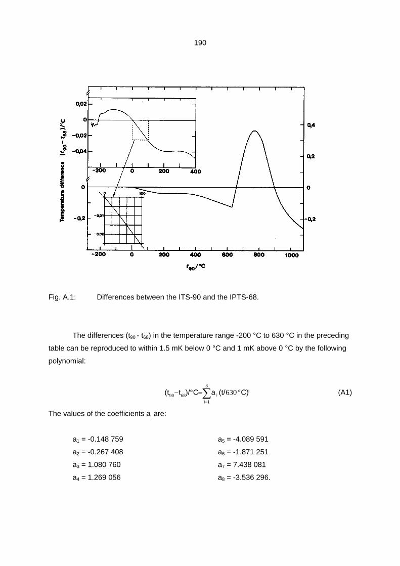
14. Page, 189, Appendix A: The values of (t90 – t68) in the range 630 °C to 1064 °C have been

revised [Rusby et al (1994)]. These revised values may be obtained from the following

equation:

∑=

°=°−5

906890 )/(/)(oi

ii CtbCtt

where b0 = 7.868 720 9 x 101

b1 = -4.713 599 1 x 10-1

b2 = 1.095 471 5 x 10-3

b3 = -1.235 788 4 x 10-6

b4 = 6.773 658 3 x 10-10

b5 = -1.445 808 1 x 10-13

15. Page 191, Appendix B: Two entries should be deleted: Amt für Standardisierung

Messwesen und Warenprüfung and Kamerlingh Onnes Laboratorium. Four other entries should be changed, as follows:

National Institute of Standards and Technology Process Measurements Division Chemical Science and Technology Laboratory Gaithersburg, Maryland 20899 U.S.A.

VI

Centre for Quantum Metrology National Physical Laboratory Teddington, TW11 OLW U.K. Fax: +44 181 943 6755

Institute for National Measurement Standards National Research Council of Canada Ottawa, Canada, K1A OR6

Nederlands Meetinstituut P.O. Box 654 2600 AR Delft (NL) Schoemakerstraat 97 2628 VK Delft (NL) Fax: +31 15 261 2971

16. Page 194, Appendix C: There are four (known) changes of address:

Scientific Instruments 4400 W. Tiffany Drive Mangonia Park West Palm Beach, Florida 33407 U.S.A. Fax: 1 (516) 881-8556

Cryogenic Ltd. Unit 30, Acton Park Estate London W3 7QE U.K. Fax: +44 181 749 5315

H. Tinsley and Co. Ltd. 275 King Henry's Drive Croydon CRO OAE U.K. Fax: +44 1689 800 405

Oxford Instruments Inc. Scientific Research Division Old Station Way Eynsham Witney Oxford OX8 1TL U.K. Fax: +44 1865 881 567

vii

Additionally, the Fax numbers for the first two firms listed are:

Cryo Cal Fax: 1 (612) 646-8718

Lake Shore Fax: 1 (614) 891-1392

17. Page 200, Appendix F: The original Appendix F should be deleted and replaced by

the following new Appendix F.

Appendix F

Interpolation Polynomials for Standard Thermocouple Reference Tables

i) All tables are for a reference temperature of 0 °C. ii) Throughout, E is in mV and t90 is in °C. iii) All of the polynomials (except one for Type K as noted below) are of the form

∑=

=n

i

ii tdE

090 )( . The values of n and of the coefficients di are listed for each thermocouple

type and each range.

1. Type T

a) temperature range from –270 °C to 0 °C: n = 14

d0 = 0.0 d7 = 3.607 115 420 5 x 10-13

d1 = 3.874 810 636 4 x 10-2 d8 = 3.849 393 988 3 x 10-15

d2 = 4.419 443 434 7 x 10-5 d9 = 2.821 352 192 5 x 10-17

d3 = 1.184 432 310 5 x 10-7 d10 = 1.425 159 477 9 x 10-19

d4 = 2.003 297 355 4 x 10-8 d11 = 4.876 866 228 6 x 10-22

d5 = 9.013 801 955 9 x 10-10 d12 = 1.079 553 927 0 x 10-24

d6 = 2.265 115 659 3 x 10-11 d13 = 1.394 502 706 2 x 10-27

d14 = 7.979 515 392 7 x 10-31

b) temperature range from 0 °C to 400 °C: n = 8

d0 = 0.0 d4 = -2.188 225 684 6 x 10-9

d1 = 3.874 810 636 4 x 10-2 d5 = 1.099 688 092 8 x 10-11

d2 = 3.329 222 788 0 x 10-5 d6 = -3.081 575 877 2 x 10-14

d3 = 2.061 824 340 4 x 10-7 d7 = 4.547 913 529 0 x 10-17

d8 = -2.751 290 167 3 x 10-20

viii

2. Type J

a) temperature range from -210 °C to 760 °C: n = 8

d0 = 0.0 d4 = 1.322 819 529 5 x 10-10

d1 = 5.038 118 781 5 x 10-2 d5 = -1.705 295 833 7 x 10-13

d2 = 3.047 583 693 0 x 10-5 d6 = 2.094 809 069 7 x 10-16

d3 = -8.568 106 572 0 x 10-8 d7 = -1.253 839 533 6 x 10-19

d8 = 1.563 172 569 7 x 10-23


d0 = 2.964 562 568 1 x 102 d3 = -3.184 768 670 10 x 10-6

d1 = -1.497 612 778 6... d4 = 1.572 081 900 4 x 10-9

d2 = 3.178 710 392 4 x 10-3 d5 = -3.069 136 905 6 x 10-13

3. Type E


d0 = 0.0 d7 = -1.028 760 553 4 x 10-13

d1 = 5.866 550 870 8 x 10-2 d8 = -8.037 012 362 1 x 10-16

d2 = 4.541 097 712 4 x 10-5 d9 = -4.397 949 739 1 x 10-18

d3 = -7.799 804 868 6 x 10-7 d10 = -1.641 477 635 5 x 10-20

d4 = -2.580 016 084 3 x 10-8 d11 = -3.967 361 951 6 x 10-23

d5 = -5.945 258 305 7 x 10-10 d12 = -5.582 732 872 1 x 10-26

d6 = -9.321 405 866 7 x 10-12 d13 = -3.465 784 201 3 x 10-29


d0 = 0.0 d6 = -1.919 749 550 4 x 10-16

d1 = 5.866 550 871 0 x 10-2 d7 = -1.253 660 049 7 x 10-18

d2 = 4.503 227 558 2 x 10-5 d8 = 2.148 921 756 9 x 10-21

d3 = 2.890 840 721 2 x 10-8 d9 = -1.438 804 178 2 x 10-24

d4 = -3.305 689 665 2 x 10-10 d10 = 3.596 089 948 1 x 10-28

d5 = 6.502 440 327 0 x 10-13

ix

4. Type K


d0 = 0.0 d6 = -5.741 032 742 8 x 10-13

d1 = 3.945 012 802 5 x 10-2 d7 = -3.108 887 289 4 x 10-15

d2 = 2.362 237 359 8 x 10-5 d8 = -1.045 160 936 5 x 10-17

d3 = -3.285 890 678 4 x 10-7 d9 = -1.988 926 687 8 x 10-20

d4 = -4.990 482 877 7 x 10-9 d10 = -1.632 269 748 6 x 10-23

d5 = -6.750 905 917 3 x 10-11

b) temperature range from 0 °C to 1372 °C:

The polynominal has the form

( )[ ]2901090

9

0

9686.126exp)( −+=∑=

tbbtdE i

ii

d0 = -1.760 041 368 6 x 10-2 d5 = -5.607 284 488 9 x 10-13

d1 = 3.892 120 497 5 x 10-2 d6 = 5.607 505 905 9 x 10-16

d2 = 1.855 877 003 2 x 10-5 d7 = -3.202 072 000 3 x 10-19

d3 = -9.945 759 287 4 x 10-8 d8 = 9.715 114 715 2 x 10-23

d4 = 3.184 094 571 9 x 10-10 d9 = -1.210 472 127 5 x 10-26

b0 = 1.185 976 x 10-1

b1 = -1.183 432 x 10-4

5. Type S

a) temperature range from -50 °C to 1064.18 °C: n = 8

d0 = 0.0 d4 = 3.220 288 230 36 x 10-11

d1 = 5.403 133 086 31 x 10-3 d5 = -3.314 651 963 89 x 10-14

d2 = 1.259 342 897 40 x 10-5 d6 = 2.557 442 517 86 x 10-17

d3 = -2.324 779 686 89 x 10-8 d7 = -1.250 688 713 93 x 10-20

d8 = 2.714 431 761 45 x 10-24

b) temperature range from 1064.18 °C to 1664.5 °C: n = 4

d0 = 1.329 004 440 85... d3 = -1.648 562 592 09 x 10-9

d1 = 3.345 093 113 44 x 10-3 d4 = 1.299 896 051 74 x 10-14

d2 = 6.548 051 928 18 x 10-6

x

c) temperature range from 1664.5 °c to 1768.1 °C: n = 4

d0 = 1.466 282 326 36 x 102 d3 = -3.304 390 469 87 x 10-8

d1 = -2.584 305 167 52 x 10-1 d4 = -9.432 236 906 12 x 10-15

d2 = 1.636 935 746 41 x 10-4

6. Type B

a) temperature range from 0° C to 630.615 °C: n=6

d0 = 0.0 d4 = 1.566 829 190 1 x 10-12

d1 = -2.465 081 834 6 x 10-4 d5 = -1.694 452 924 0 x 10-15

d2 = 5.904 042 117 1 x 10-6 d6 = 6.299 0347 09 4 x 10-19

d3 = -1.325 793 163 6 x 10-9

b) temperature range from 630.615 °C to 1820 °C: n = 8

d0 = -3.893 816 862 1 ... d4 = -1.683 534 486 4 x 10-10

d1 = 2.857 174 747 0 x 10-2 d5 = 1.110 979 401 3 x 10-13

d2 = -8.488 510 478 5 x 10-5 d6 = -4.451 543 103 3 x 10-17

d3 = 1.578 528 016 4 x 10-7 d7 = 9.897 564 082 1 x 10-21

d8 = -9.379 133 028 9 x 10-25

7. Type N

a) temperature range from -270°C to 0 °C: n = 8

d0 = 0.0 d4 = -4.641 203 975 9 x 10-11

d1 = 2.615 910 596 2 x 10-2 d5 = -2.630 335 771 6 x 10-12

d2 = 1.095 748 422 8 x 10-5 d6 = -2.265 343 800 3 x 10-14

d3 = -9.384 111 155 4 x 10-8 d7 = -7.608 930 079 1 x 10-17

d8 = -9.341 966 783 5 x 10-20


d0 = 0.0 d6 = -1.006 347 151 9 x 10-15

d1 = 2.592 939 460 1 x 10-2 d7 = 9.974 533 899 2 x 10-19

d2 = 1.571 014 188 0 x 10-5 d8 = -6.086 324 560 7 x 10-22

d3 = 4.382 562 723 7 x 10-8 d9 = 2.084 922 933 9 x 10-25

d4 = -2.526 116 979 4 x 10-10 d10 = -3.068 219 615 1 x 10-29

d5 = 6.431 181 933 9 x 10-13

xi

8. Type R

a) temperature range from -50 °C to 1064.18 °C: n = 9

d0 = 0.0 d5 = -4.623 476 662 98 x 10-14

d1 = 5.289 617 297 65 x 10-3 d6 = 5.007 774 410 34 x 10-17

d2 = 1.391 665 897 82 x 10-5 d7 = -3.731 058 861 91 x 10-20

d3 = -2.388 556 930 17 x 10-8 d8 = 1.577 164 823 67 x 10-23

d4 = 3.569 160 010 63 x 10-11 d9 = -2.810 386 252 51 x 10-27

b) temperature range from 1064.18 °C to 1664.5 °C: n = 5

d0 = 2.951 579 253 16... d3 = -7.640 859 475 76 x 10-9

d1 = -2.520 612 513 32 x 10-3 d4 = 2.053 052 910 24 x 10-12

d2 = 1.595 645 018 65 x 10-5 d5 = -2.933 596 681 73 x 10-16

c) temperature range from 1664.5 °C to 1768.1 °C: n = 4

d0 = 1.522 321 182 09 x 102 d3 = -3.458 957 064 53 x 10-8

d1 = -2.688 198 885 45 x 10-1 d4 = -9.346 339 710 46 x 10-15

d2 = 1.712 802 804 71 x 10-4

xii

xiii

Foreword

This monograph, published by the Bureau International des Poids et Mesures

(BIPM), has been compiled by the Comité Consultatif de Thermométrie, one of the

eight consultative committees established by the Comité International des Poids et

Mesures.

The approximations to the International Temperature Scale of 1990 described

here provide levels of accuracy that are adequate for the great majority of

thermometric requirements, and in general do so with greater convenience or at lower

cost than would be the case in realizing the ITS-90 itself. Thermometrists who do

require the accuracy only available from, or the imprimatur of, the ITS-90 are referred

to the text of that scale and, more particularly, to the companion monograph to this

one: "Supplementary Information for the ITS-90", also published by the BIPM in 1990.

The Comité Consultatif de Thermométrie expects to update both monographs

periodically, probably at intervals of the order of five to eight years.

H. PRESTON- THOMAS T.J. QUINN

President, CCT Director, BIPM

July 1990

xiv

Acknowledgments

This monograph has been prepared by the Working Group of the Comité

Consultatif de Thermométrie (CCT) identified hereunder. Although a large part of the

material originated with members of this Working Group, much also was originally

contributed by colleagues, either in our laboratories, or in other National Standards

Laboratories. In addition, (parts of) various drafts underwent critical review by some

members of the CCT and thermometry groups. We thank all of these people for their

assistance, and express special appreciation to H. Ronsin (Institut National de

Métrologie, France), B. Fellmuth (Amt für Standardisierung Messwesen und

Warenprüfung, German Democratic Republic), L. Crovini (Istituto di Metrologia "G.

Colonnetti", Italy), R.P. Hudson (then of Bureau International des Poids et Mesures,

Paris), R. Rusby (National Physical Laboratory, United Kingdom), and members of the

Temperature and Pressure Section (National Bureau of Standards, United States of

America). We also thank Mrs. P. Vineham (National Research Council of Canada) for

having typed so excellently and so patiently the several successive drafts of this

monograph.

Working Group 2: R.E. Bedford, National Research Council of Canada

Chairman

G. Bonnier, Institut National de Métrologie, France

H. Maas, Amt für Standardisierung Messwessen und

Warenprüfung, German Democratic Republic

F. Pavese, Istituto di Metrologia “G. Colonnetti”, Italy.

xv


Contents

1. Introduction 1

PART 1: TECHNIQUES AND THERMOMETERS FOR APPROXIMATING THE INTERNATIONAL TEMPERATURE SCALE OF 1990 9

2. Uniform-Temperature Enclosures 10

2.1 1 K to 300 K 10

2.2 150 K to 350 °C 14

2.3 300 °C to 1100 °C 16

3. Specialized Fixed Points 20

3.1 Fixed Points Below 0 °C 20

3.1.1 Superconductive Fixed Points 20

3.1.1.1 General Remarks 20

3.1.1.2 Requirements for Superconductive Fixed Points 21

3.1.1.3 Realization of Superconductive Fixed Points 22

3.1.2 Standard Reference Materials 22

3.1.3 Vapour Pressure Thermometers 24

3.1.4 Sealed Cells 25

3.2 Fixed Points -50 °C to 630 °C 28

3.2.1 Ice Point (0 °C) 28

3.2.1.1 Preparation of the Ice Point 32

3.2.1.2 Operating Conditions 33

3.3 Fixed Points above 630 °C 34

3.3.1 Copper 28.1% Silver 71.9% Eutectic Alloy 35

xvi

3.3.2 Melting Points of Gold (1064 °C), Palladium (1555 °C), and

Platinum (1768 °C) by the Wire-Bridge Method 36

3.3.3 Miniature Fixed Points for Thermocouple Calibrations 37

3.4 Fixed Points for Pyrometry 39

3.4.1 Blackbody Furnaces 39

3.4.2 Radiance Temperatures on Melting 41

4. Germanium Resistance Thermometers 42

4.1 Principles and Range of Use 42

4.2 Fabrication 42

4.3 Electrical Characteristics 45

4.3.1 Method of Measurement 45

4.3.2 Resistance/Temperature Characteristics and Sensitivity 46

4.3.3 Stability 48

4.3.4 External Influences 49

4.4 Thermal Properties 49

4.4.1 Self-heating and Thermal Anchoring 49

4.4.2 Time Constant 52

4.5 Calibration and Interpolation Formulae 52

5. Rhodium-lron Resistance Thermometers 55

5.1 Range of Use and Sensitivity 55

5.2 Fabrication 55

5.3 Reproducibility and Stability 57

5.4 Self-heating 58

5.5 Calibration and Interpolation 58

6. Vapour Pressure Thermometry 60

6.1 Two-Phase Equilibrium 62

6.2 Technical Details of Construction 67

6.2.1 Bulb 67

6.2.2 Connecting Tube 69

6.2.3 Pressure Sensor 69

6.2.4 Filling the Thermometer 71

6.3 Metrological Characteristics and Measurement Corrections 72

xvii

6.3.1 Extent of Sensitivity and Measurement 72

6.3.2 Reproducibility and Accuracy 72

6.3.3 Response Time 75

6.3.4 Correction for Aerostatic Pressure 75

6.3.5 Thermomolecular Effect 75

6.3.6 Corrections Due to Impurities 79

6.3.7 Particular Problems with Helium [Cataland et al. (1962), Kerrik (1970),

Montgomery and Pells (1963), Rusby and Swenson (1980)] 83

6.3.8 Other Corrections 84

6.4 Conclusion 84

7. Magnetic Thermometry 85

7.1 Magnetic Thermometer 85

7.2 Technical Aspects of Magnetic Thermometry 86

8. Platinum Resistance Thermometers 88

8.1 General Remarks 88

8.2 Interpolation Equations for Standard Platinum Resistance

Thermometers 89

9. Platinum Thermocouples 95


9.2 Construction 96

9.3 Annealing of the Thermoelements 98

9.4 Guidelines for Proper Handling and Use -Installation and Sources of

9.5 Errors 99

9.6 Approximations to the ITS-90 102

10. Infrared Radiation Thermometers 104

PART 2: TECHNIQUES AND THERMOMETERS TRACEABLE TO THE INTERNATIONAL TEMPERATURE SCALE OF 1990 107

11. Carbon Resistance Thermometers 108

11.1 Fabrication and Use 108

11.2 Resistance-Temperature Characteristics and Sensitivity 109

xviii

11.3 Thermal Contact 111

11.4 Response Time 111

11.5 Influence of External Factors 112

11.6 Stability and Reproducibility 113

11.7 Calibration and Interpolation Formulae 114

12. Carbon-Glass Resistance Thermometers 116

12.1 Fabrication 116

12.2 Resistance-Temperature Characteristics; Sensitivity; Calibration 116

12.3 Stability 117

13. Platinum-Cobalt Resistance Thermometers 119

14. Diode Thermometers 120

15. Liquid-in-Glass Thermometry 123

16. Industrial Platinum Resistance Thermometers 129

16.1 Quality of Industrial Platinum Resistance Thermometers 129

16.1.1 Stability 132

16.1.2 Self-heating 134

16.1.3 Response Time 137

16.2 Interpolation Equations for Industrial Platinum

Resistance Thermometers 137

16.3 National and International Specifications for IPRTs 139

17. Thermistors 145

18. Base-Metal Thermocouples 147


18.2 Types of Base-Metal Thermocouples 147

18.2.1 Type T Thermocouple 148

18.2.2 Type J Thermocouple 148

18.2.3 Type K Thermocouple 148

18.2.4 Type E Thermocouple 149

18.2.5 Type N Thermocouple 149

18.2.6 Tungsten-Rhenium Thermocouple 149

18.3 Construction 150

18.3.1 Thermoelements 150

xix

18.3.2 Sheaths 150

18.3.3 Protection Tubes 152

18.3.4 Thermocouple Construction 152

18.3.5 Circuit Construction 153

18.4 Annealing of the Thermoelements 155

18.5 Guidelines for Proper Handling and Use -Installation and

Sources of Errors 156

18.6 Calibration of Base-Metal Thermocouples 158

19. Thermometry in Magnetic Fields 160

20. References 169

Appendices

A. Differences between the ITS-90 and the EPT -76, and between the

ITS-90 and the IPTS-68 189

B. Addresses of National Standards Laboratories 191

C. Some Suppliers of Various Cryogenic Thermometers 194

D. Calculations Relative to the Filling of a Vapour Pressure Thermometer 196

E. Calculation of the Aerostatic Pressure Correction for a Vapour

Pressure Thermometer 199

F. Interpolation polynomials for Standard Thermocouple Reference Tables 200

1

1. Introduction

The Comité Consultatif de Thermométrie (CCT) has always had as its chief concern

the perfecting of the International Temperature Scale (ITS) and, consequently, has been

occupied with thermometric measurements of the very highest accuracy. There are many

laboratories in the world, including even some of the national standardizing laboratories in

countries adhering to the Convention du Metre, that, while requiring temperature

measurements to be related to the ITS, do not require this ultimate accuracy. In an attempt

to address this need, the CCT assigned to a Working Group the task of preparing a

monograph describing methods for approximating the ITS that are simpler and more

practicable than the fundamental definition, giving estimated accuracies of the various

approximations. That the need for this information is high can be inferred from the result of

a study in the U.S.A. [Frost and Sullivan (1984)] which reveals that temperature is the most

commonly measured physical variable today. The study forecast annual expenditures in

the U.S.A. of $0.9 x 109 on temperature measurement and control devices and

instrumentation by 1988 for a real annual growth rate of 10% in the industrial temperature

instrumentation market over a 5-year span. This monograph is meant to be a companion to

"Supplementary Information for the ITS-90" [CCT (1990)], a forthcoming revision of

"Supplementary Information for the IPTS-68 and the EPT- 76" [CCT (1983)]. The latter is

directed to those who wish to realize the ITS-90 with accuracies ranging from moderately

high to the very highest level; the present monograph is to give guidance to those who wish

to approximate the ITS-90 using simpler techniques and for whom those levels of accuracy

are unnecessarily high. It is clear that in such a monograph care must be taken to

emphasize that the approximations described do not constitute official recipes for realizing

the ITS-90, different from but less accurate than the fundamental definition. Such a

proliferation of "official" scales would be highly undesirable.

This monograph therefore provides information on how one can approximate the ITS-

90 to a modest but specified level of accuracy with a variety of techniques. It necessarily

includes considerable discussion of the sensors themselves - their properties, reliability and

limitations, and guidelines for proper handling and use - but this discussion is in no way

exhaustive. A large literature already exists on these sensors to which the reader is referred

for extensive treatments.

2

For a formal realization of the ITS-90, the response of (one of) the defining

instruments* is measured at the appropriate defining fixed points and the thermometer is

then used to interpolate temperatures between the fixed points according to the

relationships specified in the definition of the scale. Methods for doing this have been

outlined [CCT (1990)]. For the approximations described herein the thermometer has to be

calibrated in a way that can be related to such a formal realization of the ITS-90. This can be

done either by a comparison calibration or by using fixed points, approaches which differ

slightly but subtly. Formerly, comparison calibrations were the most-used mechanism for

dissemination of the ITS, but more and more the fixed-point method is being used. In France

and in the German Democratic Republic, for example, the ITS-90 is already disseminated

largely in terms of calibrated fixed point devices.

A comparison calibration (or simply a calibration) of a thermometer usually implies a

direct comparison of the thermometer response with that of a calibrated defining instrument

at many temperatures in some sort of isothermal environment (such as a liquid bath or a

metal block in an electric furnace). Either the calibration itself, or, more usually, the

calibration of the defining instrument, is carried out in a national standards laboratory or in

an accredited secondary laboratory, thereby ensuring a direct link to the ITS-90. For a great

many users this can be the simplest and most straightforward way to obtain direct access to

the ITS-90. It can be, but is not necessarily, inexpensive. Temperatures are measured

directly on the ITS-90 if the calibrated thermometer is one of the defining instruments. Under

the best conditions the uncertainties in measured temperatures can be as small as those of

the calibration, which in turn may be within a factor of two or three of the standards

laboratory's primary realization. More generally, of course, the accuracy will be determined

by the quality of the thermometer and by the measurement procedures. One disadvantage

of direct calibration by a standards laboratory is that it does not constitute an independent

realization of the ITS-90, if such is required. Another is that any calibration by comparison

involves the transport of thermometers between laboratories, a procedure that can affect

their reliability.

There are many national standards laboratories world-wide that offer a calibration

service over the complete range of the ITS-90 (see Appendix A, which is not necessarily

complete). Some standards laboratories are not prepared to calibrate large numbers of

_________________________________________________________________________

* The term "defining instrument" is used to mean any one of the standard thermometers

specified in the text of the ITS-90 for interpolating between defining fixed points.

3

thermometers except in special extenuating circumstances; these laboratories are

prepared, however, to calibrate thermometers intended to be supplied to national

secondary calibration services.

Commonly, a user of large numbers of thermometers (university, factory, etc.) will not

rely upon a national standards laboratory for all of its calibrations, but instead will acquire a

selected number of calibrated thermometers as its secondary standards against which it

will calibrate its working thermometers (or, if the user is itself another standards laboratory

or an accredited calibration laboratory, its customers' thermometers). In such

circumstances it is highly desirable to maintain a minimum of three secondary standards of

each type that have undergone reasonably recent primary calibrations. One or, usually, two

of these will become general working standards; at least one, and preferably two or more,

will see very little service except for periodic checks of the calibrations of the working

standards and of each other. In this way, any apparent changes in calibration can easily be

traced to the offending instrument. The more secondary standards that are available, the

more reliable this procedure becomes. The thermometers used as secondary standards

will almost always be standard platinum resistance thermometers (SPRTs) ; germanium or

rhodium-iron resistance thermometers; platinum 10% rhodium/platinum, platinum 13%

rhodium/platinum, gold/platinum, or palladium/platinum thermocouples; tungsten strip-

filament lamps; or infrared radiation thermometers, depending upon the temperature range

required and the instrument to be calibrated. These standards should be maintained

according to the procedures outlined in the "Supplementary Information for the ITS-90"

[CCT (1990)]. It is recommended that fixed points (for example, triple points of water,

gallium, or cryogenic substances) also be obtained so as to monitor the stability of

resistance thermometers. For SPRTs this serves two important additional purposes: (a)

changes in the resistance (R(t)) of an SPRT due to cold work, oxidation, strain, etc. are, to

a first approximation, proportional to R(t) so that the resistance ratio W(t) = R(t)/R(0.01 °C)

remains relatively unchanged. The ability to monitor a particular value of R(t), such as R(t)

at a fixed point, then leads to higher temperature measurement accuracy. (b) W(t) is

independent of the unit used to measure R(t) so long as all resistance values are

measured with the same instrument (for example, bridge and standard resistor). Thus,

laboratory measurement of resistance at a fixed point as opposed to reliance on a

calibration-supplied value of resistance at that fixed point obviates the need for

measurement in ohms.

4

The tungsten strip-filament lamp mentioned in the preceding paragraph is not itself a

thermometer, but acts as a transfer device. The lamp is calibrated with a standard optical

pyrometer in terms of spectral radiance temperature at a particular wavelength versus

current, and this calibration is subsequently transferred to another pyrometer.

For a calibration using fixed points (which has been called a secondary realization,

but this term is not recommended), the thermometer is calibrated at a number of such

points (that may include both defining and secondary fixed points) and temperatures are

interpolated between fixed points according to a functional (usually an empirical)

relationship that experience has shown will generate values of temperature on the ITS-90 to

within some specified degree of accuracy. Secondary fixed points are fixed points that are

not used in the definition of the ITS-90, but which have been well-characterized, and the

temperatures of which have been carefully determined on the ITS-90. Bedford et al. (1984)

give recommended values of temperatures, together with an assessment of their

uncertainties, for a large number of secondary fixed points. The values of temperature,

which are on the IPTS-68, can be converted to the ITS-90 using the tables included here in

Appendix A.

A thermometric reference material might, in some circumstances, also be used in

the sense of a secondary fixed point. Caution should be exercised, however, in the use of

thermometric reference materials, which differ in principle from fixed points. A fixed point

(whether primary or secondary) is a phase transition temperature of a substance of

extremely high purity; any two samples of the substance will exhibit precisely the same

transition temperature, so long as the experimental apparatus (furnace, cryostat) is properly

designed and the thermometer is in temperature equilibrium with the sample. A

thermometric reference material, on the other hand, is simply a batch of certified material

from which samples can be drawn; a sample of this material, when used according to a

specific recipe, undergoes a phase transition at a temperature that has been previously

measured and certified with a calibrated thermometer. The material need not be especially

pure, and the assigned transition temperature applies only to the particular lot from which

the sample is drawn. Another lot of nominally the same substance may have a different

transition temperature. In this monograph the many references to secondary fixed points

should not be construed as being applicable to reference materials. A thermometric sealed

cell, depending upon its construction, can be used either in the sense of a fixed point or of a

reference material [Pavese (1980), (1986)]. If a reference material is used as a fixed point,

the value of temperature associated with it should be that given by the supplier.

5

The accuracies with which temperatures may be referred to the ITS-90 as a result of

a comparison calibration or a calibration with fixed points are comparable; if anything, the

former is the more accurate except near the fixed point temperatures unless many fixed

points are used. It is difficult to make any single statement regarding the limits of accuracy

that may apply. As a rough guide, the largest uncertainty for any technique described herein

will be ± 0.05 K below 100 K, ± 0.2 K near and above room temperature, ± 0.5 K up to 1000

°C, and ± 1 to 2 K above. Many of the techniques, of course, may give substantially better

results than this. In Table 1.1 are listed all of the thermometers discussed in this

monograph, their temperature ranges under various conditions, and typical associated

uncertainties.

The ITS-90 became the officially-recognized International Temperature Scale on

January 1, 1990. In this monograph there are a few unavoidable references to its

predecessor, the IPTS-68. Furthermore, there are undoubtedly users of this monograph who

are measuring temperatures with thermometers calibrated on the IPTS-68. We emphasize

that any temperature T68 (or t68) can be converted to its equivalent value of T90 (or t90) by use

of the tables given here in Appendix A. Similarly, any previous edition of the ITS can be

used to approximate the ITS-90 to within the combined accuracies of the associated

conversion tables.

This monograph is divided into two parts. Part 1 includes those methods and

thermometers that are considered to be best suited for directly approximating the ITS-90,

and the associated calibration techniques. Part 2 deals with a number of thermometers that

are important because they are widely used or are used for special purposes, but that are in

general less accurate than those of Part 1, and for which temperatures measured with them

must still be traced to the ITS-90. Thus, for example, approximations based upon SPRTs

are described in Part 1 but treatment of industrial platinum resistance thermometers (IPRTs)

is relegated to Part 2 because, although IPRTs are in wide use, they are as a class not

accurate enough for approximating the ITS-90 directly in the sense defined here.

International specifications for IPRTs and standard thermocouple reference tables as

developed for use with the IPTS-68 are included herein. At the time of writing,

corresponding specifications and tables with respect to the ITS-90 had not yet been

published. Approximate equivalents can be obtained using the tables in Appendix A.

There is, naturally, a degree of overlap between the material contained herein and

that in "Supplementary Information for the ITS-90" [CCT (1990)]. Methods for highly

accurate fixed point realizations, for example, are described in some detail there, so will

6

not be repeated here, but several special ways to use fixed points for approximating the

ITS-90 are described in Chapter 3. On the other hand, there is some duplication in

descriptions of the various sensors since all of the defining instruments are also used for

secondary measurements. Except for the standard platinum resistance thermometer, there

is a rather fuller description of the sensors in the present monograph. For the platinum 10%

rhodium/platinum thermocouple*, in particular, which is one of the most important

thermometers for approximating the ITS-90 even though it is no longer a defining instrument

of the ITS, the information contained in Chapter 5 of the "Supplementary Information for the

IPTS-68 and the EPT-76" [CCT-1983] has been included and substantially augmented here,

and has been deleted from the revised "Supplementary Information for the ITS-90" [CCT

(1990)].

_________________________________________________________________________

* In this monograph, specific thermocouple designations are written with the positive

element first, separated from the negative element by the oblique symbol. Frequently,

also, they will be written in an abbreviated form: platinum 10% rhodium/platinum will

also be written as Pt10Rh/Pt, for example. Standard international letter designations,

such as Type S for Pt10Rh/Pt, are also used of course.

7

Table 1.1: Summary of Some Properties of Most-Commonly-Used Thermometers

Usual Thermometric Typical Thermometer Temperature Quantity Uncertainty

Range

Germanium 1 K to 100 K elec. resist.* ∆T / T < 2x10-4

Rhodium-lron 0.5 K to 30 K elec. resist.* 0.3 mK

Platinum-Cobalt 2 K to 20 K elec. resist.* 10 mK

(industrial type)

Carbon 0.5 K to 30 K elec. resist.* ∆T / T < 5x10-3

Carbon-glass 0.5 K to 100 K elec. resist.* ∆T / T < 1 x1 0-3

Diode 4 K to 300 K junction voltage -50 mK

Vapour-pressure various subranges pressure -1 mK between 0.5 K and 100 K

Mercury-in-glass -50 °C to 250 °C thermal expansion 0.1 K of mercury

Thermocouples 4 K to 2500 °C thermoelectromotive force

Type S -50 °C to 1600 °C 0.3 K < 1000 °C 1 K > 1000 °C

Type R -50 °C to 1600 °C 0.3 K < 1000°C 1 K > 1000 °C

Type B 300 °C to 1800 °C 0.5 K to 2 K

Type T -200 °C to 350 °C 0.1 K

Type E -200 °C to 870 °C 0.1 K < 300 K 1 K > 300 K

Type J 0 °C to 760 °C 0.5 K < 300 °C 2 K > 300 °C

Type K -200 °C to 1260 °C 0.1 K < 200 °C 1 K 200-1000 °C

3 K > 1000 °C

Type N 0 °C to 1300 °C 0.1 K < 200 °C 0.5 K 200-1000 °C

3 K > 1000 °C

W/Re 1000 °C to 2400 °C 3-10 K

_________________________________________________________________________

* elec. resist. is the electrical resistance

8

Table 1.1: (Continued)

Usual Thermometric Typical Thermometer Temperature Quantity Uncertainty Range

Thermistor -80 °C to elec. resist.* 0.1 K (much better 250 °C if use confined to very small temperature range)

Platinum: SPRT 14 K to 630 °C elec. resist.* 0.5 mK IPRT 20 K to 600 °C 50 mK

Radiation 100 °C to 3000 °C spectral radiance 1 K < 1000 °C of source 5 K > 1000 °C

_________________________________________________________________________

* elec. resist. is the electrical resistance

9

PART 1: TECHNIQUES AND THERMOMETERS FOR APPROXIMATING THE INTERNATIONAL TEMPERATURE SCALE OF 1990

The most common and best-characterized thermometers for very low temperature

use are those that relate temperature to electrical resistance. In Part 1 there is a discussion

of germanium, rhodium-iron, and platinum resistance thermometers together with their

associated calibrations and interpolation formulae for approximating the ITS-90. The use of

germanium is normally restricted to below 30 K. The same has been true for rhodium-iron

although the chief reason for not using it to near 300 K has been competition from platinum.

With platinum, calibration at a few fixed points coupled with simple interpolation will

reproduce the ITS-90 moderately accurately. Germanium and rhodium-iron thermometers,

on the other hand, must be individually calibrated because no two thermometers of the same

type have exactly similar resistance/temperature characteristics, and there must be

calibration at many points because interpolation of the resistance/temperature relationship is

difficult. They are used as transfer standards for maintaining the ITS-90 below about 25 K,

defined in terms of thermodynamic thermometry.

Germanium resistance thermometers are small, relatively inexpensive, and very

sensitive at the lower end of their range. Standard-type rhodium-iron resistance

thermometers are much larger, much more expensive and less sensitive than germanium,

but are more stable and have a wider range of use. Platinum costs the same as, or more

than, rhodium-iron, and is the clear choice above about 25 K. Both platinum and rhodium-

iron are extremely stable; with proper handling, which means treating the thermometers as

fragile and not subjecting them to mechanical shocks or vibrations, variations as large as a

millikelvin are unusual. Germanium thermometers are about an order of magnitude less

stable.

Vapour pressure thermometry and magnetic thermometry are also discussed in Part

1 because of their fundamental use. No comparable treatment of the former appears to exist.

Platinum thermocouples and infrared radiation thermometers are also included in Part 1

because they are widely used to approximate the ITS-90.

The discussion of these various thermometers is preceded by a description of the

methods, and hence of cryostats, baths, and furnaces, for attainment of uniform temperature

environments (Chapter 2) and by some discussion of fixed points (Chapter 3), the latter

intended to complement, rather than duplicate, that in "Supplementary Information for the

ITS-90" [CCT (1990)].

10

2. Uniform-Temperature Enclosures

Calibration of thermometers requires uniform-temperature enclosures. All of the

apparatuses described here to produce such enclosures may be constructed in the

laboratory, or, alternatively, may be obtained commercially. The latter tend to be more costly

and to provide poorer, although adequate, uniformity. For comparison calibrations, the

uncalibrated thermometer and the laboratory standard are mounted in such a way as to be in

good mutual thermal contact, as in a solid metal block or a stirred liquid. Significant errors

can be avoided by proper attention to immersion depths, heat transfer along thermometer

leads, thermal time lags, thermometer self-heating, temperature differences within the

enclosure, radiation exchange with the environment, and so on. The type of enclosure used

depends upon the temperature range involved.

2.1 1 K TO 300 K

Several apparatuses that serve for the calibration of thermometers have been

described. The temperature stability and uniformity of the apparatuses depend upon both

their thermal design and the quality of the associated temperature controller. One that is

simple, that has worked extremely well for calibrating capsule PRTs, and that can be used

with germanium (Ge) or rhodium-iron (RhFe) resistance thermometers is shown in Fig. 2.1.

A small copper block with holes for four thermometers is surrounded by two concentric

copper radiation shields in an insulated container which is open at the bottom. The container

hangs by a thin-walled metal tube in a liquid helium dewar. To prevent heat transfer along

the thermometer leads, the latter pass through insulated holes in the copper block and one

of the shields. Heaters are wound on both the block and the shields, and the temperature

difference between them is measured with differential thermocouples. The block is cooled to

liquid helium temperatures and the liquid is then blown out of the insulated container, leaving

helium gas at atmospheric pressure therein. The liquid helium remaining in the dewar

provides the necessary cooling. The block is heated to, and then maintained at, each

desired temperature in turn, the shield temperatures being adjusted to be that of the block by

a servo-control. The apparatus requires no vacuum feed-throughs for the leads and the

thermometers rapidly reach equilibrium as a result of the good thermal contact between the

block and the thermometer provided by the helium gas. With this system a PRT can be

calibrated to within 1 mK.

11

Fig. 2.1: One form of apparatus used at NRC for calibration of resistance thermometers from

4.2 K to 273.15 K: A, metal cover; B, copper shields; C, copper block; D, expanded

polystyrene; E, capsule PRT; F, liquid helium.

An alternative procedure that is also widely used is to place the thermometers in a

copper block that is enclosed within suitable radiation shields in an evacuated cryostat as

shown in Fig. 2.2 (see, for example, Rusby et al. (1972), Compton and Ward (1975), or

Besley and Kemp (1977)). Details of operation are given in the suggested references. It is

sometimes useful to design the cryostat in a modular way to allow for the use of a single

apparatus for different experiments. This may be facilitated by the incorporation of a

cylindrical re-entrant well in the tube connecting the cryostat chamber to the part of the

apparatus that is at room temperature. In this way, different modules, designed for different

experiments, can be interchanged from the top flange, without one's having to disassemble

the cryostat itself [see Pavese (1981 )].

For temperatures above 4 K, it is also possible to use closed-cycle refrigerators, so

avoiding conventional liquid refrigerants and allowing convenient and faster operation. The

thermal design of measuring modules for such a system is similar to that of a flow cryostat

(Fig. 2.3) [Blanke and Thomas (1979)], but care must be taken to prevent mechanical -

vibrations from adversely affecting the thermometer.

12

Fig. 2.2: Cryostat for calibration of resistance thermometers: D, outline of helium dewar; HE,

liquid helium reservoir; PT, pumping tube; SS, stainless-steel vacuum can; I,

indium seal; R, radiation shield; A, one of four access tubes for wires; B, binding

post for wires; T, one of four support tubes; V, vacuum; S, temperature control

sensor; H, heater; C 1, copper thermometer block; C2, copper isothermal shield; P,

platinum thermometer; G, germanium thermometer [after Rusby et al. (1972)].

13

Fig. 2.3: Flow cryostat, shown with a vapour pressure bulb fitted: 1, pressure tube with

radiation traps; 9, bulb with thermometers; 15, 24, vacuum space pumped through;

8, outer shield, nitrogen cooled through inlet 13 and coil 7; 20, inner shield, helium

cooled through syphon 14 and coils 12 and 21; 23, isothermal shield, with internal

independent vacuum 22; 16, thermometers : for temperature regulation of the shield.

[Blanke and Thomas (1979)].

The sealed-cell cryostat of Ancsin and Phillips (1984) can also be used as a

comparator over the temperature range 84 K to 400 °C (see Sec. 3.1.4).

In any of these systems, it is important that the thermometers be in good thermal

contact with the block, as through the use of a vacuum grease. It is also important to prevent

heat exchange between the thermometer and room temperature via the connecting leads;

for this reason the thermometer leads, and an appropriate length [Hust (1970); Fellmuth and

Seifert (1988)] of the connecting wires must be put in good thermal contact with the

measuring block or with a body maintained at block temperature. However, this

14

procedure must not prejudice the maintaining of a sufficiently high electrical insulation

resistance. The necessary resistance depends upon the accuracy required and the

thermometer resistance. In measuring the insulation resistance, care must be taken not to

damage the thermometer by too-high currents from the high-resistance-measuring device. In

general, the minimum allowable insulation resistance is tens of megohms. The wires coming

into the experimental chamber of the cryostat should also be thermally anchored at the

refrigerant temperature. A suitable thermal-anchoring material is made of copper evaporated

over a thin plastic foil such as Kapton.

2.2 150 K to 350 °C In this range the most convenient enclosures for mounted thermometers are stirred-

liquid baths. The approximate temperature ranges that may be covered by various liquids

are: 150 K to 225 K, isopentane; 225 K to 20 °C, methyl alcohol; 2 °C to 90 °C, water, with

the range extendable to -5 °C by the addition of a small quantity of glycol; 50 °C to 350 °C,

mineral or synthetic oils. The essential features of a bath used at NRC are shown in Fig. 2.4.

The liquid is contained between 50 cm long concentric cylinders of diameters about 10 cm

and 6 cm respectively. A propeller driven through a seal at the bottom of the bath and with

appropriate anti-spin vanes forces the liquid up the inner cylinder and down between the

two. An immersion heater between the cylinders controls the temperature and a second

heater on the outer cylinder maintains the external temperature a few degrees below the

required calibration temperature. For the water bath, cooling is obtained by circulating Freon

through the refrigerant coils shown on the outer shell. With the oil bath, which operates only

above ambient temperature, the refrigerant is unnecessary. For the alcohol or isopentane

baths, liquid nitrogen or solid carbon dioxide are the usual refrigerants. The thermometers to

be calibrated are mounted at suitable depths within the inner cylinder. Uniformity of

temperature to better than 10 mK, and with care to within 1 to 3 mK, within this inner cylinder

is readily achieved. Other variations of this general design are described by Quinn (1983)

and Pavese and Coggiola (1972).

With the oil baths, light mineral oils are used up to about 200 °C, and heavy oils up to

about 350 °C or even 375 °C on occasion. The upper limit is set by the flash point of the oil

or by the tendency of the oils to carbonize. The lower limit is that at which the viscosity has

become too high for efficient heat transfer to be maintained. In using an oil bath, it is

essential to provide a proper venting system to remove the noxious fumes from the

laboratory. It is also advisable to keep a suitable fire extinguisher at hand if the bath

15

Fig. 2.4: Stirred liquid bath for use from -5 °C to 350 °C: A, top cover, bakelite; B, insulation,

expanded polystyrene; C, bakelite; D, top ring, bakelite; E, weir height adjustment

screw; F, splash shield; G, weir, brass; H, water container, brass; J, overflow tube,

german silver; K, drain, german silver; L, insulation, mica; M, outer heater; N,

insulation, fiberglass; O, copper sheet; P, refrigeration coil; Q, insulation, fiberglass;

R, propeller, 4 blades brass; S, closure housing including seals and lubricants; T,

tube, german silver; U, o-ring seat; V, lower bearing, teflon; W, upper bearing,

teflon; X, anti-spin vane; Y, screen, copper.

temperature is to be raised to near the flash point because ignition may occasionally occur

below the expected flash point.

16

2.3 300 °C to 1100 °C For temperatures above the range of stirred oil, no completely satisfactory bath is

available. A salt bath (containing a mixture of equal parts of potassium nitrate and sodium

nitrite) will provide an extremely uniform temperature from about 250 °C to 550 °C, but has

substantial drawbacks. These include: a highly corrosive action on the bath container and on

any devices inserted into the salt (a quartz-sheathed thermometer must be protected from

the salt by an auxiliary Pyrex protection tube); a salt residue left on a device after calibration

which is often difficult to remove; a potentially dangerous condition during heat-up if

expansion of liquid is prevented by entrapment in solid salt; an extremely long heat-up time

for the solid phase; possible violent splatter when foreign (organic) materials come in contact

with the salt; requirement for venting fumes; and a generally messy housekeeping problem.

Industrial safety codes for the operation of salt baths should be consulted [for example,

HMSO (1964)].

An alternative to the salt bath is a fluidized bed, or fluidized powder bath. This can be

capable of operation over an extremely wide range (from below ambient to 1100 °C) but it is

difficult to obtain within the working volume a temperature that is uniform enough. The

fluidizing medium is usually very finely powdered aluminium oxide through which dry air,

nitrogen, or argon is allowed to flow slowly upward from an underlying porous diffuser of

metal or ceramic. When fluidization begins, the individual AI2O3 particles circulate freely, and

the powder takes on many of the properties of a liquid. The appearance is much like that of

swirling cream with gentle surface bubbling. The powder tends to rise and migrate slowly

from the centre to the walls. Heat is supplied in much the same way as in a liquid bath.

Frequently, in the higher temperature units, a layer of zirconium oxide that does not fluidize

but assists in the diffusion and inhibits the burning of the porous plate lies between the AI2O3

and the solid diffuser plates. Typical temperature differences in the fluidized bath range from

tenths of kelvins to as high as a few kelvins. If a metal block is used within the fluidizing

medium, better uniformity is possible. In addition to a frequently inadequate temperature

uniformity, another disadvantage is the deposition of AI2O3 dust on everything near the bath.

Care must be taken to avoid mechanical vibrations arising from the circulation of the fluid

powders.

Wire-wound resistively-heated electric furnaces are the most common uniform-

temperature enclosure above the range of liquid baths. These are essentially the same as

those described in "Supplementary Information for the ITS-90" [CCT (1990)] for the

realization of metal freezing points. A metal block (aluminium, copper, Inconel) is

17

contained within a cylindrical ceramic muffle on which the heaters are wound. The main

heater runs the whole length of the muffle, while smaller ones are placed either over it or

within the muffle near each end, compensating for heat losses and thereby lengthening the

uniform-temperature zone. The whole is suitably insulated. With care, for a 60 to 90 cm

furnace, it is possible to adjust the heater powers so as to obtain a central 20 to 30 cm zone

that is uniform in temperature to some tenths of a kelvin. The convenient upper temperature

limit for such furnaces is 1100 °C, up to which Nichrome or Kanthal heater windings have

long lifetimes. For higher temperatures one must resort either to expensive platinum-alloy

heaters or to refractory-metal heaters that require protection from air or oxygen.

A simpler arrangement with even better temperature uniformity uses a cylindrical

heat-pipe liner within the furnace muffle. In this case a single heater will suffice. A heat pipe

is essentially a closed tube or chamber whose inner surfaces are lined with a porous-

capillary wick. The wick is saturated with the liquid phase of a working fluid and the

remaining volume of the tube contains the vapour phase. Applied heat vaporizes the working

fluid in some sections, resulting in a pressure difference that drives vapour to cooler regions

where it will condense, releasing the heat of vaporization in that section of the pipe.

Depletion of liquid by evaporation causes the liquid-vapour interface to enter into the wick

surface. The capillary pressure developed there pumps the condensed liquid back for re-

evaporation. That is, the heat pipe can continuously transport the heat of vaporization from

the evaporator to the condenser section.

The amount of heat that can be transported in this way is several orders of

magnitude larger than that which can be transported in a conventional system; the heat pipe

acts as a tube of extremely high thermal conductivity. Hence, when it is placed within an

already-heated furnace it increases the uniformity immensely. Quinn (1983) gives a useful,

more detailed discussion. The working fluid is usually sodium or potassium for heat pipes of

interest here. A metal block may be placed within the heat pipe, but in many cases may be

unnecessary. Care must be taken in the use of metal-enclosed sodium or potassium in heat

pipes; the usual precautions for use of these metals should be taken.

A more sophisticated use of the heat pipe is in the pressure-controlled or gas-

controlled heat pipe [see, for example, Bassani et al. (1980)]. The cylindrical heat pipe is

installed in a conventional electric furnace as above, but in this case most of the applied heat

is concentrated near one end (the concentrator); a vertical (or tilted, for vertical furnace

operation) water-cooled chimney (the condenser) is attached at the other

18

end; and an inert buffer gas (helium) is maintained over the working fluid (sodium) vapour,

the buffer-gas pressure being externally controlled by conventional techniques. The furnace

temperature can be changed from one level to another by changing the buffer-gas pressure;

re-equilibration at the new level is rapid, typically within a few tenths of a kelvin in 20 minutes

for a 50 K change. A standard pressure and temperature feedback control system allows the

temperature to be controlled at a given level to within a few mK. The response to small

pressure changes is very rapid, the speed being determined more by the temperature-

sensor response than the heat-pipe response. Temperature uniformity within the furnace to

within a few mK is possible. With sodium as the working fluid, the heat-pipe furnace is

operable from about 550 °C to 1100 °C; with potassium, from about 400 °C to 950 °C.

Another type of furnace used for the calibration of thermocouples is the electric tube

furnace, shown schematically in Fig. 2.5 [Dauphinee (1955)]. The cylindrical Nichrome

furnace tube about 3 cm in diameter and 50 cm long forms part of a one-turn secondary of a

high-power transformer, and is resistively heated by the high ac secondary current. A silica

tube is placed inside the furnace tube, and the thermocouples to be calibrated are inserted

inside this with their tips welded or otherwise physically joined together. The furnace is

uninsulated so its temperature can be changed very rapidly. A typical calibration run with

Pt10Rh/Pt thermocouples takes 2 hours from ambient to 1100 °C and down again. This high

speed is possible because the absolute emfs of the unknown and the standard need not be

simultaneously known, but only the slowly-changing difference between them. Typically, with

Pt10Rh/Pt calibrations for example, this difference when the furnace is heating will have

slightly different values from when it is cooling, but it can be shown that the mean of the two

is the same as the steady-state difference. With (even slightly) dissimilar base-metal

thermocouples, the furnace temperature must be stabilized at the desired calibration points

before the emfs are measured. In this furnace there is really no constant temperature zone,

but this does not matter so long as the small volume around the welded tips is isothermal.

19

Fig. 2.5: Schematic drawing of a fast-response electric tube furnace for thermocouple

calibrations [Dauphinee (1955)].

20

3. Specialized Fixed Points

A temperature fixed point is a calibration point for thermometers that differs from a

comparison calibration point in that its temperature value is not measured, during the

calibration process, by another already calibrated thermometer, but has been previously

established either by definition (if it is a defining point of the ITS-90) or by previous

experiments (if it is a secondary reference point) [Bedford et at. (1984)]. Whether measured

or assigned, the temperature value is associated with a thermodynamic state of a substance;

how closely that state is approximated during the calibration depends upon the stringency of

the specifications on it (e.g. requirements on purity, isotopic compositions, annealing, ...) and

upon the experimental uncertainty of the measurements.

The ITS-90 can be approximated not only by simplified interpolation with primary or non-

primary thermometers (as will be discussed in the next sections of this monograph), but also

by relaxing the fixed point specifications or by using the fixed points in different ways. In this

chapter we describe a number of specialized fixed points and unconventional ways of

realizing conventional fixed points, with indications of the accuracies that may be attained.

Methods for highly accurate fixed point realizations are described in detail in "Supplementary

Information for the ITS-90" [CCT (1990)] and will not be repeated here.

3.1 Fixed Points Below 0 °C 3.1.1 Superconductive Fixed Points 3.1.1.1 General Remarks

Superconductive transitions are solid state phase changes of second order in

contrast to most fixed points used in thermometry which are first-order phase changes.

Second order phase changes are distinguished by the absence of an associated latent heat.

Essential peculiarities of the superconductive transitions are the larger influence on them of

impurities, crystal defects, and physical strain which affect both the transition widths and

temperatures (TC). This does not prevent their application as thermometric fixed points,

however, if special sample preparation techniques and special methods for the detection of

the superconductive transitions are used.

With the promulgation of the EPT-76 [CCT (1979)], superconductive transition

temperatures (ST -temperatures) were officially used as fixed points for the realization of an

international temperature scale. However, connected with the peculiarities mentioned above,

the definition of the EPT -76 was based only upon the superconductive fixed-point

21

device SRM 767 [Schooley et al. (1980) and Schooley and Soulen (1982)], so that the ST -

temperatures were only used officially in the sense of a reference material (see Sec. 3.1.2).

Furthermore, ST-temperatures are not used as fixed points in the definition of the ITS-90.

Metrological investigations of SRM 767 fixed-point samples [EI Samahy et al. (1982)] verified

that TC values are reproducible within about 1 mK. Efforts towards improvement have shown

that a reduction of the non-uniformity of the TC values well below 1 mK is possible by

carefully annealing all samples and by selecting them on the basis of maximum allowed

transition widths [Schooley (1984)].

3.1.1.2 Requirements for Superconductive Fixed Points Problems in, and possibilities for, the realization of superconductive transitions as

true thermometric reference points are reviewed for the metals Cd, In, AI, In, Pb, and Nb by

Fellmuth and Maas (1987). This review shows that modern sample preparation and handling

techniques, in conjunction with convenient material characterization methods, are sufficient

to guarantee an accuracy and stability of the ST-temperatures of these elements within

about 1 mK if definite specifications concerning sample parameters are fulfilled.

The main difficulty in realizing a superconductive fixed point is the influence of

impurities and crystal defects on the ST-temperature. The influence of impurities is of the

same order of magnitude as for metal freezing points: typically (|dTC/dc| ≈ 1 mK per ppma*,

where c is the impurity content). The residual resistance is an excellent indicator of this

influence except in the few cases where localized magnetic moments exist; in this latter case

dTC/dc can be much larger so the concentration of the magnetic impurities must be

determined separately. The effect of crystal defects can be reduced to a few tenths of a

millikelvin by using suitable preparation techniques, which may differ for different elements.

For checking the magnitude of this effect it is important that the transition width be always

smaller than the change in the ST-temperature due to the defects. Hence, for the realization

of superconductive reference points, detailed information concerning both the physical

properties of the materials and the preparation and characterization methods is necessary.

Such information is given for the six metals listed above in the review of Fellmuth and Maas

(1987) and, for niobium, by Fellmuth et al. (1985), (1987).

_________________________________________________________________________

* The abbreviation ppma is used to mean an impurity content of one solute atom per 106

solvent atoms.

22

3.1.1.3 Realization of Superconductive Fixed Points In Table 3.1 the ST-temperatures on the ITS-90 of the six metals Cd, In, AI, In, Pb, and Nb

are listed*. The uncertainties given include the temperature measurement uncertainties

assigned for the available experimental data, the non-uniqueness of the EPT-76, the

differences of the TC76 values published for high-quality samples of different origin and

different parameters, and the effect on the ST-temperatures of the various factors that can

be expected to influence the parameters of the investigated samples. In the application of

superconductive fixed points the dependence of the ST-temperature on detection techniques

has to be taken into consideration [Nara (1984)]. The mutual inductive technique is most

effective because of its relative ease of application, the minimum stress transmitted to the

sample, and the negligible sample contamination [Soulen and Colwell (1971 )]. Thermal

anchoring of the samples and of the electrical leads is critical for the observation of non-

hysteretic and reproducible transitions [Schooley et al. (1980) and Schooley and Soulen

(1982)]. Because of the absence of latent heat, a high-quality adiabatic cryostat is necessary

for accurate TC measurements. To check that the thermal conditions are adequate, the

difference between the ST-temperature values obtained with increasing and decreasing the

temperature of the sample through the transition range should always be measured. The

temperature should then be stabilized at the mid-point of the transition before thermometer

calibrations are carried out. Furthermore, external magnetic fields (earth's magnetic field and

measuring field) can have an influence of a few mK on the ST-temperatures; the effect can

be corrected for, or, more comfortably, compensated for.

3.1.2 Standard Reference Materials In contrast to the foregoing fixed point definition, the temperature value assigned to a

standard reference material (SRM) is a device-temperature, i.e. the device reproduces

precisely a temperature value which has been determined by calibration but which, within

stated limits, is characteristic only of the individual device. The boundary between a SRM

and a fixed point may be ill-defined as the specifications of a SRM can be so strict that the

value assigned is the same as that of the physical state, within a comparable uncertainty.

For example, below 10 K, several superconductive transitions may be used as fixed points.

_________________________________________________________________________

* Note that the temperatures in Table 3.1 are slightly different from those used with the

reference material NBS-SRM 767; the latter are given in Table 3.2.

23

Table 3.1 : Current Best Estimates of Superconductive Transition Temperatures and of

the Total Uncertainties of the Estimate [Fellmuth and Maas (1987)] ,

Element TC90/ K

Cd 0.5200 ± 0.0030

Zn 0.8500 ± 0.0030

AI 1.1810 ± 0.0025

In 3.4145 ± 0.0025

Pb 7.1997 ± 0.0025

Nb 9.2880 ± 0.0025

Table 3.2: Temperatures Assigned to Superconductive Fixed Points in the NBS (now

NIST) Fixed-Point Devices

*TC Substance Width Reproducibility

(1 standard deviation)

( K) (mK) (mK)

0.0160 °W 0.7 ± 0.2

0.0230 °Be 0.2 0.1

0.0990 °lr 0.8 0.1

0.1605 °AuAI2 0.3 0.1

0.2065 °Auln2 0.4 0.15

0.5190 +Cd 0.5-8.0 0.3

0.8510 +Zn 2.5-10 0.4

1.1796 +AI 1.5-4.0 0.4

3.4145 +In 0.5-2.5 0.2

7.1996 +Pb 0.6-2.0 0.2

°SRM 768 [Schooley and Soulen (1982)]

+SRM 767 [Schooley et al. (1980)] * T90 above 0.5 K.

24

For these, there exist two SRMs issued by the National Institute of Standards and

Technology: SRM 767 [Schooley and Soulen (1972), EI Samahy et al. (1982)] and SRM

768* [Schooley and Soulen (1982)], each of which includes five metals with specified

superconductive transition temperatures (Table 3.2). Within 1 mK, the devices can be

considered to reproduce the temperature values of the physical states, though they are

supplied calibrated. For the niobium transition near 9.3 K, another calibrated device is now

available [Fellmuth et al. (1985)].

Above 14 K, the fixed points are triple and boiling points obtained from condensing

gases; the reliability of bottled gases as SRMs is questionable as their use involves

manipulation and consequent risk of contamination. However, the technique of sealing

gaseous samples in metal cells makes it possible to obtain both reference fixed points [CCT

(1983), Pavese et al. (1984)] and reference materials [Pavese (1980)]. Examples of sealed

cells as SRMs as opposed to fixed points are the deuterium triple point when using gas

obtained by hydrolysis of heavy water because of the high HD content, and the oxygen triple

point when using gas distilled from air because of the unknown remaining contamination by

argon. Most of the fixed points listed as second- or third-quality by Bedford et al. (1984)

could still be used as SRMs in sealed cells.

3.1.3 Vapour Pressure Thermometers Vapour pressure scales may be considered as giving a continuous set of fixed points,

some of which are used also as defining points of the ITS-90 (the hydrogen boiling points

and the helium vapour pressure scales). A realization of the ITS-90 that involves vapour

pressure points, however, is complex and must include purity-effect analysis. Even without

such analysis, any point of the vapour pressure curve can be used to obtain in a simple way

and with an accuracy that depends upon the gas purity (see Chapter 6), a temperature value

from the relationship to pressure and so to calibrate thermometers fitted into the same bulb.

The use of vapour pressure thermometers is fully described in Chapter 6.

The requirements for the cryostat are essentially the same as for thermometer

calibration in a comparison copper block, except that a bulb and sensing tube must be

provided. Often the regulation is by control of the pressure rather than of the temperature. At

the higher temperatures (for example, in a hypsometer for the steam point or for a sulphur

boiling point) the boiler and comparison chamber are connected to a large ballast volume to

ensure good stability.

_________________________________________________________________________

* SRM 768 provides fixed points below the lower limit of the ITS-90.

25

The widely-used, but not very reliable, method of taking advantage of an open bath

of a boiling cryogen (oxygen, nitrogen, helium, rarely hydrogen or argon) is a very simplified

way to do vapour pressure thermometry at a single point at atmospheric pressure. The bath

should be stirred or other precautions taken to reduce temperature gradients, for example by

lagging the comparison block.

The sensitivities of some fluids commonly used in vapour pressure thermometers are

given in Table 3.3.

3.1.4 Sealed Cells

Though possible [Pavese (1981), Bonhoure and Pello (1983)], pressure

measurement is generally not convenient with sealed samples, so the sealed-cell method is

best used only for triple points. A general discussion is given elsewhere [CCT (1990),

Pavese et al. (1984)]. Some thermal parameters of thermometric substances that are

relevant to the design of sealed cells are given in Table 3.4; a detailed tabulation of all

parameters is available in, for example, L'Air Liquide (1976). To approximate the ITS-90,

solid-solid transitions can also be measured although, in general, they are of lower precision.

Compared with triple or boiling points, they are at a disadvantage in that there is less self-

stabilization of the cell because of the lower heat of transition and the less effective thermal

coupling with the condensed sample. Such a self-stabilization is largely due to the presence

of the liquid phase, especially when it is kept in thin layers. In solid-solid transitions, on the

contrary, the solid has poor thermal contact with the cell and also a much lower vapour

pressure. Additionally, the diffusion of the transition is generally a slow process.

The self-stabilization effect can be better understood from Table 3.4 where the

enthalpy change in melting of the sample is compared with the heat capacity of the cell. Any

small perturbation of the temperature due to stray heat exchanges with the cryostat can be

compensated by melting or freezing of a small fraction of the sample. For this reason, any of

the cryostats shown in Chapter 2 are satisfactory, and their performances are much less

critical than in comparison, or vapour pressure, measurements. Values for temperature error

versus heat leak are as low as 10 µK/mW above 20 K, increasing to 500 µK/mW at 14 K.

Examples of thermal analyses are given by Seifert and Fellmuth (1989), Seifert (1982), and

Bonnier and Hermier (1982). This self-stabilization is also beneficial for simplifying the use of

sealed cells. Firstly, the cell can become the reference for an inexpensive differential

temperature regulation of the isothermal shield of the cryostat, thus eliminating costly and

critical absolute-temperature controllers. Secondly, a cell acts as an almost ideal

temperature-generator, able to drive a large thermal load. It may be

26

27

Table 3.4: Relevant Parameters for Some Cryogenic Thermometric Substances at their

Triple Points.

Gas Ttp Ptp Hf dtp/dNTP λ X=Hf/cp*

(K) (kPa) (J/mol) (mW/cm K) (kg K/mol)

e-Hydrogen 13.8033 7.034 117 1040 1.03 90

e-Deuterium 18.689 17.079 197 1040 1.23 110

Neon 24.5561 43.379 335 1728 1.17 33

Oxygen 54.3584 0.1464 444 980 1.96 4.4

Nitrogen 63.1504 12.526 720 814 1.61 4.8

Argon 83.8058 68.892 1189 980 1.25 6

Krypton 115.776 73.0 1500 812 6

Xenon 1 61 .404 81 .681 3100 647 10

Carbon Dioxide 21 6.589 518 8400 825 1.58 28

Ttp = triple point temperature (T90); Ptp = triple point pressure; Hf = melting enthalpy;

dtp/dNTP = density ratio between the liquid at Ttp and the gas at 20 °C; λ = thermal

conductivity of the liquid at the triple point; X = "driving" capability (see text, page 25; cp

= copper specific heat).

_________________________________________________________________________

* The table uses the example of a copper cell.

designed not only for thermometers fitted internally (Fig. 3.1a), but also so as to thermostat

an experiment fitted to the cell [Pavese (1987)] or to a large external comparison block. On

the block, more than one cell can be fitted, performing a multiple reference-point

arrangement (Fig. 3.1 b). As an alternative, the cell itself may be designed with many

compartments for different substances, giving a compact multi-reference device (Fig. 3.1c)

[Bonnier and Hermier (1982)]. Another, and a novel, design (from the Physical Technical and

Radio Technical Measurements Institute, Moscow) for a multi-reference cell is shown in Fig.

3.1 d. A "sealed" cell with a removable sealing screw to allow for refilling [Ancsin (1982)] is

shown in Fig. 3.1 e.

A high accuracy with melting plateaux in sealed cells is still available when using

such simplified methods of operation. The slope of the plateau (on a plot of temperature

versus

28

fraction of sample melted) can give information regarding impurities in the melting substance

(see Section 6.3.6). In addition, the lifetimes of these fixed points is at least of the order of

decades; no changes of the reproduced temperatures have yet been observed in about a

dozen years.

Sealed cells offer many advantages for disseminating and approximating the ITS-90.

They provide the possibility of a whole set of defining and secondary fixed points spanning a

wide temperature range, instead of just the triple point of water, for checking the stability of

thermometers. For small changes in thermometer calibration, they allow retrieval of a

calibration. Furthermore, calibration procedures can be simplified and still maintain good

accuracy. The cells also allow dissemination of fixed points (rather than calibrated

thermometers) for ITS-90 maintenance.

The sealed cell is well adapted to the cryogenic range and hence, in particular, to the

calibration of capsule-type thermometers in adiabatic cryostats. However, the technique has

also been applied to the calibration of long-stem SPRTs in the range from the triple point of

argon to the triple point of indium [Bonnier (1975), Bonnier and Moser (1983), Ancsin and

Phillips (1984)] under heat-flow conditions. Apparatuses that have been used successfully

are illustrated in Figs. 3.2a, b.

Sealed cells are also commonly used for calibrations of resistance thermometers or

thermocouples at metal freezing points to temperatures as high as the freezing point of

copper (1085 °C). The crucibles used are essentially the same as those for non-sealed

operation [CCT (1990)]. A national standardizing laboratory usually constructs its own sealed

cells, but the procedure is moderately difficult; they are also available commercially. The

sealed cell usually consists of enclosing the crucible in a purged, sealed, silica envelope

having a re-entrant well close-fitted within the crucible well. Care should be taken to ensure

that the pressure of the inert gas filling is such as to give closely one atmosphere pressure

during the melting or freezing transition. A typical sealed cell (for the copper freezing point

[Crovini et al. (1987)]) is shown in Fig. 3.3. (See also Sections 3.2 and 3.3; see, for example,

[Bonnier and Moser (1983)] for discussion of general techniques and especially for filling of

the crucible.)

3.2 Fixed Points -50 °C to 630 °C 3.2.1 Ice Point (0 °C) For many measurements with platinum resistance thermometers and for all

measurements with thermocouples (or with liquid-in-glass thermometers) an ice point, rather

than a water triple point, is sufficiently accurate [Thomas (1934)].

29

Fig. 3.1: Different approaches with sealed cells: a) thermometers inserted in a well A of the

block C protruding inside the cell D [IMGC design, see Pavese et al. (1984)]; b)

thermometers inserted in a block C, where one or more cells D (each containing a

different substance) can be screwed on at E [Pavese (1987)]; c) thermometers

inserted as in a), but the cell itself has many compartments, each containing a

different substance (B is the sealing system of the cell: indium gasket or pinch-weld

tube) [Bonnier and Hermier (1982)]; d) another multicompartment cell with sample

chambers (C1 - C6) of copper coils surrounding the thermometer well [PAMI design,

see Pavese et al. (1984)]; e) as in a) but with a screw seal to allow for refilling and

with thin horizontal copper baffles in the sample chamber to improve thermal

contact between thermometer and sample [Ancsin (1982)].

30

Fig. 3.2a: Apparatus for the calibration of long-stem platinum resistance thermometers at

the argon triple point using a sealed cell: 1, long-stem platinum resistance

thermometer; 2, stainless-steel body of cell; 3, thermometer tube; 4,

polyurethane foam; 5, solid-liquid argon; 6, bath of liquid nitrogen; 7, helium gas

inlet; 8, manometer; 9, valve; 10, filling tube for liquid nitrogen; 11, cryostat

[Bonnier and Moser (1983)];

31

Fig. 3.2b: Apparatus for the calibration and comparison of long-stem and capsule

platinum resistance thermometers from the triple point of argon to the triple

point of indium [Ancsin and Phillips (1984)].

32

Fig. 3.3: Sealed cell for realization of the copper freezing or melting point (dimensions are in

centimetres): 1, graphite crucible; 2, copper; 3, graphite; 4, graphite disk shields; 5, pure

silica wool; 6, shielding argon atmosphere [Crovini et al. (1987)].

The equilibrium between ice and water does not require that there be a large amount

of water present; the flushing action arising from the melting of surface ice is sufficient when

measurements are required only to about 1 mK. However, in such cases an ice point bath

must contain enough water to provide good thermal coupling between the ice-water interface

and the thermometer. If the ice is melted away from a cooling thermometer it must be

carefully repacked when the temperature is nearly stable. A relatively water-free ice bath

should routinely provide an uncertainty in the temperature approaching 1 mK if the

thermometer immersion is not less than 300 mm; the uncertainty may well be some tens of

millikelvins for immersions of the order of 100 mm.

Thermoelectrically-operated ice-point devices are available for use in less accurate

thermometry (e.g., with thermocouples).

3.2.1.1 Preparation of the Ice Point The equipment required for preparing an ice point of high accuracy consists of a

wide-mouth dewar flask about 70 or 80 mm inner diameter and long enough to hold the

33

thermometer; a large dewar of about 150 mm inner diameter; a source of clean and pure

Ishaved ice; a clean container to hold the ice; some pure water either distilled or, at least,

de-ionized; and an aluminium or stainless-steel stirrer.

The ice is best made in an ice machine that does not freeze all of the water since the

freezing process helps in the purification by concentrating the impurities in the unfrozen

liquid. If an uncertainty smaller than 1 mK is required the machine should be supplied with

distilled water. With commercial ice that is frozen in large blocks, the center of the block,

which freezes last, should not be used; rather one should use only the clear outer layers,

after the surface has been carefully washed to remove contamination. The ice should always

be transferred with a clean scoop and never touched by the hands.

The procedure for the preparation of an ice point of the highest quality is as follows:

All the utensils, the stirrer and the thermometer are carefully cleaned with mild

detergent solution then rinsed two or three times with ordinary water at room temperature. A

final wash should be given with distilled water. The large dewar is 2/3 filled with distilled

water, and shaved ice is added (by picking it up on the stirrer or with the clean scoop) with

strong stirring until there is a water-ice slush thin enough for the stirrer to pass through

easily, yet sufficiently thick to allow some of it to be picked up on the stirrer if it is lifted out

slowly. The slush is then transferred to fill the smaller dewar and aerated distilled water,

precooled by ice, is added to fill it almost to the top, but preferably not enough actually to

float the ice.

As an alternative procedure to the above, the ice point may be made up in a dewar or

a vessel deep enough to accommodate the longest expected thermometer immersion with

the 0 °C mark near the top of the stem. This dewar should be fitted with a syphon or drain

cock to permit removal of free water from below the ice water mix. The ice water mix can be

flushed with aerated distilled water at 0 °C and the excess water removed by the syphon or

drain.

3.2.1.2 Operating Conditions The precooled thermometer is gently pushed into the centre of the ice mixture.

Liquid-in-glass thermometers are immersed so that the ice point marking is just above the lip

of the dewar; for thermocouples and resistance thermometers the depth of immersion should

be about 300 mm. If there is any doubt as to whether the immersion is sufficient, the

thermometer should be read a second time at about 50 mm less immersion to ensure that

the reading is truly independent of immersion depth. However, the sensing element must not

go beyond the bottom of the ice since very pronounced temperature layering exists in water

below the ice level.

34

Final readings of the thermometer should not be taken until temperature equilibrium

has been achieved as indicated by a constant reading over several minutes. A useful check

against possible contamination introduced with the thermometer is to withdraw the

thermometer and reinsert it immediately in a different location - then go through the reading

procedure a second time. In very precise work, or when immersion is limited, a clean

aluminium foil over the top of the ice should be used to prevent transmitted radiation from

affecting the temperature of the sensing element.

If all of the precautions described above are taken, an ice bath should be capable of

providing the conditions for the realization of the ice point to an accuracy within about 0.3

mK. However, at this level of accuracy the triple point of water is preferable: the triple-point

cell is simpler to use, less prone to errors, and may be maintained for a longer time without

attention.

3.3 Fixed Points above 630 °C Except for the very highest temperatures, all of the fixed points in this region are

metal freezing or melting points. For calibrations to very high accuracy, the metal is

contained in a (usually) graphite crucible in such a way that a continuous liquid/solid

interface encloses (as nearly as is practical) the sensing element of the thermometer. For

resistance-thermometer calibrations, two such interfaces are generally induced. The outer

one forms a solid shell that surrounds the liquid phase and the inner one, whose

temperature is measured by the thermometer, surrounds the thermometer well. The

techniques required in the generation of these interfaces, the crucible assemblies, suitable

furnaces, and methods for checking the quality of the results are described in detail in

"Supplementary Information for the ITS-90" [CCT (1990)]. Variations of the techniques

suitable for resistance thermometer, thermocouple, or optical pyrometer calibrations are

included there. Above 630 °C the metals to which the methods apply are Sb (630.633 °C),

AI, Ag, Au, and Cu. The methods can also be used for the melting point of the eutectic alloy

Cu 71.9% Ag 28.1% (779.91 °C), but because of the nature of eutectic phase transitions the

accuracy is limited to about ± 0.03 °C, even with resistance thermometers. Remarks on the

eutectic point are given in Sec. 3.3.1. Sealed cells (Sec. 3.1.4) can often be used for the

realization of these metal freezing or melting points.

At higher temperatures the most-used fixed points are the melting or freezing points

of Pd and Pt, to which the above methods are applicable only with considerable difficulty

because the extreme temperatures require different and more complicated furnace

construction, different crucible materials, and so on. In any case, above 1100 °C a much

lower accuracy is tolerable with fixed-point calibrations and so specialized techniques have

35

been developed. Also, below 1100 °C, much simpler and less costly but less accurate

techniques are possible. These various special procedures are discussed in Secs. 3.3.2 -

3.3.3.

3.3.1 Copper 28.1% Silver 71.9% Eutectic Alloy It is unfortunate that no pure metal has a freezing temperature in the approximately

300 kelvin interval between the freezing points of aluminium and silver - a strategic interval

for both thermocouple and resistance thermometry. The melting point of the eutectic alloy Cu

28.1% Ag 79.1 % (Cu/Ag) at 779.91 °C is ideally placed but, even when realized according

to the same stringent procedures as for the pure metals, it is reliable to at best ± 30 mK in

contrast to ± 1 mK for the pure metals. Nevertheless, the point can be useful in connection

with thermocouple calibrations. Studies of it with resistance thermometers are described by

Bongiovanni et al. (1972) and McAllan (1982), with thermocouples by Itoh (1983), and with

optical pyrometers and thermocouples by Bedford and Ma (1982), all with techniques

comparable to the foregoing.

The eutectic freezing point is not a good reference point because its temperature

value is freezing-rate dependent. This is so because, during freezing, the components in the

liquid have to separate by diffusion to form the two different solid eutectic phases, and

because the temperature also depends upon the details of nucleation. Consequently, the

eutectic melting point is recommended as the reference. It is much more reproducible, and is

not strongly dependent on the overall composition. Itoh (1983) found that changing the

relative compositions by ± 2% from the exact eutectic composition had no significant effect

on the observed melting temperature.

The eutectic freezing temperature is always lower than the melting temperature and

can vary over several tenths of a kelvin depending largely upon the rate of freezing. Because

the rate of freezing also affects the slope of the subsequent melting curve, it is

recommended that each melting point determination be preceded by a very slow (several

hours) freeze. Also, since even under optimum conditions the melting curve has a more

pronounced slope than for a pure metal, some consistent criterion for choosing the melting

temperature is required. McAllan (1982) suggests that the most reliable estimate for the

equilibrium eutectic temperature is given by the intersection of the extrapolation of the region

of the melting curve just before the commencement of the rapid rise with the 100%-melted

axis. Alternatively, the maximum in a histogram that shows percentage of time spent in

consecutive temperature intervals can be taken as the melting temperature. An extension of

this latter method when the histogram has several peaks indicating segregation of impurities

is to use the centroid rather than the maximum. These three

36

temperatures differ (usually) systematically from each other, the extrapolated value being the

highest and the centroid the lowest. The largest difference is seldom more than 20 mK.

3.3.2 Melting Points of Gold (1064 °C), Palladium (1555 °C), and Platinum (1768 °C) by the Wire-Bridge Method

For noble-metal thermocouple calibrations not requiring the highest accuracy, the

wire method or wire-bridge method is sufficient. With this technique the temperature of

melting of a small piece of metal (wire, disk, or rod) that is fastened (welded, or mechanically

clamped) to the thermocouple tip or between the thermocouple legs is measured. The

method is simple, rapid, inexpensive, and adequately accurate.

This calibration technique is most commonly used at the gold, palladium, and

platinum points. It is also sometimes used at the silver point, but this is not recommended

because of the danger of the melting temperature being affected by solution of silver oxide. It

is necessary to protect the internal chamber of the furnace from contamination by the fixed-

point material by using a protective recrystallized alumina tube. This alumina furnace tube

should be kept extremely clean and used only in the calibration of noble-metal

thermocouples. To apply the method, a small piece (typical weight < 0.1 g) of metal or short

length (5 to 10 mm) of 0.5 mm diameter wire of high purity (at least 99.99%) is used to form

the junction between the two elements of the thermocouple by mechanically fastening,

wrapping, or welding. Various ways of completing the junction are described by Bedford

(1964) and by Bongiovanni and Perissi (1984). For welding, a microtorch with an oxygen-

hydrogen gas mixture is convenient. With welding, however, there is risk of contaminating

the metal with Pt or Rh. Pre-cleaning of the metal link in cool, dilute nitric acid has been

recommended. The thermocouple is then slowly inserted into a furnace maintained several

degrees below the melting point of the fixed-point material. When equilibrium is reached, the

furnace power is increased by a predetermined amount (a heating rate of 0.3 K/min will yield

long and flat melting plateaux) and the thermocouple output recorded as the temperature

passes through the melting point. Sometimes, but not usually, the metal bridge breaks on

melting, interrupting the thermocouple output. During the melt an increase in emf of 2 to 10

µV is typical (smallest with Au, largest with Pt), with the melting lasting 2 to 8 minutes and

with a momentary stabilization (0.5 to 2 min) just before completion of melting. Which emf to

assign to the fixed point is somewhat ambiguous; the sudden rise from the melting plateau

indicating the completion of melting was considered by Bedford (1964) as the most

reproducible index, whereas Crovini et al. (1987) recommend using the median of the

plateau. It is advisable to test the reliability

37

with a repeat calibration after clipping about 1 cm of wire from the hot junction to avoid

effects of contamination.

Reliable freezing points cannot be obtained with this method because some material

from the thermoelements dissolves in the molten bridge, changing its freezing temperature

by an indeterminate amount and producing a freezing transition with a rapidly changing

temperature.

The melting temperature of palladium is influenced by dissolved oxygen; in an

oxygen-free atmosphere the melting temperature is 1554.8 °C and in air is about 1553.5 °C

[Jones and Hall (1979), Coates et al. (1983), Bedford (1972a), Jones (1988)]. With a

platinum bridge on a thermocouple with a pure platinum thermoelement, either the bridge

frequently breaks or the platinum thermoelement melts near, and before, the bridge itself,

depending upon the degree of temperature uniformity. The platinum point is best used with

double alloy noble metal thermocouples or with refractory metal thermocouples.

The accuracy of the procedure is mainly limited by the contamination of the metal

bridge by the thermocouple wire, and by the furnace's tendency to raise the temperature of

the thermocouple legs, weakly opposed by the latent heat absorbed by the melting bridge,

above the melting point. With Pt10Rh/Pt thermocouples it is possible to obtain a

reproducibility (1 standard deviation) of about ± 2 µV between two test runs at the gold point,

about ± 4 µV at the palladium point, and about ± 8 µV at the platinum point. A detailed

description of the use of the wire-bridge method in an interlaboratory intercomparison is

given by Crovini et al. (1987).

3.3.3 Miniature Fixed Points for Thermocouple Calibrations Tischler and Koremblit (1982) have devised a modification of metal-fixed-point-

calibrations for thermocouples using miniature ingots that has some of the advantages of

both regular fixed points and the wire-bridge method. It can provide calibrations that in many

cases are as accurate as the thermocouples themselves and can also provide the possibility

of in-situ calibration. The technique has been applied successfully with In, Sn, Cd, Pb, In,

Sb, AI, Ag, Au, Cu. A small crucible (volume - 0.1 cm3, mass - 0.3 g) machined from 6 mm

diameter graphite rod to the shape shown in Fig. 3.4 is filled with a pure metal ingot (mass of

metal from 0.5 to 2 g). A hole is drilled through the graphite below the ingot chamber and

another through the graphite lid. One leg of the thermocouple can be inserted into each hole

without touching the metal ingot. This completes the electric circuit, prevents contamination

of the metal ingot, and permits repeated use of the crucible with the same thermocouple or

the exchange of thermocouples.

38

Fig. 3.4: Cross sectional drawing of a miniature graphite crucible for thermocouple

calibrations (dimensions are in millimetres) [Tischler and Koremblit (1982)].

The tightly-fitting crucible lid has a small perforation to vent occluded gases that are released

as the temperature is raised.

For calibration, the thermocouple with the crucible attached is placed in a small-

diameter, fused-silica tube through which a slow flow of nitrogen is maintained to protect

against oxidation of the graphite. The silica tube in turn is inserted into a conventional

furnace at the appropriate temperature with the silica tube extending to room temperature.

The furnace power is then increased so that the furnace equilibrium temperature will be

slightly (typically 1 K to 5 K) higher than the melting temperature of the ingot and the melting

transition is recorded. Following this, the furnace power is reduced so that the temperature

will equilibrate at an equal amount below the transition temperature and the freezing

transition is recorded. A typical transition plateau lasts about 20 min. Depending upon the

rate of change of furnace temperature, and upon the difference between furnace

temperature and transition temperature, the temperature of the freezing plateau will be

significantly lower than that of the melting plateau because of the relatively small latent

heats, large heat transfer, and effect of pressure on the ingot due to surface tension. Let VP

be the thermocouple emf at the temperature of the plateau, VF the emf when the

thermocouple has equilibrated at the furnace temperature following the transition, and VT the

emf at the true transition temperature. On a plot of VF vs VP, the intersection of a line joining

the points corresponding to melting (VPm ) and freezing (VPf ) with the line VF = VP gives the

desired emf VT, which is usually reproducible to about ± 1 µV and accurate to ± 0.3 K. It is

likely almost as accurate to take for VT the mean of the melt and freeze emfs.

39

With some deterioration in accuracy (± 0.5 K), a simpler method is not to stabilize the

furnace temperature close to the transition temperature, but to let it pass through at a

relatively high rate. For Cu, Sb, Pb, Sn, In take VT = VPm from the melt; the large amount of

undercooling makes VP from the freeze unreliable. For Au, Ag, In, and Cd take VT = (V Pm

+ VPf)/2, or VT = VPm, which will be almost the same. For AI it is necessary to take VT =

(VPm + VPf)/2.

Variations of this technique are described by Tischler and Anteneodo (1986) where

the freezing point is a permanent part of the thermocouple. Other workers are applying

miniature fixed points for the calibration of standard-welded and metal-sheathed

thermocouples.

3.4 Fixed Points for Pyrometry 3.4.1 Blackbody Furnaces

Infrared pyrometers (monochromatic or broad-band) must be calibrated against

blackbodies. If modest accuracy is sufficient, it is possible to use semi-miniature furnaces as

opposed to those recommended for highest accuracy [CCT (1990)]. Sakuma and Hattori

(1982a) have designed furnaces of this sort that are in moderately wide use. A graphite

blackbody crucible 4 cm diameter, 6.5 cm long, with a 1 cm aperture (Fig. 3.5) is

encapsulated in a stainless-steel cylinder which carries the furnace heater, either embedded

in grooves parallel to the axis or wound around the circumference. The steel cylinder

extends beyond the blackbody aperture for better temperature uniformity, and includes a

stainless-steel disk with a 6 mm aperture covering the front of the blackbody. Argon flows

through the steel capsule to prevent oxidation of the graphite. This steel cylinder containing

the crucible and furnace heater is mounted in an alumina tube that is surrounded by suitable

radiation shields and thermal insulation (Fig. 3.6). The whole furnace is 10 cm diameter by

25 cm long, and is attached to a temperature-control unit consisting of a SCR power

regulator, an on-off temperature controller, and indicators. A monitoring thermocouple is

attached to the steel capsule. With the main power switch on and the regulator switch off,

the furnace is maintained about 10°C above the freezing point of the metal in the blackbody.

Then, with the regulator switch on, the crucible cools at a pre-determined rate through the

freezing transition. The freezing plateau lasts about 10 min and is accurate to within about -

0.1 ± 0.1 K. Such a furnace is available for each of the metals Cu, Ag, AI, Sb, and Zn.

40

Fig. 3.5: Miniature graphite blackbody crucible for pyrometer calibrations (dimensions are in

millimetres) [Sakuma and Hattori (1982a)].

Fig. 3.6: Portable blackbody furnace for pyrometer calibrations [Sakuma and Hattori

(1982a)].

41

3.4.2 Radiance Temperatures on Melting For optical-pyrometer calibrations, especially at very high temperatures where

conventional methods are difficult, the technique of measuring the radiance temperature at

the melting point of selected pure metals offers a practical and moderately accurate

alternative. In general, the method involves heating (in vacuum or inert atmosphere) a small

specimen in the form of a strip or a tube through its melting point by passage of electric

current. As used in conjunction with high-speed pyrometers, the specimen is heated from

room temperature to the melting point in less than one second and the pyrometer focused on

the specimen indicates a melting plateau lasting some tens of milliseconds. For use with

conventional pyrometers, a technique would have to be devised to maintain a stable metallic

surface for tens of seconds during the melting transition. Various experiments [for example,

Cezairliyan et at. (1982)] have indicated that the radiance temperatures are reproducible to

about ± 1 K and accurate to within a few kelvins. Bedford et al. (1984) list many such

temperatures with their estimated accuracies. The radiance temperature is essentially

independent of the initial surface condition of the solid specimen. The technique has the

advantage that no emissivity correction is involved (it is, in essence, built into the radiance

temperature), but it is important to note that the value of the radiance temperature applies

only for the particular wavelength value listed. For widespread use a more comprehensive

catalogue of radiance temperatures for more metals and at more wavelengths is required.

42

4. Germanium Resistance Thermometers

Although germanium resistance thermometers are no longer the only, or necessarily

the best, choice for high quality temperature measurements below 30 K, they are still widely

used and there exists a large literature on their performance which is summarized here. The

principal current commercial manufacturers of germanium thermometers are listed in

Appendix C.

4.1 Principles and Range of Use The thermometric quantity is the electrical resistance of a small single-crystal

element of doped germanium. The element is mounted so as to permit a four-wire

measurement of resistance through very small diameter gold leads bonded to the crystal.

The resistivity (p) of an intrinsic semi-conductor follows an exponential law but in practice a

semi-conductor is rarely intrinsic. It contains donor and acceptor atoms, the relative

proportions of which determine the mode of conduction. This leads to a general

resistance/temperature relationship with four distinct zones as shown schematically in Fig.

4.1. The useful range of germanium thermometers comprises the two zones below roughly

100 K. The conduction is controlled by the thermal excitation of free carriers. From 1 to 10 K

(zone 1) the excitation is from one impurity state to another; from 10 to 100 K (zone 2) it is

from impurity states into the conduction band. For details of the basics of germanium

thermometers see Kunzler et al. (1962), Lindenfeld (1962), and Blakemore (1962), (1972).

4.2 Fabrication The relatively low melting point (~ 937 °C) of germanium assures the easy growing of

crystals of very high purity. The addition of controlled amounts of impurities (usually arsenic,

antimony, or gallium) permits the manufacture of thermometers having approximately the

desired resistance for the temperature range of use. In general, type-n thermometers have a

more regular resistance/temperature (R/T) characteristic than type-p, as shown in Fig. 4.2.

Unfortunately, the germanium resistivity is so sensitive to the impurity concentration that

close resistance tolerances in manufacture are not yet achieved; interchangeability,

therefore, is not usual with germanium thermometers.

A typical germanium element in a thermometer of current manufacture is shown in

Fig. 4.3. Other, and smaller, thermometers with different configuration are also

43

Fig. 4.1: Typical resistance versus temperature response for a germanium resistance

thermometer [after Halverson and Johns (1972)].

Fig. 4.2: Typical resistance versus temperature response for: (a) n-type germanium

(arsenic-doped); (b) p-type germanium [after Blakemore (1972)].

44

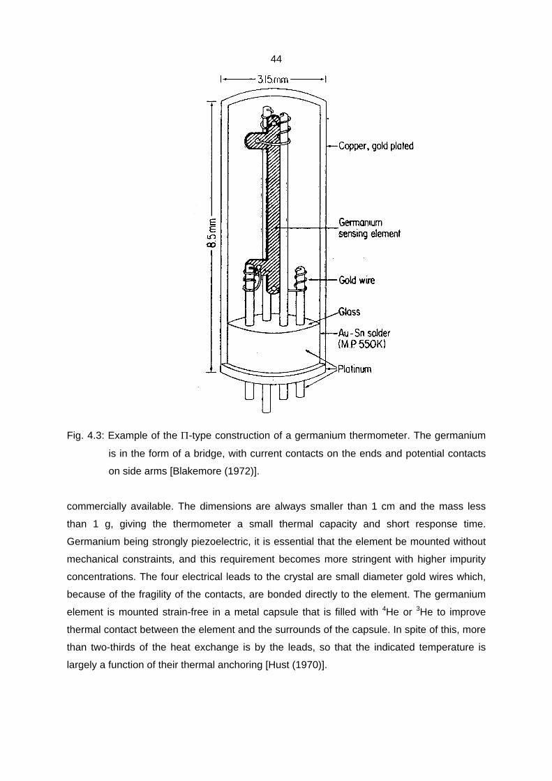
Fig. 4.3: Example of the Π-type construction of a germanium thermometer. The germanium

is in the form of a bridge, with current contacts on the ends and potential contacts

on side arms [Blakemore (1972)].

commercially available. The dimensions are always smaller than 1 cm and the mass less

than 1 g, giving the thermometer a small thermal capacity and short response time.

Germanium being strongly piezoelectric, it is essential that the element be mounted without

mechanical constraints, and this requirement becomes more stringent with higher impurity

concentrations. The four electrical leads to the crystal are small diameter gold wires which,

because of the fragility of the contacts, are bonded directly to the element. The germanium

element is mounted strain-free in a metal capsule that is filled with 4He or 3He to improve

thermal contact between the element and the surrounds of the capsule. In spite of this, more

than two-thirds of the heat exchange is by the leads, so that the indicated temperature is

largely a function of their thermal anchoring [Hust (1970)].

45

4.3 Electrical Characteristics 4.3.1 Method of Measurement The thermometer resistance is measured either by a potentiometric method or with a

resistance bridge. The lead resistances, inherent to the construction of the thermometer, are

of the order of 20% to 40% of that of the thermometer itself at a given temperature, and vary

with T in the same manner. These can cause systematic temperature-dependent errors

associated with the shunting effect of the large-but-finite input impedances of ac bridges.

Such errors do not occur with a potentiometer [Swenson and Wolfendale (1973)].

With germanium thermometers, differences occur between the results of ac and dc

measurements [Swenson and Wolfendale (1973), Kirby and Laubitz (1973), Anderson and

Swenson (1978), and Anderson et al. (1976)]. Resistances measured with alternating

current are always smaller than with direct current at a given temperature. This effect,

intrinsic to the thermometer and dependent upon its geometry, is due to the Peltier heating

and cooling at the current lead contacts to the germanium element. With continuous current

it produces temperature gradients between the two ends of the sensor resulting in the

development of a thermal emf between the potential contacts. For most applications where

millikelvin uncertainty is tolerable, either ac or dc calibrations can be used below 40 K, the

effect being of the same order as that due to typical self-heating (see Sec. 4.4.1).

Kirby and Laubitz (1973) on the basis of both a theoretical model and measurements

in the range 15 to 1500 Hz, show that the Peltier heating component is damped

exponentially with the exponent being proportional to √f. Since the error term is dependent

upon the positions of the potential contacts, there is also a difference in the magnitude of the

error between 2-lead and 4-lead thermometers. The magnitudes of the errors measured by

Swenson and Wolfendale (1973) agree roughly with those of Kirby and Laubitz (1973). The

differences between ac (30 Hz) and dc measurements with typical thermometers below 80 K

are shown in Fig. 4.4 [Anderson and Swenson (1978)]. The relative differences between ac

and dc measurement of resistance are roughly 0.7% at 300 K, 0.2% at 80 K, 0.02% at 50 K,

and 0.0001 % below 10 K, with any Peltier error being greater for the dc measurement. If not

compensated for, this corresponds to temperature errors of about 0.2 K at 100 K down to 0.1

mK at 20 K. If very precise measurements are needed, the model proposed by Kirby and

Laubitz (1973) allows prediction of the systematic errors providing one knows the thermal

conductivity and electrical resistivity of the germanium element and the Seebeck coefficient

of germanium relative to the material of the leads.

46

Fig. 4.4: Differences between dc and ac (30 Hz) calibrations for typical germanium

thermometers from Minneapolis Honeywell (upper hatched group, 250 to 1250 Ω

at 4.2 K), Lake Shore Cryotronics (lower hatched group, 500 Ω at 4.2 K), and

CryoCal (dashed curve, 500 Ω at 4.2 K) [after Anderson and Swenson (1978)].

4.3.2 Resistance/Temperature Characteristics and Sensitivity Typical examples of the variation of resistance (R) with T for commercial germanium

thermometers are shown in Fig. 4.5. The resistance at 1 K can be as high as 106 Ω and at

100 K as low as 1 Ω, but these are extreme values. For a typical thermometer suited to the

temperature range 1 K to 30 K, R ranges from 1000 Ω at 4.2 K to less than 10 Ω at 77 K.

The sensitivity (dR/dT) at 4.2 K is about -500 Ω K-1.

In practice the power dissipated in the sensor must be much less than 1 µW, corresponding

to a maximum current of 30 µA with a 1000 Ω thermometer, or a voltage across the sensor

of 30 mV (see Section 4.4.1 and Fig. 4.8). In order to measure temperatures near 4 K to

within 0.01 % (0.5 mK), that would require instrumentation having microvolt resolution. Even

lower sensor voltages are desirable, 2 to 4 mV being usual. Commonly, a potentiometric

method is used to measure the resistance because of the high resistances involved. At

every temperature the current is adjusted to maintain the voltage across the potential

terminals as high as compatible with self-heating. This allows one to take advantage of the

maximum sensitivity provided by the equipment. Where this procedure is inconvenient, a

constant measuring voltage can be used over a wide range and correction made for self-

heating (see Sec. 4.4.1).

47

Fig. 4.5: Some typical resistance versus temperature response curves for germanium

thermometers.

At very low temperatures the resistance can easily surpass 105 Ω so that the

measuring current will be of the order of tens of nanoamperes if the power dissipated is to

remain tolerable; the tolerable leakage current due to lack of insulation or from the

measuring instrument itself must be much smaller. That necessitates a measuring system

with excellent signal-to-noise ratio. The very large sensitivity and its rapid change with

temperature has both advantages (high precision of measurement) and disadvantages

(rather small practical temperature range for any one thermometer).

The complicated behaviour of R and dTdR

R1

as functions of temperature, resulting

from changes in the conduction mechanism in germanium, prevents their being expressed

by simple functions. On the other hand, since both the resistivity and its temperature

coefficient are strongly influenced by doping, one can obtain thermometers especially

adapted to particular uses. For example:

- n-doped thermometers have a relatively smoothly-changing sensitivity, and so a fairly wide

temperature range.

48

- conversely, p-doped thermometers are preferred for use in narrow temperature ranges

within which the resistance can be represented precisely by a relation of the form In R =

f(In T) (see Sec. 4.5). The limits of the temperature range can be chosen by suitable

control of the doping which, in turn, controls the temperature at which the conduction mode

changes (the hump in curve b in Fig. 4.2).

The value of R becomes inconveniently large at very low temperatures. It can be

reduced by changing the doping, so it is possible in principle to have a thermometer with

100 Ω resistance at 0.1 K, but manufacture becomes more difficult [Halverson and Johns

(1972)]. Also, the high magnetoresistance of germanium is often restrictive (see Chapter 17).

4.3.3 Stability Individual germanium thermometers can exhibit good stability, but many do not.

Instabilities are generally not large enough to be significant in applications where an

accuracy within 10 mK at 20 K is sufficient. For experiments where ± 0.05% uncertainty in

temperature is tolerable one can have confidence in the stability of the initial calibration.

Some detailed measurements of instability by Plumb et al. (1977), Besley and Plumb

(1978), and Besley (1978), (1980) on about 80 thermometers from 3 manufacturers have

shown that a considerable variation in instability occurs during thermal cycling between 20 K

and room temperature. Thermometers maintained at a constant temperature can be

remarkably stable (much better than 1 mK) but, of course, this type of situation would

represent an extremely rare application. After thermal cycling, a variety of types of instability

occur, ranging in magnitude from less than a millikelvin to tens of millikelvins. Some

thermometer resistances drift slowly but regularly; some can be relatively stable, then jump

abruptly by large amounts; some remain stable after a jump but others jump back; some are

generally erratic.

It is not possible, a priori, to select stable thermometers. Thermal cycling 10 to 30 times

consistent with the eventual use of the thermometer (i.e. rapid cycling if the thermometer will

undergo rapid temperature changes; slow cycling otherwise) should routinely be used to

detect many unstable ones, but it is not guaranteed that all will be detected. It is obviously

useful (and not especially costly) to conserve several of them for periodic intercomparisons

with working thermometers so as to identify unstable thermometers. Clearly, also, several

thermometers should be used together.

49

The causes of instability have not been definitively elucidated. There is some suggestion that

n-type germanium may be more stable than p-type. However, much of the instability,

especially the abrupt jumps, is associated with mechanical shocks; the attachment of the

leads to the germanium crystal is particularly vulnerable to damage. Thus it is highly likely

that instabilities are geometrical in nature (due especially to change in the geometry of the

lead arrangement) and are not caused by fundamental changes in the resistivity of the

element. A one-temperature recalibration will not recover the original calibration of an

unstable thermometer.

4.3.4 External Influences a) Hydrostatic pressure: No change larger than 0.1% in resistance for pressures up to 2 x

105 Pa has been observed [Low (1961)].

b) Radio frequency fields: Electromagnetic fields in the frequency range 30 to 300 MHz

can have a considerable effect on semiconductor thermometers. In the temperature

range 70 K to 300 K this can cause a relative error in ∆T/T of up to 30% [Zawadzki and

Sujak (1983)] that varies with frequency and temperature (see Fig. 4.6). Unfortunately,

the electromagnetic field strengths for which these data were taken were not reported.

At lower temperatures the effect is equally important, but detailed measurements of the

magnitude of the error are unavailable. However, at 4 K for example, the thermometer

resistance can increase 0.3% in the field of a nearby television transmitter. Obviously,

radio frequency shielding is necessary, and the thermometer should be placed

perpendicular to the electrical field. For work down to 1 K and germanium thermometer

resistances up to 105 Ω, special precautions are normally unnecessary. Occasionally,

however, a thermometer will have a rectifying lead, leading to an extremely noisy off-

balance signal. In such a case the thermometer must be discarded.

c) Magnetic fields: see Chapter 19.

4.4 Thermal Properties 4.4.1 Self-heating and Thermal Anchoring The passage of current can, by Joule heating, raise the temperature of the sensor

above that of the medium in which it is immersed. The increase in temperature is proportional

to the Joule heating and inversely proportional to the thermal resistance between the

thermometer and the medium. Figure 4.7 shows typical values of the magnitudes of the

50

Fig. 4.6: Effect of a radio-frequency electromagnetic field on the response of a germanium

thermometer. Curves 1-6 are for external fields of frequency 149 MHz, 170 MHz,

no field, 100-200 MHz, 300 MHz, 63 MHz respectively [after Zawadzki and Sujak

(1983)].

Fig. 4.7: Calibration errors due to self-heating for a germanium resistance thermometer for

both constant current and constant voltage operation [Anderson and Swenson

(1978)].

51

effect on temperature measurements under various conditions, indicating that operation at

constant voltage rather than at constant current is preferable. As long as the Kapitza

resistance can be neglected, the effect varies linearly with the power dissipated and depends

upon the effectiveness of the thermal exchange with the environment. When the voltage drop

across the potential leads is kept constant, the temperature change due to self-heating varies

roughly linearly with temperature below 30 K (Fig. 4.7), independent of thermometer

resistance. Rather than calculate powers when the current is changed, it is simpler to maintain

a constant voltage and use Fig. 4.7. This is a useful technique when, for example, determining

how much self-heating can be tolerated in calorimetric measurements. Another (related) rule-

of-thumb can be deduced from Figs. 4.5 and 4.7: for many germanium thermometers, the

electrical characteristics are such that δT/T ~ -1/2 δV/V, and so the sensitivity is roughly 1

µV/mK.

Figure 4.8 shows the self-heating observed in a large group of thermometers [Besley and

Kemp (1977)]. It can be used for any particular thermometer to estimate the self-heating after

the values at two or more points have been found. To limit the effect to 1 mK at 4 K, the power

dissipated must be less than 0.2 µW for a thermometer immersed in liquid helium and less

than 0.02 µW if it is immersed in helium vapour. The quality of the thermal anchoring can be

estimated through the experimental determination of the self-heating effect.

In order to ensure good thermal contact between the thermometer and the body whose

temperature is to be measured, several general rules should be followed that depend

essentially upon the geometric configuration of the interior of the cryostat. One of the simplest

is to provide a well or hole just large enough to accommodate the thermometer so

Fig. 4.8: Range of values of self-heating observed with a variety of germanium thermometers

[Besley and Kemp (1977)].

52

that it will not be subject to mechanical constraints, and to fill the remaining gap with a suitable

material that allows good heat transfer, such as one of a variety of greases, motor oil, Wood's

metal, etc. Anything containing a solvent that can damage the sheath or its seals (which may

be an epoxy) should be avoided and, as well, the material should be oxide-free. It is also

essential to thermally anchor the leads to the body, or to a shield maintained at the

temperature of the body. The leads should be of small diameter ≤ 0.1 mm), electrically

insulated, and a considerable length should be attached to the body with, for example, varnish

or nail polish [Hust (1970)]. Generally, the largest thermal leak is via the leads.

4.4.2 Time Constant The value of the time constant depends upon the temperature, the environment, the

thermal contact with the environment, and the thermal conductivity of the sheath, lead wires,

and other components of the thermometer. It can only be measured in situ. Some typical time

constants for germanium thermometers of various types under different conditions are given in

Table 4.1 [Blakemore (1972), Halverson and Johns (1972)]. Note that the dimensions and

masses of the thermometers do not account for all of the time constant variations. On abruptly

cooling a thermometer from 300 K to 4.2 K, about 20 s is required for the thermometer to

reach equilibrium.

The time constant increases with temperature because of the rapid increase of the

thermal capacity of the thermometer with respect to the thermal conductivity. To minimize the

time constant of a germanium thermometer one must ensure that the lead wires are properly

thermally anchored as near as possible to the thermometer itself.

4.5 Calibration and Interpolation Formulae

A description of the resistance/temperature characteristics of germanium resistance

thermometers is not possible by simple formulae based on theoretical considerations. As the

characteristics can be very different from thermometer to thermometer, individual calibrations at

a large number of points are necessary. To approximate the characteristic with the minimum

possible uncertainty from the experimental data, a suitable fitting method has to be used.

Furthermore, the calibration itself should already take into account any peculiarities of the fitting

method [Powell et al. (1972)]. The results and conclusions in the literature concerning the

efficiency of various fitting methods are obscure and, in some cases, contradictory because

53

Table 4.1: Typical Time Constants in Helium Liquid and Vapour for Various Germanium

Thermometers.

Time Constant (s) Manufacturer Thermometer Time Constant in helium vapour Characteristics (s) in liquid at 1.27 cm above helium the liquid level ________________________________________________________________________ Scientific Mass 0.081 g Instruments Length 4.75 mm 0.010 0.180 type p- 1000 Ω at 4.2 K Diameter 2.36 mm _________________________________________________________________________ CryoCal type CR1000 Mass 0.290 g type n- 857 Ω at 4.2 K Length 11 mm 0.03 0.200 Diameter 3.1 mm _________________________________________________________________________ Honeywell type II Mass 0.5 g (at 3 cm) (circa 1963) Length 11 mm 0.05 0.38 Diameter 3.5 mm

- only in a few cases are different methods compared directly;

- the results obtained are valid only for the individual thermometer types

investigated;

- the uncertainties of the input data are very different in the various papers;

- some questions (for example weighting and smoothing with spline functions)

are not sufficiently investigated;

- the mathematical bases are often incompletely described.

Hence it is not possible to give here a recipe which can be applied in all cases. A

classification of the various least squares fitting methods with general remarks on their

efficiency was made by Fellmuth (1986), (1987). Only one method is recommended here; it

allows the characteristics of all germanium resistance thermometers mentioned in Appendix

C to be approximated in the temperature range from about 1 K to 30 K with high precision

(uncertainty less than 1 mK). The features of this method are:

(i) interpolation equations:

⎟⎠⎞

⎜⎝⎛=∑

= NM - R ln

AT lnn

0ii i (4.1)

54

⎟⎠⎞

⎜⎝⎛=∑

= SP - T ln

BR lnn

0ii i (4.2)

where R is the thermometer resistance, T is the temperature, M and P are origin-shifting

constants, N and S are scaling constants, and Ai and Bj are coefficients resulting from the

curve fitting.

(ii) approximation of the characteristic in two subranges which overlap several

kelvins (range of overlap about 5 K to 10 K)

(iii) value of n is about 12 for a range 1 to 30 K, but may be about 5 for the range 1 to

5 K for the same accuracy

(iv) number of calibration points greater than about 3 n, or 2 n if the distribution of

points is carefully controlled

(v) calibration points at nearly equal intervals in In T except near the ends of any

calibration range (and perhaps in the range of overlap), where there should be a

distinctly higher density of points. An ideal spacing is such that the m points are

distributed according to the formula

⎟⎠⎞

⎜⎝⎛+

+p

1-m1-i

cos2

x-x2

xx 1m1m , (i = 1 to m)

where x1 and xm are the lower and upper limits respectively of the independent

variable (In R or In T in equations 4.1 and 4.2 respectively).

Using this method, the errors introduced by spurious oscillations are comparable with the

uncertainty of the input data. For the selection of the optimum degree several criteria must

be applied (Fellmuth (1986), (1987)], which is easy if orthogonal functions are used.

It is possible that the number of calibrations points can be greatly reduced if the

general behaviour of the characteristic of the individual thermometer is known or if a larger

uncertainty is tolerable. Unfortunately, in the literature, only isolated data on this matter are

available. It must be emphasized that a direct application of literature techniques is only

possible if the same type of thermometer is used; and that special interpolation equations

can approximate the characteristics of particular types of thermometers sufficiently closely

with a lower degree than would result from application of Eq. (4.1) or (4.2), but their use can

cause considerable difficulty if these equations are not matched to the characteristic of the

individual thermometer to be calibrated.

55

5. Rhodium-Iron Resistance Thermometers

Rhodium-iron resistance thermometers were developed by Rusby (1972) for use

below the normal range of the platinum resistance thermometer. It was found that, of various

small concentrations of iron in rhodium, the one that would give the most sensitive and yet

moderately linear thermometer was 0.5 atomic percent iron [Rusby (1975)]. Rusby (1982),

who uses a group of them at the National Physical Laboratory to carry the primary

temperature scale below 30 K, has given a review of ten years of performance. Present

suppliers of rhodium-iron thermometers are listed in Appendix C.

5.1 Range of Use and Sensitivity The range of use is normally from about 0.5 K to 30 K, although the sensitivity is

good up to room temperature and at lower temperatures. For a capsule-type thermometer

containing helium gas, the lower limit of about 0.5 K is set by the rapidly-increasing self-

heating. The normal upper limit (~ 30 K) is in the region where the superior platinum

resistance thermometer has adequate sensitivity.

In contrast to pure metals, for which the sensitivity dR/dT decreases steadily with

decreasing T at small values of T, the sensitivity of rhodium with about 0.5% iron impurity is

relatively constant at about 0.4 Ω/K down to 100 K, decreases to ≤ 0.2 Ω/K near 25 K, then

increases rapidly by about a factor of 10 as T decreases to 0.5 K as illustrated in Fig. 5.1 for

a thermometer with an ice-point resistance of 100 ohm. The industrial type has a sensitivity

about 6% lower than the standard type. It is in this low temperature region of increasing

sensitivity that rhodium-iron has its chief application. The rapid change in sensitivity in the

low temperature region means that, to obtain a precision of 1 mK at 30 K, the rhodium-iron

resistance must be measured to 1 part in 105, compared to 10 in 105 for platinum. Because

the rhodium-iron resistance is much higher, however, the voltage sensitivity at 30 K is higher

than for platinum. The sensitivity of rhodium-iron is much lower than that of germanium.

5.2 Fabrication The standard-type thermometer of H. Tinsley and Co., Ltd. (U.K.) is constructed as

follows: the 0.05 mm diameter wire is wound in the form of coils inside four glass tubes

which in turn are encapsulated in a 5 mm diameter platinum sheath as shown in Fig. 5.2.

The sheath contains helium at about 1/3 atmosphere pressure. The leads are 0.3 mm

56

Fig. 5.1: Resistance (Ω) and sensitivity, dR/dT(Ω/K) , of a type 5187W rhodium-iron

resistance thermometer [after Rusby (1982)].

Fig. 5.2: Construction of a rhodium-iron thermometer of the high precision type. The coil of

wire is mounted inside four glass tubes, two of which are shown, b; the assembly

is inserted into a platinum sheath, a; 4 platinum leads are flame-welded to the

rhodium-iron wire, c; the sheath and the leads are sealed in an atmosphere of

helium by a glass bulb, d; [after Rusby (1975)].

57

platinum wire and the element is so mounted as to be strain free. Two versions are

available: one (type U) has about 50 Ω resistance at 273 K, is 27 mm long, with overall

length including a glass seal around the leads of 45 mm; the second (type W) has about

twice the resistance and is about 15 mm longer. The 50 Ω thermometer has a resistance of

about 3.5 Ω at 4.2 K.

Oxford Instruments Ltd. supplies two industrial types: Type R3 (R(0 °C) = 20 ohm) is

mounted in a vented stainless steel body, 25 mm long and 3.2 mm in diameter. In type R4

(R(0 °C) = 27 ohm) the coil is mounted in four cylindrical chambers of an alumina body 22

mm long and 3.2 mm in diameter. Inside each of these chambers is a layer of a very high

temperature glass that bonds a part of each loop of the alloy coil to the alumina body. The

latter model is intended for use from cryogenic temperatures up to 700 °C.

More recently Cryogenic Consultants Ltd. have achieved success in producing thin-

film rhodium-iron thermometers [Barber et al. (1987)]. The thermometric material is sputtered

on to a sapphire substrate. For films between 0.5 µm and 1.0 µm thick the sensitivity is

similar to or slightly higher than that of wire-wound thermometers, and variation of resistance

with temperature is very similar to that for wire-wound thermometers. Thinner films have

lower sensitivities. Ice-point resistances are in the same range as those of wire-wound units.

Thin-film thermometers are now available commercially.

5.3 Reproducibility and Stability More than ten years of study have shown that rhodium-iron thermometers have

excellent long term stability. For the standard-type, Rusby (1982) reports that for five

thermometers, after at least 50 cycles between 273 K and 20 K, the average shift was 0.2

mK and the largest 0.35 mK (in 8.5 years). The latter corresponds to a resistance change of

60 µΩ or 5 parts in 106 of the resistance. At 4.2 K no shifts larger than ± 0.05 mK were

observed. This is at the level of uncertainty of the measurements themselves. Also for the

standard-type, Besley (1982) describes similar excellent performance: 9 thermometers were

cycled 30 times from 293 K to 6 K and 8 were completely stable; the ninth showed only a

small change < 0.1 mK at 6 K and 1 mK at 90 K).

Only a limited amount of information is available on the stability of the industrial type.

Besley (1984) examined three of the ceramic-type units. After 20 cycles between 20 K and

room temperature, stability was almost within the precision of the measurements,

i.e. 1 ± 0.3 mK. However, handling (such as by repeated soldering of the

58

thermometer wires) caused a more remarkable change of resistance, equivalent to as much

as 3 mK at 2.1 K and 16 mK at 30 K. This apparently was due to relief of strain in the wire

and seems to limit the stability of this model.

A limited number of thermal cycling tests on thin-film thermometers indicate that

stability to within ± 2 mK is achieved after about 15 cycles between room temperature and

4.2 K, about twice the number of cycles as required for the wire-wound industrial type

[Barber et al. (1987)].

5.4 Self-heating Self-heating has been found to be closely the same for both U and W standard-type

thermometers; its magnitude is shown in Fig. 5.3 for currents of 0.1 and 0.3 mA. Near 1.5 K

the self-heating falls dramatically as the 4He filling of the capsule condenses to superfluid

liquid and thermal contact is vastly improved. As the temperature further decreases, self-

heating rises rapidly again. Self-heating in thin-film thermometers is generally smaller than in

wire-wound ones.

Fig. 5.3: Typical self-heating effect for a 4He-filled rhodium-iron thermometer with measuring

currents of 0.1 mA and 0.3 mA [Rusby (1982)].

5.5 Calibration and Interpolation A rhodium-iron thermometer is normally calibrated at many points in the range of

interest and the data fitted by least squares as described for germanium. The equation

chosen is usually of the form

59

(5.1) ∑=

=n

0i

ixa T i

where x = AR + B, and B and A are origin-shifting and scaling constants respectively that

change the range of the independent variable to -1 ≤ x ≤ 1. For a wide range such as 0.5 K

to 27 K, n ~ 10 is necessary if fitting errors are to be ~ 0.2 mK. For lesser precision or

narrower ranges, lower degree can be used - typically n = 4, 8, 9 for ranges 0.5 K to 4.2 K,

20 K, 24 K respectively. For temperatures above 27 K, R is usually replaced by In R or In Z

(where Z is defined by Eq. (8.5)) in Eq. (5.1). If a change in calibration occurs, it is possible

to account for it by expressing the calibration data in terms of Z with the two calibration

points (for Z) near the extremities of the range.

Another equation, requiring fewer calibration points, has been found to fit calibrations

of 25 thermometers satisfactorily [Rusby (1982)]:

in

0ii )] T[ln(b R τ+=∑

=

(5.2)

For τ of the order of 8 to 10 K, the standard deviation of the residuals is less than 0.3 mK for

n = 6 and where the points are weighted by dT/dR. Equation (5.2) is of special interest

because it allows interpolation in the range from 0.5 K to 25 K using calibrations at a

restricted set of easily realizable temperatures - helium vapour pressures, superconductive

transitions, and triple and boiling points.

The characteristics of rhodium-iron are such that the constants of the interpolation

equation do not vary greatly from thermometer to thermometer from the same batch of wire,

in contrast to germanium for which they vary widely from one to another.

From the limited information available on the industrial-type thermometer [Besley

(1985)], it appears that the ceramic type may approximate the ITS-90 in the range 77 K to

273 K to within about 10 or 25 mK using a reference function together with a deviation

function that requires 2 or 3 calibration points respectively.

60

6. Vapour Pressure Thermometry*

Vapour pressure thermometers are based on the saturated vapour pressure in a two-

phase system in an enclosure. A boiling point is an example of a point on a vapour pressure

curve; i.e. the techniques of vapour pressure thermometry described herein apply also to the

special case of a boiling or a triple point determination. The behavior of a liquid-vapour

system in equilibrium, for example, is describable by an equation P = f(T) (curve tC of

Fig. 6.1). Along the curve for a pure substance, the pressure depends on the temperature

and not on the quantity of substance enclosed or vaporized. The temperature range

associated with vaporization is limited to temperatures between the critical point and the

triple point of the substance. The range is even further reduced if the extreme pressures to

be measured are outside the usable range of the pressure sensor.

For a given substance, the sensitivity of the thermometer increases approximately

inversely with the temperature since uv varies roughly as 1/P (curve tC in Fig. 6.1).

According to the Clausius-Clapeyron equation, we have

)uu(TL

dTdP

Lv −=

where L is the molar heat of vaporization which is temperature dependent, and uv and uL are

the molar volumes of the saturated vapour and liquid respectively. Experimental tables

giving P = f(T) have existed for a long time for commonly-used fluids and interpolation

formulae have been internationally agreed upon for many of them [Bedford et al. (1984)]. It is

therefore easy to obtain temperature from measurement of pressure.

The sublimation curve can be similarly used, but the range of measurable

temperatures is then much smaller, limited on the high side by the triple point temperature

and on the low side by the pressure becoming too low to be measured accurately enough.

Here, the discussion emphasizes thermometers based on liquid-to-vapour

_________________________________________________________________________

* This chapter is written in more detail and contains rather more of the fundamentals of the

theory than other chapters because no self-contained account of vapour pressure

thermometry appears elsewhere, vapour pressure thermometry is one of the best means

of approximating the ITS-90, and the techniques are moderately commonly used

industrially.

61

Fig. 6.1: Schematic phase diagram for a pure substance (t is the triple point and C the

critical point.

Fig. 6.2: Vaporization curve for a mixture of two pure substances: ACA, saturated

vapour pressure curve of pure substance A; BCB, saturated vapour pressure

curve of pure substance B; GC, critical point of the mixture; CACB, locus of the

critical points of the mixture as a function of overall composition.

62

transitions, but it could be applied also to those based on solid-to-vapour transitions

(sublimation) with suitable changes.

6.1 Two-Phase Equilibrium The number of parameters that can be arbitrarily imposed on a system is given by

Gibb's phase rule:

v = c + 2 - Φ

where c is the number of constituents of the system, Φ is the number of phases, and v is the

number of degrees of freedom (or variance). For a pure substance with two phases (c = 1,

Φ = 2), v = 1. The data for the pressure therefore fix the value of the temperature at the

intersection in Fig. 6.1 of a line T = constant with the curve tC; this is the measurement

principle of the thermometers described here. In fact, the points of this curve are a series of

equilibrium states that are distinguished by the distribution between the two phases of the

total number of moles of the substance enclosed.

The equilibrium is regulated by the Gibbs-Duhem relationship, which holds in the

simple case described here, by the simultaneous realization of three conditions:

PL = Pv TL = Tv and µL(TL,PL) = µv(Tv,Pv) ,

where the indices L and v refer to the liquid and vapour phases respectively; P and T are the

pressure and temperature at the separation surface; and µ, the chemical potential, is

identical for a pure substance to the free molar enthalpy. Any variation of one of the three

quantities causes displacement of the equilibrium.

If the substance is not pure but contains soluble impurities, the variance of the

system, becomes equal to the number of constituents present. Suppose that: each

constituent is present at the same time in both liquid and vapour phases; the vapour phase

is a mixture of perfect vapours; the surface-tension is negligible; the liquid phase is an ideal

solution, that is to say, the substances mix without change of volume or enthalpy. This last

assumption is realistic so long as the molar fractions xi (i = 2 to n) of the (n - 1) impurities

present (solutes) are very small with respect to that (x1 ~ 1) of the pure substance (solvent)

filling the thermometer. (Note that the respective concentrations denoted xiL and xi

v (i = 1 to

n) are generally not equal, as will be seen later.) Under these conditions, the deviation

63

from an ideal solution is less than 1 % so long as the molar fractions of solutes are less than

10-3.

The equilibrium of such a system must always satisfy the Gibbs-Duhem relation; that

is, each constituent must have the same chemical potential in the two phases: µiv = µiL for

i = 1 to n. The chemical potential is a function of pressure, temperature, and molar fractions

of constituents.

The influence of the impurities present is as follows:

a) At temperature T, the pressure P above the liquid is different from the saturated vapour

pressure Π1 of the pure substance since it is equal to the sum of the partial pressures pi of

the various constituents (Dalton's Law): i.e.

PxpPn

1i

vi

n

1ii ⋅== ∑∑

==

This can be used to determine the calibration errors of the apparatus.

b) At temperature T, the saturated vapour pressure Π i of a pure substance is higher than the

partial pressure pi of this substance in the mixture:

pi = xiL Π i (Raoult's Law) .

For the solvent, for which xiL ~ 1, we can write:

1

n

2i

Li1

L11 x1xp Π

−=Π= ∑

=

For a weak concentration of solute (xiL → 0) it is necessary to replace the above

expression by

pi = xiL ki (Henry's Law) ,

where ki (≠ Π i) is a constant that depends on the temperature and the nature of the

constituents present.

As a result of the above, the quantity of every dissolved impurity is proportional to its

own partial pressure. We can write

64

[∑=

−Π−Π=n

2ii1

Li1 kx ]P ,

where the total pressure is a linear function of the concentrations of impurities in the liquid.

The second term will be greater than or less than zero according as the impurities are more

or less volatile than the solvent. The boiling temperature of a solution with a given

concentration is not that of the pure substance at the same pressure.

In Fig. 6.2 showing a mixture of two components, the vaporization curve of pure

substance A is ACA and that of pure substance B is BCB. The critical point of the mixture is

somewhere on the dashed curve CACB, depending upon the concentrations of the two

components. If it is at C, the vaporization of the mixture takes place on the solid curve.

Referring to Fig. 6.2, at the temperature T the pure substance boils at pressure Π1. The

solution boils at the partial pressure p1, less than Π1, since

∑=

=Π−Π 2

2i

Li

1

11 xp

Suppose the total pressure above the solution is P. At this pressure A would boil at TA and B

at TB. If the solvent A is more volatile than the solute B, the solution begins to boil at T' > TA.

In the opposite case (solvent B less volatile than solute A), the closest the boiling

temperature of the solution comes to TB is T", obtained at the end of vaporization or the

beginning of condensation (dew point).

c) The concentration of impurities is different in the two phases and changes during the

course of vaporization. We can write:

Px

Ppx i

Liiv

iΠ

==

(Π i being replaced by ki if xi → 0) ,

so that 1

iL

1

Li

v1

vi

xx

xx

ΠΠ

⋅= for all i = 2 to n . (6.1)

Suppose again there are two constituents. If 1 is more volatile than 2, i.e. if

65

. x xand , x xthat so , xx

xx then , L

2v

2L

1v

1L2

L2

v1

v2

21 <><Π>Π

Thus the vapour is always richer than the liquid in the more volatile constituent. A useful

method to detect impurities is to compare the boiling temperatures for two different fillings of

the bulb. If the total quantity of impurities is constant, the pressure for a given temperature

will depend upon the level of liquid. The result deduced immediately following Eq. (6.1) may

also be used for purifying a substance by withdrawing vapour during boiling. Conversely, if

the impurity (constituent 1) is less volatile than the solvent (constituent 2), this procedure will

increase the concentration of impurities in the solution.

For a given pressure P, we can trace figuratively the evolution of the system in Fig.

6.3a. For simplicity, suppose once more there is only one type of impurity (x2 = 1 - x1 ) . Two

cases occur depending upon whether constituent 2 is more or less volatile than

constituent 1. Let T1 and T2 be the boiling temperatures of pure substances 1 and 2 at

pressure P. Suppose first T1 > T2 (i.e. impurity more volatile than solvent). If we cool a

sample of vapour with concentration x2v = x, a drop of liquid will appear at temperature

TA < T1 when the dew point is reached. The impurity concentration in this drop of liquid is

x2L = x' < x, corresponding to point B. The temperature TA obtained is the closest to T1 that

can be reached starting from the vapour concentration x2v. As the temperature continues to

decrease, the condensation continues along the curve B → C until all the gas is liquified at

point C with temperature TC < TA, and with a concentration x2L = x.

Conversely, with increasing temperature, the point C is attained first; the temperature

the closest to T1 is obtained at the end of the vaporization.

An analogous reasoning in the case of an impurity less volatile than the solvent shows that

the temperature closest to T 1 will be obtained at the beginning of the vaporization (Fig.

6.3b).

If there are many types of impurities, some more volatile and others less volatile than

the solvent, the reasoning becomes more complicated, and an experimental study is more

profitable.

The above examples concern ideal solutions that can exist only if the constituents

present have very similar properties. This approximation is made for a mixture of isotopes or

for sufficiently dilute impurities. It becomes complicated for insoluble impurities that are

present only in the vapour phase or for substances that have several

stoichiometric forms with change of abundance ratios during vaporization. Moreover,

66

Fig. 6.3: Diagram at constant pressure of a two-phase mixture (1, liquid; 2, liquid-

vapour; 3, vapour): (a) T1 > T2, impurity more volatile than solvent;

(b) T2 > T1, impurity less volatile than solvent.

67

impurities with densities different from that of the pure substance can create concentration

gradients in the liquid phase; the preceding reasoning is then valid only near the surface of

separation.

This shows the necessity of selecting an easily purifiable substance for use as a

vapour pressure thermometer.

6.2 Technical Details of Construction A vapour pressure thermometer essentially consists of: a bulb containing the pure

measuring substance in thermal equilibrium with the sample whose temperature is to be

measured; a pressure sensor; a connecting tube long enough to connect the bulb to the

pressure sensor; and a valve for filling (Fig. 6.4).

6.2.1 Bulb The bulb can be very small depending upon the quantity of substance necessary to

cover the required temperature range. It is necessary to ensure that at no time during

temperature cycling the substance reassembles into a single phase. The maximum pressure

that will occur determines the thickness of the walls of the bulb. The bulb is formed from a

material that is a good heat conductor, is chemically neutral, and neither absorbs nor

desorbs gases. It is thermally anchored into a copper block which also contains the sample

whose temperature is to be measured. If the thermometer is intended to measure the

temperature of a large body, the bulb is most often an elongated cylinder (for an industrial

thermometer, typically 120 mm long by 15 mm diameter, giving a volume ~ 20 cm3), but its

shape can vary as required. For example, if it is intended to calibrate resistance

thermometers, those sensors are located within the walls of the bulb.

The quantity of filling substance is determined by the necessity to ensure that the

surface between the two phases be in the bulb and not in the connecting tube. Moreover, as

we have seen, the temperature changes during boiling according to the nature of the

impurities. Referring to Figs. 6.3a and 6.3b, we note that the bulb should contain relatively

little substance if the impurities are more volatile than the solvent, and should be almost

completely filled with liquid if the impurities are less volatile than the solvent.

The bulb's form is dictated by the necessity to take account of eventual concentration

gradients caused by impurities in the liquid phase. If the enclosed substance is a poor

conductor of heat in the condensed phase, e.g. non-superfluid helium, the interior of the bulb

is so structured that no large thickness of the substance can become the centre of a

temperature gradient. An example of a device used for calibration of germanium resistance

thermometers is shown in Fig. 6.5 [after Moser and Bonnier (1972)].

68

Fig. 6.4: Schematic construction of a saturated vapour pressure thermometer: 1, bulb

containing two phases of a substance; 2, pressure sensor; 3, connecting

tube; 4, filling system.

Fig. 6.5: Bulb of a helium vapour pressure thermometer [Moser and Bonnier (1972)]:

1, 4He; 2, connecting tube; 3, radiation trap; 4, jacket; 5, thermometer well;

6, thermal leak; 7, differential thermocouple; 8, resistance heating;

9, conduction cooling.

69

6.2.2 Connecting Tube Because the pressure sensor is usually at room temperature, the connecting tube

must bea poor heat conductor; long enough to limit the contribution of heat due to the

temperature gradient; equipped with a radiation trap to avoid direct radiation heating of the

separation surface between the two phases; small enough that its volume is small compared

to the volume of vapour in the bulb to prevent a large change in the liquid/vapour ratio; of

cross section sufficient to limit thermomolecular effects and to avoid blocking. It is necessary

to avoid creating a cold spot in the connecting tube where the enclosed substance can

condense to form a drop of liquid that blocks the tube (although with helium such a cold spot

does not form (it is self-quenching) [Ambler and Hudson (1956)] (see also Sec. 6.3.7)). Then

the pressure measured would correspond to the temperature of the cold spot. This latter

difficulty can be avoided by placing the connecting tube inside an evacuated tube (Fig. 6.6)

and/or imposing a small heat flow along the connecting tube. The temperature gradient so

created must be controlled (Fig. 6.5) and accounted for as a correction to the measurement

results. For example, for a stainless steel connecting tube of 1 m length, internal diameter

2 mm, and external diameter 2.5 mm between 300 K and the helium temperature, the heat

flux is about 6 mW (0.8 mW with glass), a heat leak which could produce a temperature

difference of 3 mK between the bulb and the liquid helium.

The inner diameters used are generally 0.5 to 3 mm unless thermomolecular effects

are likely to arise.

6.2.3 Pressure Sensor The sensor is chosen according to the temperature range and the precision required.

For an industrial thermometer it is most often a Bourdon gauge, or a mercury or oil (or any

substance having small vapour pressure) manometer, used with a cathetometer. For high

precision measurements, one can also use a Bourdon quartz spiral gauge periodically

calibrated against a pressure balance. A diaphragm pressure transducer is also used, giving

a signal that can be amplified and handled by a computer. It can be placed very close to the

evaporation surface, which reduces many problems related to the connecting tube (Fig. 6.7),

but then there are problems in calibrating it.

Whatever pressure sensor is chosen, its internal volume must be small (see

Appendix D) and the metrological characteristics of the thermometer will be determined by

the manometer. If the substance used in the thermometer is corrosive, the pressure can be

transmitted across a membrane or incompressible liquid.

70

Fig. 6.6: Use of an evacuated jacket to avoid a cold spot in a helium vapour pressure

thermometer [Cataland et al (1962)].

Fig. 6.7: Illustration of the use of a capacitive sensor with a vapour pressure

thermometer [Gonano and Adams (1970)]: A, sensor sheet; B, diaphragm; C,

capacitor plates; D, insulating feedthrough; E, insulating ceramic tube; F,

bellows; G, bulb.

71

6.2.4 Filling the Thermometer Before filling the bulb it is important to analyze the filling substance for the nature and

quantity of impurities, to clean the enclosure with suitable chemicals or solvents, to bake it

above 100 °C if possible, and to flush the enclosure several times with the filling substance

to avoid contamination. When filling the thermometer, one must be certain that the volumes

of the bulb, connecting tube, and manometer are compatible with the temperatures to be

measured. To obtain the required quantity, it is necessary to include an extra reservoir (see

Fig. 6.8); for example, one litre of liquid helium at normal pressure occupies 746 litres when

it is transformed into the vapour phase at room temperature under normal pressure. The

necessary details to determine the quantity of the substance at the pressure and

temperature of filling are given in Appendix D.

Fig. 6.8: Schematic drawing of an installation for filling a vapour pressure

thermometer.

The filling proceeds as follows: after flushing and evacuating of the installation, the

ensemble is filled under pressure P; on closing the inlet valve for the filling gas, the desired

quantity is condensed into the bulb at temperature Tf and the pressure evolution followed

until it reaches Pf. This can take a very long time because of the low thermal conductivities of

the gas in the connecting tube and of the connecting tube itself [Van Mal (1969)]. The time is

proportional to the length and diameter of the tube (30 min for a diameter of 5 mm and

length of 50 cm for helium between 300 K and 4 K).

72

Following this, the connecting tube, bulb, and manometer are isolated from the

remainder of the installation (see Fig. 6.8).

6.3 Metrological Characteristics and Measurement Corrections 6.3.1. Extent of Sensitivity and Measurement Many substances could be used as a vapour pressure thermometer. The only

constraint is to obtain a sufficient purity. The response curves P = f(T) of some substances

are shown in Fig. 6.9. For each substance the temperature range is restricted. In the

cryogenic domain, there are three temperature zones that are not covered: below 0.5 K (all

pure substances have too low a vapour pressure), between 5.22 K and 13.81 K, and

between 44.4 K and 63.15 K. These zones could be partially covered by sublimation vapour

pressure thermometers. (Sublimation for nitrogen is possible between 56 K and 63.146 K

[Bedford et al. (1984)] and for hydrogen between 10 K and 13.81 K). The response curve is

usually an empirical relation of the form

...CTTBA

ppln0

++−= (with p0 = 101325 Pa)

For 3He and 4He, vapour pressure equations were derived for the EPT -76 by Durieux et al.

(1982) and Durieux and Rusby (1983). Inverted forms (T = f(P)) were subsequently

produced by Rusby and Durieux (1984), and these are now included in the ITS -90. For

other substances (H2, Ne, N2, Ar, O2, S) the coefficients are given by Bedford et al. (1984).

The sensitivity of vapour pressure thermometers can be high, especially the higher

the pressure, and this is one of their advantages.

6.3.2 Reproducibility and Accuracy The reproducibility of a vapour pressure thermometer is essentially determined by

the pressure sensor. The actual magnitude of the imprecision is dependent upon the

particular manometer; as typical examples, for a mercury manometer between 233 000 Pa

and 6 600 Pa, the imprecision can be ≤ 1.3 Pa; for an oil manometer with p < 6 600 Pa, the

imprecision is 0.09 to 0.18 Pa.

The excellent intrinsic reproducibility (10-3 to 10-4 K for helium, 10-2 to 10-3 K for other

cryogenic fluids) has led to vapour pressure thermometers being used to define some

thermometric scales. In particular, 3He and 4He gave birth to T62 and T58 respectively

[Sydoriak and Sherman (1964) and Brickwedde et al. (1960)]. Later, with

73

Fig. 6.9: Equilibrium vapour pressure curves for some substances used in saturated

vapour pressure thermometers. The crosses on each curve are the triple

point (lower) and the critical point (higher). (a) 3He, 4He; (b) normal H2 and D2

and Ne;

74

Fig. 6.9: (c) N2, CO, Ar, O2, CH4; (d) Ar, O2, CH4, CO2, C2H6, C3H8, CCl2F2, C2H6O,

C4H10, H2O.

75

some corrections, these scales served to extend the IPTS-68 to lower temperatures and to

form part of the EPT-76 [Durieux et al. (1982)], and are now incorporated as part of the

definition of the ITS-90.

Although the vapour pressure thermometer is an excellent secondary thermometer, it

can only measure thermodynamic temperatures with many corrections and uncertainties and

by using empirical values for the parameters.

6.3.3 Response Time The time constant of a vapour pressure thermometer is essentially a function of that

of the pressure sensor, of the thermal contact between the bulb and the object whose

temperature is to be measured, and of the thermal diffusivity of the liquid. Certain particular

configurations can make the time response very long.

6.3.4 Correction for Aerostatic Pressure

When the connecting tube is long, it is necessary to correct for the weight of the

enclosed vertical vapour column. The correction requires a knowledge of the distribution of

the temperatures because of the density variation in the connecting tube; it therefore

depends upon the design and can be rather inaccurate (see Appendix E). The correction

depends essentially on the part of the connecting tube which is close to the bulb.

For oxygen at the boiling point (~ 90 K) the pressure correction in a vacuum-jacketed

sensing tube about 50 cm long is about 1 Pa, equivalent to a temperature correction of

1.3 mK. The uncertainty of the correction due to the inability to measure or predict the true

temperature of the gas is at least 0.2 mK [Compton and Ward (1976), Kemp et al. (1976),

Ancsin (1973a)]. For a 1 metre connecting tube containing helium joining room temperature

to bulb temperature, Moser and Bonnier (1972) calculated corrections of 0.1 mK and 0.03

mK for bulb temperatures of 4.2 K and 2 K, respectively. The aerostatic correction may be

determined with a 1 % uncertainty using an auxiliary tube [Klein et al. (1979)], but the

procedure is difficult.

If possible, it is preferable to use a horizontal tube, or to pass the connecting tube

through an isothermal enclosure, thus reducing the effects of a temperature gradient.

6.3.5 Thermomolecular Effect There exists in the connecting tube a thermomolecular pressure gradient between

the hot (higher pressure) and cold (lower pressure) extremities that is sizeable when the

mean free path of the molecules is not much smaller than the tube diameter, e.g. for 4He

around 1 K. When the effect is not measured, one usually corrects for this gradient using

76

the Weber-Schmidt equation [Weber et al. (1936)], although also the experimental tables of

Roberts and Sydoriak (1956), or the calculation of Bennett and Tompkins (1957) can be

used for the two helium isotopes. The Weber-Schmidt equation is

9930.4y9930.4y ln 15823.0

8311.1y8311.1y ln 41284.0

1878.0y1878.0y ln 18131.0

TT ln

21

PPln

2

1

2

1

2

1

2

1

2

1

++

−++

+++

+=

where ( ) n11.273/TX

RPy+

=

X = 1.8087, n = 0.147 for helium,

X = 1.1470, n = 0.195 for hydrogen.

Index 1 indicates the hot end of the tube, index 2 the cold end; R designates the tube

radius in cm, P the pressure in Pa, and T the temperature in K.

The trend of the effect is shown in Fig. 6.10 [Roberts and Sydoriak (1956), Durieux et

al. (1982)].

Some temperature values for a vapour pressure thermometer using He or H2 are

shown in Table 6.1

With oxygen, the correction reaches 20 mK near 54 K (when P = 100 Pa), but it is

already less than 0.05 mK at 64 K for an Inconel tube 1.6 mm in diameter [Tiggelman

(1973)]. For neon near 20 K it is less than 1 mK [Tiggelman (1973)].

In general, these calculations can be 10% to 25% in error [McConville et al. (1966)

and McConville (1972)], since the correction depends upon the material used for the tube

and the physico-chemical conditions of its inner surface, which may also vary with time.

They can be calculated [McConville et al. (1966)] as a function of the reflection coefficient of

the tube but, unfortunately, the latter is never well known and may change after long

exposure to the gas.

The thermomolecular effect can be measured with an additional tube [Berry (1979)].

Another solution, which eliminates the correction, is to use a diaphragm transducer located

in the lower temperature region [Gonano and Adams (1970)] (see Fig. 6.7).

Current practice consists of using pressure tubes of the largest section possible

compatible with keeping heat transfer losses reasonably small (and to include some means

of blocking radiation (gains, not losses) and damping oscillations). If the calculated

correction is to be realistic, it is indispensable to have a constant diameter in the parts of the

tube where the temperature is ill-defined.

The two corrections from Secs. 6.3.4 and 6.3.5 are usually small and in many cases

the only significant uncertainty is that due to the reading of the pressure.

77

Fig. 6.10: Ratios of thermo molecular pressures for 3He and 4He (R, radius of tube in

centimetres; pF and pc, pressure in Pa at the cold (TF) and hot (Tc) extremities

of the tube) [Roberts and Sydoriak (1956)].

Fig. 6.11: The observed lowering of the vapour pressure of N2 by nonvolatile impurities,

as a function of the vapour pressure of pure N2. Curve A, N2:100 ppmv. CO;

curve B, N2:100 ppmv. Ar; curve C, N2:100 ppmv. Kr; curve D, N2:100 ppmv.

O2 [Ancsin (1974a)].

78

Table 6.1: Temperature values (K) at the cold extremity of the connecting tube of a

vapour pressure thermometer using helium or hydrogen for various tube

diameters, a hot extremity at room temperature, and thermomolecular effects

of 10 mK and 1 mK.

Filling Thermomolecular Tube Diameter (mm) gas Effect 0.5 1 5 10 ___________________________________________ 3He: dT = 10 mK 0.76 0.65 0.48 0.42 K dT= 1 mK 1.08 0.90 0.64 0.56 K 4He: dT = 10 mK 1.45 1.30 1.05 0.96 K dT= 1 mK 1.83 1.62 1.27 1.16 K

H2: dT = 10 mK below 10 K dT = 1 mK below 10 K

Table 6.2: Amounts by which small Concentrations of 3He in liquid 4He affect Vapour

Pressure.

Concentration of Temperature (K) Pressure Equivalent 3He (%) Change (kPa) Temperature Change (K) _________________________________________________________________________

0.12 1.5 1.6 0.5

0.02 1.5 0.3 0.2

0.12 2.6 5.2 0.2

0.02 2.6 0.6 0.04

_________________________________________________________________________

79

6.3.6 Corrections Due to Impurities

a. Helium (3He, 4He)

The only impurity problem with helium is isotopic since all other substances are solid

at these temperatures and the solids are not soluble in liquid helium.

The presence of 4He in liquid 3He lowers the vapour pressure below that of pure 3He.

The concentration of 4He in the vapour phase is much less important than in the liquid

phase. For concentrations of 4He in the liquid phase of < 10%, we can use [Sydoriak and

Sherman (1964)] the approximate formula (derived from Raoult's Law)

( ) ( )dx

P lndx1P xx −=−Π

In this expression x is the concentration of 3He (> 90%); Π is the saturated vapour pressure

of pure 3He and Px is the pressure of the mixture at temperature T; the derivative is taken for

x = 1 at temperature T. One can obtain correction curves at the calculated temperatures

according to this formula [Sydoriak and Sherman (1964)]. For 0.1 % of 4He in the liquid

phase, this gives a temperature correction of 0.02 mK at 0.4 K and of 0.71 mK at 3.2 K.

In 4He, the only awkward impurity would be 3He. Commercially supplied 4He contains no 3He, so the only risk of error would be from its accidental introduction from, e.g., poor

manipulation of a dilution refrigerator. Not many measurements have been made, but they

are confirmed by theoretical calculation. Even a small concentration of 3He in 4He causes a

considerable increase in the vapour pressure, as shown in Table 6.2. The numerical values

in the table concern the concentration of 3He in the liquid phase of 4He. The concentrations

of 3He in the vapour phase are even more important than in the liquid phase.

b. Hydrogen [Ancsin (1977)]

The only volatile impurity, He, seems not to be soluble in liquid hydrogen and is

therefore not in contact with the separation surface. Other impurities are condensed and

cause no problem except for Ne which can cause errors up to ∆P = 210 Pa (∆T = 1 mK) at

19 K for a concentration of 410 ppm in volume.

Other errors can occur because the ortho-para conversion of hydrogen is not

instantaneous and the proportion of these two states is a function of the temperature. At

room temperature, normal hydrogen is 75% ortho and 25% para, while at 20 K equilibrium

hydrogen is 0.21 % ortho and 99.79% para with a boiling point 0.12 K lower than that of

normal hydrogen. To obtain reproducible results, one must introduce a catalyst

80

into the bulb (hydrous ferric oxide). It should be enclosed in a metallic mesh to avoid its

dispersing to the walls during boiling. The quantity of catalyst is not important (e.g. 0.15 g)

but it is inefficient if it is not in good contact with the liquid phase.

There are similar problems with deuterium, which is more easily contaminated, and

always contains some hydrogen deuteride (HD) even after the most careful preparation. HD

will also be formed in measurable quantities (over 1%) from hydrogen atoms that diffuse

from the bulk of the container or, more commonly, from exchange with H2O if a hydrated

catalyst is used. Errors of several hundredths of a kelvin may arise near 18.7 K [Pavese and

McConville (1987)].

c. Neon [Ancsin (1978), Furukawa (1972), Tiggelman et al. (1972), Tiggelman (1973)]

The volatile impurities, H2 and He, are not soluble in the liquid phase and do not

influence the vaporization curve. Their presence in the vapour phase causes a decrease in

the boiling temperature of Ne. Their effect can be minimized by increasing the volume of the

vapour phase [Ancsin (1978)].

Most of the possible nonvolatile impurities have small partial pressures below 27 K

and are trapped somewhere in the tube. Only nitrogen has a notable influence. The limit of

solubility of N2 in Ne is 150 ppmv*. The triple point temperature of saturated Ne is 2.25 mK

lower than for pure Ne. For a mixture with 1000 ppmv* of N2, the vapour pressure is lowered

by 100 to 300 Pa, giving a boiling temperature 6 to 10 mK higher than pure Ne between

24.562 K and 27.102 K.

It appears that the isotopic constitution of natural neon varies so little from one

supplier to another that there is no need to be concerned with variations in it. Natural neon

as described in "Supplementary Information for the ITS-90" [CCT (1990)] is composed of

90.5% of 20Ne, 0.27% of 21Ne, and 9.2% of 22Ne. The 21Ne is in too small a quantity to

influence the results, but this is not the case for 22Ne and 20Ne which have different boiling

and triple points: the latter are 24.546 K and 24.687 K respectively (corresponding to a

pressure difference of 326 Pa). An increase of the concentration of 20Ne by 0.1% increases

the normal boiling point by 0.13 mK.

There also exists an isotopic composition difference between the liquid and vapour

phases. The molar concentration of 22Ne is higher in the liquid phase than in the vapour

phase by 0.3% at the boiling point and 0.4% at the triple point [Furukawa (1972)]. This

_________________________________________________________________________

* The abbreviation ppmv is used to mean an impurity content of one part by volume of

solute per 106 parts by volume of solvent.

81

creates an uncertainty of 0.4 mK in the value of the normal boiling point depending upon

whether the ITS composition applies to the liquid or the vapour phase. In the absence of a

precise analysis, the error can be minimized if the volume of the liquid phase is much larger

than that of the vapour phase.

d. Nitrogen [Ancsin (1974a)]

For nitrogen in the liquid phase, volatile impurities such as He, H2, and Ne, if present,

stay entirely in the vapour phase and have no detectable effect on the temperature of the

boiling liquid. Non-volatile impurities such as O2 and Ar lower the triple point value, while CO

and (especially) Kr raise it.

Impurities have a complex effect on the whole vapour pressure relationship, which

cannot simply be represented as a shift proportional to the temperature changes at the triple

and normal boiling points (Fig. 6.11). There is a consequent change of all the constants in

the vapour pressure equation.

e. Argon [Ancsin (1973b)]

As impurities, He, Ne, and H2 have no influence; N2 (volatile) decreases the

temperature of the dew point by more than 2 mK for 100 ppmv. Oxygen (nonvolatile) has no

influence if the concentration is less than 200 ppmv, whereas CH4 and Kr (nonvolatiles)

increase the dew point temperature by approximately 2 mK for 100 ppmv.

f. Oxygen [Ancsin (1973a, 1974b), Tiggelman (1973), Compton and Ward (1976), Kemp et

al. (1976)]

Since the principal impurities are volatile it is necessary to use a well-filled bulb.

Helium and neon are not soluble in liquid oxygen. For a concentration of 1 ppmv, nitrogen

decreases the boiling (condensation) point temperature by 19 µK; krypton increases it by

5.6 µK; argon decreases it by approximately 5 µK. The influence of H2O and CO2 is

imperceptible up to a concentration of 100 ppmv.

As observed with nitrogen, the effect of the impurities on the whole vapour pressure

curve is highly non-linear, and therefore distorts the whole vapour pressure equation (Fig.

6.12) [Ancsin (1974b)]. Some of the discrepancies observed in the literature between

different vapour pressure scales can be attributed to this effect.

The isotopic effects in oxygen are perceptible only when the volume of residual liquid

is small. The vapour pressure of pure 18O is about 1.5% less than that of the "normal"

mixture; the associated correction is about 11 µK at the boiling point for an isotopic

composition of 0.210% instead of 0.204% [Tiggelman and Durieux (1972b)].

82

Fig. 6.12: Effect on the vapour pressure of oxygen due to the indicated volatile

impurities as a function of temperature. Curve A, O2:1000 ppmv. N2 V (vapour

phase) = 1.61; curve 8, O2:1000 ppmv. Ar V (vapour phase) = 1.61; curve C,

O2:100 ppmv. N2 V (vapour phase) = 0.41; curve D, O2:100 ppmv. N2 V

(vapour phase) = 1.61 [Ancsin (1974b)].

83

6.3.7 Particular Problems with Helium [Cataland et al. (1962), Kerrik (1970), Montgomery and Pells (1963), Rusby and Swenson (1980)]

Information on the realization of helium vapour pressure scales is available in

"Supplementary Information for the ITS-90" [CCT (1990)]. As for other substances, it is

necessary to avoid the formation of cold spots which can cause an error in reading. In 4He,

such a cold spot can be at the same level as the liquid surface. In fact, He I above the λ-

point (2.1768 K) has a very low thermal conductivity so temperature gradients can occur,

especially near the surface if evaporation is taking place. Below the first 4 millimeters, the

temperature variation under static (non-convective) conditions would be equal to that of the

hydrostatic pressure (0.14 mK/cm at 4.2 K; 0.27 mK/cm at 3.34 K; 1 mK/cm at 2.2 K). Nearer

the surface, the effect depends upon the cryostat design; at 4.2 K a temperature increase of

up to 5 mK above the surface temperature in the first 4 mm has been observed [Durieux

(1960)]. The vapour temperature above the surface is therefore lower by several mK than

that of a body immersed just below the surface. The vertical gradient can cause an error of

up to 20% of the measured temperature if the temperature of an immersed body is deduced

from the pressure in the vapour phase and accounted for only with the hydrostatic

correction. This temperature gradient, detectable by the appearance of bubbles in the center

of the liquid, depends also on the rate of evaporation. It is necessary to use a well-insulated

dewar and to fractionate the liquid mass with fins or massive braids to improve the thermal

contact with the surface of the bulb (Fig. 6.5). Rather than measure the pressure just above

the liquid in which the body whose temperature is required is immersed, one can also use a

small auxiliary bulb in good thermal contact with it. The pressure tube must then cross the

liquid-vapour surface in the dewar and it is there that there is a risk of a cold spot forming,

although according to Ambler and Hudson (1956) this is unlikely (see also Sec. 6.2.2). A

vacuum jacket around the capillary tube will suffice to avoid this cold spot but it must not

reach to room temperature which would make thermal isolation difficult (Fig. 6.6). A heat flux

along the wall of the internal tube must also be avoided; if it cannot be otherwise controlled,

some copper foil in the bath and surrounding the capillary would prevent the formation of

temperature gradients. In summary, large and unquantifiable temperature gradients can

arise in bulk He I and therefore a bulb should be used.

Below 2.1768 K He II is an excellent thermal conductor so the temperature gradient

does not exist. On the other hand, being a superfluid, He II climbs along the bulb walls,

vaporizes, and returns to the liquid surface. This produces a heat input to the bulb by

refluxing because the superfluid film does not carry away entropy, so the entropy density of

84

the remaining liquid increases. The large Kapitza resistance is also troublesome. The

temperature of the liquid can be many millikelvins higher than that of the walls (15 mK to 1.5

K). This phenomenon can be corrected for (but not reliably) by calculation, and can be

reduced by increasing the surface of the bulb/liquid contact up to several hundreds of cm2

(metal mesh or spirals of copper in the bulb). Furthermore, the viscosity of the return gas

induces a pressure gradient in the capillary which can become important below 1 K.

Note that if these problems are not under control, the measured temperatures will be

discontinuous at the λ-point. For precise measurements, the error due to the Kapitza effect

(which can be about 4 mK at 1.5 K) is too important to ignore [Lounasmaa (1974) for

temperatures below 1 K; Wilks (1967) for higher temperatures]. It can be calculated, or it can

be avoided by using 3He, which does not become superfluid, instead of 4He in the

temperature range where the two scales overlap; for 4He one should always use a bulb

above the λ -point, and always measure the bath pressure directly below the λ -point. Below

the λ -point the refluxing and Kapitza effects can be avoided by measuring the vapour

pressure a short distance up the pumping tube [Rusby and Swenson (1980)].

6.3.8 Other Corrections Other corrections to be considered in pressure measurements include: expansion of

the mercury of the manometer and variation of its density with the temperature; the shape of

the meniscus; hydrostatic pressure correction (if we measure the temperature of a body

immersed in the liquid). The latter can be uncertain but can usually be kept small because

the depth of liquid is seldom large.

6.4 Conclusion The vapour pressure thermometer can be used as a thermodynamic thermometer

only within the limits of application of the Clausius-Clapeyron equation which result from lack

of knowledge of several of the parameters. Otherwise it is an excellent practical thermometer

based upon a physical property of a pure substance. Simple and practical, it allows a high

measurement precision once the pressure-temperature relationship has been established.

The bulb is simple to construct and can be very small. There are not many corrections to

apply (a few for impurities possibly, but no dead space corrections as in the gas

thermometer). The major inconveniences are its small working range (no pure substance

covers a large temperature range) and its nonlinearity of response. The development of new

pressure sensors may give renewed interest in vapour pressure thermometers.

85

7. Magnetic Thermometry

7.1 Magnetic Thermometer Magnetic thermometry is based upon measurement of paramagnetic susceptibility.

Useful papers concerned with the EPT-76 temperature range are Rusby and Swenson

(1980); Cetas and Swenson (1972); van Rijn and Durieux (1972); Cetas (1976); Mangum

and Bowers (1978). For an ideal paramagnet the zero-field susceptibility is related to

temperature through the Curie law χ = C/T where C is the Curie constant. Although in

magnetic thermometry one approximates to this by using dilute paramagnetic salts, it is

generally necessary to take account of interactions and other effects and write

χ = C/(T + ∆ + γ/T), where ∆ includes first-order dipole-dipole and exchange couplings and

also a shape factor, while γ is due primarily to crystal field splitting of the ground state and

second-order interaction effects [Hudson (1972)]. The existence of interactions implies a

lower limit for the use of any given salt, while the upper limit is set by diminishing sensitivity

(dχ/dT is approximately equal to -C/T2). The susceptibility measurement is usually made by

the ac mutual inductance method in which the salt sample is situated in a set of coils whose

mutual inductance M is balanced against a reference in a Hartshorn bridge or a variant

thereof [Hudson (1972)] (SQUlD techniques do not appear to have been applied much

above 1 K). The bridge balance X is linearly related to M and hence to χ. The working

equation for a magnetic thermometer becomes

X = A + B/( T + ∆ + γ/T) (7.1 )

Unless ∆ or γ is obtainable from theory, a minimum of four fixed points is needed to calibrate

the thermometer.

Salt crystals must be grown carefully from ingredients of high purity. Most of the

suitable salts are hydrates and almost all of these are efflorescent, tending to lose water-of-

crystallization if kept at room temperature. This tendency is considerably diminished if the

enclosing volume is small and is filled with an inert gas; but it is catastrophically increased if

the enclosure is evacuated. Simple refrigeration, however, avoids most such problems. The

properties of the most important salts have been widely discussed and tabulated

[e.g. Hudson (1972)]. Cerous magnesium nitrate (CMN) is the closest approximation to an

ideal paramagnet in common use: γ = 0 and for a sphere ∆ is about 0.3 mK. It is, however,

highly anisotropic and its usefulness is limited to temperatures below 3 K because of its low

86

Curie constant (C⊥ is about 0.011 K in SI units referred to unit volume) and the existence of

an excited state which becomes significantly populated at higher temperatures [Rusby and

Swenson (1980)]. Another rare-earth salt, neodymium ethylsulphate (NES), is less

anisotropic and about four times stronger than CMN. It has been used successfully between

2 K and 16 K [Mangum and Bowers (1978)] and there appears to be no bar to using it down

to 0.5 K or lower [Hudson (1972)].

Chromic methylammonium alum (CMA) is a salt of intermediate strength (C being

about 0.077 K) which has been used for the range 1 to 20 K [Cetas and Swenson (1972);

Durieux et al. (1962)]. Manganous ammonium sulphate (MAS) [Cetas and Swenson (1972);

Cetas (1976); Durieux et al. (1962)], and gadolinium sulphate (GS) [Cetas (1976); Durieux et

al. (1962)] are classed as strong, with C about 0.26 K and 0.79 K respectively, and they are

therefore more suitable if the range is to extend to 30 K. Another possibility is gadolinium

metaphosphate (GP) [Mangum and Bowers (1978)], which has the practical advantage of

being anhydrous, but for all of these strong salts ∆ and γ would have to be determined in the

experiment using at least four fixed points, and the lower limit for accurate use might not be

below 2 K.

7. 2 Technical Aspects of Magnetic Thermometry For the simple case of a primary solenoid of m turns per metre and a secondary of

turns-area product nA wound on it, the mutual inductance M is µµ0mnA. If the coils contain

a salt with a geometrical filling factor f, then ∆ = (1 + fχ) and if χ = C/T the sensitivity dlnM/dT

is approximately - fC/T2. For f = 0.5 and C = 0.26 K as for MAS, one therefore requires a

precision ∆M/M of 2 parts in 107 if 1 mK is to be resolved at 25 K.

With a primary current ip of angular frequency ω the solenoidal field H is Mip and the voltage

across the secondary is ipωM or µµ0HnAω. The design of the thermometer and bridge must

be such that this is large enough to achieve the desired sensitivity. Typically µ0H might be

0.1 to 0.3 mT without departing seriously from the zero field limit, and the frequency is

usually between 30 and 300 Hz. Taking 0.2 mT and 100 Hz and a secondary of 500 turns on

a radius of 1 cm, the voltage would be 0.02 volt, 2 parts in 107 of which is 4 nV. This is not

unreasonable, but there is need for caution and the design should aim to provide greater

sensitivity than is indicated by such calculations. While the product nA can be gauged in

advance, the frequency and field may be limited by the effect of eddy currents (roughly

proportional to ω2H) induced in nearby metallic components. To combat them,

87

glass and plastic materials should be used where possible, and the coil system should be as

well separated from the thermometer block as is practicable. Good heat transfer may be

achieved through varnished copper wires, but tests of their effectiveness should be

undertaken. Various other precautions could include [Cetas and Swenson (1972)] using a

quadrupolar configuration of secondary coils, and shielding the coil system with

superconductive Pb sheeting. The latter reduces external interference and ensures that eddy

currents are independent of metallic resistivities and hence are independent of temperature.

As regards the measurement technique, it is standard practice to include in the

cryostat a set of empty coils identical to those surrounding the salt, with the secondaries

connected in opposition. Then the net mutual inductance is small and relatively insensitive to

extraneous magnetic and electrical interference. Suitable mutual inductance bridges with

adequate sensitivity can be assembled using commercially-available measuring equipment.

An essential preliminary to magnetic thermometry is a check of the performance of

the bridge and coil system in the absence of the salt. After the system is cooled from room

temperature, the bridge balance should first be checked for stability at a constant

temperature for a period of hours during which time any dependence on primary current,

coolant liquid level, exchange gas pressure, room temperature, or disturbance to the

cryostat should be tested. Then the bridge balance should be monitored as a function of

block temperature in order to establish the background effects at all currents to be used. If

these effects are not small, steps should be taken to reduce them or at least to ensure their

reproducibility from one assembling of the coils to another.

Only when the background has been satisfactorily characterized should a salt be

mounted and magnetic thermometry begin. Again, the stability of the measuring system

should be monitored after initial cooling. Bridge balance and thermometer resistance may

then be measured at many temperatures in the range, with enough time allowed at each

temperature to reach equilibrium. It is advisable to make measurements at more than one

value of the primary current and to check for drifts in the bridge balance by returning to the

starting temperature at the end of a measurement session. It may help the analysis if there is

some overlap between data taken in different sessions, particularly after an overnight

interval or a transfer of liquid helium or nitrogen. After correction for bridge drifts and

background effects, the unknown constants are evaluated from the measurements taken at

the chosen reference temperatures, and values of T90 at intermediate temperatures are

calculated.

88

8. Platinum Resistance Thermometers 8.1 General Remarks

The platinum resistance thermometer (PRT) is very widely used below 500 °C as a

thermometric sensor. There is a wide range of quality of PRT available, from the standard

instrument (SPRT) of the ITS-90 to some industrial types (IPRT) that are accurate only to

within a few tenths of a kelvin or, perhaps, even a kelvin or more. The major difference of the

industrial type of fabrication from the standard type is not just the purity of platinum, but also

the less strain-free mounting of the film or wire which is embedded (partially or totally) in a

cement (glass or refractory). Furthermore, in most cases, the thermometer body is not

hermetically sealed.

The ITS restricts the quality of the thermometer that may be used as a standard

instrument. For the ITS-90 an acceptable PRT must be made from pure, strain-free platinum,

and it must satisfy at least one of the following two relations:

W(29.7646 °C) ≥ 1.118 07

W(-38.8344 °C) ≤ 0.844 235 ,

where W(t90) = R(t90)/R(0.01 °C)*. If the PRT is to be used to the freezing point of

silver, it must also satisfy the relation

W(961.78 °C) ≥ 4.2844 .

These relations are closely equivalent to the restriction that

(dW(t90)/dt90)0.01 °C ≥ 3.986 x 10-3 K-1 .

These relations, in essence, assure that the platinum in an SPRT is highly pure. They are

equivalent to the requirement that W(H20 b.p.) > 1.392 44, whereas it is estimated that

_________________________________________________________________________

* Note that this definition of W(t90) is different from the equivalent one for W68(t68). The

latter uses R(0 °C) as the reference in the ratio. It follows that W68(t68) = 1.000 040 W(t90)

to better than 1 part in 106 for any SPRT.

89

for ideally pure platinum W(H20 b.p.) ~ 1.392 74. No such restrictions apply, in principle, to a

PRT used to approximate the ITS-90. Various national and international bodies place

restrictions on the quality of PRT that is suitable to meet their requirements for accuracy, the

restriction taking the form of a specification on W(H20 b.p.). In addition, in conjunction with

the use of standard tables of resistance, the value of R(0 °C) is specified. Also, the

resistance ratio W(4.2 K) is sometimes used as a quality indicator. The most accurate

thermometers (corresponding to W(H20 b.p.) > 1.3925 have W(4.2 K) < 4 x 10-4, whereas

industrial thermometers (corresponding to W(H20 b.p.) ~1.385) have W(4.2 K) nearer

2 x 10-2. It must also be remembered that for industrial purposes the platinum sensing

element is usually mounted within a protective sheath which can modify some of the

characteristics of the sensor itself. It is the latter that has been most often studied in the

references to follow.

In Section 8.2 we outline a few simple methods for approximating the ITS-90* based

upon fixed-point calibrations and simple interpolation formulae to be used with SPRTs, with

indications of the accuracies that may be achieved. Discussion of IPRTs is given in Chapter

16 in Part 2.

8.2 Interpolation Equations for Standard Platinum Resistance Thermometers* The approximations described here are concerned with SPRTs calibrated with

simplified methods for medium to high accuracy. Several such simplified procedures have

been suggested but only some of the more promising of them are described here. Some of

the others appear either to be too complicated or to have been insufficiently tested (e.g. too

few thermometers) to be suitable for recommendation.

(a) Perhaps the simplest secondary realization is an extrapolation below 273 K of the

following defining equations of the IPTS-68 from above 273 K:

−

°

−

°

−

°

°+= 1

C 74.630't1

C 58.419't1

C 100't

C 100't045.0'tt 68 (8.1)

W68(t') = 1 + At' + Bt'2 (8.2)

_________________________________________________________________________

* All of these methods were devised as approximations to the IPTS-68 but they are also

applicable to the ITS-90.

90

For a group of 45 thermometers having W68(H20 b.p.) > 1.3925, Bedford (1972b)

showed that if the thermometers were calibrated only at the triple and boiling points

of water and if a common value of B were assumed for every thermometer, then the

extrapolated temperatures (Te) diverge smoothly from T68 (or T90) by up to 1 K at 100

K, 1.7 K at 70 K, and -12 K near 20 K, and variations in these temperatures are small

(Fig. 6.1). Using a tabulated or functional correction, one can measure T68 (and,

consequently, T90 using the tables of Appendix A) to within ± 3 mK down to 150 K, ±

15 mK at 77 K, and ± 30 mK at 30 K. We note that:

(i) The method is simple. The thermometers are calibrated only at the triple

and boiling points of water. If B were measured by a tin-point or zinc-point

calibration, the extrapolated scale uncertainty might be marginally smaller.

This would be feasible for a long-stem thermometer but not for many

capsule thermometers.

(ii) The procedure is equally valid for capsule or long-stem PRTs.

(iii) There is no definitive test of the extrapolation; there is a high probability,

but no certainty, that any particular PRT will fall within the uncertainties

quoted.

(b) Another simple secondary realization for the range 90 K to 273 K uses only two fixed

points and obtains a third from an experimentally-observed linear correlation between

W(O2 b.p.) and W(H20 b.p.). This correlation was first pointed out by Brodskii (1968),

who found the following relation for thermometers with W68(H20 b.p.) > 1.3920:

W(O2 b.p.) = a1 + b1 (W(H20 b.p.) -1) . (8.3)

Berry [(1963), (1972)] examined similar correlations in detail. For platinum of the

highest available purity, he determined [Berry (1972)] a linear relation of the form of

Eq. (8.3) corresponding to various equilibrium concentrations of quenched-in

vacancies. This is shown as curve V in Fig. 8.2, which Berry suggested would be an

upper bound for all real PRTs. Similarly, his curve L [Berry (1963)] approximates the

mean behaviour for his large group of thermometers. From Fig. 9 of Berry (1963) one

can deduce a lower bound (curve M) below which no SPRT is likely to lie.

91

Fig. 8.1: Differences from T90 of temperatures Te extrapolated below 0 °C using the

IPTS-68 defining equations for above 0 °C. The hatched area shows the

maximum observed deviations ∆(T90 - Te) in (T90 - Te) for a group of 45

thermometers [Bedford (1986)].

Fig. 8.2: Linear relationships between W(O2 b.p.) and W(H20 b.p.) for platinum: B, after

Brodskii (1968); V, ideally pure platinum [Berry (1972)]; L, mean of many

thermometers [Berry (1963)]; M, lower bound for SPRT [Berry (1963)]; S,

result when argon replaces oxygen, converted to oxygen [Seifert (1980),

(1984)]; [Bedford (1986)].

92

More recently, Seifert [(1980), (1984)] considered a relation similar to Eq. (8.3)

relating W68(Ar t.p.) to W68(H20 b.p.):

W68(H20 b.p.) = -0.525 29 W68(Ar t.p.) + 1.506 108 (8.4)

Using the WCCT-68(T68) ratio of 1.128 402 for W68(O2 b.p.)/W68(Ar t.p.), Seifert's

equation can be converted to the form of Eq. (8.3); the result is shown as curve S in

Fig. 8.2. Curve S has a more negative slope than the others and rises above V at

lower values of W(H20 b.p.). The coefficients a1 and b1 of Eq. (8.3) are given in Table

8.1 for all of the curves in Fig. (8.2).

Table 8.1: Coefficients a1, b1 of Eq. (8.3) for the Curves in Fig. (8.1).

_________________________________________________________________________

Curve a1 b1 reference

_________________________________________________________________________

B 0.977 86 -1.870 0 Brodskii (1963)

V 0.982 826 -1.882 572 Berry (1972)

L 0.903 485 -1.680 508 Berry (1963)

M 0.779 641 -1.365 254 Berry (1963)

S 1.087 070 -2.148 156 Seifert (1980), (1984)

_________________________________________________________________________

Equation (8.3) allows a secondary realization from 90 K to 273 K with calibration at

only the triple point of water and the boiling point of either oxygen or water, the other being

estimated from Eq. (8.3). The coefficients a1, b1 for curve L are probably the most

representative. Used with the IPTS-68 defining equation for the range 90.188 K to 273.15 K,

this secondary realization is probably accurate to within ± 30 mK when W(H20 b.p.) ~ 1.3920

and ± 10 mK when W(H20 b.p.) > 1.3925. In Eq. (8.3), W(O2 b.p.) could be replaced with

W(Ar t.p.) and W(H20 b.p.) by W(ln f.p.) (with suitable adjustment of the coefficients a1 and

b1), and an equivalent accuracy would result. According to the finding of Bedford (1972b),

extrapolation to about 70 K will produce little further degradation in accuracy. Although

temperatures between 125 K and 273 K are less sensitive to an error in W(O2 b.p.) than in

W(H20 b.p.), it is probably better and usually more convenient to calibrate at

93

the oxygen or argon point and deduce the resistance ratio at the steam point.

Moreover, few laboratories now maintain a steam point, and most capsule

thermometers cannot safely be heated as high as the tin freezing point, another

reason to prefer calibration at the oxygen point and deduction of W(H20 b.p.). As

indicated by Seifert, a relation similar to Eq. (8.3) based upon the argon triple point is

even better. It obviates the need for any boiling-point measurement, requiring only

two simple triple-point determinations. Seifert (1984) has extended this method by

using one- or two-point comparisons with a standard PRT (at, e.g., 160 K and 78 K)

to replace the argon-triple-point measurement. The accuracy is little degraded

thereby.

(c) Several possibilities for secondary realization based upon Cragoe Z-functions rather

than simple resistance ratios have been proposed. Among early investigations were

those of Cragoe (1948), Corruccini (1960), (1962), and Barber (1962). The Z-function

is defined by

)T(R)T(R)T(R)T(R)T(Z

12

1

−−

= , (8.5)

where T1 and T2 are fixed-point calibration temperatures at or near the extremities of

the range. The Z-function for a particular choice of calibration temperatures is

tabulated and temperatures are calculated by interpolating deviations from the table

in some specified way. The Z-function tabulation acts as a reference function

equivalent to Wr(T90). Besley and Kemp (1978) incorporate the Z-function into a

reference function using T1 = 4.2 K (boiling helium) and T2 = 273.15 K (melting ice) in

Eq. (8.5). They define a reference function of the form n16

0nn 54.3

54.3)Zln(A*T

+=∑

=

(8.6)

using the mean value of Z of a group of 19 thermometers each with W(4.2 K) < 4 x

10-4. Temperature (T = T* - ∆T*) is determined for any particular thermometer in

terms of a deviation from Eq. (8.6) of the form

T K 40*T1 a*T

2/1

∆

−=∆ , (8.7)

where ∆T = b + c W(4.2 K) + d W(4.2 K)2 , T* ≤ 40 K (8.8)

and ∆T = 0 . T* > 40 K (8.9)

94

For thermometers with W(4.2 K) < 4 x 10-4 this scheme allows calibration of

thermometers to within ± 0.02 K from 14 K to 273 K.

Using the same method for a group of 31 thermometers having 4 x 10-4 <

W(4.2 K) < 7 x 10-4, but using a different reference function (in place of Eq. (8.6)) and

correction polynomial (in place of Eq. (8.8)), Besley and Kemp (1978) obtained an

accuracy within ± 0.02 K above 40 K for 31 thermometers, and within ± 0.04 K below

40 K for 29 thermometers.

In summary, the thermometer is calibrated only at 4.2 K and 273.15 K. A

temperature T is obtained by measuring R(T), calculating Z(T) from Eq. (8.5),

calculating T* from Eq. (8.6), and calculating ∆T* from Eqs. (8.7) - (8.9). When

4 x 10-4 < W(4.2 K) < 7 X 10-4, the procedure is similar, but uses different reference

and correction polynomials. With this proposal:

(i) only a relatively simple 2-point calibration is required,

(ii) only SPRTs are likely to have W(4.2 K) < 4 X 10-4,

(iii) it is not applicable to long-stem thermometers; to measure any temperature

below 273 K, a calibration at 4.2 K is necessary,

(iv) there is no test for the accuracy of interpolation for any particular

thermometer.

(d) Several other useful approximations to the ITS have been described (see the original

papers for details). Kirby et al. (1975) proposed a single deviation function from 14 K

to 273 K determined by calibration against a previously-calibrated SPRT at four

points using three boiling liquids (He, H2, N2) and the ice point; the resulting

inaccuracy is about ± 10 x 10-6 in W. Pavese et al. (1978) suggested using the same

equations as in the IPTS-68 but a different set of fixed points that included only triple

points. Tiggelman and Durieux (1972a) showed that a polynomial in the form

∑=

=6

0n

nnTA)T(W (8.10)

can fit 14 calibration points between 2 K and 15 K with a standard deviation of ±

2 mK at 4.2 K decreasing to ± 0.3 mK above 11 K for 10 high quality SPRTs (W(H20

b.p.) > 1.3926). In the range 4 - 15 K a mere five points allow an accuracy of ± 3 mK.

95

9. Platinum Thermocouples 9. 1 General Remarks

Thermocouples employing platinum in combination with platinum-rhodium alloys,

gold, or palladium have been found to be the most reproducible of all the various types. They

are resistant to oxidation in air and, because of their high melting points, can be used up to

very high temperatures. The best-known member of this group is Pt10Rh/Pt* (or type S, or

10/0). It was long considered more accurate and has probably been studied more than any

other thermocouple; moreover, and presumably for these reasons, it served as a defining

instrument in the ITS-27, the IPTS-48 and the IPTS-68. It is not one of the defining

instruments of the ITS-90, its role having been taken over by the SPRT. Any Pt10Rh/Pt

thermocouple, in order to qualify as a defining instrument for interpolation in the range from

630.74 °C to the gold point (1064.43 °C), had to meet strict requirements for purity and

thermocouple emf [CCT (1976)].

The Pt13Rh/Pt (or type R, or 13/0) thermocouple is very similar in its properties to the

type S; containing 13% Rh by weight, it has a little higher sensitivity and probably also a little

higher reproducibility.

In many situations the precision of types Sand R thermocouples, especially above

500 °C, is limited to about ± 0.2 °C. For more precise measurements Mclaren and Murdock

(1987) have shown that the gold/platinum thermocouple is clearly superior in stability,

homogeneity, and sensitivity (about twice that of type S). It even challenges the SPRT on the

basis of simplicity and economic practicality. With care, temperatures can be measured to

within ± 10 mK in the range 0 °C to 1000 °C. For higher temperatures the palladium/platinum

thermocouple has likewise shown considerable promise as being more accurate than type S

or R. Precision within ± 20 mK at 1100 °C and ± 50 mK at 1300 °C has been achieved.

Studies of both of these types are in progress.

The upper temperature limit of use for types R and S thermocouples in an oxidizing

atmosphere is quoted as high as 1600 °C (for 0.5 mm diameter wires). Better platinum-

rhodium alloy combinations for thermometry under oxidizing conditions above 1100 °C,

however, are Pt30Rh/Pt6Rh (or type B, or 30/6) or the non-standardized combinations

Pt20Rh/Pt5Rh (20/5) and Pt40Rh/Pt20Rh (40/20). These have proven to be exceptionally

stable and may be used continuously in air to 1700 °C. In one test, for example, after 200 h

heating at 1700 °C in air, the emf of the 20/5 thermocouples had decreased the equivalent of

about 5 K at the palladium point (1555 °C) [Bedford (1964)];

___________________________

* See footnote on page 6.

96

after 500 h at 1700 °C in air, the 40/20 thermocouples exhibited changes equivalent to 4 K at

the palladium point [Bedford (1965)]. Compared with 20/5, type B (30/6) has some superior

thermoelectric properties, better tensile properties at higher temperatures, and the additional

characteristic that its emf varies only between -2.5 and 2.5 µV in the range from 0 to 50 °C,

meaning that the temperature of the reference junction can often be neglected or simply

corrected for [Burns and Gallagher (1966)].

As the melting point of platinum-rhodium thermoelements increases with increasing

rhodium content, thermocouples comprising platinum-rhodium elements of higher rhodium

content are relatively more stable to higher limits of temperature. The 40/20 thermocouple is

useful for accurate measurements up to 1850 °C and is superior to type B in stability at

1700 °C, although its thermoelectric power in the range 1700 to 1850 °C is only about

4.5 µV/K or less than half of that of type B. Which one is chosen for measurements from

1500 to 1700 °C would have to be based on the total temperature range, the duration of the

measurements, the availability of the thermoelements, and the importance of the magnitude

of the thermoelectric power for the user's measuring equipment.

For all of the above thermocouple types (except Pd/Pt and Au/Pt) the emf-versus-

temperature characteristics based upon the IPTS-68 were determined by national

metrological institutions, resulting in the establishing of reference tables [Bedford (1964),

Bedford (1965), Burns and Gallagher (1966), Bedford (1970), Bedford et al. (1972), Powell

et al. (1974)]. Those for types R, S, and B have been internationally accepted [lEC (1977)].

The equations with which to generate these tables are given in Appendix F. These reference

tables ensure, for users throughout the world, that manufacturers supply wires with a

guaranteed accuracy of the emf-versus-temperature characteristics within known tolerances.

The requirements of the user dictate whether calibration is required or not. If the desired

accuracy is higher than the allowed tolerances of the standard reference tables, or when it is

expected that the emf has drifted outside of these tolerances, the thermocouple should be

calibrated (see Sec. 9.4).

9.2 Construction The pure platinum and the alloy wires used for constructing a 10/0 thermocouple to

be used as a standard interpolating instrument should be at least 0.35 mm in diameter

(preferably 0.5 mm) and at least 1 m long. Smaller-diameter wires are prone to damage

during unsheathed annealing at high temperatures (see Sec. 9.3) and homogeneity during

fabrication is more difficult to achieve; larger-diameter wires are more expensive and can be

the cause of significantly altering the junction temperature by heat conducted to or from

97

the junction. The wires of a standard thermocouple should run in continuous lengths from the

hot junction to the reference junction. In most calibration equipment 1 m is about the

minimum length that will allow this.

After the wires have been electrically annealed (see Sec. 9.3), they are mounted in

an appropriate insulator. For accurate thermocouple thermometry it is better to assemble the

thermocouple than to purchase it as a complete sheathed unit. This allows for the best

choice for each part of the system.

The insulators which separate and protect the thermocouple wires are an extremely

important part of the installation. The choice of refractory will depend upon the particular

operating conditions so it is difficult to lay down rules that cover every installation. Insulators

should be of highest quality. For an oxidizing atmosphere the choice of refractory is very

wide. Fused silica will withstand thermal shock and can be used satisfactorily to 1000 °C.

Pure alumina can be used to 1900 °C. The alumina-silica refractories such as sillimanite and

mullite can be used up to 1700 °C but are not recommended for highly accurate work. These

alumina-based refractories are less resistant to thermal shock than is fused silica; if they

must be immersed suddenly they should be preheated to avoid fracture. Under reducing

conditions, or in vacuum, silicious refractories must be avoided because, in contact with

platinum, they are reduced, releasing elemental silicon which embrittles the wire. In the

worst case a platinum/platinum-silicide eutectic will be formed and since this has a melting

point of 820 °C, failure of the thermocouple will result. In this context pure magnesia is one

of the more stable refractories and will usually provide satisfactory service. Pure alumina can

be used under inert conditions, but under reducing conditions it has been found occasionally

to be reduced and alloyed with platinum. Beryllia and thoria are particularly good refractories

to use in conjunction with platinum but they are far more expensive than those mentioned

before. Also, beryllia is slightly toxic and thoria slightly radioactive, so extreme caution

should be exercised [Zysk (1964)].

These ceramic insulators are fired with organic binders so that some carbon

impurities remain. In order to reduce the carbon concentration and to remove surface

contamination, all insulators should be fired for an hour at 1200 °C in air before assembly. It

has been demonstrated that impurities in the insulator produce substantial changes in the

thermoelectric power of type S thermocouples. The largest effect is caused by iron and can

be minimized by the use of ultra-high-purity alumina or beryllia. The effect is smaller in an

oxidizing atmosphere than in vacuum or inert atmospheres.

Each wire can be mounted into a separate single-bore insulator or, more commonly,

both are mounted in a single twin-bore insulator of outside diameter 3 to 4 mm which

98

normally extends about 50 cm back from the junction. This length should be sufficient to

reach from the centre to the outside of the furnace. The wires at the hot junction are joined

by welding. The weld should be mechanically sound and as small as possible. The wires

from the reference junction to the ceramic are insulated with a flexible material such as

plastic or fibreglass. Care should be taken to avoid kinking when threading the wires into the

insulators. For insertion into a fixed-point or other furnace, the hot junction and ceramic

insulator are enclosed in a close-fitting, closed-end, fused-silica or alumina tube to minimize

thermocouple contamination.

For the reference junction, good practice is to solder or mechanically connect a

small-gauge (≈ 0.25 mm diameter) copper wire to each thermocouple wire.

Types S and R thermocouples of the mineral-insulated metal-sheathed construction

are also in wide use. In general, they are not as stable as those of the standard construction

but they have many compensating advantages (see the discussion of base metal

thermocouples of this construction in Section 18.3.4).

9. 3 Annealing of the Thermoelements All thermocouples should be in a condition which is metallurgically stable over the

envisaged temperature range. Generally this involves annealing the wires along their entire

length. A thermocouple wire which is not uniformly annealed, particularly over that portion

which is subjected to a temperature gradient, will not give a repeatable output. The purpose

of annealing the wires of a standard thermocouple is to remove strain due to cold work,

remove contaminants, and equilibrate point defects, without at the same time allowing

excessive grain growth or significant evaporation of platinum or rhodium from the alloy wire.

The annealing is usually done by passing an electric current through each wire as it hangs

between two electrodes in air. If the wire diameter is smaller than 0.35 mm the annealed

wires may not support their own weight, as a result of grain growth or intermittent local

superheating, and may stretch substantially or even break.

It is recommended [CCT (1976)] that the bare platinum thermoelement be annealed

at 1100 °C and that the bare platinum-rhodium thermoelement be annealed at 1450 °C for

up to 1 h to remove strain due to cold work, to oxidize residual impurities, and to dissociate

rhodium oxide. The wires should be cooled slowly (10 to 30 minutes) in order to avoid

quenching-in of non-equilibrium concentrations of point defects. After the wires are mounted

in insulators, the portion of the thermocouple that will be above ambient temperature in use

should be briefly reheated to 1100 °C and slowly cooled to remove cold work introduced

during assembly. Following this, a measurement uncertainty of a single

99

determination is about ± 0.2 K at the 99% confidence level in the IPTS-68 defining range

(630.74 °C to 1064.53 °C) for a constant immersion depth and constant temperature

gradient of the furnace used [Jones (1968)]. It has been shown, however, that such

thermocouples as ordinarily prepared are inhomogeneous, and variations of the immersion

depth or the temperature gradient of the furnace can result in emf variations approaching 1 K

at the copper point (1084.88 °C) [McLaren and Murdock (1972)].

Another annealing procedure that appears to give a stable thermoelectric power at

higher temperatures (≥ 1100 °C) is to heat the thermocouple wires electrically to about

1450 °C for 45 min and then to cool them quickly in air to 750 °C. They are held at that

temperature for 30 min, then cooled to room temperature in a few minutes in air. After

assembly into insulators, all of the thermocouple that will be at high temperature or in a

temperature gradient is annealed at 1100 °C in a furnace and then cooled slowly, taking

about 2 h to fall to 300 °C [Guildner and Burns (1979)].

A more sophisticated annealing procedure which leads to better reproducibility involves the

following steps [McLaren and Murdock (1972), Murdock and McLaren (1972)]: New platinum

and platinum-rhodium thermoelements are first given full-length, electric, bare-wire anneals

at 1300 °C for from 1 to 10 h and are then quenched (abrupt switch-off of current) to room

temperature to minimize permanent oxidation of the alloy elements. This is followed by a

separate 1 h bare-wire anneal of each element at 450 °C. After assembly into a sheath, the

sheathed portion of the thermocouple receives a further anneal at 450 °C (16 to 24 h). This

preparatory anneal places the thermoelements in a reference state. That is, they are

homogeneous in thermoelectric power, are as oxide-free as possible along their full length,

and are equilibrated for vacancy concentrations at 450 °C. The subsequent sequence of

restoring and maintenance anneals differs from the preparatory anneal only by shortening

the 1300 °C wire anneal to 10 min, a time normally sufficient to remove the surface and

internally-diffused oxide from the alloy elements that have been immersed for short times in

air in the oxidizing region 500 to 900 °C. Longer, oxide-cleaning anneals at 1300 °C are

required to restore the thermoelectric power and homogeneity in alloy elements that have

been more heavily oxidized during long periods.

9.4 Guidelines for Proper Handling and Use - Installation and Sources of Errors Because the thermocouple emf is generated in the region of temperature gradient

along the wires and not at the isothermal junctions, the principal errors arise from

inhomogeneities in the portions of the wires that lie in the temperature gradient. These

100

inhomogeneities result from the unavoidable production of rhodium oxide on the alloy wires

and from changes in vacancy concentrations in both wires in those portions that experience

temperatures between 500 °C and 850 °C. Other mechanisms probably contribute also,

such as order-disorder transitions in the structural lattices and differential thermal expansion

between wires and the ceramics in which they are imbedded.

McLaren and Murdock (1979a, 1979b, 1983) have shown in detail that the emf of a

Type S thermocouple annealed according to the procedures given in Sec. 9.3 is not constant

for different depths of immersion of the hot junction in a freezing metal ingot. In freezing

copper, for example, the emfs vary somewhat irregularly but generally increase with a 10 cm

increase in immersion, followed by a significantly higher decrease on withdrawal. The

maximum variations in emf are typically a few microvolts. These variations are caused by

inhomogeneities along the wires resulting from the processes mentioned above. A different

type of anneal will produce homogeneous wires, but unfortunately they cannot be

maintained in the homogeneous state in service. As a result, an initial insertion of a

thermocouple with this type of anneal into a fixed-point ingot produces a constant emf if the

temperature is not higher than 1000 °C, but subsequent withdrawals and insertions produce

emfs that increase almost linearly (but moderately reproducibly) with immersion depth. A

reanneal returns the wires to their original homogeneous state. Errors from the other sources

can be reduced, with a little care, below ± 0.2 K.

Apart from this, contamination is by far the most common cause of thermocouple

error and often results in ultimate mechanical failure of the wires. Elements such as Si, AI, P,

In, and Sn combine with platinum to form low-melting-point eutectics and cause rapid

embrittlement, leading to failure of the thermocouple wires. Elements such as Ni, Fe, Co, Cr,

and Mn all affect the emf output of the thermocouple to a greater or smaller degree, but

contamination by these elements may not result in wire breakage and can only be detected

by regular checking of the accuracy of the thermocouple.

Contamination can be minimized by careful handling of the thermocouple materials

during assembly and by using appropriate refractory sheathing. Care should be taken to

prevent dirt, grease, oil, or soft solder from coming into contact with the thermocouple wires.

If the atmosphere surrounding the thermocouple sheath contains any metal vapor, the

sheath must be impervious to such vapors. Contamination of the pure-platinum arm by

transfer of rhodium (probably through the oxide phase) from the alloy arm can be

suppressed by using a continuous twin-bore alumina insulator to support and protect the

wire over its whole length in the temperature gradient. For the higher temperatures where

this is likely to occur, it is preferable to use Pt30Rh/Pt6Rh or other double-alloy

thermocouples because these are much less affected by contamination or rhodium transfer.

101

Contamination by reduction of the alumina can be avoided by ensuring that the furnace

within which the thermocouple is used allows free access of air to the thermocouple. If the

furnace itself operates under an inert or reducing atmosphere the thermocouple must be

protected by a closed-end alumina or silica sheath, one end of which is open to the air.

Errors can also result from loss of homogeneity due to strain in one or both wires.

The effect of strain is to reduce the emf and so give a temperature reading that is too low.

The strain can be removed by reannealing the whole thermocouple. Thermocouple

installations should be designed in such a way that there is no strain on the wire while in

service; for example, use in a horizontal position is preferable to use in a vertical position.

Thermocouples must be installed in such a way that they have adequate immersion

and the reference junction is at a uniform and known temperature (preferably 0 °C, see

below). Immersion is adequate when the heat transfer to the thermocouple is such that the

difference between the measuring-junction temperature and the temperature to be measured

is smaller than a given tolerance. On the other hand, the means of ensuring adequate

immersion must not invalidate the measurement sought. It is common that the design of the

experiment is substantially affected by balancing these requirements.

Thus the installing of the thermocouple requires considerations regarding annealing,

calibration, tempering, insulation of the thermoelements from each other and from the

surroundings, and protection from chemical or physical deterioration. The installation should

also provide for means of occasional recalibration.

Very important to the correct use of a thermocouple is the realizing of a stable

reference junction. It is easy to make a reference junction at 0 °C reliable to ± 0.01 °C by

using a vacuum flask into which is placed a mixture of shaved ice and distilled water. This

will enable the user to refer this thermocouple cold junction directly to 0 °C, which is

advantageous because most reference tables are so referred. The thermocouple wires are

connected to pure copper wires, by suitably twisting them together or by soldering without

flux, and inserted into separate closed-end glass tubes that are in turn inserted into the ice

mixture. The thermocouple-to-copper junction is placed at a sufficient depth (> 20 cm) in the

reference unit that a stable and accurate reference temperature is ensured [Sutton (1975)].

Oil should not be placed in the glass tubes (in an attempt to improve thermal contact) as this

can do more harm than good; the oil tends to migrate up the insulation towards the hot zone

and, in any case, thermal contact is adequate without it.

Automatically-operating ice-point devices with sufficient reproducibility are also

available.

It is not recommended to use extension wires for accurate temperature

measurements as they cause additional errors.

102

9.5 Approximations to the ITS-90 Platinum rhodium thermocouples can be calibrated by comparison with a laboratory

standard thermocouple in an electric furnace by the techniques described in Chapter 2.

Typical accuracies achievable in this way are listed in Table 18.7.

A thermocouple can also be calibrated at fixed points according to the methods described in

"Supplementary Information for the ITS-90" [CCT (1990)]. However, for most thermocouple

measurements, the requirements described there are unnecessarily extreme. Because of

the much lower accuracy expected in secondary measurements, the quality of the furnace

can be lower, melts as well as freezes are adequate, the metal need not be as pure, the

mass of metal may be smaller, etc. Especially at high temperatures, where it becomes

difficult to provide proper furnaces and crucibles for freezing-point determinations, fixed-point

calibrations can be made by the wire, or wire-bridge, method as described in Sec. 3.3.2.

Similarly, the thermocouple can be calibrated using miniature fixed points as described in

Sec. 3.3.3 [Tischler and Koremblit (1982)].

Whatever method is used, to complete the calibration the differences of the

thermocouple emfs from the standard-reference-table emfs at the appropriate assigned

temperatures on the ITS-90 for the particular fixed points are plotted and a smooth curve is

drawn through all points including the origin. These differences are generally small and the

curve is only slightly non-linear. It is recommended that a second- to fourth-degree

polynomial be fitted to these differences [Jones and Hall (1978); Bedford and Ma (1980)].

This deviation curve in conjunction with the reference table [Powell et al. (1974); lEC (1977)]

gives the emf-versus-temperature characteristics of the individual thermocouple. The

accuracy of the calibration depends upon the methods used, the temperature range of the

calibrations, and the thermocouple materials. The calibration accuracy, however, is seldom

the limiting factor in thermocouple measurements, being outweighed by errors associated

with the type of installation and with instability and drift of the thermocouple emf. As a rough

guide, overall accuracies may be better than ± 0.5 K to the gold point (1064 °C), ± 1.0 K to

the palladium point (1555 °C) and ± 2.0 K to the platinum point (1769 °C). The precision

attainable with thermocouples under well-defined and constant conditions (immersion depth

and temperature gradient) is somewhat better than these accuracies. If only the wire-bridge

method of calibration is used, accuracies can be worse. For example, in a comparison of

wire-bridge Au and Pd calibrations with optical pyrometer calibrations, agreement was within

0.7 K at Au and 1.5 K at Pd amongst three laboratories [Crovini et al. (1987)]. Comparison of

quadratic interpolation of these differences of Au and Pd emfs from the standard table with

the pyrometer calibrations showed disagreement of from ± 0.2 K to ± 0.9 K for different

103

thermocouples between the two fixed points. Use of this quadratic interpolation below

1064 °C or above 1554 °C was not recommended.

104

10. Infrared Radiation Thermometers

Monochromatic optical pyrometers working at wavelengths in or near the visible

spectrum are generally calibrated using tungsten strip-filament lamps as transfer standards.

For temperatures below 1100 K (or 700 °C) such a procedure is not possible, even when the

instrument is monochromatic, because there is insufficient short-wavelength radiation at

these lower temperatures. Much radiation thermometry, moreover, relies upon infrared

wavelengths over broad bands. These infrared pyrometers must be calibrated against

blackbodies. A calibration on the ITS-90 would demand that the radiation thermometer be

sighted on a blackbody the temperature of which was simultaneously measured with a

standard platinum resistance thermometer. An alternative secondary realization that is just

as accurate as a primary calibration below 1064 °C has been devised by Sakuma and

Hattori (1982b). They use a set of metal freezing point (Cu, Ag, AI, Zn, and optionally Sb)

blackbody furnaces, each of rather small dimensions and housing a graphite blackbody

crucible containing 26 cm3 of 99.999% pure metal (see Sec. 3.4). Freezing plateaux of about

10 minute duration are shown to be accurate to -0.1 ± 0.1 K. A monochromatic infrared

radiation thermometer with a silicon-photodiode detector operating at 900 nm with a

passband halfwidth of 14 nm is used as a transfer with these furnaces. It is known that in

general the mean effective wavelength (λe) of a monochromatic radiation thermometer varies

with temperature as

λe = A + (B / T) (10.1)

So long as the detector current is sufficiently small (say, < 1 µA), the signal voltage (V(T)) is

proportional to the blackbody spectral radiance, i.e.

V(T) = C exp(-c2/λT) , (10.2)

where Wien's equation is taken as a close enough approximation to Planck's equation.

Substituting for λ in Eq. (10.2) from Eq. (10.1) gives

+

=B AT

c-exp C V(T) 2 . (10.3)

In principle the parameter C, which depends on geometrical and spectral factors and on the

detector responsivity, contains a quantity λe-5; it is assumed that λe is constant insofar as the

parameter C is concerned. The three parameters A, B, C are calculated from a

105

least-squares fit of V(T) to the voltages measured at the four (or five) fixed points and

Eq. (10.3) is used to interpolate from 400 °C to 2000 °C. A typical calibration is shown in Fig.

10.1. In this way a secondary realization is obtained that is accurate to within ± 0.3 °C at the

fixed points, ±t 0.5 °C from 600 °C to 1100 °C. and ± 2 °C at 1500 °C. The scale can be

disseminated by calibrating sets of fixed-point furnaces against which other pyrometers are

calibrated as above (the preferred way), or by using a variable-temperature blackbody

radiator to compare an uncalibrated thermometer with the standard radiation thermometer at

a number of temperatures.

Fig. 10.1: Relationship between signal voltage of an infrared radiation thermometer and

reciprocal temperature after calibration at five metal freezing points [after Sakuma

and Hattori (1982b)].

Continuous advances in photodetector technology in recent years have also led to

new precision pyrometers working in the visible and near infrared. Typical examples are the

instrument developed by Woerner (1982) that works at the conventional 650 nm, and those

of Rosso and Righini (1984) and Ruffino (1984) that use silicon detectors and are thus

capable of operation either in the visible or in the near infrared near 900 nm. Each of these

newer instruments is based on a single optical channel and the temperature scale realized

with the original calibration is then maintained for long periods of time on the detector itself

and its related optical and electronic components. This is made possible by the good stability

and linearity of the photodetectors so that corrections for linearity are

106

almost negligible. The final accuracy achievable with these instruments depends on the

overall stability of the various optical components over long periods of time and on the

possibility of recalibration at one point using an external lamp or freezing-point blackbody.

The long-term stability of these instruments and the preferred calibration techniques for them

have still to be assessed.

107

PART 2: TECHNIQUES AND THERMOMETERS TRACEABLE TO THE INTERNATIONAL TEMPERATURE SCALE OF 1990

In all temperature ranges there are thermometers that are widely used because of

certain advantages such as low cost and ease of use (e.g. base metal thermocouples), yet

they are insufficiently reproducible to be included with those of Part 1. Temperatures

measured with them are of course traceable to the ITS-90 through proper calibration

procedures. There are also thermometers of only modest quality that are nevertheless

extremely useful for certain special measurements (e.g. measurements in the presence of

high magnetic fields). In Part 2 there are discussed the more commonly used thermometers

in these categories. For the cryogenic range there are included the carbon, carbon-glass,

and platinum-0.5% cobalt resistance thermometers, and silicon and gallium arsenide diodes.

For higher temperatures, thermistors, liquid-in-glass thermometers, IPRTs, and base-metal

thermocouples are so widely used, largely because they can provide in appropriate

circumstances adequate reproducibility or accuracy at very low cost, that discussion of them

is mandatory. Additionally, Chapter 19 treats the behaviour in magnetic fields of several of

the thermometers of both Parts 1 and 2.

108

11. Carbon Resistance Thermometers

Carbon resistors are widely used as secondary thermometers at low and very low

temperatures. They are very sensitive, their readings depend little on magnetic field, and

they are compact and easy to handle. They are stable enough for a 10 mK precision or even

better with special care. In every case, one must be cautious of any overheating because the

thermal conductance of the sensor is very low.

11.1 Fabrication and Use Commercial carbon-composition resistors manufactured by Allen-Bradley were

introduced as temperature sensors by Clement and Quinnell (1952). Since that time carbon

resistance thermometers (CRTs) have been widely used for low temperature applications

from about 100 K to below 1 K. Although they are less reproducible than the resistance

thermometers described in Part 1, they are exceedingly inexpensive and their small size is

advantageous. Since they are selected from mass-produced components for use in

electronic circuits, it is not surprising that differences from batch to batch can occur. The

carbon composition resistor is a small cylinder consisting of graphite with a binder encased

in an outer phenolic shell. Embedded in the phenolic are two opposing copper leads which

make ohmic contact with the graphite. The types used as thermometers are generally

characterized by their room temperature resistance and their wattage [Rubin (1980)], and

have come largely from the following manufacturers: Allen-Bradley, Airco Speer (usually

referred to simply as Speer), Ohmite (prior to 1970, Ohmite supplied Allen-Bradley resistors

under their own label. Both had the same characteristics. Thereafter the company distributed

Speer resistors.), Matsushita, CryoCal, Physicotechnical and Radiotechnical Measurement

Institute (PRMI).

CRTs can be mounted directly as received, but generally the outer epoxy coating is

removed and lead contacts are resoldered. The resistor is then inserted inside a tube (a

copper tube for example) with grease as a convenient bonding agent. Great care must be

taken with these operations because they can have a great influence on the stability of the

sensor (see below). Some general recommendations for the use of a CRT are: do not modify

the electrical contacts once they are soldered; do not heat the resistor excessively during the

connection of the leads; protect the resistor from high humidity and solvents; cool it slowly; if

the resistor is to be used in vacuum, it should be calibrated in vacuum.

109

11.2 Resistance-Temperature Characteristics and Sensitivity

The resistance of a CRT increases roughly exponentially (Fig. 11.1) and the

sensitivity increases smoothly (Fig. 11.2) with decreasing temperature. The resistance of a

typical unit will be roughly 1 kΩ at 1 K. The nominal resistance value R(300 K) determines

the temperature range of use; the region where the slope of the R-T curve becomes very

steep shifts towards higher temperatures for higher values of R(300 K), and at any given

temperature, the smaller the value of R(300 K), the smaller the sensitivity (dR/R)/(dT/T). This

characteristic is independent of the size (wattage) of the unit provided that R(300 K) is the

same, although significant differences are often found between units that are nominally the

same but come from different batches, even from the same manufacturer. Thus

interchangeability of units is not possible, or otherwise, because the cost is small, it is

recommended to purchase all resistors that will be needed for a given application at the

same time [Anderson (1972), Ricketson (1975), Kopp and Ashworth (1972), Kobayasi et al.

(1976)].

Baking a resistor for a short time (~ 1 h) at a relatively high temperature (~ 400 °C)

modifies its R- T characteristic. For example, baking a 100 Ω Matsushita unit at 375 °C in

argon for one hour reduces R by a factor of three [Steinback et al. (1978)]. The sensitivity

and (mainly) R(300 K) are reduced while the general behaviour remains unchanged. Thus,

one can adjust the sensitivity of a thermometer by annealing. This can be advantageous

since a lower slope at low temperatures means a wider useful range of temperature for a

given sensor, without the resistance becoming prohibitively high [Anderson (1972), Johnson

and Anderson (1971)]. On the other hand, any local heating of the thermometer, even for

short periods, such as when soldering new electric contacts, will irreversibly alter its

characteristic and necessitate recalibration.

Heating of the resistor can arise from [Oda et al. (1974), Hudson et al. (1975)] the

measuring current (Joule effect), vibrations, spurious emfs, thermal conduction along the

leads, residual gas in the cryostat, thermal radiation, and radio frequency pickup. In the latter

case, heating of 10-10 W is easily introduced below 1 K by switching circuits, digital

equipment, noise from power supplies enhanced by ground loops, etc. The problem

becomes much more serious as the temperature is reduced. Shields and filters are effective

in reducing the heat leak to 10-15 W but caution is needed to avoid interference with the

resistance measurement if an ac technique is used.

110

Fig. 11.1: Resistance-temperature characteristic for several commercial resistors: (a) A,

thermistor; B, 68 Ω Allen-Bradley; C, 220 Ω Speer (grade 1002); D, 51 Ω Speer

(grade 1002); E, 10 Ω Speer (grade 1002) [Anderson (1972)]; (b) various nominal

Matsushita carbon resistors of grade ERC-18SGJ [Saito and Sato (1975)].

111

Fig. 11.2: Relative sensitivity versus temperature for carbon (C), carbon-glass (CG), and

germanium (Ge) thermometers [Swartz and Swartz (1974)].

11.3 Thermal Contact Providing good thermal contact is one of the main problems that limits the usefulness

of carbon resistors. The heat dissipated in the sensor must flow to the surroundings without

causing a relative temperature rise greater than ∆T/T ≈ 10-3. At 1 K, for a 220 Ω Speer

resistor for example, the maximum power dissipated in the CRT must remain smaller than

10-7 W for a 1% accuracy in the measurement.

The thermal boundary resistance between the unit and the environment depends

upon the mounting, but is roughly 10-2 K/W for an area of 10-4 m2.

Different thermal grounding techniques have been proposed [Polturak et al. (1978),

Johnson and Anderson (1971 )]. Thermally grounding the resistor via its leads only is not

recommended. It is important to bind the unit with a copper housing that is thermally

anchored to the device to be studied, with grease, stycast, varnish or other equally good

agent. The paint used for color coding the resistor should be removed because it may loosen

after several thermal cycles.

11.4 Response Time The thermal response time of a CRT is short; some typical values are given in

Table 11.1. Longer time constants (up to tens of minutes) can be observed if the copper

112

Table 11.1: Typical Time Constants, τ, for a Carbon Resistance Thermometer

[Linenberger et al. (1982)].

Temperature 4.2 K 77 K _________________________________________________________________________ τ(ms) τ(ms) _________________________________________________________________________ Environment Liquid Vapour Liquid Vapour _________________________________________________________________________ Type of Sensor _________________________________________________________________________ AB 1/8 W 220 Ω 6 7 113 7276 AB 1/2 W 220 Ω 30 31 426 3290 _________________________________________________________________________

leads are not thermally grounded. Grinding the resistor clearly shortens the thermal time

constant. Also, to improve time response, attempts have been made to use carbon thin films

deposited on different substrates. Time constants approaching 0.42 ms at 4.2 K have been

achieved [Bloem (1984)]. :

11.5 Influence of External Factors a. Pressure

CRTs are only slightly dependent upon pressure [Dean and Richards (1968) and

Dean et al. (1969)]; a typical value for the pressure dependence is ∆R/R ~ -2 x 10-9 Pa-1.

b. Radiation CRTs are relatively insensitive to nuclear irradiations. After long exposure to gamma

rays and fast neutrons, changes observed in resistance were less than 1 % at 20 K [NASA

(1965)].

c. Humidity

CRTs are very sensitive to humidity. The nominal resistance value R(300 K)

increases by 5 to 10% after the resistor has been soaked for 240 h at 95% humidity

[Ricketson (1975)]. Since ∆R/R is about the same at 77 K and at 300 K, the indication is that

the absorbed water introduces, a temperature dependent resistance, i.e. changes in

calibration come from changes in the exponential coefficient. The process is not reversible,

but the resistance can be reduced by heating the unit.

d. Magnetic Field The effects of magnetic fields on CRTs is discussed in Chapter 19.

113

11.6 Stability and Reproducibility

It is difficult to determine the extent of the repeatability of CRTs. Reports on

repeatability vary widely, from ± 1 mK up to 2% change in resistance at 4.2 K. By cycling

resistors between room temperature and the temperature of use, it is possible to select units

that are stable to within 10 mK. Nevertheless, one must be alert for changes in the R-T

characteristic. Provided that they are not mistreated between runs, both Allen-Bradley and

Speer units will retain their calibration within about 1 % over a two year span and 30 or 40

thermal cyclings.

When the resistance is monitored at a fixed temperature, a drift with time is observed

which is mostly towards higher resistance, giving an apparent reduced temperature. It

occurs in all units tested [Ricketson (1975), Johnson and Anderson (1971), Forgan and

Nedjat (1981 )]. For example, at 77 K, drift rates have been as high as 50 mK/h just after

immersion, decreasing to 25 mK/day after a two-day soak. The higher the temperature

sensitivity of the unit, the greater the drift in terms of ∆T/T. This means that the problem

becomes more serious for a given thermometer as the temperature is reduced. Resistors of

the same nominal value and brand exhibited the same drift rates to within about 15%.

Therefore, the drift is intrinsic to the resistance material itself and is probably associated with

a decrease in carrier concentration.

An increase in the resistance at liquid helium temperature is always observed after

the first few thermal cycles (2% for a 1000 Ω Allen-Bradley unit). The phenomenon is

associated with carbon granule rearrangement due to thermal shocks. Typically, maximum

changes observed for an Allen-Bradley unit of 220 Ω are 13 mK at 4.2 K, 337 mK at 20 K

and 2 K at 60 K [Ricketson (1975)]. After nearly twenty thermal cyclings between low

temperature and 300 K during two years, the change in resistance of Matsushita units have

remained within 1.5% [Kobayasi et al. (1976)]. The observed instabilities can be roughly

explained by the thermal history of the unit, remembering the extreme sensitiveness to

annealing and thermal heating of a CRT.

Broadly speaking, CRTs are less stable by more than an order of magnitude than

germanium thermometers. Considerable improvement might be achieved if the low-cost

CRTs were treated with as much care as encapsulated germanium sensors. Nevertheless, it

is always wise to check that the resistance has not drifted nor undergone a step change

during measurements. Whether a carbon resistance thermometer requires a new

114

calibration after each cool-down depends upon the accuracy desired. In practice the

calibration may be no better than several parts in 103, in terms of ∆T/T, so to obtain a

thermometer capable of better reproducibility and stability than this after an arbitrary history,

one should choose a unit having lower temperature sensitivity and sacrifice resolution. When

recalibration is needed, it may be sufficient to check only a few points and to derive the new

calibration curve from the original one.

11.7 Calibration and Interpolation Formulae The lack of a simple R-T characteristic has limited large scale use of CRTs. Their

initial low price is partially offset by the need for individual calibration. One of the advantages

of the CRT is its smooth R-T dependence, close to exponential, without any higher-

derivative irregularities. Nevertheless, none of the existing interpolation equations are

sufficiently exact to allow precise measurement to better that 10-3 T over a wide range that

includes temperatures above 20 K. Many of the various equations that have been used

(summarized by Anderson (1972)) relate In R to 1/T in some non-linear fashion, with the

number of coefficients to be determined by calibration ranging from two to five depending

upon the temperature range, the accuracy required, and the type of CRT. For their original

empirical equation, which is still widely used

B/T A R ln

C R ln +=+ (11.1)

Clement and Quinnell (1952) found an accuracy of ± 0.5% in the range 2 K to 20 K when

applied to a group of Allen-Bradley resistors. Schulte (1966) found Eq. (11.1) accurate to

within several percent for 270 Ω Allen-Bradley resistors over the much wider range from 4 K

to about 200 K when the three coefficients were obtained from least-squares fits to four

calibrations at the boiling points of helium, hydrogen, and nitrogen, and at room temperature.

On the other hand, when applied to some specially constructed resistors, Eq. (11.1) failed by

up to 0.25 T, although replacement of the term in (In R)-1 by one in (In R)2 provided an

interpolation accuracy of 0.3% from 4 K to 20 K.

Oda et al. (1974) found that Eq. (11.1) also fitted Speer Grade 1002,1/2 W, 220 and

100 Ω CRTs from 1 K to 0.1 K but below 0.1 K the deviations became large. The equation

115

In R = a(ln T)2 + b In T + c ( 11.2)

fitted the experimental data from 1 K to 30 mK. Similarly, Kobayasi et al. (1976) found that

Eq. (11.1) fitted Matsushita ERC 18 SG 1/8 W CRTs from 0.4 K to 4 K, but that Eq. (11.2)

provided a better fit over the range 15 mK to 1 K.

It may be more economical in time to proceed to a least-square analysis with a

polynomial relationship of the type

( in

0ii R lna 1/T ∑

=

= ) (11.3)

It is sufficient for most practical applications to limit the regression to third degree. With 15 to

30 experimental points, Kopylov and Mezhov-Deglin (1974) were able to describe the R-T

characteristic of an Allen-Bradley 1/8 W, 40 Ω CRT in the range 1.2 K to 8 K with an error

less than the random error of the measurement. For calibrations to higher temperatures,

Groger and Strangler (1974) used Eq. (11.3) with index i running from -1 to 3 and calibration

at five temperatures and found a maximum error in computed temperatures of ± 1.5 mK at

4.2 K, ± 20 mK at 20 K, ± 80 mK at 77 K, and ± 400 mK at 190 K.

116

12. Carbon-Glass Resistance Thermometers

Lawless (1972) suggested that carbon-glass thermometers be used instead of the

classical carbon thermometer because of the latter's instability. Some thermometers also

exist that use plastic instead of glass [Besley (1983)], but they are not commonly available

and so are not discussed here.

12.1 Fabrication A porous glass is prepared by removing the boron-rich phase from a borosilicate

alkaline glass to leave a material having the appearance of silicate spheres of about 30 nm

diameter, randomly distributed and separated by 3 to 4 nm pores. The spaces are then

partially filled with high-purity carbon to form amorphous fibres. The resulting material is cut

in pieces of about 5 x 2 x 1 mm on which are deposited electrodes of Nichrome-gold to

which copper leads are attached. The pieces are heated at 100 °C for 24 h to desorb gases

and water vapour and are then sealed in platinum capsules under an atmosphere of helium.

The amorphous nature of the carbon gives the advantage that the specimens have no

piezoresistance, so there is no problem of mounting without constraint as there is for a

germanium resistor; this shortens the response time.

The thermal capacity of these elements [Lawless (1981 )] varies with temperature

much like that of the silica substrate but it is more important at very low temperatures.

Between 2 and 30 K, the quantity CT-3 (where C is the heat capacity) passes through a

maximum near 10 K of 50 x 10-4 J kg-1 K-4, for example, for a specimen having a resistivity of

9 Ωcm at 4.2 K.

The carbon also plays a small role in the thermal conductivity. For the same

specimen as above, the order of magnitude is 5 x 10-2 Wm-1K-1.

12.2 Resistance- Temperature Characteristics; Sensitivity; Calibration The resistivity of these thermometers is small; those available commercially have a

resistivity of 10 to 25 Ωcm at 4.2 K, decreasing to 0.7 Ωcm at 300 K.

The resistance of carbon-glass thermometers decreases exponentially and slowly

with increasing temperature so that the useful range of a given specimen is easily 1.5 K to

350 K (Fig. 12.1). Typical values of resistance are 2100 Ω at 4.2 K, 34 Ω at 77 K, and 17 Ω

at 300 K.

117

Few measurements have been made using alternating current but the thermometers

seem to be perfectly ohmic.

The carbon-glass thermometer sensitivity is compared with that of germanium and

carbon thermometers in Fig, 11.2.

The sensitivity is a monotonic function of temperature, which permits calibration of

thermometers using a semi-empirical equation of the form .£... , and so avoiding

interpolation with polynomials of high degree. On the one hand this reduces the number of

calibration points necessary, and on the other the same formula is valid over a large

temperature range within the measurement precision. For example, between 4.2 K and 30 K,

a calibration has been obtained [Swartz et al. (1976)] with a standard deviation of 0.43 mK

with the following formula:

R = k1 T-3/2e-k2/T + k3T-k4e-k5/T (12.1)

k1 = 7231.956; k2 = 10.76346; k3 = 727.7906

k4 = 0.4644607; k5 = 6672207

The carbon-glass elements are not interchangeable but for specimens i and j coming from

the same batch it is possible to relate the calibration of one to the other by using the relation:

Ri = aRjb, where a and b are temperature-independent constants and b is near unity. The

accuracy of this procedure is not yet truly established; its use has led to a standard deviation

with respect to a classical calibration of 4 x 10-3 in In R.

12.3 Stability Carbon-glass is not as stable as germanium. The behaviour of carbon-glass

thermometers when thermally cycled is not identical from one specimen to another. Between

room temperature and 4.2 K, instabilities have ranged from tenths of millikelvins to many

dozens of millikelvins [Besley (1979)]. This suggests that the instabilities have a variety of

causes, such as structural defects and diffusion of impurities due to the passage of electrical

current. There appears to be no improvement of stability through aging the specimens. The

thermometer resistance does not suffer from drift or abrupt jumps. The reproducibility

suffices for most applications; for the most part it is of the order of 0.5 mK at 4.2 K, 10 mK at

20 K, and 60 mK at 77 K.

118

Fig. 12.1: Resistance-temperature characteristic of typical carbon-glass thermometer

(solid circles) compared with that of germanium (broken curve) and two Allen-

Bradley carbon thermometers (BB: 1/8 W; EG: 1/2 W) [Lawless (1972)].

Although less stable than germanium, carbon-glass thermometers are also less

sensitive to a magnetic field, although in magnetic fields higher than 5 to 8 teslas capacitive

thermometers are preferable (see Chapter 19).

119

13. Platinum-Cobalt Resistance Thermometers

The platinum-cobalt thermometer having a cobalt content of 0.5tomic percent has

been developed since 1978 (Shiratori and Mitsui (1978), Shiratori et al. (1982)]. This type of

thermometer is available in a standard capsule and in an IPRT-like package (stainless-steel

hermetic case). Results of testing and an assessment of stability are available at present

only for the industrial type: Shiratori et al. (1982) reported changes of less than 10 mK after

several hundreds of cycles between room temperature and 4 K, and Pavese and Cresto

(1984) confirmed this behaviour. When the thermometers are cycled between 77 K and 500

K (total heating time ~ 200 h), changes of R(0 °C) are smaller than the equivalent of 100 mK

and changes of R(77 K) smaller than the equivalent of 30 mK. Most of the change occurs

after the first 50 h of heating. Specific testing for reproducibility between 2 and 20 K [Sakurai

and Besley (1985)] has confirmed reproducibility within ± 10 mK when the thermometer is

cycled to room temperature, and has shown that it may improve to a few millikelvins if the

thermometer need never return above 100 K.

Shiratori and Mitsui (1978) studied the resistance/temperature characteristic of the

standard type and proposed as a reference function the following equation that fits the

experimental points between 3 K and 27 K to within 10 mK:

( 221

3210 T'B T'B 1T' A T' A A

C) R(0)R(T' ++++=

°) (13.1)

where T' = T - 11.732 K; Ao = 7.7510 x 10-2; A1 = 8.6680 x 10-4; A2 = 2.8377 x 10-6;

B1 = 2.3167 x 10-2; B2 = 1.4370 x 10-5.

For the industrial type, the manufacturer supplies a reference table of resistance

versus temperature which matches any particular thermometer within ± 0.5 K (4-30 K) or

± 0.4 K (above 30 K). With three calibration points at 0 °C, 77.3 K and 4.2 K, the accuracy is

claimed to improve to ± 0.1 K above 16 K and to ± 0.2 K between 4.2 K and 16 K (Shiratori

et al. (1982)]. Between 2 K and 29 K a simple sixth-degree polynomial was found to fit the

experimental data with a maximum deviation of ± 1 mΩ (equivalent to ± 10 mK) at the

sensitivity minimum near 13 K. The estimated accuracy of the experimental data was

± 5 mK (Pavese and Cresto (1984)].

The commercially-available, standard-type platinum-cobalt thermometer is probably

less reproducible than the corresponding rhodium-iron thermometer; its stability on thermal

cycling is likely to be in the range of a few millikelvins.

120

14. Diode Thermometers

Diodes can be used above room temperature (e.g. in clinical thermometry) but not

with sufficiently-high accuracy to be considered in this monograph. There is an extensive

literature on semiconducting diodes with possible application as cryogenic thermometers

[e.g. Swartz and Swartz (1974), Lengerer (1974), and Rubin and Brandt (1982)] but only two

types intended for use as thermometers are commercially available: GaAs and Si. The

temperature-indicating parameter is the forward-biased junction voltage, which decreases

approximately linearly with increasing temperature when the current is kept constant.

Because of their almost trivial cost, silicon diodes mass-produced for the electronics

industry have been widely tested as thermometers. They would have particular appeal in

large engineering projects requiring hundreds of sensors. It turns out, however, to be very

costly to select the very small percentage that are adequate for thermometric use. The

following discussion does not apply to these devices, but to diodes that are manufactured for

specific use as thermometers. There are some specific drawbacks to diode thermometers:

a) The typical I-V characteristic is such as to make the internal impedance of the

device very high (easily greater than 100 kΩ) at small currents; or else - using a

larger current - one encounters unacceptably high power dissipation at low

temperatures.

b) There is a transition region in the conduction mechanism around 20 K that makes

fitting a V-T characteristic over the whole temperature range difficult for GaAs and

impossible for Si (Figs. 14.1 and 14.2).

For GaAs the least-squares fitted equation [Pavese (1974)]

(14.1) ( i7

0ii T' lnA V ∑

=

= )

(where T' = (T/T1) + 1) fits to within about ± 0.1 K (~ ± 100 parts per million in voltage) from

4 K to 300 K. For higher accuracy, the range is subdivided into two sections with the junction

near 90 K. An effective equation for the two-range fitting is [Swartz and Gaines (1972)]:

121

Fig. 14.1: Voltage and sensitivity of a gallium arsenide diode as a function of

temperature and current (labels on curves) [after Pavese and Limbarinu

(1972)].

Fig. 14.2: Forward biased voltage of a silicon diode as a function of temperature. The

lower temperature region is shown to larger scale in the inset [Lanchester

1989)].

122

. )DT( ln CTTT

BTE V 0

2

0 −+

−= (14.2)

Equation (14.2) fits experimental data to better than ± 15 mK below 54 K and ± 25 mK above

90 K.

With silicon diode thermometers, the complete range must be fitted in two sections,

omitting a small range around 20 K where the thermometer cannot be used because of the

afore-mentioned sharp change in slope. On either side of this critical region the V versus T

characteristic is smooth, allowing non-critical fitting with simple polynomials. The fitting

equations require a dozen or more calibration points, suitably spaced in temperature, in each

range. An accuracy within ± 0.05 K cannot be obtained from calibration at a smaller number

of fixed points.

No general statement can be made regarding the stability of diode thermometers.

Selected ones can be as stable as ± 0.01 K on thermal cycling but much larger instabilities

can occur unpredictably.

In zero magnetic field and below 20 K, diodes show high sensitivity associated with a

readily-measurable voltage (millivolts in 1-2 V).

123

15. Liquid-in-Glass Thermometry

Even though the liquid-in-glass thermometer is used much less frequently today than

formerly, it is still a very commonly used device. Although it is normally an instrument of only

moderate accuracy, the very best of them, when used with sufficient attention to detail, have

millikelvin capability over a narrow temperature range. Amongst its advantages are easy

portability, independence of auxiliary equipment, low cost, compatibility with most

environments, moderate ruggedness, and wide range (it has been used to measure

temperatures as low as 70 K and as high as 1000 °C, but its most frequent use is within the

range -40 °C to 250 °C). Disadvantages include a large sensing element, impossibility for

continuous or automatic readout, long time constant, awkward dimensions, secular changes,

and hysteresis (except for special types).

The components of a ypical liquid-in-glass thermometer are shown in Fig. 15.1.

These include:

Bulb: The reservoir for containing most of the thermometric liquid.

Stem: The glass tube having a capillary bore along which the liquid moves with changes

in temperature.

Auxiliary Scale: A narrow-temperature-range scale for reading a reference temperature

(usually the ice point). It should be marked as for the main scale

(below). If the main scale range includes the reference temperature no

auxiliary scale is supplied.

Contraction Chamber: An enlargement of the capillary bore between the auxiliary and

main scales, or between the reservoir and the main scale, to limit

the length of the capillary (and hence the thermometer).

Immersion Line: A line marking the depth to which a partial-immersion thermometer

should be immersed.

Main Scale: An engraved, etched, or otherwise permanently attached scale with well-

defined, narrow graduation lines against which the height of the liquid in

the capillary is measured. There may be a colored backing material for

better visibility of the lines. The main scale is graduated in fractions or

multiples of degrees Celsius. If its range incorporates the reference

temperature, it is the only scale.

124

Fig. 15.1: Principal features of a solid-stem liquid-in-glass thermometer [after Wise

(1976)].

Fig. 15.2: Illustrating the proper immersion techniques for the three types of liquid-in-

glass thermometers. The arrow shows the location of the meniscus in each

case.

125

Expansion Chamber: An enlargement at the top of the capillary into which the liquid can

flow if the thermometer temperature exceeds the scale limit. It is

undesirable for liquid to enter the expansion chamber, however, so

it is much better to ensure that there is no overheating of the

thermometer. The expansion chamber also prevents excessive gas

pressure when the thermometer is used near the top of its range,

especially in high-temperature pressurized thermometers.

The range of a liquid-in-glass thermometer is limited by the liquid, by the glass, and

by the construction. The commonest and best liquid is mercury. The recommended range of

use is from near the mercury freezing point (-38 °C) to about 350 °C with soda-Iime glasses;

higher temperatures require borosilicate or other special glasses. The capillary above the

mercury is filled with a dry gas (frequently nitrogen) to prevent separation of the column and

to inhibit distillation of the mercury; in the higher-temperature models, substantial gas

pressures are required to raise the mercury boiling point above the range of the

thermometer. Air is not a good filling gas because it may lead to oxidation of the mercury

and consequent sticking of the latter in the capillary. A eutectic alloy of mercury containing

8.5 weight percent of thallium is used to extend the lower temperature limit to -56 °C;

commonly the upper limit is at or a little above 0 °C to allow for ice-point reference checks.

Organic liquids are used in thermometers for lower temperatures (alcohol, toluene, pentane,

butane), in some cases down to -200 °C. These lower-temperature thermometers suffer from

drainage problems associated with the low surface tension of the liquids and from

vaporization; they are less reliable than mercury thermometers where the latter can be used.

Thermometers are designed and calibrated for vertical immersion of the bulb and

stem to the top of the liquid column (total immersion), of the bulb and stem to the immersion

line (partial immersion), or of the whole thermometer (complete immersion). These three

types are illustrated in Fig. 15.2. The total-immersion type is the most accurate and is

recommended wherever possible; the complete-immersion type is the least common.

For calibration, the ice (or other reference) point is always taken first, but not before

the thermometer has been at least 72 h at room temperature. Suitable preparation of an ice

bath is described in Supplementary Information. The thermometer must be allowed to attain

thermal equilibrium with the ice and should be gently tapped with the fingernail or a pencil to

ensure a non-sticking meniscus before reading.

126

For a thermometer graduated above 300 °C, a requisite quality check is to raise its

temperature to the highest point on the scale immediately after taking the ice point, then to

allow a rest period of three days at room temperature and to take a second ice point. If the

agreement between the first and second ice points is not within the stated accuracy limit of

the thermometer, the thermometer should be discarded. Following the ice-point checks, the

thermometer is calibrated from the lowest to the highest temperature against a laboratory

standard in a suitable bath. Readings may be taken with the bath temperature slowly

increasing to ensure that the meniscus is fully convex (less than one scale division per five

minutes is recommended to ensure that the exposed stem remains in thermal equilibrium) or

with the bath stabilized at the calibration temperature. In the latter case, bath-temperature

excursions should be smaller than the precision of reading and the thermometer should be

tapped before reading. After calibration at the highest temperature, the ice point should be

retaken after the thermometer has had time (in hours, approximately tmax/100) to relax back

to its static condition.

Calibration temperatures should be approximately equally spaced, their number

depending upon the thermometer range, the accuracy required and the scale graduation

interval. Calibration every 50 to 100 scale divisions should give an accuracy within one-half

of one division. For linear interpolation between calibration points on a plot of scale

correction versus temperature, the uncertainty is about one-half the largest discrepancy

found by extrapolating each linear segment to the next calibration point.

A thermometer calibration applies as long as the ice-point reading remains the same

as during calibration. Subsequent changes in the ice-point reading will result from small

changes in the glass of the thermometer bulb which affect its volume. Volume changes in

the capillary are minimal by comparison and, as a result, changes in the ice-point reading of

the thermometer (taken after not less than 3 days at room temperature) will be accompanied

by similar changes in readings at each point along the scale. The ice point should be taken

periodically, and scale corrections adjusted as necessary. If the ice point change is too large,

the thermometer must be recalibrated. How large a change is "too large" depends upon the

application and the type of thermometer .

Parallax errors of many tenths of a division may easily occur in reading a liquid-in-

glass thermometer. To avoid them one must view the thermometer from exactly the same

angle as was used for calibration, virtually always perpendicular to the liquid column. One of

the better ways of avoiding parallax and at the same time obtaining a precise reading is to

view the thermometer through a telescope which is aligned at the proper angle, or through a

magnifying lens attached to the thermometer. In the latter case, lack of parallax is indicated

by a straight (as opposed to curved) image of the graduation mark. In

127

the former case, a cross-hair can be centered by eye very accurately at the midpoint

between the scale lines; if this is done, a good scale can be read to better than 1/20 division.

For this reason it is recommended not to use too sensitive a thermometer; any attendant

gain in sensitivity is outweighed by lack of stability, lack of linearity, increased fragility, and

smaller temperature range of use. Similarly, it is recommended not to use a thermometer

with graduations smaller than 1/10 °C, even if it is desired to measure temperatures to within

a few hundredths oC.

With a partial-immersion thermometer, the average temperature (tc) of the emergent

stem (that part of the stem between the point of immersion and the top of the liquid column)

during calibration should be stated. In subsequent use the average emergent-stem

temperature (ts) should be measured [Wise (1976)] and an additional correction (∆t) added

to the reading, where ∆t is given by

∆t = k n(tc - ts) . (15.1)

In Eq. (15.1) n is the equivalent number of degrees of the emergent stem and k is the

differential coefficient of thermal expansion of the thermometer liquid relative to the

thermometer glass. For mercury in pyrex for example, k = 1.6 x 10-4/°C; for organic liquids

k ≈ 10-3/°C. Variations of coefficient of expansion among glasses are negligible in this

connection.

A similar correction applies if a total-immersion thermometer is used at partial

immersion, where now for tc in Eq. (15.1) the temperature of the thermometer bulb is used.

The readings of a liquid-in-glass thermometer change with changes in both internal

and external pressure: the former include change in bulb pressure resulting from the head of

mercury in the capillary and from change of temperature of the gas above the mercury; the

latter are usually due to variations in atmospheric pressure and in depths of immersion.

Since there are approximately "6000 °C of mercury" contained in the bulb, obviously a small

change in bulb volume can cause a large change in reading. The external pressure

coefficient of a mercury-in-glass thermometer depends upon the internal and external bulb

radii, and is usually about 1 x 10-6 °C/Pa. The internal pressure coefficient is about 10%

larger.

Changes in bulb volume also occur because of both irreversible (secular) and

reversible (temporary depression) structural changes in the glass that are influenced by time

and heat treatment respectively. The secular change is almost always a slow contraction of

the bulb, producing an increased thermometer reading. The rate of secular

128

rise decreases with time but increases with exposure of the thermometer to high

temperatures. The maximum secular rise is unlikely to exceed 0.1 °C over several years in

well-constructed thermometers provided the glass is not heated beyond its exposure limit.

The reversible changes appear as a hysteresis on thermal cycling. The bulb expands on

exposure to high temperatures and does not return to its original volume immediately on

cooling, resulting in a depression of the ice-point reading (and all other readings). Recovery

may not be complete for 24 to 72 hours or, if the thermometer is cooled very slowly, no

depression may occur. It is to monitor and correct for these changes in bulb volume that ice

points are taken before and after calibration, as described earlier. In a good thermometer the

temporary depression is small.

For a variety of reasons the mercury in the capillary tube may become separated,

leading to spurious readings until the separation is removed. Methods for doing this are

described by Ween (1968); among these are centrifuging, shaking, rejoining in the

contraction chamber or in the bulb, and (a very slow process) distillation. Ice-point checks

are an easy way of detecting abnormal thermometer behaviour: a substantial increase in ice-

point reading frequently indicates a separated column; a substantial decrease may mean

that mercury is trapped in the expansion chamber or that the thermometer has been

overheated. A small amount of mercury trapped in the expansion chamber can be detected

by careful visual observation.

More detailed discussion of the calibration and use of liquid-in-glass thermometers is

given by Wise (1976), ASTM (1985a), Ween (1968), Thompson (1968), and BS (1985).

129

16. Industrial Platinum Resistance Thermometers

Industrial platinum resistance thermometers (IPRTs) are constructed from platinum of

a lower quality than is used for SPRTs; typically, values of W(H2O b.p.) range from 1.385 to

1.3925 and values of residual resistance from 10-3 to 2 x 10-2. Since IPRT design must

provide sufficient reproducibility in the presence of shocks, vibration, high pressure and other

hostile environments such as are found in industrial applications, it does not comply with

some requirements of the ITS-90, such as strain-free mounting of the wire. Therefore IPRTs

are less reproducible than SPRTs. Nevertheless, it is possible to select IPRTs that are only

an order of magnitude less reproducible than SPRTs and in a restricted temperature range

this difference might be even smaller. In particular environments an IPRT can be even more

reproducible than an SPRT where, of course, an SPRT would not be considered for use

anyway. Although this chapter delineates many of the drawbacks of IPRTs, we must

emphasize that they are among the most-commonly-used thermometers. It is possible to

purchase IPRT elements of a selected design or configuration at relatively low cost, to

assemble them into sheaths with a minimum of laboratory practice, to anneal them at

450 °C, and finally to calibrate them according to one of the proposed schemes and so

obtain an approximation to the ITS-90 to within about ± 50 mK between -180 to 0 °C, and

within about ± 10 mK between 0 and 420 °C [Actis and Crovini (1982), Bass and Connolly

(1980), and Connolly (1982)].

16.1 Quality of Industrial Platinum Resistance Thermometers IPRTs are manufactured in a great variety of models and the actual fabrication has a

definite influence on their metrological quality. The accuracies discussed in Section 16.2 for

IPRTs can be achieved only with thermometers that are suitably stable. This variability led to

the specifications codes discussed in Section 16.3 which allow a minimum level of uniformity

in the thermometer characteristics. The tolerances allowed are wide (~ 0.2 °C to 2 °C),

however, so they are satisfactory only for the more common industrial uses.

A wide variety of techniques have been devised for winding the platinum wire (Fig.

16.1 a). Many thermometers are formed by winding a fine wire or coil on a glass support and

imbedding the winding in glass. This can introduce strain into the wires and cause

contamination of the wires at higher operating temperatures. The configuration so far

introduced that offers the best stability [Actis and Crovini (1982)] and the lowest hysteresis

[Curtis (1982)] is that in which a platinum coil is supported inside the

130

Fig. 16.1: (a) Fabrication of IPRTs: wire-wound;

131

Fig. 16.1: (b) Fabrication of IPRTs: thick film [Curtis (1982)].

132

capillaries of a twin- (or four-) bore, high-purity-alumina insulator. Either the use of a cement

to clamp one side of the coil to the capillary wall or, preferably, the insertion of soft alumina

powder prevents the platinum coil from vibrating freely and helps in achieving good

reproducibility in industrial applications. IPRTs having the platinum wire fully embedded in

cement or hard glass (as above) and thick-film IPRTs (as below) do not afford a comparable

reproducibility. Advances in thick film technology led to the development of resistance

thermometers having a deposited platinum ink as the detecting element, rather than a

platinum wire. These films are deposited on ceramic wafers in a variety of forms (Fig. 16.1

b), including the standard detector size of 3 mm diameter by 25 mm long. They also match

the specifications of the national and international codes. One advantage of film sensors

appears to be that they are less susceptible to mechanical shock and so are more rugged

than conventional wire-wound detectors. However, they can suffer from strain due to

differential thermal expansion.

16.1.1 Stability A wire-wound thermometer is a delicate instrument since strain in the platinum wire

causes a change in electrical resistance and so a shift of the W(T) versus T relationship.

Also, change in impurity concentration (such as oxidation) affects the thermometric

properties [Berry (1982a), (1982b)]. Therefore PRTs should be tested for stability with time

on thermal cycling between extreme temperatures in the expected range of operation. For

example, Mangum and Evans (1982) investigated the stability upon thermal cycling and

handling of 60 IPRTs from 5 manufacturers. Most of them exhibited calibration drifts,

instability caused by moisture, and hysteresis. After cycling to 235 °C, one-half of the

thermometers showed changes in R(0 °C) larger than the equivalent of 15 mK and one-

quarter larger than 50 mK. Comparable results were obtained in other experiments [Sinclair

et al. (1972), Curtis (1982)]. Actis and Crovini (1982), Connolly (1982) and Bass and

Connolly (1980), on the other hand, found rather better behaviour. Most of the national

codes give tolerances for the permitted variation in resistance after a given number of

thermal cycles.

IPRTs exhibit hysteresis on thermal cycling; this means that the IPRT may have

different but reproducible R vs T relationships depending upon the thermal history of the

thermometer and on whether a given temperature is being approached from lower or higher

temperatures [Curtis (1982)]. A typical example is shown in Fig. 16.2. The span or width of

the hysteresis loop can be correlated with W(H2O b.p.) as shown in Fig. 16.3. For different

thermometer constructions the hysteresis effect can be different. The user is

133

Fig. 16.2: A typical example of hysteresis in an IPRT [Curtis (1982)].

Fig. 16.3: Correlation between width of hysteresis loop and R(H20 b.p.)/R(0 °C) for

industrial platinum resistance thermometers cycled between -200 °C and :

200 °C [after Curtis (1982)].

134

advised to choose the thermometer type that exhibits the smallest hysteresis span. Similar

effects have been observed by Besley and Kemp (1983) and Chattle (1977) on cycling

between 100 °C and -200 °C.

It follows then that a procedure should be developed to bring the IPRTs into a stable

state that is needed for accurate measurements. Since the hysteresis behaviour is caused

by reversible changes in resistance from annealed to strained conditions in the platinum (at

least below the temperature range where hysteresis due to reversible oxidation of the

platinum can also occur), this means that the IPRT must be strained for work below room

temperature and annealed for work above room temperature and, subsequently, all thermal

cycling must never exceed the limits of this stabilization thermal cycle. Consequently, since

the thermometer is almost always stored at room temperature, this temperature must not be

substantially crossed after stabilization at any temperature below 100 K (strained) or at

200 °C to 450 °C (annealed).

Another reason for hysteresis is connected with moisture inside the encapsulation

(most of the IPRTs are not hermetically sealed) [Mangum (1984)] which acts as a shunting

resistance on the platinum wire. Moisture was observed to produce changes as large as 35

mK on sensor cycling between 0 °C and 40 °C. Moisture (69% of the cases) rather than

strain (19% of the cases) was believed to account for most of the drift in IPRTs as a result of

tests on 94 IPRTs in the range 0°-100 °C (and with annealing up to 235 °C).

IPRTs are generally produced to match the (inter-) national codes but the production

is not 100% reliable [Chattle (1975)]. Tests are therefore necessary to select thermometers

that match within closer tolerances.

Many experiments have been done, especially below 650 °C, to evaluate the stability

of IPRTs (the distinction between instability and hysteresis is slight, but the latter is

considered to be reversible). These have involved, in total, about 250 thermometers in about

80 batches and models from most of the manufacturers. Most of the thermometers had

R(0 °C) = 100 Ω, and most of the tests were in the range -50 °C to 250 °C. There was not

much uniformity in the results. Some thermometers were stable to within 5 mK, many to

within 10 mK, and most to within 50 mK. Increasing the test range to 420 °C did not affect

the results much. Instability increases rapidly at higher temperatures; drifts in R(0 °C)

equivalent to from 0.2 K to several kelvins can be expected. Figures 16.4-16.7 show

examples of instability in tests of various batches of thermometers.

16.1.2 Self-heating In measuring the electrical resistance of the thermometer it is impossible not to

dissipate thermal energy by Joule heating. Consequently there exists a difference between

135

Fig. 16.4: Histogram showing the amount of the shift in R(0 °C) after a single exposure

to liquid oxygen following stabilization at 450 °C for a group of 18 industrial

platinum resistance thermometers having R(0 °C) = 100 Ω [Actis and Crovini

(1982)].

Fig. 16.5: Changes in R(0 °C) for seven industrial platinum resistance thermometers

after 10 cycles between 20 °C and -196 °C (with occasional measurement

also of R(100 °C): A, measurement of R(0 °C); B, measurement of R(100 °C);

C, measurement of R(0 °C); D, ten cycles between 293 K and 77 K; E,

measurement of R(0 °C); F, ten cycles between 293 K and 77 K; G,

measurement of R(0 °C); H, ten cycles between 293 K and 77 K; J,

measurement of R(0 °C); K, measurement of R(100 °C); L, measurement of

R(0 °C); M, ten cycles between 293 K and 77 K; N, measurement of R(0 °C);

[after Besley and Kemp (1983)].

136

Fig. 16.6: Distribution of the rate of drift of R(0 °C) due to exposure to 260 °C for up to

100 hours for a group of 87 IPRTs [Connolly (1982)].

Fig. 16.7: Histogram of the maximum equivalent temperature change in R(0 °C) during

ten 24 hour exposures to 235 °C for a group of 98 IPRTs [Mangum (1984)].

137

the temperature of the thermometer and that of the medium being measured. This difference

is a function of the thermal characteristics of the thermometer and its coefficient of thermal

exchange with the medium. It is proportional to the square of the thermometer current (i).

Commonly, the PRT resistance is measured at 1 mA and √2 mA, plotted as a function of i2,

and extrapolated linearly to 0 mA. One can therefore evaluate the influence of the self-

heating by measuring the variation of thermometer resistance with measuring current.

16.1.3 Response Time Just as with self-heating, the response time of a thermometer depends upon both the

characteristics of the thermometer and of the medium in which it is immersed. There are two

methods to determine the response time. The first consists of immersing the thermometer in

a fluid, measuring the response time under these conditions, and then by similarity deducing

the response time in the medium to be used. The second method consists of studying, in

situ, the response of the thermometer by using the thermometer resistance itself as a

heating element. Then, by analyzing this response one can obtain the response time through

the use of an algorithm [e.g. Kerlin et al. (1982)].

16.2 Interpolation Equations for Industrial Platinum Resistance Thermometers* In principle, any of the approximations of Section 8.2 can also be used with IPRTs,

although within some (generally unknown) broader limits of accuracy, but in practice few of

them have been. Recall also that the techniques described here have been tested for

sensors mounted by the experimenters in suitable glass or metal sheaths and not in the

manufacturers' rugged sheaths meant for industrial applications. It is not known if the same

accuracies apply in the latter case. No simple approximation for use above about 200 °C is

yet available. The two most-used techniques are:

(a) Polynomials for W(t68) versus t68:

For secondary realizations extending above 0 °C it is possible to interpolate

between fixed-point measurements with polynomials relating W(t68) to t68 similar

to the defining equations of the IPTS-68. There are two distinctly different

aspects that limit the accuracy of such realizations: one is the inherent

irreproducibility of the IPRTs themselves, both repeatedly with one thermometer

_________________________________________________________________________

* As in Section 8.2, these approximations were originally devised with reference to the

IPTS-68, and so many of the equations in this section still carry an IPTS-68 designation.

Generalization to the ITS-90 is straightforward.

138

and between different thermometers; the other is the indifferent agreement of

the interpolating equation with the IPTS-68. There are not many data available

on the accuracy that may be obtained. Actis and Crovini (1982) use the

equations

W(t') = 1 + At' + Bt'2 (16.1)

and

−

°

−

−

°γ+= 1

C74.630t1

tt1

tt

C100t'tt

21 (16.2)

where t1 and t2 are the temperatures of the fixed points used to evaluate A and

B, and γ is a constant determined by calibration at a third fixed point. They tested

these equations with 20 IPRTs from 6 manufacturers over the temperature

ranges 0 °C to 420 °C or 0 °C to 330 °C, depending upon the particular IPRT.

They found rather close agreement between the calibration constants of all

thermometers but one, although two had to be calibrated in a restricted range.

For a sub-group of 15 IPRTs from 5 manufacturers, all having the same

configuration (sensing element diameter between 2.5 and 3.5 mm, length

between 15 and 30 mm, multi-bore alumina insulator containing a minimally

constrained platinum coil, operation up to 500 °C) the agreement provided by

Equations 16.1 and 16.2 was better. In the range from 0 °C to 420 °C, with A, B

and γ determined from calibrations at the steam, zinc, and tin points respectively,

the 15 thermometers showed a mean difference with respect to the IPTS-68 of

(3.6 ± 2.7) mK at 327 °C and of (-4.2 ± 1.5) mK at 150 °C (one-standard-

deviation estimates). The stability of R(0 °C) for these IPRTs upon repeated

cycles between 0 °C and 450 °C and 0 °C and -190 °C was always inside

± 5 mK, and for 13 of them better than ± 2 mK. If Eq. (16.2) was omitted, the

differences with respect to the IPTS-68 at 327 °C and 150 °C were

(45 ± 5.9) mK and (16 ± 1.8) mK respectively. In this latter case, a maximum

difference of about 50 mK was reached between 250 °C and 300 °C. Using both

equations with different calibration points, provided they were reasonably

spaced, produced equivalent results.

( b ) Besley and Kemp (1983) investigated a group of 27 IPRTs having W(H20 b.p.) in

the range 1.3912 to 1.3923. They first stabilized the ice-point resistance of the

thermometers by thermal cycling between 77 K and 273 K. They then used the

ice point and the oxygen boiling point as the reference temperatures in a

Z-function (Eq. 8.5) related to T by

139

i8

0iiTa)T(Z ∑

=

= (16.3)

and found an inaccuracy of ± 0.035 K from 70 K to 273 K.

( c) A simple polynomial fit of degree 2 to 4 for W(t) against t is frequently a good

approximation depending upon the range and the number of calibration points.

Calibrations accurate to within ± 20 mK can usually be obtained with a quadratic

fit to 5 to 10 points in the range -50 °C to 200 °C. Connolly (1982) and Bass and

Connolly (1980) found that a cubic equation

W(t) = 1 + at + bt2 + ct3 (16.4)

fitted 87 wire-wound IPRTs (that came largely from one manufacturer) from 0 °C

to 250 °C to within ± 10 mK. Selected thermometers were better than this.

However, with thick film sensors the uncertainty was as high as ± 35 mK.

( d ) Above 100 K the Callendar and Callendar-Van Dusen equations can be used

with IPRTs with the coefficients determined from least-squares fits to calibrations

at from 5 to 15 temperatures, depending upon the range. Such fits are typically

uncertain to a few tens of millikelvins.

16.3 National and International Specifications for IPRTs* Various organizations, including the International Electrotechnical Commission (IEC)

and the International Organization of Legal Metrology (OIML), have promulgated

specifications and manufacturing tolerances for IPRTs*. The relationship between R and t68

is generated from the Callendar and Callendar-Van Dusen equations

R(t68)/R(0 °C) = 1 + At68 + Bt682 t68 ≥ 0 °C (16.5)

and R(t68)/R(0 °C) = 1 + At68 + Bt682 + Ct68

3 (t68-100 °C) t68 < 0 °C . (16.6)

Two sets of values of the coefficients A, B, C typical of IPRTs with W(H2O b.p.) = 1.385 and

1.391 respectively are used (Tables 16.2, 16.3). The equation (or tables derived

_________________________________________________________________________

* Since these international specifications and tolerances have not yet been reformulated to

refer directly to the ITS-90, they are summarized here with their IPTS-68 designations.

140

therefrom) can then be used with any IPRT that has the specified R(0 °C) and W(H20 b.p.) to

give temperatures accurate to within specified tolerances. These tolerances (the ones

specified by IEC (1983) are shown in Fig. 16.8) vary with the temperature, having minimum

values of a few tenths of a °C at 0 °C, rising to about ± 0.5 °C (Class A) and ± 1.3 °C (Class

B) at -200 °C and to several °C above 600 °C. These, naturally, are much larger than the

uncertainty that results with a calibrated thermometer. The thermometer specifications

currently and formerly issued by various standards organizations are summarized in Table

16.1. If one IPRT is interchanged for another nominally the same, temperature readings can

differ by up to several degrees, depending upon the value of temperature. The tables issued

by OIML (1985) for platinum with values of W(H20 b.p.) = 1.385 and 1.391 are reproduced

here as Tables 16.2 (the same numerically as the equivalent table of IEC (1983)) and 16.3

respectively. The tables are in the form of R(t68)/R(0 °C) as a function of temperature.

141

142

143

144

Fig. 16.8: Tolerances for industrial platinum resistance thermometers as specified by

IEC (1983).

145

17. Thermistors

The term thermistor refers to semiconducting ceramic materials, generally oxides,

acting as sensing elements of devices for measuring temperature. A very extensive literature

is available on this subject: especially valuable is a book by Sachse (1975), and many

papers in Temperature, Its Measurement and Control in Science and Industry, Vol. 4 (1972)

and Vol. 5 (1982).

It is difficult to discuss thermistors within the framework of this document; their

characteristics are much more device-dependent than those of other thermometers, so their

properties must be related to specific commercial devices and a general description cannot

be given in terms of materials, at least for a moderately high level of accuracy. On the other

hand, the thermistor is very widely used and may show a stability comparable with that of an

IPRT.

The range of use of each particular thermistor is narrow since the

resistance/temperature relationship is exponential of the form

R = R0 exp[-b((1/T) - (1/T0))] (17.1)

where R0 is the zero-power resistance (typically between 2 and 30 kΩ) of the thermistor at

some reference temperature T0 (kelvins), frequently 298 K (zero power resistance is the

resistance when the current is low enough to produce negligibly small self-heating). The

constant b is such that R changes about 4 percent per kelvin. Therefore a suitable type of

thermistor must be chosen for each specific application.

Although thermistors can be used at very low temperatures (liquid helium [Schlosser

and Munnings (1972)]) and at high temperatures (above 500 °C [Sachse (1975)]), the main

area of application is between about -80 °C and 250 °C. They may be considered as

secondary thermometers (accurate to within 50 mK to 5 mK) only in an even narrower range,

between 0 °C and 100 °C. The following discussion is restricted to this latter range.

Both disk and bead types can have this quality when they are glass-coated to limit

the deleterious effect of moisture. Apart from the effect of moisture on the thermistor itself,

the probe where the thermistor is usually mounted can also be moisture-sensitive; for

example, moisture can cause shunting between the connecting leads.

Interchangeability of thermistors can be within 50 mK, especially with disk types

because the larger sensing element more easily allows constancy in the unit-to-unit

distribution of materials in the mixture of oxides.

146

Stability on thermal cycling is the main guide to thermometer quality. Several studies

[LaMers et al. (1982), Wood et al. (1978), Edwards (1983), Mangum (1986)] reveal a large

variety of behaviours. As with germanium thermometers, it is difficult to express a general

rule on stability or even on drift trends. In the most extensive of these studies, Wood et al.

(1978) present a large number of figures that show the aging of a large variety of thermistors

at various temperatures. The reader is referred to these figures for the details. Some types

from two manufacturers appear to show a stability better than 10 mK/year .

Mangum (1986) found the bead-in-glass thermistors to be much more stable than the

disk type. During about 4000 h aging at 100 °C, 11 of 12 bead-type thermistors were stable

to within 5 mK but 10 of 11 disk-type thermistors changed several tenths of a degree. The

bead-type sensors became much less stable if subjected to heating at 300 °C. When they

were thermally cycled to 150 °C, about 30% of a sample of 20 changed by 50 to 250 mK.

Mangum found no significant differences between the products of various manufacturers.

Moderately large calibration changes due to drift are reported [Code (1985)] to be

retrievable by a single-point recalibration, since the whole characteristic shifts by the same

amount in the whole temperature range.

Since the sensing element is generally mounted in a stem, the self-heating effect,

dynamic response, and immersion error are determined essentially by the stem; therefore

the magnitudes of these are common to those of other types of thermometers used in the

same temperature range, such as IPRTs (see Section 16.3).

Interpolation equations of the exponential type, with two or more exponential terms,

or the following inverse equation:

T-1 = A + B ln R + C (In R)3 (17.2)

can be used for approximation of the thermistor R-T characteristics within a few millikelvins

over several tens of kelvins [Sapoff et al. (1982), Steinhart and Hart (1968)].

147

18. Base-Metal Thermocouples

18.1 General Remarks By far the largest number of thermocouples used are composed of base metals and

their alloys. They are produced in large quantities by many manufacturers to conform, within

acceptable tolerances, with standard reference tables [IEC (1977) (1982), CMEA (1978),

GOST (1977), ASTM (1987b)].*

Although base-metal thermocouples cannot be recommended for approximating the

ITS-90 with accuracies comparable to that of, for example, IPRTs, they are nevertheless so

widely used that some description of them is necessary here. These thermocouples are

identified by letter designations originally assigned by the Instrument Society of America and

now accepted internationally (Table 18.1) [IEC (1977)]. The use of base-metal

thermocouples for temperature measurements of moderate precision requires careful

consideration regarding design, specifications, and application (atmosphere, temperature

range).

Table 18.1: Letter-designation for Thermocouples. Type T: Copper(+)/Copper-nickel alloy(-)

Type J: Iron(+)/Copper-nickel alloy(-)

Type K: Nickel-chromium alloy(+)/Nickel-aluminium alloy(-)

Type E: Nickel-chromium alloy(+)/Copper-nickel alloy(-)

Type N: Nickel-chromium-silicon alloy(+)/Nickel-silicon alloy(-)

Type R: Platinum13%Rhodium(+)/Platinum(-)

Type S: Platinum10%Rhodium(+)/Platinum(-)

Type B: Platinum30%Rhodium(+)/Platinum6%Rhodium(-)

-- : Tungsten5%Rhenium(+)/Tungsten20%Rhenium(-)

18.2 Types of Base-Metal Thermocouples

Brief descriptions of the most-commonly used thermocouples are given here. The

most useful of these, having a wide temperature range coupled with good accuracy, is

Type N. Considerably more detail may be found in ASTM (1981).

_________________________________________________________________________

* ASTM: American Society for Testing and Materials (USA)

CMEA: Council for Mutual Economic Assistance (USSR)

GOST: Gosudarstvennyj Komitet Standartov (USSR)

IEC: International Electrotechnical Commission

148

18.2.1 Type T Thermocouple

Within its range ( -200 to 350 °C) this thermocouple is the most accurate base-metal

thermocouple, due in large part to the ready availability of high-purity, strain-free copper.

Above 370 °C it is limited by oxidation of the copper. The accuracy usually attainable is

0.1 K, but with special calibration it may approach 0.01 K from 0 °C up to 200 °C. Because

copper is universally used for electrical conductors, one may easily obtain thermal-free

connections to the measuring instruments. On the other hand the high thermal conductivity

of the copper thermoelement may be disadvantageous in some applications. The type T

thermocouple can be used in a vacuum and in oxidizing, reducing, or inert atmospheres.

18.2.2 Type J Thermocouple

This thermocouple is most commonly used for industrial purposes in the temperature

range from 0 to 760 °C in both oxidizing and reducing atmospheres. The accuracy attainable

is fair to poor (0.1 to 0.5 K below 300 °C, 1 to 3 K above 300 °C); the stability is fair below

500 °C but poor above 500 °C because of the higher oxidation rate of the iron

thermoelement.

18.2.3 Type K Thermocouple

This thermocouple has a wide temperature range ( -200 to 1260 °C) ; in the range :

above 0 °C it is the most widely used thermocouple. It is recommended for continuous use in

oxidizing or inert atmospheres. At high temperatures it and Type N are the most oxidation-

resistant base-metal thermocouples. In reducing, sulfurous atmospheres or in a vacuum it is

necessary to use suitable protection tubes. Atmospheres with reduced oxygen content

promote the so-called "green-rot" corrosion of the positive thermoelement because of the

preferential oxidation of chromium; this causes large negative errors in calibration. This is

most serious in the temperature range from 800 to 1050 °C, for example when the

thermocouple is exposed to carbon dioxide in this temperature range. Green-rot corrosion

frequently occurs when thermocouples are used in long unventilated protecting tubes of

small diameter. It can be minimized by increasing the oxygen supply with large-diameter

protecting tubes or ventilated tubes. Both elements of the Type K thermocouple are subject

to oxidation in air above about 850 °C, but this normally leads to only a very slow increase

with time of the thermocouple emf for a given temperature. Type K can be used above

1200 °C for very short periods in air without serious decalibration. Changes of up to 10 K can

occur in the positive thermoelement due to short-range ordering in the

149

nickel-chromium solid solutions, especially if the thermoelements are annealed or used near

400 °C [Fenton (1972)].

The accuracy attainable is 0.1 K below 300 °C and 1 K up to about 1000 °C. Stability

is fair. The accuracy and stability of this thermocouple are limited by its susceptibility to

inhomogeneities and mechanical strain (cold work) and to previous heat treatment.

18.2.4 Type E Thermocouple This thermocouple is recommended for use up to 870 °C in oxidizing or inert

atmospheres. In reducing atmospheres, marginally oxidizing atmospheres, and in vacuum it

is subject to the same limitations as Type K thermocouples.

Type E thermocouples develop the highest emf per kelvin (80 µV/K at 700 °C) of all

the commonly-used types and are often used primarily because of this feature. Their

accuracy is better than 1 K below 300 °C and 1 to 3 K from 300 to 1000 °C.

18.2.5 Type N Thermocouple The Type N thermocouple shows enhanced thermoelectric stability, particularly at

high temperatures, compared to the other standard base-metal thermocouples (except

Type T), obtained as a result of careful choice of composition of the two elements.

By suitable adjustment of composition [Burley (1972), Burley et al. (1978), Burley et

al. (1982)], it has been possible to achieve higher oxidation resistance at temperatures

above 1000 °C; reduce short-term cyclic variations in thermal emf due to structural

phenomena (temperature range from 300 °C to 500 °C); and reduce time-independent

perturbation in thermal emf due to magnetic transformations (temperature range from 50 °C

to 230 °C). Furthermore, the Type N thermocouple can now be obtained in a mineral-

insulated metal-sheathed construction (Section 18.3.4) with a Nicrosil sheath [Burley (1987)].

The result is an overall better long-term stability, higher reproducibility, and higher accuracy

than for all other base-metal thermocouples (except Type T). Below about 500 °C, however,

these advantages are not dramatic; for example, from 0 °C to 500 °C they may be more

reproducible than Type K by a factor of about 2.

18.2.6 Tungsten-Rhenium Thermocouple There are several tungsten-rhenium alloy thermocouples in use, but the only one

standardized is tungsten 5% rhenium/tungsten 20% rhenium [CMEA (1978), GOST (1977)].

All have been used at 2500 °C to 2750 °C but general use is below about 2200 °C. These

thermoelements are supplied as matched pairs guaranteed to meet an emf output of

producer-developed tables within ± 1 percent or of standard reference tables

150

within ± 0.5 to 0.7 percent. Tungsten as the positive leg can pose problems because heating

it to or above its recrystallization temperature (about 1200 °C) causes embrittlement,

resulting in a loss of room-temperature ductility, an effect that does not occur with legs

containing rhenium (3 5 percent). Use is only possible in a vacuum or in high-purity reducing

(hydrogen) or inert atmospheres.

18.3 Construction A complete thermocouple temperature-sensing assembly consists of: a sensing

element assembly including, in its most basic form, two dissimilar wires supported by an

electrical insulator and joined at one end to form a measuring junction; a protection tube

(ceramic or metal), sometimes referred to as a thermowell, which protects the sensing

element assembly from the deleterious effects of corrosive, oxidizing, or reducing

atmospheres; and a connector for the wire terminations of the sensing element assembly.

It is, of course, necessary to ensure that the sheath and protection tube do not themselves

contaminate the thermocouple. The reader should consult ASTM (1981) for details.

18.3.1 Thermoelements

The positive and negative thermoelements for a given type of thermocouple, as

supplied by anyone manufacturer, will conform to the calibration curve for that thermocouple

within specified limits of error. However, because materials used for a given thermoelement

by various manufacturers may differ slightly in thermal emf, larger errors may occur if

positive and negative thermoelements from different sources are combined.

Recommended maximum-temperature limits according to the wire diameter of the

thermoelements are given in Table 18.2. These limits apply to protected thermocouples; that

is, to thermocouples in conventional closed-end protecting tubes. In actual operation, there

may be instances where the temperature limits recommended can be exceeded. Likewise,

there may be applications where satisfactory life will not be obtained at the recommended

temperature limit.

18.3.2 Sheaths A wide variety of materials are available for thermocouple sheaths. Up to about

100 °C the commonest include enamels and varnishes, cloth, plastics, and rubber. Most of

these organic materials begin to decompose, or at least to conduct, at higher temperatures.

Some silicone varnishes may be satisfactory up to about 300 °C, fibreglass up to 400 °C

and with silicone as the binder up to 500 °C. The sheath has to ensure a sufficient electrical

151

Table 18.2: Recommended Upper Temperature Limits for Protected Thermocouples

[ASTM (1987b), ASTM (1981)].

Thermocouple Diameter

3.2 mm 1.6 mm 0.8 mm 0.51 mm 0.33 mm _________________________________________________________________________

J (JP) 760 °C 590 °C 480 °C 370 °C 370 °C

E (IN, TN, EN) 870 °C 650 °C 540 °C 430 °C 430 °C

T (TP) -- 370 °C 260 °C 200 °C 200 °C

K (KP, EP, KN), N 1260 °C 1090 °C 980 °C 870 °C 870 °C

_________________________________________________________________________

Table 18.3: Properties of Refractory Oxides [ASTM (1981)].

Material Composition Maximum use Thermal stress Thermocouple Temperature Resistance Commonly used with _________________________________________________________________________

Sapphire crystal 99.9 AI2O3 1950 °C very good any

Sintered alumina 99.8 AI2O3 1900 °C good any

Sintered beryllia 99.8 BeO 1900 °C excellent high temperature

Sintered magnesia 99.8 MgO 1900 °C fair-poor any

Sintered mullite 72 Al2O3, 1750 °C good base-metals

28 SiO2

Sintered stabilized 92 ZrO2, 2200 °C fair-good high

zirconia 4 HfO2, 4 CaO temperature

Silica Glass 99.8 SiO2 1100 °C excellent base-metal

Mullite porcelain 70 Al2O3, 1400 °C good base-metal

27 SiO2

High alumina 90-95 Al2O3, 1500 °C very good base-metal, noble

porcelain 4-7 SiO2 metal below 1100

°C for a variety of

constructions

_________________________________________________________________________

152

insulation even though it be affected adversely by moisture, abrasion, flexing, temperature

extremes, chemical attack, or nuclear radiation. Hence an insulation should be selected only

after considering possible exposure temperatures, the number of temperature cycles,

mechanical movement, moisture, routing of the thermocouple wire, and chemical

deterioration.

Above about 500 °C the various ceramics are the only materials with high enough

resistivity and stability for sheaths. Fused-silica insulators are satisfactory to about 1000 °C

and have excellent thermal-shock resistance. Low-purity aluminium oxide, such as porcelain

or mullite, is also frequently used in this range, but above 1000 °C there is risk of

contamination of the thermoelements and so its use is not recommended. Beyond 1000 °C

the sheath is usually a high-purity ceramic oxide, mainly recrystallized alumina that has fair

thermal-shock resistance and excellent chemical stability except in reducing atmospheres.

Some properties of various refractory oxides used are given in Table 18.3.

18.3.3 Protection Tubes A thermocouple protection tube is in principle simply a gas-tight closed-end tube

containing a suitable atmosphere; it may be in the form of a well into which the thermocouple

is inserted, or it may be an integral part of the thermocouple assembly. In choosing a

material for the protection tube we must consider its stability, not only with respect to the

thermocouple, but also with respect to the medium in which it is immersed. The choice of the

proper protection tube is therefore governed by the conditions of use, such as gas tightness,

thermal-shock resistance, or chemical compatibility with the medium. Metal protection tubes

are adequate for base-metal thermocouples up to 700 °C (steel) or even up to 1150 °C

(Ni-Cr alloys). Ceramic protection tubes are usually used at higher temperatures and

sometimes also at lower temperatures in atmospheres harmful to metal tubes.

18.3.4 Thermocouple Construction The classic construction has two wires sheathed in two single-bore or one twin-bore

tube, the wire tips joined to form the hot junction, and the whole encased in a protection tube

if necessary. Any of a number of methods is available for forming the hot junction (welding,

brazing, hard-soldering, soft-soldering, clamping or twisting the wires). The junction must

provide good electrical contact and should be as small as possible. Fluxes should be used

sparingly or not at all, as the risk of contamination is great.

153

The compacted ceramic-insulated (also called mineral-insulated metal-sheathed)

construction affords thermocouple protection together with flexibility and thermal-shock

resistance. In this construction the wires are insulated by immersion in a pure, compacted.

refractory-oxide powder which is contained in a thin metal sheath. Recommended sheath

diameters for long-term service in air at various temperatures are given in Table 18.4. The

advantages of this configuration are:

- isolation of the thermocouple wires from environment that may cause rapid deterioration ;

- reduction of long-term calibration drift;

- the lessening of temperature versus wire-size problems; whereas in the classic

construction small-diameter wires have shorter lifetimes at high temperatures than large-

diameter wires for a variety of reasons, in this construction the wires are firmly held in the

protective sheath so that small-diameter wires can be exposed to high temperatures for

long periods of time without serious deterioration.

- excellent high-temperature insulation for the thermocouple wires;

- ease of use, in particular to form bent configurations or to weld the sheath without loss of

insulation;

- availability in a wide variety of sizes and materials.

For most practical purposes the sheathed thermocouple material should have a minimum

insulation resistance of 100 megohms at room temperature at 500 V dc for outside

diameters larger than 1.5 mm. This is readily obtained by dry, uncontaminated, compacted

ceramics. The addition of moisture by hygroscopic action and subsequent movement by

capillary action through exposed ends will decrease the insulation resistance. Also, the

insulation resistance of all ceramics decreases with increasing temperature (approximately a

factor of ten for a 200 K temperature rise).

18.3.5 Circuit Construction The thermal emfs that must be measured are always small, ranging from near zero to a

maximum of about 100 mV. Precise absolute measurements may well require a detector

sensitivity of better than 0.1 µV and an accuracy of about 1 µV for base-metal thermocouple

thermometry, which are possible to realize with modern digital voltmeters or classically with

dc potentiometers.

In the construction of such low-Ievel thermocouple circuits the following points must be

considered [Bedford et al. (1970)]:

154

Table 18.4: Recommended Sheath Diameters for Mineral-Insulated Metal-Sheathed Base

Metal Thermocouples for Long Term Service in Air [ASTM (1981)].

Sheath diameter (in mm) 1.0 1.5 3.0 4.5 6.0

Nominal wall (in mm) 0.18 0.25 0.5 0.62 0.8 _________________________________________________________________________

Type K 760 °C 870 °C 870 °C 870 °C 980 °C

Type J 540 °C 650 °C 760 °C 760 °C 870 °C

Type E 650 °C 760 °C 760 °C 870 °C 925 °C

_________________________________________________________________________

Table 18.5: Thermoelectric Power at Room Temperature of Copper versus Various

Metals in Thermocouple Measurement Circuits [Bedford et al. (1970)].

Metal Thermoelectric Remarks power in µV/K _________________________________________________________________________ group a preferred materials copper from a different ± 0.02 spool of wire low thermal solder 0.1 lead free-turning copper 0.1 group b materials are likely to silver 0.2 require some thermal gold 0.2 uniformity coin silver -0.4 group c materials need very good carbon 0.6 thermal uniformity platinum10%rhodium 0.8 beryllium copper 0.9 manganin 1.5 coin copper 1.6 yellow brass 1.6 phosphor bronze 3.2 lead50%tin solder 3.0 group d materials likely to be steels 3.2 … -5.6 unsuitable Chromel -20 constantan 40 _________________________________________________________________________

155

- temperature gradients and variations of temperature with time should be kept as small as

possible. Only strain-free copper should be used in the regions of appreciable

temperature gradients; all junctions should be in a zero-gradient region.

- all connections should be shielded from thermal radiation; this applies particularly when

non-copper components are involved. A further improvement in accuracy is likely to

result from the introduction of some heat capacity around the components, since this

tends to reduce transient temperature fluctuations.

- conductor materials should be as thermoelectrically similar as possible; in practice this

means that they should have thermoelectric powers near that of copper. The relative

quality of various metals that can be used in thermocouple circuits is shown in Table

18.5.

Highest system accuracy can be obtained by running the thermocouple conductors

directly to the reference junction, so avoiding the use of extension wires. If extension wires

must be used, however, as in the case of metal-sheathed mineral-insulated thermocouples,

the extension wires become an integral part of the temperature-sensing system. The user

must be aware of the need to keep the temperature of the reference junction below 200 °C in

the interest of overall accuracy. In any case, the termination should be designed in such a

way as to guarantee that the temperature of the terminals is uniform.

18.4 Annealing of the Thermoelements As with noble-metal thermocouples the base-metal thermoelements should be in a

condition of thermodynamic equilibrium to ensure metallurgical stability over the temperature

range of application. Accurate temperature measurements are generally impossible when

this equilibrium condition does not exist. Annealing removes existing non-equilibrium states;

for example, strains introduced by cold working. Inadequate annealing may result in errors

varying in magnitude from a few tenths of a kelvin to several kelvins depending upon the

temperature being measured and the temperature gradients along the thermoelements.

All base-metal thermocouple wires are usually delivered in an annealed state. The

heat treatment given by the producer can be generally considered as sufficient, and seldom

is it advisable to further anneal the thermoelements before testing. If an annealing should be

necessary, however, the annealing temperature should be higher and the depth of

immersion greater than will be encountered in service. A rough test for the adequacy of the

annealing procedure is the reproducibility of the thermocouple emf at some fixed

temperatures (such as fixed points) after consecutive annealing periods.

156

In the case of the Types K and E thermocouples and the negative legs of Types T

and J thermocouples (all containing nickel or nickel-chromium), the thermodynamic

equilibrium is limited by diffusion of constituents (temperature range from 300 °C to 500 °C)

and magnetic-transformation processes (temperature range from 50 °C to 200 °C) so that a

high accuracy (0.1 K) can be obtained only by special heat treatment, using specified

calibration procedures, and in special application conditions [Burley et al. 1982)].

18.5 Guidelines for Proper Handling and Use -Installation and Sources of Errors For accurate temperature measurements by means of base-metal thermocouples, in

particular by metal-sheathed thermocouples, the following guidelines should be considered

[ASTM (1981)]:

- be sure that the sheath or protection tube material will survive the environment.

- be sure that the thermocouple assembly is fully annealed for maximum life of sheath or

protection tube and stability of the thermocouple calibration.

- remember that the life of the thermocouple will decrease with higher application

temperatures and smaller thermoelement and sheath diameters and is limited by grain

growth (Tables 18.2 and 18.4).

- in the case of metal-sheathed thermocouples, it must be possible to bend the sheath

around a mandrel twice the sheath diameter without damage.

- in metal-sheathed thermocouples, the appearance of moisture in the assembly is

indicated by a diminution in insulation resistance; this can cause an error in temperature

measurement by electrical shunting. Moisture can be removed by heating and sealing

the exposed ends of the thermocouple.

- metal-sheathed thermocouples should not be repeatedly bent at the same location as

this work-hardens the sheath and may change the thermocouple calibration.

To evaluate the performance of a thermocouple circuit, the numerous possible

sources of error should be considered: thermal shunting; electrical shunting; calibration;

decalibration (from instability or drift); extension wires; reference junction.

A thermocouple, just as any other contacting temperature sensor, disturbs the

temperature distribution of any object to which it is attached because it has a finite size and

Iconducts heat away from (or to) the object. The thermocouple itself loses heat to (or gains

heat from) its surroundings by conduction, convection, and radiation. This heat transfer can

cause the thermocouple hot junction to be at a different temperature from that of the object.

These effects cause a thermal-shunting error, the magnitude of which depends

157

largely on the method of thermocouple installation. This error is avoided when the portion of

the thermocouple near the hot junction is isothermal and at the temperature of the object

whose temperature is to be measured. This error can be especially large when the heat

transfer from the measuring object to the thermocouple is poor and/or the heat transfer from

the thermocouple to the surroundings is large (such as in surface temperature

measurement).

At higher temperatures, where the electrical resistivity of the insulator will be lower,

an electrical shunting will occur and can cause temperature-measurement errors, especially

at temperatures above 1500 °C. This effect is greater in metal-sheathed thermocouples than

it is in the classic type of construction because of the larger area of electrical contact

between the insulator and the thermoelements.

Calibration errors depend upon the accuracy of the calibration standards and the

calibration method applied (Sec. 18.6).

Decalibration errors or drift, i.e. a change of the emf-temperature relationship with

time, can occur even if the thermocouples are heat-treated, assembled, calibrated, and

installed with utmost care. In the literature (e.g. [Kinzie (1973)]) many results are reported

that show the same trends of decalibration but the magnitudes differ because of undetected

differences in experimental variables that control the drift rates.

Several factors cause a thermocouple to drift, such as: chemical reactions of the

thermoelements with the gaseous environment, with the electrical insulator, or with the

object whose temperature is to be measured (including impurities in the environment,

insulator, or object); metallurgical transformations (such as order-disorder transformations or

secondary recrystallization); loss of alloying elements by selective evaporation or oxidation

at higher temperatures; transmutation by nuclear radiation.

Drift rates generally increase rapidly with increasing temperature and are larger for

smaller-diameter thermoelements.

Extension-wire errors arise from the differences between the thermoelectric

properties of the thermoelements and of the corresponding extension wires. In high-

precision measurements the use of such wires should be avoided whenever possible. If

extension wires must be used due to installation conditions, any error can be reduced by

calibration of the complete thermocouple/extension-wire assembly and by ensuring a

uniform temperature at the junctions.

In thermocouple thermometry all emf measurements are referred to the temperature

of the reference junction. Any error in this temperature, therefore, is directly involved in the

error of the measured temperature. Reduction of this error is possible by ensuring that both

thermoelement reference junctions have the same temperature and that this

158

temperature is measured with the desired accuracy with another thermometer (mercury-in-

glass thermometer or resistance thermometer) or by realization of a fixed-point temperature

(ice point or water triple point, see Sec. 9.4).

18.6 Calibration of Base-Metal Thermocouples The calibration of a thermocouple consists of the determination of its emf at a

sufficient number of known temperatures, some of which can be fixed points, so that with

some accepted means of interpolation its emf will be known over the entire temperature

range in which it is to be used. In comparison to the situation with noble-metal

thermocouples (Sec. 9.5), the number of calibration points necessary with base-metal

!thermocouples to reach their limit of accuracy will be greater because of the more complex

emf-temperature relationships and because more factors can influence the deviation of the

real thermocouple characteristics from the reference table or polynomial values. Because of

this the methods of interpolating between the calibration points become of prime importance

for interpolation accuracies approaching 0.1 K [ASTM (1981)]. For lower accuracies

comparatively simple methods of calibration will usually suffice (comparison with a standard

thermometer in an isothermal environment).

The errors in calibration are of two sorts: those influencing the observations at the

calibration points and those arising from the interpolation between the calibration points. The

influence of the first can be reduced by use of well-designed equipment and careful

techniques. The recommended method to reduce the second error is to fit the differences

between the observed calibration values and the values obtained from standard reference

tables, i.e. the deviation of the real characteristics of the thermocouple from the nominal one.

In order to determine the mean deviation curve the application of least-squares fitting is

useful, but in several cases a graphical interpolation method will be sufficient (Sec. 9.5).

Typical accuracies to be expected with the various thermocouples if calibrated using

fixed points are given in Table 18.6, and when calibrated by comparison techniques are

given in Table 18.7. The interpolation formulae used to generate the standard reference

tables are given in Appendix F. No such formulae have yet been internationally agreed upon

for the tungsten-rhenium types.

159

Table 18.6: Accuracies Attainable with Thermocouples using Fixed Point Techniques

[ASTM (1981 )].

Type Temperature Calibration Calibration total uncer- range (°C) points uncertainty tainty of at observed interpolated points (K) values (K) _________________________________________________________________________

S or R 0... 1100 Zn,Sb,Ag,Au 0.2 0.3

S or R 0...1100 Sn,Zn,AI,Ag,Cu 0.2 0.3

B 600...1100 AI,Ag,Au 0.2 0.5

E 0... 870 Sn, Zn, AI 0.2 0.5

J 0...760 Sn,Zn,AI 0.2 1.0

K 0...1100 Sn,Zn,AI,Ag,Cu 0.2 1.0

N 0... 1100 Sn, Zn, AI, Ag, Cu 0.2 1.0

W/Re 1000 ... Au, Ni, Pd, Pt, Rh 0.5 ... 2.7 ...

...2000 ...5.0 ...7.0

_________________________________________________________________________

Table 18.7: Accuracies Attainable with Thermocouples using Comparison Techniques in

Laboratory Furnaces [ASTM (1981 )].

Type Temperature Calibration Calibration total uncer- range (°C) points uncertainty tainty of at observed interpolated points (K) values (K) _________________________________________________________________________

S or R 0...1100 every 100 K 0.3 0.5

B 600... 1100 " " " 0.3 0.5

E 0... 870 " " " 0.5 0.5

J 0... 760 " " " 0.5 1.0

K 0...1100 " " " 0.5 1.0

N 0... " " " 0.5 1.0

_________________________________________________________________________

160

19. Thermometry in Magnetic Fields

Most thermometers change their calibration in the presence of a magnetic field. In

this chapter we discuss by how much traceability to the original calibration can be affected

and how accuracy can be preserved for the different types. The discussion will include types

of thermometers from both Parts 1 and 2, as the problem of ensuring a traceable

temperature value in the presence of a magnetic field is not restricted to industrial

applications. It is very important in cryogenics and in thermophysical-property measurements

at the highest possible accuracy. Some types of thermometer specifically developed for use

in a magnetic field will also be briefly considered.

The general problem has two possible solutions: a) use of a thermometer insensitive,

within the required accuracy, to magnetic fields up to the maximum strength likely to be

encountered; b) accurate correction of the thermometer reading for the shift due to the

magnetic field. The latter solution is made difficult by possible anisotropy of the magnetic-

field sensitivity of the thermometer, or of the magnetic field itself, and, in addition, needs the

local magnetic field strength to be known with sufficient accuracy. The first solution is almost

mandatory for thermometers used in temperature regulation; otherwise, change of the

magnetic field value would result in a change of the regulated temperature. In addition, for

thermometers that exhibit a high magnetic-field shift, the sensitivity to temperature changes

may be dramatically lower [Pavese and Cresto (1984)], resulting in a much worse regulation.

Table 19.1 collects the data available on the magnetically-induced temperature errors of

thermometers. It should be cross-checked with Table 1.1 which gives the quality of the

thermometers with regard to general reproducibility.

All of the thermometers for use at cryogenic temperatures included in Part 1 exhibit

substantial sensitivity to a magnetic field.

Although platinum resistance thermometer calibrations change considerably in

magnetic fields [Brandt and Aubin (1988)], the magnetic error can be well corrected for

because it is only slightly orientation dependent and varies little from thermometer to

thermometer since the thermometers are well characterized by their values of W(H20 t.p.).

Below the liquid-nitrogen temperature range, however, the correction becomes too large to

allow the best accuracy in fields larger than a few teslas. If lesser accuracy is acceptable the

range of use of the correction may be extended to lower temperatures and higher fields, but

the error then becomes dependent on the value of W(H20 t.p.). The correction is lower for

IPRTs with W(H20 t.p.) = 1.385 and can be used to 30 K at 19 T, or to 20 K at 5 T. A

correction must always be applied, even for uncertainties of the order of ± 0.1 K. It should

161

Table 19.1: Magnetic Field-Dependent Temperature Errors for Low Temperature Thermometers

Magnitude of relative temperature

error |∆T|/T (%) for values of B

Type of Sensor T(K) Magnetic Flux Density, B Notes References 1 T 2.5 T 8 T 14 T 19 T Carbon radio resistors a Sample and Rubin Allen-Bradley (2.7, 3.9, 0.5 2-4 5-13 7-20 (1977) 5.6, 10 C) 1.0 2-4 6-15 9-25 2.5 1-5 6-18 10-30 4.2 1-5 5-20 10-35 Allen-Bradley (47, 100, 4.2 <1 5 10 a ibidem 220 Ω) 10 <1 3 5 20 <1 1 2 Speer, Grade 1002 (100, 0.5 0-2 0-1 0-6 b ibidem 220, 470 C) 1.0 1-2 2-4 3-9 2.5 3-5 1-4 7-14 4.2 4-9 2-5 4-13 Matsushita (68, 200, 1.5 1-2 10-15 c ibidem 510 C) 2.1 1 10-15 4.2 2-3 4-8 KVM carbon composite 2.4 3 8 (5T) d Astrov et al. resistors 4.2 1.5 5 " (1977) 10 0.4 1.4 " 20 0.1 0.4 " 80 <0.01 <0.01 " Carbon-Glass Resistors 2.2 0.1 1.5 3 4 e Rubin and Brandt 4.2 0.5 2 5 7 (1986) 10 0.2 1.1 3 4 20 <0.01 0.02 0.03 0.13 45 0.07 0.5 1.3 2 88 0.06 0.5 1.3 2 190 0.04 0.3 1.0 1.7 310 <0.01 0.2 0.6 1.1 Thermistors 4.2 <0.05 1 3 f Sample and Rubin 10 <0.05 0.3 1 (1977) 20 <0.05 0.1 0.5 40 <0.05 0.1 0.5 60 <0.05 0.1 0.3 Germanium Resistors 2.0 8-10 60 g ibidem 4.2 5-20 30-55 60-70 10 4-15 25-60 60-75 20 3-20 15-35 50-80 70 3-10 15-30 25-50 Germanium 4.2 30 120 g Astrov et al. Resistors TSG-2 20 2.5 6 (1977) Specially doped 4.2 <0.2. 0.5 (6T) h ibidem; Ge resistors KG 10 <0.2 <0.5 " Matacotta et al. 20 <0.5 2-3 " (1984) 30 <0.5 5 " 80 0.15 0.5 " Platinum Resistors 10 100| 250| | | i Pavese & Cresto 20 2-8|20 25|100 250| | (1984); 40 0.5|<1 3|5 6|10 9| Neuringer et al. 66 0.1|<0.5 0.8| 2 2| 5 4| (1971); 87 0.04|<0.5 0.4| 1 1| 2 2| Rubin & Brandt 110 0.02| 0.2| 0.6| 1| (1986) 190 <0.01| 0.06| 0.2| 0.3| 300 <0.01| 0.02| 0.07| 0.13| (a) (b) (a) (b) (a) (b) (a) (b)

162

Type of Sensor T(K) Magnetic Flux Density, B Notes References 1 T 2.5 T 8 T 14 T 19 T _____________________________________________________________________________________________________ Rhodium-lron 2.0 22 j Pavese & Cresto resistors 4.2 2 11 40(6T) (1984); 20 0.8 4 10(5T) Rusby (1972); 40 1.5 12 30 40 Rubin & Brandt 66 0.3 2.5 6 9 (1986) 87 0.2 1.5 4 6 110 0.1 0.9 2.4 190 0.03 0.3 0.9 300 <0.01 0.1 0.4 Platinum-Cobalt 2 25 30 k Shiratori et al. resistors 4.2 8 3 40 (5T) (1982); 10 1 <0.1 12 " Pavese & Cresto 20 0.2 1 3.5 " (1984) 30 0.2 0.3 1.5 " Cryogenic linear 4 20 250 l McDonald (1973) resistance sensor 10 17 100 20 8 50 30 5 30 KELTIP 4.2 4 13 20 m Rubin & Brandt resistors 40 2 30 70 110 (1986) (Au/Mn) 66 0.4 4 12 20 87 0.15 1.5 5 10 110 0.03 0.25 1 190 0.02 0.2 0.5 300 0.02 0.1 0.4 SrTi03 2.2 <0.02 <0.02 0.02 n ibidem capacitors 4.2 <0.01 <0.01 0.01 20 <0.05 <0.05 <0.05 50 <0.05 <0.05 <0.05 88 <0.01 <0.01 <0.01 <0.01 110 <0.01 <0.01 <0.01 <0.01 190 <0.01 <0.01 <0.01 <0.01 Si Diodes 4.2 75 o Sample & Rubin 10 20 30 50 (1977) 20 4 7 10 30 3 4 5 77 0.2 0.5 0.5 GaAs Diodes 4.2 2-3 30-50 100-250 p ibidem 10 1.5-2 25-40 75-200 20 0.5-1 20-30 60-150 40 0.2-0.3 4-6 15-30 80 0.1-0.2 0.5-1 2-5 Au + 0.07 % Fe/ 5 2 10 15 q Sample et al. Chromel P 10 3 20 30 (1974) thermocouple 20 2 15 20 45 1 5 7 100 0.1 0.8 Chromel P/Constantan 10 1 3 7 r ibidem thermocouple 20 <1 2 4 (Type E) 45 <1 <1 2 Cu + 0.01 % Fe/Cu 5 2 3.5 (5T) q,r Astrov et al. thermocouple 10 0.8 2 " (1977) 20 0.6 1.5 " 50 0.3 0.6 " Vapour pressure no intrinsic error s thermometers except with 02 Helium gas thermometer no intrinsic error s Van Degrift et al. (1980)

163

Notes to Table 19.1

a) ∆R/R0 monotonic in B and T, and always positive. Higher nominal resistance units have

smaller |∆T|. Good agreement between similar units.

b) ∆R/R0 both positive and negative with complicated B and T dependence. Variations

between similar units.

c) ∆R/R0 approximately independent of nominal resistance value. Higher resistance units

have smaller |∆T|.

d) Specifically developed for use as a thermometer.

e) Behavior similar to Allen-Bradley resistors. Negative ∆R/R0 below -20 K.

f) Very low magnetoresistance, but few types useful or available below 77 K.

g) Not recommended except at very low fields because of large, and strongly orientation

dependent, |∆T|.

h) Orientation dependent only above 20 K. Complicated behaviour below 10 K makes

corrections difficult.

i) Some orientation dependence. Useful at all B only for T > 30 K. Magnetoresistance

depends on W(H20 t.p.) value (a) 1.385 (b) 1.3914.

j) Little orientation dependence. Useful only at low fields.

k) Little orientation dependence. ∆R negative below about 12 K and 2.5 T. Useful only

below 3T, where it is the best high-stability thermometer.

I) Linear foil-type thermometer; magnetoresistance is negative and extremely high above

1 T.

m) Errors are negative for T ≤ 140 K.

n) Maximum in capacitance versus temperature near 70 K, so that sensitivity is very low

between about 60 K and 80 K.

o) Strongly orientation dependent; values are given for junction parallel to B.

p) Orientation dependent. Smaller values of |∆T|/T apply to diode junction parallel to B.

q) Gradients in the magnetic field crossed by the wires can cause higher errors.

r) Different % Fe gives rise to larger errors.

s) With use of non-magnetic bulb and connecting tube.

164

be noted that these lower temperature limits are approaching the overall low temperature

limit for optimum advantage in using PRTs.

For temperatures below about 20 K, rhodium-iron resistance thermometers are in

general preferred to PRTs. The sensitivity of their calibrations to magnetic fields is also much

less marked than that of SPRTs below 30 K, but is comparable to it above. Anisotropy,

correctability, and interchangeability of units are also comparable. The corrections become

especially significant below 10 K, even for low fields (1 T). It is next to impossible to trace

back to the zero-field calibration with high accuracy, but the correction must be applied even

for low accuracy and low fields (1 T). At 4.2 K the change in resistance divided by the zero-

field resistance is roughly proportional to the square of the magnetic flux density [Rusby

(1972)]. The dependence of the calibration on temperature and magnetic flux density is

shown in Fig. 19.1.

The platinum 0.5% cobalt resistance thermometer shows a much better behaviour in

magnetic fields than does the rhodium-iron thermometer, while anisotropy, correctability, and

interchangeability of units are comparable with those of SPRTs. The sensitivity to magnetic

fields is smaller than for rhodium-iron, though it has a more complicated behaviour, as

shown in Fig. 19.2; in fact, there is a change of sign of magnetoresistivity below about 14 K

and 2.5 T. At 30 K the sensitivity to magnetic fields up to 6 T is less than one-third of that for

PRTs. For low levels of accuracy, this thermometer can be used without corrections, within

an uncertainty of ± 0.2 K, in the region above 8 K and below 3 T. Should the cobalt content

of the alloy be reduced to about 0.3 atomic %, the low-temperature limit would become 4 K,

with only a small change in the magnetic field

limit (2.5 T) [Pavese and Cresto (1984)].

Germanium resistance thermometers have a high sensitivity to magnetic fields, even

higher than that of PRTs above 10 K, and comparable with that of rhodium-iron below 10 K.

Correctability is good, but the corrections can be made only in situ because they are strongly

orientation-dependent (for best accuracy the sensing element of the thermometer should be

parallel to the magnetic field). Consequently, the correction also applies only to a specific

unit, with no interchangeability, even for low accuracy. Because of this, germanium

thermometers are all but useless at all temperatures in the presence of a strong magnetic

field. ∆R/R increases more or less proportionally with B2 and decreases monotonically as T

increases (see Fig. 19.3). Table 19.1 gives values of the error that may be expected in

various magnetic fields. Research has been undertaken in the USSR [Astrov et al. (1977),

Zinov'eva et al. (1979)] and, more recently, in China [Fu Chiying et al. (1986)] to try to

overcome the high magnetosensitivity of germanium thermometers. At present only the

USSR type is available; it is a multiply-doped germanium resistor (type

165

Fig. 19.1: The change in calibration (∆T(mK)) of rhodium 0.5% iron as a function of

temperature and magnetic flux density [Pavese and Cresto (1984)].

KG) which shows a much lower sensitivity to magnetic fields than any other of the above

thermometers without its stability to thermal cycling being very much lower than that of

regular germanium thermometers [Besley et al. (1986)]. The main problem is correctability,

as the behaviour of the correction versus temperature is complicated; on the other hand, the

thermometers are much less orientation-dependent than ordinary germanium thermometers

below 20 K.

Among other semiconducting resistance thermometers, carbon resistors are known

to have relatively small and reproducible magnetic field dependence [Sample and Rubin

(1977), Sample and Neuringer (1974), Sample et al. (1974), Sanchez et al. (1977), Saito and

Sa to (1975), Neuringer and Rubin (1972), Alms et al. (1979)] (see Table 19.1 for the relative

errors in temperature that may be expected). For temperatures below about 50 mK typical

errors in temperature incurred by neglect of the magnetoresistance are shown in Fig. 19.4.

166

Fig. 19.2: The change in calibration (∆T(mK)) of platinum 0.5% cobalt as a function of

temperature and magentic flux density [after Pavese and Cresto (1984)].

Fig. 19.3: Ratio of a CryoCal germanium thermometer resistance in a magnetic field to

its resistance in the absence of a field when the thermometer current is

perpendicular to the magnetic field [after Neuringer and Rubin (1972)].

167

Fig. 19.4: Error in the temperature for carbon thermometers when magnetoresistance

effects are neglected at the magnetic flux densities (teslas) indicated

[Sanchez et al. (1977)].

Fig. 19.5: Longitudinal magnetoresistance versus magnetic field for a typical carbon-

glass thermometer [Sample et al. (1982)].

168

Carbon-glass thermometers (Chapter 12) were developed in an attempt to combine

the low sensitivity of carbon resistance thermometers to magnetic fields with an improved

stability. Carbon-glass shows good correctability (to within 10 mK [Sample et al. (1982)]) and

little orientation dependence (equivalent temperature change less than 0.3% at 19 T from

parallel to perpendicular position, between 4.2 K and 77 K). On the other hand,

interchangeability is bad, as with germanium thermometers. The magnetoresistance of

carbon-glass is much smaller (Fig. 19.5) than that of the previous types up to the highest

field strengths but the same level of stability is never reached. In particular, carbon-glass

thermometers have been reported to drift severely after a few years use in fields up to 12 T

[Couach et at. (1982)].

Amongst the non-resistive thermometers used in cryogenics, none shows a

reproducibility comparable with those of the resistance types. The magnetoresistance of

diode thermometers (Chapter 14) is strongly orientation-dependent in magnetic fields.

Correctability and interchangeability are poor. Some types of thermocouple have limited

magnetic shift (see Table 19.1) but, apart from the intrinsic low accuracy, correction is

almost impossible as the error develops along the whole length of the wire immersed in the

magnetic field and stray emfs develop especially where field gradients are strong (there is no

effect at all if the magnetic field region is isothermal). A capacitive thermometer is impervious

to magnetic-field errors but the capacitance of the usual material (SrTiO3) is known to be

unstable on thermal cycling and dependent on charge effects and on the applied voltage. In

addition, the capacitance versus temperature characteristic is not monotonic below 100 K.

Some new ceramic materials may avoid these drawbacks [Chen Pufen and Li Jinwan

(1986)].

At present none of these non-resistive thermometers should be considered as

reliable storage for a traceable temperature scale, whether a magnetic field is involved or

not. It is perhaps worth noting that two non-electric thermometers are best-suited as

standards for approximating the temperature scales in the presence of a magnetic field:

vapour pressure thermometers (except when using oxygen, which is paramagnetic) and gas

thermometers. They are intrinsically immune to magnetic errors. They suffer the drawbacks,

of course, of large size and complicated measurement requirements.

169

20. References

ASTM (1981): Manual on the Use of Thermocouples in Temperature Measurement; ASTM Special

Technical Publication 470B (American Society for Testing and Materials, Philadelphia).

ASTM (1987a): Annual Book of Standards: Section 14: Volume 14.01: Standard E 1-86: Standard

Specification for ASTM Thermometers; (American Society for Testing and Materials.

Philadelphia) Standard E 77-84: Standard Method for Verification and Calibration of Liquid-in-

glass Thermometers (American Society for Testing and Materials, Philadelphia) 56-136.

ASTM (1987b): Annual Book of ASTM Standards: Section 14: Volume 14.01: Standard E 230-87:

Temperature-electromotive Force (emf) Tables for Standardized Thermocouples (American

Society for Testing and Materials, Philadelphia) 242-372.

Actis. A. and Crovini, L. (1982): Interpolating Equations for Industrial Platinum Resistance

Thermometers in the Temperature Range from -200 to +420 °C; Temperature. Its

Measurement and Control in Science and Industry (American Institute of Physics, New York)

5, 819-827.

L'Air Liquide (1976): Gas Encyclopaedia; (Elsevier, Amsterdam). Alms, H, Tillmanns, R. and Roth,

S. (1979): Magnetic-field-induced Temperature Error of some Low Temperature

Thermometers; J. Phys. E. (Sci. Instr.) 12, 62-66.

Ambler, E. and Hudson, R.P. (1956): An Examination of the Helium Vapor-pressure Scale of

Temperature using a Magnetic Thermometer; J. Research Nat. Bur. Stand. 56, 99-104.

Ancsin. J. (1973a): Dew Points, Boiling Points and Triple Points of "Pure" and Impure Oxygen;

Metrologia 9, 26-39.

Ancsin, J. (1973b): Studies of Phase Changes in Argon; Metrologia 9, 147-154.

Ancsin, J. (1974a): Some Thermodynamic Properties of Pure and Impure Nitrogen; Canad. J. Phys

52, 1521-1531.

Ancsin. J. (1974b): Vapour Pressure Scale of Oxygen; Canad. J. Phys. 52, 2305-2311.

Ancsin, J. (1977): Thermometric Fixed Points of Hydrogen; Metrologia 13, 79-86.

Ancsin, J. (1978): Vapour Pressures and Triple Point of Neon and the Influence of: Impurities on

These Properties; Metrologia 14, 1-7.

Ancsin. J. (1982): Melting Curves of H2O; Temperature, Its Measurement and Control in Science

and Industry (American Institute of Physics, New York) 5, 281-284.

170

Ancsin, J. and Phillips, M.J. (1984): A Calibration Apparatus for Long Stem and Capsule Type

Resistance Thermometers between the Triple Points of Ar and In; Rev. Sci. Instr., 1321-1324.

Anderson, A.C. (1972): Carbon Resistance Thermometry; Temperature, Its Measurement and

Control in Science and Industry (Instrument Society of America, Pittsburgh) 4, 773-784.

Anderson, A.C., Anderson, J.H., and Zaitlin, M.P. (1976): Some Observations on Resistance

Thermometry below 1 K; Rev. Sci. Instr. 47, 407-411.

Anderson, M.S. and Swenson, C.A. (1978): Characteristics of Germanium Resistance

Thermometers from 1 to 35 K and the ISU Magnetic Temperature Scale; Rev. Sci. Instr. 49,

1027-1033.

Astrov, D.N., Abilov, G.S. and Al'shin, B.I. (1977): Measurement of Low Temperatures in Strong

Magnetic Fields; Izmeritel'naya Techknika 20, No.4, 39-44 [English translation: Measurement

Techniques 20, 513-521].

BS (1985): Guide to Selection and Use of Liquid-in-glass Thermometers; (British Standards

Institution, London) BS 1041: Part 2: Section 2.1.

Barber, C.R. (1962): Low Temperature Scales 10 to 90 °K; Temperature, Its Measurement and

Control in Science and Industry (Reinhold, New York) 3, 345-350.

Barber, Z.H., Evetts, J.E., Somekh, R.E., Ricketson, B.W., and Good, J.A. (1987): Resistance

Measurements on Rhodium-Iron Thin Films; Thermal and Temperature Measurement in

Science and Industry (Collected Papers from 3rd International Conference, Sheffield)

(International Measurement Federation and Institute of Measurement and Control, London)

149-158.

Bass, N.M. and Connolly, J.J. (1980): The Performance of Industrial Platinum Resistance

Thermometers; Aust. J. Instrumentation and Control 36, 88-90.

Bassani, C., Busse, C.A. and Geiger, F. (1980): High-precision Heat-pipe Furnaces; High

Temperatures-High Pressures 12, 351-356.

Bedford, R.E. (1964): Reference Tables for Platinum 20% Rhodium/Platinum 5% Rhodium

Thermocouples; Rev. Sci.lnstr. 35, 1177-1190.

Bedford, R.E. (1965): Reference Tables for Platinum 40% Rhodium/Platinum 20% Rhodium

Thermocouples; Rev. Sci. Instr. 36, 1571-1580.

Bedford, R.E. (1970): New Reference Tables for Platinum 10% Rhodium/Platinum 13%

Rhodium/Platinum Thermocouples - an Interim Report; ISA Transactions 9, 248-253.

171

Bedford, R.E. (1972a): High-temperature Thermometry (A Review); High Temperatures-High

Pressures 4, 241-260.

Bedford, R.E. (1972b): Remarks on the International Practical Temperature Scale of 1968;

Temperature, Its Measurement and Control in Science and Industry (Instrument Society of

America, Pittsburgh) 4, 15-25.

Bedford, R.E. (1986): Fringe Benefits of the IPTS; Temperature Measurement - Proceedings of

International Symposium on Temperature Measurement in Industry and Science (China

Academic Publishers) 16-26.

Bedford, R.E., Bonnier, G., Maas, H., and Pavese, F. (1984): Recommended Values of

Temperature for a Selected Set of Secondary Reference Points; Metrologia 20, 145-155.

Bedford, R.E., Dauphinee, T .M., Preston-Thomas, H. (1970): Temperature Measurement; Chapter

1 in Tools and Techniques in Physical Metallurgy (Marcel Dekker, New York) F. Weinberg,

Ed., 1-114.

Bedford, R.E. and Ma, C.K. (1980): Secondary Realizations of the IPTS-68 Defined by

Platinum/Rhodium Thermocouples; Comite Consultatif de Thermometrie, 13e Session,

Document CCT/80-11.

Bedford, R.E. and Ma, C.K. (1982): Measurement of the Melting Temperature of the Copper 71.9%

Silver Eutectic Alloy with a Monochromatic Optical Pyrometer; Temperature, Its Measurement

and Control in Science and Industry (American Institute of Physics, New York) 5, 361-369.

Bedford, R.E., Ma, C.K., Barber, C.R., Chandler, T.R., Quinn, T.J., Burns, G.W., and Scroger, M.

(1972): New Reference Tables for Platinum 10% Rhodium/Platinum and Platinum 13%

Rhodium/Platinum Thermocouples; Temperature, Its Measurement and Control in Science

and Industry (Instrument Society of America, Pittsburgh) 4, 1585-1602.

Bennett, M.J. and Tompkins, F.C. (1957): Thermal Transpiration: Application of Liang's Equation;

Trans. Faraday Soc. 53, 185-192.

Berry, K.H. (1979): A Low Temperature Gas Thermometry Scale from 2.6 to 27.1 K; Metrologia 15,

89-115.

Berry, R.J. (1963): Relationship between the Real and Ideal Resistivity of Platinum; Canad. J. Phys.

41, 946-982.

172

Berry, R.J. (1972): The Influence of Crystal Defects in Platinum on Platinum Resistance

Thermometry; Temperature, Its Measurement and Control in Science and Industry (Instrument

Society of America, Pittsburgh) 4, 937-949.

Berry, R.J. (1982a): Evaluation and Control of Platinum Oxidation Errors in Standard Platinum

Resistance Thermometers; Temperature, Its Measurement and Control in Science and


Berry, R.J. (1982b): Oxidation, Stability, and Insulation Characteristics of Rosemount Standard

Platinum Resistance Thermometers; Temperature, Its Measurement and Control in Science


Besley, L.M. (1978): Further Stability Studies on Germanium Resistance Thermometers at 20 K;

Rev. Sci. Instr. 49, 1041-1045.

Besley, L.M. (1979): Stability Characteristics of Carbon-Glass Resistance Thermometers; Rev. Sci.

Instr. 50, 1626-1628.

Besley, L.M. (1980): Stability Data for Germanium Resistance Thermometers at Three

Temperatures; Rev. Sci. Instr. 51, 972-976.

Besley, L.M. (1982): Stability Characteristics of Rhodium-iron Alloy Resistance Thermometers; J.

Phys. E. (Sci. Instr.) 15, 824-826.

Besley, L.M. (1983): Stability of Some Cryogenic Resistance Thermometers; Rev. Sci. Instr. 54,

1213-1217.

Besley, L.M. (1984): Use of Ceramic-Encapsulated Rhodium-iron Alloy Resistance Thermometers

below 80 K: Thermometric Properties and Stability; J. Phys. E. (Sci. Instr.) 17, 778-781.

Besley, L.M. (1985): Interpolation Procedures for Ceramic-encapsulated Rhodium-iron Alloy

Resistance Thermometers in the Temperature Range 77 K to 273 K; J. Phys. E. (Sci. Instr.)

18, 201-205 (1985).

Besley, L.M. and Kemp, W.R.G. (1977): An Intercomparison of Temperature Scales in the Range 1

to 30 K Using Germanium Resistance Thermometry; Metrologia 13, 35-51.

Besley, L.M. and Kemp, R.C. (1978): Two-point Calibration of Standard Capsule Resistance

Thermometers for the Range 13.81 K to 273.15 K; Cryogenics 8, 497-500.

Besley, L.M. and Kemp, R.C. (1983): The Use of Industrial Grade Platinum Resistance

Thermometers between 77 K and 273 K; Cryogenics 23, 26-28.

Besley, L.M. and Plumb, H.H. (1978): Stability of Germanium Resistance Thermometers at 20 K;

Rev. Sci. Instr. 49, 68-73.

173

Besley, L.M., Zhang, C.O., Horrigan, E.C. and Szmyrka-Grzebyk, A. (1986): Russian Germanium

Resistance Thermometers at Low Temperatures in Magnetic Fields; Cryogenics 26, 413-416.

Blakemore, J.S. (1962): Design of Germanium for Thermometric Applications; Rev. Sci. Instr. 33,

106-112.

Blakemore, J.S. (1972): Germanium Resistance Thermometers: Resistance vs. Temperature and

Thermal Time Constant Characteristics; Temperature, Its Measurement and Control in

Science and Industry (Instrument Society of America, Pittsburgh) 4, 827-833.

Blanke, W. an Thomas, W. (1979): Darstellung der Internationalen Praktischen Temperaturskala

von 1968 unterhalb von 273 K in der Physikalisch - Technischen Bundesanstalt; PTB-

Mitteilungen 89, 90-95.

Bloem, W.B. (1984): A Cryogenic Fast Response Thermometer; Cryogenics 24, 159-165.

Bongiovanni, G., Crovini, L. and Marcarino, P. (1972): Freezing and Melting of Silver-copper

Eutectic Alloys at very slow Rates; High Temperatures-High Pressures 4, 573-587.

Bongiovanni, G. and Perissi, R. (1984): Thermocouple Calibration by the Wire Bridge : Technique;

Proceedings of the 2nd IMEKO Symposium on Temperature Measurement in Industry and

Science, Suhl, GDR, October 16-18 (F. Bernhard, Ed.), 245-255.

Bonhoure, J. and Pello, R. (1983): Cellule à Point Triple de l'Argon: Instrument de Transfer de

Pression; Metrologia 19, 21-23.

Bonnier, G. (1975): Point Triple de l'Argon (83.798 K), Référence de Transfert; Bulletin du B.N.M.

22, 14-18.

Bonnier, G. and Hermier, Y. (1982): Thermal Behaviour of Thermometric Cells and of a

Multicompartment Cell; Temperature, Its Measurement and Control in Science and Industry

(American Institute of Physics, New York) 5, 231-237.

Bonnier, G. and Moser, A. (1983): Development at the Institut National de Métrologie of Sealed

Cells as IPTS Fixed Point Devices; Measurement 1, 143-151.

Brandt, B.L. and Rubin, L.G. (1988): Low-temperature Thermometry in High Magnetic Fields. VI.

Industrial-grade Pt Resistors above 66 K; Rh-Fe and Au-Mn Resistors above 40 K; Rev. Sci.

Instr. 59, 642-645.

Brickwedde, F.G., Van Dijk, H., Durieux, M., Clement, J.R., and Logan, J.K. (1960): The "1958 He4

Scale of Temperature"; J. Research Nat. Bur. Stand. 64, 1-17.

174

Brodskii, A.D. (1968): Simplified Method for Calibrating Commercial Platinum Resistance

Thermometers in the Range 12 - 90 °K; Izmeritel'naya Tekhnika 11, 21-22 [English translation:

Measurement Techniques 11, 455-457]. (The technique is summarized in this reference,

which refers to an earlier 1963 publication for details; we have been unable to verify the 1963

reference.)

Burley, N.A. (1972): Nicrosil and Nisil: Highly Stable Nickel-Base Alloys for Thermocouples;



Burley, N.A., Hess, R.M., Howie, C.F., Coleman, J.A. (1982): The Nicrosil versus Nisil

Thermocouple: A Critical Comparison with the ANSI Standard Letter-designated Base-metal

Thermocouples; Temperature, Its Measurement and Control in Science and Industry


Burley, N.A., Powell, R.L., Burns, G.W., Scroger, M.G. (1978): The Nicrosil versus Nisil

Thermocouple: Properties and Thermoelectric Reference Data; NBS-Monograph 161.

Burns, G.W. and Gallagher, J.S. (1966): Reference Tables for the Pt-30 Percent Rh Versus Pt-6

Percent Rh Thermocouple; J. Research Nat. Bur. Stand. 70C, 89-125.

CCT (1976): The International Practical Temperature Scale of 1968 Amended Edition of 1975;


CCT (1979): The 1976 Provisional 0.5 K to 30 K Temperature Scale; Metrologia 15, 65-68.

CCT (1983): Supplementary Information for the IPTS-68 and the EPT -76; (BIPM, Sevres).

CCT (1990): Supplementary Information for the ITS-90; (BIPM, Sevres).

CMEA (1978): Thermocouples. General Specifications; Metrology Standard 1059-78.

Cataland, G.. Edlow, M.H. and Plumb, H.H. (1962): Recent Experiments on Liquid Helium Vapour

Pressure Measurement from 2 to 4 K; Temperature, Its Measurement and Control in Science

and Industry (Reinhold, New York) 3, 413-417.

Cetas. T.C. (1976): A Magnetic Temperature Scale from 1 K to 83 K; Metrologia 12, 27-40.

Cetas, T .C. and Swenson, C.A. (1972): A Paramagnetic Salt Temperature Scale 0,9 K to 18 K;

Metrologia 8, 46-64. Cezairliyan, A., Miiller, A.P., Righini, F. and Rosso, A. (1982): Radiance Temperature of Metals at their

Melting Points as Possible High Temperature Secondary Reference Points; Temperature, Its

175


5, 377-381.

Chattle, M. V. (1975): Resistance Ratio/Temperature Relationships for Industrial Platinum

Resistance Thermometers; NPL Report QU 30.

Chattle, M. V. (1977): Resistance Ratio/Temperature Relationships for Industrial Platinum

Resistance Thermometers of Thick Film Construction; NPL Report QU 42.

Chen Pufen and Li Jinwan: A New Type of Capacitive Temperature Sensor for Use at Low

Temperature and in Strong Magnetic Field; Temperature Measurement - Proceedings of


Academic Publishers) 187-191.

Clement, J.R. and Quinnell, E.H. (1952): The Low Temperature Characteristics of Carbon-

composition Thermometers; Rev. Sci. Instr. 23, 213-216.

Coates, P.B., Chandler, T.R.D. and Andrews, J.W. (1983): A New Determination of the Freezing

Point of Palladium; High Temperatures-High Pressures 15, 573-582.

Code, B. (1985): Production Glass Thermistors Long Term Age at 150 °C; Bull. YSI (Yellow

Springs, Ohio).

Compton, J.P. and Ward, S.D. (1976): Realization of the Boiling and Triple Points of Oxygen;

Metrologia 12,101-113.

Connolly, J.J. (1982): The Calibration Characteristics of Industrial Platinum Resistance

Thermometers; Temperature, Its Measurement and Control in Science and Industry


Corruccini, R.J. (1960): Interpolation of Platinum Resistance Thermometers, 20° to 273.15 °K; Rev.

Sci. Instr. 31, 637-640.

Corruccini, R.J. (1962): Interpolation of Platinum Resistance Thermometers, 10° to 273.15 °K;

Temperature, Its Measurement and Control in Science and Industry (Reinhold, New York) 3,

329-338.

Couach, M., Monnier, F., de Combarieu, A. and Bedin, E. (1982): On the Stability of Carbon Glass

Thermometers Cycled at Low Temperatures under High Magnetic Fields; Cryogenics 22, 483-

484.

Cragoe, C.S.(1948): Mémorandum Relatif à une 5e Section pour la Quatrième Partie du Projet

D'Échelle International de Température de 1948; Procès-Verbaux des Séances du Comité

International des Poids et Mesures 21, T84-T88.

Crovini, L., Actis, A. and Galleano, R. (1987): A Sealed Cell for the Copper Point; High


176

Crovini, L., Perissi, R., Andrews, J.W., Brookes, C., Neubert, W., Bloembergen, P., Voyer, : G. and

Wessel, I. (1987): Intercomparison of Platinum Thermocouple Calibrations; High


Curtis, D.J. (1982): Thermal Hysteresis and Stress Effects in Platinum Resistance Thermometers;

Temperature, Its Measurement and Control in Science and Industry (American Institute of

Physics, New York) 5, 803-812.

Dauphinee, T .M. (1955): An Apparatus for Comparison of Thermocouples; Canad. J. Phys. 33,

275-285.

Dean, J.W., Brennan, J.A. and Mann, D.B. (1969): Cryogenic Flow Research Facility of the National

Bureau of Standards; Advances in Cryogenic Engineering 14, 299-305.

Dean, J.W. and Richards, R.J. (1968): Hydrostatic Pressure Effects in Carbon and Germanium

Thermometers; Advances in Cryogenic Engineering 13, 505-508.

Durieux, M. (1960): Thermometry at Liquid Helium and Liquid Hydrogen Temperatures; PhD Thesis

(University of Leiden, The Netherlands).

Durieux, M. and Rusby, R.L. (1983): Helium Vapour Pressure Equations on the EPT -76; Metrologia

19, 67-72.

Durieux, M., van Dijk, J.E., ter Harmsel, H., Rem, P.C. and Rusby, R.L. (1982): Helium Vapor

Pressure Equations on the EPT -76; Temperature, Its Measurement and Control in Science


Durieux, M., van Dijk, H., ter Harmsel, H. and van Rijn, C. (1962): Some Remarks on magnetic

Thermometry Between 1,5 K and 23 K and on the Vapour Pressure-Temperature Relation of

Liquid Hydrogen; Temperature, Its Measurement and Control in Science and Industry

(Reinhold, New York) 3, 383-390.

Edwards, T .J. (1983): Observations on the Stability of Thermistors; J. Sci. Instr. 54, 613-617.

EI Samahy, A.E. (1979): Thermometry between 0.5 K and 30 K; Ph.D. Thesis, Kamerlingh Onnes

Laboratory, Leiden.

EI Samahy, A.E., Durieux, M., Rusby, R.L., Kemp, R.C. and Kemp, W.R.G. (1982): Realizations of

the Superconductive Transition Points of Lead, Indium, Aluminium, Zinc, and Cadmium with

SRM 767 Devices; Temperature, Its Measurement and Control in Science and Industry


Fellmuth, B. (1986): Kennlinienapproximation. Teil I: Uberblick uber Lineare Augleichsverfahren;

Metrologische Abhandlungen 6, 107-127.

177

Fellmuth, B. (1987): Kennlinienapproximation. Teil 2: Tieftemperatur Thermometer; Metrologische

Abhandlungen 7, 21-48.

Fellmuth, B., Elefant, D. and Monch, J.I. (1987): Investigation of the Superconducting Transition of

Ultra-high Purity Niobium; Phys. Stat. Solidi(a), 100, 597-605.

Fellmuth, B. and Maas, H. (1987): Recommended Values of Superconducting Transition

Temperatures as Reference Temperatures for a Selected Set of Materials; Comité Consultatif

de Thermométrie, 16e Session, Document CCT/87-32.

Fellmuth, B., Maas, H. and Elefant, D. (1985): Investigation of the Superconducting Transition Point

of Niobium as a Reference Temperature; Metrologia 21, 169-180.

Fellmuth, B. and Seifert, P. (1988): Zu Fehlern bei der Messung teifer Temperaturen mit

Thermoelementen; Exp. Tech. Phys. 36, 63-70.

Fenton, A.L. (1972): The Travelling Gradient Approach to Thermocouple Research; Temperature,

Its Measurement and Control in Science and Industry (Instrument Society of America,

Pittsburgh) 4, 1973-1990.

Forgan, E.M. and Nedjat, S. (1981): Resistance Creep of Allen-Bradley Resistors at Low

Temperatures; Cryogenics 21, 681-682.

Frost and Sullivan, Inc. (1984): Industrial Temperature Instrumentation Market - U.S.; Report No.

A1344 (Frost and Sullivan, Inc., New York).

Fu Chiying, Li Guohua, Lu Hong, and Wang Dawei (1986): A New Type of Germanium Resistance

Thermometer for Use in Magnetic Field from 2 to 300 K; to be published.

Furukawa, G.T. (1972): Vapor Pressures of 20Ne and 22Ne; Temperature, Its Measurement and

Control in Science and Industry (Instrument Society of America, Pittsburgh) 4, 127-135.

GOST (1977): Industrial Thermocouples, Standard Reference Tables; Standard 3044-77.

Gonano, R. and Adams, E.D. (1970): In Situ Vapor Pressure Measurement for Low Temperature

Thermometry; Rev. Sci. Instr. 11, 716-719.

Groger, V. and Stangler, F. (1974): The use of Carbon Resistors for High Accuracy Temperature

Measurements; Cryogenics 14, 340-341.

Guildner, L.A. and Burns, G.W. (1979): Accurate Thermocouple Thermometry; High Temperatures-

High Pressures 11, 173-192.

HMSO (1964): Precautions in the Use of Nitrate Salt Baths; HMSO Pamphlet 27 (London).

Halverson, G. and Johns, D.A. (1972): Germanium Resistance Thermometry; Temperature, Its

Measurement and Control in Science and Industry (Instrument Society of America, Pittsburgh)

4, 803-813.

178

Hudson, R.P. (1972): Principles and Application of Magnetic Cooling; North Holland Publishing

Corporation, Amsterdam and London.

Hudson, R.P., Marshak, H., Soulen, Jr., R.J. and Utton, D.B. (1975): Review Paper: Recent

Advances in Thermometry below 300 mK; Journal of Low Temperature Physics 20, 1-102.

Hust, J.G. (1970): Thermal Anchoring of Wires in Cryogenic Apparatus; Rev. Sci. Instr. 41, 622-

624.

IEC (1977): Thermocouples, Part 1: Reference Tables; International Electrotechnical Commission,

IEC Standard, Publication 584-1 (Bureau Central de la Commission Electrotechnique

Internationale, Geneva).

lEC (1982): Thermocouples, Tolerances; International Electrotechnical Commission, IEC Standard,

Publication 584-2 (Bureau Central de la Commission Electrotechnique Internationale,

Geneva).

IEC (1983): Industrial Platinum Resistance Thermometer Sensors, IEC Standard, Publication 751

(Bureau Central de la Commission Electrotechnique Internationale, Geneva) 1 st Edition.

Itoh, H. (1983): The Ag-Cu Eutectic Point as a Reference Temperature (in Japanese); Transactions

of the Society of Instrument and Control Engineers 19, 42-46 (978-982).

Johnson, W.L. and Anderson, A.C. (1971): The Stability of Carbon Resistance Thermometers; Rev.

Sci. Instr. 42, 1296-1300.

Jones, T.P. (1968): The Accuracies of Calibration and Use of IPTS Thermocouples; Metrologia 4,

80-83.

Jones, T.P. (1988): The Freezing Point of Palladium in Argon; Metrologia 25, 191-192.

Jones, T.P. and Hall, K.C. (1978): The Calibration of Platinum-Platinum Rhodium Thermocouples in

the Temperature Range 0° to 1550 °C; Austral. J. Instrumentation and Control 34, 38-42.

Jones, T.P. and Hall, K.G. (1979): The Melting Point of Palladium and Its Dependence on Oxygen;


Kemp, R.C. (1984): Platinum Resistance Thermometer Interpolation below 273.15 K; Comité

Consultatif de Thermométrie, 15e Session, Document CCT/84-11.

Kemp, R.C., Besley, L.M., and Kemp, W.R.G. (1985): A Reference Function for Platinum

Resistance Thermometer Interpolation between 13.8 K and 273.15 K; Metrologia 21, 139-146.

179

Kemp, R.C., Kemp, W.R.G., and Cowan, J.A. (1976): The Boiling Points and Triple Points of

Oxygen and Argon; Metrologia 12, 93-100.

Kerlin, T.W., Shepard, R.L., Hashemian, H.M. and Petersen, K.M. (1982): Response of Installed

Temperature Sensors; Temperature, Its Measurement and Control in Science and Industry


Kerrik, J.F. (1970): Vertical Temperature Gradients in a Liquid Helium I Bath; Rev. Sci. Instr. 41,

348-350.

Kinzie, P .A. (1973): Thermocouple Temperature Measurement (John Wiley & Sons, New York).

Kirby, C.G., Bedford, R.E., and Kathnelson, J. (1975): A Proposal for a New Deviation Function in

the IPTS-68 below 273 K; Metrologia 11, 117-124.

Kirby, C.G.M. and Laubitz, M.J. (1973): The Error due to the Peltier Effect in Direct-Current

Measurements of Resistance; Metrologia 9, 103-106.

Klein, H.H., Klempt, G. and Storm, L. (1979): Measurement of the Thermodynamic Temperature of 4He at Various Vapour Pressures by a Noise Thermometer; Metrologia 15, 143-154.

Kobayasi, S., Shinohara, M. and Ono, K. (1976): Thermometry using 1/8W Carbon Resistors in a

Temperature Region around 10 mK; Cryogenics 16, 597-600.

Kopp, F.J. and Ashworth, T. (1972): Carbon Resistors as Low Temperature Thermometers; Rev.

Sci. Instr. 13, 327-332.

Kopylov, V.N. and Mezhov-Deglin, L.P. (1974): The Calculation of Calibration Curves for Low

Temperature Resistance Thermometers using a Computer; Cryogenics 14, 625.

Kunzler, J.E., Geballe, T.H. and Hull, G.W. (1962): Germanium Resistance Thermometers;


391-398.

LaMers, T .H., Zurbuchen, J.M. and Trolander, H. W. (1982): Enhanced Stability in Precision

Interchangeable Thermistors; Temperature, Its Measurement and Control in Science and


Lanchester, P.C. (1989): Digital Thermometer Circuit for Silicon Diode Sensors; Cryogenics 29,

1156-1159.

Lawless, W.N. (1972): Thermometric Properties of Carbon-impregnated Porous Glass at Low


Lawless, W.N. (1981): Thermal Properties of Carbon-impregnated Porous Glass at Low


180

Lengerer, B. (1974): Semiconductor Devices Suitable for use in Cryogenic Environment;

Cryogenics 14, 439-447.

Linenberger, D., Spellicy, E. and Radebaugh, R. (1982): Thermal Response Times of Some

Cryogenic Thermometers; Temperature, Its Measurement and Control in Science and Industry


Lindenfeld, P. (1962): Carbon and Semiconductor Thermometers for Low Temperatures;


399-405.

Lounasmaa, O.V. (1974): Experimental Principles and Methods below 1 K (Academic Press,

London).

Low, F.J. (1961): Gallium-doped Germanium Resistance Thermometers; Advances in Cryogenic

Engineering (Plenum Press, New York) 7, 514-516.

Mangum, B.W. (1984): Stability of Small Industrial Platinum Resistance Thermometers; J. Research

Nat. Bur. Stand. 89, 305-316.

Mangum, B.W. (1986): Stability of Thermistors; Temperature Measurement - Proceedings of


Academic Publishers), 170-175.

Mangum, B.W. and Bowers, W.J. (1978): Two Practical Magnetic Thermometers for Use Below 30

K; Journal de Physique, Colloque C6, 1175.

Mangum, B.W. and Evans, G.A. (1982): Investigation of the Stability of Small Platinum Resistance



Matacotta, F.C., Ferri, D., Giraudi, D., Pavese, F. Oddone, M. (1984): Germanium Thermometers

for Low Temperature Measurements in Magnetic Fields up to 6 T; Proceedings of 2nd

National Cryogenic Conference (A.Cr.I., Torino), 120-125.

McAllan, J. V. (1982): Reference Temperatures near 800 °C; Temperature, Its Measurement and

Control in Science and Industry (American Institute of Physics, New York) 5, 371-376.

McConville, G. T. (1966): Thermomolecular Pressure Corrections in Helium Vapour Pressure

Thermometry: the Effect of the Tube Surface; Cryogenics 9, 122-127.

McConville, G. T. (1972): The Effect of the Measuring Tube Surface on Thermomolecular Pressure

Corrections in Vapour Pressure Thermometry; Temperature, Its Measurement and Control in

Science and Industry (Instrument Society of America, Pittsburgh) 4, 159-169.

181

McDonald, P .C. (1973): Magnetoresistance of the Cryogenic Linear Temperature Sensor in the

range 4.2 K to 300 K; Cryogenics 13, 367-368.

McLaren, E.H. and Murdock, E.G. (1972): New Considerations on the Preparation, Properties, and

Limitations of the Standard Thermocouple for Thermometry; Temperature, Its Measurement

and Control in Science and Industry (Instrument Society of America, Pittsburgh) 4, 1543-1560.

McLaren, E.H. and Murdock, E.G. (1979a): The Properties of Pt/PtRh Thermocouples for

Thermometry in the Range 0-1100 °C. Part I: Basic Measurements with Standard

Thermocouples; NRC Report APH 2212/NRCC 17407.

McLaren, E.H. and Murdock, E.G. (1979b): The Properties of Pt/PtRh Thermocouples for

Thermometry in the Range 0-1100 °C. Part II: Effect of Heat Treatment on Standard

Thermocouples; NRC Report APH 2213/NRCC 17408.

McLaren, E.H. and Murdock, E.G. (1983): The Properties of Pt/PtRh Thermocouples for

Thermometry in the Range 0-1100 °C. Part III: Effect of Mild Quenching and Deformation on

Standard Thermocouples; NRC Report APH 2553/NRCC 17409.

McLaren, E.H. and Murdock, E.G. (1987): The Pt/Au Thermocouple; NRC Report NRCC/27703.

Montgomery, H. and Pells, G.P. (1963): Errors in Helium Vapour Pressure Thermometry; Brit. J.

Appl. Phys. 14, 525-526.

Moser, A. and Bonnier, G. (1972): Très Basses Températures: étalonnage de Sondes au

Germanium; Compte Rendu de fin de Contrat de Recherche, CNAM, November 1972.

Murdock, E.G. and McLaren, E.H. (1972): The Movable-Junction Stationary-Lead Thermocouple;

Rev. Sci. Instr. 43, 787-790.

Nara, K. (1984): Dependence of Superconducting Transition Temperature on Detection

Techniques; Comité Consultatif de Thermométrie, 15e Session, Document CCT/84-15.

NASA (1985): Report No. NASA-CR-74358, ER-8295, Nov. 1985. Contract No. NAS85332.

Neuringer, L.J., Perlman, A.J., Rubin, L.G., and Shapira, Y. (1971): Low Temperature Thermometry

in High Magnetic Fields. II Germanium and Platinum Resistors; Rev. Sci. Instr. 42, 9-14.

Neuringer, L.J. and Rubin, L.G. (1972): Low Temperature Thermometry in High Magnetic Fields;



182

OIML (1985): International Recommendation, Platinum, Copper and Nickel Electrical Resistance

Thermometers (Draft); Organisation Internationale de Métrologie Légale, Paris).

Oda, Y., Fujii, G., and Nagano, H. (1974): Thermal Resistance in Speer Carbon Resistors below 1

K; Cryogenics 14, 84-87.

Pavese, F. (1974): An Accurate Equation for the V- T Characteristics of Ga-As Diode

Thermometers in the 4-300 K Range; Cryogenics 14, 425-428.

Pavese, F. (1980): Gases as Reference Materials; Proc. International Symposium on the

Production and Use of Standard Reference Materials; (BAM, Berlin) 472-476.

Pavese, F. (1981): The Use of Triple Point of Gases in Sealed Cells as Pressure Transfer

Standards: Oxygen (146.25 Pa), Methane (11,696 Pa) and Argon (68,890 Pa); Metrologia 17,

35-42.

Pavese, F. (1986): Triple Point of Gases in Sealed Cells: Primary Temperature Fixed Points or

Reference Materials?; Proc. INSYMET 86 (CTVSV, Bratislava), 53-58.

Pavese, F. (1987): Passive Low-Temperature Thermostat with Millikelvin Temperature Stability for

Space Applications; Cryogenics 27, 23-26.

Pavese, F., Ancsin, J., Astrov, D.N., Bonhoure, J., Bonnier, G., Furukawa, G.T., Kemp, R.C., Maas,

H., Rusby, R.L., Sakurai, H. and Ling Shan-Kang (1984): An International Intercomparison of

Fixed Points by Means of Sealed Cells in the Range 13.81 K - 90.686 K; Metrologia 20, 127-

144.

Pavese, F. and Coggiola, G. (1972): Criostato per la Taratura di Trasduttori Industriali di

Temperatura nel Campo da 0 °C a - 220 °C; La Termotecnica 26, 59-62.

Pavese F. and Cresto P. (1984): Search for Thermometers with Low Magnetoresistivity Effects:

Platinum-cobalt Alloy; Cryogenics 24, 464-470.

Pavese, F., Demonti, G., and Ferri, D. (1978): Alternate Sets of Fixed Points for Simplified

Realizations of IPTS-68; Advances in Cryogenic Engineering 23, 503-511.

Pavese, F. and Limbarinu S. (1972): Accuracy of GaAs Diode Thermometers in the Range 4-300 K;



Pavese, F. and McConville, G.T. (1987): The Triple-point Temperature of Pure Equilibrium

Deuterium; Metrologia 24, 107-120.

Plumb, H.H., Besley, L.M., and Kemp, W.R.G. (1977): Thermal Cycling Apparatus to Test

Germanium Thermometer Stabilities; Rev. Sci. Instr. 48, 419-423.

183

Polturak, E., Rappaport, M. and Rosenbaum, R. (1978): Improved Thermal Contact to Unmodified

Carbon Resistors; Cryogenics 12, 27-28.

Powell, R.L., Hall, W.J. and Hust, J.G. (1972): The Fitting of Resistance Thermometer Data by

Orthogonal Functions; Temperature, Its Measurement and Control in Science and Industry

(Instrument Society of America, Pittsburgh) 4, 1423-1431.

Powell, R.L., Hall, W.J., Hyink, C.H., Sparks, L.L., Burns, G.W., Scroger, M.G., and Plumb, H.H.

(1974): Thermocouple Reference Tables Based on the IPTS-68; National Bureau of

Standards (U.S.) Monograph 125.

Preston-Thomas, H. (1990): The International Temperature Scale of 1990 (ITS-90); Metrologia 27,

3-10.

Quinn, T .J. (1983): Temperature; (Academic Press, London), Chapter 4.

Ricketson, B.W.A. (1975): The 220 .0. Allen-Bradley Resistor as a Temperature Sensor between 2

and 100 K; Temperature Measurement, 1975. Conference Series No. 26 (Institute of Physics,

London) 135-143.

Roberts, T .R. and Sydoriak, S.G. (1956): Thermomolecular Pressure Ratios for He3 and He4; Phys.

Rev. 102, 304-308.

Rosso, A. and Righini, F. (1984): A New Transfer-standard Pyrometer; Proceedings of the 2nd

IMEKO Symposium on Temperature Measurement in Industry and Science, Suhl, GDR,

October 16-18 (F. Bernhard Ed.), 81-90.

Rubin, L.G. (1980): Status of Carbon Resistors for Low Temperature Thermometry; Rev. Sci. Instr.

51, 1007.

Rubin, L.G. and Brandt, B.L. (1982): Cryogenic Thermometry: A Review of Recent Progress II;



Rubin, L.G. and Brandt, B.L. (1986): Some Practical Solutions to Measurement Problems

Encountered at Low Temperatures and High Magnetic Fields; Advances in Cryogenic

Engineering (Plenum Press, New York) 31, 1221-1230.

Ruffino, G. (1984): The Standard Radiation Thermometer of NPRL-CSIR; High Temperatures-High

Pressures 16, 393-402.

Rusby, R.L. (1972): A Rhodium-iron Resistance Thermometer for use below 20 K; Temperature, Its


4, 865-869.

184

Rusby, R.L. (1975): Resistance Thermometry using Rhodium-iron, 0.1 K to 273 K; Temperature

Measurement, 1975. Conference Series No. 26 (Institute of Physics, London) 125-130.

Rusby, R.L. (1982): The Rhodium Iron Resistance Thermometer, Ten Years On; Temperature, Its


5, 829-833.

Rusby, R.L., Chattle, M. V., and Gilhen, D.M. (1972): The Calibration of Resistance Thermometers

at Low Temperatures; J. Phys. E.: Sci. Instr. 5, 1102-1105.

Rusby, R.L. and Durieux, M. (1984): Inverted Forms of the New Helium Vapour Pressure

Equations; Cryogenics 24, 363-366.

Rusby, R.L. and Swenson, C.A. (1980): A New Determination of the Helium Vapour Pressure

Scales Using a CMN Magnetic Thermometer and the NPL-75 Gas Thermometer Scale;


Sachse, H.B. (1975): Semiconducting Temperature Sensors and Their Applications; (John Wiley &

Sons, New York).

Saito, S. and Sato, T. (1975): Matsushita Carbon Resistors as Thermometers for use at Low

Temperatures and in High Field; Rev. Sci. Instr. 46, 1226-1229. Also: (1975) Low

Temperature Thermometry in Magnetic Fields with Matsushita Carbon Resistors; Low

Temperature Physics - LT 14, Volume 4, Techniques and Special Topics (Ed. M. Krusices and

M. Vuorio) (North Holland, Amsterdam) 84-85.

Sakuma, F. and Hattori, S. (1982a): A Practical-type Fixed Point Blackbody Furnace; Temperature,

Its Measurement and Control in Science and Industry (American Institute of Physics, New

York) 5, 535-539.

Sakuma, F. and Hattori, S. (1982b): Establishing a Practical Temperature Standard by Using a

Narrow-band Radiation Thermometer with a Silicon Detector; Temperature, Its Measurement

and Control in Science and Industry (American Institute of Physics, New York) 5, 421-427.

Sakurai, H. and Besley, L.M. (1985): Properties of Industrial-grade Platinum-Cobalt Resistance

Thermometers between 1 and 27 K; Rev. Sci. Instr. 56, 1232-1235.

Sample, H.H., Brandt, B.L. and Rubin, L.G. (1982): Low-temperature Thermometry in High

Magnetic Fields. V. Carbon-Glass Resistors; Rev. Sci. Instr. 53, 1129-1136.

Sample, H.H. and Neuringer, L.J. (1974): Low Temperature Thermometry in High Magnetic Fields.

IV. Allen-Bradley Carbon Resistors (0.5 to 4.2 K); Rev. Sci. Instr. 45, 1389-1391.

185

Sample, H.H., Neuringer, L.J., and Rubin, L.G. (1974): Low Temperature Thermometry in High

Magnetic Fields. III. Carbon Resistors (0.5 - 4.2 K); Thermocouples; Rev. Sci. Instr. 45, 64-73.

Sample, H.H. and Rubin, L.G. (1977): Instrumentation and Methods for Low Temperature

Measurements in High Magnetic Fields; Cryogenics 11, 597-606.

Sanchez, J., Benoit, A. and Flouquet, J. (1977): Speer Carbon Resistance Thermometer

Magnetoresistance Effect; Rev. Sci. Instr. 48, 1090-1091.

Sapoff, M., Siwek, W.R., Johnson, H.C., Slepian, J. and Weber, S. (1982): The Exactness of Fit of

Resistance-temperature Data of Thermistors with Third-degree Polynomials; Temperature, Its


5, 875-887.

Schlosser, W.F. and Munnings, R.H. (1972): Thermistors as Cryogenic Thermometers;



Schooley, J.F. (1984): NBS SRM 767 a Superconductive Fixed-Point Device; Comité Consultatif de

Thermométrie, 15e Session, Document CCT/84-2.

Schooley, J.F., Evans, Jr., G.A. and Soulen, Jr., R.J. (1980): Preparation and Calibration of the

NBS SRM 767: A Superconductive Temperature Fixed Point Device; Cryogenics 20, 193-199.

Schooley, J.F. and Soulen, R.J. (1972): The Use of Superconductors to Provide Fixed Points on a

Cryogenic Temperature Scale; Temperature, Its Measurement and Control in Science and

Industry (Instrument Society of America, Pittsburgh) 4, 169-174.

Schooley, J.F. and Soulen, Jr., R.J. (1982): Superconductive Thermometric Fixed Points;



Schulte, E.H. (1966): Carbon Resistors for Cryogenic Temperature Measurement; Cryogenics 6,

321-323.

Seifert, P. (1980): Secondary Realization of the IPTS-68 in the Range 83.798 K to 273.15 K;

Comité Consultatif de Thermométrie, 13e Session, Document CCT/80-46.

Seifert, P. (1983): Sealed Triple-Point Cells for Low Temperature Thermometer Calibration;

Metrologische Abhandlungen 3, 133-146.

Seifert, P. (1984): Simple Equipment for Thermometer Calibration and for Secondary IPTS-68

Realization in the Range 77 to 273 K; Comité Consultatif de Thermométrie, 15e Session,

Document CCT/84-26.

186

Seifert, P. and Fellmuth, B. (1989): Investigation Concerning the Application of Sealed Argon Triple-

point Cells under Non-adiabatic Conditions; Comité Consultatif de Thermométrie, 17e

Session, Document CCT/89-1.

Shiratori, T. and Mitsui, K. (1978): Platinum-cobalt Resistance Thermometer for Low Temperature

Use; Jap. J. Appl. Phys. 17, 1289-1290.

Shiratori, T., Mitsui, K., Yanagisawa, K., and Kobayashi, S. (1982): Platinum-cobalt Alloy

Resistance Thermometer for Wide Range Cryogenic Thermometry; Temperature, Its


5, 839-844.

Sinclair, D.H., Terbeek, H.G., and Malone, J.H. (1972): Calibration of Platinum Resistance



Soulen, Jr., R.J. and Colwell, J.H. (1971): The Equivalence of the Superconducting Transition

Temperature of Pure Indium as Determined by Electrical Resistance, Magnetic Susceptibility,

and Heat-Capacity Measurements; J. Low. Temp. Phys. 5, 325-333.

Steinback, M., Anthony, P.J. and Anderson, A.C. (1978): Heat Capacity of Matsushita Carbon

Resistance Thermometers; Rev. Sci. Instr. 49, 671-672.

Steinhart, J.S. and Hart, S.R. (1968): Calibration Curves for Thermistors; Deep-Sea Research 15,

497-503.

Sutton, G.R. (1975): Thermocouple Referencing: Temperature Measurement 1975. Conference

Series No. 26 (Institute of Physics, London) 188-194.

Swartz, J.M., Clark, C.F., Johns, D.A. and Swartz, D.L. (1976): Germanium and Carbon-Glass

Thermometry: A Comparison of Characteristics, Stability, and Construction; Proceedings of

6th International Cryogenic Engineering Conference (Ed. K. Mendelsohn; IPC Science and

Technology Press - Guildford) 198-201.

Swartz, J.M. and Gaines, J.R. (1972): Wide Range Thermometry Using Gallium; Temperature, Its


4, 1117-1124.

Swartz, D.L. and Swartz, J.M. (1974): Diode and Resistance Cryogenic Thermometry: a

Comparison; Cryogenics 14, 67-70.

Swenson, C.A. and Wolfendale, P.C.F. (1973): Differences Between ac and dc Determinations of

Germanium Thermometer Resistances; Rev. Sci. Instr. 44, 339-341.

187

Sydoriak, S.G. and Sherman, R.H. (1964): The 1962 He3 Scales of Temperatures. I to IV.; J.

Research Nat. Bur. Stand. 68A, 547-583.

Thomas, J.L. (1934): Reproducibility of the Ice Point; J. Research Nat. Bur. Stand. 12, 323-327.

Thompson, R.D. (1968): Liquid-in-Glass Thermometers: Principles and Practices; ISA Transactions

7, 87-92.

Tiggelman, J.L. (1973): Low Temperature Platinum Thermometry and Vapour Pressures of Neon

and Oxygen; Ph.D. Thesis, Kamerlingh Onnes Laboratory, Leiden.

Tiggelman, J.L. and Durieux, M. (1972a): Platinum Resistance Thermometry below 13.81 K;



Tiggelman, J.L. and Durieux, M. (1972b): Vapour Pressures of Liquid Oxygen and Nitrogen;



Tiggelman, J.L., van Rijn, C. and Durieux, M. (1972): Vapour Pressures of Liquid and Solid Neon

between 19 K and 30 K; Temperature, Its Measurement and Control in Science and Industry


Tischler, M. and Anteneodo, C. (1986): Thermoelectric Fixed Point Thermometer; Temperature

Measurement (China Academic Publishers, Beijing) 192-197.

Tischler, M. and Koremblit, M.J. (1982): Miniature Thermometric Fixed Points for Thermocouple

Calibrations; Temperature, Its Measurement and Control in Science and Industry (American

Institute of Physics, New York) 5, 383-390.

Van Degrift, C.T., Bowers, W.J., Jr., Wildes, D.G. and Pipes, P.B. (1978): A Small Gas

Thermometer at Low Temperatures; ISA Transactions 19, 33-38.

Van Mal, H.H. (1969): Thermal Relaxation in a Helium-4 Vapour Pressure Bulb; J. Phys. E. (Sci.

Instr.) 2, 112-114.

Van Rijn, C. and Durieux, M. (1972): A Magnetic Temperature Scale Between 1.5 K and 30 K;


America, Pittsburgh) 4, 73.

Weber, S., Keesom, W.H. and Schmidt, G. (1936): Low Temperature Thermometry;

Communications Kamerlingh Onnes Laboratory, Leiden, 246a. [See also Weber, S.:

Communications Kamerlingh Onnes Laboratory, Leiden, 264b(1936), 264d(1936), and

Supplement 71 b(1932)].

188

Ween, S. (1968): Care and Use of Liquid-in-Glass Laboratory Thermometers; ISA Transactions 7,

93-100.

Wilks, J. (1967): The Properties of Liquid and Solid Helium; International Series of Monographs on

Physics (Clarendon Press, Oxford).

Wise, J.A. (1976): Liquid-in-Glass Thermometry; National Bureau of Standards Monograph 150.

Woerner, B. (1982): A Photoelectric Direct Current Spectral Pyrometer with Linear Characteristics;



Wood, S.D., Magnum, B.W., Filliben, J.J. and Tillett, S.B. (1978): An Investigation of the Stability of

Thermistors; J. Research Nat. Bur. Stand. 83, 247-263.

Zawadzki, M., and Sujak, B. (1983): Behaviour of Semiconductor Low Temperature Sensors in

Electromagnetic Environments; Cryogenics 23, 599-602.

Zinov'eva, K.N., Zarubin, L.I., Nemish, I, Yu., Vorobkalo, F.M., Boldarev, S.T. (1979):

Semiconductor Resistance Thermometers for the Interval 300-0.3 K; Pribory i Technika

Eksperimenta, no. 3, 214-216.

Zysk, E.D. (1964): Noble Metals in Thermometry - Recent Developments; Technical Bulletin

Engelhard Industries 5, 69-97.

189

Appendix A

Differences between the ITS-90 and the EPT -76, and between the ITS-90 and the IPTS-68. (T90 – T76)/mK T90/K 0 1 2 3 4 5 6 7 8 9 0 -0,1 -0,2 -0,3 -0,4 -0,5 10 -0,6 -0,7 -0.8 -1,0 -1,1 -1,3 -1,4 -1,6 -1,8 -2,0 20 -2,2 -2,5 -2,7 -3,0 -3,2 -3,5 -3,8 -4,1 (T90 – T68)/K T90/K 0 1 2 3 4 5 6 7 8 9 10 -0,006 -0,003 -0,004 -0 006 -0,008 -0,009 20 -0,009 -0,008 -0,007 -0,007 -0,006 -0,005 -0,004 -0,004 -0,005 -0,006 30 -0,006 -0,007 -0,008 -0,008 -0,008 -0,007 -0,007 -0,007 -0,006 -0,006 40 -0,006 -0,006 -0,006 -0,006 -0,006 -0,007 -0,007 -0,007 -0,006 -0,006 50 -0,006 -0,005 -0,005 -0,004 -0,003 -0,092 -0,001 0,000 0,001 0,002 60 0,003 0,003 0,004 0,004 0,005 0,005 0,006 0,006 0,007 0,007 70 0,007 0,007 0,007 0,007 0,007 0,008 0,008 0,008 0,008 0,008 80 0,008 0,008 0,008 0,008 0,008 0,008 0,008 0,008 0,008 0,008 90 0,008 0,008 0,008 0,008 0,008 0,008 0,008 0,009 0,009 0,009 T90/K 0 10 20 30 40 50 60 70 80 90 100 0,009 0,011 0,013 0,014 0,014 0,014 0,014 0,013 0,012 0,012 200 0,011 0,010 0,009 0,008 0,007 0,005 0,003 0,001 (t90 – t68)/°C t90/°C 0 -10 -20 -30 -40 -50 -60 -70 -80 -90 -100 0,013 0,013 0,014 0,014 0,014 0,013 0,012 0,010 0,008 0,008 0 0,000 0,002 0,004 0,006 0,008 0,009 0,010 0,011 0,012 0,012 t90/°C 0 10 20 30 40 50 60 70 80 90 0 0,000 -0,002 -0,005 -0,007 -0,010 -0,013 -0,016 -0,018 -0,021 -0,024 100 -0,026 -0,028 -0,030 -0,032 -0,034 -0,036 -0,037 -0,038 -0,039 -0,039 200 -0,040 -0,040 -0,040 -0,040 -0,040 -0,040 -0,040 -0,039 -0,039 -0,039 300 -0,039 -0,039 -0,039 -0,040 -0,040 -0,041 -0,042 -0,043 -0,045 -0,046 400 -0,048 -0,051 -0,053 -0,056 -0,059 -0,062 -0,065 -0,068 -0,072 -0,075 500 -0,079 -0,083 -0,087 -0,090 -0,094 -0,098 -0,101 -0,105 -0,108 -0,112 600 -0,115 -0,118 -0,122 -0,125 -0,08 -0,03 0,02 0.06 0,11 0,16 700 0,20 0,24 0,28 0,31 0,33 0,35 0,36 0,36 0,36 0,35 800 0,34 0,32 0,29 0,25 0,22 0,18 0,14 0,10 0,06 0,03 900 -0,01 -0,03 -0,06 -0,08 -0,10 -0,12 -0,14 -0,16 -0,17 -0,18 1000 -0,19 -0,20 -0,21 -0,22 -0,23 -0,24 -0,25 -0,25 -0,26 -0,26 t90/°C 0 100 200 300 400 500 600 700 800 900 1000 -0,26 -0,30 -0,35 -0,39 -0,44 -0,49 -0,54 -0,60 -0,66 2000 -0,72 -0,79 -0,85 -0,93 -1,00 -1,07 -1,15 -1,24 -1,32 -1,41 3000 -1,50 -1,59 -1,69 -1,78 -1,89 -1,99 -2,10 -2,21 -2,32 -2,43

190

Fig. A.1: Differences between the ITS-90 and the IPTS-68.

The differences (t90 - t68) in the temperature range -200 °C to 630 °C in the preceding

table can be reproduced to within 1.5 mK below 0 °C and 1 mK above 0 °C by the following

polynomial:

i

ii C) (t/ aC)/t(t °=°− ∑

=

6308

16890 (A1)

The values of the coefficients ai are:

a1 = -0.148 759 a5 = -4.089 591

a2 = -0.267 408 a6 = -1.871 251

a3 = 1.080 760 a7 = 7.438 081

a4 = 1.269 056 a8 = -3.536 296.

191

Appendix B

Addresses of National Standards Laboratories

Amt für Standardisierung Messwesen und Warenprüfung Fürstenwalder Damm 388 Postfach 1542 Berlin 1162, DDR Telex: 112630 ASMW DD Bureau International des Poids et Mesures Pavilion de Breteuil 92310 Sèvres, France Telex: 201067 BIPM F Fax: (33)(1) 45 342021 Institut National de Metrologie C.N.A.M. 292, rue St. Martin 75141 Paris 03, France Telex: 240247 CNAM F Fax: (33) (1) 42 719329 Istituto di Metrologia "G. Colonnetti" Strada delle Cacce 73 10135 Torino, Italy Telex: 212209 IMGCTO I Fax: (39)( 11) 346-761 Kamerlingh Onnes Laboratorium Rijkuniversiteit te Leiden Nieuwsteeg 18 - Postbus 9506 2300 RA Leiden The Netherlands Telex: 39058 Astro NL Fax: (31) (71) 275819 National Institute of Standards and Technology Center for Chemical Technology Chemical Process Metrology Division Gaithersburg, Maryland 20899, U.S.A. Telex: 0023-197674 NBS UT Fax: (301) 948-4087

192

National Institute of Metrology P.O. Box 2112 Beijing People's Republic of China Telex: 210028 NIM CN Fax: (86) (1) 421-8703 National Measurement Laboratory C.S.I.R.O. Division of Applied Physics P.O. Box 218 Lindfield NSW 2070, Australia Telex: 26296 NATMEASURE SYDNEY Fax: (61) (2) 467-1902 National Physical Laboratory Quantum Metrology Division Teddington, Middlesex TW11 OLW, England Telex: 262344 Fax: (44)(81) 943-2155 National Research Council of Canada Laboratory for Basic Standards Division of Physics Ottawa, Ontario, K1A OR6, Canada Telex: 053-4322 Fax: (613) 952- National Research Laboratory of Metrology 1-4, 1-Chome, Umezono, Tsukuba Ibaraki 305, Japan Telex: 0072-3652570 AIST J Fax: (81) (298) 54 4135 Nederlands Meetinstituut nv Schoemakerstraat 97 2628 VJ Dekft, Postbus 654 2600 AR Delft The Netherlands Telex: 38373 IJKWZ NL Fax: (31 )(15) 612 971 Physikalish- Technische Bundesanstalt Bundesallee 100 3300 Braunschweig Germany Telex: 952822 PTB D Fax: (49)(531) 592-7614

193

Physikalish- Technische Bundesanstalt Abbestrasse 2-12 D-1000 Berlin 10 Federal Republic of Germany Fax: (49)(30) 34 81 490 VNIIFTRI Mendeleev Moscow Region 141 570 USSR Telex: 411 038 KCSVSU VNIIM 19, Moskovsky Prospekt 198005 Leningrad USSR

194

Appendix C

Some Suppliers of Various Cryogenic Thermometers

Germanium: CryoCal, Inc. 2303-2W Wycliff St. St. Paul, Minnesota 55114 U.S.A. Lake Shore Cryotronics, Inc. 64 East Walnut St. Westerville, Ohio 43081 U.S.A. Scientific Instruments, Inc. 1101 25th St. West Palm Beach, Florida 33407 U.S.A. All-Union Research Institute for Physical, Technical, and Radio-Technical Measurement (VNIIFTRI) USSR State Committee for Standards 9 Leninsky Prospekt 117049 Moscow M-49 USSR Rhodium-Iron: All-Union Research institute for Physical, Technical, and Radio-Technical Measurement (VNIIFTRI) USSR State Committee for Standards (see entry for germanium) Cryogenic Consultants Ltd. The Metrostore Building 231 The Vale London W3 70S U.K. H. Tinsley and Co. Ltd. Standards House 61 Imperial Way Croydon CRO 4RR U.K. Oxford Instruments Ltd. Eynsham Oxford OX8 1 TL, U.K.

195

Carbon-Glass: Lake Shore Cryotronics, Inc. (see entry for germanium) Platinum-Cobalt: Chino Works, Ltd. Sunshine 60, 19 Fl. 3-1-1 Higashi-ikebukuro, Toshina-ku Tokyo 170 Japan. Silicon Diodes: Institute of Cryogenics University of Southampton Southampton S09 SNH U.K.

196

Appendix D

Calculations Relative to the Filling of a Vapour Pressure Thermometer

Notations

Ta - minimum temperature to be attained. At this temperature the bulb is completely

filled with liquid.

Tb - maximum temperature to be attained. The bulb is empty of liquid except for a

small quantity v which remains for security and which can be neglected.

∏a, ∏b - the corresponding saturated vapour pressures.

Tf - temperature used for condensation when filling.

∏f - corresponding saturated vapour pressure.

T0 - room temperature.

P0 - filling pressure at T0.

Tm - average temperature along the capillary, equal to 2

TT or ,

2TT

,2

TT b0a0f0 +++

as the case may be. Vb - the bulb volume partially filled with a volume vc of liquid.

Vc - volume of the capillary.

VT - volume of the reservoir.

V0 - totality of volumes of connectors and manometer that remain at room

temperature.

M - molar mass of the pure filling substance. N - number of moles to be introduced.

n1 - number of moles of liquid = ρ⋅MvL

n2 - number of moles of vapour in the bulb = RT

)vV(P Lb −

(p, pressure in the bulb, = pa, pb, pM, or p0). ρa, ρb - density of liquid at temperature Ta, Tb respectively.

n3 - number of moles in the capillary = m

c

RTPV

n4 - number of moles in the various volumes at room temperature = 0

0

RTPV

n5 - number of moles in the volume of the reservoir = 0

T

RTPV

N - total number of moles.

We assume that the vapour phase obeys the perfect gas law.

VT being generally much larger than the other volumes, we can make some approximations:

197

1. At the lowest temperature, Ta, we have vL ~ Vb

ab

1 MV

n ρ=

n2 = 0; ( )a0

ca3 TTR

V2n

+Π

= ; 0

0a4 RT

Vn

Π=

VT not connected; n5 = 0

The total number of moles, N, must be ≤ n1 + n3 + n4

ab

0a0

0c

0

a

MV

VTTTV2

RTN ρ⋅+⎥

⎦

⎤⎢⎣

⎡+

+Π

≤ (D1)

2. At the highest temperature, Tb, there is only a small volume v of liquid in the bulb

(v - 0).

b1 Mvn ρ= b

b2 RT

vVbn Π−

= ; ( )b0

cb3 TTR

V2n

+Π

= ;

0

04 RT

bVn

Π= ; n5 = 0.

The total number of moles, N, must be

⎥⎦

⎤⎢⎣

⎡+

++−Π

+ρ

≥b0

0c0b

b

0

0

bb

TTTV2

V)vV(TT

RTMv

N (D2)

3. From relations (D1) and (D2), we obtain

M

vV

TTTV2

RTTTTV2

V)vV(TT

RTMv ab

0a0

0c

0

a

b0

0c0b

b

0

0

bb

ρ+⎥

⎦

⎤⎢⎣

⎡+

+Π

≤⎥⎦

⎤⎢⎣

⎡+

++−Π

+ρ ,

or

[ ] ⎥⎦

⎤⎢⎣

⎡+Π

−+Π

+⎥⎦

⎤⎢⎣

⎡ Π−

ρ+Π−Π≥⎥

⎦

⎤⎢⎣

⎡ Π−

ρ

a0

a

b0

bc

b

bbab

0

0

b

bab TTTTR

V2RTM

vRTV

RTMv . (D3)

This expression determines the volume Vb of the bulb (to a first approximation, we

can neglect the last two terms and overestimate the value).

198

198

4. The calculation of the number of moles to introduce:

Knowing Vb, we can determine the number N = n1 + n2 + n3 + n4 of moles to

introduce (staying within the limits where inequalities (D1) and (D2) are applicable).

At the time of filling, all of the moles are in the vapour and it is necessary to predict

the reservoir volume VT. P0 must be chosen so that at T0 the pure substance is all gaseous.

At the condensation pressure, ∏f. and just before isolating the thermometer, there

remains in the reservoir n5 moles, where 0

Tf5 RT

Vn

Π= .

Then N' = N + n5 moles of pure substance must be introduced. At pressure P0 and

temperature T0 these N' moles occupy a total volume V = Vb + Vc + V0 + VT = 0

0

PRT'N

, from

which the following equation allows the determination of the necessary volume VT, taking

account of the chosen pressure P0:

( 0cb0

0

0

fT VVV

PNRT

P1V ++−=⎥

⎦

⎤⎢⎣

⎡ Π− ) . (D 4)

199

Appendix E

Calculation of the Aerostatic Pressure Correction

for a Vapour Pressure Thermometer

The problem is to know the distribution of temperatures along the capillary. By

neglecting the contribution by radiation and by conduction across the vapour, we can write:

∫φ=∆

i

1i-

T

Ti dT )T(k1L with ∫=φ

e

f

T

TndT )T(k

L1

where

∆Li is a vertical section of the capillary at temperature T between Ti and Ti-1,

k (T) is the conductivity of the material of the capillary (stainless steel),

Ln is the total length of the capillary,

Te and Tf are the temperatures of the hot and cold extremeties.

Knowing ∆Li and the corresponding Ti, the pressure correction is

i

n

1ii LgP ∆ρ=∆ ∑

=

,

where g is the acceleration of gravity,

and ρi is the density of vapour at temperature Ti.

The temperature correction is calculated from the pressure correction and the

sensitivity of the thermometer.

200

Appendix F

Interpolation Polynomials for Standard Thermocouple Reference Tables.*

All tables are for a reference temperature of 0 °C.

1. Interpolation polynomial for type T thermocouples

(E in mV, t68 in °C)

- temperature range from -270 °C to 0 °C:

i68

14

0ii tdE ⋅= ∑

=

where: d0 = 0; d8 = 3.8648924201 x 10-15 ;

d1 = 3.8740773840 X 10-2 ; d9 = 2.8298678519 x 10-17 ;

d2 = 4.4123932482 X 10-5 ; d10 = 1.4281383349 X 10-19 ;

d3 = 1.1405238498 x 10-7 ; d11 = 4.8833254364 x 10-22 ;

d4 = 1.9974406568 x 10-8 ; d12 = 1.0803474683 x 10-24 ;

d5 = 9.0445401187 X 10-10 ; d13 = 1.3949291026 x 10-27 ;

d6 = 2.2766018504 x 10-1 1; d14 = 7.9795893156 x 10-31 ;

d7 = 3.6247409380 X 10-13 ;

- temperature range from 0 °C to 400 °C:

i68

8

0ii tdE ⋅= ∑

=

where: d0 = 0; d5 = 1.1031900550 x 10-11 ;

d1 = 3.8740773840 x 10-2 ; d6 = -3.0927581898 x 10-14 ;

d2 = 3.3190198092 x 10-5 ; d7 = 4.5653337165 x 10-17 ;

d3 = 2.0714183645 X 10-7 ; d8 = -2.7616878040 x 10-20 .

d4 = -2.1945834823 x 10-9 ;

_________________________________________________________________________

* These polynomials relate to the IPTS-68. In due course they will be reformulated so as

to relate to the ITS-90.

201

2. Interpolation polynomial for type J thermocouples



i68

7

0ii tdE ⋅= ∑

=

where: d0 = 0; d4 = 1.3348825735 X 10-10;

d1 = 5.0372753027 X 10-2; d5 = -1.7022405966 X 10-13;

d2 = 3.0425491284 X 10-5; d6 = 1.9416091001 X 10-16;

d3 = -8.5669750464 X 10-8; d7 = -9.6391844859 X 10-20;


i68

5

0ii tdE ⋅= ∑

=

where: d0 = 2.9721751778 X 102; d3 = -3.2210174230 X 10-6;

d1 = -1.5059632873 x 100; d4 = 1.5949968788 X 10-9;

d2 = 3.2051064215 X 10-3; d5 = -3.1239801752 X 10-13.

3. Interpolation polynomial for type E thermocouples (E in mV, t68 in °C)


-

i68

13

0ii tdE ⋅= ∑

=

where: d0 = 0; d7 = -1.0930767375 x 10-13;

d1 = 5.8695857799 X 10-2; d8 = -9.1784535039 X 10-16;

d2 = 5.1667517705 X 10-5; d9 = -5.2575158521 X 10-18;

d3 = -4.4652683347 X 10-7; d10 = -2.0169601996 X 10-20;

d4 = -1.7346270905 X 10-8; d11 = -4.9502138782 X 10-23;

d5 = -4.8719368427 X 10-10; d12 = -7.0177980633 X 10-26;

d6 = -8.8896550447 X 10-12; d13 = -4.3671808488 X 10-29;

202


i68

9

0ii tdE ⋅= ∑

=

where: d0 = 0; d5 = 1.5425922111 x 10-12;

d1 = 5.8695857799 X 10-2; d6 = -2.4850089136 x 10-15;

d2 = 4.3110945462 X 10-5; d7 = 2.3389721459 x 10-18;

d3 = 5.7220358202 x 10-8; d8 = -1.1946296815 X 10-21;

d4 = -5.4020668025 x 10-10; d9 = 2.5561127497 x 10-25.

4. Interpolation polynomial for type K thermocouples

(E in mV,1Gs in °C)


i68

10

0ii tdE ⋅= ∑

=

where: d0 = 0; d6 = -2.4757917816 x 10-13;

d1 = 3.9475433139 X 10-2; d7 = -1.5585276173 x 10-15;

d2 = 2.7465251138 X 10-5; d8 = -5.9729921255 x 10-18;

d3 = -1.6565406716 x 10-7; d9 = -1.2688801216 x 10-20;

d4 = -1.5190912392 x 10-9; d10 = -1.1382797374 x 10-23;

d5 = -2.4581670924 x 10-11;


⎥⎥⎦

⎤

⎢⎢⎣

⎡⎟⎟⎠

⎞⎜⎜⎝

⎛ −+⋅= ∑

=

268i

68

8

0ii 65

127t21- exp 125.0tdE

where: d0 = -1.8533063273 X 10-2; d5 = -3.5700231258 x 10-13;

d1 = 3.8918344612 x 10-2; d6 = 2.9932909136 x 10-16;

d2 = 1.6645154356 x 10-5; d7 = -1.2849848798 x 10-19;

d3 = -7.8702374448 x 10-8; d8 = 2.2239974336 x 10-23.

d4 = 2.2835785557 x 10-10;

203

5. Interpolation polynomial for type S thermocouples


- temperature range from -50 °C to 630.74 °C:

-

i68

6

0ii taE ⋅= ∑

=

where: a0 = 0; a4 = 2.8452164949 x 10-11;

a1 = 5.3995782346 x 10-3; a5 = -2.2440584544 x 10-14;

a2 = 1.2519770000 x 10-5; a6 = 8.5054166936 x 10-18;

a3 = -2.2448217997 x 10-8;

- temperature range from 630.74 °C to 1064.43 °C:

i68

2

0ii tgE ⋅= ∑

=

where: g0 = -2.9824481615 x 10-1;

g1 = 8.2375528221 x 10-3;

g2 = 1.6453909942 X 10-6;

- temperature range from 1064.43 °C to 1665 °C:

i

683

0ii 300

1365t bE ⎟⎟

⎠

⎞⎜⎜⎝

⎛ −= ∑

=

where: b0 = 1.3943438677 x 101; b2 = -5.0281206140 x 10-3;

b1 = 3.6398686553; b3 = -4.2450546418 x 10-2.

6. Interpolation polynomial for type B thermocouples



i68

8

0ii tdE ⋅= ∑

=

204

where: d0 = 0; d5 = -3.1757800720 x 10-15;

d1 = -2.4674601620 x 10-4; d6 = 2.4010367459 x 10-18;

d2 = 5.9102111169 x 10-6; d7 = -9.0928148159 x 10-22;

d3 = -1.4307123430 x 10-9; d8 = 1.3299505137 x 10-25;

d4 = 2.1509149750 x 10-12;

7. Interpolation polynomial for type N thermocouples

(E in mV, t68 in °C, wire diameter 1.6 mm)

- temperature range from 0 °C to 1300 °C: .

i68

9

0ii tdE ⋅= ∑

=

where: d0 = 0; d5 = 3.652 666 5920 x 10-13;

d1 = 2.589 779 8582 x 10-2; d6 = -4.439 083 3504 x 10-16;

d2 = 1.665 612 7713 x 10-5; d7 = 3.155 338 2729 x 10-19;

d3 = 3.123 496 2101 x 10-8; d8 = -1.215 087 9468 x 10-22;

d4 = -1.724 813 0773 x 10-10; d9 = 1.955 719 7559 x 10-26.

8. Interpolation polynomial for type R thermocouples


- temperature range from -50 °C to 630.74 °C:

i68

7

0ii taE ⋅= ∑

=

where. a0 = 0

a1 = 5.289 139 5059 x 10-3

a2 = 1.391 110 9947 x 10-5

a3 = -2.400 523 8430 x 10-8

a4 = 3.620 141 0595 x 10-11

a5 = -4.464 501 9036 x 10-14

a6 = 3.849 769 1865 x 10-17

a7 = -1.537 264 1559 x 10-20

205

- temperature range from 630.74 °C to 1064.43 °C:

i68

3

0ii tgE ⋅= ∑

=

where: g0 = -2.641 800 7025 x 10-1

g1 = 8.046 868 6747 x 10-3

g2 = 2.989 229 3723 x 10-6

g3 = -2.687 605 8617 x 10-10

- temperature range from 1064.43 °C to 1665 °C:

i68

3

0ii tbE ⋅= ∑

=

where: b0 = 1.490 170 2702 x 100

b1 = 2.863 986 7552 x 10-3

b2 = 8.082 363 1189 x 10-6

b3 = -1.933 847 7638 x 10-9


i68

3

0ii tdE ⋅= ∑

=

where: d0 = 9.544 555 9010 x 101

d1 = -1.664 250 0359 x 10-1

d2 = 1.097 574 3239 x 10-4

d3 = -2.228 921 6980 x 10-8.

Date post:	10-Feb-2017
Category:	Documents
Upload:	phungdung
View:	218 times
Download:	1 times

Techniques for Approximating the International Temperature Scale ...

Documents