J. V. Redfern1,*, M. C. Ferguson1, 2, E. A. Becker1, 3, K. D. Hyrenbach4, C. Good4,J. Barlow1, K. Kaschner5, 6, M. F. Baumgartner7, K. A. Forney8, L. T. Ballance1,
P. Fauchald9, P. Halpin10, T. Hamazaki11, A. J. Pershing12, S. S. Qian10, A. Read4,S. B. Reilly1, L. Torres4, F. Werner13
1Southwest Fisheries Science Center, 8604 La Jolla Shores Drive, La Jolla, California 92037, USA2Scripps Institution of Oceanography, University of California, San Diego, La Jolla, California 92093, USA
3Institute for Computational Earth System Science, Marine Science Graduate Program, University of California, Santa Barbara, California 93106, USA
4Nicholas School of the Environment and Earth Sciences, Duke University, Beaufort, North Carolina 28516, USA5Forschungs- und Technologiezentrum Westküste, Hafentörn, 25761 Büsum, Germany
6Sea Around Us Project, Fisheries Centre, University of British Columbia, Vancouver V6T 1Z4, Canada7Biology Department, Woods Hole Oceanographic Institution, Woods Hole, Massachusetts 02543, USA
8Southwest Fisheries Science Center, 110 Shaffer Road, Santa Cruz, California 95060, USA9Norwegian Institute for Nature Research, The Polar Environmental Center, 9296 Tromsø, Norway
10Nicholas School of the Environment and Earth Science, Duke University, Durham, North Carolina 27708, USA11Alaska Department of Fish & Game, 333 Raspberry Rd, Anchorage, Alaska 99518, USA
12Department of Earth and Atmospheric Sciences, 1115 Bradfield Hall, Cornell University, Ithaca, New York 14853, USA13Marine Sciences Department, University of North Carolina, Chapel Hill, North Carolina 27599, USA
ABSTRACT: Cetacean–habitat modeling, although still in the early stages of development, representsa potentially powerful tool for predicting cetacean distributions and understanding the ecologicalprocesses determining these distributions. Marine ecosystems vary temporally on diel to decadal scalesand spatially on scales from several meters to 1000s of kilometers. Many cetacean species are wide-ranging and respond to this variability by changes in distribution patterns. Cetacean–habitat modelshave already been used to incorporate this variability into management applications, including im-provement of abundance estimates, development of marine protected areas, and understandingcetacean–fisheries interactions. We present a review of the development of cetacean–habitat models,organized according to the primary steps involved in the modeling process. Topics covered includepurposes for which cetacean–habitat models are developed, scale issues in marine ecosystems, cetaceanand habitat data collection, descriptive and statistical modeling techniques, model selection, and modelevaluation. To date, descriptive statistical techniques have been used to explore cetacean–habitatrelationships for selected species in specific areas; the numbers of species and geographic areas exam-ined using computationally intensive statistic modeling techniques are considerably less, and the de-velopment of models to test specific hypotheses about the ecological processes determining cetaceandistributions has just begun. Future directions in cetacean–habitat modeling span a wide range ofpossibilities, from development of basic modeling techniques to addressing important ecologicalquestions.
Resale or republication not permitted without written consent of the publisher
Mar Ecol Prog Ser 310: 271–295, 2006
INTRODUCTION
Accurately describing and understanding the pro-cesses that determine the distribution of organismsis a fundamental problem in ecology, with importantconservation and management implications. Recently,there has been a rapid increase in the development ofhabitat distribution models and tools for the statisticalanalysis of spatial distribution patterns (e.g. severaljournal issues or profiles have been dedicated to thissubject: Ecological Modelling 2002, Vol. 157, Issues2/3; Ecography 2002, Vol. 25, Issue 5; and Journal ofApplied Ecology 2004, Vol. 41, Issue 2). These devel-opments highlight the widespread use of computer-intensive methods in statistics, facilitated by the in-creasing availability and speed of computing power.Specifically, many statistical procedures currentlyused for habitat modeling require complex and itera-tive calculations to integrate non-linear relationshipsand an increasing number of explanatory variables(Diaconis & Efron 1983, Efron & Tibshirani 1991,Manly 1991, Guisan & Zimmermann 2000). Thesedevelopments, however, have tended to focus primar-ily on terrestrial ecology, particularly vegetation mod-eling, where habitat patches and ecosystem structurechange over comparatively long temporal scales ofseasons to decades.
Marine ecosystems are dynamic and fluid; temporalvariability operates on diel to decadal scales, whilespatial variability can be observed on scales fromseveral meters to 1000s of kilometers. This spatio-temporal variability presents unique challenges whendeveloping species–habitat models. For example, thedynamic nature of marine physical processes, such asupwelling and the transport of planktonic organisms insurface currents, requires careful selection of habitatpredictor variables and may result in temporal orspatial lags between physical processes and biologicalresponses. Marine species–habitat models, therefore,must be flexible enough to accommodate a wide rangeof potential model structures and types of habitatvariables if they are to explain or predict speciesdistributions.
In this review, we focus on cetacean–habitat model-ing. Many of the questions, concerns, and method-ologies that we present are applicable to other apexmarine predators, such as pinnipeds, seabirds, turtles,and large fishes. Restricting the focus of this review tocetaceans was necessary to derive a cohesive manu-script from the breadth of marine ecology. Cetaceansform a unique assemblage from a natural history per-spective. For example, cetaceans are entirely pelagic,whereas pinnipeds, seabirds, and turtles must returnto land for pupping or nesting. Pinnipeds, seabirds,and turtles are easily accessible to land-based human
observers during this phase of their lives, frequentlyresulting in different sampling methodologies. Morecomplex habitat models, such as central-place foragingmodels, may also be needed to capture species distrib-utions during land-based periods. Additionally, themajority of cetacean sampling techniques must benon-invasive, in accordance with national and inter-national protection regulations, unlike other marinespecies, such as fishes, whose abundance is tradition-ally estimated using catch-rate statistics.
Many cetacean species are wide-ranging and re-spond to the variability in marine ecosystems bychanges in distribution patterns (Forney 2000), ratherthan changes in survival and reproductive success.Consequently, models that predict habitat for ceta-ceans are necessary as a means to incorporatethis variability into management decisions regardinganthropogenic activities that increasingly threatencetacean populations. Distribution modeling remains arelatively new tool in cetacean research, but thepromise of this technique has been demonstrated ina number of applications including improvement ofabundance estimates (Forney 2000), development ofmarine protected areas (Hooker et al. 1999, Cañadaset al. 2002), and understanding cetacean–fisheriesinteractions (Torres et al. 2003, Kaschner 2004).
Ideally, cetacean–habitat modeling would be basedon accurate measures of population size and datacharacterizing habitat variability, prey populations,and predator populations at a range of temporal andspatial scales, as well as an understanding of the inter-actions among these components. Obtaining such datafor cetacean populations presents several unique chal-lenges. Most cetaceans are highly mobile and spend asubstantial amount of time below the surface, makingdetection and group size estimation inherently diffi-cult. For example, Barlow (1999) predicted that there isa low probability of detecting beaked whale species(Mesoplodon spp., Ziphius cavirostris, and Berardiusbairdii), which dive for extended periods of time.Furthermore, challenges involved in identifying thespecies in detected groups, from either external char-acteristics or vocal repertoires, increase in areas withhigh diversity, which are often areas of managementconcern. Cetacean–habitat modeling is further com-plicated by the natural history of these species, par-ticularly their social organization and behavior (Ersts &Rosenbaum 2003). For example, models developedfor migrating species (e.g. humpback whales Mega-ptera novaeangliae) on high-latitude summer feedinggrounds may not accurately predict distributions onlow-latitude winter breeding grounds.
We present a review of the development of ceta-cean–habitat models, with an emphasis on the chal-lenges inherent in and unique to studies of marine
272
Redfern et al.: Cetacean–habitat modeling
ecosystems. This paper is organized according to theprimary steps involved in the modeling process.Specifically, we begin with a discussion of the pur-poses for which cetacean–habitat models are devel-oped and a general overview of scale issues in marineecosystems, because these topics provide a frameworkfor the modeling process. Methods of estimatingcetacean abundance and collecting habitat data arediscussed as the primary foundation for modelingefforts. We also discuss general data and statisticalconsiderations, including the unit of observation, co-variation of habitat variables, and spatial autocorrela-tion. Various statistical techniques for describing andmodeling cetacean–habitat relationships, as well asthe limitations of these techniques, are described in thecontext of specific examples. In particular, standardreferences are provided for commonly used descrip-tive statistical techniques, while statistical modelingapproaches are explored in more detail. Finally, wediscuss different approaches for model selection andmodel evaluation.
MODELING PURPOSES
The purpose of a cetacean–habitat model guides theselection of habitat variables, determines the appropri-ate statistical tool, and governs the interpretation oruse of the model results. Hence, defining the purposeof a model is a critical first step in the modeling pro-cess. The purpose of a model is determined by howwell we understand the ecology of the species, whichvaries along a continuum from non-existent to abun-dant a priori knowledge (Fig. 1).
At one end of the continuum, when little is knownabout the ecology of a species, models can be used toexplore empirical associations between cetacean dis-tributions and the physical and biological features ofthe study area. These models employ a variety ofdescriptive statistical techniques (such as those dis-cussed in the ‘Descriptive techniques’ section) to iden-
tify important habitat variables (Kenney & Winn 1986,Reilly 1990, Fiedler & Reilly 1994, Reilly & Fiedler1994, Griffin 1999, Baumgartner et al. 2001). Althougha priori knowledge of the species’ ecology is lacking,an understanding of the dominant oceanographicfeatures in the study area or the ecology of similar spe-cies can be used to guide the selection of the habitatvariables used in these analyses.
As data availability and knowledge of the potentialhabitat variables influencing cetacean distributions in-crease, the purpose of developing a model may shiftto predicting cetacean distribution patterns. Althoughthe ecological processes determining cetacean distrib-utions may not be understood at this stage, predictivemodels can be used to develop hypotheses about theseprocesses, reduce unexplained variation in populationtrends and abundance estimation (Forney 1999, 2000,Hedley et al. 1999), or minimize adverse anthropo-genic impacts on cetacean populations. The success ofthese models is measured by their ability to predictnovel observations; predictions from a ‘good’ modelwill be more accurate than predictions made withoutthe information provided by the habitat variables.Statistical modeling techniques (see the ‘Modelingtechniques’ section) are generally used at this stage aspart of an iterative process in which each successivesample aids in refining the model and improving long-term predictive capabilities.
At the other end of the continuum, when substantivea priori knowledge exists about cetacean–habitat rela-tionships, models can be used to test specific hypo-theses about the ecological processes determiningcetacean distributions. For example, Baumgartner etal. (2003) relied on previous speculation (Gaskin 1987),descriptive studies (Murison & Gaskin 1989, Woodley& Gaskin 1996), and studies of individual foragingecology (Baumgartner & Mate 2003) to develop hypo-theses about the habitat variables that influence thesummertime distribution of North Atlantic right whalesEubalaena glacialis. Ideally, hypothesis-driven model-ing will be an integral component of ecological re-
273
Continuum of ecological knowledgeNON-EXISTENT
A PRIORIKNOWLEDGE
CONSIDERABLEA PRIORI
KNOWLEDGE
DescriptiveStatistics
Prediction HypothesisTesting
Fig. 1. When little is known about the ecology of a species, the purpose of cetacean–habitat modeling is to describe empirical asso-ciations between species’ distributions and the physical and biological features of the study area. As ecological knowledgeincreases, the purpose of developing a model may shift to predicting cetacean distribution patterns. When considerable a prioriecological knowledge exists, models can be used to test specific hypotheses about the processes determining cetacean distribu-tions. Iteratively developing predictive and hypothesis-driven models will further advance our understanding of cetacean ecology
Mar Ecol Prog Ser 310: 271–295, 2006
search that includes visual or acoustic surveys of ceta-cean distributions, telemetry studies, and intensiveoceanographic measurements (e.g. Croll et al. 1998)designed to address specific hypotheses about ceta-cean–habitat relationships.
Very few cetacean species have been studied insufficient detail to develop specific hypotheses aboutthe ecological processes determining distributions, yetthere is a growing demand for predictive models ofcetacean distributions to support conservation andmanagement efforts. Improvements in predictive mod-els, such as reducing unexplained variability, will begained by incorporating habitat features and oceano-graphic processes that have been demonstrated toaffect cetacean distributions. Thus, predictive model-ing and hypothesis-driven modeling can be conductediteratively to advance our understanding of cetaceanecology, conservation, and management.
SCALE
Selection of spatial and temporal scales plays acrucial role in the development of cetacean–habitatmodels because cetacean–habitat relationships arescale dependent. In particular, the outcome of themodel will depend upon the scale at which the data arecollected and analyzed (Wiens 1989). We can begin tounderstand how scale influences cetacean–habitatmodeling by looking at the distribution of cetaceanprey species and the oceanographic variables used asproxy measurements of prey abundance. The distribu-tion of cetacean prey species, such as small pelagicschooling fish and crustaceans, can be viewed as ahierarchical patch structure in which high-density,small-scale patches are nested within low-density,large-scale patches (Weber et al. 1986, Murphy et al.1988, Fauchald et al. 2000). At small scales, prey spe-cies may form high-density patches of schools andswarms; for example, krill may form patches ranging insize up to 100 m (Murphy et al. 1988). The creation andlocation of these small-scale patches is driven by tur-bulent diffusion and mixing for planktonic or weaklyswimming organisms or by the species’ behavior (e.g.an anti-predator response or spawning) (Murphy etal. 1988).
Oceanographic features, such as fronts and eddies,aggregate these schools and swarms to form meso-scale patches, which can vary in size from approxi-mately 10 km to 100s of kilometers (Moser & Smith1993, Logerwell & Smith 2001). Aggregation of meso-scale patches into large-scale patches of 1000s of kilo-meters is driven by water masses and current systems,and reflects components of the prey species’ migration,spawning, and feeding distributions (Murphy et al.
1988). In general, rates of change are expected to behigh in small patches (e.g. persistence measured inhours and days), while large-scale patches may behighly predictable (e.g. persistence measured inmonths or years).
Although behavioral factors such as migration,predator avoidance, and social interactions in-fluence cetacean distributions, many of the distribu-tion patterns that we attempt to describe usingcetacean–habitat models are determined by the re-sponse of cetaceans as predators foraging in thishierarchical patch structure. In general, predators areexpected to track a hierarchical system using longtravel distances and low turning frequencies at largescales and short travel distances and higher turningfrequencies at smaller scales (Fauchald 1999). Theposition of predators within the patch hierarchy shouldbe updated using knowledge gained from recent for-aging experiences (Mayo & Marx 1990, Fauchald1999).
To understand cetacean–habitat relationships atsmall scales, we must explore the small-scale move-ments and behavior of individual foragers exploitingpatchy food resources. Individual tracking and activeacoustics can be used to understand cetacean move-ment patterns relative to prey distributions or oceano-graphic processes, such as diffusion and mixing.For example, an active acoustic survey of Hawaiianspinner dolphins Stenella longirostris and their preyshowed an overlap in distributions ranging from 20 mto several kilometers (Benoit-Bird & Au 2003).
The abundance of apex marine predators (marinebirds and mammals) and the abundance of zooplank-ton or prey fishes are often strongly correlated at meso-scales (Schneider & Piatt 1986, Piatt & Methven 1992).Cetacean–habitat models developed at these scalestypically examine the relationship between cetaceanabundance and prey abundance or habitat variablescomprised of water column data (e.g. thermoclinedepth and strength, mixed layer depth), surface data(e.g. temperature, salinity, chlorophyll concentrations),or oceanographic features (e.g. fronts, eddies, up-welling). For example, Ferguson et al. (2006b) used a9 km unit of analysis to describe the relationshipbetween beaked whale abundance in the eastern trop-ical Pacific and habitat variables comprised of watercolumn data, surface data, and bathymetry. At largescales, cetacean–habitat models may be used to definea species’ range relative to ocean basin characteristics,such as water masses and current systems, or shifts inpopulation distributions relative to long-term (e.g. sea-sonal, annual, or decadal) oceanographic changes. Forexample, Kaschner et al. (2006) used long-term aver-ages of 3 habitat variables to generate hypothesesabout global cetacean distributions.
274
Redfern et al.: Cetacean–habitat modeling
As the examples above illustrate, cetacean–habitatmodels have been developed at a range of spatialscales. Multi-scale studies have also been conducted,typically exploring the change in the explanatorypower of the habitat variables relative to the scale ofthe unit of analysis (e.g. Jaquet & Whitehead 1996,Jaquet et al. 1996). Ideally, cetacean–habitat modelswould be developed in a hierarchical scale framework,in which patterns at small, meso-, and large scales areidentified and the influence that each scale exerts onthe patterns observed at other scales is taken intoaccount (Fauchald et al. 2000). However, the design ofcetacean–habitat surveys is subject to the trade-offbetween high sampling intensity to capture small-scale patterns and long-range or broad spatial scalesampling to capture large-scale patterns. Hence, it is ofprimary importance to ensure that the scale of data col-lection and the unit of observation used in analysesmatch the temporal and spatial scales determined bythe purpose of the model.
DATA COLLECTION
Cetacean data
Cetacean data used in habitat modeling may comefrom designed studies including ship, aerial, andacoustic surveys, as well as individual tagging studies(Fig. 2). Ship and aerial surveys generally rely on line-transect sampling methods (Buckland et al. 2001) tomake quantitative estimates of abundance. Transectlines are designed to ensure equal sampling probabili-ties throughout the study area. However, transectdesign is, in reality, a compromise between samplingtheory and logistical considerations (e.g. safety, vesselre-fueling, funding, etc.), and the actual transect linesare likely to be compromised by days lost to weatherand mechanical breakdowns. When strata are incorpo-rated in survey design, transects should be allocatedamong strata according to expected cetacean densities(i.e. effort should be higher in areas where cetaceansare abundant). If prior knowledge of cetacean densi-ties is not available, transects should be allocatedaccording to the size of the strata. Ferguson & Barlow(2001) derived stratified density estimates for cetaceanspecies in the eastern Pacific Ocean from line-transectsurvey data. Their analyses highlight the frequentproblem that adequate sample sizes for stratified den-sity estimates can only be obtained at a coarse spatialresolution.
In both ship and aerial cetacean surveys, animalsmay be missed due to perception bias (animals are atthe surface and, hence, available for detection but aremissed) and availability bias (animals are submerged)
(Marsh & Sinclair 1989). Perception bias is affected byfactors associated with the animals (e.g. behavior andgroup size) and survey conditions (e.g. sea state, swellheight, visibility) (Barlow et al. 2001); availability biasis affected by species’ dive durations and the relativeproportion of time spent at the surface. Independentobserver and dual platform methods (Buckland et al.2001) can be used to estimate these sources of bias if allcetaceans are likely to surface within the visual rangeof observers; simulation models may be used to esti-mate bias for long-diving species (Doi 1974, Barlow1999, Okamura 2003). Acoustic methods, such astowed hydrophone arrays, may also be used to de-tect vocalizing submerged cetaceans on ship surveys(Barlow & Taylor 2005).
Data collection from ship or aerial surveys is expen-sive, and sophisticated analytical methods are re-quired to deal with the challenges involved in detect-ing cetaceans from these platforms. Acoustical surveymethods may provide a less expensive alternative forrecording limited cetacean data (see Di Sciara &Gordon [1997] for a summary of the potential benefitsof acoustic surveys). Currently, quantitative estimationof cetacean density solely from acoustic detections isnot possible, because we do not know the rates atwhich animals vocalize or how these rates vary withseason, area, and the sex and behavior of the vocaliz-ing animal. Additionally, many vocalizations have notbeen identified to the species level, and it is difficultto estimate the distance to a sound source. However,acoustic data can provide information about cetaceanpresence on large spatial and temporal scales (Fig. 2).For example, arrays of military hydrophones havebeen used to study the distribution of vocalizingwhales at distances of 100s of miles (Watkins et al.2000), and autonomous seafloor instruments have beenused to continuously assess cetacean presence forperiods up to a year (Stafford et al. 1998, Mellinger etal. 2004).
Cetacean tagging can also provide data for habitatmodeling at a range of spatial and temporal scales(Fig. 2). For example, Baumgartner & Mate (2005)were able to infer summer and fall habitat of NorthAtlantic right whales using satellite tagging. In partic-ular, the temporal coverage of the satellite tagsallowed them to track individual movements over 100sof kilometers. Obtaining fine-scale data on cetaceanbehavior, physiology, and ecology has also been fa-cilitated by advances in cetacean tagging (e.g. Costa1993, Mate et al. 1999) and the development of com-puter programs to facilitate visualization and analy-sis of spatial data, such as geographic informationsystems. Increasingly, tags are capable of recordinginformation about an individual’s location (e.g. lati-tude, longitude, and depth) and behavior (e.g. dive
275
Mar Ecol Prog Ser 310: 271–295, 2006
profiles), as well as fine-scale habitat data includingwater temperature and salinity. As tags become larger,however, they are more invasive and potentially alterthe behavior of the individual (Watkins & Tyack 1991,Schneider et al. 1998). Other less invasive and rela-tively inexpensive data collection techniques, suchas photo-identification and focal follows, can also beused to obtain information on species’ habitat useand migration patterns.
The constraints on tagging studies, particularly theamount of time or expense required to collect and pro-cess the data, typically result in small sample sizes.Consequently, habitat data collected from taggingstudies may span a limited range of environmentalconditions, and extrapolation of results to populationdistribution patterns must proceed with caution. Addi-tionally, caution is necessary when using these data toassess habitat preferences, because comparative dataare not recorded in areas that are not used.
In addition to data collected using studies designedto estimate cetacean abundance and distribution (e.g.tagging studies or ship, aerial, and acoustic sur-veys), opportunistically collected data can be used incetacean–habitat models (Fig. 2). Studies conductedon platforms of opportunity (e.g. situations in which anobserver takes advantage of an opportunity to workfrom a research vessel, ferry, merchant marine ship, or
fishing vessel that is dedicated to another purpose) canresult in large databases of observations, such as theatlas of cetacean distributions compiled for Europeanwaters (Reid et al. 2003). Potential limitations of datacollected from platforms of opportunity include vari-ability in the quality and reliability of the observations(e.g. the expertise of observers) and restrictions inspace and time due to logistical and financial consider-ations of the parent project (e.g. ferries cross water-ways that connect populated land masses). Forcetacean–habitat modeling purposes, however, datacollected from platforms of opportunity may be consid-ered equivalent to data collected using designed sur-veys if trained observers and rigorous survey protocolsare used and data collection is broad enough spatiallyand temporally to incorporate a range of habitat vari-ability (e.g. Cañadas et al. 2005). In particular, suchsurveys must record effort (i.e. the time spent or dis-tance covered searching for aminals in different areas)and standardize or record conditions under which thesurvey is conducted (e.g. Beaufort sea state). If the goalof the model is to estimate density rather than theprobability of cetacean occurrence, these surveys mustalso record school sizes.
Other types of opportunistic data include whalingrecords and information from fishery observer pro-grams. Both sources of data typically include informa-tion about the location of the catch, as well as life-history information. For example, information on theglobal distribution of large whales is available from theInternational Whaling Commission’s (IWC) extensivedatabase of 20th century catch records. These sourcesof opportunistic data, however, may be subject toseveral important limitations that must be taken intoaccount during the modeling process. First and fore-most, effort data are frequently absent. For example,lack of effort data in the IWC whaling database makesit difficult to determine whether whales were absentfrom an area or simply not harvested in that area. Inaddition, although data from fishery observer pro-grams typically contain effort information, absence ofby-catch does not necessarily mean the absence ofcetaceans, because a myriad of behavioral and ecolog-ical factors influence the probability of by-catch andsome by-catch may be undetected.
Habitat data
Habitat data used to model cetacean distributionsmay be collected during cetacean surveys and taggingstudies or be derived from broadly available sources,including bathymetric data, remotely sensed data, andmodels of oceanographic processes. During ship sur-veys of cetacean abundance, a number of potential
276
Century
Decade
Year
Season
Month
Week
Day
Hour
Tem
pora
l sc
ale
100 m 1 km 10 km 100 km 1000 km 10 000 km
Horizontal spatial scale
Acoustics and opportunistic data M
Tagging Ship andaerial surveys
F
Z
P
O
Fig. 2. A conceptual diagram showing the life-span and rangeof mysticete (M) and odontocete (O) cetaceans, as well asphytoplankton (P), zooplankton (Z), and fish (F) (redrawnfrom Steele 1978), has been overlaid on the scales at whichcetacean data are typically collected. Acoustic data collectionincludes active devices (e.g. echosounders), towed hydro-phone arrays, and autonomous seafloor instruments. Oppor-tunistic data include whaling and fisheries observer pro-grams, as well as data collected from non-survey dedicatedplatforms, such as ferries or merchant marine ships. Taggingstudies include satellite tracking, radio tracking, and photo-
identification
Redfern et al.: Cetacean–habitat modeling
habitat variables can be measured to describe surfacewater conditions, water column properties, or broadcharacteristics of the ecological community, such asdensities of prey, competitor, and predator species.Measurements of surface conditions include tempera-ture, salinity, fluorescence, chlorophyll a, dissolvedoxygen content, and water color. Properties of thewater column that may be of interest in modelingcetacean distributions include the depth and strengthof the thermocline, the depth of the mixed layer, thedepth of the euphotic zone, and the mean or totalchlorophyll concentration in the euphotic zone(e.g. Reilly 1990, Reilly & Fiedler 1994, Ferguson etal. 2006a).
Physical oceanographic data, however, typicallyrepresent proxies for prey abundance or availability,which are expected to directly influence cetaceandistributions. Continuous vertical and horizontal distri-butions of prey fishes and squid can be measureddirectly using active acoustic devices such as echo-sounders. Discrete measures of the relative abundanceof prey species can be obtained using net sampling.The patchy nature of marine ecosystems, however,makes it challenging to apply discrete indices of preydistribution and abundance to a broad geographicarea. Estimates of the abundance of other species thatmay influence cetacean distributions, such as competi-tors and predators, can be directly incorporated intothe cetacean survey (e.g. the survey can be expandedto include estimates of other cetacean densities).However, techniques for incorporating the effects ofcompetition and predation into cetacean–habitatmodeling remain to be developed.
When in situ oceanographic data are not available(e.g. for cetacean data collected using aerial surveys),habitat variables may be derived from bathymetricdata, remotely sensed data, and models of oceano-graphic processes. Bathymetric data are available formany parts of the world, making it easy to include vari-ables such as bottom depth, bottom slope, and distanceto shore, or other topographic features in cetacean–habitat models. Significant relationships betweenbathymetric variables and population distributionshave been observed for many cetaceans, includingbottlenose dolphin Tursiops truncatus ecotypes in thenorthwest Atlantic (Torres et al. 2003), harbor porpoisesPhocoena phocoena in northern California (Carretta etal. 2001), and northern bottlenose whales Hyperoodonampullatus in Nova Scotia (Hooker et al. 2002).
Satellite-derived data are also readily obtainable;variables typically used in cetacean–habitat modelsinclude sea surface temperature, chlorophyll a concen-tration, and dynamic height (Smith et al. 1986, Davis etal. 2002, Baumgartner et al. 2003). Satellite-deriveddata can also be used to infer the presence of dynamic
oceanographic features, such as frontal regions (e.g.Baumgartner et al. 2001). For example, Smith et al.(1986) calculated the variance in satellite-derivedchlorophyll concentrations and used this measure ofhabitat heterogeneity to examine cetacean distribu-tions off the California coast. Perhaps the biggest chal-lenge to using remotely sensed data is that the finesttemporal resolution possible is generally daily orgreater. In areas with persistent cloud cover, weekly oreven monthly composites must be used for passivesensor data such as advanced very high resolutionradiometer (AVHRR). Hence, there can be a temporallag of several hours to several months betweencetacean data and satellite-derived habitat data.
Numerical ocean circulation models are anothersource of habitat data for cetacean modeling. Circula-tion models provide a time-varying, 3-dimensionalestimate of the state of the ocean, including sea surfacetemperature and salinity, mixed layer depth, and thehorizontal gradients of these fields. Significant pro-gress has been made in the development of modelsthat couple circulation to biological processes at lowertrophic levels, including simulating the timing and dis-tribution of nutrients and phytoplankton (J. K. Mooreet al. 2002, Spitz et al. 2003). Progress has also beenmade in modeling the transport and bioenergetics ofzooplankton populations and the early life stages offishes (Carlotti et al. 2000, Werner et al. 2001, Rungeet al. 2004) that may serve as prey for cetaceans.In general, the accuracy of ocean circulation modelsincreases as the spatial and temporal resolutionincreases. At fine scales, ocean circulation models cansimulate realistic features and dynamics, such as vari-ability in frontal and eddy structures and its effect onbiogeochemical fields (McGillicuddy et al. 2003), butthe precise timing and location of these features maynot be accurately simulated. Data assimilation, a classof techniques that merges observations with models(see reviews in Bennett [1992] and Wunsch [1996]), canimprove the accuracy of circulation model predictions(Stammer & Chassignet 2000, Hofmann & Friedrichs2002, Robinson & Lermusiaux 2002). In areas whereoceanographic observations are present, the output ofdata-assimilative models provides an interpolation ofthe observations in a manner that is consistent withthe underlying ocean dynamics. There are currentlyseveral observing and forecasting efforts that providedaily estimates of circulation on regional (e.g. see thespecial issue on ocean observing systems in the MarineTechnology Society Journal 2003, Vol. 37, Issue 3) andbasin scales (e.g. Koblinsky & Smith 2001, Rowleyet al. 2002). The amount of effort and the quality ofthese products is likely to increase considerably inthe coming years with the establishment of interna-tional ocean observing programs such as the global
277
Mar Ecol Prog Ser 310: 271–295, 2006
ocean observing system (GOOS) (available at: http://ioc.unesco.org/goos/).
Cetacean–habitat models may be built at finer spa-tial and temporal resolutions when using in situ datarather than satellite-derived data or predictions fromoceanographic circulation models. In situ data alsoprovide information about water-column propertiesthat is not obtainable from satellite-derived data andthat may be more accurate than predictions from cir-culation models. However, collection and processingof in situ data is time consuming and expensive, limit-ing the area surveyed and the frequency of such sur-veys. In contrast, satellite imagery can provide synop-tic coverage of broad ocean areas on a repetitivebasis. Additionally, the ‘real-time’ nature of satellite-derived data allows cetacean management decisionsto be based on the current state of the system. Per-haps the best data for modeling cetacean distributionswill be created by blending multiple sources of habi-tat data to enable ‘real-time’ predictions over broadgeographic areas.
DATA CONSIDERATIONS
Critical decisions made during data processingdetermine the scope of the model, including selectingthe habitat variables considered in the model andselecting the unit of observation. Ideally, the habitatvariables will be chosen based on an a priori under-standing of the factors influencing a species’ distribu-tion. For species about which little is known, however,initial models may be built using a suite of availablehabitat variables. Latitude and longitude may beincluded in models as proxy variables for specific habi-tat features, such as water masses, bathymetric re-gions, or species range limitations (Forney 2000). Theuse of latitude and longitude as a general proxy forunmeasured variables is not recommended, becausethe resulting models are difficult to interpret ecologi-cally. Similarly, the use of year as a general proxy is notrecommended if the purpose of the model is pre-diction, because inclusion of this term precludesprediction in a novel year.
The units of observation used in cetacean–habitatmodels span a wide range of spatial scales (see the‘Scale’ section). For example, Jaquet et al. (1996) usedgrid cells ranging in size from 220 to 1780 km2 tostudy the relationship between sperm whale Physetermacrocephalus abundance, as determined from whal-ing data, and phytoplankton pigment concentrations,as measured from satellite data. Other units of obser-vation that may be used in cetacean–habitat modelsinclude strata defined by relatively uniform habitatvariables (e.g. water masses), segments of transect
lines (Jaquet & Whitehead 1996), or time spent sam-pling (e.g. dividing transects from ship surveys intounits defined by daily effort, see Reilly & Fiedler 1994).Some key points to consider when choosing the unit ofobservation are the characteristics and resolution ofthe available data, the purpose of the model, andthe scale at which the question of interest can beeffectively analyzed.
Once a candidate unit of observation has been se-lected, cetacean and habitat variables need to be sum-marized within each unit. Depending on the type ofdata available and the purpose of the model, cetaceandata may be summarized by presence/absence(Hamazaki 2002), abundance or relative abundance(e.g. the number of cetaceans or cetacean groups perunit of search effort, see Forney 1999), density (Bensonet al. 2002), or line-transect variables, such as en-counter rate and mean school size (Ferguson et al.2006a). When habitat data are available at a finerresolution than the selected unit of observation (e.g.remotely sensed habitat variables), simple averagesmay be used to summarize the habitat. However, habi-tat data are frequently available only at a relativelycoarse resolution and must be interpolated using tech-niques such as inverse distance weighting, negative ex-ponential distance weighting, or kriging (Cressie 1993).
Evaluation of the candidate unit of observationshould include an exploration of the autocorrelation inthe summarized cetacean data, as well as explorationof the relationships among the habitat variables. Posi-tive spatial autocorrelation (e.g. cetacean abundancesmeasured at nearby locations are more similar thanrandomly associated pairs of observations) is the normfor ecological data (Lennon 2000). Spatial autocorrela-tion invalidates the common assumption in traditionalstatistical methods that observations are independent,and the frequency of Type I errors (i.e. mistakenlyidentifying a non-significant relationship as signifi-cant) may increase if autocorrelation is not accountedfor in cetacean–habitat models. Autocorrelation can beassessed using statistical techniques such as Moran’s I,Geary’s C, Mantel tests, variograms, and correlograms(an excellent discussion of spatial statistics is providedin a special issue of Ecography 2002, Vol. 25, Issue 5).
Methods for addressing spatial autocorrelation maybe separated into 2 general categories: (1) removingautocorrelation from the data and (2) explicitlyaccounting for autocorrelation in statistical tests andmodels. Autocorrelation may be removed from thedata to investigate the influence of habitat variableson cetacean distributions in the absence of spatialstructure. The simplest technique for removing auto-correlation is to discard intermediate observationsuntil spatial independence is achieved, a processcalled rarefaction. This approach may not be satisfac-
278
Redfern et al.: Cetacean–habitat modeling
tory for cetacean–habitat modeling in which initialsample sizes are typically small. Alternatively, the unitof observation can be increased to achieve spatialindependence.
The effects of spatial autocorrelation can also beexplicitly taken into account in statistical tests andmodels. Tests of statistical significance may be modi-fied by penalizing the number of degrees of free-dom (see Legendre 1993 for an overview of thesetechniques). Another option is to assess statisticalsignificance using permutation tests (e.g. random re-assignment of the observations among the units ofobservation) rather than traditional statistical tests. Forexample, Schick & Urban (2000) used resampling andMantel tests to show that the distribution of bowheadwhales in the Alaskan Beaufort Sea is affected by thepresence of oil-exploration activities. Alternatively,the information contained in the spatial structure ofthe cetacean data may be directly incorporated intocetacean–habitat models. Specifically, autocorrelationcan be included in cetacean–habitat models byextending the predictor variables to include spatialmeasures, such as sampling locations or geographicdistances (Legendre 1993), or measures of the auto-correlation structure (Augustin et al. 1996, Keitt etal. 2002).
An exploration of the relationships among habitatvariables may also influence the final selection of theunit of observation. Interpretation of statistical modelsis easier if all predictor variables are uncorrelated. Forexample, the effects attributed to uncorrelated predic-tor variables in a regression model (see ‘Regressionmodels’ in the ‘Modeling techniques’ section) are inde-pendent of the other variables in the model (Neter etal. 1996). The habitat variables used to model cetaceandistributions may be correlated, in which case multi-collinearity among the variables is said to exist (Neteret al. 1996). The presence of multicollinearity does notprohibit the development of models that provide agood fit to the data, nor does it affect inferences aboutthe mean response or predictions of the mean responsewithin the range of observed habitat values (Neter etal. 1996). However, multicollinearity does affect theinterpretation of model coefficients. In particular, thecoefficients for correlated variables in regressionmodels will have large sampling variances and cannotbe interpreted as measuring the marginal effects of thevariables (Neter et al. 1996). Gregr & Trites (2001)tested the colinearity of predictor variables used tomodel critical habitat for sperm, sei Balaenoptera bore-alis, fin B. physalus, humpback, and blue B. musculuswhales off the coast of British Columbia. The predictorvariables did not show significant colinearity at thechosen unit of observation; hence, all predictor vari-ables were considered in the models.
DESCRIPTIVE TECHNIQUES
Overlay of sightings and maps of habitat variables
The simplest and most frequently used technique todescribe cetacean distributions consists of plotting spe-cies locations on maps of habitat variables, such asbathymetry (S. E. Moore et al. 2002, D’Amico et al.2003, Fulling et al. 2003), sea surface temperature(Gaskin 1968, Au & Perryman 1985, Kasamatsu et al.2000b), or the edges of sea ice (Murase et al. 2002).Frequency of occurrence may also be calculated inpre-defined habitat categories. For example, severalstudies have mapped the frequency of species occur-rence in regions defined by sea floor depth (Fertl etal. 2003, Naud et al. 2003).
These overlay techniques can be used to develop ageneral understanding of species spatial patterns anddistribution boundaries. However, the lack of con-sideration or documentation of effort information inmany published overlays of species’ occurrence andhabitat variables may render the resulting mapsmisleading or difficult to interpret. For example, ananalysis of 70 yr of IWC data by Kaschner et al. (2006)showed that the majority of minke whale Balaenopterabonaerensis catches around the Antarctic continentoccurred at depths between 2000 and 4000 m. Theseresults could be interpreted as suggesting that minkewhales, generally considered to prefer coastal or shelfwater, predominately occurred in the deeper watersaround the Antarctic continent during the time periodexamined (Kaschner et al. 2006). Simple catch fre-quencies per environmental stratum are misleading,however, because effort data must be included in theanalysis. When relative encounter rates, defined as theproportion of minke whale catches in the total catch,were plotted, it was apparent that minke whales weremore frequently encountered at shallower depths(Kaschner et al. 2006).
Although whaling operations may represent anextreme case of skewed effort distributions, hetero-geneous survey effort relative to habitat variablescan occur in designed surveys. Therefore, correctingsighting frequencies for effort, using relative indicesof abundance or encounter rates (Kasamatsu et al.2000b, Griffin & Griffin 2003, MacLeod et al. 2003),or producing stratified estimates of cetacean den-sities is recommended. Alternatively, categories ofhabitat variables may be defined so that they con-tain equal effort. For example, Baumgartner (1997)defined depth categories containing equal surveyeffort to understand the distribution of Risso’s dol-phins Grampus griseus in the northern Gulf ofMexico.
279
Mar Ecol Prog Ser 310: 271–295, 2006
Correlation analysis
Correlation analysis can be used to investigate therelationship between species occurrence and a singlehabitat variable (e.g. Kasamatsu et al. 2000a). Para-metric correlation analyses assume that all variableshave a normal distribution. Griffin (1997) used datatransformations to achieve normality in a parametriccorrelation analysis of the relationship between odon-tocete distributions and habitat variables along thesouthern edge of Georges Bank. Alternatively, Jaquetet al. (1996) used Spearman’s rank correlation analysis,a non-parametric technique, to relate the distributionof sperm whale catches to chlorophyll concentration.
The most important assumption in both parametricand non-parametric correlation analyses is that thefunctional relationship between variables is linear.Linear relationships, effectively representing simpledirect or indirect resource selection along a habitatgradient, are considered rare or unlikely (Austin 2002,Oksanen & Minchin 2002). Hence, although exploringsimple linear relationships may be an appropriatestarting point for species about which little is known,lack of a significant correlation does not necessarilyimply that there is no relationship between the speciesand the habitat variable.
Goodness-of-fit metrics
Goodness-of-fit techniques can be used to test hypo-theses concerning frequencies of observations. Thissection focuses on the use of goodness-of-fit techniquesfor hypothesis testing, and thus is included under thegeneral framework of descriptive techniques; good-ness-of-fit techniques can also be used in model evalu-ation, which is discussed in the ‘Model evaluation’section. In a hypothesis testing context, goodness-of-fittests have been used to determine whether cetaceanoccurrence is evenly distributed with respect to one ormore classes of habitat variables (Hui 1979, 1985, Smithet al. 1986, Selzer & Payne 1988, Brown & Winn 1989,Ribic et al. 1991, Waring et al. 1993, Woodley & Gaskin1996, Baumgartner 1997, Raum-Suryan & Harvey 1998,Davis et al. 2002, Elwen & Best 2004a,b). The chi-squared test and G-test (or log-likelihood ratio test) arethe most commonly used goodness-of-fit techniques incetacean–habitat studies. These tests are well suited tohandle categorical habitat variables; continuous habitatvariables must be divided into 2 or more contiguousclasses.
Smith et al. (1986) used chi-squared techniques totest the null hypothesis that cetacean occurrence wasrandomly distributed with respect to chlorophyll con-centrations off the California coast. Results indicated
that some cetacean species occurred more frequentlyin regions of higher chlorophyll concentration, provid-ing a foundation to help interpret observed distributionpatterns. Moore et al. (2000) also used chi-squaredgoodness-of-fit tests to investigate habitat selection for3 cetacean species off the northern coast of Alaska.Approximately 2000 cetacean sightings, collected dur-ing 10 yr of aerial surveys, were available for thisstudy; however, the only habitat features recorded onthe same temporal and spatial scale as the cetaceansightings were water depth and sea ice cover. Moore etal. (2000) stratified the study area using these 2 habitatvariables to test the null hypothesis that the distribu-tion of cetacean sightings was proportional to surveyeffort in all habitat categories. Results from the chi-squared analysis were used to describe seasonal depthand ice cover habitats. Jaquet & Gendron (2002) usedthe G-test to determine whether sperm whales wereuniformly distributed with respect to 3 habitat va-riables (depth, underwater relief, and sea surfacetemperature) at a range of spatial scales in the Gulfof California. The significance of the G-test was de-pendent on both the scale and oceanographic feature.
The Kolmogorov–Smirnov test is a non-parametricgoodness-of-fit test that is applicable to continuousfrequency distributions and is useful for small samplesizes. This test can be used to evaluate whether a speciesis distributed randomly with respect to a habitat vari-able (i.e. the distributions of cetacean abundance andthe values of the habitat variable are identical), with-out the arbitrary categorization of continuous habitatvariables that is necessary for both the chi-squaredtest and G-test. Hooker et al. (2002) used the Kol-mogorov–Smirnov test to compare the distribution ofeffort and encounter data relative to 2 habitat variables,bottom depth and slope, for northern bottlenose whalesnear a submarine canyon and found that both bathymet-ric features may influence the population’s distribution.
Goodness-of-fit techniques are computationally sim-ple, can be used with relatively small sample sizes, andcan be applied to continuous and categorical data. Theseattributes make goodness-of-fit techniques a popularchoice for cetacean–habitat analyses, because it is oftendifficult to obtain a large number of cetacean sightingswith simultaneous habitat data collected at an appropri-ate resolution. However, caution is needed when apply-ing chi-squared tests and G-tests, because the definitionof habitat categories affects the outcome of the tests. Inparticular, the selection of categories for continuoushabitat data is subjective; alternative definitions mayreveal different relationships, making Kolmogorov–Smirnov tests generally preferred. Additionally, good-ness-of-fit metrics cannot be used to quantify cetacean–habitat relationships, although use of these techniquesmay indicate that a relationship exists.
280
Redfern et al.: Cetacean–habitat modeling
Analysis of variance
Analysis of variance (ANOVA) techniques have beenused to examine whether cetacean species or speciesgroups can be differentiated with respect to habitatvariables (Mullin et al. 1994, Davis et al. 1998, Gardner& Chavez-Rosales 2000). This section describes the useof ANOVA techniques for hypothesis testing, and thusis included under the general framework of descriptivetechniques; use of ANOVA for predictive modeling is aspecial form of generalized linear modeling, which isdiscussed in ‘Regression models’ in the ‘Modeling tech-niques’ section. In hypothesis testing, ANOVA is usedto compare the means of a single habitat variable forseveral cetacean species or species groups. Statisticallysignificant results provide evidence of differencesamong groups, but do not identify which means differfrom one another. Multiple, unplanned comparisontests (e.g. Tukey–Kramer, Scheffé’s) can be used toidentify differences among means. For example, Mullinet al. (1994) detected differences in mean water depthsamong 7 cetacean species or species groups in thenorthern Gulf of Mexico using ANOVA. Using Dun-can’s multiple range test, Mullin et al. (1994) were ableto identify depth characteristics for pantropical spotteddolphins and sperm whales (lower continental slope),pygmy and dwarf sperm whales and Risso’s dolphins(upper continental slope), and Atlantic spotted dolphinsand bottlenose dolphins (continental shelf and uppercontinental slope).
Multivariate analysis of variance (MANOVA) is anextension of ANOVA that is used to detect differencesamong group means for many habitat variables simul-taneously. As with ANOVA, identification of detecteddifferences requires the use of additional techniques,such as discriminant function analysis (DFA). DFA isan ordination technique (see ‘Ordination’, this section,for a discussion of other ordination techniques) thatreduces the dimensionality of multivariate data byfinding linear combinations of the habitat variablesthat best differentiate among species or speciesgroups. Often 1 or 2 of the linear combinations of habi-tat variables will capture most of the variability. Theselinear combinations can be used to determine whichhabitat characteristics influence the species differ-ences detected by MANOVA and to evaluate successin classifying sightings among species based onhabitat variables. Baumgartner et al. (2001) usedMANOVA and DFA to examine habitat differencesamong several cetacean species and species groupsfound in the northern Gulf of Mexico. Like Mullin et al.(1994), Baumgartner et al. (2001) found cetacean habi-tat to be strongly partitioned by water depth. However,the DFA also indicated that sperm whales were foundin waters with a shallower 15°C isotherm than the
other cetaceans. These results suggested that spermwhales avoided warm-core eddies in the northern Gulfof Mexico. Reilly (1990) used MANOVA techniquesto examine differences in water column propertiesamong 3 dolphin groups in the eastern tropical PacificOcean; DFA was then used to assess success in classi-fying sightings among the 3 dolphin groups based onwater column properties.
ANOVA and MANOVA can be used to comparehabitat among different species or groups. Both tech-niques assume that the data for each group are nor-mally distributed and that the group variances aresimilar. Although these techniques are valid for smalldepartures from these assumptions, large departuresmay require data transformation or the use of non-parametric statistics (e.g. rank-transformation of habi-tat data used in MANOVA or Mood’s median orKruskal–Wallis tests as non-parametric substitutes forANOVA). Direct comparisons of habitat data for differ-ent species also assume that sighting conditions anddetection probabilities are identical for all groups. Thisassumption of similar sighting conditions is typicallyvalid when all sightings are derived from the samesource (e.g. a platform used during a single survey).Caution, however, is warranted when comparisons aremade between species with vastly different detectionprobabilities (e.g. harbor porpoise and humpbackwhales). Similar to other descriptive techniques, clas-sification studies using ANOVA, MANOVA, or theirnon-parametric equivalents can only be used to detecta relationship between cetacean distributions andhabitat variables; these techniques, however, cannotbe used to quantify the relationship.
Ordination
Ordination is a class of multivariate statistical tech-niques used to arrange species along habitat gradients(Jongman et al. 1995). These techniques partition thevariance in cetacean abundance among axes that areorthogonal, or mutually independent, linear combina-tions of measured or latent (i.e. unknown or theoreti-cal) habitat variables (Jongman et al. 1995). Ordinationaxes represent a smaller set of new predictor variablesthat capture the patterns in the original predictor vari-ables (Jongman et al. 1995). The power of ordinationtechniques lies in this ability to reduce the dimensionof multivariate data to a level that is easier to interpret.Hence, ordination techniques are valuable tools forexploring relationships in community ecology, whichtypically involve multiple species and habitat variablesthat may be best analyzed simultaneously.
Examples of ordination techniques include principalcomponents analysis (PCA), redundancy analysis
281
Mar Ecol Prog Ser 310: 271–295, 2006
(RDA), correspondence analysis (CA), and canonicalcorrespondence analyses (CCA) (Jongman et al. 1995).PCA and RDA assume linear relationships betweencetacean distributions and the latent or measuredhabitat variables. CA and CCA assume unimodal rela-tionships between cetacean distributions and habitatvariables (Jongman et al. 1995), thereby avoiding thepotentially unrealistic assumption of linear species–habitat relationships. PCA and CA are ‘indirect gradi-ent analysis’ techniques, because the axes are com-prised of latent habitat variables and are typically in-terpreted indirectly using additional information aboutthe habitat characteristics of the sampling sites. RDAand CCA are ‘direct gradient analysis’ techniques thatextend PCA and CA by incorporating measured habi-tat variables directly into the ordination. For example,in CCA, the canonical axes are linear combinations ofthe measured habitat variables. The axes are chosento maximize the dispersion, or spread, of the speciesscores, which are defined as the average of the mea-sured habitat values at the sites where the species waspresent (Jongman et al. 1995). Hence, the canonicalaxes are comprised of the habitat characteristics thatprovide the maximum differentiation among species.
The results of PCA, RDA, CA, and CCA can be easily interpreted from ordination diagrams (Fig. 3). InPCA, each species is represented by a vector, graphi-cally displayed as an arrow, indicating the direction
in which the species’ abundance increases most withrespect to the latent habitat variables represented bythe axes (Jongman et al. 1995). The length of the arrowis proportional to the corresponding rate of change inabundance. In CA, arrows are used to represent thelatent habitat variables, while in RDA and CCA arrowsrepresent specific habitat variables. Longer arrows areassociated with the latent or measured habitat vari-ables that have the greatest explanatory power (Jong-man et al. 1995). In RDA, CA, and CCA, species andsampling sites are represented by points. Sites thattend to have a high abundance of a given speciesare located close to the point for that species in theordination diagram (Jongman et al. 1995).
Reilly & Fiedler (1994) used CCA to examine habitatuse by the dominant dolphin species in the easterntropical Pacific. Species studied included spottedStenella attenuata, spinner, common Delphinus del-phis, and striped S. coeruleoalba dolphins; all of thesespecies are affected by the purse seine tuna fishery.Common dolphins were separated from spotted andspinner dolphins based on their associations with coolupwelling habitat and warm tropical habitat, respec-tively (Fig. 3). Whitebelly and eastern spinner dolphinsboth occurred in tropical water, but were separated bythermocline topography (Fig. 3). Overall, the habitatdata explained 15% of the variance in the species data,ranging from 34% of the variance for common dol-
282
Temperature Eastern Spinner Dolphins
Can
onic
alA
xis
2
CanonicalAxis 1
Log(chlorophyll) Common Dolphins
Whitebelly and Spinner Dolphins
Salinity
SigmaT
Z20
ZD
Striped DolphinsSpotted Dolphins
Fig. 3. Ordination diagram showing the results of acanonical correspondence analysis of dolphin data fromthe eastern tropical Pacific (redrawn from Reilly &Fiedler [1994]; species not discussed in the text are
excluded from the diagram)
Redfern et al.: Cetacean–habitat modeling
phins to 5% of the variance for whitebelly spinnerdolphins.
Ordination techniques reduce the dimensionality ofmany, potentially interacting, variables to providequantitative habitat definitions. CCA can be used tounderstand species distributions relative to the originalhabitat variables included in the analysis, the habitatgradients defined by the axes, and the habitat charac-teristics of the other species included in the analysis.Advantages of CCA over other ordination techniquesinclude the assumption of unimodal, rather than linear,species–habitat relationships and the direct incorpora-tion of habitat variables in the ordination. Additionally,CCA is insensitive to the high frequency of zero ob-servations common in most cetacean surveys. A dis-advantage of CCA is that it typically explains less vari-ance than indirect gradient methods, such as CA,because the axes are restricted to linear combinationsof the measured habitat variables (Jongman et al.1995). Application of both CA and CCA is restricted tospecies–habitat relationships that are predominantlyunimodal. The most common application of all ordina-tion techniques is the exploration of species–habitatrelationships, making them subject to the generallimitations of descriptive techniques.
MODELING TECHNIQUES
Environmental envelope models
Environmental envelope modeling is the simplesttechnique available for quantifying large-scale rela-tionships between cetacean distributions and habitatvariables. Traditionally, subjective outlines of speciesranges were derived from overlay analyses (see over-lay of sightings and maps of habitat variables in the
‘Descriptive techniques’ section) to define potentiallysuitable habitat (e.g. Jefferson et al. 1993). Species’ranges produced using this technique can show con-siderable variation. Environmental envelope modelingis a more objective approach that generates repro-ducible results using clear and modifiable assump-tions. Specifically, an envelope defined by minimumand maximum values of the habitat variables iscalculated so that the envelope encompasses a pre-determined percentage of the observed species’occurrences. Fitted envelopes are generally multi-dimensional and may range from simple rectilinearshapes to more complex polytopes. Although envelopemodels are an objective approach, extrapolationsbased on these models or the results of models builtfrom sparse data may benefit from cross checkingagainst expert opinion.
Kaschner et al. (2006) developed a rule-based enve-lope model to map global distributions of 115 marinemammal species. Species were assigned to broad-scale habitat categories defined by depth, sea surfacetemperature, and ice edge association based on pub-lished quantitative and qualitative habitat preferencedata (Fig. 4). Habitat variables were averaged within0.5° latitude and longitude grid cells; relative habitatsuitability for a particular species was determined byrelating the broad-scale habitat categories to the habi-tat averages for each cell. Validation of the modelusing large-scale, long-term data sets indicated thatthe model captured a significant amount of the ob-served variability in occurrence for several well-studied species. Additionally, the distributions pre-dicted by the model closely matched published rangesfor most species. The model results, however, providemore information about species distributions than thepublished ranges, because they illustrate the hetero-geneity in suitable habitat within a species’ range.
283
Fig. 4. An environmental envelope model, developed by Kaschner et al. (2006), assigning Sowerby’s beaked whales Mesoplodonbidens to broad-scale habitat categories defined by depth, sea surface temperature, and ice edge association based on publishedquantitative and qualitative (e.g. expert opinion) habitat usage data. The habitat categories are represented by the trapezoidalprobability distributions; frequency distributions of ‘presence’ cells are included for comparison. The analyses suggest that thisspecies occurs mainly on the continental slope in subpolar (e.g. warm temperature) waters and has no association with the iceedge. Envelope models were also developed for 115 other species of marine mammals. These models were used to map global
species distributions, which can be viewed in Kaschner (2004)
Mainly continental slope
Sigh
tings
Subpolar – warm temperature No association with ice edge
Mar Ecol Prog Ser 310: 271–295, 2006
The vast distribution of many cetacean species, aswell as the difficulty of conducting dedicated cetaceansurveys, restricts the application of data-intensivemodeling techniques to select species and regions.Environmental envelope models do not require largesamples sizes and can be applied to data sets in whicheffort information is missing. Hence, these models canbe used to evaluate assumptions about the occurrenceof infrequently studied species. Envelope models canalso be used to test hypothesized ecological relation-ships between species distributions and habitat char-acteristics because of their simple conceptual frame-work. The benefits of envelope models, however, comewith a sacrifice of ‘detail for generality’ (Gaston &McArdle 1994). Hence, these models are best appliedto broad questions about large-scale species distribu-tions. Interpolation to finer scales or novel geographicareas must proceed with caution because the broad,static nature of environmental envelope models mayobscure important cetacean–habitat relationships.
Regression models
Regression is one of the most commonly used tech-niques to model the relationship between cetaceandistributions and one or more habitat variables. Re-gression encompasses a broad range of techniquesthat differ in their assumptions about the distribution ofthe variables and the functional form of the relation-ship. The simplest technique is linear regression,which relates the variability in n observed values, Yi
(i = 1, …, n), to a sum of linear functions of k predictorvariables, Xij ( j = 1, …, k), such that:
where α is the intercept term, εi is a stochastic errorterm, and the coefficients, βj , represent the change inthe mean response, Y, for a unit change in the inde-pendent variable Xj, assuming all other independentvariables are held constant. Both the mean response,Y, and the error terms are assumed to have a normaldistribution. The predictor variables, Xij, can either becategorical or continuous. Many classical significancetests (e.g. the t-test and ANOVA) are special formsof linear regression.
Linear regression produces a model that is relativelysimple to understand and apply. Hooker et al. (1999)used linear regression to understand cetacean habitatsin a proposed marine protected area on the ScotianShelf. Their results quantitatively demonstrate sig-nificant depth preferences for the species in their studyarea, from which they were able to propose reserveboundaries. Data transformations can be used to
achieve normal error distributions or to better approxi-mate a linear relationship between the response andone or more predictors. For example, Benson et al.(2002) used linear regression of log-transformedcetacean densities to investigate the effects of habitatvariables in Monterey Bay, California. This analysishelped interpret changes in cetacean assemblagesrelative to large-scale changes in oceanographic con-ditions (e.g. El Niño and La Niña). Higher-order termsof predictor variables and interactions among predictorvariables can also be included in linear regressionmodels. Additionally, regression models are ideallysuited for dealing with variables that are not of imme-diate interest in habitat analyses but which may affectthe response variable. For example, although sea stateis not a habitat variable, it may be included as an in-dependent variable in habitat regression analyses,because it can affect cetacean encounter rates.
Situations may arise, however, in which more sophis-ticated techniques are needed to deal with discreteresponse variables and non-normal error distributions.Generalized linear models (GLMs) use a link functionto induce linearity between response and predictorvariables, incorporate non-constant variances directlyinto analyses, and constrain the response within aspecific range (e.g. a positive response or a responsefrom 0 to 1). For example, logistic regression can beused to relate binary response variables, such ascetacean presence/absence, to habitat variables. In alogistic GLM, the logit transformation of the prob-ability, p, that y = 1 (e.g. indicating cetacean presence)is a linear function of predictor variables, such that:
Logistic regression has been used to investigate habi-tat for a number of cetacean species, including NorthAtlantic right whales (Moses & Finn 1997, Baum-gartner et al. 2003), sperm whales (Waring et al. 2001,Davis et al. 2002), humpback whales (Yen et al. 2004b,Tynan et al. 2005), beaked whales (Waring et al. 2001),and small cetaceans (Davis et al. 2002, Hamazaki 2002,Yen et al. 2004b, Tynan et al. 2005). Poisson regression,another form of GLM, can be used when the responsevariable is a count, with large outcomes being rareevents. Cañadas et al. (2002) used Poisson regressionto relate cetacean encounter rates to physiographichabitats defined by depth and slope. Gregr & Trites(2001) used Poisson regression to predict critical habi-tat off the coast of British Columbia for 5 whale species(sperm, fin, sei, humpback, and blue whales).
Both linear regression and GLM assume that therelationship between the response variable (or somelinking function of the response variable) and the pre-dictor variables is parametric (for example, a linear or
logit( ) lnp Xipp j ij
j
ki
i= ( ) = +−
=∑1
1
α β
Y Xi j ijj
k
i= + +=
∑α β ε1
284
Redfern et al.: Cetacean–habitat modeling
quadratic relationship), which may be an unrealisticassumption for many cetacean–habitat relationships.Generalized additive models (GAMs, Hastie & Tibshi-rani 1990) are a non-parametric extension of GLMs, inwhich the linear function of the predictor variables isreplaced by a smoothing function, fj (Xij), such that:
(Fig. 5). Smoothing functions include moving averages,running medians (Goodall 1990), smoothing splines(Eubank 1988, Wood 2003, Wood & Augustin 2003),and kernel smoothers (Hardle 1991). Selection of asmoothing function may be based on ease of cal-culation, weighting schemes, degree of smoothness,or resistance to outliers (see Goodall [1990] for adiscussion of these issues).
Hedley et al. (1999) developed methods for applyingGAMs to cetacean–habitat data collected during stripand line-transect surveys. Forney (1999) detected a sig-nificant, non-linear effect of sea surface temperature onharbor porpoise sighting rates using a Poisson-basedGAM. Forney (2000) applied GAMs to understand theeffect of habitat variability on estimates of cetaceanabundance and showed that variability in sighting ratesfor Dall’s porpoise Phocoenoides dalli and short-beakedcommon dolphins were partially accounted for bychanges in habitat variables. Most of the cetacean–habitat relationships in Forney’s (2000) study were non-linear. Ferguson et al. (2006b) also used GAMs to exam-ine beaked whale habitat in the eastern Pacific Ocean.
GAMs can be used when the response variable is bi-nary (i.e. presence/absence data), discrete (e.g. countdata), or continuous. Perhaps the greatest benefit ofusing GAMs, however, is their flexibility in capturingnon-linear cetacean–habitat relationships (Fig. 5). Amajor assumption of GAMs is that the effects of predic-
tor variables are additive; GAMs are less efficient thanGLMs when interactions among predictor variablesare present, especially when the number of predictorvariables is large. The results of GAMs may alsobe more difficult to interpret ecologically than GLMresults, because the smoothed cetacean–habitat rela-tionships produced by GAMs may not be a simplefunctional form.
Currently, regression is the most common techniquefor modeling cetacean–habitat relationships. Choice ofa specific regression technique depends upon thecharacteristics of the data set and the purpose of themodel. Caution must be used to ensure that thetheoretical assumptions of the technique are not vio-lated. All regression techniques assume independenceamong the observations of the response variable; thisassumption is violated by spatially or temporally auto-correlated data (see the ‘Data conderations’ section).Caution is also needed when using regression modelsto predict cetacean distributions. Cetacean–habitatregression models must be developed using observa-tions that span a wide range of spatial and temporalhabitat variability to describe general ecological rela-tionships. Additionally, the parameter α in cetacean–habitat regression models represents a baseline, suchas the probability of a cetacean sighting in logistic re-gression, which may vary spatially or temporally. Con-sequently, application of regression models to predictcetacean distributions may be limited by the spatialand temporal availability of survey and habitat data.
Classification and regression trees
Tree-based models provide a completely non-para-metric alternative to linear and additive regressionmodels; classification trees are used when the re-
sponse variable is categorical, and regres-sion trees are used when the responsevariable is numeric. The goal of a tree-based model is to resolve relationshipswithin a complex data set by producingthe best empirical classifier (Breiman etal. 1984). This classifier is a binary treethat is created by a recursive partitioningmethod that successively divides thedata into increasingly homogeneous sub-groups. Specifically, the tree originatesfrom a single ‘root’ that includes theentire data set. At each split, 2 ‘daughternodes’ containing subsets of the data areproduced; these nodes are then evaluatedfor further splitting. Each split is based onthe single predictor variable that pro-duces the most homogeneous data sub-
link Y f Xi j ijj
k
i( ) = + ( ) +=
∑α ε1
285
-6000 -4000 -2000 0
–3
–2
–1
0
–2
–1
1
0 10 3 × 10
Distance to shore (m) Surface temperature Depth (m)
f(X
dist
ance
to s
hore
)
f(X
dept
h)
f(X
tem
pera
ture
)
15.0 20.0 25.0
0
–2
–1
1
0
6 6
Fig. 5. Generalized additive models can be used to explore the shape ofcetacean–habitat relationships. In this hypothetical example, smoothingsplines were used to model the relationship between cetacean encounterrate and several habitat variables. A linear fit was selected betweenencounter rate and distance to shore. A smoothing spline with 2 degrees offreedom suggests that encounter rates may level off with increasing temper-ature, while a smoothing spline with 3 degrees of freedom captures a peak
in encounter rate at a depth of approximately 3500 m
Mar Ecol Prog Ser 310: 271–295, 2006
sets as evaluated by a statistical metric such as thedeviance (see the ‘Model fitting’ section). The tree endswith a set of ‘terminal nodes’ that show the predictionor classification rules. Without a rule that determineswhen to stop the binary partitioning, these ‘terminalnodes’ would contain only 1 data point. Cross valida-tion is commonly used to determine an appropriatestopping point; it selects the tree-based model that hasthe highest prediction accuracy for an independentdata set (see the ‘Model evaluation’ section for furtherdetails).
Tree-based models have been used to predict the at-sea distribution of marbled murrelets (Yen et al. 2004a)and to identify odontocete species from acousticrecordings (Oswald et al. 2003); currently there are nopublished examples using tree-based models to ex-plore cetacean–habitat relationships. One potentialadvantage that can be gained from using tree-basedrather than regression models to explore cetacean–habitat relationships is the ability of tree-based modelsto explicitly and intuitively capture non-additive rela-tionships (i.e. interactions) among predictor variables.Tree-based models are also easy to interpret, particu-larly when categorical and numeric predictor variablesare combined. Only predictor variables that createhomogeneous data subsets, and hence explain some ofthe variation in the response variable, are retained inthe model. Classification and regression trees, how-ever, require large data sets (Michaelsen et al. 1994),which are not common in cetacean–habitat studies.Tree-based models also produce discrete predictionsof cetacean–habitat relationships; hence, they cannotcapture smooth gradients in the response of cetaceansto habitat variables. Caution is also needed whenusing tree-based models, because the tree structuremay be unstable (i.e. small changes in the data maylead to a different series of splits).
MODEL FITTING: PARAMETER ESTIMATION,MODEL SELECTION, UNCERTAINTY ESTIMATION
Parameter estimation
Fitting a statistical model consists of 3 steps: para-meter estimation, model selection, and uncertaintyestimation. Parameter estimation is an integral compo-nent of the model selection process, and the 2 steps areoften conducted iteratively because the appropriatemodel form is not known a priori and parameter esti-mates are necessary to evaluate candidate models. Thethird step, estimating uncertainty, is infrequentlyincluded in the model fitting process, but it is a criticalcomponent in quantifying the limitations of our knowl-edge and modeling techniques.
Statistical modeling techniques rely on parameter es-timation to quantify cetacean–habitat relationships.The primary methods used to estimate parameters in-clude least squares, maximum-likelihood, and Baye-sian techniques. The method of least squares is com-monly used to estimate parameters in linear regressionmodels; it assumes a normal (i.e. Gaussian) error distri-bution for the response variable. In particular, leastsquares methods use analytical solutions or numericalsearch procedures to find the parameter values thatminimize ∑(Yi – Y )2, where Yi is the observed value ofthe response variable and Y is the value predicted bythe model (Neter et al. 1996). If the distribution of theresponse variable is not normal, maximum-likelihoodmethods are typically used to derive parameter esti-mates (Sokal & Rohlf 1995). The likelihood functionsummarizes the information about the unknown para-meters provided by the data (Collett 1991). Specifically,the likelihood defines the probability density of thedata as a function of the unknown parameters. Maxi-mum-likelihood methods use analytical solutions or nu-merical search procedures to find the parameter valuesthat maximize the probability of obtaining the observeddata given the hypothesized model and parameter esti-mates (Hilborn & Mangel 1997). Consequently, maxi-mum-likelihood methods require explicit knowledge orassumptions about the probabilistic mechanisms gener-ating the observed values of the response variable (i.e.the probability distribution of the response variable).
Bayesian techniques provide a framework for incor-porating prior information (such as data from previousstudies or expert opinion) about the distribution ofthe parameters into estimation procedures (Hilborn &Mangel 1997). Specifically, Bayes’ theorem updatesthe prior information with the likelihood of the data toderive the posterior probability distribution, which isthe probability of the hypothesized parameter esti-mates given the observed data and the specified modelstructure (Hilborn & Mangel 1997). For most cetaceanspecies, little information exists from which to con-struct prior probability distributions. Consequently,it may be necessary to use information from otherspecies, regions, or time periods.
One advantage of using Bayesian techniques is thatthe prior probabilities define the uncertainty associ-ated with the range of parameter values considered inmodel fitting, clarifying the assumptions used in theparameter estimation process. Additionally, new datacan easily be incorporated into a Bayesian analysis byusing the posterior distribution from the original ana-lysis as the prior distribution for the new analysis.This prior distribution is updated with the likelihoodfunction of the new data to create a new posterior dis-tribution, which gives the probabilities of the revisedparameter estimates.
286
Redfern et al.: Cetacean–habitat modeling
Historically, the application of Bayesian techniqueswas limited to simple models for which analytical solu-tions could be derived (e.g. linear regression with anormally distributed response variable). The advent offast computers has made it possible to apply Bayesiantechniques to a wide range of models, including non-linear models and models with a large number of vari-ables. For example, Qian et al. (2003) discuss usingMarkov chain Monte Carlo simulation techniques tosolve the difficult problem of sampling from a high-dimensional distribution, which arises for models witha large number of variables.
Model selection
Parameter estimation is the common element in thewide variety of approaches to model selection. Typi-cally, model selection is not used when the purpose of amodel is to test specific hypotheses (e.g. Baumgartneret al. 2003). Model selection, or determining whichvariables should be included in a model, is an impor-tant component of developing predictive models. Acomputationally simple approach to model selectionconsists of simultaneously estimating the parametersfor all variables in a model and retaining only thosevariables for which the parameter estimate is signifi-cantly different from 0, as assessed using statisticaltests such as a t-test (Neter et al. 1996). At the otherend of the spectrum, separate tests can be used toassess the significance of the relationship between theresponse variable and each predictor variable; a mul-tivariate model is then fit, and parameter values areestimated using all variables for which a significantrelationship existed. A primary problem with both ofthese approaches is that the Type I error rate is com-promised because multiple comparisons are madeusing the same data.
Model selection can also proceed by evaluating can-didate models composed of different combinations ofthe predictor variables to determine the best fit to theobserved data. For example, sequential selectionmethods can be used to serially test each predictorvariable for inclusion in a model. Forward selectionstarts with a null model to which a single predictorvariable is added at each step in the procedure. Predic-tor variables are added in the order that optimizes themodel selection criterion; the procedure is terminatedwhen the addition of variables no longer increases thefit of the model, as judged by the model selection crite-rion. Backward selection, by contrast, begins with theglobal model (the model containing all of the variables)from which variables are sequentially removed to opti-mize the model selection criterion. Forward–backwardselection is an amalgam in which previously selected
variables are re-examined for inclusion in the modeleach time a new variable is added to the model(Burnham & Anderson 1998). Alternatives to sequen-tial selection procedures include testing all possiblevariable combinations (also known as ‘all subsets’ or‘exhaustive search’ selection methods) or testing aspecific subset of candidate models. The exhaustivesearch method requires computation and evaluation ofall 2K candidate models, where K is the number of vari-ables in the model; this approach can be prohibitivelytime consuming. In contrast, a subset of candidatemodels may be selected for evaluation if a priori infor-mation exists about the cetacean–habitat relationship.
Evaluation of the candidate models to determinewhich combination of variables provides the best fit tothe observed data proceeds using a model selectioncriterion. Common model selection criteria includedeviance (i.e. likelihood ratio tests), Akaike’s informa-tion criterion (AIC), and Bayesian information criterion(BIC). Deviance (D) is calculated using likelihood func-tions, such that:
where L^c is the maximized likelihood of the currentmodel and L^f is the maximized likelihood of a fullmodel that fits the data perfectly (i.e. a model in whichthe number of parameters is equal to the number ofdata points) (Collett 1991). The full model is not usefulexcept as a measure of comparison, because it does notprovide any summarization of the data. However, thechange in the deviance between 2 nested models (i.e.D1 – D2, where Di is the deviance for model i andModel 2 contains a subset of the variables consideredin Model 1) allows a relative assessment of whichmodel provides a better fit to the data (Collett 1991).The statistical significance of the change in deviancecan be assessed, because the change in devianceapproximates a chi-squared distribution in which thedegrees of freedom are equal to the difference in thedegrees of freedom between the 2 models (Collett1991). In general, a large decrease in deviance indi-cates that the variable under consideration should beincluded in the model. Caution is needed when usingthe change in deviance to select the best-fit model,because comparisons are restricted to nested models(Burnham & Anderson 1998, Anderson et al. 2000,Johnson & Omland 2004) and the results may de-pend upon the order in which models are compared(Johnson & Omland 2004).
AIC can be used to compare nested or non-nestedmodels (Hilborn & Mangel 1997). AIC attempts toselect the model that provides the best fit to the data,as measured by a decrease in variance, while minimiz-ing the number of variables included in the model,which reduces the bias in the model. Specifically, AIC
D L Lc f(log ˆ log ˆ )= − −2
287
Mar Ecol Prog Ser 310: 271–295, 2006
is defined as 2log L^c + 2pi , where L^c is the maximizedlikelihood of the current model and pi is the number ofvariables in the model (Hilborn & Mangel 1997). Theterm 2pi is a penalty term; the strength of the penaltyincreases with the number of variables included in themodel. Thus, the AIC model selection criterion opti-mizes the trade-off between bias and variance. AIC ismeaningful only on a relative scale; therefore, AICdifferences between models are more important thanthe AIC values themselves. AIC differences <2 provideno credible evidence that one model is better thananother, while AIC differences >4 provide evidencethat the model with the smaller AIC value provides abetter fit to the observed data (Burnham & Anderson1998). In general, larger AIC differences providestronger evidence that one model provides a better fit.Alternative forms of AIC have been developed to dealwith small-sample bias (AICc) and overdispersion(QAIC and QAICc) (Burnham & Anderson 1998). WhileAIC does provide a solution to comparing non-nestedmodels, this model selection criterion can only be usedto test competing models fit to the same data set, usingthe same definitions of the predictor variables (e.g.data cannot be grouped in one model and ungroupedin another model) and the same response variable(e.g. it is not valid to compare ln[y] with y) (Burnham &Anderson 1998).
Two Bayesian techniques, the Bayes factor and theBIC, can also be used as model selection criteria. TheBayes factor is defined as the ratio of the posterior odds(defined as the ratio of the posterior probabilities of the2 models under consideration) to the prior odds(defined as the ratio of prior probabilities of the 2 mod-els) (Kass & Raftery 1995). Hence, the Bayes factorsummarizes the evidence in the observed data for onemodel over another (Kass & Raftery 1995). The Bayesfactor can be used to compare non-nested models andhas the advantage of explicitly incorporating priorinformation into the model selection process. However,the Bayes factor is sensitive to the assumptions in thelikelihood function and the prior distribution, and anassessment of this sensitivity should be conducted aspart of the model selection process (Kass & Raftery1995). The BIC (also known as the Schwarz criterion)approximates the logarithm of the Bayes factor in largesamples. It assumes that the prior distribution is normalrather than requiring an explicit definition of the dis-tribution (Wintle et al. 2003). In general, BIC selectssimpler models than AIC and its derivatives, becauseBIC penalizes additional variables more heavily.
Cross validation can be combined with any of themodel selection criteria to determine the model thatgives the most accurate predictions. In cross validation,subsets of the original data set are iteratively withheldduring model fitting. During model selection, the
predictive accuracies of the resulting best-fit modelsare evaluated using the withheld data. For example,Ferguson et al. (2006a) used 6 yr of data to model del-phinid–habitat relationships in the eastern tropicalPacific Ocean. Their original data set was divided into5 subsets, each of which excluded a single year of data.They fit GAMs of delphinid encounter rates and schoolsizes to these 5 data subsets using a forward–back-ward procedure with AIC as the model selection crite-rion. The resulting 5 best-fit models were used to pre-dict delphinid encounter rates and school sizes for theexcluded year of data. The model with greatest agree-ment between observed and predicted values wasselected as the final model.
Estimating uncertainty
The final step in model fitting is determining theuncertainty in the parameter estimates of the selectedmodel as well as the uncertainty in the model predic-tions. Sampling, process, and model selection errorscontribute to model uncertainty. Sampling error occursduring data collection and arises due to the sampledesign and the resolution of collected data. Attempts tominimize sampling error occur during sample design,and this source of uncertainty is not generally ad-dressed during model fitting. Process error arisesfrom the inherent stochasticity in ecological processes.For example, the mechanistic processes determiningcetacean distributions are not, and may never be, fullyunderstood; consequently, cetacean–habitat modelsdo not perfectly predict cetacean distributions. Addi-tional sources of error result from the model selectionprocess. Model selection criteria are restricted toevaluating specific types of models (e.g. nested vs.non-nested models), and the output of model selectionprocedures may be subject to the order in which vari-ables are considered. Furthermore, selecting a singlebest model can lead to biased parameter estimates,implying that the expected value or mean parameterestimate differs from the true, but unknown, value ofthe parameter (Burnham & Anderson 1998). If the opti-mal model is not selected or the parameter estimatesare biased, predictions derived from the model will besubject to error. The precision or amount of variabilityin parameter estimates and model predictions areanother component of model uncertainty. Factors thatmay influence the precision of parameter estimatesinclude correlations among predictor variables andoverfitting the model (i.e. including non-significantpredictor variables).
A variety of methods exist to assess uncertainty inparameter estimates and model predictions arisingfrom process and model selection error. For example,
288
Redfern et al.: Cetacean–habitat modeling
uncertainty may be represented by confidence inter-vals. In classical (Neyman–Pearson) statistics, con-fidence intervals define the upper and lower limitsthat would contain the true mean of the parameters ormodel predictions in a specified percentage of samples(typically 95%) if the samples were repeatedly drawnfrom the population and the analytical methods usedto derive estimates or predictions remained constant(Sokal & Rohlf 1995). Confidence intervals are derivedfrom other measures of uncertainty, including varianceand standard error. Analytical formulae are usuallyavailable for calculating these metrics, but care mustbe taken to account for departures from the assump-tions used in the formulae (e.g. a normal error distribu-tion is often assumed). Frequently, analytical formulaeare not available to quantify uncertainty and alterna-tive methods are used, such as the bootstrap, jack-knife, or model averaging.
The bootstrap can account for model selection uncer-tainty and process error when estimating uncertaintymetrics for model parameter estimates and predictions.The bootstrap is a Monte Carlo technique, meaningthat the data are stochastically or randomly generated(Hilborn & Mangel 1997). In the non-parametric boot-strap, a new data set is created by sampling withreplacement from the original data set. The parametricbootstrap, in contrast, creates a new data set from asampling distribution such as the normal, Poisson,gamma, or beta distributions, which is selected usingknowledge or assumptions about the sampling processproducing the data. One method for estimating theparameter values of the sampling distribution is to usethe sample mean and variance from the original dataset. In both the non-parametric and parametric boot-strap, the number of samples drawn is equal to thesample size of the original data. Parameter estimatesfor the best-fit model can be derived from the new dataset, or a new model can be fit using the pre-specifiedmodel selection criterion to account for model selectionuncertainty. The entire process is repeated, and theresultant parameter estimates and model predictionsare accumulated; the number of replications neededvaries, but is typically within the range of 1000 to esti-mate standard errors and within 100000 to accuratelydetermine the tails of a distribution. The accumulatedparameter estimates and model predictions are used tocalculate the uncertainty metrics of interest, such asthe standard error and confidence intervals. To calcu-late confidence intervals for parameter estimates ormodel predictions, values from the bootstrap replica-tions are placed in an ordered list and values at thedesired percentile are extracted (Efron & Tibshirani1993). Hedley et al. (1999) developed a parametricbootstrap algorithm to estimate uncertainty in abun-dance estimates of minke whales in the Antarctic.
The jackknife is essentially similar to the non-parametric bootstrap algorithm; the primary differenceis that the jackknife constructs new data sets bysequentially excluding some portion of samples (usu-ally a single sample) from the original data set (Sokal &Rohlf 1995). Hence, the number of new data sets eval-uated using the jackknife is determined by the size ofthe original data set and the number of the samplesexcluded in each iteration. The bootstrap and jack-knife techniques are powerful tools for assessinguncertainty that can be applied to many statisticalestimation problems (Efron & Tibshirani 1991), cangenerate a variety of uncertainty metrics, and canincorporate both model selection and process error.The primary disadvantage of these techniques is thecomputational power and time required to evaluatethe replications.
If a priori information exists about the cetacean–habitat relationship, a subset of candidate models maybe selected for evaluation, the best-fit model maybe determined using a model selection criterion, anduncertainty may be assessed using the bootstrap orjackknife. An alternative to choosing a single best-fitmodel is to derive parameter estimates and predictionsfrom all candidate models using weights such as theAIC values, the inverse of the variance, or the posteriorprobabilities derived in a Bayesian framework. Thistechnique, known as model averaging, is recommen-ded if the goal of the analysis is to determine the bestestimates of a set of parameters or model predictionsthat are common to all models (Burnham & Anderson1998). Model averaging can reduce uncertainty arisingfrom the model selection process if the correct set ofpredictor variables, the functional form of the relation-ships, or the distributional assumptions are unknown(Anderson et al. 2000, Wintle et al. 2003, Johnson &Omland 2004).
MODEL EVALUATION
The final stage of the modeling process is to assessthe predictive accuracy of the model and determineits applicability to particular ecological, management,and conservation questions. To assess the accuracy ofmodel predictions, comparisons are made betweenobserved and predicted values using an independentdata set; the statistical technique used for the com-parison depends on whether the response variable isquantitative or qualitative. The independent data setcan be derived from additional survey effort in thestudy area or by withholding a portion of the originaldata set from the model-building process. The latterscenario requires a large original data set to ensureadequate samples sizes for model fitting. It is also
289
Mar Ecol Prog Ser 310: 271–295, 2006
important that the data subsets used in model fittingand model evaluation include the full range of variabil-ity in the habitat data, or the applicability of the result-ing best-fit model may be restricted to a limited rangeof habitat conditions. In practice, it may be difficult toachieve such a division.
Agreement between observed and predicted valuescan be evaluated using a number of statistical tests;the particular test selected depends on the type ofresponse variable. For numeric response variables theevaluation is generally straightforward and uses sim-ple statistical tests, including the correlation betweenthe observed and predicted values and goodness-of-fittests (see ‘Goodness-of-fit metrics’ in the ‘Descriptivetechniques’ section). The mean square predictionerror,
where n is the number of observations, is also com-monly used to compare the predictive power ofmultiple models.
When the response variable is categorical, such ascetacean presence/absence, model outcomes are typi-cally expressed as probabilities (e.g. probability of a‘presence’). Hence, to determine the predictive accu-racy of the model, a probability threshold must be cho-sen to classify predictions as presences or absences.Selection of the threshold is critical; thresholds that aretoo low result in too few presences (errors of omission),while thresholds that are too high result in too fewabsences (errors of commission). For optimal habitatclassifications we would like to minimize both errors ofomission and errors of commission. For particular man-agement applications, however, these errors may havequalitatively different costs or risks. Consequently, itmay be more important to minimize one type of error.Receiver operating characteristic (ROC) curves pro-vide a tool for selecting the ‘optimal’ threshold, mini-mizing both errors of omission and commission, orselecting alternative thresholds to minimize a particu-lar source of error (Pearce & Ferrier 2000, Pontius 2000,Cummings 2001). Once the predicted number of pres-ences and absences is obtained, classification accuracycan be examined using classification error (confusion)matrices (Pearce & Ferrier 2000, Pontius 2000, Cum-mings 2001) and Kappa (Foody 1992) or Tau (Ma &Redmond 1995) statistics.
An additional goal of model evaluation may be todetermine the applicability of the best-fit model toparticular ecological, management, and conservationquestions. This type of evaluation may be more qua-litative in practice, involving an assessment of therelative costs associated with the different types ofmodel error for the particular application. For example,
managers evaluating the utility of a habitat model forreducing ship encounters with endangered cetaceansmay wish to reduce errors of omission at the expense ofoverall model performance to ensure that the modelyields broad predictions of cetacean occurrence.
CONCLUSIONS
Cetacean–habitat modeling, although still in theearly stages of development, represents potentiallypowerful techniques for predicting cetacean distribu-tions and understanding the mechanisms determiningthese distributions. Consequently, cetacean–habitatmodels may be an important tool for mitigating anthro-pogenic impacts on these species, many of which areendangered. To date, descriptive statistical techniqueshave been used to explore cetacean–habitat relation-ships for selected species in specific areas. The numberof species and geographic areas examined using com-putationally intensive statistic modeling techniquesare considerably less, and the development of mecha-nistic models of cetacean distributions has just begun.Consequently, future cetacean–habitat research spansa wide range of possibilities, from development ofbasic modeling techniques to addressing importantecological questions.
Future development of cetacean–habitat modelingtechniques should be driven by the need to integratedata across multiple spatial and temporal scales,understand the ecological processes determiningcetacean distributions, and quantify the uncertainty inmodel-derived estimates of cetacean distributions.Predictions from cetacean–habitat models are con-strained by the spatial and temporal resolution of thehabitat data used to fit the models. For example, mod-els built using seasonally averaged habitat data cannotaccurately predict cetacean distributions at shortertime scales, because the habitat data do not capturethe daily or weekly dynamics of the system. To solvethe problem of simultaneously modeling cetacean dis-tributions across scales, a hierarchical analysis frame-work incorporating tiers of generalized, broad-scalemodels and models of increasingly smaller-scaledynamics is needed. Development of this hierarchicalframework will require the application of modelingtechniques not currently used by the cetacean re-search community, such as the Bayesian maximumentropy approach, non-linear state–space models, con-ditional autoregressive models, neural network mod-els, and individual-based models. It will also entail theintegration of data collected using field methods spe-cific to each spatial scale (Croll et al. 1998). Cetaceanresearchers may gain insight from terrestrial studies inwhich these approaches have been successfully used
( )observed predicted
n
−∑ 2
290
Redfern et al.: Cetacean–habitat modeling
to address ecological, management, and conservationquestions.
Regardless of the modeling technique used, conser-vation and management applications of cetacean–habitat models require quantification of the uncer-tainty in model predictions. Without quantification ofuncertainty, the accuracy of the model output and,hence, the utility of the model to address particularreal-world questions cannot be understood. Methodsdeveloped to quantify uncertainty in cetacean–habitatmodels must address autocorrelation in cetacean dis-tributions. Potentially powerful techniques for model-ing cetacean distributions and quantifying uncertaintyin the presence of autocorrelation may be derived fromspatial statistics (Ecography 2002, Vol. 25, Issue 5).Once uncertainty has been quantified, techniques forpresenting the uncertainty in model predictions mustalso be developed. For example, if the model outputcan be represented as a spatial map of cetacean abun-dances, the uncertainty in the estimated abundancesneeds to be reflected on the map.
Perhaps the most immediate progress in cetacean–habitat modeling will come from expanding the cur-rently used modeling techniques to include a greatervariety of species, geographic areas, and habitat condi-tions. Very little is known about the habitat or ecologyof a vast number of cetacean species. Data from large-scale surveys can be used to develop cetacean–habitatmodels, which may increase our understanding of thehabitat variables influencing species distributions. Itmay also be beneficial to take a community ecologyapproach to cetacean–habitat modeling by includingabundances of prey species, competitors, and preda-tors in models. Inclusion of these community ecologyvariables will provide insight into the mechanistic pro-cesses determining cetacean distributions. Expandingthe range of habitat variability incorporated in modelsof cetacean distributions may also increase the predic-tive power of the models. Cetacean–habitat relation-ships are expected to be non-linear; consequently,models must be fit using the entire range of habitatvariability to accurately describe the functional form ofthe relationship (Fig. 6). To expand the range of habi-tat variability included in cetacean–habitat models, weneed long time series of data to capture interannualvariability (such as the El Niño Southern Oscillation),decadal oscillations (such as the Pacific Decadal Os-cillation), and ‘regime shifts,’ which may producechanges in the mean and variance of habitat variables,as well as changes in the sign and magnitude ofcetacean–habitat relationships.
The future directions for cetacean–habitat modelingidentified in this paper require additional data collec-tion to provide a foundation for new model develop-ment and to evaluate and refine existing models. Sub-
stantial quantities of data are currently available fromlarge-scale surveys designed to estimate cetaceanabundance in particular geographic locations. Forexample, large-scale surveys have been conducted bythe National Oceanic and Atmospheric Administration(NOAA) Fisheries in the eastern tropical Pacific Oceansince the 1980s, to estimate the abundance of dolphinspecies impacted by tuna fishing. Continuation of suchsurveys is essential to increase the time series ofcetacean and habitat data in these locations. Surveysalso need to be conducted on broader geographicscales; in particular, it is important that surveys in-clude areas of high and low cetacean densities, so thathabitat may be clearly differentiated from non-habitat.Perhaps, most importantly, surveys of cetacean abun-dance need to be supplemented with studies designedto address specific ecological questions about themechanistic processes determining cetacean distribu-tions. Future data collection efforts should be imple-mented using an iterative approach in which modelsare used to explore cetacean–habitat relationshipsand agreement between observations and modelpredictions are used to guide further research efforts.
Acknowledgements. This paper is an outcome of the ‘SERDPMarine Mammal Modeling Experts’ Workshop’ hosted byA.R. and P.H. at Duke University. We thank all workshopparticipants for their contributions. We also thank B. Best andS. Freeman for their help in structuring and coordinating thepaper, and we appreciate insightful comments from anony-mous reviewers. Funding from the U.S. Navy and the Stra-tegic Environmental Research and Development Program(SERDP) supported this research under Projects CS-1390 andCS-1391.
291
0
5
10
15
20
25
1 2 3 4 5 6 7 8 9 10 11 12 13 14 15
Habitat values
Cet
acea
nab
unda
nce
Fig. 6. The functional form of cetacean–habitat relationshipsmay change across the range of habitat values. For example,an increasing exponential relationship would be describedby models built using habitat data values from 1 to 5 (corre-sponding to the range shaded by the rectangle on the left),while no relationship would be described by models builtusing habitat data values from 11 to 15 (corresponding to therange shaded by the rectangle on the right). The entire rangeof habitat values is needed to show that the cetacean–habitatrelationship increases until the habitat value of 5 and then
levels off
Mar Ecol Prog Ser 310: 271–295, 2006
LITERATURE CITED
Anderson DR, Burnham KP, Thompson WL (2000) Null hypo-thesis testing: problems, prevalence, and an alternative.J Wildl Manage 64:912–923
Au DWK, Perryman WL (1985) Dolphin habitats in theEastern Tropical Pacific. Fish Bull (Wash DC) 83:623–643
Augustin NH, Mugglestone MA, Buckland ST (1996) Anautologistic model for the spatial distribution of wildlife.J Appl Ecol 33:339–347
Austin MP (2002) Spatial prediction of species distribution:an interface between ecological theory and statisticalmodelling. Ecol Model 157:101–118
Barlow J (1999) Trackline detection probability for long-diving whales. In: Garner GW, Amstrup SC, Laake JL,Manly BFJ, McDonald LL, Robertson DG (eds) Marinemammal survey and assessment methods. AA Balkema,Rotterdam, p 209–221
Barlow J, Taylor BL (2005) Estimates of sperm whale abundancein the northeastern temperate Pacific from a combinedacoustic and visual survey. Mar Mamm Sci 21:429–445
Barlow J, Gerrodette T, Forcada J (2001) Factors affecting per-pendicular sighting distances on shipboard line-transectsurveys for cetaceans. J Cetacean Res Manage 3:201–212
Baumgartner MF (1997) The distribution of Risso’s dolphin(Grampus griseus) with respect to the physiology of thenorthern Gulf of Mexico. Mar Mamm Sci 13:614–638
Baumgartner MF, Mate BR (2003) Summertime foragingecology of North Atlantic right whales. Mar Ecol Prog Ser264:123–135
Baumgartner MF, Mate BR (2005) Summer and fall habitat ofNorth Atlantic right whales (Eubalaena glacialis) inferredfrom satellite telemetry. Can J Fish Aquat Sci 62:527–543
Baumgartner MF, Mullin KD, May LN, Leming TD (2001)Cetacean habitats in the northern Gulf of Mexico. FishBull (Wash DC) 99:219–239
Baumgartner MF, Cole TVN, Clapham PJ, Mate BR (2003)North Atlantic right whale habitat in the lower Bay ofFundy and on the SW Scotian Shelf during 1999–2001.Mar Ecol Prog Ser 264:137–154
Bennett AF (1992) Inverse methods in physical oceanography.Cambridge University Press, Cambridge
Benoit-Bird KJ, Au WWL (2003) Prey dynamics affect forag-ing by a pelagic predator (Stenella longirostris) over arange of spatial and temporal scales. Behav Ecol Sociobiol53:364–373
Benson SR, Croll DA, Marinovic BB, Chavez FP, Harvey JT(2002) Changes in the cetacean assemblage of a coastalupwelling ecosystem during El Niño 1997–98 and La Niña1999. Prog Oceanogr 54:279–291
Breiman L, Friedman JH, Olshen RA, Stone CJ (1984) Clas-sification and regression trees. Wadsworth, Belmont, CA
Brown CW, Winn HE (1989) Relationship between the distrib-ution pattern of right whales, Eubalaena glacialis, andsatellite-derived sea surface thermal structure in theGreat South Channel. Cont Shelf Res 9:247–260
Buckland ST, Anderson DR, Burnham KP, Laake JL, BorchersDL, Thomas L (2001) Introduction to distance sampling:estimating abundance of biological populations. OxfordUniversity Press, Oxford
Burnham KP, Anderson DR (1998) Model selection andinference: a practical information–theoretic approach.Springer-Verlag, New York
Cañadas A, Sagarminaga R, García-Tiscar S (2002) Cetaceandistribution related with depth and slope in the Medi-terranean waters off southern Spain. Deep-Sea Res I 49:2053–2073
Cañadas A, Sagarminaga R, De Stephanis R, Urquiola E,Hammond PS (2005) Habitat preference modelling as aconservation tool: proposals for marine protected areas forcetaceans in southern Spanish waters. Aquat Conserv 15:495–521
Carlotti F, Giske J, Werner FE (2000) Modeling zooplanktondynamics. In: Harris RP, Wiebe PH, Lenz J, Skjoldal HR,Huntley M (eds) ICES zooplankton methodology manual.Academic Press, San Diego, CA, p 571–667
Carretta JV, Taylor BL, Chivers SJ (2001) Abundance anddepth distribution of harbor porpoise (Phocoena phoco-ena) in northern California determined from a 1995 shipsurvey. Fish Bull (Wash DC) 99:29–39
Collett D (1991) Modelling binary data. Chapman & Hall/CRC, London
Costa DP (1993) The secret life of marine mammals. Oceano-graphy 6:120–128
Cressie NAC (1993) Statistics for spatial data. John Wiley &Sons, New York
Croll DA, Tershy BR, Hewitt RP, Demer DA and 8 others(1998) An integrated approach to the foraging ecology ofmarine birds and mammals. Deep-Sea Res II 45:1353–1371
Cummings G (2001) Using between-model comparisons tofine-tune linear models of species ranges. J Biogeogr 27:441–455
D’Amico A, Bergamasco A, Zanasca P, Carniel S and 5 others(2003) Qualitative correlation of marine mammals withphysical and biological parameters in the Ligurian Sea.IEEE J Ocean Eng 28:29–43
Davis RW, Fargion GS, May N, Leming TD, Baumgartner M,Evans WE, Hansen LJ, Mullin K (1998) Physical habitat ofcetaceans along the continental slope in the north-centraland western Gulf of Mexico. Mar Mamm Sci 14:490–507
Davis RW, Ortega-Ortiz JG, Ribic CA, Evans WE and 6 others(2002) Cetacean habitat in the northern oceanic Gulf ofMexico. Deep-Sea Res I 49:121–142
Diaconis P, Efron B (1983) Computer intensive methods instatistics. Sci Am 248:116–130
Di Sciara GN, Gordon J (1997) Bioacoustics: a tool for theconservation of cetaceans in the Mediterranean Sea. MarFreshw Behav Physiol 30:125–146
Doi T (1974) Further development of whale sighting theory.In: Schevill WE (ed) The whale problem: a status report.Harvard University Press, Cambridge, MA, p 359–368
Efron B, Tibshirani R (1991) Statistical data analysis in thecomputer age. Science 253:390–395
Efron B, Tibshirani RJ (1993) An introduction to the bootstrap.Chapman & Hall, New York
Elwen SH, Best PB (2004a) Environmental factors influencingthe distribution of southern right whales (Eubalaena aus-tralis) on the south coast of South Africa. I. Broad scalepatterns. Mar Mamm Sci 20:567–582
Elwen SH, Best PB (2004b) Environmental factors influencingthe distribution of southern right whales (Eubalaenaaustralis) on the south coast of South Africa. II. Within baydistribution. Mar Mamm Sci 20:583–601
Ersts PJ, Rosenbaum HC (2003) Habitat preference reflectssocial organization of humpback whales (Megapteranovaeangliae) on a wintering ground. J Zool 260:337–345
Eubank RL (1988) Spline smoothing and nonparametricregression. Marcel Dekker, New York
Fauchald P (1999) Foraging in a hierarchical patch system.Am Nat 153:603–613
Fauchald P, Erikstad KE, Skarsfjord H (2000) Scale-dependentpredator–prey interactions: the hierarchical spatial distri-bution of seabirds and prey. Ecology 81:773–783
292
Redfern et al.: Cetacean–habitat modeling
Ferguson MC, Barlow J (2001) Spatial distribution and den-sity of cetaceans in the eastern tropical Pacific Oceanbased on summer/fall research vessel surveys in 1986–96.Report No. LJ-01-04, Southwest Fisheries Science Center,La Jolla, CA
Ferguson MC, Barlow J, Fiedler P, Reilly SB, Gerrodette T(2006a) Spatial models of delphinid (family Delphinidae)encounter rate and group size in the eastern tropicalPacific Ocean. Ecol Model 193:645–662
Ferguson MC, Barlow J, Reilly SB, Gerrodette T (2006b) Pre-dicting Cuvier’s (Ziphius cavirostris) and Mesoplodonbeaked whale densities as functions of the environmentin the eastern tropical Pacific Ocean. J Cetacean ResManage (in press)
Fertl D, Jefferson TA, Moreno IB, Zerbini AN, Mullin KD(2003) Distribution of the Clymene dolphin Stenellaclymene. Mamm Rev 33:253–271
Fiedler PC, Reilly SB (1994) Interannual variability in dolphinhabitats in the eastern tropical Pacific. II. Effects on abun-dances estimated from tuna vessel sightings, 1975–1990.Fish Bull (Wash DC) 92:451–463
Foody GM (1992) On the compensation for chance agreementin image classification accuracy assessment. PhotogrammEng Remote Sens 58:1459–1460
Forney KA (1999) Trends in harbour porpoise abundanceoff central California, 1986–1995: Evidence for interan-nual changes in distributions? J Cetacean Res Manage1:73–80
Forney KA (2000) Environmental models of cetacean abun-dance: reducing uncertainty in population trends. Con-serv Biol 14:1271–1286
Fulling GL, Mullin KD, Hubard CW (2003) Abundance anddistribution of cetaceans in outer continental shelf waters ofthe U.S. Gulf of Mexico. Fish Bull (Wash DC) 101:923–932
Gardner SC, Chavez-Rosales S (2000) Changes in the relativeabundance and distribution of gray whales (Eschrichtiusrobustus) in Magdalena Bay, Mexico during an El Niñoevent. Mar Mamm Sci 16:728–738
Gaskin DE (1968) Distribution of Delphinidae (Cetacea) inrelation to sea surface temperatures off eastern and south-ern New Zealand (Delphinus delphis, Lissodelphis peroni,Lagenorhynchus obscurus, Lagenorhynchus cruciger). NZJ Mar Freshw Res 2:527–534
Gaskin DE (1987) Updated status of the right whale, Eubalaenaglacialis, in Canada. Can Field Nat 101:295–309
Gaston KJ, McArdle BH (1994) The temporal variability ofanimal abundances: measures, methods and patterns. PhilTrans R Soc Lond B 345:335–358
Goodall C (1990) A survey of smoothing techniques. In: Fox J,Long JS (eds) Modern methods of data analysis. SagePublications, Beverly Hills, CA, p 126–176
Gregr EJ, Trites AW (2001) Predictions of critical habitatfor five whale species in the waters of coastal BritishColumbia. Can J Fish Aquat Sci 58:1265–1285
Griffin RB (1997) Relationships between odontocete distribu-tions and zooplankton community structure along thesouthern edge of Georges bank. J Northwest Atl Fish Soc22:27–36
Griffin RB (1999) Sperm whale distributions and communityecology associated with a warm-core ring off GeorgesBank. Mar Mamm Sci 15:33–51
Griffin RB, Griffin NJ (2003) Distribution, habitat partitioning,and abundance of Atlantic spotted dolphins, bottlenosedolphins, and loggerhead sea turtles on the eastern Gulfof Mexico continental shelf. Gulf Mex Sci 1:23–34
Guisan A, Zimmermann NE (2000) Predictive habitatdistribution models in ecology. Ecol Model 135:147–186
Hamazaki T (2002) Spatiotemporal prediction models of ceta-cean habitats in the mid-western North Atlantic Ocean(from Cape Hatteras, North Carolina, USA to Nova Scotia,Canada). Mar Mamm Sci 18:920–939
Hardle W (1991) Smoothing techniques: with implementationin S. Springer-Verlag, New York
Hedley SL, Buckland ST, Borchers DL (1999) Spatial model-ling from line transect data. J Cetacean Res Manage 1:255–264
Hilborn R, Mangel M (1997) The ecological detective: con-fronting models with data. Princeton University Press,Princeton, NJ
Hofmann EE, Friedrichs MAM (2002) Predictive modeling formarine ecosystems. In: Robinson AR, McCarthy JJ, Roth-schild BJ (eds) The sea. John Wiley & Sons, New York,p 537–565
Hooker SK, Whitehead H, Gowans S (1999) Marine protectedarea design and the spatial and temporal distributionof cetaceans in a submarine canyon. Conserv Biol 13:592–602
Hooker SK, Whitehead H, Gowans S, Baird RW (2002) Fluctu-ations in distribution and patterns of individual range useof northern bottlenose whales. Mar Ecol Prog Ser 225:287–297
Hui CA (1979) Undersea topography and distribution of dol-phins of the genus Delphinus in the southern CaliforniaBight. J Mamm 60:521–527
Hui CA (1985) Undersea topography and the comparativedistributions of 2 pelagic cetaceans. Fish Bull (Wash DC)83:472–475
Jaquet N, Gendron D (2002) Distribution and relative abun-dance of sperm whales in relation to key environmentalfeatures, squid landings and the distribution of othercetacean species in the Gulf of California, Mexico. MarBiol 141:591–601
Jaquet N, Whitehead H (1996) Scale-dependent correlation ofsperm whale distribution with environmental features andproductivity in the South Pacific. Mar Ecol Prog Ser 135:1–9
Jaquet N, Whitehead H, Lewis M (1996) Coherence between19th century sperm whale distributions and satellite-derived pigments in the tropical Pacific. Mar Ecol Prog Ser145:1–10
Jefferson TA, Leatherwood S, Webber MA (1993) Marinemammals of the world. FAO, Rome
Johnson JB, Omland KS (2004) Model selection in ecologyand evolution. Trends Ecol Evol 19:101–108
Jongman RHG, Braak CJFT, Tongeren OFRV (eds) (1995)Data analysis in community and landscape ecology.Cambridge University Press, Cambridge
Kasamatsu F, Ensor P, Joyce GG, Kimura N (2000a) Distributionof minke whales in the Bellingshausen and Amundsen Seas(60°W–120°W), with special reference to environmental/physiographic variables. Fish Oceanogr 9:214–223
Kasamatsu F, Matsuoka K, Hakamada T (2000b) Interspecificrelationships in density among the whale community inthe Antarctic. Polar Biol 23:466–473
Kaschner K (2004) Modelling and mapping of resource over-lap between marine mammals and fisheries on a globalscale. PhD dissertation, University of British Columbia,Vancouver
Kaschner K, Watson R, Trites AW, Pauly D (2006) Mappingworldwide distributions of marine mammals using aRelative Environmental Suitability (RES) model. Mar EcolProg Ser (in press)
293
Mar Ecol Prog Ser 310: 271–295, 2006
Kass RE, Raftery AE (1995) Bayes factors. J Am Stat Assoc 90:773–795
Keitt T, Bjørnstad O, Dixon P, Citron-Pousty S (2002) Ac-counting for spatial pattern when modeling organism–environment interactions. Ecography 25:616–625
Kenney RD, Winn HE (1986) Cetacean high-use habitats ofthe northeast United States continental shelf. Fish Bull(Wash DC) 84:345–357
Koblinsky CJ, Smith NR (eds) (2001) Observing the oceans inthe 21st century: a strategy for global observations.GODAE Project Office, Bureau of Meteorology, Mel-bourne, Australia
Legendre P (1993) Spatial autocorrelation—trouble or newparadigm? Ecology 74:1659–1673
Lennon JJ (2000) Red-shifts and red herrings in geographicalecology. Ecography 23:101–113
Logerwell EA, Smith PE (2001) Mesoscale eddies and survivalof late stage Pacific sardine (Sardinops sagax) larvae. FishOceanogr 10:13–25
Ma Z, Redmond RL (1995) Tau coefficients for accuracyassessment of classification of remote sensing data. Photo-gramm Eng Remote Sens 61:435–439
MacLeod K, Simmonds MP, Murray E (2003) Summer distrib-ution and relative abundance of cetacean populations offnorth-west Scotland. J Mar Biol Assoc UK 83:1187–1192
Manly B (1991) Randomization and Monte Carlo methods inbiology. Chapman & Hall, New York
Marsh H, Sinclair DF (1989) Correcting for visibility bias instrip transect aerial surveys of aquatic fauna. J WildlManage 53:1017–1024
Mate BR, Lagerquist BA, Calambokidis J (1999) Movementsof North Pacific blue whales during the feeding seasonoff southern California and their southern fall migration.Mar Mamm Sci 15:1246–1257
Mayo C, Marx M (1990) Surface foraging behavior of theNorth Atlantic right whale and associated zooplanktoncharacteristics. Can J Zool 68:2214–2220
McGillicuddy DJ Jr, Anderson LA, Doney SC, Maltrud ME(2003) Eddy-driven sources and sinks of nutrients in theupper ocean: results from a 0.1° resolution model of theNorth Atlantic. Global Biogeochem Cycles 17:1035–1047
Mellinger DK, Stafford KM, Fox CG (2004) Seasonal occur-rence of sperm whales (Physeter macrocephalus) soundsin the Gulf of Alaska, 1999–2001. Mar Mamm Sci 20:48–62
Michaelsen J, Schimel DS, Friedl MA, Davis FW, Dubayah RC(1994) Regression tree analysis of satellite and terrain datato guide vegetation sampling and surveys. J Veg Sci 5:673–686
Moore JK, Doney SC, Kleypas JA, Glover DM, Fung IY (2002)An intermediate complexity marine ecosystem model forthe global domain. Deep-Sea Res II 49:403–462
Moore SE, DeMaster DP, Dayton PK (2000) Cetacean habitatselection in the Alaskan Arctic during summer andautumn. Arctic 53:432–447
Moore SE, Waite JM, Friday NA, Honkalehto T (2002) Ceta-cean distribution and relative abundance on the central-eastern and the southeastern Bering Sea shelf withreference to oceanographic domains. Prog Oceanogr 55:249–261
Moser HG, Smith PE (1993) Larval fish assemblages andoceanic boundaries. Bull Mar Sci 53:283–289
Moses E, Finn JT (1997) Using geographic information sys-tems to predict North Atlantic right whale (Eubalaenaglacialis) habitat. J Northwest Atl Fish Soc 22:37–46
Mullin KD, Hoggard W, Roden CL, Lohoefener RR, RogersCM (1994) Cetaceans on the upper continental shelf in
the north-central Gulf of Mexico. Fish Bull (Wash DC) 92:773–786
Murase H, Matsuoka K, Ichii T, Nishiwaki S (2002) Relation-ship between the distribution of euphausiids and baleenwhales in the Antarctic (35E–145W). Polar Biol 25:135–145
Murison LD, Gaskin DE (1989) The distribution of rightwhales and zooplankton in the Bay of Fundy, Canada.Can J Zool 67:1411–1420
Murphy EJ, Morris DJ, Watkins JL, Priddle J (1988) Scales ofinteractions between Antarctic krill and the environment.In: Sahrhage D (ed) Antarctic Ocean resources variability.Springer-Verlag, Berlin, p 120–130
Naud MJ, Long B, Brêthes JC, Sears R (2003) Influences ofunderwater bottom topography and geomorphology onminke whale (Balaenoptera acutorostrata) distribution inthe Mingan Islands (Canada). J Mar Biol Assoc UK 83:889–896
Neter J, Kutner MH, Nachtsheim CJ, Wasserman W (1996)Applied linear statistical models. Irwin, Chicago, IL
Okamura H (2003) A line transect method to estimateabundance of long-diving animals. Fish Sci 69:1176–1181
Oksanen J, Minchin PR (2002) Continuum theory revisited:What shape are species responses along ecologicalgradients? Ecol Model 157:119–129
Oswald JN, Barlow J, Norris TF (2003) Acoustic identificationof nine delphinid species in the eastern tropical PacificOcean. Mar Mamm Sci 19:20–37
Pearce J, Ferrier S (2000) Evaluating the predictive per-formance of habitat models developed using logisticregression. Ecol Model 133:225–245
Piatt JF, Methven DA (1992) Threshold foraging behavior ofbaleen whales. Mar Ecol Prog Ser 84:205–210
Pontius RG (2000) Quantification error versus location error incomparison of categorical maps. Photogramm Eng RemoteSens 66:1011–1016
Qian SS, Stow CA, Borsuk M (2003) On Bayesian inferenceusing Monte Carlo simulation. Ecol Model 159:269–277
Raum-Suryan KL, Harvey JT (1998) Distribution and abun-dance of and habitat use by harbor porpoise, Phocoenaphocoena, off the northern San Jaun Islands, Washington.Fish Bull (Wash DC) 96:808–822
Reid JB, Evans PGH, Northridge SP (2003) Atlas of cetaceandistribution in north-west European waters. Joint NatureConservation Committee, Peterborough
Reilly SB (1990) Seasonal changes in distribution and habitatdifferences among dolphins in the eastern tropical Pacific.Mar Ecol Prog Ser 66:1–11
Reilly SB, Fiedler PC (1994) Interannual variability of dolphinhabitats in the eastern tropical Pacific. I. Research vesselsurveys 1986–1990. Fish Bull (Wash DC) 92:434–450
Ribic CA, Ainley DG, Fraser WR (1991) Habitat selection bymarine mammals in the marginal ice zone. Antarct Sci 3:181–186
Robinson AR, Lermusiaux PFJ (2002) Data assimilation formodeling and predicting coupled physical–biologicalinteractions in the sea. In: Robinson AR, McCarthy JJ,Rothschild BJ (eds) The sea. John Wiley & Sons, NewYork, p 475–536
Rowley C, Barron C, Smedatad LC, Rhodes R (2002) Real-time ocean data assimilation and prediction with GlobalNCOM. In: Proceedings of the Oceans. IEEE/MTS, Biloxi,MS, p 775–780
Runge JA, Franks PJS, Gentleman WC, Megrey BA, Rose KA,Werner FE, Zakardjian B (2004) Diagnosis and predictionof variability in secondary production and fish recruitmentprocesses: developments in physical–biological modeling.In: Robinson AR, Brink K (eds) The sea, Vol 13. The glo-
294
Redfern et al.: Cetacean–habitat modeling
bal coastal ocean: multi-scale interdisciplinary processes.Harvard University Press, Cambridge, MA, p 413–473
Schick RS, Urban DL (2000) Spatial components of bowheadwhale (Balaena mysticetus) distribution in the AlaskanBeaufort Sea. Can J Fish Aquat Sci 57:2193–2200
Schneider D, Piatt JF (1986) Scale-dependent correlation ofseabirds with schooling fish in a coastal ecosystem. MarEcol Prog Ser 32:237–246
Schneider K, Dawson S, Visser I, Childerhouse S (1998)Reactions of bottlenose dolphins to tagging attempts usinga remotely-deployed suction-cup tag. Mar Mamm Sci14:316–324
Selzer LA, Payne PM (1988) The distribution of white-sided(Lagenorhynchus acutus) and common dolphins (Delphi-nus delphis) vs. environmental features of the continentalshelf of the northeastern United States. Mar Mamm Sci 4:141–153
Smith RC, Dustan P, Au D, Baker KS, Dunlap EA (1986)Distribution of cetaceans and sea-surface chlorophyll con-centrations in the California Current. Mar Biol 91:385–402
Sokal RR, Rohlf FJ (1995) Biometry. WH Freeman, New YorkSpitz YH, Newberger PA, Allen JS (2003) Ecosystem response
to upwelling off the Oregon coast: behavior of threenitrogen-based models. J Geophys Res 108(7):1–22
Stafford KM, Fox CG, Clark DS (1998) Long–range acousticdetection and localization of blue whale calls in the north-east Pacific Ocean. J Acoust Soc Am 104:3616–3625
Stammer D, Chassignet E (2000) Ocean state estimation andprediction in support of oceanographic research. Oceano-graphy 13:51–56
Steele JH (1978) Some comments on plankton patches. In:Steele JH (ed) Spatial pattern in plankton communities.Plenum, New York, p 1–20
Torres LG, Rosel PE, D’Agrosa C, Read AJ (2003) Improvingmanagement of overlapping bottlenose dolphin ecotypesthrough spatial analysis and genetics. Mar Mamm Sci 19:502–514
Tynan CT, Ainley DG, Barth JA, Cowles TJ, Pierce SD, SpearLB (2005) Cetacean distributions relative to oceanprocesses in the northern California Current System.Deep-Sea Res II 52:145–167
Waring GT, Fairfield CP, Ruhsam CM, Sano M (1993) Spermwhales associated with Gulf Stream features off the north-eastern USA shelf. Fish Oceanogr 2:101–105
Characterization of beaked whale (Ziphiidae) and spermwhale (Physeter macrocephalus) summer habitat in shelf-edge and deeper waters off the northeast US. Mar MammSci 17:703–717
Watkins WA, Tyack P (1991) Reaction of sperm whales(Physeter catodon) to tagging with implanted sonartransponder and radio tags. Mar Mamm Sci 7:409–413
Watkins WA, Daher MA, Reppucci GM, George JE, MartinDL, DiMarzio NA, Gannon DF (2000) Seasonality anddistribution of whale calls in the North Pacific. Oceano-graphy 13:62–67
Weber LH, El-Sayed SZ, Hampton I (1986) The variance spec-tra of phytoplankton, krill and water temperature in theAntarctic Ocean south of Africa. Deep-Sea Res I 33:1327–1343
Werner FE, Quinlan JA, Lough RG, Lynch DR (2001) Spa-tially-explicit individual based modeling of marine popu-lations: a review of the advances in the 1990s. Sarsia 86:411–421
Wiens JA (1989) Spatial scaling in ecology. Funct Ecol 3:385–397
Wintle BA, McCarthy MA, Volinsky CT, Kavanagh RP (2003)The use of Bayesian model averaging to better rep-resent uncertainty in ecological models. Conserv Biol 17:1579–1590
Wood SN (2003) Thin plate regression splines. J R Stat Soc BMet 65:95–114
Wood SN, Augustin NH (2003) GAMs with integrated modelselection using penalized regression splines and appli-cations to environmental modelling. Ecol Model 157:157–177
Woodley TH, Gaskin DE (1996) Environmental characteristicsof North Atlantic right and fin whale habitat in the lowerBay of Fundy, Canada. Can J Zool 74:75–84
Wunsch C (1996) The ocean circulation inverse problem.Cambridge University Press, Cambridge
Yen PPW, Huettmann F, Cooke F (2004a) A large-scale modelfor the at-sea distribution and abundance of marbled mur-relets (Brachyramphus marmoratus) during the breedingseason in coastal British Columbia, Canada. Ecol Model171:395–413
Yen PPW, Sydeman WJ, Hyrenbach KD (2004b) Marine birdand cetacean associations with bathymetric habitatsand shallow-water topographies: implications for trophictransfer and conservation. J Mar Syst 50:79–99
295
Editorial responsibility: Otto Kinne (Editor-in-Chief),Oldendorf/Luhe, Germany
Submitted: April 26, 2005; Accepted: October 27, 2005Proofs received from author(s): February 23, 2006
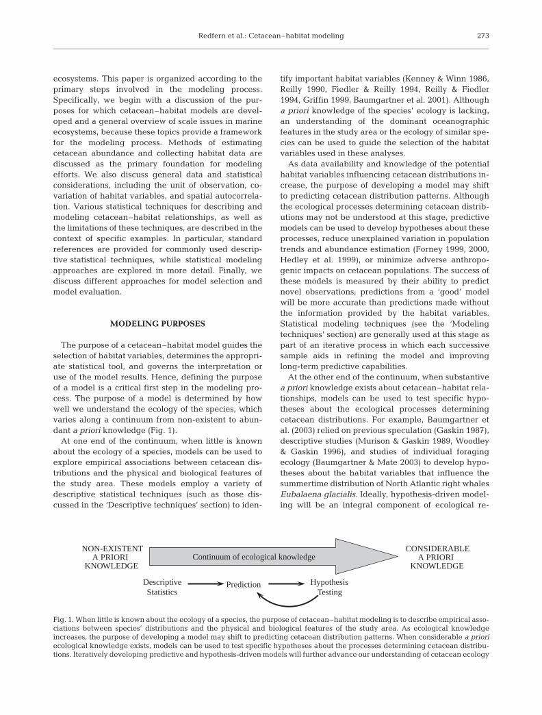
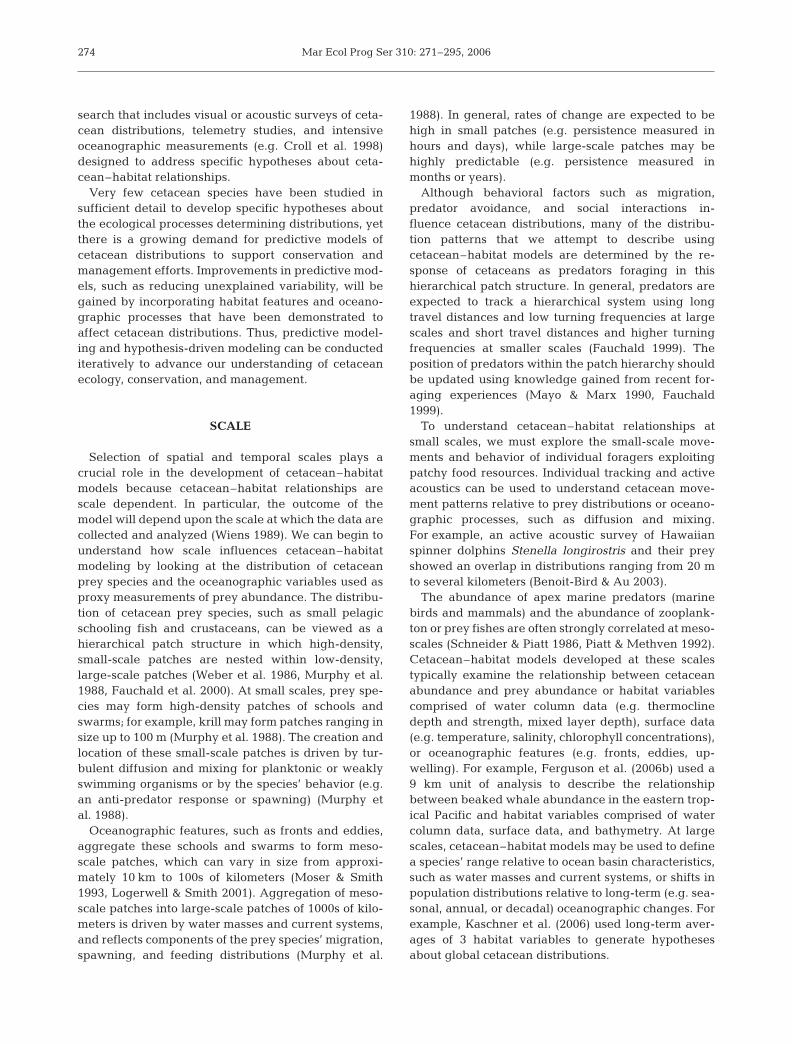
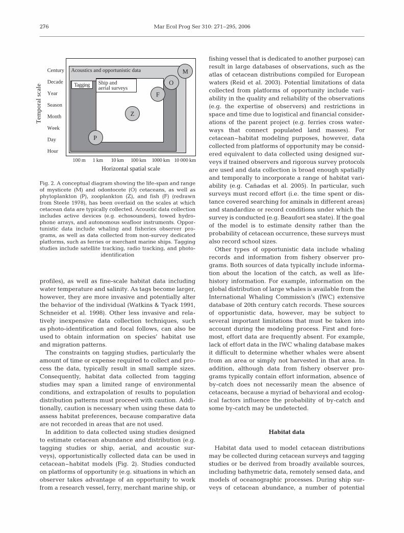
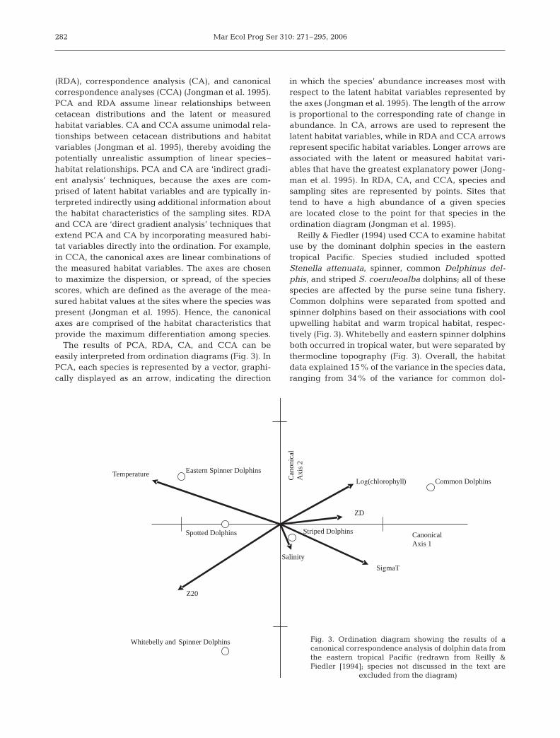
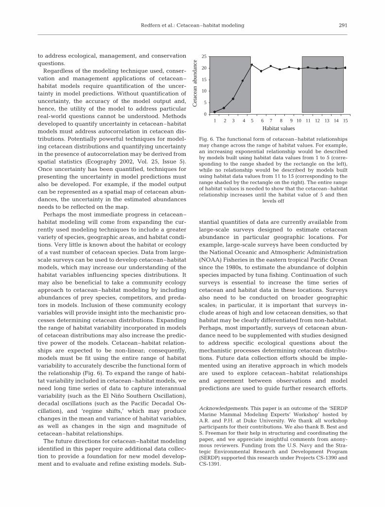


![Influence of ocean fronts on cetacean habitat selection ...cetus.ucsd.edu/Publications/Dissertations/CamachoMAS_2010.pdf · CapstoneFinal_DCamacho [Compatibility Mode] Author: Greg](https://static.documents.pub/doc/80x56/5f506fb2b76f66060919cbdf/influence-of-ocean-fronts-on-cetacean-habitat-selection-cetusucsdedupublicationsdissertationscamachomas2010pdf.jpg)

![Influence of ocean fronts on cetacean habitat selection ...cetus.ucsd.edu/Publications/Presentations/MAS... · CapstoneFinal_DCamacho [Compatibility Mode] Author: Greg Created Date:](https://static.documents.pub/doc/80x56/5f61ce1025554e090f0fee86/influence-of-ocean-fronts-on-cetacean-habitat-selection-cetusucsdedupublicationspresentationsmas.jpg)


