Technische Universität München Laboratory Experiments using Low Energy Electron Beams with some...

Technische Universität München

Laboratory Experiments using Low Energy Electron Beams with some Emphasis on

Water Vapor Quenching

A. Ulrich, T. Heindl, R. Krücken, A. Morozov, *J.Wieser

Technische Universität München, Physik Department E12*Coherent GmbH

Air Fluorescence WorkshopL‘Aquila, Italy, Feb. 2009


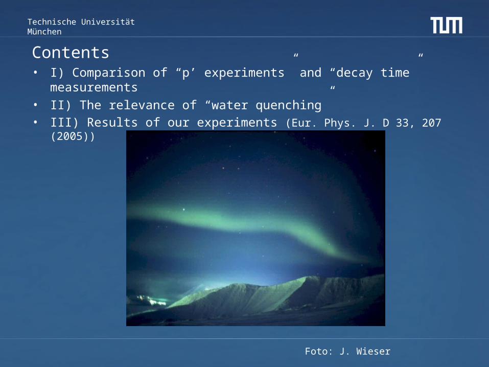
Contents• I) Comparison of “p’ experiments” and “decay time”

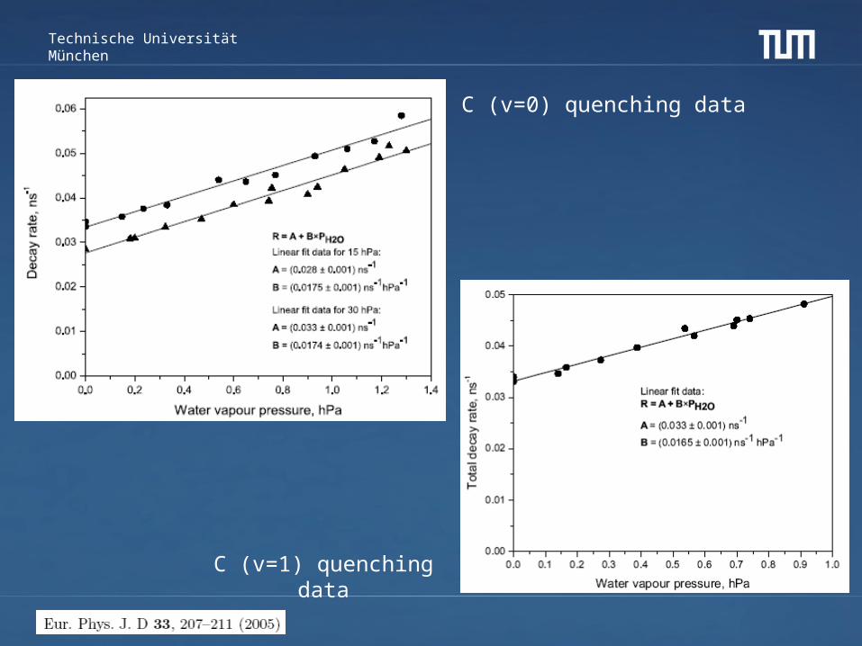
measurements• II) The relevance of “water quenching”• III) Results of our experiments (Eur. Phys. J. D 33, 207 (2005))

Foto: J. Wieser


Light Production by Particle Collisions

The elementary process of light production:

Collisional excitation of atoms or molecules and the

subsequent emission of photons:

Proj + X Proj‘ + hν

Electron or Ion (Proj)

Atom or molecule

Photon (hν)

Proj‘


The simplest case of data analysis:

radiativeTransitionro

Collisionally induced transitions

n*

Two types of measurements which should match! Measuring p’ or r0 and all Qq

?

'

,

''.

''

.,

,

..,.

.,,

.

*

**

*.,,

1

1

;:.

;;

1

1

;

;

q

qjiLight

qqtotaloptqqqq

qq

totalopt

qqjiLight

optjioptqqopt

pjioptjiLight

qqopt

p

qqoptdecaydecayprod

ijioptjiLight

p

pI

pnrnQforppDef

pn

r

nQI

rfrnQr

rrI

nQr

rn

nnQnrrrr

nrI


Method for Inducing Particle Collisions

E

Intensity vs. pressure

Pulsed excitation, time resolved measurement

Global light output vs. local light output

(Correction for geometry effects)

Detection Issues:


The p’ Method:

Data always have to be extrapolated to 0 pressure!

The geometry of the light emitting volume will always change!

There may be a background, scattered light etc.

For an example: See Thomas Heindl


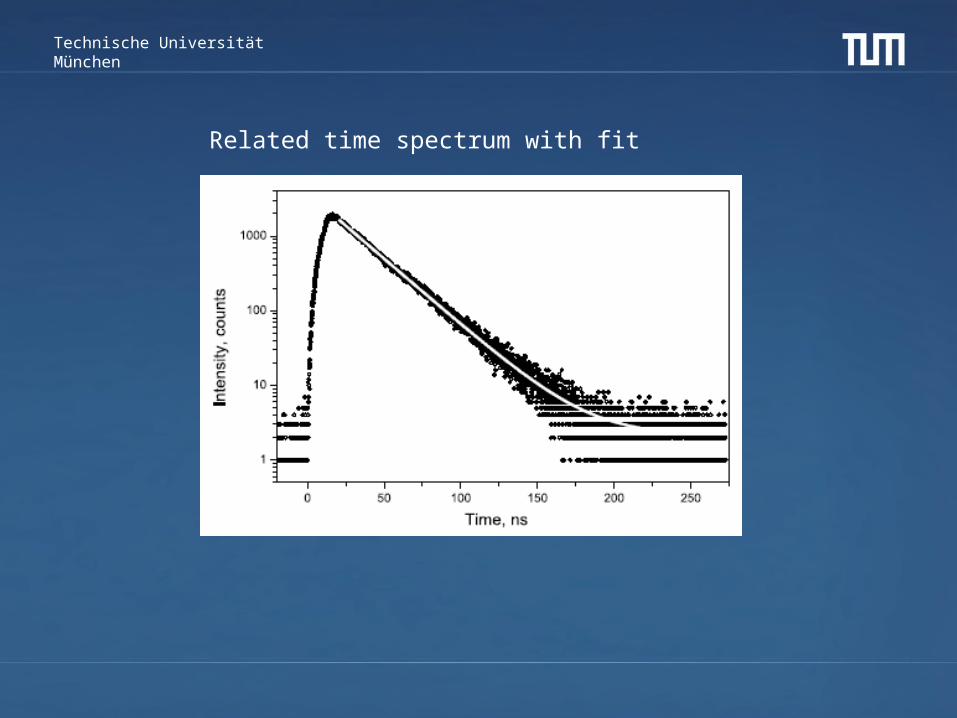
The Decay- Time Method:

The exponential decay has to be extracted from:

The time structure of the excitation pulse!

The background signal appearing at late times after the excitation!

Slowing down times of the projectiles may have to be considered!

The t – axis has to be well calibrated!

In case of ”TAC” spectra: “Clean” statistics


Tilo Waldenmaier et al.: Astro-ph Feb 2008

A. Morozov et al.: Euro Phys. J D 46, 51 (2008)


Intermediate summary:

• Both measuring techniques have their problems:

• Decay time measurements need short excitation pulses, a good dynamic range of the data, a reliable analysis and fitting procedure

• The p’ measurements have the problems of variation in the geometry of the light emitting volume with pressure

• Also: The “physics” connecting the two measurements may not be as simple as assumed!

• In practice this may cause a conceptual problem: Should the air shower experiments be analysed via tables of p’ values for all conditions found in the atmosphere or via calculation starting from N2 data? A combination of both techniques may be desireable but conceptually wrong.


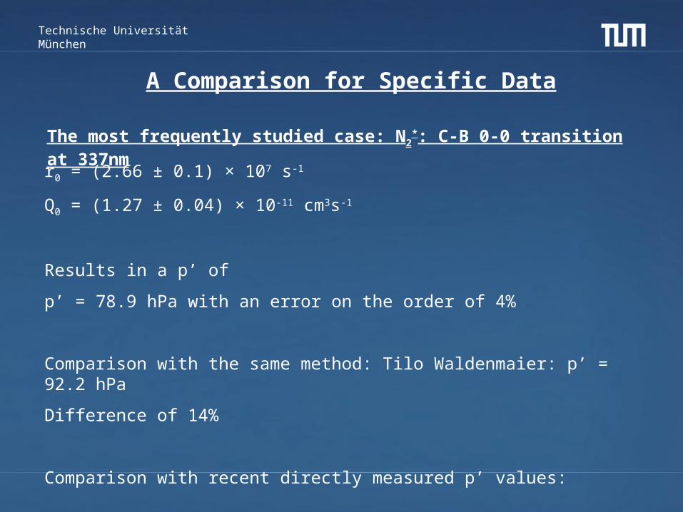
The most frequently studied case: N2*: C-B 0-0 transition at

337nmr0 = (2.66 ± 0.1) × 107 s-1

Q0 = (1.27 ± 0.04) × 10-11 cm3s-1

Results in a p’ of

p’ = 78.9 hPa with an error on the order of 4%

Comparison with the same method: Tilo Waldenmaier: p’ = 92.2 hPa

Difference of 14%

Comparison with recent directly measured p’ values:

A Comparison for Specific Data


Andreas Obermeier: Diplomarbeit page 45


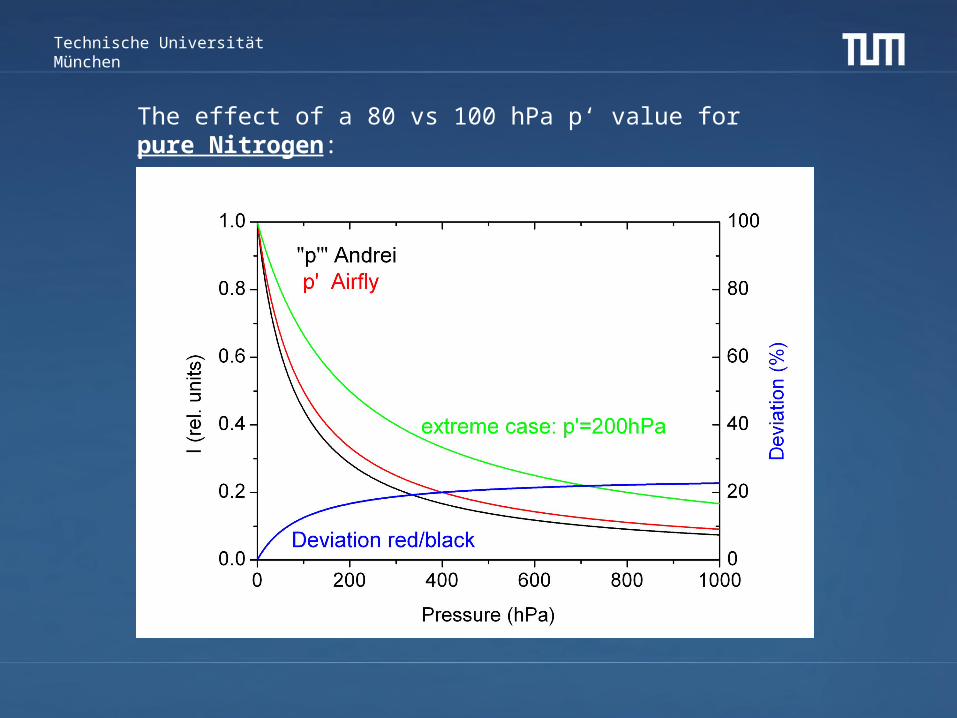
The effect of a 80 vs 100 hPa p‘ value for pure Nitrogen:


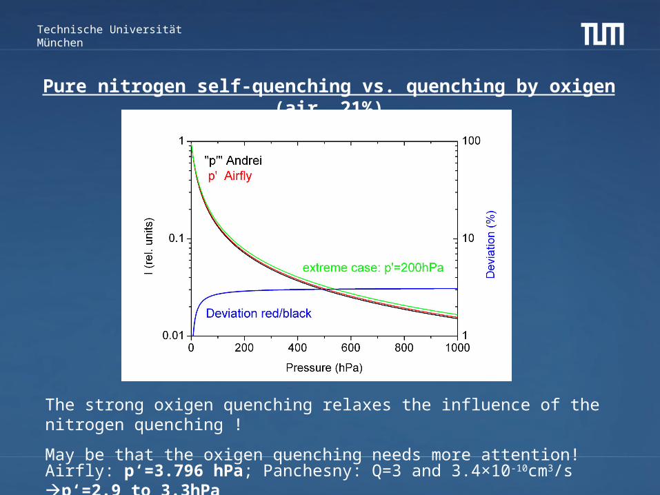
Pure nitrogen self-quenching vs. quenching by oxigen (air, 21%)

The strong oxigen quenching relaxes the influence of the nitrogen quenching !

May be that the oxigen quenching needs more attention!Airfly: p‘=3.796 hPa; Panchesny: Q=3 and 3.4×10-10cm3/s p‘=2.9 to 3.3hPa


The Issue of N2* Quenching by Water Vapor:

Available data (C, v=0):

AIRFLY: p’=1.28 hPa

Tilo Waldenmaier: p’=1.82 hPa Q=(5.43±0.12)×10-10 cm3/s

Andrei Morozov: p’=1.39 hPa Q=(7.1±0.7) ×10-

10 cm3/s

The difference between AIRFLY and Andrei Morozov is only about 8%

The data were recorded at up to 25 hPa and 1.4 hPa, respectively !


About water vapor in the atmosphere

Maximum amount of water:

3 to 30 g/m3 for –10 to 30 dec C


Result: The 0 and 4 km altitude cases of water content in air at 60% rel. humidity:

From 2.2 to 22 hPa partial pressure!


An overview over the “budged” of quenching data:

So far we have been working with quenching data – so the data are shown and compared in the “quenching world” and only for the C(v=0) level:

Optical decay rate: 2.66×107 1/s

N2* quenching by N2: Q=1.27×10-11 cm3/s

N2* quenching by O2: Q=30×10-11 cm3/s

N2* quenching by H2O: Q=71×10-11 cm3/s

Two scenarios:

Ground-level, 30 deg. C., 60% rel. hum., 1000 hPa total pressure

Max. Intensity effect due to water vapor: Iwet/Idry = 0.84; 16% effect

4km - level, -10 deg. C., 60% rel. hum., 600 hPa total pressure

Max. Intensity effect due to water vapor: Iwet/Idry = 0.86; 14% effectExample: I ~ 1/(1+(26N2 + 165O2 + 42H2O)/2.66)

Technische Universität MünchenExperiments using low energy electron beam excitation:


Aspects concerning water vapor measurements:• Nitrogen or air with a well defined water concentration is difficult to prepare

• Water vapor is adsorbed or released from the walls of the target cell

• Water vapor pressure is difficult to measure accurately

• UV light and the beam may dissociate water molecules

Some solutions:• Gold covered walls of the target cell

• Concentration measurement with a high precision capacitive manometer


Related time spectrum with fit


C (v=0) quenching data

C (v=1) quenching data


Future experiments that could be performed:

A) A p’ measurement with reduced geometry problems

e-guntarget cell

Ulbricht sphere

fiber opticssensitive USB spectrometer

p

B) Measurement of the quenching constant for O2 if it seems to be necessary ?

It would / will require a shorter electron beam pulse (Photocathode ?)

Expected results: Rel. Intensities of the bands, p’ values, absolute yield values


Thank you for your attention !

Date post:	28-Dec-2015
Category:	Documents
Upload:	coleen-young
View:	213 times
Download:	0 times

Technische Universität München Laboratory Experiments using Low Energy Electron Beams with some...

Documents