1

TECHNOLOGY DEVELOPMENT FOR EXOPLANET MISSONS

Technology Milestone White Paper

Enhanced direct Imaging exoplanet detection with astrometry

mass determination

February 8, 2016

Eduardo Bendek, P.I. Ruslan Belikov, Olivier Guyon,

Thomas Greene, and Eugene Pluzhnik JPL Doc: 1521447 National Aeronautics and Space Administration Ames Research Center Moffett Field, California

2

Signature page

Approvals: Eduardo Bendek, Principal Investigator Date NASA Ames Research Center/BAERI Nicholas Siegler, Technology Manager Date Exoplanet Exploration Program Douglas Hudgins, Program Scientist Date Exoplanet Exploration Program, NASA HQ

3

Table of Contents 1! Objective ....................................................................................................................... 4!2! Introduction ................................................................................................................... 4!

2.1! Background ............................................................................................................ 4!2.2! Combined astrometry and direct imaging .............................................................. 5!2.3! Perceived Impact .................................................................................................... 7!2.4! Relevance of work to element programs on the NRA ........................................... 9!2.5! Expected significance .......................................................................................... 10!

3! Milestone definition .................................................................................................... 11!4! Experiment description ............................................................................................... 12!

4.1! Modeling the diffractive pupil ............................................................................. 12!4.2! Astrometry laboratory limitations ........................................................................ 14!4.3! Laboratory status .................................................................................................. 15!4.4! Laboratory design ................................................................................................ 15!

4.4.1! The light source simulator ............................................................................ 15!4.4.2! Astrometry module design overview ............................................................ 15!

5! Data Measurement and analysis.................................................................................. 17!5.1! Data measurements .............................................................................................. 17!5.2! Data Reduction Algorithm ................................................................................... 18!5.3! Algorithm validation ............................................................................................ 21!5.4! Experiment error budget ...................................................................................... 22!5.5! Computation of the Metric ................................................................................... 23!

5.5.1! Definitions..................................................................................................... 23!5.5.2! Astrometry measurement .............................................................................. 25!5.5.3! Contrast calibration ....................................................................................... 27!

5.6! Milestone Demonstration Procedure .................................................................... 28!5.6.1! Astrometry milestone .................................................................................... 28!5.6.2! Combined imaging and astrometry milestone .............................................. 28!

6! Success Criteria ........................................................................................................... 28!6.1! The astrometry milestone success criteria ........................................................... 28!6.2! Direct imaging milestone success criteria ............................................................ 29!6.3! Success criteria conditions ................................................................................... 29!

7! Certification ................................................................................................................ 29!7.1! Milestone Certification Data Package ................................................................. 29!

8! Schedule and management .......................................................................................... 30!8.1! Plan description .................................................................................................... 30!8.2! Risk Assessment and mitigation plan .................................................................. 31!8.3! Management structure .......................................................................................... 31!

9! References ................................................................................................................... 33!

4

1 Objective This White Paper (WP) explains the purpose of the Milestones specified for the

Enhanced direct Imaging exoplanet detection with astrometry mass determination project, to be executed in support of NASA’s Exoplanet Exploration Program and the ROSES Technology Development for Exoplanet Missions (TDEM). This White Paper specifies the methodology for computing the milestone metrics, and establishes the success criteria against which the milestone will be evaluated. The first milestone is concerned with a demonstration of medium fidelity astrometry accuracy and the second milestone will demonstrate simultaneous medium fidelity astrometry and high-contrast imaging. 2 Introduction

TDEM Technology Milestones are intended to document progress in the development of key technologies for a space-based mission that would detect and characterize exoplanets, such as EXO-C (Stapelfeldt et al. 2015), AFTA-C or smaller (to be defined) Explorer-class mission, thereby gauging the mission concept’s readiness to proceed from pre-Phase A to Phase A.

2.1 Background Stellar astrometry is one of the most promising exoplanet detection and

characterization techniques, allowing the determination of planetary mass and orbit, solving the system inclination ambiguity, and determining the coplanarity of planetary systems (Levine et al. 2009; Papaloizou & Terquem 2001). However, only a few planets have been detected using stellar astrometry because the signal of most of the habitable exoplanets around nearby stars (<10 pc) causes a sub-microarcsecond (µas) signal on their host star. Therefore, they are undetectable for today’s most advanced instrumentation. For example, an Earth-like astrometric signal ranges from 1µas for Sun-like stars at 3pc to 0.3µas at 10pc distance. For detections with Signal to Noise Ratio (SNR) equal to 5, the final astrometry accuracy must be in the range of 0.2 to 0.06µas, which could be obtained with 25 observations per target visit, each with 0.3µas accuracy per observation if the noise is uncorrelated. This strategy has been considered for other astrometry missions. For the purpose of this White Paper the stellar astrometry accuracy value are specified per observation.

High-precision stellar astrometry enhances other exoplanet detection techniques, such as direct imaging. In fact, detailed exoplanet characterization requires both direct imaging and stellar astrometric measurements; these combined measurements offer greater detection sensitivity and reliability than possible with separate missions (Lunine et al. 2008; Shao et al. 2010; Guyon et al. 2013a).

High-precision stellar astrometry can complement high-performance coronagraphy measurements allowing improved detection and full characterization (including masses) of exoplanets. Both masses and spectra are needed to truly understand the surface gravity, thermal profile, and chemical composition of planets. This is especially important for planets that could populate the Habitable Zone (HZ). Planets within the HZ exhibit a longer period and larger angular separations compared to hot planets commonly detected with (Radial Velocity) RV and transit techniques. For these

5

reasons, planets located in the HZ are dimmer than their hotter counterparts, increasing their contrast ratio, placing them in the lower right corner of the plot of Figure 1. This area of higher angular separation and high contrast corresponds to the operational regime of space telescopes. This supports the claim that stellar astrometry is well suited to complement High-Contrast imaging from space. In contrast, planets with high RV have low separation and low contrast making them ideal to observe with large telescopes from the ground.

Moreover, stellar astrometry can probe planetary regions difficult to reach using RV and transit measurements. RV’s sensitivity reduction to planets at larger Semi-Major Axis (SMA) limits its ability to detect habitable planets. In contrast, the astrometric signal increases with SMA, therefore facilitating habitable planet detection, mass measurement, system inclination and false positive verification. Planets that induce a high-astrometric signal require high contrast to be observed. These are also located at a large angular separation from the star, making them ideal to observe from space.

As a result of the efficiency that combined direct-imaging and astrometry offer this approach has been proposed for two mission concepts, ExO (Blackwood et al. 2013) and EXACT (Guyon et al. 2013b). In the case of the former, a 2.4m space telescope could be equipped with a high-performance coronagraph and an astrometric camera that would be able to obtain sub-µas astrometry for a mv = 3.7 Sun analogous star at a distance of 6 parsecs.

2.2 Combined astrometry and direct imaging The main limiting factor in sparse-field astrometry, besides photon noise, is the

non-systematic dynamic distortions that arise from perturbations in the optical train (Benedict et al. 1994; Guyon et al. 2012a; Trippe et al. 2010). To improve the astrometric measurements, it is necessary to increase the number of background stars by using a wide-field camera. However, as the Field of View (FoV) increases, distortion dominates the error budget; hence, the challenge is to achieve long-term distortion stability on a wide-field camera.

Even space optics suffer from dynamic distortions in the optical system at the sub-µas level. To overcome this limitation, a concept has been proposed (Guyon et al.

Figure 1. The astrometric signal versus contrast of

hypothetical exo-earths1-Earth-mass planet orbiting in the middle of the HZ for stars within 10pc is shown in this plot. The circle size represents angular separation, and its color the RV signal in [m/s], showing that astrometric signal is larger for planets with high angular separation and high

contrast (lower right), which is the space telescopes regime.

6

2012a) which uses a Diffractive Pupil (DP) to generate precise fiducial features in the image plane, which appear as radial streaks or spikes. These diffractive features can calibrate dynamic or relative distortions because they are imaged by the same optical system. Therefore, their positions also change with distortions, thus serving as a reference for calibration. Researchers have proposed using a diffractive grid for narrow-field astrometry applications (Marois et al. 2006; Sivaramakrishnan & Oppenheimer 2006). Here we propose the application of the DP concept to wide-field cameras.

In order to create diffractive fiducial features in the image plane, a periodic array of small dots is imprinted on the primary mirror of the telescope. These dots create diffraction and generate a new array of dots with inverse spatial frequency, as predicted by the Fraunhofer far-field diffraction. These dots are smeared radially in broadband light forming “diffraction spikes”.

The astrometric signal of the central star is then measured by comparing the position of the diffraction spikes to the background stars instead of comparing directly to the host star Point Spread Function (PSF). Figure 2, top row, shows how the astrometric signal of the host star will move the spikes with respect to the background star field. In the presence of dynamic distortions between measurements, as shown in the second row of Figure 2, the PSF location of a star is biased by the distortions. However, if the distance is measured to the spike, this effect is calibrated.

To asses the capabilities of the technique we consider a baseline telescope design that has a 1.4m aperture with dots covering 1% of the primary mirror area, and with a 0.3 deg2 Field of View (FoV) camera with 44 mas pixels observing in visible light. We assume that this system is observing a Sun-like star at 6pc (mV = 3.7).

Figure 3: EXACT Concept using a coronagraph and DP for high precision astrometry in a single mission. A mirror at an

intermediate focal plane directs the central field to the coronagraph and reflects the wider field to the astrometric

camera.

Figure 2. Astrometry calibration algorithm

using the diffractive spikes. On the top row two measurements or epochs are shown for a perfect system. An astrometric signal creates a uniform

differential motion of the pixels and the reference stars. In the lower row a system that is

affected by distortions causes errors in the astrometric measurement, which can be

calibrated using the diffractive spikes as a reference.

7

By applying a DP to calibrate dynamic distortions and rolling the telescope that can improve sensitivity by averaging down detector effects, it is possible to achieve 0.2 µas astrometric accuracy (Guyon et al, 2012a).

This technique is compatible with a direct imaging mission; since the astrometric signal of the host star is measured with respect to the spikes and not to the star PSF. The implementation of a combined mission is based on a wide-field telescope that has two instruments: a wide-field astrometry camera that images the background stars and the diffractions spikes, and a coronagraph that images a narrow field around the host star where the planet is expected. The narrow FoV is separated from the optical train with a pick-off mirror. This combined architecture, shown in Figure 3, enables both detection techniques simultaneously. This concept works for a wide range of mission sizes, but the ultimate accuracy strongly depends on the aperture size and the FoV of the telescope.

Notes about the impact of the DP on the telescope performance:

The telescope DP must be placed on the first optical surface because it only calibrates optical distortions AFTER the DP location. We have been assuming that it would need to be placed at the primary mirrors in this White Paper. We note that if other means to calibrate distortions were available for the primary mirror, the DP could be placed downstream of the primary mirror.

According to models, the light contamination due to the diffraction spikes is expected to be negligible compared to other errors in the system due to the telescope spider or segmentation (if present). The baseline design DP, which considers covering 1% of mirror area with dots, creates less diffracted light than a typical telescope spider that covers approximately 5% of the primary mirror.

From the coronagraph point of view the energy diffracted by the DP lies outside the FoV of the coronagraph because the DP has only high spatial frequencies. For the wide-field camera, the additional background due to diffracted light by the dots would not significantly affect the performance of the telescope for general astrophysics applications. For the baseline design the additional light introduced by the dots on the primary mirror is less than 1% of the zodiacal background when a mV=3.7 star is observed. Therefore, the DP would have a limited impact on the wide-field camera and trade of the dots size will be required to find the optimal design that balances astrometric accuracy and background contamination.

2.3 Perceived Impact Several astrometry (Unwin 2005; Shao et al. 2009; Malbet et al. 2011) and direct

imaging concepts (Levine et al. 2009; Guyon et al. 2010; Trauger et al. 2010; Clampin et al. 2006) have been proposed for identification and characterization of nearby exoplanets, demonstrating the technical feasibility of either measurement approach. The efficiency and sensitivity of exoplanet-detection missions can be augmented by adding astrometric measurements to the coronagraphic observations, which will confirm direct imaging detections and help to constrain the orbital parameters and masses of the exoplanets. In addition, astrometric measurements offer several other advantages, including revealing planets inside the Inner Working Angle (IWA) of the imaging system, helping to identify targets for a spectroscopic mission, reducing the false positive rate, and mitigating the 1 year period blind spot that an astrometry-only mission would have. Adding

8

coronagraphic images to the astrometric data reduces the standard deviation on orbital parameters by approximately a factor of 10, and over a 2-year combined mission the masses and Semi-Major Axes (SMA) estimates are better than a 4-year only astrometry mission, as shown by a simulation in Figure 4 (Guyon et al. 2013a).

Figure 4. Monte carlo simulation of best parameters solution of a three-planet system showing the

benefit of using astrometry and direct imaging data to constrain system orbits and masses. (Measurements shown in bottom left) after astrometry, (measurement shown in top left, gray circle

shows coronagraph IWA within which no measurement is available) after coronagraphy.

9

The impact of this work is the demonstration and performance characterization of combined astrometric and direct imaging measurements in the laboratory. The proposed work will serve as a testbed to assess the feasibility of implementing astrometry on exoplanets missions such as EXO-C, EXO-S (if its FoV is enlarged) and other future flagship missions

The combined direct-imaging and astrometry laboratory will mitigate risks associated with a real mission by using the same optical layout and technologies scaled down in size, therefore testing the concepts, validating the error budgets (See section 5) and exploring potential sources of incompatibility of both techniques that have not been identified when they are tested separately. Finally, this concept will advance the relevant technology in the following ways: • Advance the DP concept from TRL3 to late TRL4. This is important to propose and

evaluate any future astrometry exoplanet mission, as well as general astrophysics missions that require enhanced astrometry.

• Advancing further the technology to manufacture the DP over curved mirror surfaces. • Development and laboratory validation of data reduction algorithm(s) to calibrate

astrometric distortions with the DP concept. • Demonstrate DP compatibility with high contrast imaging at the 5x107 contrast level

at 1.6 λ/D. We will do so by achieving 5x107 RAW contrast between 1.6 and 6λ/D behind a DP showing that the light diffracted does not cause light contamination of coronagraph FoV that might diminish it performance.

• Demonstrate 2.4x10-4 λ/D astrometric accuracy in the laboratory per axis, which is equivalent to 5 µas on a 2.4-meter class space telescope per axis, without affecting the coronagraphy performance.

• Model and measure the diffractive spike flux over the wide imaging field to provide the information necessary for future investigations to assess the impact on astrophysics science programs that do not require bright stars in the FoV.

From long-term strategic perspective this proposal aims to recover NASA’s leadership in the astrometry field after the cancellation of The Space Interferometry Mission (SIM) and its variants.

2.4 Relevance of work to element programs on the NRA Combined direct imaging and astrometry determines exoplanetary orbital parameters and masses faster than using direct imaging only, reducing the cadence necessary to characterize exoplanetary systems and therefore increasing the number of systems that may be studied in a mission lifetime. Also, astrometry is particularly important for differentiating between terrestrial and mini-Neptune planets as well as between Neptune mass and giant planets (Cahoy et al. 2010). In addition, a key strength of the simultaneous coronagraphy and astrometry measurements is the mitigation of confusion that would occur in a purely direct imaging mission. Planetary systems are likely to contain multiple planets and circumstellar dust. Inner planets in habitable zones will probably be visible in a subset of the coronagraph observations. Astrometric measurements will help identify planets in multiple systems and will solve the ambiguity between nearly mass-less exozodiacal cloud features and exoplanets.

10

Adding astrometric capabilities to a starlight suppression system complies with the NRA request “solicits investigations that will undertake focused development of technologies that feed into the key starlight suppression techniques for direct detection of exoplanets”. Furthermore, the NRA emphasizes the development of technologies for Earth-like planet detection in preparation for a down select in 2015 and readiness for a flagship mission in the 2020 decade. This proposal will also help develop instrumentation and missions that address the NASA strategic call for “progress in understanding how individual stars form and how those processes ultimately affect the formation of planetary systems” (NASA Strategic Plan - 3.D.3), and “creating a census of extra-solar planets and measuring their properties” (NASA Strategic Plan - 3.D.4). This work also directly builds on an already demonstrated successful investment into the development of high precision astrometry using a DP by NASA, Guyon APRA’10 (Astrometry laboratory demonstration) Additionally, this proposal continues the NPP work completed by the PI of this TDEM. This NPP project developed a basic low-cost combined, astrometry and direct imaging capabilities at the ACE laboratory. NASA has invested significant resources in coronagraphy, and continues to do so. Adding astrometry will boost the efficiency and reliability of coronagraph measurements; it also reduces confusion and has the potential to identify planets more rapidly than direct imaging and measuring their orbits, which will optimize use of telescope time. This ongoing effort, together with other proposals (Belikov APRA’13), directly builds on an already demonstrated track of successful investments into the development of the Phase Induced Amplitude Apodization (PIAA) and other coronagraph-related technologies by NASA. From a strategic point of view this proposal extends the Ames Coronagraph Experiment (ACE) laboratory capabilities to the astrometry area and therefore offer to NASA and the community a unique facility to advance exoplanet detection technologies. !2.5 Expected significance

This proposal will demonstrate the efficient combination of direct imaging and stellar astrometry validating the scientific and cost advantages of the approach. Having an integrated laboratory will characterize performance and demonstrate the feasibility of this technique. Representative examples of missions that would benefit from having the astrometry capability are ExO (Blackwood et al., 2013), EXACT (Guyon et al., 2013b), EXO-C and EXO-S and even AFTA/WFIRST. In general, this work will support NASA Strategic plans by developing a unique facility to validate any future mission concept or flagship exoplanet mission, such as the Habitable-Exoplanet Imaging Mission that would combine high contrast imaging and astrometry. This work will advance the DP ability to calibrate field distortions, which can benefit other astrometry related general astrophysics science cases that can be performed using a wide-field astrometry instrument, In particular this project will: • Demonstrate in the laboratory that direct imaging techniques can be augmented by

adding an astrometric capability. This will enable a single exoplanet flagship mission to perform the task that was originally expected to require two separate missions (high-precision astrometry and direct imaging), resulting in substantial advantages in cost and schedule.

• Greatly enhance the scientific return of any coronagraph mission by reducing

11

confusion issues due to exozodiacal light structures and multiple planets. In fact multiple planet systems can be characterized with only 6 observation epochs (Guyon et al, 2013a).

• Understand the technical implementation challenges of combining coronagraphic direct imaging and DP astrometry in greater depth to generate a detailed error budget needed for a future high fidelity demonstration and mission concept planning.

• Create and validate experimentally astrometry performance models that will predict the system astrometric accuracy as a function of telescope size, FoV and DP design. The model will also assess the light contamination produced by the DP over the full FoV, allowing the community to perform trade studies of the DP for general astrophysics science cases.

• Explore the potential benefits of using the astrometric signal to accurately and independently measure spacecraft pointing and characterize flexing of the spacecraft bus and optical components by means of tomographic reconstruction using the motion of the diffractive spikes (Guyon 2012a).

• Advance mirror coating technology that allows applying high performance coatings with special shapes needed for astrometry and other advanced optical calibrations.

3 Milestone definition

Completion of these milestones is to be documented in a report by the Principal Investigator and reviewed by the Exoplanet Exploration Program. The milestones read as follows:

Milestone #1 definition: Broadband medium fidelity imaging astrometry demonstration Demonstrate 2.4x10-4 λ/D astrometric accuracy per axis performing a null result test. The laboratory work will be carried out in broadband spectrum covering wavelengths from 450 to 650nm using an aperture pupil (D) equal or larger than 16mm.

The “angular separations” are defined in terms of the source wavelength λ, and the diameter D of the aperture on the DP, which is the pupil-defining element of the imaging astrometry camera. For this milestone, a DP simulates the telescope primary and pupil and it will illuminated by an array of broadband point sources forming f/25 to f/50 beams when they reach the pupil.

Milestone #2 definition: Broadband medium fidelity simultaneous imaging astrometry and high-contrast imaging Demonstration of milestone #1, and performing high-contrast imaging achieving 5x107 raw contrast between 1.6 and 6λ/D by a single instrument, which shares the optical path, from the source to the coronagraphic and astrometry FoV separation. The ability of achieving 5x107 raw contrast will be considered as proof of no contamination of the IWA.

At the end of this TDEM the TRL of this technique should be late 4. In addition to the milestones we will produce a detailed error budget that will allow us to validate our simulations with experimental data, and create performance models that can predict the

12

system astrometry accuracy as a function of telescope aperture and FoV. We will also compute the amount of light diffracted by the DP over the wide-field informing missions design and planning. Table 1: Astrometric accuracy for this proposal and TRLs.

Project Astrometric accuracy [λ/D] StartTRL EndTRL First lab demonstration 3.42x10-3 1 3 This TDEM Milestone* 2.40x10-4 3 4 *The lab test for these cases uses D=0.016m.

4 Experiment description

Astrometric measurement from wide-field images is fundamentally limited, in a perfect system, by photon noise and sampling effects. These fundamental limits are, however, not the focus of this TDEM, which is aimed at providing a solution to the three main practical challenges to performing precision imaging astrometry of a bright star using numerous faint field stars as astrometric reference.

1. Dynamical range. There is a large brightness difference between the central target star and the surrounding field stars, making it difficult for a detector to properly image both.

2. Distortions. Slight deformations of the optical surfaces, or the detector focal plane array, introduce astrometric errors. These errors tend to grow larger in amplitude as the field of view (FOV) is increased.

3. Detector defects. The geometry and response of pixels are not known to sufficient accuracy to allow high-precision astrometry from a single wide-field image.

The diffractive pupil astrometry optical principle solves the first two challenges by creating in the wide-field focal plane image diffraction spikes. These spikes are of comparable surface brightness as the field stars (solves the dynamical range challenge) and experience the same distortions as the field stars used as the astrometric reference (solves the distortion challenge).

4.1 Modeling the diffractive pupil To calibrate time-varying distortions, the spike spacing on the image plane should

provide at least a Nyquist sampling of the optical system distortion spatial frequencies. This requirement drives the periodicity and geometry of the dot pattern in the pupil. The dot size controls the relative brightness between the central star and the spikes, creating an appropriate set of references for astrometry (Bendek et al. 2013b). Under monochromatic illumination, the DP creates an inverse spatial frequency array of diffractive spots on the image plane. The pattern for this experiment can be represented as a pupil of diameter D, which has a hexagonal grid of dots of diameter d, with a side of length a, as shown in Figure 5.

The hexagonal pattern can be modeled as a replication of pairs of delta functions over the pupil plane and can be mathematically represented as:

13

!"#, %& ' (*+,- .!"#$

, %"√#$

/ ∗ 122 3!"!"

#

, %"√!"

#

4 ∗ 22 .!"$/5, (1)

where the comb function is a two-dimensional array of delta functions, !!

represents a pair of delta functions, and A represents the scaling factors required to maintain the normalization of delta functions. The x and y axis have been multiplied by the aperture D to normalize the result to the aperture size. At the image plane the Fourier transform of this grid is obtained as,

6 ' 7'7(8!"#, %&9 ' *+,- .#$":, √#$

";/ <cos.#)$

*":, √#)$

*";/ *+@ .)$

":/A, (2)

where " and # represents the transform variables and axes in the image plane. On the image plane we obtain a bi-dimensional comb function with spacing D/3a along the " axis. This grid is modulated by two cosine functions. The first cosine is bi-dimensional and has a period of 4D/3a along the " axis, creating zeros at D/3a and D/a reducing the special frequency of the comb by half allowing deltas only at,

Figure 5. On the left, an image of the hexagonal arrangements of dots placed on the pupil is shown. Here, the side of the hexagon is defined as a, so the hexagon width is 2a wide. The “X” signs in the figure represent the periodic structure of the grid, and the “+” signs denote the center of each double delta function. On the right, the resulting image and spot spacing is shown. The dashed lines represent zeros of the cosine modulation that

eliminates the spot at D/3a.

" $ !

"

#

$, (3)

and at integer multiples of this value. Using the same rationale for the # axis, we obtain delta functions at,

# $ !√"

"

#

$. (4)

Similarly, the deltas are replicated at integer multiples of this value. The spot

brightness is modulated by the second cosine on eq. 2, which has a period of 2D/a but

14

does not change the spatial frequency of the grid because it does not have zeros matching the comb period.

4.2 Astrometry laboratory limitations Astrometry is based on measuring the relative change in position between

background or reference stars with respect to a target star. The fundamental limits of imaging stellar astrometry are twofold: From the astrophysics point of view, motion of the background stars can be caused by companions such as dwarf stars or planets. Also, star spots can modify the star centroid, but this error is expected to be less than 0.1µas for sun-like stars (Makarov et al. 2009). If we assume that these errors are random processes where the noise and the signal are uncorrelated, the error averages down as the number of stars in the FoV increases. From the instrumental point of view, the ultimate precision that astrometry can achieve is constrained by the photon noise, which limits the 2D centroiding accuracy of a single star to (Guyon et al. 2012):

!!" "#"# ! √!%

&'(!"

"#"#" (5)

The photon noise limit assumes monochromatic light and infinite sampling. The effect of broadband light and detector discretization due to finite pixel size increases this limit as the bandwidth increases and sampling decreases (Guyon et al. 2012). When real detectors are considered, Read Out Noise (RON) and Dark Current (DC) play a significant role in limiting the centroiding accuracy as well as the technique used to obtain the centroid.

For this experiment we chose to obtain centroiding positions using the Center of Gravity (CoG) algorithm, which simply averages the positions of the PSF pixels weighted by their intensity,

$%)*+ !∑ -#$%& .'!(∑ .'!(#$%&

, (6)

where $%)*+ is the PSF centroid in the x axis, &-!/ is the intensity of a pixel located at coordinates (x,y), and N is the number of pixels in the region of interest. The precision of the CoG algorithm is affected by the stars’ PSF aberrations and their Signal to Noise Ratio (SNR). A wide range of techniques exists to improve the performance of this algorithm, such as PSF fitting, deconvolution, and matched filters. However, in this paper we focus on demonstrating the ability of the diffractive pupil to calibrate distortions, for which we used a CoG algorithm. The effect of photon noise and RON on the centroiding accuracy of this technique has been previously discussed in the literature (Rousset 1999; Thomas et al. 2006) and is expressed as,

!- ! '!-!(01! # !-!(2!) , (7)

where !- is the centroid standard deviation, !-!(01! is the photon noise variance, and !-!(2! is the RON variance and

!-!(2! !(*)(+

,

&!(!") , (8)

and,

15

!-!(01! !(*)

345!(!") , (9)

where (01! is the average numbers of photons per spot per frame, or Region of Interest (ROI), (2! is the gaussian RON noise variance, (6! is the total # of pixels used in the calculation, and (7 is the FWHM of the stars in pixels.

4.3 Laboratory status Two astrometry experiments have been built successfully. The first one was the

development of a diffractive pupil astrometry demonstrator at University of Arizona funded by a NASA grant awarded to Olivier Guyon APRA’10 (Astrometry laboratory demonstration) and executed by Eduardo Bendek as part of his Ph.D. program.

Additionally, Dr. Bendek was a awarded with a NASA Postdoctoral Program fellowship that allowed him to develop a basic, low-cost combined, astrometry and direct imaging capabilities at the ACE laboratory to perform initial validation of the concept. Currently, this testbed is being re-designed and upgraded with funds of this TDEM grant.

4.4 Laboratory design

4.4.1 The light source simulator The laboratory design

considers using a common light source for the coronagraph and astrometry camera, simulating a star field with a brighter central target star in the center. To simulate the star field, a 100µm thick tungsten 1” diameter disc with a grid of 20x20 laser drilled 5µm holes is used. The holes, which are equivalent to point sources for the astrometry camera resolution, simulate background stars. On the back of the central hole, a 3mm diameter achromatic lens is glued precisely to place its focus on the center of the 5µm hole, creating a host star ~104

brighter than the background stars.

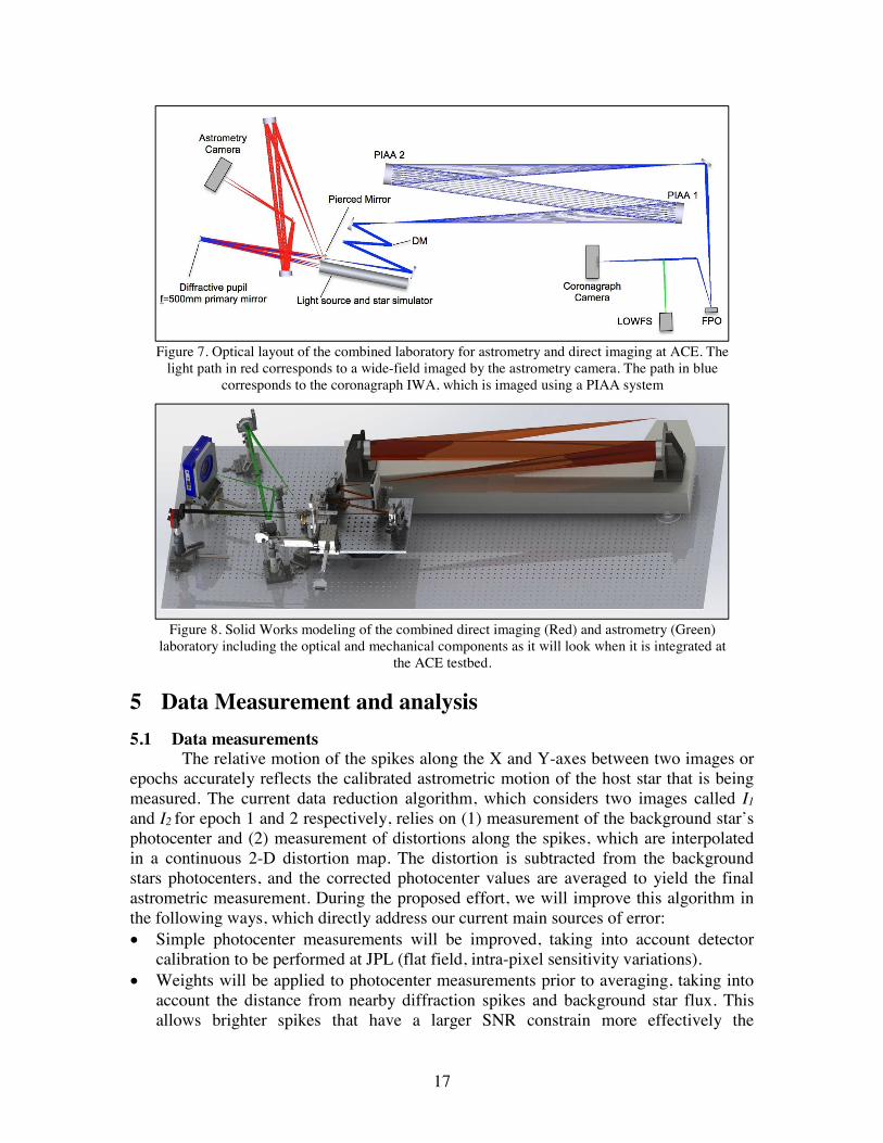
4.4.2 Astrometry module design overview A primary DP mirror, shown in figure 7, collects the light emitted from the star

simulator. This mirror is spherical and has a focal length of 500mm. Its aperture is 16mm to limit the spherical aberration. This mirror will also be coated with chrome or aluminum, and microscopic 10µm dots will be placed on a hexagonal arrangement where 120µm pitch creating first order radial spikes from 66.8 to 117 λ/D for 450 to 650nm spectrum as shown in Fig. 6 and summarized in Table 3. The DP mirror also acts as the stop and pupil for the astrometry camera and refocuses the diverging light from the star simulator in an intermediate focal plane.

Table 2: Astrometry experiment design parameters Optical design parameters Angular Focal plane Central wavelength 550nm N/A Broadband 200nm N/A Aperture D 0.016 N/A Sampling factor 2 N/A Pixels/(L/D) 4px 29.6µm Pixel size [um] 0.25λ/D 7.4µm Detector size [px] 3248px 24.0 mm HFoV [L/D] 406 λ/D 12.0 mm

16

Figure 6. Schematic showing expected location of the monochromatic (632nm) and broadband

(450-650nm) diffractive features is shown on the left image. The right image shows the diffractive pattern for the respective bands. The coronagraph field looks elliptical due to tilt of the pierced

mirror.

Before the intermediate focal plane a pierced mirror with an aperture in the center is placed to separate the wide field objects (shown in red) reflecting their light to a pair of off-axis parabolas and a fold mirror which creates a wide field image on the astrometry camera. The airy radius is 32µm and the image is diffraction limited and unvignetted over a field of 0.49 square degrees. The hole of the pierced mirror allows a coronagraphic FoV radius of 30λ/D, that contains the central star. The next element encountered is the BMC Kilo Deformable Mirror (DM) that has 1024 actuators. The DM is in a pupil plane allowing correcting any wavefront errors induced by the spherical DP mirror. Downstream the DM there is a PIAA based SSS that has other elements of the ACE baseline design, as shown in figure 7. Table 3: Diffractive pupil design

Coronagraph field [arcsec]

Hexagon size a

Dot Size 1st order location @ 632 nm

Spike width (450-650nm)

Angular location 30 λ/D 120µm 10µm 89 λ/D 66.8 - 117 λ/D Focal plane 0.5 mm NA NA 2.63mm 1.98 - 3.46mm

The design architecture is identical to the design proposed for combined space

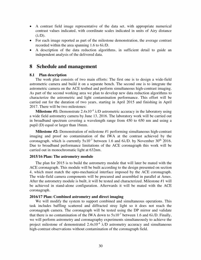
missions and will allow high contrast imaging and astrometry on the same test bed. The proposed design has been modeled in detail including optical, and mechanical component selection and geometrical compatibility with the ACE coronograph. Figure 8, shows a render of the complete opto-mechanical system model integrated at the ACE test bed.

17

Figure 7. Optical layout of the combined laboratory for astrometry and direct imaging at ACE. The

light path in red corresponds to a wide-field imaged by the astrometry camera. The path in blue corresponds to the coronagraph IWA, which is imaged using a PIAA system

Figure 8. Solid Works modeling of the combined direct imaging (Red) and astrometry (Green)

laboratory including the optical and mechanical components as it will look when it is integrated at the ACE testbed.

5 Data Measurement and analysis 5.1 Data measurements

The relative motion of the spikes along the X and Y-axes between two images or epochs accurately reflects the calibrated astrometric motion of the host star that is being measured. The current data reduction algorithm, which considers two images called I1 and I2 for epoch 1 and 2 respectively, relies on (1) measurement of the background star’s photocenter and (2) measurement of distortions along the spikes, which are interpolated in a continuous 2-D distortion map. The distortion is subtracted from the background stars photocenters, and the corrected photocenter values are averaged to yield the final astrometric measurement. During the proposed effort, we will improve this algorithm in the following ways, which directly address our current main sources of error: • Simple photocenter measurements will be improved, taking into account detector

calibration to be performed at JPL (flat field, intra-pixel sensitivity variations). • Weights will be applied to photocenter measurements prior to averaging, taking into

account the distance from nearby diffraction spikes and background star flux. This allows brighter spikes that have a larger SNR constrain more effectively the

18

interpolation process. • Astrometric measurements (corrected photocenters) will be marginalized against

modal distortion variations identified between measurements. The outcome of the data processing effort is a model that will predict the system

performance as a function of telescope size, FoV and DP design and geometry that will be validated experimentally. This model will also assess the impact of the DP in the wide field.

5.2 Data Reduction Algorithm The data reduction algorithm is based on the angular component of the spikes

position because the radial smearing of the diffractive features that create the spikes prevent accurate radial measurements. We only use the spike’s angular position change that is accurate; nevertheless, the Cartesian X-Y astrometric vector can be obtained by projecting multiple angular displacements into X-Y coordinates.

The algorithm starts by taking a reference image, Iref, as the sum of I1 and I2, and a difference image, Idiff. The next step in the data reduction process is to calculate the angular derivative, which provides a ratio on each pixel to convert the differential image Idiff pixel intensity into angular displacement.

To obtain the angular derivative, we first need to compute the Cartesian unitary derivatives of the reference image by taking Iref and subtracting from it by a 1 pixel shifted version of itself, first with respect to X and afterwards to Y. Then the Cartesian derivative terms are used to compute the angular derivative,

8.*-.89 ! $) 8.*-.

8- # $ 8.*-.8/ (10)

Then, the angular displacement is computed by dividing, pixel-to-pixel, the difference image, Idiff, with the angular derivative, given by eq. (11):

*:;60 !./$..01*-.

02

(11)

At this step the noise problem arises because the distortions to be measured are in the range of 10-2 to 10-5 pixels. However, in all other locations of the image where there are no spikes the noise level is orders of magnitude higher. To solve this problem, the SNR of the angular distortion measurement needs to be computed for every pixel. The signal is the value of the angular derivative and the noise is computed as the root sum square of the RON plus the photon noise,

+(, !

01*-.

02

(*;6< . (12)

The angular distortion image is multiplied with the SNR squared, amplifying the values along the spikes and minimizing them on the background,

*:;60"=(> ! *:;60+(,!. (13)

The image containing the angular distortion is noisy especially along the spikes. A binned version is created to reduce the noise level and the computational power required to process them. This process does not discard useful information because the

19

spikes remain resolved. Then, the angular distortion image is divided by the binned version of SNR2 to recover the correct values on the angular distortion image. The pixel value represents the angular distortion for its location in units of pixel size, i.e. a value of 1 represents 7.4µm of angular distortion at that the detector location.

The binned angular distortion obtained only contains information available along the spikes. The values for the pixels between the spikes are obtained using a kernel convolution interpolation. Here, the design of the diffractive pupil plays a fundamental role since its periodicity and geometry define the angular separation of the spikes, determining if the sampling is appropriate to capture most of the system’s distortion spatial frequencies.

The SNR2 and the *:;6?"=(> are binned by a factor of ten to obtain the SNR2

bin and *:;6?"=(>"@;5 images of 250x250, which can be interpolated by performing the convolution with a function g,

*:;6?"=(>"@;5";5?<20 ! -*:;6?"=(>"@;5. % / , (14)

where g is a Gaussian kernel defined as

/ ! 0AB')3()

)4)C, (15)

In this equation, ! defines the FWHM of the Gaussian kernel. Controlling ! will

define how aggressive the interpolation is and, therefore, sets the maximum spatial frequency contained in the distortion map. Then, ! is set as a parameter in the algorithm that can be adjusted to match the highest spatial frequency distortion expected in the system. Finally, to recover the real values of the angular distortion, it is necessary to divide the *:;6?"=(>"@;5 by the SNR2

bin_interp matrix,

*:;6?"2<D4 ! @;5E9/$+5=(>)F#G@;5$=(>)%#G . (16)

The kernel size is selected to perform the best interpolation between bright spikes

at large field angles where most background stars will be found. As we move closer to the center field, the distance between the bright spikes is reduced linearly with the field angle. As a result, the interpolation kernel becomes too large for small fields in the image inducing interpolation errors. To solve this problem, a spatially varying kernel size g can be used to reduce its size, as the interpolation gets closer to the center of the image. This will be studied and implemented for future versions of the laboratory.

20

Figure 9. Distortion data reduction flow diagram: the process starts at step 1 by taking the sum and the difference of two epoch images. The sum of the images Iref, and the shifted copies of it along X and Y-axes are used to obtain the angular derivative on steps 2 and 3. The actual distortion is computed at step 4 by dividing the difference image with

the angular derivative. In step 5, the SNR square is computed to filter the distortion signal map from the noise. Finally, a binning and interpolation process using a Gaussian kernel is applied to obtain a distortion value for each

pixel on the image.

21

A flow diagram of the data reduction process is shown in Figure 9. The images

displayed for the interpolation process correspond to the 0.5px right shift test performed. The final result is %�&'(_*+$,, which is a binned and interpolated distortion map with valid values for every pixel in the field.

5.3 Algorithm validation The algorithm described

in the previous section has been validated using pseudo-real data taken from the imaging astrometry test bed built at The University of Arizona. This system was developed as part of a APRA grant awarded to Oliver Guyon to validate the diffractive pupil approach.

For this test, a laboratory real image of an array of pinholes representing background stars was taken with a DP imaging system. The resulting image shows the diffraction spikes and the background stars necessary to validate the algorithm. We obtained a “Known distortion” calibration epoch from the original image shifting it by 0.5px to the right using non-linear interpolation. These two images are considered a pseudo-real data set.

Since the spikes do not uniformly sample the distortion and there is no data inside the circle blocked by the occulter, the interpolation result might be biased as a consequence of changing the Gaussian kernel size. If the kernel is too large, it will average valuable high-spatial frequency distortions. However, if the kernel is too small, the Nyquist criterion is not met, creating a sampling error in areas where there is no spike coverage. Since bright spikes have constant angular separation, their gap increases as a function of the field angle, causing a variable sampling when a constant kernel size is used. In theory, higher order diffraction spikes appear at larger angular separations; however, they are dimmer, and their SNR is too low to consider them for the calculation. A 55 FWHM kernel size was set for this test to

Figure 10. Algorithm validation by using a real lab data image for the first epoch and an artificial second epoch image created by shifting the original one by 0.5px to the right. The top row shows the raw distortion map obtained from the spikes and stars. The first column shows the interpolated distortion maps obtained from the diffraction spikes. The column in the middle shows the distortion obtained from the star grid. In this case, the stars are a valid reference because the epoch 2 is a shifted copy of epoch 1. The third column shows the residual distortion fitting using the stars and spikes as reference. Each row represents different kernel sizes of 20, 40 and 65px, respectively. The top right shows a semi-transparent Gaussian kernel of FWHM =55px on top of the spikes.

22

provide Nyquist sampling of the spikes in the outer part of the image where most of the stars can be found.

To characterize the effect of the kernel size on the resulting distortion, the algorithm was applied to the spikes and the stars independently for different kernel sizes on a real image and its 0.5px-shifted version. Since there is no real astrometric signal, just an image displacement that is common to both features, the result should be the same for the spikes and the stars, which are perfectly stable in this case. This is not the case with real data, where the two images are different, and the spikes are the only valid reference. The first row of Figure 10 shows the distortion data before interpolation with the distortion map obtained using the spikes on the left and the stars in the center. The frame on the right shows a semi-transparent (50%) 55px kernel over the spike distortion map to give a sense of the scale of the kernel size. The circle represents the FWHM of the kernel.

The effect of the kernel size is shown on the second row of Figure 10. The interpolated distortion map obtained by convolving a Gaussian kernel with the spikes is shown on the left. The convolution of the kernel with the stars is shown in the center, and the residual fitting error between the two of them is shown in the right column. Three different kernel sizes were tested. First, a FWHM of 20px was selected. The discretization artifacts are evident in the case of the spikes and much smaller for the stars because their sampling is higher, resulting in a RMS surface difference between the two interpolations of 9.0%. The following two rows show the same experiment but for a medium 40px kernel size and for a large 65px kernel size interpolation, for which the fitting RMS error is 5.5% and 3.2%, respectively. In the last case, the kernel is so large that the difference in sampling becomes irrelevant, and leads to large errors because the small-scale distortion information is averaged out.

We will revise and optimize the algorithm described above as part of the Data Measurement and Analysis work of this project. We will generate two “know distortion” data set. The first one using the approach used before shifting by 0.5px a real image, and a second one moving the detector 0.5px to create a second epoch. Uncertainty introduced by the motor errors and other effects will be included as error bars in the results.

5.4 Experiment error budget We have identified the main terms in the astrometry error budget as shown in

table 4, which shows their current value, the expected performance for this TDEM and its equivalent performance for a 2.4m telescope working in visible wavelength. Here we explain the limiting factors and the path to achieve 1µas in space.

• Star centroding error: This term is a result of Photon Noise (PN), detector Read Out Noise (RON), Dark Current (DC), pixel calibration and number of stars to be averaged out. In this proposal we will have a better and cooled detector than current laboratory demo. This will bring down RON from 20e- to 9e- DC from 0.1 to 0.01 e/pixel/sec DC. Also we will increase the number of stars from 131 to 200. This will allow us to bring the star centroiding error from 9.66x10-4 to 7.08x10-5 λ/D. On the real mission this term will be reduced by telescope roll.

• Spikes noise: Similar to the star centroiding noise this term is a result of PN, detector RON, DC and pixel calibration. With the new detector this term will be reduced from 1.02x10-4 to 8.84x10-5 λ/D. The real mission has a baseline of 32 times more pixels

23

(288Mpx) than in the laboratory (9Mpx) allowing to reduce this error below 2.00x10-

5 λ/D. • Star simulator stability: Mechanical misalignment of the Tungsten star simulator

substrate with respect to its holder under thermal expansion creates errors in the order of 0.9µas. This error does not exist on the real mission.

• Spikes fitting algorithm: The distortion information is contained on the spikes that cover only a small fraction of the field of view. The interpolation process to obtain an accurate distortion map was the largest contributor to the error budget for the previous laboratory demonstration (Bendek et al., 2013b). Adding spike distance and SNR weighting interpolation allows achieving sub-microarcsecond accuracy. (Guyon et al., 2012a).

Table 4: Astrometric accuracy error budget.

Error term Astrometric accuracy

Limiting factor Path to achieve 1µas in space Current

(λ/D) TDEM (λ/D)

TDEM (µas)*

Star centroiding 9.66E-04 1.71E-04 7.34E+00 Detector RON, Dark

current, px response Telescope roll, pixel

calibration Star simulator stability 1.44E-04 6.15E-05 2.64E+00 Substrate stability Astrophysical noise

<0.1 µas Spikes noise 1.02E-04 1.02E-04 4.38E+00 Number of pixels 32 times more pixels Spikes fitting algorithm 2.77E-03 1.17E-04 5.03E+00 Fitting, star removal Proposal goal

Margin 0.00E+00 4.78E-05 2.05E+00 Total 2.94E-03 2.44E-04 1.05E+01

*Equivalent astrometric accuracy on a 2.4m telescope!5.5 Computation of the Metric

5.5.1 Definitions In the following paragraphs we define the terms involved in the process of

characterizing the astrometry and direct imaging metrics, spell out the measurement steps, and specify the data products.

5.5.1.1 Target visit A target visit is defined as set of observations of a target that will result in a single

astrometry measurement value.

5.5.1.2 Target observation An observation is a single pointing data acquisition with a cumulative exposure

time shorter than 1 day.

5.5.1.3 Raw and Calibrated images Standard techniques for the acquisition of CCD images are used. We define a

“raw” image to be the pixel-by-pixel image obtained by reading the charge from each pixel of the CCD, amplifying and sending it to an analog-to-digital converter. We define a “calibrated” image to be a raw image that has had background bias subtracted and the detector responsivity normalized by dividing by a flat-field image. Saturated images are

24

avoided in order to avoid the confusion of CCD blooming and other potential CCD nonlinearities. All raw images are permanently archived and available for later analysis.

5.5.1.4 Flat We define “flat” to be a DM setting in which actuators are set to a predetermined

surface figure that is approximately flat.

5.5.1.5 Reference Star We define “reference star” to be a small pinhole illuminated with laser or

broadband light. The “small” pinhole is to be unresolved by the optical system; e.g., a 5-µm diameter pinhole would be “small” and unresolved by the 30-µm FWHM Airy disk in an f/50 beam at 532 nm wavelength. There is an array of these “stars” in a very stable substrate.

5.5.1.6 Host Star We define “host star” to be a small pinhole illuminated with laser or broadband

light but it is 4 orders of magnitude brighter than the reference star average brightness. The “small” pinhole is to be unresolved by the optical system according to the definition stated above and preferably with the use a monomode fiber that is connected outside the ACE optical bench.

5.5.1.7 Diffraction order and Spike We define a diffraction order as the monochromatic image result of a periodic

grid pattern in the pupil. A diffraction spike is the wavelength stretched version, in the radial direction, of the diffraction of a monochromatic diffraction order.

5.5.1.8 Distortion map We define the distortion map as a matrix that contains the angular distortion

corresponding to the pixel location in pixel units. The distortion map is obtained as the interpolation of the diffraction spikes distortion signal.

5.5.1.9 Astrometry error We define the astrometry error aex,y as the difference between the measured host

star position in the image plane, hsm(x,y) and the true host star position, hsT(x,y). The system precision will be determined performing a null test, therefore hsT(x,y)=(0,0) in absence of calibration errors the aex,y = 0.

5.5.1.10 Single astrometry observation Laboratory astrometry measurements will be grouped (averaged) into “single

observations”. A single observation consists of averaging/filtering of individual measurements over 1hr duration.

5.5.1.11 Contrast field The “contrast field” is a dimensionless map representing, for each pixel of the

detector, the ratio of its value to the value of the peak of the central PSF that would be measured in the same testbed conditions (light source, exposure time, Lyot stop, etc.) if the coronagraph focal plane mask was removed.

25

5.5.1.12 Wavefront control We define “wavefront control” to be the computer code that takes as input the

measured speckle field image, and produces as output a voltage value to be applied to each element of the DM, with the goal of reducing the intensity of speckles.

5.5.1.13 Contrast value The “contrast value” is a dimensionless quantity that is the average value of the

contrast field over the dark field adopted for the experiment. The milestone objective is to demonstrate with high confidence that the true contrast

value in the dark field and astrometry error, as estimated from our measurements, is equal to or better than the required threshold contrast and astrometry values C0 and A0. The estimated true contrast value shall be obtained from the average of the set of four or more contrast values measured in a continuous sequence (over an expected period of approximately one hour). The estimated true host star position is assumed to be zero and unchanged within the stability of the light source error of 6.15x10-5 λ/D.

For this milestone the required threshold is a mean contrast value of C0 = 5x107 with a confidence coefficient of 0.90 or better. Estimation of this statistical confidence level requires an estimation of variances. Given that our speckle fields contain a mix of static and quasi-static speckles (the residual speckle field remaining after the completion of a wavefront sensing and control cycle, together with the effects of alignment drift following the control cycle), as well as other sources of measurement noise including photon detection statistics and CCD read noise, an analytical development of speckle statistics is impractical. Our approach is to compute the confidence coefficients on the assumption of Gaussian statistics, but also to make the full set of measurement available to enable computation of the confidence levels for other statistics.

The procedure to obtain the mean contrast and astrometry error values with their confidence limits is the following: The average of one or more images taken at the completion of each iteration is used to compute the contrast value ci and astrometric error aei.

5.5.2 Astrometry measurement To obtain the astrometric error aex,y based on the distortion map, two distortion modes

will be generated, 1- and 1/ &for half pixel translations of the image in the X and Y-axis. Then, the measured distortion will be represented as a linear combination with coefficients 3& and 3! of the unitary distortion basis,

1H<D6I2<: ! 3&1-#3!1/ . (17)

The amplitudes 3& and 3! of modes Dx and Dy represent the astrometric signal after the calibration is applied. The resulting astrometric vector ('3&, 23! ) finds the best fit for those modes taking into account tip/tilt and high order distortions.

The spikes and the occulter do not provide a uniform sampling of the distortions; thus, the basis is not orthogonal, and an iterative solver is needed to find a solution. The estimated values of the coefficients 3%&3453%! were summed over the iterations to find the astrometry error aex and aey coefficient values. The corrected stellar astrometric

26

signal Ax and Ay, is then obtained by subtracting the astrometric correction from the centroiding measurements, as follows:

&- $ '∑ /!"#$% 0%&/&120'&/&11

3"()*( )*-+ , &4 $ '∑ /!"

#$% 0%+/&120'+/&11

3"()*( )*4+, (18)

where P1(i) and P2(i) are the positions of background stars for epochs 1 and 2, respectively and Nstars is the number of stars. Since there is no real astrometric signal, any measured value is caused by distortions in the optical system or inter pixel movements and imperfections.

5.5.2.1 Astrometry measurements steps An astrometry measurement consists of the following steps

5.5.2.1.1 The wide-field astrometry camera is calibrated taking dark and flat images.

5.5.2.1.2 The light source is turned on and the brightness of the host star is adjusted to be 10,000 brighter than the reference stars.

5.5.2.1.3 Lab measurements will be grouped (averaged) into “single astrometry observations”. A single observation consists of averaging/filtering of individual measurements over 1hr duration.

5.5.2.1.4 The distortion map is computed using the data processing algorithm described in section 5.

Figure 11. Target high-contrast dark field. As described in the text, inner and outer regions are defined for the one-sided dark field. The location of the suppressed

central star is indicated in red. The target dark hole for this initial demonstration would be from 1.6 to 6!/D, as defined in this figure. The red region (shown as a thick line) covers from 1.6 to 2.0!/D and the green one is from 2.0 to 6.0!/D

27

5.5.3 Contrast measurement

5.5.3.1 Measurement of the Star Brightness The brightness of the host star is measured with the following steps:

5.5.3.1.1 The focal plane mask is displaced approximately 10λ/D to transmit maximum stellar flux.

5.5.3.1.2 To create the photometric reference, a representative sample of short-exposure (e.g. a few milliseconds) images of the star is taken with all coronagraph elements other than focal-plane mask in place.

5.5.3.1.3 The images are averaged to produce a single star image. The “short-exposure peak value” of the star’s intensity is estimated. Since the star image is well-sampled in the CCD focal plane (the Airy disk is sampled by ~10 pixels within a radius equal to the full width half maximum), the star intensity can be estimated using either the value of the maximum-brightness pixel or an interpolated value representative of the apparent peak.

5.5.3.1.4 The “peak count rate” (counts/sec) is measured for exposure times of microseconds to tens of seconds.

5.5.3.1.5 The image is normalized to the “star brightness.” For this purpose, the fixed relationship between peak star brightness and the integrated light in the speckle field outside the central DM-controlled area will be established, as indicated in Figure 11, providing the basis for estimation of star brightness associated with each coronagraph image.

5.5.3.1.6 The contrast field image is averaged over the target high-contrast areas, to produce the contrast value. To be explicit, the contrast value is the sum of all contrast values, computed pixel-by-pixel in the dark field area, and divided by the total number of pixels in the dark field area, without any weighting being applied. The RMS contrast in a given area can also be calculated from the contrast field image.

5.5.3.2 Measurement of the Coronagraph Contrast Field Each “coronagraph contrast field” is obtained as follows:

5.5.3.2.1 The focal plane mask is centered on the star image. 5.5.3.2.2 An image (typical exposure times are ~ tens of seconds) is taken of the

coronagraph field (the suppressed star and surrounding speckle field). The dimensions of the target areas, as shown schematically in Figure 11, are defined as follows: A dark (C-shaped) field extending from 1.6 to 6 λ/D, representing a useful inner search space, is limited by a semicircle of radius 1.6 λ/D inner working angle and 6 λ/D for the outer angle as shown in a real image shown in figure 11.

28

5.6 Milestone Demonstration Procedure

5.6.1 Astrometry milestone The steps to achieve the astrometry milestone are:

5.6.1.1 Take single astrometry observations following the procedures described in section 5.5.2.1

5.6.1.2 The observations will be spaced every 4 hours and 10 or more observations are required in the data set.

An example of this procedure could be the following: • Day 1, 10:00 - 11:00: take measurements, average to create observation #1 • Day 1, 16:00 - 17:00: take measurements, average to create observation #2

Measurement continues until:

• Day 3, 16:00 - 17:00: > observation #10

5.6.2 Combined imaging and astrometry milestone The procedure for the second milestone demonstration is as follows:

5.6.2.1 The DM is set to flat. An initial coronagraph contrast field image is obtained and astrometry image is obtained.

5.6.2.2 Wavefront sensing and control is performed to find settings of the DM actuators that give the required high-contrast in the target dark field. This iterative procedure may take from one to several hours, starting from the flat, if no prior information is available.

5.6.2.3 A number of contrast field images are taken. The result at this point is a set of contrast field images. It is required that a sufficient number of images are taken to provide statistical confidence that the milestone contrast levels have been achieved. Simultaneously, the wide-filed camera is taking images for the astrometry measurement.

5.6.2.4 Laboratory data is archived for future reference, including raw and calibrated images of the reference star and contrast field images.

6 Success Criteria

The following are the required elements of the milestone demonstration. Each element includes a brief rationale.

6.1 The astrometry milestone success criteria The success criteria is met when the standard deviation of a set of N single

observations is < 2.4 e-4 λ /D. Rationale: This accuracy corresponds to a medium to high-fidelity demonstration of

the technique meeting one of the criteria to reach TRL-4

29

6.2 Direct imaging milestone success criteria A mean contrast metric of 5x10-7 or smaller shall be achieved in a 1.6 to 6 λ/D dark zone.

Rationale: This provides evidence that medium to high fidelity demonstration of direct imaging is compatible with a diffractive pupil telescope and the astrometric measurements. Also contrast of 5x10-7 is in the regime where useful science can be achieved.

6.3 Success criteria conditions • Illumination is broadband in a wavelength in the range of 450 nm < ! < 650 nm,

however, monochromatic light will be fed to the coronagraph. • Criterion 6.1 to 6.2, must be satisfied on three separate occasions with a reset of

the wavefront control system software (DM set to flat) between each demonstration.

Rationale: This provides evidence of the repeatability of the contrast demonstration. The wavefront control system software reset between data sets ensures that the three

data sets can be considered as independent and do not represent an unusually good configuration that cannot be reproduced. For each demonstration the DM will begin from a “flat” setting. There is no time requirement for the demonstrations, other than the time required to meet the statistics stipulated in the success criteria. There is no required interval between demonstrations; subsequent demonstrations can begin as soon as prior demonstrations have ended. There is also no requirement to turn off power, or delete data relevant for the calibration of the DM influence function.

7 Certification The PI will assemble a milestone certification data package for review by the

ExEPTAC and the ExEP program. In the event of a consensus determination that the success criteria have been met, the project will submit the findings of the review board, together with the certification data package, to NASA HQ for official certification of milestone compliance. In the event of a disagreement between the ExEP project and the ExEPTAC, NASA HQ will determine whether to accept the data package and certify compliance or request additional work.

7.1 Milestone Certification Data Package The milestone certification data package will contain the following explanations,

charts, and data products:

• A narrative report, including a discussion of how each element of the milestone was met, and a narrative summary of the overall milestone achievement.

• A description of the optical elements, including the diffractive pupil used, and their significant characteristics.

• A tabulation of the significant operating parameters of the apparatus. ! • A calibrated image of the reference stars, host star and the photometry method used.

!

30

• A contrast field image representative of the data set, with appropriate numerical contrast values indicated, with coordinate scales indicated in units of Airy distance (λ/D).

• For each image reported as part of the milestone demonstration, the average contrast recorded within the area spanning 1.6 to 6λ/D.

• A description of the data reduction algorithms, in sufficient detail to guide an independent analysis of the delivered data.

8 Schedule and management 8.1 Plan description

The work plan consists of two main efforts: The first one is to design a wide-field astrometric camera and build it on a separate bench. The second one is to integrate the astrometric camera on the ACE testbed and perform simultaneous high-contrast imaging. As part of the second working area we plan to develop new data reduction algorithms to characterize the astrometric and light contamination performance. This effort will be carried out for the duration of two years, starting in April 2015 and finishing in April 2017. There will be two milestones:

Milestone #1: Demonstrate 2.4x10-4 λ/D astrometric accuracy in the laboratory using a wide field astrometry camera by June 13, 2016. The laboratory work will be carried out in broadband spectrum covering a wavelength range from 450 to 650 nm and using a pupil (D) equal or larger than 16mm.

Milestone #2: Demonstration of milestone #1 performing simultaneous high-contrast imaging and proof no contamination of the IWA at the contrast achieved by the coronagraph, which is currently 5x10-7 between 1.6 and 6λ/D. by November 30th 2016. Due to broadband performance limitations of the ACE coronagraph this work will be carried out in monochromatic light at 632nm. 2015/16 Plan: The astrometry module

The plan for 2015 is to build the astrometry module that will later be mated with the ACE coronagraph. This module will be built according to the design presented on section 4, which must match the opto-mechanical interface imposed by the ACE coronagraph. The wide-field camera components will be procured and assembled in parallel at Ames. After the astrometry module is built, it will be tested and characterized. Milestone #1 will be achieved in stand-alone configuration. Afterwards it will be mated with the ACE coronagraph. 2016/17 Plan: Combined astrometry and direct imaging

We will modify the system to support combined and simultaneous operations. This task includes baffling scattered and diffracted stray light so it does not reach the coronagraph camera. The coronagraph will be tested using the DP mirror and validate that there is no contamination of the IWA down to 5x10-7 between 1.6 and 6λ/D. Finally, we will perform astrometry and coronagraphy experiments simultaneously to achieve the project milestone of demonstrated 2.4x10-4 λ/D astrometry accuracy and simultaneous high-contrast observations without contamination of the coronagraph field.

31

We will also deliver algorithms and data reduction pipelines capable of achieving 1µas (2.35x10-5 λ/D) astrometric accuracy when the appropriate hardware is in place. We will produce a detailed error budget that will allow us to validate our simulations with experimental data, and create performance models that can predict the system astrometry accuracy as a function of telescope aperture and FoV. We will also compute the amount of light diffracted by the DP over the wide-field providing input into future mission design and planning.

8.2 Risk Assessment and mitigation plan This project involves several risks, some are common for space missions and

laboratory investigations while others are not. Table 5 shows a summary of the risks, their severity and probability, and the mitigation strategy. Table 5. Combined direct imaging and astrometry risk assessment and mitigation strategies

Risk Severity/Prob Mitigation strategy Mission and laboratory common risks DP low spatial frequencies contaminate coronagraph’s IWA.

High/Medium First lab test do not show contamination evidence. This work will explore this at deeper contrast level. Test if the DP met requirements.

Diffracted light from pierced mirror edge contaminates coronagraph IWA and Wide-field camera

Medium/Low Edge quality is defined as maximum chip size on the edge to avoid stray or scattered light from the edge. Avoid stars falling at the mirror edge. Build stray light baffle.

DP induces WF errors on the coronagraph

Medium/Low The DP and primary mirror requirements will specify maximum WF error. DM will correct the wavefront error

Laboratory specific risks Astrometry module and coronagraph are opto-mechanically incompatible.

High/Low A set of requirements has been defined to avoid this problem. Astrometry module will be tested separately to demonstrate compatibility before mating with ACE.

Lack of space inside the ACE bench

Low/Medium The system has been modeled in full detail and it fits the bench (See Fig. 8)

Detector pixel calibration is instable.

Low/Low Previous experience at JPL calibration laboratory shows that the calibration is stable enough to achieve milestone #1. Camera can be re-calibrated if necessary

8.3 Management structure Dr. Bendek of the NASA Ames Research Center is the PI of the proposed effort. He

is solely responsible for the quality and direction of the proposed research and the proper use of all awarded funds. He is also responsible for all technical, management, and budget issues and is the final authority for this task. The Co-Is report to and take direction from the PI and will provide all the management data needed to ensure that he can effectively manage the entire task. He will interact with all members of the team and coordinate all activities in the layout design, system modeling, optics procurements, assembly, and laboratory experimentation. Weekly meetings will be held to discuss progress.

The project will adapt the protocol established by the ACE Ames team for data storage and sharing. The project progress will be monitored on Microsoft Project and will be updated on a weekly basis. Important documents, reports, and files will be stored and made available (to authorized users).

32

33

9 References Benedict, G. F., McArthur, B., Nelan, E., et al. 1994, PASP, 106, 327B Bendek, E., Ammons, S. M., & Ruslan, B. 2012, Proc. SPIE, 8442, 43B Bendek, E., Ruslan, B., & Guyon, O. 2013a, AAS, 221, 328.05B Bendek, E., Ruslan, B., & Pluzhnik, E. 2013b, PASP, Vol. 125, No. 932, pp. 1212-1225. Bendek, E., Belikov, R., Guyon, O. 2013c, PASP, Vol. 125, No. 924, pp.204-202, Blackwood, G., Akeson, R., Bendek, E., et al. 2013, ExO: The Exoplanet Observatory, White paper, SALSO Workshop, Huntsville, AL Cahoy, K., Marley, M., Fortney, J., 2010, ApJ, 724:189, 214 Clampin, M., Melnick, G., Lyon, R., et al. 2006, Proc. SPIE, 6265, 62651B Dressler, A., Spergel, D., Mountain, M., et al. 2012, Exploring the NRO Opportunity for a Hubble-sized wide-field near-IR space telescope – New WFIRST, New Telescope Meeting, Princeton, NJ Guyon, O., Shacklan, S., Levine, M., et al. 2010, Proc. SPIE, 7731, 773129 Guyon, O., Bendek, E., Eisner, J., et al. 2012a, ApJ, 200:11, 22 Guyon, O., et al. 2013a, ApJ, 767, 11 Guyon, O., Ammons, S. M., Belikov, R., et al. 2013b, EXACT: Exoplanetary Astrometric-Coronographic Telescope (EXACT), White paper, SALSO Workshop, Huntsville, AL Levine, M., Lisman, D., Shaklan, S., et al. 2009, arXiv:0911.3200 Lunine J., et al. 2008, Asbio, Vol 8, Issue 5, pp. 875-881 Malbet, F., 2011, arXiv1108.4784M Marois C., et al. 2006, ApJ 647, 612 Morrison, D. 2007, AAS, 39, 0809M Papaloizou, J. C. B., & Terquem, C. 2001, MNRAS, 325, 221 Rousset, G. 1999, in Adaptive Optics in Astronomy, ed. F. Roddier (Cambridge, UK Cambridge University Press), 91 Sivaramakrishnan & Oppenheimer 2006, ApJ 647, 620 Shao, M., Catanzarite, J., & Pan, X. 2010, ApJ, 720, 357 Shao, M., Marcy, G., Catanzarite, J. H., et al. 2009, Astro2010: The Astronomy and Astrophysics Decadal Survey, Science White Papers, no. 271 Thomas, S., Fusco, T., Tokovinin, A., et al. 2006, MNRAS, 371, 323T Trauger, J., Stapelfeldt, K., Traub, W., et al. 2010, Proc. SPIE, 7731, 773128 Trippe, S., Davies, R., Eisenhauer, F., et al. 2010, MNRAS, 402, 1126T Unwin, S. C., 2005, AAS, 37, 685