70
Technology Portfolio Comparison of technological input parameters from MESSAGE and GCAM

Technology Portfolio Comparison of technological input parameters from MESSAGE and GCAM

1
1 Introduction.......................................................................................................................... 1
1.1 Approach ................................................................................................................................. 1
1.2 Technology Costs in the Models .............................................................................................. 2
2 Photovoltaics ........................................................................................................................ 3
2.1 Technical description ............................................................................................................... 3
2.2 Variations................................................................................................................................. 4
2.2.1 Wafer based silicon cells ................................................................................................. 4
2.2.2 Thin film cells ................................................................................................................... 4
2.2.3 Organic cells .................................................................................................................... 4
2.3 Outlook .................................................................................................................................... 5
2.4 Data Comparison ..................................................................................................................... 5
3 Concentrating Solar Power .................................................................................................... 8
3.1 Technical Description .............................................................................................................. 8
3.2 Variations................................................................................................................................. 8
3.2.1 Line focus ......................................................................................................................... 8
3.2.2 Point focus ....................................................................................................................... 8
3.3 Outlook .................................................................................................................................... 8
3.4 Data Comparison ..................................................................................................................... 9
4 Wind Power ........................................................................................................................ 12
4.1 Technical Description ............................................................................................................ 12
4.2 Variations............................................................................................................................... 12
4.2.1 Onshore ......................................................................................................................... 12
4.2.2 Offshore ......................................................................................................................... 12
4.3 Outlook .................................................................................................................................. 12
4.4 Data Comparison ................................................................................................................... 13
5 Hydropower ....................................................................................................................... 16
5.1 Technical Description ............................................................................................................ 16
5.2 Variations............................................................................................................................... 16
5.2.1 Run-of-river ................................................................................................................... 16
5.2.2 Reservoir ........................................................................................................................ 16
5.2.3 Tide ................................................................................................................................ 16
5.3 Outlook .................................................................................................................................. 16
5.4 Data Comparison ................................................................................................................... 17
6 Nuclear Power .................................................................................................................... 20
6.1 Technical Description ............................................................................................................ 20

2
6.2 Variations............................................................................................................................... 20
6.2.1 Light Water Reactors ..................................................................................................... 20
6.2.2 Heavy Water Reactors ................................................................................................... 20
6.2.3 Fast Breeder Reactors ................................................................................................... 20
6.3 Outlook .................................................................................................................................. 21
6.4 Data Comparison ................................................................................................................... 21
7 Coal-Fueled Power Plants .................................................................................................... 24
7.1 Technical Description ............................................................................................................ 24
7.2 Variations............................................................................................................................... 24
7.2.1 Lignite-and hard coal fired power plants ...................................................................... 24
7.2.2 High-efficiency, low-emissions (HELE) coal-fired electricity generation ....................... 24
7.2.3 Desulphurization/DeNOx-Option .................................................................................. 25
7.2.4 CHP (Combined Heat and Power)-Option ..................................................................... 25
7.2.5 CCS (Carbon Capture and Storage)-Option ................................................................... 25
7.3 Outlook .................................................................................................................................. 26
7.4 Data Comparison ................................................................................................................... 27
7.4.1 IGCC with and without CCS ........................................................................................... 27
7.4.2 Supercritical power plants with and without CCS ......................................................... 32
7.4.3 Subcritical power plants ................................................................................................ 38
8 Gas Combustion .................................................................................................................. 41
8.1 Technical Description ............................................................................................................ 41
8.2 Variations............................................................................................................................... 42
8.2.1 Gas steam power ........................................................................................................... 42
8.2.2 Combined cycle gas turbine (CCGT) .............................................................................. 42
8.3 Outlook .................................................................................................................................. 42
8.4 Data Comparison ................................................................................................................... 42
8.4.1 Gas combined cycle power plant with and without CCS ............................................... 42
8.4.2 Gas steam power plant and gas turbine power plant (without CCS) ............................ 48
9 Biomass .............................................................................................................................. 50
9.1 Technical Description ............................................................................................................ 50
9.2 Variations............................................................................................................................... 51
9.2.1 Biomass steam power plant .......................................................................................... 51
9.2.2 Biomass IGCC power plant ............................................................................................ 51
9.2.3 Co-firing ......................................................................................................................... 51
9.3 Outlook .................................................................................................................................. 51

3
9.4 Data Comparison ................................................................................................................... 51
9.4.1 Biomass IGCC and biomass steam power plants ........................................................... 52
10 Ranking of annualized costs for different technologies. .................................................... 58
11 Literature Cited ............................................................................................................... 61
12 List of Figures .................................................................................................................. 64

1
1 Introduction This portfolio provides an overview of the main technologies under consideration for power generation
in the present and future. Moreover, these technologies are also incorporated in both integrated
assessment models (IAMs) GCAM and MESSAGE, which are used within the scope of the Pathways
project. IAMs are increasingly used to evaluate carbon policy impacts on energy structure, but different
models can yield considerably different results. Differences between models are driven by
assumptions and inputs. What is considered a reasonable assumption in a given model often
represents the perspective of the modeler. Within this context the aim of this document is to [1]
compare and illustrate the differences within the set of assumptions regarding the technologies used
by both models and [2] to relate them to existing literature values. The main objective is to increase
the transparency of the data, since it influences the outcome of the calculated scenarios.
1.1 Approach
For the data comparison, values from available open literature were collected. The time-period chosen
for the literature review, is from 2010 to 2050 as literature data availability of projections for the
development of the technology parameters beyond year 2050 is limited. Among the various available
parameters, the focus was placed on the capital cost, fixed operation & maintenance costs (O&M) and
technical efficiency. These input parameters are important for determining the mix of capacity
additions for predictions on future power supply systems. They are also essential to explore the
competition between new capacity and existing capacity on the market, or the response of different
power generation technologies on externalities.
The overview on capital and operation and maintenance costs is reported in USD/kW and
USD/kW/year. Where literature values were available in other currencies, OECD exchange rates of the
base year were used to convert them to USD. Among the sources surveyed for this portfolio, different
capital cost reporting practices were encountered. Capital costs include overnight capital cost and
defined transmission cost. In some cases, costs were reported as capital expenditures, which are
expenditures required to achieve commercial operation in a given year and other sources referred to
as only overnight capital costs. Moreover, not all sources outlined the components of their cost figures,
i.e. not defining which potential cost sources were included in the overall capital cost/operation and
maintenance cost figure. The review therefore focused on providing orientation by setting up ranges
of literature values to facilitate the comparison, abstaining from adjustment and modification of
values.
As the literature review has shown, high uncertainties exist with respect to costs of power generation
technologies. Many factors influence the variation of capital cost from one technology to another that
are either of economic or technical nature. In the scope of this report we will not evaluate the
associated uncertainty, but we want to raise awareness that large differences in cost estimates for
some technologies are common.
Figures to visualize the results of the data comparison were prepared with the same structure.
Literature data from different sources was cumulated. The ranges from each source are shown as a
grey area. Where overlaps between different sources occur, the area has a darker grey shade. GCAM
does not make regional distinctions in their data for the selected regions. The values of GCAM are
always represented as a single red line. MESSAGE provides different assumptions for the regions North
America (NAM), West European Union (WEU) and FSU (Former Soviet Union). MESSAGE values for
those three regions are shown in different blue shades.

2
1.2 Technology Costs in the Models The way both models integrate technology costs differs. This chapter briefly outlines the two
approaches, providing an overview and highlighting differences.
In GCAM the total cost of a technology is a combination of different factors summarized in the equation
below.
Ci = gi + hjPj + Ti
Where Ci is the total unit cost of technology i, gi is the non-fuel input cost, hj is the efficiency
(i.e. number of fuel input units j to produce one unit of i), Pj price of fuel input j and Ti is a
combination of other factors such as a carbon tax. The price factor is computed for each time
period. Being a market equilibrium model GCAM iterates to find the price where demand for
a service equals its supply. Even though the computation does not include cost optimization
it works on the assumptions that producers maximize profits while consumers minimize cost.
It is important to note that this technology portfolio’s focus is on the factor gi, the non-fuel
costs (i.e. investment and fixed operation and maintenance costs). This means that the
cheapest technologies identified here are not necessarily the cheapest technology options
during the modeling.
MESSAGE minimizes total costs while satisfying given demand levels for commodities/services
and considering a broad range of technical/engineering constraints and societal restrictions
(e.g. bounds on greenhouse-gas emissions). The optimal solution selects the most appropriate
option with respect to the calculated discounted cost of the delivered energy unit taking into
account the whole technology cost of investment operation and maintenance (O&M) and fuel
cost at constant price of the base year. The most important equation in with regard to the
optimization is the objective function shown below.
𝑂𝐵𝐽 = ∑𝑑𝑖𝑠𝑐𝑜𝑢𝑛𝑡 𝑓𝑎𝑐𝑡𝑜𝑟𝑦 ∙ 𝐶𝑂𝑆𝑇_𝑁𝑂𝐷𝐴𝐿𝑛,𝑦𝑛,𝑦
The objective function of MESSAGEix core model minimizes total discounted systems costs.
The COST_NODAL can be compard to GCAM’s total unit cost. It includes the investment cost,
fixed and variable operation and maintenance costs as well as other factors such as emission
taxes (1).
GCAM uses a probabilistic approach with logit specification to account for technology
competition. The probabilistic approach assumes a distribution of realized costs instead of a
discrete value. To calculate the market share the probability that a technology has the least
cost is considered. This avoids a “winner take all” scenario and is graphically summarized in
Figure 1-1.

3
Figure 1-1: GCAM’s probabilistic approach to technology competition.
When it comes to new capacity additions there are two things to highlight. Firstly, GCAM is a myopic
model, meaning that it does not have perfect foresight. Therefore, every new investment is decision is
made based on current prices. Secondly, it is assumed that capital stock is generally long-lived, i.e. it
can be in operation for many periods. However, once variable costs exceed the market price for the
product the plant will shut down.
The main difference between the models is that MESSAGE does have perfect foresight, i.e. when
making a decision future prices are known. Also, being an optimization model it needs to find another
way to avoid the “winner take all” scenario. To achieve this a set of dynamic constraint on market
penetration is introduced. These include upper and lower bounds on new capacity and activity as well
as constraints on the rate of expansion or phase-out of a technology. These constraints are defined
through calibration with historical data. (2)
At last, another important difference with regard to the cost comparisons presented in this portfolio
are the discounting factors. GCAM and MESSAGE use different methods to annualize their CapEx for
technology cost calculations. GCAM uses a Fixed Charge Rate of 13%, which includes multiple
discounting factors such as depreciation, interest rate, taxes and return on equity. MESSAGE on the
other hand works with the interest rate to discount the investment costs over the lifetime of the
technology (5%) while the other mentioned factors are considered at different stages.
2 Photovoltaics
2.1 Technical description Photovoltaic (PV) devices convert light to electricity using the physical phenomenon known as the
photovoltaic effect. The general working principle of PV devices can be split in three distinct steps.
First, light is absorbed and excites electrons to form electron-hole-pairs, this is followed by the
separation of the two charge carriers and ends with their separate extraction to an external circuit.
Semiconducting materials, with electrical properties between those of an insulator and a conductor,
exhibit the photovoltaic effect and are therefore used for PV applications. Single cells need to be
electrically connected in the form of stacks known as modules or solar panels to provide useful and
A Probabilistic Approach
`
Median Cost
Technology 1
Median Cost
Technology 2Median Cost
Technology 3
Market Price

4
scalable power output. These stacks typically have capacities between 50W and 200W, while the
combination of stacks can reach capacities of several MW, called PV systems. The primary output in
form of DC electricity can be converted to AC using inverters. (3)
2.2 Variations
2.2.1 Wafer based silicon cells
Crystalline silicon solar cells are by far the most common cell type today with a global installed capacity
market share of around 90% and a global production market share of 93% (4, 5). These cells belong to
the first generation of solar cells and were initially used for applications in space. They can either be
monocrystalline or multicrystalline. While single crystal cells have greater efficiencies they also have
higher production costs, balancing the two types. (6)
2.2.2 Thin film cells
Thin film solar cells emerged as the second generation of solar cells. A thin film of active material is
deposited on a substrate with film thicknesses ranging from nanometers to micrometers. The first
common type of thin film solar cell used amorphous silicon as the active material. Since then a wider
variety of material combinations has emerged ranging from copper indium gallium selenide (CIGS) to
cadmium telluride (CdTe). The properties can vary significantly depending on the materials used, yet
it can be summarized that thin film cells are generally less efficient than crystalline silicon. However,
this is partly compensated for by the cheaper production. Despite the cost benefit and increasing
efficiencies thin film technology has a low global market share of around 10%. (5, 6)
2.2.3 Organic cells
Organic solar cells use conductive polymers or molecules to convert light to electricity. The idea behind
organic cells was to decrease production costs and to use abundant materials. Moreover, organic cells
add mechanical flexibility and can therefore be used in a wider variety of applications. Furthermore,
the band gap of these materials (which determines the type of radiation that is absorbed) can be tuned
by varying the length of the functional groups, i.e. the number of carbon molecules in a polymer chain.
However, the efficiency is below that of inorganic cells and long term stability remains a problem. (7,
8)

5
2.3 Outlook A large research focus lies on the third generation of solar cells. The aim is to combine high efficiencies
with the thin film deposition methods of the second generation. Materials that are abundant and non-
toxic are preferred. Organic cells are part of the third generation as well as quantum dot, dye-sensitized
and perovskite cells. Using concentrator photovoltaics and multi-junction cells also resulted in
increased efficiencies. The principle behind this is to focus the sunlight on a cell that contains material
layers with different band gaps so that a wider part of the solar spectrum can be converted. Module
efficiencies of up to 39.9% have been reached using concentrator technology. (4, 9)
2.4 Data Comparison
Figure 2-1 [Solar PV] Capital cost comparison of literature values (3, 10–13), the regional assumptions from MESSAGE (WEU – Western Europe, NAM – North America, FSU – Former Soviet Union) and GCAM.
6
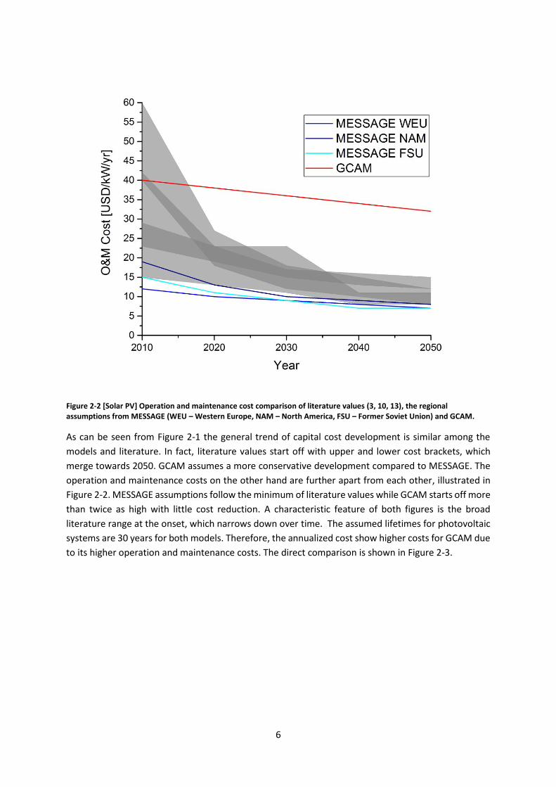
Figure 2-2 [Solar PV] Operation and maintenance cost comparison of literature values (3, 10, 13), the regional assumptions from MESSAGE (WEU – Western Europe, NAM – North America, FSU – Former Soviet Union) and GCAM.
As can be seen from Figure 2-1 the general trend of capital cost development is similar among the
models and literature. In fact, literature values start off with upper and lower cost brackets, which
merge towards 2050. GCAM assumes a more conservative development compared to MESSAGE. The
operation and maintenance costs on the other hand are further apart from each other, illustrated in
Figure 2-2. MESSAGE assumptions follow the minimum of literature values while GCAM starts off more
than twice as high with little cost reduction. A characteristic feature of both figures is the broad
literature range at the onset, which narrows down over time. The assumed lifetimes for photovoltaic
systems are 30 years for both models. Therefore, the annualized cost show higher costs for GCAM due
to its higher operation and maintenance costs. The direct comparison is shown in Figure 2-3.

7
Figure 2-3 [Solar PV] Annualized cost comparison of the regional assumptions from MESSAGE (WEU – Western Europe, NAM – North America, FSU – Former Soviet Union) and GCAM.

8
3 Concentrating Solar Power
3.1 Technical Description Concentrating solar power (CSP) systems use solar energy to generate electricity (or heat). The
underlying principle relies on the absorption of light by a receiving medium. The medium is generally
oil, air, water (steam) or liquid salt. The heated medium can then be used to power a thermodynamic
process to convert the thermal energy to electricity. This basic process is therefore very similar to
conventional power plants with the differentiator being the source of the heat. To save space and to
reach higher temperatures optical systems are used to focus sunlight from a large area to a smaller
receiving medium. Combining CSP plants with thermal storage systems allows them to generate
electricity even after sunset. Moreover, adding a combustion back-up system to generate heat makes
CSP plants potentially very reliable. (6)
3.2 Variations
3.2.1 Line focus
Parabolic trough and linear Fresnel reflectors are both systems that track the sun along one axis.
Fresnel reflectors consist of many flat mirrors that concentrate the light onto a tube through which the
receiving medium is pumped. Parabolic through systems use a parabolic reflector to focus light on a
tube and are the most developed technology. These line focusing technologies reach temperatures
between 290°C and 500°C and peak efficiencies ranging from 14% to 20%. (6, 14, 15)
3.2.2 Point focus
The reflectors in point focusing technologies track the sun along two axes. Solar power tower and dish
sterling systems use a point focus. A tower uses an array of reflectors to concentrate light onto the
receiving medium on top of the tower. A dish sterling system on the other hand contains a parabolic
reflector with a receiver placed in the focal point. Focal point technologies reach higher temperatures
in the range of 1000°C. Higher temperatures also lead to higher peak efficiencies between 23% and
31%. (6, 14, 15)
3.3 Outlook Technical improvements to achieve higher efficiencies and reduce costs are on the horizon. Developing
novel reflector optics, demonstrating large scale molten salts as heat transfer fluids for linear systems
and optimizing design choices for solar towers are all potential short-term improvements. Measures
such as introducing supercritical steam turbines to CSP plants or coupling them with PV technology via
spectrum splitting are also under investigation. (16)

9
3.4 Data Comparison
Figure 3-1 [Solar CSP] Capital cost comparison of literature values (10, 13, 16, 17), the regional assumptions from MESSAGE (WEU – Western Europe, NAM – North America, FSU – Former Soviet Union) and GCAM.

10
Figure 3-2 [Solar CSP] Operation and maintenance cost comparison of literature values (10, 13, 17, 18), the regional assumptions from MESSAGE (WEU – Western Europe, NAM – North America, FSU – Former Soviet Union) and GCAM.
The capital cost development depicted in Figure 3-1 highlights the regional diversity in MESSAGE. While
cost figures in Europe and North America are slightly decreasing there is an increase in capital costs in
the region of the former Soviet Union. By 2050 the cost values are aligned again, indicating a capital
cost harmonization over time. GCAM starts off with higher capital costs, which steadily decrease. This
development is in line with the literature trends. Figure 3-2 highlights the split in literature values,
which mainly results from the various storage options that lead to higher costs. Similar to the capital
cost development the FSU is increasing in costs until it reaches the other regions level. GCAM uses a
lower cost estimate, which remains lower than the MESSAGE assumptions over time. Factoring in the
expected lifetimes of 25 years in MESSAGE and 30 years in GCAM it becomes apparent that the cost
development is very similar in both models as can be seen in Figure 3-3. The major outlier is the Former
Soviet Union region with its lower starting costs.

11
Figure 3-3 [Solar CSP] Annualized cost comparison of the regional assumptions from MESSAGE (WEU – Western Europe, NAM – North America, FSU – Former Soviet Union) and GCAM.
12
4 Wind Power
4.1 Technical Description Wind energy can be harvested through the use of wind turbines. The air flow turns the blades of the
wind turbine where the kinetic energy of the wind is converted to rotational energy in the rotor. The
rotational energy is used to spin a generator so that electricity is produced. The theoretical maximum
efficiency of these turbines is 59% (in relation to the total kinetic energy of the wind passing the
turbine). This efficiency does not include further impacts like rotor friction or transmission losses.
There are two main types of turbines, horizontal and vertical axis turbines. Horizontal axis designs
dominate the market due to the superior efficiency and energy output. Wind turbines are generally
placed on towers to take advantage of stronger and less turbulent wind. The power output from wind
turbines can range from several kilowatts to megawatts, the most cost effective method is to group
them in larger wind farms, which provide electricity to the central grid. (6, 19, 20)
4.2 Variations
4.2.1 Onshore
Onshore wind turbines are typically mounted on towers between 50m to 100m high with rotor
diameters in the same region. Wind speeds are generally slower onshore and not as constant.
Moreover, wind direction changes occur frequently onshore. Since the turbine needs to face into the
wind this results in fewer optimal hours of operation. The investment and maintenance cost are
comparatively lower due to better the accessibility of the turbines on land and the milder
environmental impacts. (20, 21)
4.2.2 Offshore
Offshore wind power is a more recent development of wind energy conversion. The wind conditions
on sea are more favorable than on land because of the faster and more reliant air flow. Hence, offshore
wind farms are often larger in scale with higher rated capacity than onshore wind farms. The
construction and maintenance however is much more expensive than for onshore facilities. Offshore
turbines must be fixed to the seabed, withstand stronger winds and storms and are constantly
subjected to the erosive environment of the sea. As a result costs can be more than twice as high
compared to onshore equivalents. (20, 21)
4.3 Outlook While wind turbines are a very mature technology there is continued development to increase
efficiencies and decrease costs. Especially for offshore wind turbines where maintenance costs are
much higher the use of sensors and data analysis is becoming more popular. Monitoring factors like
moisture absorption or stress levels can help to predict failures and carry out maintenance works in
advance. This can save costs due to decreased downtimes and potentially bundling maintenance tasks.
The major technical challenge is the integration to the power grids due to stability problems. Therefore
grid infrastructure improvements are generally required to effectively use wind energy. (20, 22)

13
4.4 Data Comparison Please note that there was only wind onshore data available for comparison.
Figure 4-1 [Wind Onshore] Capital cost comparison of literature values (13, 17), the regional assumptions from MESSAGE (WEU – Western Europe, NAM – North America, FSU – Former Soviet Union) and GCAM.

14
Figure 4-2 [Wind Onshore] Operation and maintenance cost comparison of literature values (13, 17), the regional assumptions from MESSAGE (WEU – Western Europe, NAM – North America, FSU – Former Soviet Union) and GCAM.
From Figure 4-1 it can be seen that both models and the literature assume a general decline in capital
cost over time. However, MESSAGE assumptions start off lower than GCAM or the literature values.
GCAM’s cost estimates are between 35% and 90% higher than those from MESSAGE. The situation is
very similar for the operation and maintenance costs where MESSAGE values are at times half of those
from GCAM and slightly lower than the literature ranges between 2030 and 2045. Comparing the
annualized costs in Figure 4-3 confirms these observations (expected lifetimes of both models is 30
years). The assumptions for Western Europe are more aligned with GCAM than North America and the
Former Soviet Union region.

15
Figure 4-3 [Wind Onshore] Annualized cost comparison of the regional assumptions from MESSAGE (WEU – Western Europe, NAM – North America, FSU – Former Soviet Union) and GCAM.

16
5 Hydropower
5.1 Technical Description Hydropower plants harness energy from the natural water cycle by utilizing the water’s kinetic energy
to power a turbine. It is the most mature renewable energy technology to date and offers high
reliability, safety and is one of the most cost-effective power generation methods. Hydropower
produces around 16% of the global electricity output and makes up 80% of the global renewable
energy production. The capacity of hydropower plants can vary from several kW to hundreds of MW.
When compared to other renewable energy technologies hydropower yields a more constant power
output. Thus, it synergizes well with fluctuating power supplies from solar and wind. (23, 24)
5.2 Variations
5.2.1 Run-of-river
A run-of-river hydropower plant converts the available kinetic energy from the river flow to produce
electricity. They are further characterized by their lack of or very limited ability (hourly/daily) of storing
water and therefore energy. As a result, the power generation of run-of-river systems is highly
dependent on the flow rates of the river, making this option less reliable than other hydropower plants.
Thus, these systems are often built downriver of existing reservoirs to take advantage of the lower
construction costs while still retaining control over the power generation. (23, 24)
5.2.2 Reservoir
Hydropower plants are often associated with reservoirs, such as those behind dams. These reservoirs
have the capacity to store significant amounts of energy. This allows the decoupling of the power
generation from the highest water inflow periods, i.e. melting snow or heavy rain. This energy storage
makes reservoir hydropower plants one of the most flexible electricity suppliers and is ideal to facilitate
the integration of other variable renewable energy sources such as wind or solar. Another form of
hydropower plants that use reservoirs are pumped storage plants. Since these plants are technically
an energy storage option they are not listed here. (23, 24)
5.2.3 Tide
Tidal power generation uses the ocean’s water currents to power turbines. Tides are a result of the
gravitational attraction between the earth and the moon. Due to the constant orbit of the moon the
oceanic currents are also a constant energy source for tidal power plants. Energy conversion can be
either similar to wind turbines, i.e. using high current velocities to power the turbine, or similar to
pumped storage plants except that the process of elevating water uses natural sea level variations
instead of a pump. (25)
5.3 Outlook Even though hydropower is the most efficient power generation technology with turbine efficiency
above 90%, there is still some room for improvement. Developing technologies such as low kinetic flow
turbines for uses in canals, pipes or rivers is an example of such an improvement. It also shows that
the main restraint of hydropower plants is the limited land where plants can be built. So improving the
technologies that enable the use hydropower plants in locations that were thought to be inaccessible
will be a major focus. (23)

17
5.4 Data Comparison
Figure 5-1 [Hydro] Capital cost comparison of literature values (13, 24) and the regional assumptions from MESSAGE (WEU – Western Europe, NAM – North America, FSU – Former Soviet Union).
18
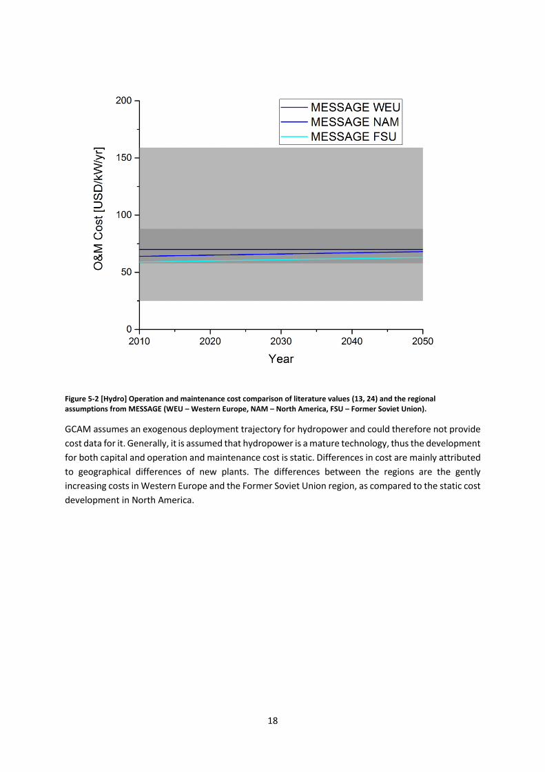
Figure 5-2 [Hydro] Operation and maintenance cost comparison of literature values (13, 24) and the regional assumptions from MESSAGE (WEU – Western Europe, NAM – North America, FSU – Former Soviet Union).
GCAM assumes an exogenous deployment trajectory for hydropower and could therefore not provide
cost data for it. Generally, it is assumed that hydropower is a mature technology, thus the development
for both capital and operation and maintenance cost is static. Differences in cost are mainly attributed
to geographical differences of new plants. The differences between the regions are the gently
increasing costs in Western Europe and the Former Soviet Union region, as compared to the static cost
development in North America.

19
Figure 5-3 [Hydro] Annualized cost comparison of the regional assumptions from MESSAGE (WEU – Western Europe, NAM – North America, FSU – Former Soviet Union) and GCAM.

20
6 Nuclear Power
6.1 Technical Description Nuclear power plants are thermal power plants that generate electricity in a similar manner to
conventional combustion type plants. The principle is that a fuel is reacted to heat the coolant, which
in turn heats water to create steam, which powers a turbine to generate electricity. The distinction of
nuclear power lies in the initial heat generation. Instead of burning a fuel to produce the heat a process
called nuclear fission is used. In a greatly simplified manner nuclear fission can be described as the
splitting of larger atoms into smaller atoms. In the case of nuclear power plants, the fissile material
(uranium or plutonium) is bombarded with neutrons to induce splitting. During the splitting energy
and further neutrons are released. The release of more neutrons is essential to reach a chain reaction
event so that the reaction is self-sustained. As of 2015 around 11% of the global electricity generation
came from nuclear power plants. (26, 27)
6.2 Variations
6.2.1 Light Water Reactors
Light water reactors use ordinary water as a coolant and moderator. The moderator is needed to slow
down neutrons to thermal energy levels making fission of uranium-235 more likely. Light water
reactors require enriched uranium fuel (a higher share of U-235 isotopes compared to U-238) to
sustain a chain reaction. There are two main types of light water reactors using either pressurized
water (PWR) or boiling water (BWR). In PWR’s the water to cool and moderate the reactor is kept at
high pressures so that it remains in its liquid form at elevated temperatures of over 300°C. The high-
pressure water heats water in a secondary loop to form steam and power the turbine. BWR’s in
contrast use only one loop where the water from the coolant and moderator is also the steam source
for the turbine. BWR’s are simpler to construct but less efficient. (28, 29)
6.2.2 Heavy Water Reactors
Heavy water reactors use deuterium oxide instead of ordinary water as a coolant and moderator.
Deuterium is an isotope of hydrogen that contains one more neutron. Heavy water, compared to light
water, absorbs fewer neutrons, which enables heavy water reactors to use non-enriched uranium as a
fuel. Therefore, there is a balance between the more expensive heavy water and the now much less
expensive fuel, since no enrichment facility is needed). The coolant is generally pressurized and a
steam generator is needed, similar to the design of PWR’s. (28)
6.2.3 Fast Breeder Reactors
A fast breeder reactor produces more new fuel than it consumes while operating. The reactor can
convert material that is generally fertile (not undergoing splitting) into fissile materials. This means for
example that the U-238 isotope in natural uranium can be converted to fissile plutonium. As a result,
the fuel economy of these reactors is much better that the conventional designs. To convert fertile
material to fissile material fast neutrons are required, therefore there is no need of a moderator and
the coolant should not be water since it slows neutrons down. Liquid metal is commonly used as a
coolant to overcome this. Due to higher operating temperatures the electricity production is more
efficient than that of conventional designs. (28)
21
6.3 Outlook Nuclear reactors can be categorized in terms of generations. The most common ones such as the light
and heavy water reactors are part of the second generation of nuclear reactors. Generation III are
mainly advanced versions of the second-generation reactor types. Current research focusses on
generation IV reactors with the aim of improving efficiency, safety, longevity and economic viability.
Fast breeder reactors are part of the fourth-generation research as well as very high temperature
reactors, a form of hybrid power plant where the heat will also be used to generate hydrogen. Other
reactor types of the fourth generation are the molten salt reactor (using a liquid fuel) and the super
critical water cooled reactor (operating above the critical point of water. (27, 28)
6.4 Data Comparison
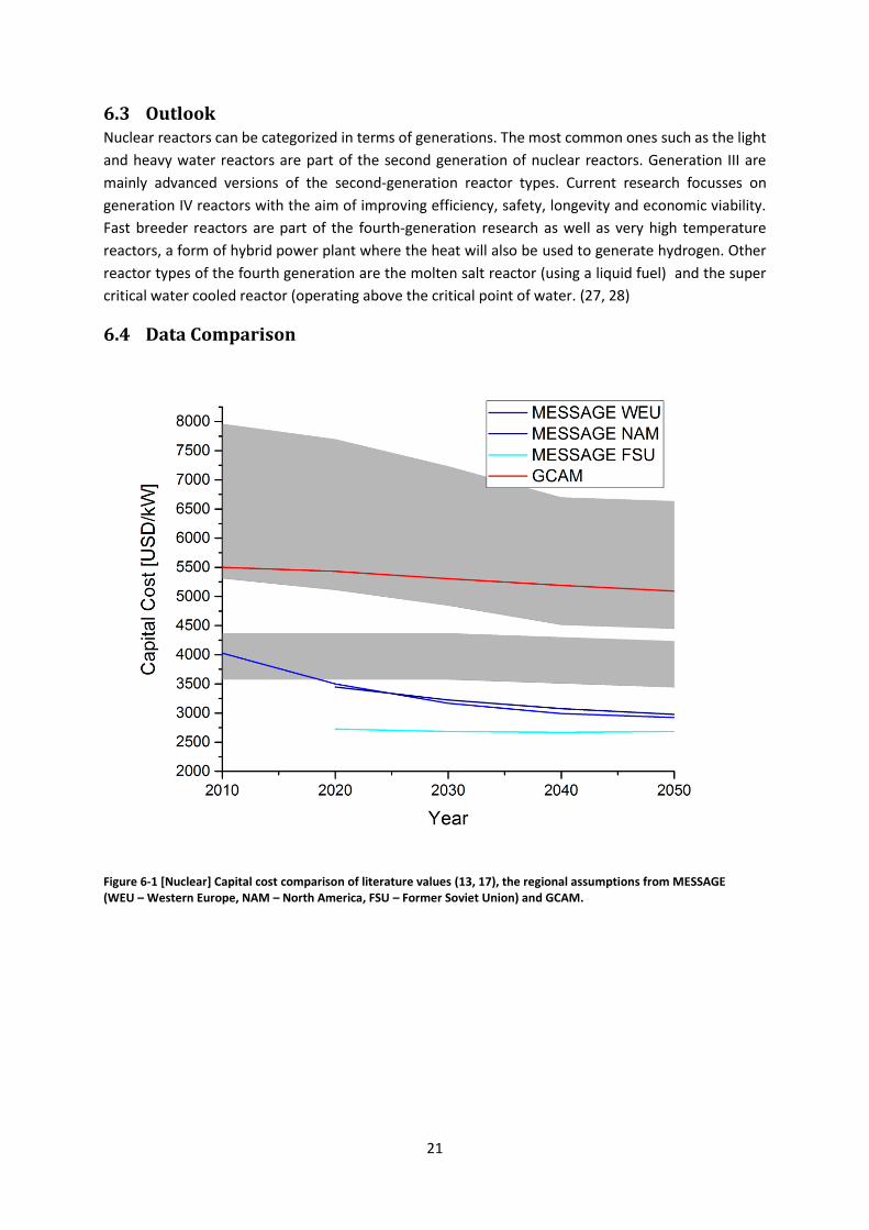
Figure 6-1 [Nuclear] Capital cost comparison of literature values (13, 17), the regional assumptions from MESSAGE (WEU – Western Europe, NAM – North America, FSU – Former Soviet Union) and GCAM.

22
Figure 6-2 [Nuclear] Operation and maintenance cost comparison of literature values (13, 17), the regional assumptions from MESSAGE (WEU – Western Europe, NAM – North America, FSU – Former Soviet Union) and GCAM.
Figure 6-1 illustrates differences among the regions in MESSAGE. Both, NAM and FSU only contain
cost figures after 2020. The capital cost assumptions from GCAM are up to 90% higher than those
from MESSAGE, which are generally lower than the literature values as well. Both models assume
decreasing costs over time, though MESSAGE values decrease at a faster rate. However, in Figure
6-2the situation is reversed. The operation and maintenance values from MESSAGE assumptions are
up to 90% higher than those from GCAM. GCAM’s higher capital cost, lower operation and
maintenance cost and equal lifetimes of 60 years compared to MESSAGE result in GCAM sitting in-
between the regional MESSAGE assumptions when it comes to the annualized cost. This can be seen
in Figure 6-3. MESSAGE’s Western Europe starts off 33% higher than GCAM, however, by 2050 all
model assumptions lie within a 10% range.

23
Figure 6-3 [Nuclear] Annualized cost comparison of the regional assumptions from MESSAGE (WEU – Western Europe, NAM – North America, FSU – Former Soviet Union) and GCAM.

24
7 Coal-Fueled Power Plants
7.1 Technical Description A coal fueled power plant converts heat energy into electrical energy, by turning water into steam,
which in turn drives turbine generators to produce electricity. First, flue gas is produced through the
combustion of pulverized coal. The thermal power of the flue gas is then used to turn water, pumped
through pipes inside a boiler, into steam. The pressure of the steam drives a steam turbine, that in turn
is connected to a generator that produces electricity. Conventional steam power plants operate at a
steam pressure in the range of 170 bar. These are subcritical power plants, which reach efficiencies up
to 38%. Both, lignite and hard coal are used as fuel. Hard coal power plants and lignite-fired power
plants have nearly identical plant facilities. While lignite-fired power plants are operated in base load,
hard coal power plants operate in the medium-load range. The pulverized coal type of boiler dominates
the electric power industry, producing about 50% of the world’s electricity supply (30, 31).
7.2 Variations
7.2.1 Lignite-and hard coal fired power plants
Lignite has a lesser burning capacity compared with hard coal as well as a greater water- and ash
content. Therefore, some lignite-fired power plant facilities are usually of larger dimensions. They can
achieve an efficiency factor up to 42%. Modern hard coal power plants achieve electrical efficiencies
of approx. 46% and advanced high-temperature power plants can even reach 50% (30, 31).
7.2.2 High-efficiency, low-emissions (HELE) coal-fired electricity generation
The term high-efficiency, low-emissions (HELE) comprises all plants within the coal-fired electricity
generation, which can reach a higher conversion efficiency and lower CO2 emissions intensity than
conventional subcritical coal-fired power plants through the usage of advanced technologies. These
technologies include super critical pulverized coal combustion, ultra-supercritical pulverized coal
combustion and integrated gasification combined cycle (IGCC) (32).
7.2.2.1 Super-critical, ultra-supercritical and advanced ultra-supercritical power plants
The difference between subcritical and supercritical versions of thermal power generation by coal is
associated with the steam pressure within the boiler. Higher steam pressure and temperature increase
the efficiency of the thermal cycle. In those conditions, steam is generated at a pressure above the
critical point of water, so no water-steam separation is required. Coal-fired plants with supercritical
technologies require less coal per MWh resulting in less greenhouse gas release, which leads to a
higher efficiency advantage in general (30).
Supercritical steam generators operate at pressures in the range of 220 to 275 bar and temperatures
of up to 600°C. They typically reach efficiencies of up to 42% (32). Ultra-super-critical power plants are
designed to operate at even higher temperature and pressure, which is made possible by the
development of materials with higher performance capabilities. Operating steam cycle conditions
above 539/621°C and at pressures of about 285 bar are referred to as ultra-supercritical. The
conversion efficiency of those power-plants amounts to 45%(33). Advanced ultra-supercritical coal
generation is under development and is expected to convert over 50% of the gross energy of coal to
electricity (33).

25
7.2.2.2 IGCC (Integrated Gasification Combined Cycle) power plants
In IGCC power plants, coal is conversed into pressurized gas, also called synthesis gas, using a high-
pressure gasifier. Under high temperature, coal is gasified with oxygen to generate synthesis gas, which
primarily consists of carbon monoxide, hydrogen and CO2. Other components are fuel-related
pollutants that are removed within a gas purification system. After purification, the synthesis gas is
utilized for electricity generation within a combined cycle natural gas turbine (also see 3.2.1). By
adding the higher-temperature steam produced by the gasification process the IGCC plant improves
the overall process efficiency. Moreover, an additional CO2-separation process can be integrated.
Through the water-gas shift reaction, carbon monoxide emissions are reduced by converting it to
carbon dioxide and hydrogen. The resulting CO2 from the shift reaction can be separated, compressed,
and stored through sequestration (30).
7.2.3 Desulphurization/DeNOx-Option
The flue gas generated in the combustion of coal contains other atmospheric pollutants like NOx
(oxides of nitrogen) and SOx (oxides of sulfur) in a concentration of about 15%. The terms
desulphurization and deNOx comprise a set of technologies used to remove those pollutants from
exhaust flue gases (30).
7.2.4 CHP (Combined Heat and Power)-Option
Cogeneration or combined heat and power (CHP) refers to the simultaneous generation of electricity
and heating from the combustion processes. Power plants using combined heat and power systems
recover the surplus heat produced from the electricity generation via heat exchangers. The regained
thermal energy can be used either on-site, be fed into a heat-storage device or into the district heating
network. CHP can therefor deliver savings in fuel consumption, fuel costs and carbon emissions. Power
generation plants with integrated CHP profit from a significantly increased annual efficiency and fuel
utilization rate (30).
7.2.5 CCS (Carbon Capture and Storage)-Option
Carbon capture and storage (CCS) technologies provide an opportunity for climate mitigation. Coal-
fired electricity generation with an attached CCS technology can be a possible measure to reduce
carbon emissions. In general, the CCS process can be divided into three stages: carbon dioxide capture,
transport and storage. To capture the CO2 from flue gas from coal-fired power plants there exist
several different industrial methods, which are explained below (30).
7.2.5.1 Post-combustion
In the post-combustion process, CO2 is removed through a chemical method from the flue gas
subsequently after flue gas purification (which includes desulphurization, denitrification and dust
extraction). Hereby CO2 is chemically bound to organic or anorganic liquid absorbents.
7.2.5.2 Pre-combustion
Coal gasification in coal-fired power plants can be combined with CO2 removal. The synthesis gas
generated in the gasification process contains CO2 and carbon monoxide (CO). In a carbon monoxide
shift reaction, CO is conversed to CO2 and hydrogen. Separation of CO2 is achieved by physical gas
washing procedure.
7.2.5.3 Oxyfuel
If the power plant burns coal with pure oxygen, the resulting flue gas consists only of water vapor and
high concentrated CO2 (about 80%). The separation takes place through the condensation of water

26
vapor from the flue gas. After compression, the largely pure CO2 can be transferred to the storage
location. The pure oxygen required for the combustion process can be produced in cryogenic air
separation units or membrane separation systems. Currently this process is highly energy consuming
which limits the broad application of the Oxyfuel technology. A potentially more efficient alternative
being explored to improve of Oxyfuel installations, is to use innovations in ceramic membranes for
oxygen separation at elevated temperatures. This method could lead to a 15% reduction in capital cost
(30) (34). R&D on the Oxyfuel process is carried out inter alia within the COORETEC research initiative
in the joint project ADECOS (Advanced Development of the coal fired Oxyfuel Process with CO2
Separation).
7.3 Outlook Although legitimate concerns about air pollution and greenhouse gas emissions are in public discourse,
coal remains an important energy source for power generation. The share of coal-fired power plants
in the global power production currently accounts for 40% (35).
For a carbon-constrained future, the usage of fossil fuel has to decrease and coal-fired power
generation would need to phase-out. The UN Sustainable Development Goals and Paris Agreement
renew pressures to take action towards a low-carbon transition. According to the OECD energy outlook
2017 (36), coal demand in Europe, USA and China has slightly decreased over the last two years and
the trend is expected to last. However, in many emerging economies, coal capacity is on the rise to
meet rapidly increasing energy demand. The future development of coal usage varies strongly by
region and is influenced by several factors, such as expected growth of demand and domestic access
to resources.
In the context of a sustainable energy future, the transition to higher efficiency power generation
through the implementation of HELE technologies is indispensable. 50% of constructed coal-fired
power plants in 2011 used HELE technologies (33). Still, according to IEA, about 30% of new installed
coal capacity in the years 2015 and 2016 accounted for subcritical technology (37). Concentrated
efforts to deploy and further develop HELE technology could essentially lower emissions from new
built or retrofitted coal-fired power plants. But at the same time the generation from older, less
efficient technology must gradually be phased out.
The development statues differ for the various HELE technologies - supercritical plants are mature
technology, ultra-supercritical plants are in deployment phase and ultra-supercritical plants are still in
development phase. IGCC units with efficiencies of about 45% are in deployment phase and until 2020
an efficiency factor of 50% is regarded as achievable. Advanced, higher firing temperature gas turbines
are still in the development phase (33).
To further decarbonize coal power generation and reach the global climate targets, the wide
implementation of CCS technologies will be essential. CCS received a lot of interest over the last 20
years but made limited progress to demonstrate commercial viability. One of the challenges is the
enormously energy intensive nature of common CCS technologies. CCS reduces a power plant’s
electricity output or increases its fuel input. This results in reduced efficiencies by up to 14%. To scale-
up new HELE and CCS technologies, effective funding and support mechanisms need to be provided as
well as mandatory policies have to be in place (33).

27
7.4 Data Comparison The following section gives an overview on the data comparison of the coal power generation
technologies IGCC, supercritical and subcritical power plants. For IGCC and supercritical technology the
first figures show the values for the option with included CCS technology.
7.4.1 IGCC with and without CCS
7.4.1.1 Capital Cost
As the figures above show, capital cost values taken from available literature for IGCC with CCS (Figure
7-1) and without CCS (Figure 7-2) spread widely. At the same time, there is a large gap between the
capital cost values used by MESSAGE and GCAM. The GCAM model assumes much higher capital cost
for IGCC with and without CCS, but the values coincide with the upper range of the literature data. The
model also assumes a linear capital cost reduction over time. In contrast, the values assumed by
MESSAGE are relatively low and beyond the capital cost range derived from the reviewed literature.
MESSAGE assumes the highest cost reduction for IGCC with or without CCS for the North American
regions until 2030 while the curves for the other two regions remain stable. CCS technologies in the
MESSAGE model are not included until 2020. The difference between the both models may result from
different assumptions in asset lifetime. In GCAM the lifetime for IGCC with or without CCS accounts for
60 years, while it is 30 years in MESSAGE.
Figure 7-1 [IGCC with CCS]Capital cost comparison of literature values (38, 39, 39–42), the regional assumptions from MESSAGE (WEU – Western Europe, NAM – North America, FSU – Former Soviet Union) and GCAM.
28
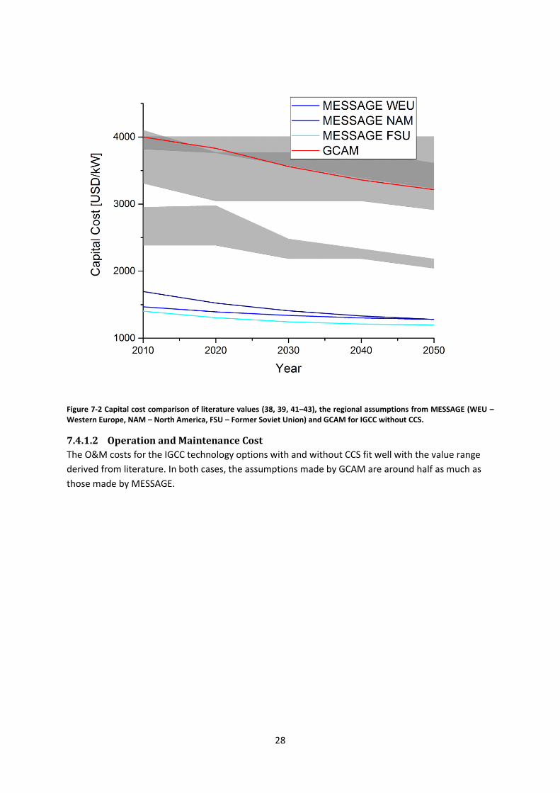
Figure 7-2 Capital cost comparison of literature values (38, 39, 41–43), the regional assumptions from MESSAGE (WEU – Western Europe, NAM – North America, FSU – Former Soviet Union) and GCAM for IGCC without CCS.
7.4.1.2 Operation and Maintenance Cost
The O&M costs for the IGCC technology options with and without CCS fit well with the value range
derived from literature. In both cases, the assumptions made by GCAM are around half as much as
those made by MESSAGE.

29
Figure 7-3 Operation and maintenance cost comparison of literature values (38, 41) and the regional assumptions from MESSAGE (WEU – Western Europe, NAM – North America, FSU – Former Soviet Union) for IGCC with CCS.

30
Figure 7-4 [IGCC without CCS] Operation and maintenance cost comparison of literature values (38, 41) and the regional assumptions from MESSAGE (WEU – Western Europe, NAM – North America, FSU – Former Soviet Union) for IGCC without CCS.
7.4.1.3 Efficiency
In contrast to GCAM, the MESSAGE model doesn’t include a change rate over the years. For IGCC
with CCS he efficiency value from MESSAGE is 10% below the literature range while the mean value
of GCAM fits well into the defined range. Still, it shares approximately the same start value as
MESSAGE for 2010. This is also true for the figure of IGCC without CCS. Here, the values for both
models are consistent with the reviewed literature.

31
Figure 7-5 [IGCC with CCS] Efficiency comparison of literature values (41, 42) and the regional assumptions from MESSAGE (WEU – Western Europe, NAM – North America, FSU – Former Soviet Union)

32
Figure 7-6 [IGCC without CCS] Efficiency comparison of literature values (39, 42, 44) and the regional assumptions from MESSAGE (WEU – Western Europe, NAM – North America, FSU – Former Soviet Union).
7.4.2 Supercritical power plants with and without CCS
7.4.2.1 Capital Cost
The reviewed literature data for supercritical technology also show a broad spectrum of the projected
development of capital costs. Supercritical technology can generally have very different properties
which results in the cost variations. Both models lie within this range but on the opposite sides of the
spectrum. MESSAGE does not include supercritical technology until 2020 and capital costs are more
than a half lower than the costs assumed by the GCAM model. Both models have also differences in
their technology lifetime assumptions. Here, same applies as for IGCC - the lifetime of supercritical
technology within the GCAM model is 60 years, while it is 30 years within MESSAGE.

33
Figure 7-7 [Supercritical power plants with CCS]Capital cost comparison of literature values (38, 39, 41–43), the regional assumptions from MESSAGE (WEU – Western Europe, NAM – North America, FSU – Former Soviet Union).

34
Figure 7-8 [Supercritical power plants without CCS] Capital cost comparison of literature values (38, 39, 41–44), the regional assumptions from MESSAGE (WEU – Western Europe, NAM – North America, FSU – Former Soviet Union).
7.4.2.2 Operation and Maintenance Cost
There is also an obvious gab in operation and maintenance costs between GCAM and MESSAGE. Here
the effect is reverse compared to the capital cost, and GCAM calculates with lower values than
MESSAGE. For supercritical installations with CCS GCAM fits well into the ranged derived from the
reviewed literature. MESSAGE assumes values on the upper range for the FSU region for the year 2020
and even higher costs for the NAM and WEU regions. By 2050 all cost curves meet the range of
literature values. With regard to supercritical technology without CCS, the literature sources showed
two different ranges. While the GCAM cost curve falls into the lower range, the MESSAGE values fall
into the upper one.

35
Figure 7-9 [Supercritical power plants with CCS] Operation and maintenance cost comparison of literature values (38, 41) and the regional assumptions from MESSAGE (WEU – Western Europe, NAM – North America, FSU – Former Soviet Union) for supercritical technology with CCS.

36
Figure 7-10 [Supercritical power plants without CCS] Operation and maintenance cost comparison of literature values (38, 39, 41, 44) and the regional assumptions from MESSAGE (WEU – Western Europe, NAM – North America, FSU – Former Soviet Union) for supercritical technology without CCS.

37
7.4.2.3 Efficiency
The literature sources on efficiency of supercritical technology with combined CCS were limited.
According to IEA Efficiency might improve to 41 to 46%. MESSAGE assumes a constant value of 35%.
GCAM starts with a value of 32% for 2010 and assumes a linear increase in efficiency over the following
decades to reach a value of 0,56 by 2050. Energy efficiency of power plants with carbon capture and
storage diminish significantly. More literature data is available on supercritical technology without CCS.
As shown in Figure 7-12, MESSAGE and GCAM values are within the literature range. Here, MESSAGE
uses a constant value of 37% while GCAM assumes an efficiency of 41% in 2010 and ascends to 55% in
2050.
Figure 7-11 [Supercritical power plants with CCS] Efficiency comparison of literature values (41, 42) and the regional assumptions from MESSAGE (WEU – Western Europe, NAM – North America, FSU – Former Soviet Union).
38
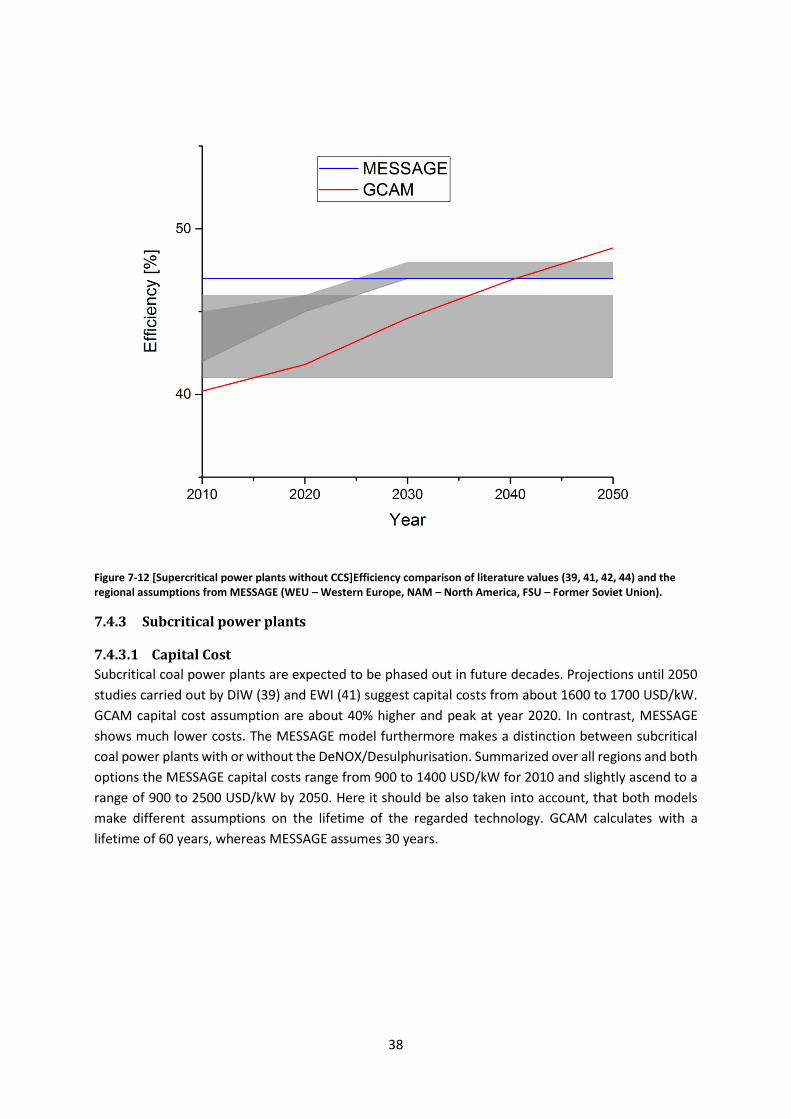
Figure 7-12 [Supercritical power plants without CCS]Efficiency comparison of literature values (39, 41, 42, 44) and the regional assumptions from MESSAGE (WEU – Western Europe, NAM – North America, FSU – Former Soviet Union).
7.4.3 Subcritical power plants
7.4.3.1 Capital Cost
Subcritical coal power plants are expected to be phased out in future decades. Projections until 2050
studies carried out by DIW (39) and EWI (41) suggest capital costs from about 1600 to 1700 USD/kW.
GCAM capital cost assumption are about 40% higher and peak at year 2020. In contrast, MESSAGE
shows much lower costs. The MESSAGE model furthermore makes a distinction between subcritical
coal power plants with or without the DeNOX/Desulphurisation. Summarized over all regions and both
options the MESSAGE capital costs range from 900 to 1400 USD/kW for 2010 and slightly ascend to a
range of 900 to 2500 USD/kW by 2050. Here it should be also taken into account, that both models
make different assumptions on the lifetime of the regarded technology. GCAM calculates with a
lifetime of 60 years, whereas MESSAGE assumes 30 years.

39
Figure 7-13 [Subcritical power plants] Capital cost comparison of literature values (39, 42), the regional assumptions from MESSAGE (WEU – Western Europe, NAM – North America, FSU – Former Soviet Union) and GCAM.
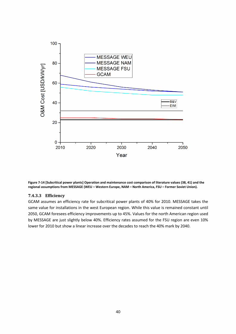
7.4.3.2 Operation and Maintenance Cost
GCAM assumptions on operation and maintenance costs of subcritical coal power plants fit perfectly
with the values proposed by Black and Veatch (38). The operation and maintenance costs from
MESSAGE are more than twice as high.
40
Figure 7-14 [Subcritical power plants] Operation and maintenance cost comparison of literature values (38, 41) and the regional assumptions from MESSAGE (WEU – Western Europe, NAM – North America, FSU – Former Soviet Union).
7.4.3.3 Efficiency
GCAM assumes an efficiency rate for subcritical power plants of 40% for 2010. MESSAGE takes the
same value for installations in the west European region. While this value is remained constant until
2050, GCAM foresees efficiency improvements up to 45%. Values for the north American region used
by MESSAGE are just slightly below 40%. Efficiency rates assumed for the FSU region are even 10%
lower for 2010 but show a linear increase over the decades to reach the 40% mark by 2040.
41
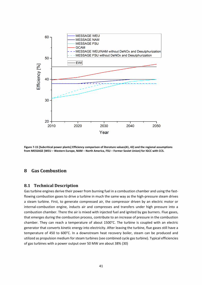
Figure 7-15 [Subcritical power plants] Efficiency comparison of literature values(41, 42) and the regional assumptions from MESSAGE (WEU – Western Europe, NAM – North America, FSU – Former Soviet Union) for IGCC with CCS.
8 Gas Combustion
8.1 Technical Description Gas turbine engines derive their power from burning fuel in a combustion chamber and using the fast-
flowing combustion gases to drive a turbine in much the same way as the high-pressure steam drives
a steam turbine. First, to generate compressed air, the compressor driven by an electric motor or
internal-combustion engine, inducts air and compresses and transfers under high pressure into a
combustion chamber. There the air is mixed with injected fuel and ignited by gas burners. Flue gases,
that emerges during the combustion process, contribute to an increase of pressure in the combustion
chamber. They can reach a temperature of about 1500°C. The turbine is coupled with an electric
generator that converts kinetic energy into electricity. After leaving the turbine, flue gases still have a
temperature of 450 to 600°C. In a downstream heat recovery boiler, steam can be produced and
utilized as propulsion medium for steam turbines (see combined cycle gas turbine). Typical efficiencies
of gas turbines with a power output over 50 MW are about 38% (30)

42
8.2 Variations
8.2.1 Gas steam power
The most basic natural gas-fired electric generation consists of a steam generation unit, where fuels
are burned in a boiler to heat water and produce steam that then turns a turbine to generate
electricity. Natural gas may be used for this process. Typically, only 33 to 35% of the thermal energy
used to generate the steam is converted into electrical energy in these types of plants (30).
8.2.2 Combined cycle gas turbine (CCGT)
When a natural gas-fired turbine is combined with heat recovery steam generators to produce steam,
significant improvements can be realized in both efficiency and electrical output. This configuration is
referred to as combined cycle gas turbine (CCGT). Usually about two-thirds of the total power is
produced from the gas turbines and one-third from the steam cycle. The gas turbine generates
electricity directly and the system harnesses waste heat to create steam, which powers a steam
turbine. Because of this efficient use of the heat energy released from the natural gas, combined-cycle
plants are much more efficient, than gas turbines alone. Combined cycle plants can achieve thermal
efficiencies of up to 50 to 60% (30, 45).
8.3 Outlook Currently natural gas has a share of 25% of electricity generation (46). Natural gas is a lower-carbon
alternative to gas-fired power generation and is under discussion as a bridging technology to provide
short-term support for the integration of renewables. But at the same time gas is also increasingly
competing with renewable power generation technologies (46). Gas turbine power generation is
primarily used for peak-load demands, as it is possible to quickly and easily turn them on. These plants
have increased popularity due to advances in technology and the availability of natural gas (30).
Performance and efficiency of gas turbines were increased successively over the last two decades. CCG
power generation plants operate with an efficiency of about 60%. The aim is to reach an efficiency
factor of up to 65% within the next decade (47). CCG is projected to become the cheapest fossil-fuel
baseload technology. Higher efficiencies are likely to be reached through usage of new materials and
innovative coatings for the high-temperature components of the gas turbine to further increase
turbine inlet temperatures. Just like in coal-fired power plants CCS (see chapter 8.2.5) can be included
in the technology outline to reach further emission cuts (30).
8.4 Data Comparison The following section gives an overview on the data comparison of the power generation from gas
combustion. The selected technologies are GCC with and without CCS, gas steam power plant and gas
turbine power plant. The latter two are pictured in one chapter as no differentiation for the reviewed
values was made by GCAM.
8.4.1 Gas combined cycle power plant with and without CCS
8.4.1.1 Capital Cost
According to the literature review, the projected capital cost values for combined cycle with CCS vary
widely. The GCAM values fall within the determined range. Capital cost values provided by MESSAGE
in comparison are only half as large and are slightly beyond the lower range of the literature spectrum.
For combined cycle technology without CCS the literature values overlap and capital costs range from
900 to 1250 USD/kW. Here, GCAM and MESSAGE do not meet with this range and assume lower capital

43
costs. Still the assumptions made by GCAM are about twice as high as those made by MESSAGE.
Furthermore, GCAM foresees a peak in capital costs by 2020. Lifetime used by GCAM for these
technologies is 45 years, while MESSAGE calculates with 30 years.
Figure 8-1 [Gas combined cycle with CCS] Capital cost comparison of literature values (39, 42), the regional assumptions from MESSAGE (WEU – Western Europe, NAM – North America, FSU – Former Soviet Union).

44
Figure 8-2 [Gas combined cycle without CCS] Capital cost comparison of literature values (39, 42), the regional assumptions from MESSAGE (WEU – Western Europe, NAM – North America, FSU – Former Soviet Union) and GCAM for combined cycle technology without CCS.
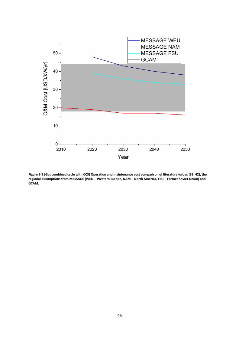
8.4.1.2 Operation and Maintenance Cost
Operation and maintenance costs for combined cycle with or without CCS from GCAM and MESSAGE
are consistent with the range derived from the literature review. In both cases the assumptions
made by MESSAGE are higher than those made by GCAM.
45
Figure 8-3 [Gas combined cycle with CCS] Operation and maintenance cost comparison of literature values (39, 42), the regional assumptions from MESSAGE (WEU – Western Europe, NAM – North America, FSU – Former Soviet Union) and GCAM.
46
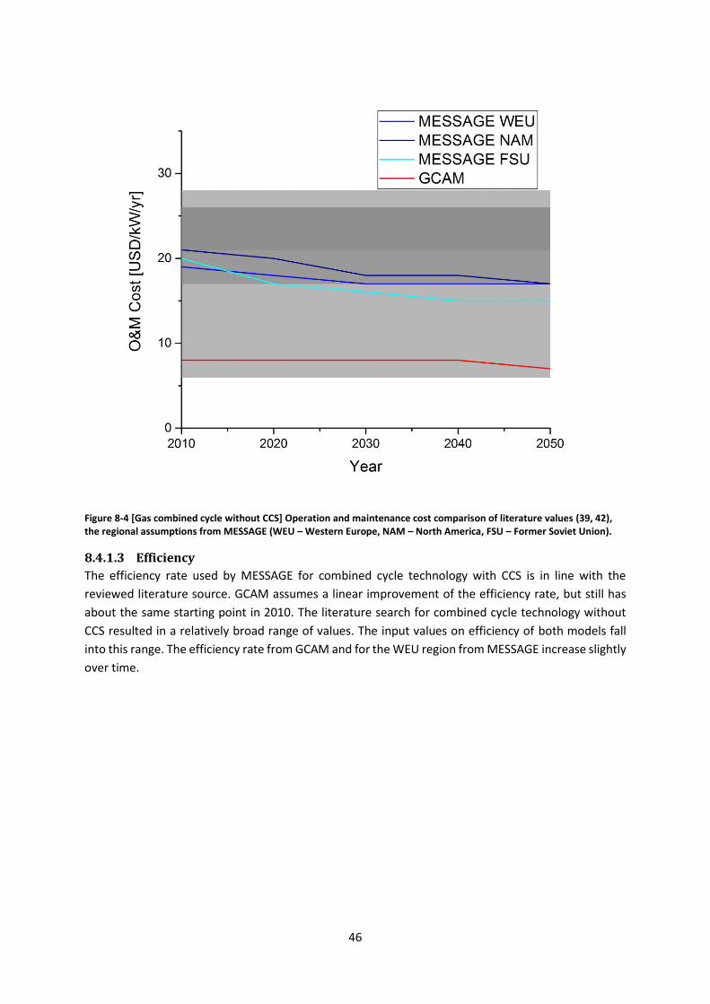
Figure 8-4 [Gas combined cycle without CCS] Operation and maintenance cost comparison of literature values (39, 42), the regional assumptions from MESSAGE (WEU – Western Europe, NAM – North America, FSU – Former Soviet Union).
8.4.1.3 Efficiency
The efficiency rate used by MESSAGE for combined cycle technology with CCS is in line with the
reviewed literature source. GCAM assumes a linear improvement of the efficiency rate, but still has
about the same starting point in 2010. The literature search for combined cycle technology without
CCS resulted in a relatively broad range of values. The input values on efficiency of both models fall
into this range. The efficiency rate from GCAM and for the WEU region from MESSAGE increase slightly
over time.

47
Figure 8-5 [Gas combined cycle with CCS] Efficiency comparison of literature values (41) and the regional assumptions from MESSAGE (WEU – Western Europe, NAM – North America, FSU – Former Soviet Union).
48
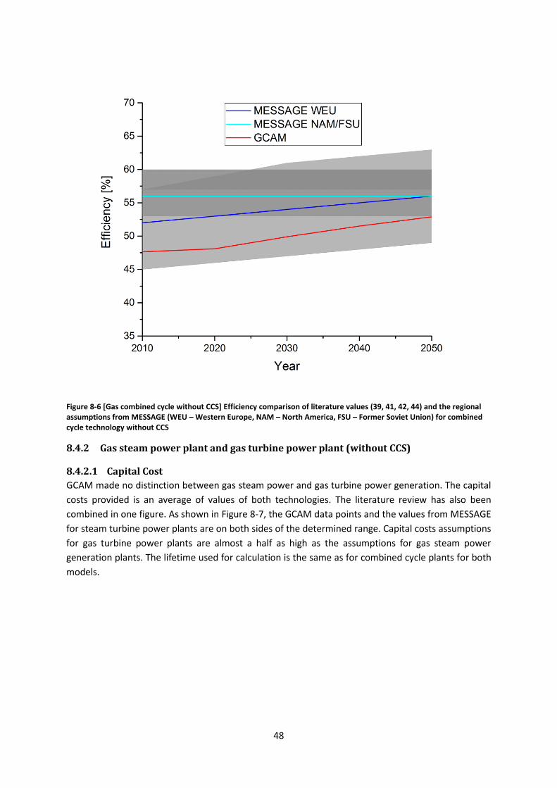
Figure 8-6 [Gas combined cycle without CCS] Efficiency comparison of literature values (39, 41, 42, 44) and the regional assumptions from MESSAGE (WEU – Western Europe, NAM – North America, FSU – Former Soviet Union) for combined cycle technology without CCS
8.4.2 Gas steam power plant and gas turbine power plant (without CCS)
8.4.2.1 Capital Cost
GCAM made no distinction between gas steam power and gas turbine power generation. The capital
costs provided is an average of values of both technologies. The literature review has also been
combined in one figure. As shown in Figure 8-7, the GCAM data points and the values from MESSAGE
for steam turbine power plants are on both sides of the determined range. Capital costs assumptions
for gas turbine power plants are almost a half as high as the assumptions for gas steam power
generation plants. The lifetime used for calculation is the same as for combined cycle plants for both
models.
49
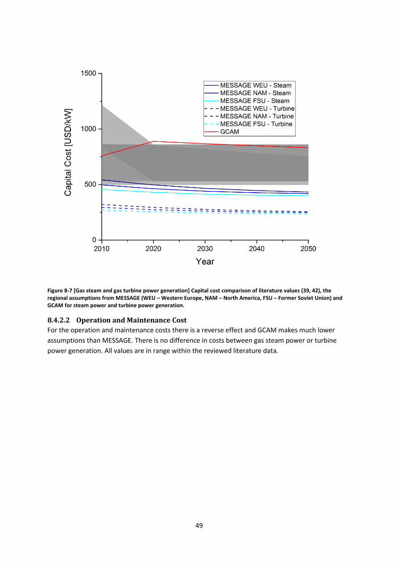
Figure 8-7 [Gas steam and gas turbine power generation] Capital cost comparison of literature values (39, 42), the regional assumptions from MESSAGE (WEU – Western Europe, NAM – North America, FSU – Former Soviet Union) and GCAM for steam power and turbine power generation.
8.4.2.2 Operation and Maintenance Cost
For the operation and maintenance costs there is a reverse effect and GCAM makes much lower
assumptions than MESSAGE. There is no difference in costs between gas steam power or turbine
power generation. All values are in range within the reviewed literature data.

50
Figure 8-8 [Gas steam and gas turbine power generation] Operation and maintenance cost comparison of literature values (39, 42), the regional assumptions from MESSAGE (WEU – Western Europe, NAM – North America, FSU – Former Soviet Union) and GCAM for steam power and turbine power generation.
9 Biomass
9.1 Technical Description Biomass is defined as carbonaceous materials derived from organic naturally grown substances. It can
be divided into (1) primary products, like plants, plant residues, agricultural or forestry products and
(2) secondary products as animal waste or municipal sludge. The energy uses of biomass cover biomass
combustion and conversion of biomass to biofuel. Agriculture and forestry residues, and in particular
residues from timber and paper mills, are the most common biomass resources used for generating
electricity. Since biomass raw material absorbs CO2 from the atmosphere during plant growth,
biomass combustion is considered as CO2 neutral. Biomass can be converted into other energy carriers
through thermo-chemical, thermo-physical or bio-chemical processes. The composition of biomass, as
the water, oxygen or ash content, has an influence on the heating value that is a crucial factor for the
energy that can be provided. Most of today's biomass power plants are direct-fired systems. For power
generation biomass is burned in direct or co-fired systems for generating steam. In addition to
combustion, biomass can be converted to biofuels (30).

51
9.2 Variations
9.2.1 Biomass steam power plant
Direct biomass power plants use the heat generated during the combustion process is used to fire a
boiler. The resulting is driving steam turbines to produce electricity. The properties and composition
of the specific biomass materials used for power generation are essential. Some biomass requires
preceding pre-treatment. The biomass combustion process is divided in three stages – heating and
drying, pyrolysis, gasification and oxidation. The different stages take place in different temperature
ranges. Heating and drying is aimed at the expulsion of water from the biomass feedstock. The water
content of the utilized biomass drives this process. In the following pyrolysis the thermal
decomposition under the absence of air sets in. Here, the long-chain hydro-carbs are broken down.
During the gasification process, synthesis gas is created at high temperatures. Through combustion of
the synthesis gas in the oxidation process the heat for driving the boiler is generated (30, 48).
9.2.2 Biomass IGCC power plant
Biomass IGCC has the same technological approach as the pulverized coal IGCC technology (see 2.2.2).
However, because of the specific properties of the biomass feedstock several technological
adjustments are required. At best, BIGCC technology is combined with subsequent CCS technology to
reach net negative emissions. Currently there are some demonstration BIGCC projects ongoing but
large scale power generation through biomass gasification needs further technological innovations and
planning for biomass supply (49).
9.2.3 Co-firing
Co-firing is the practice of firing biomass fuels as a supplement to fossil fuels as in a conventional power
generation plants. Whereby co-firing does not contribute additional capacity, but instead displaces the
fossil fuel by unit. In pulverized coal power plants, biomass is either blended with coal on the conveyor
belt feeding the coal bunkers (only applicable for biomass from wood), or separately injected into the
furnace (30). Co-firing of 5%-10% biomass of the total load usually requires minor changes in the
handling equipment. A biomass share of over 10% would lead to changes in mills, burners and dryers
(50). Co-firing is mature technology and widely applied in modern coal-fired power plants.
9.3 Outlook Bioenergy in general has the largest among renewable energy sources. However, the cultivation of
biomass can entail land use change, if the area affected was not or otherwise used beforehand. Land-
use changes can have an impact on the lifecycle assessment of biomass-derived products.
Furthermore, it should be taken into account that cultivation and processing require energy input that
are not necessarily considered CO2-neutral. Because of the varieties in sources of biomass and
different handling processes and pre-treatment requirements, the costs of biomass generated power
can fluctuate significantly (30). Co-firing and direct biomass power plants are already widely deployed,
other promising technologies as BIGCC are not commercialized. Competitiveness of advanced
technologies will mostly depend on future regulations and prices of CO2 emissions(49).
9.4 Data Comparison The following section gives an overview on the data comparison of the power generation technologies
biomass steam power and biomass IGCC (with and without CCS).

52
9.4.1 Biomass IGCC and biomass steam power plants
9.4.1.1 Capital Cost
Figure 9-2 shows the capital cost values used by MESSAGE and GCAM for biomass IGCC technology
with and without CCS. GCAM makes significantly higher assumptions on capital cost values than
MESSAGE for both options. Capital costs for biomass IGCC with CCS drop around 25% from 2010 to
2050. Biomass IGCC technology without CCS has about 40% lower capital costs according to GCAM.
MESSAGE does not include biomass IGCC power plants with CCS until 2030. Biomass IGCC capital costs
with or without CCS are about one third of the corresponding values used by GCAM.
In Figure 9-3 the capital cost input values are compared for steam power generation technologies.
GCAM and MESSAGE assumptions are on opposite sides of the spectrum for capital costs derived from
literature. However, for all technology options MESSAGE assumes a lifetime of 25 years, whereas it is
60 years for GCAM.
Figure 9-1 [Biomass IGCC with and without CCS]Capital cost comparison of, the regional assumptions from MESSAGE (WEU – Western Europe, NAM – North America, FSU – Former Soviet Union).

53
Figure 9-2 [Biomass steam power]Capital cost comparison of literature values (38, 39, 41), the regional assumptions from MESSAGE (WEU – Western Europe, NAM – North America, FSU – Former Soviet Union) and GCAM..
9.4.1.2 Operation and Maintenance Cost
Figure 9-4 shows the comparison of operation and maintenance costs for biomass IGCC with CCS. The
costs from GCAM show a linear decrease of about 25%. MESSAGE does not include CCS technology
until 2030. O&M costs for the North American region are the highest. Still on average, the MESSAGE
assumptions GCAM values are about 25% lower for 2030 and 2050.
For biomass IGCC power plant without CCS and biomass steam power plant without CCS GCAM and
MESSAGE use the same values for operation and maintenance costs. Therefore, Figure 9-5 summarizes
the results for both technologies in one image. Literature data ranges widely from 50 USD/kW to 350
USD/kW.

54
Figure 9-3 [Biomass IGCC with CCS]Operation and maintenance cost comparison of the regional assumptions from MESSAGE (WEU – Western Europe, NAM – North America, FSU – Former Soviet Union) and GCAM. No literature values available.
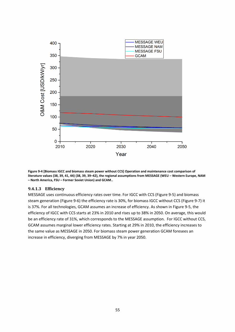
55
Figure 9-4 [Biomass IGCC and biomass steam power without CCS] Operation and maintenance cost comparison of literature values (38, 39, 41, 44) (38, 39, 39–42), the regional assumptions from MESSAGE (WEU – Western Europe, NAM – North America, FSU – Former Soviet Union) and GCAM..
9.4.1.3 Efficiency
MESSAGE uses continuous efficiency rates over time. For IGCC with CCS (Figure 9-5) and biomass
steam generation (Figure 9-6) the efficiency rate is 30%, for biomass IGCC without CCS (Figure 9-7) it
is 37%. For all technologies, GCAM assumes an increase of efficiency. As shown in Figure 9-5, the
efficiency of IGCC with CCS starts at 23% in 2010 and rises up to 38% in 2050. On average, this would
be an efficiency rate of 31%, which corresponds to the MESSAGE assumption. For IGCC without CCS,
GCAM assumes marginal lower efficiency rates. Starting at 29% in 2010, the efficiency increases to
the same value as MESSAGE in 2050. For biomass steam power generation GCAM foresees an
increase in efficiency, diverging from MESSAGE by 7% in year 2050.
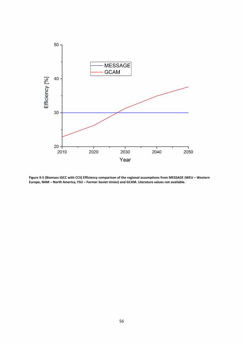
56
Figure 9-5 [Biomass IGCC with CCS] Efficiency comparison of the regional assumptions from MESSAGE (WEU – Western Europe, NAM – North America, FSU – Former Soviet Union) and GCAM. Literature values not available.

57
Figure 9-6 [Biomass IGCC without CCS] Efficiency comparison of literature values (44), the regional assumptions from MESSAGE (WEU – Western Europe, NAM – North America, FSU – Former Soviet Union) and GCAM for biomass IGCC without CCS.
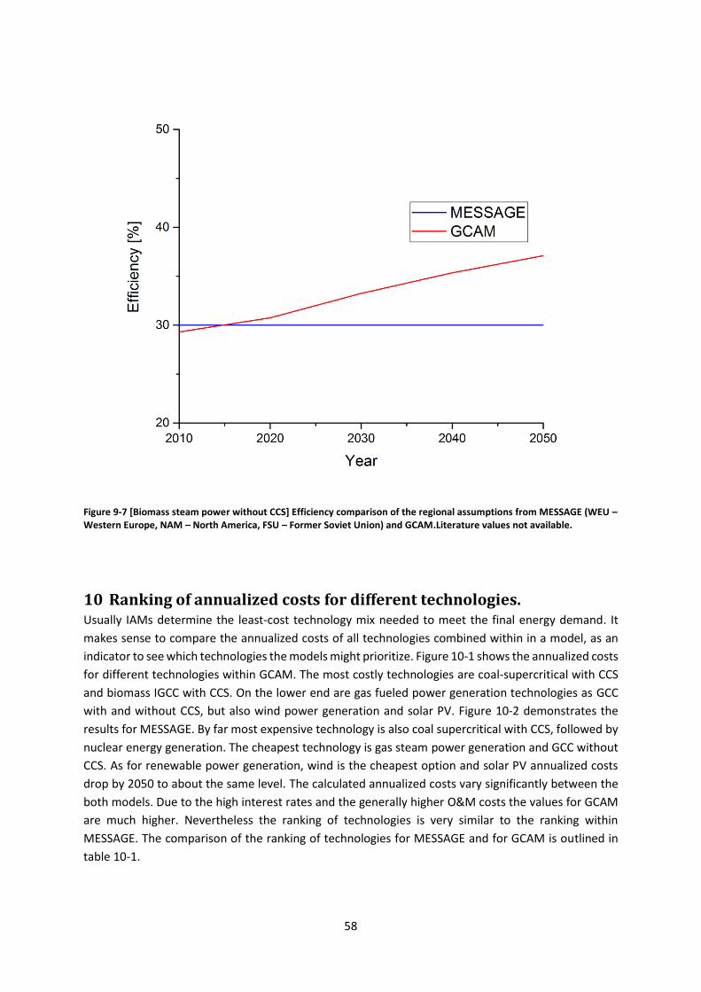
58
Figure 9-7 [Biomass steam power without CCS] Efficiency comparison of the regional assumptions from MESSAGE (WEU – Western Europe, NAM – North America, FSU – Former Soviet Union) and GCAM.Literature values not available.
10 Ranking of annualized costs for different technologies. Usually IAMs determine the least-cost technology mix needed to meet the final energy demand. It
makes sense to compare the annualized costs of all technologies combined within in a model, as an
indicator to see which technologies the models might prioritize. Figure 10-1 shows the annualized costs
for different technologies within GCAM. The most costly technologies are coal-supercritical with CCS
and biomass IGCC with CCS. On the lower end are gas fueled power generation technologies as GCC
with and without CCS, but also wind power generation and solar PV. Figure 10-2 demonstrates the
results for MESSAGE. By far most expensive technology is also coal supercritical with CCS, followed by
nuclear energy generation. The cheapest technology is gas steam power generation and GCC without
CCS. As for renewable power generation, wind is the cheapest option and solar PV annualized costs
drop by 2050 to about the same level. The calculated annualized costs vary significantly between the
both models. Due to the high interest rates and the generally higher O&M costs the values for GCAM
are much higher. Nevertheless the ranking of technologies is very similar to the ranking within
MESSAGE. The comparison of the ranking of technologies for MESSAGE and for GCAM is outlined in
table 10-1.

59
Figure 10-1 Annaulized costs of the selected technologies from 2010-2050 as projected by GCAM
Figure 10-2 Annaulized costs of different technologies from 2010-2050 as projected by MESSAGE

60
Table 10-1 Comparison of the ranking of the annualized costs of different technologies between GCAM and MESSAGE
GCAM Ranking 2050 MESSAGE
Technology lowest first Technology
Gas Steam 1 1 Gas Turbine
Gas Turbine 1 2 GCC
GCC 1 3 Gas Steam
PV 4 4 Wind
GCC w/CCS 5 5 PV
Wind 6 6 GCC w/CCS
Coal Subcritical 7 7 Coal Subcritical
Coal IGCC 8 8 Coal IGCC
CSP 9 9 Biomass Steam
Biomass Steam 10 10 Biomass IGCC
Biomass IGCC 10 11 Coal IGCC w/CCS
Nuclear 12 12 CSP
13 Hydro
Coal IGCC w/CCS 13 14 Biomass IGCC w/CCS
Biomass IGCC w/CCS 14 15 Nuclear
Coal Super Critical w/CCS 15 16 Coal Super Critical w/CCS
The comparison of the annualized costs shows, that both models have a very similar prioritization
when it comes to the selected power generation technologies for this report. The similar relation of
technologies of both models. Still, it should be noted that this comparison is based on a very simple
analysis of the input parameters only. IAMs include a higher technological detail within the calculation
and there is high number of variations in technological options that is added in the model runs. Also,
the comparison above does not take into account fuel prices, which would also have a high impact on
the overall results:
61
11 Literature Cited 1. IIASA. The MESSAGEix framework [cited 2018 Jun 21]. Available from: URL:
https://messageix.iiasa.ac.at/index.html.
2. JGCRI. GCAM v4.4 Documentation: Global Change Assessment Model (GCAM) [cited 2018 Jun 21].
Available from: URL: http://jgcri.github.io/gcam-doc/.
3. International Energy Agency - IEA. Technology Roadmap Solar Photovoltaic Energy; 2010.
4. Phillips S, Warmuth W. Photovoltaics Report 2016: Fraunhofer Institute for Solar Energy; 2016.
5. Statista. Market share of global solar photovoltaics from 2011 to 2015, by technology; 2017 [cited
2017 Jun 22].
6. Wietschel M, Arens M, Doetsch C, Herkel S, Krewitt W, Markewitz P et al. Energietechnologien
2050: Fraunhofer Verlag; 2010.
7. Cheng P, Zhan X. Stability of organic solar cells: Challenges and strategies. Chemical Society
reviews 2016; 45(9):2544–82.
8. Hoppe H, Sariciftci NS. Organic solar cells: An overview. Journal of Materials Research 2004;
19(7):1924–45.
9. Conibeer G. Third-generation photovoltaics. Materials Today 2007; 10(11):42–50.
10. Schröder A, Kunz F, Meiss M, Mendelevitch R, von Hirschhausen C. Current and Prospective Costs
of Electricity Generation until 2050: Deutsches Institut für Wirtschaftsforschung; 2013.
11. National Renewable Energy Laboratory - NREL. Photovoltaic System Pricing Trends: Historical,
Recent, and Near-Term Projections (Presentation): U.S. Department of Energy; 2014.
12. Mayer J. Current and Future Cost of Photovoltaics: Fraunhofer Institute for Solar Energy; 2015.
13. Joint Research Centre. ETRI - Energy Technology Reference Indicator projections for 2010-2050:
European Commission; 2014.
14. Liu M, Steven Tay NH, Bell S, Belusko M, Jacob R, Will G et al. Review on concentrating solar
power plants and new developments in high temperature thermal energy storage technologies.
Renewable and Sustainable Energy Reviews 2016; 53:1411–32.
15. Lovegrove K, Stein W. Concentrating solar power technology: Principles, developments and
applications: Elsevier; 2012.
16. International Energy Agency - IEA. Technology Roadmap Solar Thermal Electricity 2014.
17. European Climate Foundation - ECF. Roadmap 2050: a practical guide to a prosperous, low-
carbon Europe; 2010.
18. International Renewable Energy Agency - IRENA. Renewable Energy Technologies Cost Analysis
Series: Concentrating Solar Power; 2012.
19. Department of Energy. Wind Turbines [cited 2017]. Available from: URL:
https://energy.gov/eere/wind/how-do-wind-turbines-work.
20. Kumar Y, Ringenberg J, Depuru SS, Devabhaktuni VK, Lee JW, Nikolaidis E et al. Wind energy:
Trends and enabling technologies. Renewable and Sustainable Energy Reviews 2016; 53:209–24.

62
21. Bilgili M, Yasar A, Simsek E. Offshore wind power development in Europe and its comparison with
onshore counterpart. Renewable and Sustainable Energy Reviews 2011; 15(2):905–15.
22. Ibrahim H, Ghandour M, Dimitrova M, Ilinca A, Perron J. Integration of Wind Energy into
Electricity Systems: Technical Challenges and Actual Solutions. Energy Procedia 2011; 6:815–24.
23. International Energy Agency - IEA. Technology Roadmap Hydropower 2012.
24. International Renewable Energy Agency - IRENA. Renewable Energy Cost Analysis: Hydropower
2012.
25. Daborn G. Overview of Tidal Energy: Acadia Tidal Energy Institute [cited 2017 Jul 10].
26. International Energy Agency - IEA. Electricity Information: Overview 2017.
27. Giraldo J, Gotham D, Nderitu D, Preckel P, Mize D. Fundamentals of Nuclear Power: Purdue
University; 2012.
28. Linga Murty K, Charit I. An Introduction to Nuclear Materials, Fundamentals and Applications.
Wiley-VCH Verlag 2013.
29. HyperPhysics. Nuclear Energy [cited 2017 Jul 31]. Available from: URL: http://hyperphysics.phy-
astr.gsu.edu/hbase/NucEne/nengcn.html#c1.
30. Hirzel S, editor. Energiekompendium: Ein Nachschlagewerk für Grundbegriffe, Konzepte und
Technologien : mit 323 Abbildungen und 107 Tabellen. Stuttgart: Fraunhofer-Verlag; 2017.
31. Wietschel M, editor. Energietechnologien 2050; Schwerpunkte für Forschung und Entwicklung.
Karlsruhe: Frauenhofer-Verl.; 2010. (ISI-Schriftenreihe Innovationspotenziale).
32. Ecofys. The incompatibility of high-efficient coal technology with 2°C scenarios; 2016. Available
from: URL: https://www.ecofys.com/files/files/ecofys-2016-incompatibility-of-hele-coal-w-2c-
scenarios.pdf.
33. International Energy Agency - IEA. Technology Roadmap: High-Efficiency, Low-Emissions Coal-
Fired Power Generation; 2012. Available from: URL:
https://www.iea.org/publications/freepublications/publication/technology-roadmap-high-efficiency-
low-emissions-coal-fired-power-generation.html.
34. Cabral RP, Mac Dowell N. A novel methodological approach for achieving £/MWh cost reduction
of CO2 capture and storage (CCS) processes. Applied Energy 2017; 205:529–39.
35. OCDE O. Medium-Term Coal Market Report 2016: OECD Publishing; 2016.
36. Publishing O. World Energy Outlook 2017 -. Paris: OECD Publishing; 2017.
37. International Energy Agency. Energy technology perspectives. Paris: OECD/IEA; 2017.
38. Black & Veatch (B&V). Cost and Performance Data for Power Generation Technologies; 2012.
Available from: URL: http://bv.com/docs/reports-studies/nrel-cost-report.pdf.
39. Schröder A, Kunz F, Meiss M, Mendelevitch R, Hirschhausen C von. Current and Prospective Costs
of Electricity Generation until 2050: Deutsches Institut für Wirtschaftsforschung (DIW); 2013.
40. Wietschel M, Arens M, Doetsch C, Herkel S, Krewitt W, Markewitz P et al. Energietechnologien
2050: Fraunhofer Verlag; 2010.

63
41. EWI-Energiewirtschaftliches Institut an der Universität zu Köln. Energieszenarien für ein
Energiekonzept der Bundesregierung: EWI, Prognos, GWS; 2010. Available from: URL:
http://www.ewi.uni-
koeln.de/fileadmin/user_upload/Publikationen/Studien/Politik_und_Gesellschaft/2010/EWI_2010-
08-30_Energieszenarien-Studie.pdf.
42. Publishing O, Agency NE. Projected Costs of Generating Electricity 2010. Paris: Organisation for
Economic Co-operation and Development; 2010. Available from: URL:
http://gbv.eblib.com/patron/FullRecord.aspx?p=540186.
43. NREL. Annual Technology Baseline (ATB) Data: 2017 Data; 2017. Available from: URL:
https://atb.nrel.gov/electricity/data.html.
44. Centre JR. ETRI - Energy Technology Reference Indicator projections for 2010-2050: European
Commission; 2014.
45. Korobitsyn MA. New and Advanced Conversion Technologies: Analysis of Cogeneration,
Combined and Integrated Cycles. Enschede; 1998.
46. Publishing O. Gas 2017 - Analysis and Forecasts to 2022. Paris: OECD Publishing; 2017. Available
from: URL: https://ebookcentral.proquest.com/lib/gbv/detail.action?docID=4940005.
47. OECD/IEA. Energy Technology Perspectives 2017: Energy Technology Perspectives 2017 Excerpt.
Paris: OECD Publishing; 2017.
48. Kaltschmitt M, Hartmann H, Hofbauer H, editors. Energie aus Biomasse: Grundlagen, Techniken
und Verfahren. 2., neu bearb. und erweiterte Aufl. Berlin: Springer; 2009. Available from: URL:
http://site.ebrary.com/lib/alltitles/docDetail.action?docID=10310211.
49. International Energy Agency - IEA. Technology Roadmap: Delivering Sustainable Bioenergy; 2017.
Available from: URL:
http://www.iea.org/publications/freepublications/publication/Technology_Roadmap_Delivering_Sus
tainable_Bioenergy.pdf.
50. OECD/IEA. IEA Energy Technology Essentials: Biomass for Power Generation and CHP; 2007.
Available from: URL: https://www.iea.org/publications/freepublications/publication/iea-energy-
technology-essentials-biomass-for-power-generation-and-chp.html.

64
12 List of Figures
Figure 2-1 [Solar PV] Capital cost comparison of literature values (1, 8–11), the regional assumptions
from MESSAGE (WEU – Western Europe, NAM – North America, FSU – Former Soviet Union) and
GCAM....................................................................................................................................................... 5
Figure 2-2 [Solar PV] Operation and maintenance cost comparison of literature values (1, 8, 11), the
regional assumptions from MESSAGE (WEU – Western Europe, NAM – North America, FSU – Former
Soviet Union) and GCAM. ........................................................................................................................ 6
Figure 2-3 [Solar PV] Annualized cost comparison of the regional assumptions from MESSAGE (WEU –
Western Europe, NAM – North America, FSU – Former Soviet Union) and GCAM. ............................... 7
Figure 3-1 [Solar CSP] Capital cost comparison of literature values (8, 11, 14, 15), the regional
assumptions from MESSAGE (WEU – Western Europe, NAM – North America, FSU – Former Soviet
Union) and GCAM. ................................................................................................................................... 9
Figure 3-2 [Solar CSP] Operation and maintenance cost comparison of literature values (8, 11, 15, 16),
the regional assumptions from MESSAGE (WEU – Western Europe, NAM – North America, FSU –
Former Soviet Union) and GCAM. ......................................................................................................... 10
Figure 3-3 [Solar CSP] Annualized cost comparison of the regional assumptions from MESSAGE (WEU
– Western Europe, NAM – North America, FSU – Former Soviet Union) and GCAM. .......................... 11
Figure 4-1 [Wind Onshore] Capital cost comparison of literature values (11, 15), the regional
assumptions from MESSAGE (WEU – Western Europe, NAM – North America, FSU – Former Soviet
Union) and GCAM. ................................................................................................................................. 13
Figure 4-2 [Wind Onshore] Operation and maintenance cost comparison of literature values (11, 15),
the regional assumptions from MESSAGE (WEU – Western Europe, NAM – North America, FSU –
Former Soviet Union) and GCAM. ......................................................................................................... 14
Figure 4-3 [Wind Onshore] Annualized cost comparison of the regional assumptions from MESSAGE
(WEU – Western Europe, NAM – North America, FSU – Former Soviet Union) and GCAM. ................ 15
Figure 5-1 [Hydro] Capital cost comparison of literature values (11, 22) and the regional assumptions
from MESSAGE (WEU – Western Europe, NAM – North America, FSU – Former Soviet Union). ......... 17
Figure 5-2 [Hydro] Operation and maintenance cost comparison of literature values (11, 22) and the
regional assumptions from MESSAGE (WEU – Western Europe, NAM – North America, FSU – Former
Soviet Union). ........................................................................................................................................ 18
Figure 5-3 [Hydro] Annualized cost comparison of the regional assumptions from MESSAGE (WEU –
Western Europe, NAM – North America, FSU – Former Soviet Union) and GCAM. ............................. 19
Figure 6-1 [Nuclear] Capital cost comparison of literature values (11, 15), the regional assumptions
from MESSAGE (WEU – Western Europe, NAM – North America, FSU – Former Soviet Union) and
GCAM..................................................................................................................................................... 21
Figure 6-2 [Nuclear] Operation and maintenance cost comparison of literature values (11, 15), the
regional assumptions from MESSAGE (WEU – Western Europe, NAM – North America, FSU – Former
Soviet Union) and GCAM. ...................................................................................................................... 22
Figure 6-3 [Nuclear] Annualized cost comparison of the regional assumptions from MESSAGE (WEU –
Western Europe, NAM – North America, FSU – Former Soviet Union) and GCAM. ............................. 23
Figure 7-1 [IGCC with CCS]Capital cost comparison of literature values (36, 37, 37–40), the regional
assumptions from MESSAGE (WEU – Western Europe, NAM – North America, FSU – Former Soviet
Union) and GCAM. ................................................................................................................................. 27

65
Figure 7-2 Capital cost comparison of literature values (36, 37, 39–41), the regional assumptions from
MESSAGE (WEU – Western Europe, NAM – North America, FSU – Former Soviet Union) and GCAM for
IGCC without CCS. ................................................................................................................................. 28
Figure 7-3 Operation and maintenance cost comparison of literature values (36, 39) and the regional
assumptions from MESSAGE (WEU – Western Europe, NAM – North America, FSU – Former Soviet
Union) for IGCC with CCS....................................................................................................................... 29
Figure 7-4 [IGCC without CCS] Operation and maintenance cost comparison of literature values (36,
39) and the regional assumptions from MESSAGE (WEU – Western Europe, NAM – North America,
FSU – Former Soviet Union) for IGCC without CCS. .............................................................................. 30
Figure 7-5 [IGCC with CCS] Efficiency comparison of literature values (39, 40) and the regional
assumptions from MESSAGE (WEU – Western Europe, NAM – North America, FSU – Former Soviet
Union) .................................................................................................................................................... 31
Figure 7-6 [IGCC without CCS] Efficiency comparison of literature values (37, 40, 42) and the regional
assumptions from MESSAGE (WEU – Western Europe, NAM – North America, FSU – Former Soviet
Union). ................................................................................................................................................... 32
Figure 7-7 [Supercritical power plants with CCS]Capital cost comparison of literature values (36, 37,
39–41), the regional assumptions from MESSAGE (WEU – Western Europe, NAM – North America,
FSU – Former Soviet Union). ................................................................................................................. 33
Figure 7-8 [Supercritical power plants without CCS] Capital cost comparison of literature values (36,
37, 39–42), the regional assumptions from MESSAGE (WEU – Western Europe, NAM – North
America, FSU – Former Soviet Union). .................................................................................................. 34
Figure 7-9 [Supercritical power plants with CCS] Operation and maintenance cost comparison of
literature values (36, 39) and the regional assumptions from MESSAGE (WEU – Western Europe,
NAM – North America, FSU – Former Soviet Union) for supercritical technology with CCS. ............... 35
Figure 7-10 [Supercritical power plants without CCS] Operation and maintenance cost comparison of
literature values (36, 37, 39, 42) and the regional assumptions from MESSAGE (WEU – Western
Europe, NAM – North America, FSU – Former Soviet Union) for supercritical technology without CCS.
............................................................................................................................................................... 36
Figure 7-11 [Supercritical power plants with CCS] Efficiency comparison of literature values (39, 40)
and the regional assumptions from MESSAGE (WEU – Western Europe, NAM – North America, FSU –
Former Soviet Union). ........................................................................................................................... 37
Figure 7-12 [Supercritical power plants without CCS]Efficiency comparison of literature values (37,
39, 40, 42) and the regional assumptions from MESSAGE (WEU – Western Europe, NAM – North
America, FSU – Former Soviet Union). .................................................................................................. 38
Figure 7-13 [Subcritical power plants] Capital cost comparison of literature values (37, 40), the
regional assumptions from MESSAGE (WEU – Western Europe, NAM – North America, FSU – Former
Soviet Union) and GCAM. ...................................................................................................................... 39
Figure 7-14 [Subcritical power plants] Operation and maintenance cost comparison of literature
values (36, 39) and the regional assumptions from MESSAGE (WEU – Western Europe, NAM – North
America, FSU – Former Soviet Union). .................................................................................................. 40
Figure 7-15 [Subcritical power plants] Efficiency comparison of literature values(39, 40) and the
regional assumptions from MESSAGE (WEU – Western Europe, NAM – North America, FSU – Former
Soviet Union) for IGCC with CCS. ........................................................................................................... 41
Figure 8-1 [Gas combined cycle with CCS] Capital cost comparison of literature values (37, 40), the
regional assumptions from MESSAGE (WEU – Western Europe, NAM – North America, FSU – Former
Soviet Union). ........................................................................................................................................ 43

66
Figure 8-2 [Gas combined cycle without CCS] Capital cost comparison of literature values (37, 40), the
regional assumptions from MESSAGE (WEU – Western Europe, NAM – North America, FSU – Former
Soviet Union) and GCAM for combined cycle technology without CCS. ............................................... 44
Figure 8-3 [Gas combined cycle with CCS] Operation and maintenance cost comparison of literature
values (37, 40), the regional assumptions from MESSAGE (WEU – Western Europe, NAM – North
America, FSU – Former Soviet Union) and GCAM. ................................................................................ 45
Figure 8-4 [Gas combined cycle without CCS] Operation and maintenance cost comparison of
literature values (37, 40), the regional assumptions from MESSAGE (WEU – Western Europe, NAM –
North America, FSU – Former Soviet Union). ........................................................................................ 46
Figure 8-5 [Gas combined cycle with CCS] Efficiency comparison of literature values (39) and the
regional assumptions from MESSAGE (WEU – Western Europe, NAM – North America, FSU – Former
Soviet Union). ........................................................................................................................................ 47
Figure 8-6 [Gas combined cycle without CCS] Efficiency comparison of literature values (37, 39, 40,
42) and the regional assumptions from MESSAGE (WEU – Western Europe, NAM – North America,
FSU – Former Soviet Union) for combined cycle technology without CCS ........................................... 48
Figure 8-7 [Gas steam and gas turbine power generation] Capital cost comparison of literature values
(37, 40), the regional assumptions from MESSAGE (WEU – Western Europe, NAM – North America,
FSU – Former Soviet Union) and GCAM for steam power and turbine power generation. ................. 49
Figure 8-8 [Gas steam and gas turbine power generation] Operation and maintenance cost
comparison of literature values (37, 40), the regional assumptions from MESSAGE (WEU – Western
Europe, NAM – North America, FSU – Former Soviet Union) and GCAM for steam power and turbine
power generation. ................................................................................................................................. 50
Figure 9-1 [Biomass IGCC with and without CCS]Capital cost comparison of, the regional assumptions
from MESSAGE (WEU – Western Europe, NAM – North America, FSU – Former Soviet Union). ......... 52
Figure 9-2 [Biomass steam power]Capital cost comparison of literature values (36, 37, 39), the
regional assumptions from MESSAGE (WEU – Western Europe, NAM – North America, FSU – Former
Soviet Union) and GCAM.. ..................................................................................................................... 53
Figure 9-3 [Biomass IGCC with CCS]Operation and maintenance cost comparison of the regional
assumptions from MESSAGE (WEU – Western Europe, NAM – North America, FSU – Former Soviet
Union) and GCAM. No literature values available. ............................................................................... 54
Figure 9-4 [Biomass IGCC and biomass steam power without CCS] Operation and maintenance cost
comparison of literature values (36, 37, 39, 42) (36, 37, 37–40), the regional assumptions from
MESSAGE (WEU – Western Europe, NAM – North America, FSU – Former Soviet Union) and GCAM..
............................................................................................................................................................... 55
Figure 9-5 [Biomass IGCC with CCS] Efficiency comparison of the regional assumptions from
MESSAGE (WEU – Western Europe, NAM – North America, FSU – Former Soviet Union) and GCAM.
Literature values not available. ............................................................................................................. 56
Figure 9-6 [Biomass IGCC without CCS] Efficiency comparison of literature values (42), the regional
assumptions from MESSAGE (WEU – Western Europe, NAM – North America, FSU – Former Soviet
Union) and GCAM for biomass IGCC without CCS................................................................................. 57
Figure 9-7 [Biomass steam power without CCS] Efficiency comparison of the regional assumptions
from MESSAGE (WEU – Western Europe, NAM – North America, FSU – Former Soviet Union) and
GCAM.Literature values not available. .................................................................................................. 58


