TeLEx: Passive STL Learning Using OnlyPositive Examples

Susmit Jha1, Ashish Tiwari1, Sanjit A. Seshia2,Tuhin Sahai3, and Natarajan Shankar1

1 CSL, SRI Internationaljha,tiwari,shankar@csl.sri.com

2 EECS, UC Berkeleysseshia@eecs.berkeley.edu

3 United Technologies Research Centertuhin.sahai@utrc.utc.com

Abstract. We propose a novel passive learning approach, TeLEx , toinfer signal temporal logic formulas that characterize the behavior of adynamical system using only observed signal traces of the system. Theapproach requires two inputs: a set of observed traces and a templateSignal Temporal Logic (STL) formula. The unknown parameters in thetemplate can include time-bounds of the temporal operators, as well asthe thresholds in the inequality predicates. TeLEx finds the value of theunknown parameters such that the synthesized STL property is satisfiedby all the provided traces and it is tight. This requirement of tightness isessential to generating interesting properties when only positive exam-ples are provided and there is no option to actively query the dynamicalsystem to discover the boundaries of legal behavior. We propose a novelquantitative semantics for satisfaction of STL properties which enablesTeLEx to learn tight STL properties without multidimensional optimiza-tion. The proposed new metric is also smooth. This is critical to enableuse of gradient-based numerical optimization engines and it produces a30X-100X speed-up with respect to the state-of-art gradient-free opti-mization. The approach is implemented in a publicly available tool.

1 Introduction

Signal Temporal Logic (STL) [26] is a discrete linear time temporal logic usedto reason about the future evolution of a continuous time behaviour. Generally,this formalism is useful in describing the behaviours of trajectories of differentialequations or hybrid models. Several approaches [30, 31, 20, 21, 14, 25] have beenrecently proposed to automatically design systems and controllers to satisfy giventemporal logic specifications. But practical systems are still often created as anassembly of components - some of which are manually designed. Further, manypractical systems also include the physical plant, and the overall property of suchsystems are not known a-priori. Consequently, specification mining has emergedas an effective approach to create abstractions of monitored behavior to betterunderstand complex systems, particularly in autonomy and robotics.

2 Jha, Tiwari, Seshia, Sahai and Shankar

Existing approaches to learning STL properties fall into two categories. Theapproaches in the first category are classifier-learning techniques which rely onthe presence of both positive and negative examples to learn STL formula as aclassifier. The approaches in the second category are active-learning approachesthat require the capability to experiment with the system to actively try falsify-ing candidate STL properties in order to obtain counterexamples. In this paper,we address the problem of learning STL properties where negative examples arenot provided and it is not possible to actively experiment with the system in asafe manner. For example, learning properties of a vehicle-deployed autonomousdriving system must rely on only positive examples. We neither have easy accessto negative example trajectories that the system will never execute nor do havean easy way to design safe experiments for falsifying properties.

We propose a novel technique, TeLEx that addresses this challenge of data-driven learning of STL formulae from just positive example trajectories. An ini-tial learning bias is provided to TeLEx as a template formula. TeLEx is restrictedto learning parameters of the provided template STL formula and not its struc-ture. TeLEx does not have access to either negative examples or the model of thesystem for falsification. Thus, the boundaries of legal behaviour are not directlyavailable. It has to be inferred just from positive examples. The challenge is toavoid over-generalization in absence of negative examples or counterexamplesobtained from active falsification. TeLEx addresses this research gap of miningtemporal specifications of systems where active experimentation is not possibleand failing traces (negative examples) are not available.

TeLEx uses a novel quantitative metric that measures the tightness of sat-isfiability of STL formulas over the traces. This metric uses smooth functionsto represent predicates and temporal operators. This keeps the metric differen-tiable, which would not be possible by just taking the absolute value of standardrobustness-metric or directly using the qualitative metric. While sigmoid andexponential-like functions are often used in fields such as deep-learning whichrely on numerical-optimization, TeLEx is the first to use these to smoothly repre-sent tight-satisfiability of STL formulas. The smoothness of the proposed metricallows the effective use of gradient-based numerical optimization techniques.TeLEx can be used with a number of different numerical optimization back-endsto synthesize parameters that minimize the new metric over positive examples,and thus, learn a tight STL formula consistent with all the traces.

2 Preliminaries

We present some preliminary concepts and definitions used in our work.

Definition 1. An interval I is a convex subset of R. A singular interval [a, a]contains exactly one point and ∅ denotes empty interval. Let I = [a, b], I1 =[a1, b1], and I2 = [a2, b2] be three closed intervals. Then,1. −I = [−b,−a] 2. c+I = [c+a, c+b] 3. I1⊕I2 = [a1+a2, b1+b2]4. min(I1, I2) = [min(a1, a2),min(b1, b2)]5. I1 ∩ I2 = [max(a1, a2),min(b1, b2)] if max(a1, a2) ≤ min(b1, b2) and ∅ o.w.

TeLEx: STL Learning 3

These definitions for various operations are naturally extended to closed,open-closed, and closed-open intervals.

Definition 2. A time domain ST is a finite or infinite set of time instants suchthat ST ⊆ R≥0 with 0 ∈ ST . A signal or signal-trace τ is a function from STto a domain X ⊆ R. We assume the domain of all signals to be R to simplifynotation. We also refer to signal-trace as simply trace or trajectory.

Monitors used in cyberphysical systems, as well as simulation frameworks,typically provide signal values at discrete time instants due to discrete sampling,or due to limitations of numerical integration techniques. The actual signal canbe reconstructed from discrete-time samples using some form of interpolation. Inthis paper, we assume constant interpolation to reconstruct the signal τ(t), thatis, given a sequence of time-value pairs (t0, x0), . . . , (tn, xn), for all t ∈ [t0, tn),we define τ(t) = xi if t ∈ [ti, ti+1), and τ(tn) = xn. The signal temporal logic(STL) formula are used to describe properties of signals. The syntax of STL isgiven as follows:

Definition 3. A formula φ ∈ F of bounded-time STL is defined as follows:

φ := ⊥ | > | µ | ¬φ | φ ∨ φ | φ ∧ φ | φU[t1,t2]φ | F[t1,t2]φ | G[t1,t2]φ

where 0 ≤ t1 < t2 <∞ and the atomic predicates µ : Rn → {>,⊥} are inequali-ties on a set X of n signals, that is, µ(X) is of the form g(X) ≥ α, where α ∈ Rand g : Rn → R is a continuous function.

The eventually F and globally G operators are shorthands for >U[t1,t2]φand ¬(>U[t1,t2]¬φ) respectively. We keep them, nonetheless, to aid clarity whenpresenting the different ways of assigning semantics to these operators. We referto [26, 10], and the survey in [27], for detailed discussion on STL. We brieflysummarize its qualitative semantics in Definition 4. Let T denote the set of allsignal-traces.

Definition 4. The qualitative semantics of STL formulas is given by the func-tion ψ : F × T × ST → Bool that maps an STL formula φ, a given signal-traceτ ∈ T , and a time t ∈ ST to a Boolean value (True >, or False ⊥) such that

– ψ(>, τ, t) = >– ψ(µ, τ, t) = µ(τ(t))– ψ(¬φ, τ, t) = ¬ψ(φ, τ, t)– ψ(φ1 ∨ φ2, τ, t) = ψ(φ1, τ, t) ∨ ψ(φ2, τ, t))– ψ(φ1 ∧ φ2, τ, t) = ψ(φ1, τ, t) ∧ ψ(φ2, τ, t))– ψ(F[t1,t2]φ, τ, t) = ∃t′ ∈ [t+ t1, t+ t2] ψ(φ, τ, t′)– ψ(G[t1,t2]φ, τ, t) = ∀t′ ∈ [t+ t1, t+ t2] ψ(φ, τ, t′)– ψ(φ1U[t1,t2]φ2, τ, t) = ∃t′ ∈ [t+t1, t+t2] (ψ(φ2, τ, t

′) ∧ ∀t′′ ∈ [t, t′) ψ(φ1, τ, t′′))

Motivated by the need to define how robustly a trace satisfies a formula,formulas in STL were given a quantitative semantics, where formulas are inter-preted over numbers such that positive numbers indicate that the formula isTrue, and negative numbers indicate falsehood. We summarize the quantitativesemantics (robustness metric) from [13, 11] below.

4 Jha, Tiwari, Seshia, Sahai and Shankar

Definition 5. The robustness metric ρ maps an STL formula φ ∈ F , a signaltrace τ ∈ T , and a time t ∈ ST to a real value, that is, ρ : F × T × ST →R ∪ {∞,−∞} such that:

– ρ(>, τ, t) = +∞– ρ(µ, τ, t) = g(τ(t))− α where µ(X) is g(X) ≥ α– ρ(¬φ, τ, t) = −ρ(φ, τ, t)– ρ(φ1 ∨ φ2, τ, t) = max(ρ(φ1, τ, t), ρ(φ2, τ, t))– ρ(F[t1,t2]φ, τ, t) = sup

t′∈[t+t1,t+t2]ρ(φ, τ, t′)

– ρ(G[t1,t2]φ, τ, t) = inft′∈[t+t1,t+t2]

ρ(φ, τ, t′)

– ρ(φ1U[t1,t2]φ2, τ, t) = supt′∈[t+t1,t+t2]

(min(ρ(φ2, τ, t′), inf

t′′∈[t,t′)ρ(φ1, τ, t

′′)))

A STL formula φ is satisfied by a trace τ at time t, that is, ψ(φ, τ, t) = > ifand only if ρ(φ, τ, t) ≥ 0. Intuitively, ρ quantifies the degree of satisfiability. Thishas motivated its use in learning STL formulae for specification mining [11, 23,7, 18], diagnosis [24], falsification [6, 1, 2], and system synthesis [9, 4, 31].

3 Related Work

In this section, we summarize related work on learning STL formulae and con-trast them to the approach presented in this paper. We categorize related workinto three groups: learning STL formula, quantitative metrics for temporal logicand learning concepts from positive examples.

Learning STL formula: Existing techniques for learning STL formulae can bebroadly classified into active and passive methods. Active STL learning methodsrely on availability of a simulation model on which candidate temporal propertiescan be falsified [6, 1, 33, 3]. This generates counterexamples. Since these modelsare often complex executable models, black-box optimization techniques such assimulated annealing are used in falsification of candidate temporal logic proper-ties. If the falsification succeeds, the incorrect parameter values are eliminatedand the obtained negative example is used in the next iteration of inferringnew candidate parameters values of the temporal logic property. We addressa different problem of learning signal temporal logic formula when the simula-tion model is not available. Further, instead of using gradient-free optimizationmethods such as simulated annealing, Monte Carlo and ant colony optimizationto falsify models, we use more scalable gradient-based numerical optimizationmethods to infer tightest STL property consistent with a given set of traces.Gradient-based methods for falsification [2] have also been proposed recently toexploit the differentiable nature of simulation models but our approach does nothave access to a simulation model. Instead, we define a smooth tightness metricfor satisfiability of STL properties, and use gradient-based methods to searchover the parameter space of STL formulae.

TeLEx: STL Learning 5

Passive data driven approaches for learning STL formula from positive andnegative example traces have also been proposed in literature. Learning STLformula is reduced to a two class supervised classification problem [24, 7, 15]that is solved using a mixture of discrete and continuous optimization usingdecisions trees and simulated annealing. A model based approach that relies onstatistical induction of models before learning STL formulae is presented in [7].In contrast, TeLEx addresses the problem of passive learning of STL formulaein presence of only positive examples.

Metrics for STL Satisfiability: Signal temporal logic was introduced [26, 11]within the context of monitoring temporal properties of signals. It is possible toquantify the degree of satisfiability of an STL property on a signal trace, thus go-ing beyond the Boolean interpretation. Robustness metric was proposed [13, 11]to provide such a quantitative metric, as described in Section 2. Intuitively, thismetric captures the closest distance between the signal trace and the boundaryof set of signals satisfying the STL property. This is the worst-case measure ofdegree of satisfiability. More recently, an average robustness metric has also beenproposed [25] in the context of task and motion planning application where themin (inf) operator in the metric definition for globally properties is replaced byan averaging operator. This allows more efficient encoding to linear programs forcertain planning problems. These metrics are monotonic, that is, the measure ishigher for formulas that are more robustly satisfiable.

If we use robustness metric to learn STL properties from a set of positiveexample traces, then we would learn very weak properties. This is because aweaker STL property would have a higher robustness value for any given set ofpositive example signal traces. For example, even if G(x > 0) holds for a given setof traces, the formula G(x > −100) holds more robustly, and would be preferredif we optimized for the standard robustness metric. Hence, in this paper, wedefine a new metric that captures tight satisfiability of an STL property overpositive example traces.

A possible approach for finding a tight formula would be to seek a formulathat minimizes the absolute-value of the robustness-metric. However, this is notideal because the absolute-value function is non-differentiable at the optimumand hence, optimizing such a metric would be very challenging. Our proposednovel metric uses smooth functions, such as sigmoid and exponentials, to modeltight-satisfiability while still retaining differentiability to aid optimization.

Learning from Positive Examples: Learning from positive examples hasbeen investigated extensively in machine learning. Gold et al [16] showed thateven learning regular languages from a class with at least one infinite languageis not possible with only positive examples in a deterministic setting. Horin-ing [17] considered the case of stochastic context-free grammars and assumedthat the positive examples were generated by sampling from the unknown gram-mar according to the probabilities assigned to the productions. He proved thatsuch positive examples could be used to converge to the correct grammar inthe limit with probability one. Angluin [5] generalized these results to identify-ing any unknown formal language in the limit with probability one as long as

6 Jha, Tiwari, Seshia, Sahai and Shankar

positive examples are drawn according to an associated probability distribution.Apart from the literature on language learning, Muggleton [28] showed that logicprograms are learnable with arbitrarily low expected error just from positive ex-amples within a Bayesian framework. Valiant [32] showed monomials and k-CNFformulas are Probably Approximately Correct (PAC) learnable using only pos-itive examples. While learning from positive examples and its limitations havebeen studied for other concept classes [22], our approach is the first to considerlearning STL properties from positive examples.

4 Learning STL from Positive Examples

Before we present the proposed approach for learning STL properties from justpositive examples, we present a simple motivating example.

Illustrative Example: Let us consider an autonomous vehicle system wherethe steering angle ang and speed spd are being observed. Each element of the ob-served trace is a tuple of the form (timestamp, ang, spd). We would like to learnan STL property with the template: φ = |ang| ≥ 0.2 ⇒ F[0,6]spd ≤ α, whichintuitively means that we would like to learn the minimum speed α reachedwithin 6 seconds of initiating a turn. Let us consider a timestamped signal trace:τ = (0, 0.1, 15), (2, 0.2, 14), (4, 0.3, 12), (6, 0.35, 10), (8, 0.4, 8), . . .. For this trace,we notice that (|ang| ≥ 0.2 ⇒ F[0,6]spd ≤ 8) would tightly fit the data. But ifwe used the robustness metric for optimization, increasing the value of α wouldbe preferred since it increases the robustness value. The robustness metric valuefor the instantiated template φ and the trajectory τ is ρ(φ, τ, 0) = 0 when α = 8,ρ(φ, τ, 0) = 2 when α = 10, ρ(φ, τ, 0) = 992 when α = 1000, and so on. A weakproperty like |ang| ≥ 0.2 ⇒ F[0,6]spd ≤ 1000 has higher robustness score thanthe tight property |ang| ≥ 0.2 ⇒ F[0,6]spd ≤ 8 but clearly, the latter is a morefitting description of the observed behavior.

Problem Definition: We next present some definitions essential to formulatingthe problem of learning STL properties from positive examples.

Definition 6. A template STL formula φ(p1, p2, . . . , pk) with k unknown pa-rameters is a negation-free bounded-time signal temporal logic formula with thesyntax in Definition 3 where some of the time bounds of temporal operatorsand thresholds of atomic predicates are not constants but instead, free parame-ters. The parameters are optionally associated with interval constraints providinglower and upper bounds; that is, li ≤ pi ≤ ui for 1 ≤ i ≤ k where li, ui are con-stant bounds.

Note that we assume templates are negation free. If there are no U operatorin a formula φ, then the negation in ¬φ can be pushed inside a formula until weare only left with negated atomic predictes. Negated predicates can themselvesbe rewritten in negation-free form.

We say that an STL formula φ(v1, v2, . . . , vk) completes the STL template ifthe values vi ∈ R for parameters pi satisfy all the bound constraints on pi.

TeLEx: STL Learning 7

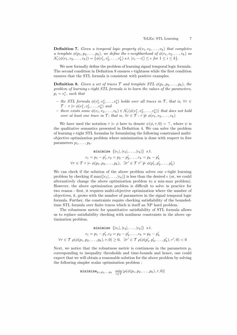
Definition 7. Given a temporal logic property φ(v1, v2, . . . , vk) that completesa template φ(p1, p2, . . . , pk), we define the ε-neighborhood of φ(v1, v2, . . . , vk) asNε(φ(v1, v2, . . . , vk)) = {φ(v′1, v

′2, . . . , v

′k) s.t. |vi − v′i| ≤ ε for 1 ≤ i ≤ k}.

We now formally define the problem of learning signal temporal logic formula.The second condition in Definition 8 ensures ε-tightness while the first conditionensures that the STL formula is consistent with positive examples.

Definition 8. Given a set of traces T and template STL φ(p1, p2, . . . , pk), theproblem of learning ε-tight STL formula is to learn the values of the parameters,pi = v∗i , such that

– the STL formula φ(v∗1 , v∗2 , . . . , v

∗k) holds over all traces in T , that is, ∀τ ∈

T : τ |= φ(v∗1 , v∗2 , . . . , v

∗k) and

– there exists some φ(v1, v2, . . . , vk) ∈ Nε(φ(v∗1 , v∗2 , . . . , v

∗k)) that does not hold

over at least one trace in T ; that is, ∃τ ∈ T : τ 6|= φ(v1, v2, . . . , vk)

We have used the notation τ |= φ here to denote ψ(φ, τ, 0) = >, where ψ isthe qualitative semantics presented in Definition 4. We can solve the problemof learning ε-tight STL formulas by formulating the following constrained multi-objective optimization problem where minimization is done with respect to freeparameters p1, . . . , pk.

minimize {|ε1|, |ε2|, . . . , |εk|} s.t.ε1 = p1 − p′1, ε2 = p2 − p′2, . . . , εk = pk − p′k

∀τ ∈ T τ |= φ(p1, p2, . . . , pk), ∃τ ′ ∈ T τ ′ 6|= φ(p′1, p′2, . . . , p

′k)

We can check if the solution of the above problem solves our ε-tight learningproblem by checking if max{|ε1|, . . . , |εk|} is less than the desired ε (or, we couldalternatively change the above optimization problem to a min-max problem).However, the above optimization problem is difficult to solve in practice fortwo reason - first, it requires multi-objective optimization where the number ofobjectives, k, grows with the number of parameters in the signal temporal logicformula. Further, the constraints require checking satisfiability of the bounded-time STL formula over finite traces which is itself an NP hard problem.

The robustness metric for quantitative satisfiability of STL formula allowsus to replace satisfiability checking with nonlinear constraints in the above op-timization problem.

minimize {|ε1|, |ε2|, . . . , |εk|} s.t.ε1 = p1 − p′1, ε2 = p2 − p′2, . . . , εk = pk − p′k

∀τ ∈ T ρ(φ(p1, p2, . . . , pk), τ, 0) ≥ 0, ∃τ ′ ∈ T ρ(φ(p′1, p′2, . . . , p

′k), τ ′, 0) < 0

Next, we notice that the robustness metric is continuous in the parameters picorresponding to inequality thresholds and time-bounds and hence, one couldexpect that we will obtain a reasonable solution for the above problem by solvingthe following simpler scalar optimization problem :

minimizep1,p2,...,pk minτ∈T|ρ(φ(p1, p2, . . . , pk), τ, 0)|

8 Jha, Tiwari, Seshia, Sahai and Shankar

87 9alpha

1

2

0

alpha8 97 alpha7 8 9

(a) (b) (c)

|R

obust

nes

s|

Idea

l M

etri

c

Tig

htn

ess

Met

ric

Fig. 1: (a) The absolute value of robustness metric reaches 0 at α = 8. It is closeto 0 even at 7.99 even though the temporal property corresponding to α = 7.99is violated by the trace. (b) The ideal metric should be negative when α < 8 andjump to ∞ when α = 8 and drop down to 0 when α > 8. (c) A metric which isnegative for α < 8, reaches its maxima between 8 and 8 + ε and then drops to 0.

There are two problems with this approach of solving the tight-STL learningproblem using the above optimization problem. This optimization problem usesthe absolute value of the robustness metric. This metric is generally not differ-entiable at ρ(φ(p1, p2, . . . , pk)) = 0. Further, if we get an ε-approximate solutionfor the above optimization problem, it no longer guarantees that all traces willsatisfy the instantiated template φ. This is because the absolute value can be asmall positive number even when the actual value is a small negative number.In Figure 1, we use the example at the beginning of the section to illustrate theproblem. Figure 1(b) illustrates an ideal metric, because it achieves its maximumat the the boundary of satisfiability and unsatisfiability. Maximizing this metricwould yield tight STL property but optimizing such a discontinuous function isdifficult. Figure 1(c) illustrates a more practical incarnation of the ideal metric,which is not discontinuous but still useful to learn ε tight STL property. Ourmain contribution is designing such a metric.

0 0.5

r = g( (t)) - = (Robustness Metric)-2

-1

0

1

2

3

4

5

Tig

htn

ess M

etr

ic

(r)

= 1

= 10

= 20

Fig. 2: Tightness metric θ for predicate

We begin by first defining a tightnessmetric for predicates. We would likethe metric to achieve its maximumvalue at the boundary in order to dis-cover tight STL properties. For a pred-icate µ(x) := g(x) ≥ α, recall thatthe robustness metric is ρ(µ, τ, t) =g(τ(t))−α = r. We would like to definea tightness metric θ(µ, τ, t) such that itis similar to Figure 1(c), and hence wedefine it to be

1

r + e−βr− e−r

TeLEx: STL Learning 9

where β ≥ 1 is an adjustable parame-ter. This function is plotted in Figure 2 and it approaches the ideal function inFigure 1(b) as β increases albeit at the cost of numerical stability during opti-mization. This function is smooth (its derivative is defined and also continuous),and hence, is amenable to gradient-based numerical optimization techniques.Finding an ε-tight value of α reduces to maximizing θ with appropriate choiceof β - lower values of ε require higher values of β.

0 100 200 300 400 500

Time interval t2 - t

1

0

500

1000

1500

2000

Tig

htn

ess M

etr

ic

= 0.01

= 0.015

(a) Globally Operator: θ(G[t2−t1]>)

0 100 200 300 400 500

Time interval t2 - t

1

0

0.2

0.4

0.6

0.8

1

Tig

htn

ess M

etr

ic

= 0.01

= 0.02

(b) Eventually Operator: θ(F[t2−t1]>)

Fig. 3: Tightness metric θ

Apart from the predicates, the other difficult cases for defining the tightnessmetric (θ) happen to be the temporal operators. The requirement here is that themetric θ should be defined such that it prefers longer time intervals for globallyoperator and shorter for eventually operator as illustrated in Figure 3.

We next formally define the tight quantitative semantics over negation-freeSTL properties and show how it can be used to formulate the problem of learningconsistent and tight STL property as a numerical optimization problem over asingle (scalar) cost metric. If the original formula has negation, it is pushedinwards through Boolean combinations, F and G temporal operations, and theinequality in predicate is flipped. Negation can also be pushed inwards throughdiscrete bounded time U operator via case-splitting. Further, since we deal withcontinuous signals, we consider only non-strict inequalities as predicates andrelax strict inequalities if needed.

Definition 9. The tightness metric θ : F × T × ST 7→ R ∪ {−∞,∞} maps anSTL formula φ ∈ F , a trace τ ∈ T , and a sampled time instance t ∈ ST to areal value s.t.:- θ(>, τ, t) =∞, θ(⊥, τ, t) = −∞- θ(µ, τ, t) = P(g(τ(t))− α) where µ(x) := (g(x) ≥ α)- θ(φ1 ∧ φ2, τ, t) = min(θ(φ1, τ, t), θ(φ2, τ, t))- θ(φ1 ∨ φ2, τ, t) = max(θ(φ1, τ, t), θ(φ2, τ, t))- θ(F[t1,t2]φ, τ, t) = C(γ, t1, t2) sup

t′∈[t+t1,t+t2]θ(φ, τ, t′)

- θ(G[t1,t2]φ, τ, t) = E(γ, t1, t2) inft′∈[t+t1,t+t2)

θ(φ, τ, t′)

- θ(φ1U[t1,t2]φ2, τ, t) = E(γ, t1, t2) supt′∈[t+t1,t+t2]

(min(θ(φ2, τ, t′), inf

t′′∈[t,t′)θ(φ1, τ, t

′′)))

10 Jha, Tiwari, Seshia, Sahai and Shankar

where the peak function P(r) = 1r+e−βr

− e−r,the contraction function C(γ, t1, t2) = 2

1+eγ(t2−t1+1) ,

the expansion function E(γ, t1, t2) = 21+e−γ(t2−t1+1) ,

β ≥ 1 is a coefficient chosen to determine sharpness of peak and γ ≥ 0 is acoefficient chosen to trade-off tightness in time vs tightness over predicates for agiven time-scale and spread of continuous variables. We choose to use the expan-sion function E in the definition of tightness of U-formulae. We could replace E

by C if shorter time-intervals are preferred in the U-operator.

If both the time-interval and predicate threshold is unknown for a temporaloperator, then there is a choice in either tightening time-intervals and discoveringpredicates that hold over these or to find tighter predicates over longer (in caseof eventually) and shorter (in case of globally) operators. Increasing γ wouldresult in tighter time-intervals. Increasing β would result in tighter predicates. Inthe following theorem, we summarize the relation between the tightness metricand satisfaction of STL formula.

Theorem 1. The tightness metric for a given STL formula φ, namely θ(φ, τ, t)is nonnegative if and only if τ satisfies φ at time t.

Proof. We first show that θ(φ, τ, t) ≥ 0 if and only if ρ(φ, τ, t) ≥ 0 using struc-tural induction. We have only two nontrivial cases:- Atomic Predicates: We know that 1

r+e−βr− e−r ≥ 0 where β ≥ 1 if and only

if r ≥ 0. Hence, θ(µ, τ, t) = 1r+e−βr

− e−r ≥ 0 if and only if r = g(τ(t)) − α =ρ(µ, τ, t) ≥ 0- Temporal Operators: C(γ, t1, t2) = 2

1+eγ(t2−t1+1) ≥ 0 for all t2 > t1 and

E(γ, t1, t2) = 21+e−γ(t2−t1+1) ≥ 0 for all t2 > t1. Hence, θ has the same sign

as ρ, that is, θ(φ, τ, t) ≥ 0 if and only if ρ(φ, τ, t) ≥ 0.Thus, θ(φ, τ, t) ≥ 0 if and only if ρ(φ, τ, t) ≥ 0 and we know that ρ(φ, τ, t) ≥ 0 ifand only if τ satisfies φ at time t. ut

The theorem above shows that a STL formula φ that has positive tightnessmetric (over all the traces τ in some set T ) will also evaluate to True in allthese traces. But we want a formula that is not only consistent with the traces,but also tight on the traces. The following lemma says that optimizing for thetightness metric results in tight formulas.

Lemma 1. Given a trace τ and a template STL formula φ(p1, p2, . . . , pk) withk unknown parameters (Definition 6), let

(v∗1 , v∗2 , . . . , v

∗k) = arg max

p1,p2,...,pkθ(φ(p1, p2, . . . , pk), τ, 0)

be a solution v∗ = (v∗1 , . . . , v∗k) such that θ(φ(v∗), τ, 0) is a finite nonnegative

value. Then v∗ is a solution for the ε-tight STL learning problem on the singletonset {τ} of traces for any value of ε such that ε > η, where η is no more than therobustness ρ(φ(v∗), τ, 0) of the discovered instantated formula. The value η canbe made arbitrarily small with appropriate choice of β, γ.

TeLEx: STL Learning 11

Proof. (Sketch) We again argue by structural induction over the template φ.Since φ is negation-free, we have three cases. (Case 1) If the top symbol of φis a temporal operator with a time bound [t1, t2] such that either t1 or t2 is aparameter, then our definition of θ guarantees that the interval [t∗1, t

∗2] (in the

instantiated solution) is maximally elongated or contracted, and hence φ(v∗)can be falsified by an ε perturbatation to the interval, for any ε > 0. (Case 2)If φ is an atomic predicate, then the robustness measure ρ clearly defines theminimum perturbation required to falsify it. (Case 3) If the top symbol of φ is∨ or ∧, we can reason inductively one or both of the subformulas.

For the second part, note that we can decrease η by choosing a large βand γ > 0. (Case 1) The value of r at which the function 1

r+e−βr− e−r peaks

monotonically decreases with β and hence, more tight predicates (smaller r) canbe learnt by increasing β. Hence, η decreases by increasing β. (Case 2) From thedefinition of C, we observe that the function 2

1+eγ(∆t+1) decreases monotonically

with γ and the function 21+e−γ(∆t+1) increases monotonically with γ. Thus, if γ >

0, these functions cause us to learn the largest or smallest possible time interval,and hence changing the learnt intervals even slightly falsifies the formula. Hence,if γ > 0, then η = 0 for formulas that have a parametric temporal operator atthe top. ut

We can lift Lemma 1 to a set of traces, but we lose the ability to arbitrarilydecrease η.

Theorem 2. Given a set of traces T and a template STL formula φ(p1, p2, . . . , pk),let

(v∗1 , v∗2 , . . . , v

∗k) = arg max

p1,p2,...,pk[minτ∈T

θ(φ(p1, p2, . . . , pk), τ, 0)]

define the solution v∗ = (v∗1 , . . . , v∗k) such that minτ∈T θ(φ(v∗), τ, 0) is nonnega-

tive. Then the learnt formula φ(v∗) solves the ε-tight STL learning problem fora value of ε such that ε > η, where η = minτ∈T ρ(φ(v∗1 , . . . , v

∗k), τ, 0) is the stan-

dard robustness measure of the discovered instantated formula. The value η getsno larger by increasing β and γ.

We use an off-the-shelf solver - quasi-Newton algorithm [12, 34] to solve theabove optimization problem. It uses gradient during optimization where thesearch direction in each iteration i is computed as di = −Higi. Hi is the inverseof the Hessian matrix and gi is the current derivative. The Hessian is a matrix ofsecond-order partial derivatives of the cost function and describes its local cur-vature. Due to the smoothness of the defined tightness metric θ, gradient-basedoptimization techniques are very effective in solving the STL learning problemsince both the gradient and the Hessian can be conveniently computed. We alsoused the gradient-free optimization to experimentally validate the advantage ofsmoothness of tightness metric. The optimization engine behind gradient-freeoptimization is differential evolution [29].

12 Jha, Tiwari, Seshia, Sahai and Shankar

5 Experimental Evaluation

The presented approach is implemented in a publicly available tool: TeLEx4.We evaluated the effectiveness of TeLEx on a number of synthetic and real case-studies. All experiments were conducted on a quad core Intel Core i5-2450MCPU @ 2.50GHz with 3MB cache per core and 4 GB RAM.

1. Temporal Bounds on Signal x(t) = t sin(t2)

This case-study was designed to evaluate the scalability of TeLEx as well asthe tightness of learnt STL formulae using a synthetic trajectory for which wealready know the correct answer. We also compare gradient-based TeLEx withgradient-free optimization to demonstrate the utility of smoothness of proposedtightness metric. We consider the signal x(t) = t sin(t2). We consider 12 STLtemplates of the form:

template(k) ≡k∧i=0

(G[i,i+1](x ≤ p2i ∧ x ≥ p2i+1))

where k = 0, 1, . . . , 11. Thus, the number of parameters in these templates growfrom 2 to 24. We repeated learning experiments 10 times in each case sincenumerical optimization routines are not deterministic.

-15

-10

-5

0

5

10

15

0 2 4 6 8 10 12

x(t

) and learn

t bounds

time t (seconds)

x(t)

(a) x(t) and learned bounds

0

20

40

60

80

100

120

0 5 10 15 20 25

Runtim

e (

seconds)

Number of Parameters

gradient-based

(b) Gradient-based runtime

0

500

1000

1500

2000

2500

3000

3500

0 5 10 15 20

Runtim

e (

seconds)

Number of Parameters

gradient-free

(c) Gradient-free runtime

Fig. 4: Tightness and Scalability of TeLEx Using Gradient Based Optimization

Figure 4(a) shows the signal trace from time t = 0 to t = 12 along with thebounds discovered by TeLEx while synthesizing the STL property using tem-plate template(12) (the largest template) and gradient-based optimization. Thetightness of bounds demonstrates that the learnt STL properties are tight (andhave very low variance) even with 24 parameters. The robustness values forlearnt STL properties were always very small (between 0.02 and 0.12). We ob-served that gradient-free differential evolution also discovered tight propertiesin all cases (robustness value between (0.06 and 0.35) in which it terminated.Figure 4(b) and (c) show the runtime of gradient-based and gradient-free opti-

4 https://github.com/susmitjha/TeLEX

TeLEx: STL Learning 13

mization techniques respectively. Gradient-free methods did not terminate in anhour for more than 18 parameters. We plot the mean runtime (along with stan-dard deviation) from 10 runs with respect to the number of parameters beinglearnt for each of the 12 templates. The variability in runtime (standard devia-tion plotted as error bars) increases with the number of parameters. We observea speed-up of 30X-100X using gradient-based approach due to the smoothnessof tightness metric (scales of y-axis in Figure 4(b) and (c) are different).

2. Two Agent Surveillance

0,0 5,0 10,0

0,5

0,10 5,10 10,10

10,5

Fig. 5: Two Agent Surveil-lance

We consider a two agent surveillance system inwhich both agents monitor a 10x10 grid as illus-trated in Figure 5. Intruders can pop up at any ofthe 8 locations marked by circles. But at any point,there are at most two intruders. The two agents areinitially at 0, 0 and 10, 10 respectively. The agentsfollow a simple protocol. At each time-instant, theagents calculate the distance from their current lo-cation to the intruders (if any), then they select theintruder closest to them as their target for inspec-tion and move towards it. The target of an agentmight change while moving (when second intruderpops up and it is closer to the agent moving to-wards first). After an intruder location is inspected,it is considered neutralized and the agent stays thereuntil new target emerges. The simulator for this simple surveillance protocol isavailable at the tool website5. We simulated this for 1000 time-steps and thenused TeLEx to learn STL corresponding to the following two properties.

– The maximum time between intruder popping up and being neutralized is39.001 time-steps.

– The distance between the two agents is at least 4.998. This non-collisionbetween agents is an emergent property due to “move-to-closest” policy ofagents and the fact that there are at most two intruders at any given time.

2. Udacity Autonomous-Car Driving Public Data-set

In this case-study, we use the data made available publicly by Udacity as apart of its second challenge for autonomous driving6. The data corresponds toan instrumented car (2016 Lincoln MKZ) driving along El Camino Real (a majorroad in San Francisco Bay Area) starting from the Udacity office in MountainView and moving north towards San Francisco. We use HMB 1 data-set whichis a 221 seconds snippet with a total of over 13205 samples. It has a mixture ofturns and straight driving. The data-set includes steering angle, applied torque,

5 https://github.com/susmitjha/TeLEX/blob/master/tests/twoagent.py6 https://github.com/udacity/self-driving-car/tree/master/challenges/challenge-2

14 Jha, Tiwari, Seshia, Sahai and Shankar

speed, throttle, brake, GPS and image. For our purpose, we focus on non-imagedata. The goal of this data-set is to provide real-world training sample for au-tonomous driving. Figure 6 shows how the angle and speed vary in the Udacitydata-set.

(a) Angle (b) Speed

Fig. 6: Angle and Speed for a subset of Udacity data

We use the tight STL learning approach presented in this paper to learntemporal properties relating angle, torque and speed. Such learned temporalproperties could have several utilities. It could be used to examine whether adriving pattern (autonomous or manual) is too conservative or too risky. It couldbe used to extract sensible logical relations that must hold between differentcontrol inputs (say, speed and angle) from good manual driving data, and thenenforce these temporal properties on autonomous driving systems. It could alsobe used to compare different autonomous driving solutions. We are interestedin the following set of properties and we present the result of extracting theseusing TeLEx . We would like the robustness metric to be as close to 0 as possibleand in all experiments below, we found it to be below 0.005.

1. The speed of the car must be below some upper bound a ∈ [15, 25] if theangle is larger than 0.2 or below -0.2. Intuitively, this property capturesrequired slowing down of the car when making a significant turn.

Template STL: G[0, 2.2e11](((angle ≥ 0.2)|(angle ≤ −0.2))⇒ (speed ≤ a?15; 25))

Synthesized STL: G[0.0, 2.2e11](((angle ≥ 0.2)|(angle ≤ −0.2))⇒ (speed ≤ 22.01))

Performance: Tightness Metric = 0.067, Robustness Metric = 0.004Runtime: 8.64 seconds

2. Similar to the property above, the speed of the car must be low while ap-plying a large torque (say, more than 1.6). Usually, torque is applied to turnalong with brake when driving safely to avoid slipping.

Template STL: G[0, 2.2e11](((torque ≥ 1.6)|(torque ≤ −1.6))⇒ (speed ≤ a?15; 25))

Synthesized STL: G[0.0, 2.2e11](((torque ≥ 1.6)|(torque ≤ −1.6))⇒ (speed ≤ 23.64))

Performance: Tightness Metric = 0.221, Robustness Metric = 0.005Runtime: 10.12 seconds

TeLEx: STL Learning 15

3. Another property of interest is to ensure that when the turn angle is high(say, above 0.06), the magnitude of negative torque applied is below a thresh-old. This avoids unsafe driving behavior of making late sharp compensationtorques to avoid wide turns.

Template STL: G[0, 2.2e11]((angle ≥ 0.06)⇒ (torque ≥ b?− 2;−0.5))

Synthesized STL: G[0.0, 2.2e11]((angle ≥ 0.06)⇒ (torque ≥ −1.06))

Performance: Tightness Metric = 0.113, Robustness Metric = 0.003Runtime: 7.30 seconds

4. Similarly, when the turn angle is low (say, below -0.06), the magnitude ofpositive torque applied is below a threshold to avoid late sharp compensatingtorques.

Template STL: G[0, 2.2e11]((angle ≤ −0.06)⇒ (torque ≤ b?0.5; 2))

Synthesized STL: G[0.0, 2.2e11]((angle ≤ −0.06)⇒ (torque ≤ 1.25))

Performance: Tightness Metric = 0.472, Robustness Metric = 0.002Runtime: 5.00 seconds

5. The torque also must not be so low that the turns are very slow and so, werequire that application of negative torque should decrease the angle belowa threshold within some fixed time.

Template STL: G[0, 2.2e11]((torque ≤ 0.0)⇒ F [0.0, 1.2e8](angle ≤ a?− 1; 1))

Synthesized STL: G[0.0, 2.2e11]((torque ≤ 0.0)⇒ F [0.0, 1.2e8](angle ≤ 0.01))

Performance: Tightness Metric = 0.727, Robustness Metric = 0.002Runtime: 46.59 seconds

6 Conclusion

In this paper, we presented a novel approach to learn tight STL formula usingonly positive examples. Our approach is based on a new tightness metric thatuses smooth functions. The problem of learning tight STL properties admitsa number of pareto-optimal solutions. We would like to add the capability ofspecifying preference in which parameters are tightened. Further, computationof the metrics on traces over optimization can be easily parallelized. Another di-mension is to study other metrics proposed in literature to quantify conformanceand extend tightness over these metrics [8, 19]. In conclusion, TeLEx automatesthe learning of high-level STL properties from observed time-traces given user-guidance in form of templates. It relies on a novel tightness metric defined in thispaper which is smooth and amenable to gradient-based numerical optimizationtechniques.

AcknowledgementThis work is supported in part by DARPA under contract FA8750-16-C-0043and NSF grant CNS-1423298.

16 Jha, Tiwari, Seshia, Sahai and Shankar

References

1. Abbas, H., Hoxha, B., Fainekos, G., Ueda, K.: Robustness-guided temporal logictesting and verification for stochastic cyber-physical systems. In: Cyber Technologyin Automation, Control, and Intelligent Systems (CYBER), 2014 IEEE 4th AnnualInternational Conference on. pp. 1–6. IEEE (2014)

2. Abbas, H., Winn, A., Fainekos, G., Julius, A.A.: Functional gradient descentmethod for metric temporal logic specifications. In: American Control Conference(ACC), 2014. pp. 2312–2317. IEEE (2014)

3. Akazaki, T.: Falsification of conditional safety properties for cyber-physical sys-tems with gaussian process regression. In: International Conference on RuntimeVerification. pp. 439–446. Springer (2016)

4. Aksaray, D., Jones, A., Kong, Z., Schwager, M., Belta, C.: Q-learning for robustsatisfaction of signal temporal logic specifications. In: Decision and Control (CDC),2016 IEEE 55th Conference on. pp. 6565–6570. IEEE (2016)

5. Angluin, D.: Identifying languages from stochastic examples. Tech. rep.,YALEU/DCS/RR-614, Yale University. Department of Computer Science (1988)

6. Annpureddy, Y., Liu, C., Fainekos, G., Sankaranarayanan, S.: S-taliro: A tool fortemporal logic falsification for hybrid systems. In: International Conference onTools and Algorithms for the Construction and Analysis of Systems. pp. 254–257.Springer (2011)

7. Bartocci, E., Bortolussi, L., Sanguinetti, G.: Data-driven statistical learning oftemporal logic properties. In: International Conference on Formal Modeling andAnalysis of Timed Systems. pp. 23–37. Springer (2014)

8. Deshmukh, J.V., Majumdar, R., Prabhu, V.S.: Quantifying conformance using theskorokhod metric. In: International Conference on Computer Aided Verification.pp. 234–250. Springer (2015)

9. Donze, A.: Breach, a toolbox for verification and parameter synthesis of hybridsystems. In: International Conference on Computer Aided Verification. pp. 167–170. Springer (2010)

10. Donze, A.: On signal temporal logic. In: International Conference on RuntimeVerification. pp. 382–383. Springer (2013)

11. Donze, A., Maler, O.: Robust satisfaction of temporal logic over real-valued signals.In: International Conference on Formal Modeling and Analysis of Timed Systems.pp. 92–106. Springer (2010)

12. Facchinei, F., Lucidi, S., Palagi, L.: A truncated newton algorithm for large scalebox constrained optimization. SIAM Journal on Optimization 12(4), 1100–1125(2002)

13. Fainekos, G.E., Pappas, G.J.: Robustness of temporal logic specifications. In:Formal Approaches to Software Testing and Runtime Verification, pp. 178–192.Springer (2006)

14. Fu, J., Topcu, U.: Synthesis of joint control and active sensing strategies under tem-poral logic constraints. IEEE Trans. Automat. Contr. 61(11), 3464–3476 (2016),http://dx.doi.org/10.1109/TAC.2016.2518639

15. Giuseppe, B., Cristian Ioan, V., Francisco, P.A., Hirotoshi, Y., Calin, B.: A DecisionTree Approach to Data Classification using Signal Temporal Logic. In: HybridSystems: Computation and Control (HSCC). pp. 1–10. Vienna, Austria (April2016)

16. Gold, E.M.: Language identification in the limit. Information and control 10(5),447–474 (1967)

TeLEx: STL Learning 17

17. Horning, J.J.: A study of grammatical inference. Tech. rep., DTIC Document(1969)

18. Hoxha, B., Dokhanchi, A., Fainekos, G.: Mining parametric temporal logicproperties in model based design for cyber-physical systems. arXiv preprintarXiv:1512.07956 (2015)

19. Jaksic, S., Bartocci, E., Grosu, R., Nickovic, D.: Quantitative monitoring of stl withedit distance. In: International Conference on Runtime Verification. pp. 201–218.Springer (2016)

20. Jha, S., Raman, V.: Automated synthesis of safe autonomous vehicle control underperception uncertainty. In: Rayadurgam, S., Tkachuk, O. (eds.) NASA FormalMethods: 8th International Symposium, NFM. pp. 117–132 (2016)

21. Jha, S., Raman, V.: On optimal control of stochastic linear hybrid systems. In:Franzle, M., Markey, N. (eds.) Formal Modeling and Analysis of Timed Systems:14th International Conference, FORMATS. pp. 69–84. Springer International Pub-lishing (2016), http://dx.doi.org/10.1007/978-3-319-44878-7_5

22. Jha, S., Seshia, S.A.: A theory of formal synthesis via inductive learning. ActaInformatica (Feb 2017), https://doi.org/10.1007/s00236-017-0294-5

23. Jin, X., Donze, A., Deshmukh, J.V., Seshia, S.A.: Mining requirements from closed-loop control models. IEEE Transactions on Computer-Aided Design of IntegratedCircuits and Systems 34(11), 1704–1717 (2015)

24. Kong, Z., Jones, A., Medina Ayala, A., Aydin Gol, E., Belta, C.: Temporal logicinference for classification and prediction from data. In: Proceedings of the 17thinternational conference on Hybrid systems: computation and control. pp. 273–282.ACM (2014)

25. Lindemann, L., Dimarogonas, D.V.: Robust control for signal temporal logic spec-ifications using average space robustness. arXiv preprint arXiv:1607.07019 (2016)

26. Maler, O., Nickovic, D.: Monitoring temporal properties of continuous signals. In:Formal Techniques, Modelling and Analysis of Timed and Fault-Tolerant Systems,pp. 152–166. Springer (2004)

27. Maler, O., Nickovic, D., Pnueli, A.: Checking temporal properties of discrete, timedand continuous behaviors. In: Pillars of computer science, pp. 475–505. Springer(2008)

28. Muggleton, S.: Learning from positive data, pp. 358–376. Springer Berlin Heidel-berg, Berlin, Heidelberg (1997)

29. Price, K., Storn, R.M., Lampinen, J.A.: Differential evolution: a practical approachto global optimization. Springer Science & Business Media (2006)

30. Raman, V., Donze, A., Maasoumy, M., Murray, R.M., Sangiovanni-Vincentelli,A.L., Seshia, S.A.: Model predictive control with signal temporal logic specifica-tions. In: CDC. pp. 81–87 (Dec 2014)

31. Sadraddini, S., Belta, C.: Robust temporal logic model predictive control. In: Com-munication, Control, and Computing (Allerton), 2015 53rd Annual Allerton Con-ference on. pp. 772–779. IEEE (2015)

32. Valiant, L.G.: A theory of the learnable. Communications of the ACM 27(11),1134–1142 (1984)

33. Yang, H., Hoxha, B., Fainekos, G.: Querying parametric temporal logic propertieson embedded systems. In: IFIP International Conference on Testing Software andSystems. pp. 136–151. Springer (2012)

34. Zhu, C., Byrd, R.H., Lu, P., Nocedal, J.: Algorithm 778:fortran subroutines forlarge-scale bound-constrained optimization. ACM Transactions on MathematicalSoftware (TOMS) 23(4), 550–560 (1997)