Temi di discussione(Working Papers)

Expansionary yet different: credit supply and real effects of negative interest rate policy

by Margherita Bottero, Camelia Minoiu, José-Luis Peydró, Andrea Polo, Andrea F. Presbitero and Enrico Sette

Num

ber 1269M

arch

202

0

Temi di discussione(Working Papers)

Expansionary yet different: credit supply and real effects of negative interest rate policy

by Margherita Bottero, Camelia Minoiu, José-Luis Peydró, Andrea Polo, Andrea F. Presbitero and Enrico Sette

Number 1269 - March 2020

The papers published in the Temi di discussione series describe preliminary results and are made available to the public to encourage discussion and elicit comments.

The views expressed in the articles are those of the authors and do not involve the responsibility of the Bank.

Editorial Board: Federico Cingano, Marianna Riggi, Monica Andini, Audinga Baltrunaite, Marco Bottone, Davide Delle Monache, Sara Formai, Francesco Franceschi, Salvatore Lo Bello, Juho Taneli Makinen, Luca Metelli, Mario Pietrunti, Marco Savegnago.Editorial Assistants: Alessandra Giammarco, Roberto Marano.

ISSN 1594-7939 (print)ISSN 2281-3950 (online)

Printed by the Printing and Publishing Division of the Bank of Italy

EXPANSIONARY YET DIFFERENT: CREDIT SUPPLY AND REAL EFFECTS OF NEGATIVE INTEREST RATE POLICY

by Margherita Bottero*, Camelia Minoiu^, José-Luis Peydró§, Andrea Polo~, Andrea F. Presbitero° and Enrico Sette*

Abstract We show that negative interest rate policy (NIRP) has expansionary effects on bank

credit supply - and the real economy - through a portfolio rebalancing channel, and that, by shifting down and flattening the yield curve, NIRP differs from rate cuts just above the zero lower bound. For identification, we exploit ECB’s NIRP and matched administrative datasets - including the credit register - from Italy, severely hit by the Eurozone crisis. NIRP affectsbanks with higher ex-ante net short-term interbank positions or, more broadly, more liquidbalance-sheets. NIRP-affected banks rebalance their portfolios from liquid assets to lending,especially to ex-ante riskier and smaller firms - without higher ex-post delinquencies - and cutloan rates (even to the same firm), inducing sizable firm-level real effects. By contrast, thereis no evidence of a retail deposits channel associated with NIRP.

JEL Classification: E52, E58, G01, G21, G28. Keywords: negative interest rates, portfolio rebalancing, bank lending channel of monetary policy, liquidity management, Eurozone crisis. DOI: 10.32057/0.TD.2020.1269

Contents

1. Introduction ......................................................................................................................... 5 2. Institutional background .................................................................................................... 14 3. Data and empirical hypotheses .......................................................................................... 16

3.1 The credit register and other data ............................................................................... 16 3.2 Identification strategy ................................................................................................. 18 3.3 Empirical specifications ............................................................................................. 21

4. Credit supply ..................................................................................................................... 24 4.1 Main results ................................................................................................................ 24 4.2 Robustness of the baseline .......................................................................................... 26 4.3 NIRP vs. other monetary policy events ...................................................................... 28 4.4 Falsification tests ....................................................................................................... 30 4.5 NIRP and portfolio rebalancing across Euro area banks ........................................... 31 4.6 Heterogeneity: firm risk and size .............................................................................. 32 4.7 Transmission to loan rates ......................................................................................... 33

5. Real effects ....................................................................................................................... 34 6. Conclusions ....................................................................................................................... 35 References .............................................................................................................................. 37 Figures and tables .................................................................................................................. 42 Online appendix ..................................................................................................................... 52 _______________________________________ * Bank of Italy, Directorate General for Economics, Statistics and Research - Economic Research and

International Relations.^ Federal Reserve Board. § ICREA-UPF, Barcelona GSE, CREI, CEPR, Imperial College London.~ LUISS, UPF, Barcelona GSE, EIEF, CEPR, ECGI.° International Monetary Fund and MoFiR.

“Negative [policy] rates were introduced for one specific reason: when interest rates reached thezero lower bound, the expectations for the future rates in the long term are only that the rates can

go up. So with negative rates we were successful in taking these expectations down“

“By and large our negative interest-rate policies have been a success. [. . . ] We haven’t seen bankprofitability going down; in fact it is going up.”

Mario Draghi (2016, 2017), President of the European Central Bank

1 Introduction1

Negative nominal interest rates are a significant innovation in monetary policy-making, with impor-

tant implications for finance and macroeconomics. Long thought as unrealistic, negative interest rate

policy (NIRP) was recently adopted in several advanced economies by paying negative rates on bank

deposits at central banks. The first central bank to do so was the Danish National Bank in 2012, fol-

lowed by the European Central Bank (ECB), the Swiss National Bank, the Sveriges Riksbank, and the

Bank of Japan. NIRP may become even more important given that current interest rates are low and

central banks may need to further cut rates.2 Moreover, from a theoretical point of view, the effects

of NIRP on the economy are a priori unclear. While negative rates may boost aggregate demand by

removing the zero lower bound (ZLB) (Bernanke, 2017; Rogoff, 2016, 2017), they could also be con-

tractionary through bank lending (Brunnermeier and Koby, 2018; Eggertsson et al., 2019). Despite

the importance of NIRP for the broader understanding of finance and macroeconomics, systematic

evidence on its transmission to the economy through the banking system remains scarce.

The introduction of NIRP as an unconventional tool of monetary policy raises two major ques-

tions. First, what is the impact of this policy on credit supply and the real economy? Second, do

negative monetary policy rates differ in their transmission to the economy from conventional rate

cuts just above the ZLB, and from other unconventional monetary policies, such as quantitative eas-

ing (QE)? In this paper, we answer these questions by exploiting the ECB’s introduction of negative

1We thank David Arseneau, Gabriel Chodorow-Reich, Vitor Costancio, Giovanni Dell’Ariccia, Davide Fantino, DimasMateus Fazio, Xavier Freixas, Luca Fornaro, Michael Gofman, Charles, Goodhart, Lucyna Gornicka, Yuriy Gorodnichenko,Luca Guerrieri, Florian Heider, Tumer Kapan, Kebin Ma, David Martinez Miera, Emi Nakamura, Marco Pagano, DanielParavisini, Rafael Repullo, Ken Rogoff, Kasper Roszbach, Marcelo Ulate, William White, and participants at the 2019 NBERSummer Institute (Monetary Economics) and numerous conferences and seminars for useful comments and discussions.Camelia Minoiu is grateful to the Wharton Financial Institutions Center and the Management Department at the Universityof Pennsylvania for their hosting during the development of this research project. This project has received funding fromthe European Research Council (ERC) under the European Union’s Horizon 2020 research and innovation programme(grant agreement No 648398). Peydró also acknowledges financial support from the ECO2015-68182-P (MINECO/FEDER,UE) grant and the Spanish Ministry of Economy and Competitiveness, through the Severo Ochoa Programme for Centresof Excellence in R&D (SEV-2015-0563). The views expressed herein are those of the authors and should not be attributed tothe Bank of Italy, the Federal Reserve Board, the IMF, their management, or policies.

2Since 1970 policy rates have been cut by more than 500 basis points in response to recessions in the U.S. and theeuro area (Eggertsson et al., 2019). Moreover, in 2019 both the US and euro area (as well as many other countries) havesignificantly cut monetary policy rates (in parallel with downward revisions in GDP growth forecasts).

5

nominal policy rates in mid-2014 (as well as other policy rate cuts) and Italian administrative data on

loan volumes and lending rates from the credit register, matched with firm- and bank-level balance

sheet data. As part of a monetary union, Italy provides an excellent setting to study NIRP in the

context of contracting GDP in 2012 and 2013, while the ECB’s balance sheet was shrinking and euro

area monetary conditions were tighter than in several other countries.

In brief, we find an increase in total bank credit growth after the introduction of NIRP using

aggregate time-series data. The announcement of NIRP shifted down and flattened the risk-free

yield curve, widening the spread between the yields of safer, liquid assets and those of corporate

loans. Thus, we find that NIRP affected relatively more those banks with higher ex-ante net short-

term interbank positions (as short-term interbank rates became negative) or, more broadly, those

banks with more liquid balance-sheets (since the change in the yield curve affected all maturities).

A loan-level analysis shows that more NIRP-affected banks cut liquid assets and expand credit

supply more, in particular to ex-ante riskier and smaller firms—without higher ex-post non-perform-

ing loans (NPLs)—and cut loan rates, inducing sizable firm-level real effects. Our evidence is incon-

sistent with the view that banks that rely more on retail deposits change (reduce) the supply of credit

volumes, or loan rates, in response to NIRP; instead, we show that banks preserve margins and

profitability, also by raising fees on bank deposits. Moreover, previous monetary policy rate cuts in

positive territory close to the ZLB were unable to flatten the yield curve and did not cause a simi-

lar rebalancing of bank portfolios; differently from the announcements of QE in January 2015 and

the most recent policy negative rate cut in March 2016, both of which were associated with further

flattening of the yield curve and portfolio rebalancing.3

Our main contribution to the literature is to document that NIPR has expansionary effects, and yet

differs from rate cuts just above the ZLB. The mechanism at work is via shifting down and flattening

the yield curve, and hence incentivizing banks to rebalance their portfolio from liquid assets to credit

supply. Furthermore, we show that the bank lending channel of NIRP is different from the traditional

channel associated with interest rate cuts above the ZLB (Kashyap and Stein, 1995, 2000; Jiménez

et al., 2012; Drechsler et al., 2017). We find no evidence of a retail deposits channel (unlike Eggertsson

et al. (2019) and Heider et al. (2019)), even after the last rate cut.4 Below, we provide a detailed

3In September 2019 the ECB further reduced the negative rate, but data to analyze this additional cut are not yet avail-able. The ECB also changed the implementation of the policy by introducing a two-tier system for reserve remuneration,exempting parts of banks’ liquidity holdings from negative remuneration.

4The results on the portfolio rebalancing and the retail deposits channels are not specific to the Italian context, as theyare confirmed by a bank-level analysis for the entire euro area.

6

preview of the paper and discuss the novelty of our findings in relation to the literature.

Detailed preview of the paper. Macroeconomic theory argues that a policy rate cut expands ag-

gregate demand (thereby boosting economic growth and prices), hence it finds in the ZLB an im-

portant constraint in a situation of adverse economic conditions (Bernanke, 2017; Rogoff, 2016, 2017;

Dell’Ariccia et al., 2018). As shown in the opening quotes, Draghi (2017) argues that NIRP has had

positive effects. However, other central banks, including the U.S. Federal Reserve and the Bank of

England, have been less keen to adopt this policy (Bernanke, 2016).5 One reason is that the positive

aggregate demand channel could be offset by a contraction in credit supply due to the adverse effect

of NIRP on banks’ net worth (Eggertsson et al., 2019; Sims and Wu, 2019; Ulate, 2019). Brunnermeier

and Koby (2018) theoretically show that there may be a “reversal” interest rate beyond which lower

rates undo the cut’s intended effects on bank lending and become contractionary. This reversal rate is

a low interest rate, potentially even negative. Very low interest rates are also believed to drive finan-

cial intermediary reach-for-yield behavior (Rajan, 2005; Taylor, 2009; Allen and Rogoff, 2011; Stein,

2013; Martinez-Miera and Repullo, 2017), consistent with a risk-taking channel of monetary policy

(Adrian and Shin, 2010; Borio and Zhu, 2012).

Negative policy rates can affect the real economy through the banking system primarily through

two, non-mutually exclusive, channels. A first channel of transmission hinges on the pass-through

of negative policy rates to bank retail deposit rates (“retail deposits channel”). Given that banks are

generally reluctant to charge negative rates on retail deposits, NIRP may reduce banks’ net interest

margins and profits, eroding their capital and reducing their lending capacity. This phenomenon

should be more pronounced for banks that are more dependent on retail deposits, leading them to

curtail credit and take more risk (Heider et al., 2019) or/and to weaken the pass-through to loan

rates (Eggertsson et al., 2019). By contrast, other studies argue that the contractionary effects of NIRP

could be relatively small. Ulate (2019), for instance, calibrates a DSGE model with monopolistic com-

petition in the banking sector to show that the adverse effect of negative rates on bank profitability

is dampened by the increase in aggregate demand, which allows banks to switch from reserves to

loans. In addition, the monetary transmission mechanisms would not be impaired if banks passed

5Bernanke (2016) on the views of the Federal Reserve’s decision body (Federal Open Market Committee, FOMC) andthe Bank of England regarding NIRP: “Interestingly, some advocates of a higher inflation target have been dismissive of the use ofnegative short-term interest rates, an alternative means of increasing “space” for monetary easing [. . . ] Williams said: “Negative ratesare still at the bottom of the stack in terms of net effectiveness.” Williams’s colleague on the FOMC, Eric Rosengren, has suggestedthat [. . . ] negative rates should be viewed as a last resort. My sense is that Williams’s and Rosengren’s negative view of negative ratesis broadly shared on the FOMC. Outside the United States, Mark Carney, governor of the Bank of England [. . . ] has indicated he was“not a fan” of negative interest rates.”

7

negative rates to some retail depositors—as shown for a set of sound European banks by Altavilla

et al. (2019)—or if banks with large retail deposits simultaneously charged higher fees to preserve

profitability (Altavilla et al., 2018; IMF, 2016; Lopez et al., 2018).

An alternative transmission channel works through portfolio rebalancing actions by banks with

safer, more liquid assets. Negative interest rates penalize the holdings of such assets, incentivizing

banks to shift their portfolios away from low- or negative-yield liquid assets towards higher-yield

assets such as corporate loans (a “portfolio rebalancing channel”, see e.g., Bernanke (2016); Rostagno

et al. (2016)). In the words of Brunnermeier and Koby (2018): "as yields on safe assets decrease, banks

decrease their lending rates for risky loans in order to substitute their safe assets positions into riskier high-

yield ones, another effect which the central bank seeks to induce." This would be especially the case if NIRP

moves the entire yield curve downward—after breaking through the ZLB, market participants may

expect rates to stay low or negative for long (see Draghi’s 2016 initial quote). The fall in the yield

of safer assets of all maturities would widen the wedge between safer, more liquid and riskier, more

illiquid assets, and may lead banks to rebalance their portfolio to preserve profitability. According

to this logic, a policy rate cut into negative territory would work differently from regular policy rate

cuts (in positive territory) in the proximity of the ZLB, but similarly to QE given the accompanying

flattening of the yield curve,6 and increase in the safety premium (see Krishnamurthy and Vissing-

Jorgensen (2011) for the U.S.). Furthermore, portfolio rebalancing toward loans can additionally be

incentivized by a reduction in the risk of corporate loans. The announcements of NIRP, or of QE, are

large monetary policy shocks—they flatten the yield curve—so they are able to promote recovery in

the real economy, thereby raising corporate profits and reducing corporate delinquency and default

rates (Chodorow-Reich, 2014).

Italy provides an ideal set-up for the analysis of NIRP because of its administrative datasets and

specific context. We use the supervisory credit register of the Bank of Italy, which offers detailed

information on bank loans to all Italian firms, and from which we obtain outstanding loan volumes

and lending rates at the firm-bank-month level. This is a major data advantage as loan rates are ab-

sent in most the credit registers around the world. We double-match this dataset with detailed firm

and bank balance sheet information to study the effects of NIRP on both firms and banks that are

connected through credit relationships. Data on bank balance sheets come from supervisory reports,

while data on firm financials are obtained from the official balance sheet data deposited by firms to

the Chambers of Commerce, as required by Italian law. These datasets allow us to conduct a compre-

6See, e.g. Gambetti and Musso (2017); Altavilla et al. (2015) for the euro area; D‘Amico and King (2013) for the U.S.

8

hensive analysis of bank asset allocations and their spillovers to the real economy when policy rates

turn negative.

Italy is a large European economy where the banking sector provides the bulk of firm financing

and is part of a monetary union—i.e., Italian banks are affected by the monetary policies of the Euro-

pean Central Bank for the entire euro area. The euro area sovereign debt crisis had a strong impact on

Italy, triggering a deep recession in 2012 and 2013 with substantial economic slack. Importantly, the

difference in GDP growth between the euro area and Italy was highest during this period since the

introduction of the euro in 1999. At the same time, the size of the ECB balance sheet was decreasing,

while those of the U.S. Federal Reserve and Bank of England were growing.7 However, just prior to

NIRP, euro area inflation was very low and decreasing over 2014, hence the ECB decided to introduce

negative rates in mid-2014 (in fact, there was deflation in the euro area in that year).

Our empirical approach exploits cross-sectional variation in ex-ante exposure to NIRP across

banks in a difference-in-differences framework. Thanks to the granularity of the data, in our lending

regressions we identify bank credit supply by exploiting both loan-level volumes and prices, and by

including firm fixed effects, which allow us to keep constant firm-level credit demand and other firm

fundamentals (Khwaja and Mian, 2008). This approach is key for identification, as monetary policy

impacts both the supply and demand of credit through the bank lending and firm borrowing chan-

nels. To identify the portfolio rebalancing channel, we focus on two bank-level exposure variables:

the net interbank position and the liquid balance sheet position. First, the banks’ interbank position,

a narrower measure of exposure to NIRP, is computed as interbank loans minus deposits with matu-

rity of up to one week (measured before the NIRP announcement and divided by total assets). We

adopt this measure because interest rates on interbank funding up to one week became negative soon

after the introduction of the policy. In addition, interbank activity in Italy (and in Europe in general)

is sizeable. Second, the banks’ liquid balance sheet position, a broader measure of exposure to NIRP,

is defined as the ratio of securities over assets, as in the literature on the bank lending channel of

monetary policy (following Kashyap and Stein, 2000). This measure is relatively more encompassing

in terms of asset size, types, and maturities, and represents 29% of total assets for the average Italian

bank. We adopt this measure because the change of the yield curve induced by NIRP affected all

maturities and it is a key measure of the bank lending channel of monetary policy.8

7A key element was that, while the ECB had not yet introduced large scale asset purchases (LSAP), the Federal Reserveand Bank of England had already done QE, the Federal Reserve even had QE3 in 2012-2013.

8In the robustness section we show that our results are not simply driven by windfall gains associated with the repricingof securities due to the NIRP announcement. Additionally, our estimates of the impact of NIRP are different from those

9

We now describe the main results in more detail. Analyzing time series data, total bank credit

growth increases after the introduction of NIRP. This development is not specific to Italy since credit

growth picked up in the entire euro area after the introduction of NIRP (Cœuré, 2016). In addition,

banks with larger ex-ante net interbank position cut interbank loans after the introduction of negative

policy rates. Similarly, banks with higher liquidity reduce the share of liquid assets in their portfolio

after the introduction of NIRP. Using micro data from the credit register, we find that NIRP-affected

banks (i.e., those with larger ex-ante net interbank position or more liquid balance sheet) increase

their supply of corporate loans more than other banks during the same period. This effect is present

as early as 1 month after the implementation of the policy and persists for at least 6 months. We also

show that NIRP-affected banks reduce the interest rates they charge on corporate loans: a change of

one standard deviation in the banks’ net interbank position (or liquidity) leads to a 4% reduction in

lending rates. Hence, holding constant firm fundamentals, credit supply improves both by way of

higher loan volumes and lower prices. All these results lend support to the presence of a portfolio

rebalancing channel.

Notably, we find no systematic evidence of a retail deposits channel associated with NIRP, as the

supply of credit—both volumes and loan rates—by banks with larger retail deposits does not change

after the introduction of NIRP (nor after the last rate cut for which data are available). We also show

that banks with larger retail deposits increase fees for deposits-related banking services and do not

suffer a compression in intermediation margins and profitability after NIRP.

To address potential external validity concerns, we conduct a bank-level analysis for the entire

euro area and find similar results. More liquid banks expand lending after NIRP relatively more than

other banks, consistent with the portfolio rebalancing channel documented for Italy. Further, we find

no evidence of a retail deposits channel in the sample of euro area banks.

The loan-level analysis for Italy also shows that NIRP-affected banks further rebalance their assets

by taking more risk in their loan portfolios: the relative increase in loan supply is stronger vis-a-

vis ex-ante smaller and riskier firms (where firm risk is measured by credit ratings). We find no

evidence that this increase in ex-ante risk taking translates into higher ex-post NPLs, even after 5

years. Therefore, greater bank risk-taking after NIRP is consistent with higher credit supply to ex-

ante more constrained, but viable firms.

The increase in credit supply by NIRP-affected banks leads to sizable firm-level real effects. A one

when policy rate cuts are above the ZLB, which are also associated with windfall gains. Note further that lower monetarypolicy rates benefit both securities (via prices) and also loans (e.g., via a reduction in provisioning, delinquencies andwrite-offs); in addition, most securities held by banks are not held in the trading book.

10

standard deviation increase in banks‘ net interbank position (liquidity) is associated with a 2.5 (1.0)

percentage point increase in total credit. In addition, more bank credit translates into stronger firm

performance, as firms borrowing more from lenders with greater ex-ante exposure to NIRP expand

economic activity relatively more. A one standard deviation increase in banks‘ net interbank position

(liquidity) is associated with an increase in firms’ investments by 6.8 (4.6) percentage points and in

the wage bill by 3.8 (1.0) percentage points.

Taken together, our results suggest that banks which are relatively more affected by negative inter-

est rates rebalance their portfolios away from lower yield assets (such as short-term interbank claims

or, more broadly, liquid holdings) towards higher yield assets (such as corporate loans). Within cor-

porate loans, they extend more loans to ex-ante riskier and smaller, yet viable firms (as there is no

increase in ex-post NPLs). Greater credit supply improves borrowing conditions for firms, which in

turn are better able to expand their activities, with beneficial effects for the real economy.

Falsification tests show that our results are not driven by systematic differences across banks in

their lending to firms with specific characteristics, nor by prior trends. Our results survive a battery

of robustness tests, including controlling for other unconventional monetary policies, such as the

Targeted Longer-Term Refinancing Operations (TLTRO), which were implemented a few months

after NIRP. Our results also hold in a narrowly-defined time window, which minimizes the potential

effect of confounding policies.

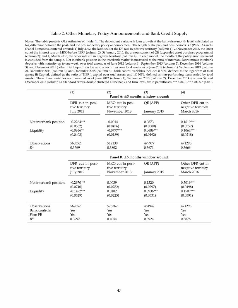
Our analysis suggests that NIRP works differently from conventional monetary policy. The stan-

dard bank lending channel postulates that monetary easing has a greater impact on credit supply for

banks with lower liquid-to-total assets ratios (Kashyap and Stein, 1995, 2000; Jiménez et al., 2012).9

This is indeed what we find even for the previous rate cuts just above the ZLB, both for the 2012

deposit facility (DF) rate cut and the 2013 main refinancing operation (MRO) rate cut. By contrast,

an interest rate cut into negative territory works differently, with stronger effects for banks with larger

liquid-to-total assets ratios.

We document that the introduction of NIRP steered market expectations by removing the ZLB,

inducing a downward shift and a simultaneous flattening of the yield curve (see also: Draghi, 2016;

Cœuré, 2017; Grisse et al., 2017), which previous rate cuts above the ZLB had been unable to achieve.10

9Drechsler et al. (2017) focus on the effect of market power in the deposits market as opposed to that of bank balancesheet liquidity.

10Before the announcement of NIRP, with the overnight interest rate at the perceived lower bound, the distributionof future possible rates is truncated: expected future short-term interest rates can only increase. The announcement ofnegative rates removes the perception of the lower bound at zero and hence change the distribution of expected futureshort-term interest. Christensen (2019) shows that the yield curve flattened after the announcement of NIRP in all countries

11

Moreover, we further document that the decline in the yields of safer, liquid assets of all maturities

widened the wedge vis-a-vis yields on riskier assets, incentivizing banks to rebalance their portfolios.

We find similar results for the last rate cut (with available data) in March 2016.

Finally, we show that also the ECB’s January 2015 announcement of QE policies is associated

with a strong flattening of the yield curve and bank portfolio rebalancing effects. Despite the fact

that both QE and NIRP announcements flattened the yield curve, the two policies differ as NIRP was

additionally associated with a drop in very short-term rates, which penalizes holdings of very short-

term interbank claims even more than QE. As a result, we find that the coefficient estimate on bank

liquidity is similar around QE and NIRP announcements, but the coefficient on the net interbank

position is smaller and insignificant for QE compared to its NIRP counterpart.

Contribution to the literature. Our main contribution to the literature is to show expansionary ef-

fects of NIRP, yet different from rate cuts just above the ZLB. By shifting down and flattening the yield

curve, NIRP activated a portfolio rebalancing channel. On the other hand, we do not find evidence

of a retail deposits channel associated with NIRP. Our evidence that negative rates are expansionary

through banks lends support to the view that monetary policy does not necessarily become ineffec-

tive at the ZLB (Rognlie, 2016; Swanson, 2018; Debortoli et al., 2019). We also provide estimates of

the elasticity of credit with respect to bank balance sheet variables that capture different transmission

channels of NIRP to lending. Thus, our results inform macro models on the transmission of NIRP to

the real economy through the bank lending channel, in the spirit of Nakamura and Steinsson (2018),

and support models that emphasize the portfolio rebalancing effects of NIRP over the retail deposits

channel, with an expansionary effect on lending and the real economy.

Our analysis adds to several recent studies of the impact of NIRP on bank lending. Eggertsson

et al. (2019) examine the effects of NIRP through the retail deposits channel. Using bank-level data

and variation in the share of deposit funding across Swedish banks, the authors document a weak-

ening pass-through from the policy rate to loan rates during the NIRP period. By contrast, we use

loan-level data and document a strong pass-through from negative policy rates to loan rates while

controlling for shifts in unobserved time-varying firm-level characteristics. Heider et al. (2019) ex-

amine the effects of negative rates from June 2014 on syndicated loans in the euro area. Based on a

difference-in-differences estimation that exploits variation in reliance on retail deposits across banks

as a measure of exposure to NIRP, the authors show that banks with more retail deposits (hence

which adopted negative rates (not only Euro area but also Denmark, Sweden, Switzerland and Japan).

12

more constrained in passing negative rates to depositors) reduce syndicated loan growth and take

more risk than other banks. In our analysis, based on more granular and comprehensive data from a

country with a large presence of bank-dependent small and medium-sized firms, the retail deposits

channel is inactive. In addition, we show that NIRP has expansionary effects on credit supply and,

in turn on the real economy, through a portfolio rebalancing channel.11

Our paper further contributes to the broader literature on unconventional monetary policy, which

focuses on more common policies such as large-scale asset purchases, large liquidity injections and

forward guidance (see, among others, Bhattarai and Neely (2016); Chakraborty et al. (2019); and

Rodnyansky and Darmouni (2017) for U.S. policies; and Acharya et al. (2016); Acharya et al. (2019)

and Peydró et al. (2017) for European policies).12 Finally, our paper adds to the literature on the

risk-taking channel of monetary policy (see Adrian and Shin, 2010; Jiménez et al., 2014; Dell’Ariccia

et al., 2017, among others). Our main contribution to these two strands of literature is to analyze the

portfolio rebalancing channel of negative interest rates, its effects on bank credit and the real economy

and show why NIRP differs from previous rate cuts above the ZLB.

The remainder of the paper is organized as follows. Section 1 discusses the negative interest rate

policy of the ECB. Section 2 describes the data, hypotheses, and empirical approach. Sections 3 and 4

document the effects of NIRP on credit supply and firm-level outcomes. Section 5 concludes.

11Basten and Mariathasan (2018) and Demiralp et al. (2019) use bank-level data and take excess reserves at the centralbank as a measure of sensitivity to negative policy rates. In Italy, excess reserves are close to zero. Demiralp et al. (2019)show that European banks with more excess liquidity expand lending, consistent with our results about a portfolio re-balancing channel. They find no evidence of a retail deposits channel. Basten and Mariathasan (2018) look at the case ofSwitzerland to examine a policy decision aimed at mitigating currency appreciation in a safe-haven country facing strongcapital inflows. They find that bank profitability is unaffected by NIRP, as banks offset lower-interest margins with higherfees, but banks take more risk. Arseneau (2017) uses supervisory data from the U.S. bank stress tests, in which U.S. banksare asked about the balance sheet impact of hypothetical NIRP, and finds that U.S. banks vary significantly in their exposureto negative rates and the effect of NIRP on bank margins would depend on their liquidity provision. Altavilla et al. (2019)show that negative rates in Europe have an expansionary effect through a corporate channel, as firms more exposed tothe policy (holding cash at banks that pass through negative rates to depositors) rebalance their portfolio from cash andshort-term assets to investment. None of these studies use micro data at loan level, so they cannot control for unobservedtime-varying firm-level characteristics such as credit demand and risk. Finally, Arce et al. (2018) compare the lendingbehavior of Spanish banks that reported to the ECB’s Bank Lending Survey their views on the incidence of NIRP on netinterest income in April 2016 (that is, two years after the introduction of NIRP). Their analysis shows that the banks whichreported profitability had been negatively impacted by this policy took less risk in their loan portfolio and that credit sup-ply did not change differentially across banks. Compared to the approach of this paper, our measures of bank exposureto NIRP are computed prior to the policy (not ex-post), they are grounded in a specific transmission channel of monetarypolicy (namely, the portfolio rebalancing channel), and they rely on supervisory data as opposed to being self-reported.

12For theoretical contributions on unconventional monetary policy, see Gertler and Karadi (2011), Curdia and Woodford(2011) and McKay et al. (2016), among others.

13

2 Institutional Background

In this section we discuss the institutional context in which the ECB introduced NIRP and the details

of its implementation. In doing so, we lay out the key elements of our empirical strategy.

Italy is a part of a monetary union, and hence unlike most countries around the world (such as US,

UK, Japan, etc.), monetary policy is not decided by its own central bank, but by the European Central

Bank for the entire euro area. Before NIRP, monetary conditions had been tighter in Italy than in

several other European countries and the U.S.13 In Italy, GDP growth was negative in both 2012 and

2013. At that time, the ECB had not yet introduced QE and its balance sheet was shrinking (partly

due to early LTRO repayments). By contrast, the U.S. Federal Reserve and the Bank of England

already had introduced large scale asset purchase programs (LSAPs) and their balance sheets were

expanding. Against the backdrop of negative GDP growth and low and declining inflation in 2013,14

the ECB decided to cut rates into negative territory in mid-2014. These developments suggest that

ECB’s monetary policy in June 2014 did not directly address the macroeconomic context in Italy, but

rather the slowdown in economic recovery in the euro area as a whole, with the goal of maintaining

price stability in the area.

The ECB is not the only central bank to implement NIRP. Since 2012, other major central banks

around the world have adopted negative monetary policy rates in an effort to either further ease

monetary conditions and to support economic activity (e.g., Japan) or to limit capital inflows and

related exchange rate appreciation (e.g., Switzerland and Denmark). In August 2019, monetary rates

were negative in countries accounting for 25% of world GDP and the amount of debt globally trad-

ing at negative yields reached USD 17 trillion.15 On June 11, 2014, the ECB reduced the deposit

facility (DF) rate—the rate it pays on overnight deposits with the central bank in excess of reserve

requirements (“excess reserves”)—to−0.10%.16 The rationale behind this rate cut was to further ease

monetary conditions by pushing down yields and borrowing costs and to encourage banks to invest

13Not only compared to other euro area countries, but also to Switzerland and Sweden, both of which introduced nega-tive policy rates.

14In fact, the inflation rate was below 1% at the end of 2013 and further declined in 2014, turning to deflation by the endof the year.

15Source: “Market Swing on Trade and Monetary Policy”, September 2019, BIS Quarterly Review, Bank of InternationalSettlements.

16Euro area banks are required to hold a certain amount of funds as reserves in their current accounts at their nationalcentral bank (minimum reserve requirement), which are remunerated at the main refinancing operation rate. Further, theycan hold reserves in excess to the minimum reserve requirement either in the Eurosystem deposit facility or as reserveholdings in their current accounts. Differently from the past, ever since the ECB introduced a negative rate on the depositfacility, it treats the current account balances (in excess of the minimum reserve requirement) and the deposit facility in thesame way. Both yield negative rates.

14

in alternative assets, boosting their prices. In the words of Hutchinson and Smets (2017, p. c3), “the

rationale of this measure was that by extending the scope of conventional monetary policy beyond the ZLB, the

entire distribution of short-term rates was shifted downwards and additional stimulus could be provided to the

economy.” The ECB further cut its DF rate to −0.20% on September 10, 2014, to −0.30% on December

9, 2015, to −0.40% on March 16, 2016 and, finally, to −0.50% on September 18, 2019.

Short-term interbank rates dropped and entered negative territory soon after the June 2014 cut

of the DF rate. The Euro OverNight Index Average (EONIA), a measure of the cost of funds on the

Eurozone overnight interbank market, turned negative for the first time in August 2014. Soon after,

the one-week Euro Interbank Offered Rate (EURIBOR) became negative as well and stayed below

zero for the entire period of analysis (see Figure 1). Around the NIRP announcement, the declines in

the interbank rates at one-month and three-month maturities were smaller and both rates remained

positive throughout the period.

Importantly, the announcement of NIRP also impacted the middle and long end of the yield curve.

In fact, the entire yield curve shifted downward and flattened (see Figure 2). The fall in the yield of

safer assets across all maturities widened the wedge between the yields of safer, more liquid assets

and those of riskier, more illiquid assets. (We discuss these developments and the role they play in

our results in further detail in Section 2.2.)

In May 2014, the growth rate of bank credit to businesses in Italy was negative, at -4.7% on a yearly

basis, in an environment of depressed aggregate demand. As shown in Figure 3, immediately after

the introduction of NIRP, credit growth picked up, reaching -3.1% at the end of June 2014. While still

negative, it continued to rise, reaching -2.3% in December 2014. Besides reflecting demand dynamics,

for which we carefully control in the analysis, these developments may have benefitted from other

ECB monetary policies implemented around the same time as NIRP. Notably, on June 5, 2014 the

ECB announced its TLTRO program and deployed it starting in September 2014. The program aimed

at boosting bank credit by offering long-term funding to Eurozone banks on attractive terms. If the

TLTRO had an expansionary effect on the economy before its implementation and if banks’ take-up

of TLTRO funds was correlated with their March 2014 net interbank and liquidity positions, we may

incorrectly attribute our estimated effects to the NIRP instead of this policy. To address this potential

concern, we control for the TLTRO with a bank-level measure of ex-ante capacity to borrow under the

TLTRO, derived from supervisory data. Furthermore, Benetton and Fantino (2018) show that while

TLTRO reduced the costs of credit for Italian firms, it only did so after the implementation of the

second round of the program, that is, only in the second and third quarter of 2015, and hence outside our

15

baseline time window. (We discuss the TLTRO in more detail and show our main results are robust

to controlling for this policy in Section 3.1.)

Furthermore, a few months later, on January 22, 2015, the ECB announced the expansion of its

limited Asset Purchase Program (APP). This policy action, implemented starting March 9, 2015, was

widely seen as the start of the ECB’s QE, with the objective of providing additional monetary pol-

icy stimulus and further easing borrowing conditions of households and firms. Specifically, the ECB

expanded its existing, quantitatively limited asset-purchase programs of covered bonds and asset-

backed securities to include public-sector bonds for a total of 60 billion euros worth of monthly pur-

chases.17 Both the announcement and the implementation of this program are largely outside the

time window of our baseline results, so we can rule out the APP affecting our estimates. That said,

we also analyze the effects of this LSAP QE policy (in addition to previous conventional and uncon-

ventional monetary policies) and compare them with NIRP, in order to understand whether—and

why—NIRP is special.

3 Data and Empirical Hypotheses

In this section we explain the different datasets, empirical hypotheses and identification. For empiri-

cal identification, we exploit several matched administrative datasets, together with the introduction

of NIRP and other policy rate cuts. For the associated mechanisms, we exploit differences in ex-ante

bank balance sheet characteristics that are consistent with different channels of transmission (portfo-

lio rebalancing vs. retail deposits), credit supply via volume and loan rates in a within-firm setting,

and the change in the yield curve. We also discuss our data and empirical strategy for the analysis of

the associated real effects.

3.1 The Credit Register and Other Data

We employ a double-matched administrative bank-firm monthly panel dataset covering the lend-

ing activities of Italian banks between 2012 and 2016. The dataset draws on three sources: (i) the

loan-level credit register of the Bank of Italy, which reports outstanding loan exposures (with min-

imum size of 30,000 euros) of all banks operating in Italy vis-a-vis Italian non-financial firms; (ii)

17The initial asset-purchase programs of covered bonds (CBPP3) and asset-backed securities (ABSPP) were announcedin September 2014 and implemented, respectively, in October and November 2014. These initial purchases were so limitedquantitatively that only the announcement of January 2015 is considered to be the start of the ECB QE programme, alsocalled LSAP (see, for instance, Altavilla et al. (2015) or Gambetti and Musso (2017)). That said, in Section 3.1 we show thatour results are robust even if we consider a very narrow window of one month around the NIRP announcement.

16

supervisory data on bank balance sheets; and (iii) data on firm financials from the proprietary CADS

database, owned by Cerved Group, a member of the European Committee of Central Balance-Sheet

Data Offices that collects official balance sheet data reported by firms to the Chambers of Commerce,

as required by Italian law. All data are monthly, with the exception of firm financials which are yearly

and selected bank balance sheet variables which are quarterly (such as capital and net interbank po-

sition) or semiannual (income from fees).

Given the relatively small loan size threshold for inclusion of loans in the credit register, cover-

age of the credit register is almost universal, comprising all firms with banking relationships. We

drop foreign bank branches and subsidiaries (as their liquidity depends on foreign headquarters)

and cooperative or mutual banks (as they are subject to different regulations). Our final regression

sample contains more than 167,000 firms with multiple banking relationships, borrowing from 95

banks. Loan exposures refer to credit lines, overdraft facilities and term loans.

Data on loan interest rates come from a special section of the credit register (Taxia) and are re-

ported by a representative sample of the largest banking groups and individual banks (covering

more than 80% of total bank lending in Italy).18

For a robustness test, we also use data from the securities register at the Bank of Italy, with in-

formation on the holdings of each security held by each bank in each month, coupled with data on

securities yields and prices from Thomson Reuters Eikon, on the basis of which we construct a bank-

level measure of windfall gains (defined as profits or losses due to the revaluation of the securities in

the portfolios).

Italian banks play a key role in financing the real economy, as most borrowers are small or

medium-size enterprises with limited access to alternative sources of external financing. Commercial

banks have a traditional business model focused on loan intermediation and banking services. Retail

deposits (collected almost entirely from domestic residents) account for 69% of total funding, whole-

sale funding for 24%, and Eurosystem financing for the remaining 7%. On the asset side, loans to the

private sector account for 39% of total assets (with loans to non-financial firms at 60% of the average

bank’s loan book).

18For each credit relationship with commitments above 75,000 euros, banks report two numbers each quarter: first, theamount paid as interest and second, the amount of the loan outstanding times the days the amount was outstanding. If theoutstanding amount is 100,000 euros for 45 days and 150,000 for the remaining 45 days of the quarter, the reported numberis 100,000×45+150,000×45. By dividing the interest payments by the second number we obtain the interest rate paid onthe loan, which we annualize (see Sette and Gobbi, 2015).

17

3.2 Identification Strategy

3.2.1 Portfolio Rebalancing vs. Retail Deposits Channel

In the words of the ECB President Mario Draghi: “negative [policy] rates were introduced for one specific

reason: when interest rates reached the zero lower bound, the expectations for the future rates in the long

term are only that the rates can go up. So with negative rates we were successful in taking these expectations

down” (Draghi, 2016). NIRP puts downward pressure on the yields of bank liquid assets and shifts

banks’ risk-reward calculus for asset allocation, with loans becoming more attractive (Bernanke, 2016;

Rostagno et al., 2016). However, when interest rates become negative, profit margins can also shrink if

banks do not pass through short-term funding rates to retail deposits (Heider et al., 2019; Eggertsson

et al., 2019). Therefore, both a portfolio rebalancing channel and a retail deposits channel may operate

simultaneously.

We conduct a cross-sectional analysis of bank balance sheets to show that Italian banks with

more retail deposits before the introduction of negative rates did not experience a relative decline

in profitability in the 6 months after NIRP (Table A1). In addition, we find evidence suggesting that

banks were able to compensate for the compression of intermediation margins from incomplete pass-

through of negative rates to retail deposit rates with higher fees on banking services. Table A2 shows

that banks with greater retail deposits obtain higher income from fees for banking services related to

the holdings of deposits in the months following the introduction of NIRP. These findings suggest

that the retail deposits channel may be inactive in the Italian context; we directly test this hypothesis

in Section 3.

3.2.2 Portfolio Rebalancing Channel and Bank Exposure Variables

To identify the portfolio rebalancing channel, we focus on two measures of bank exposure to NIRP:

first, the net interbank position and, second, a broader measure of balance sheet liquidity. Both

measures are computed prior to the enactment of the policy.

The European interbank market is very large and is mainly concentrated in short-term maturities

(Upper, 2006). Interest rates in this market were immediately affected by NIRP. The one-week Euro

Interbank Offered Rate (EURIBOR) experienced the largest drop compared with interbank rates at

longer maturities and soon even became negative. Given that banks generally act as both lenders

and borrowers in the interbank market (Angelini et al., 2011; Acharya and Merrouche, 2012), we

measure bank-level exposure to NIRP with the net interbank position, computed as the difference

18

between interbank loans and interbank deposits with maturity up to one week, divided by total

assets. This measure includes all loans and deposits with banks, both domestic and foreign, as well

as repos. Interbank lending at maturities up to one week represents about 70% of total activities in

the interbank market.

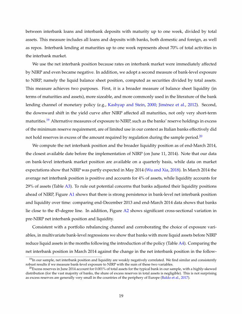
We use the net interbank position because rates on interbank market were immediately affected

by NIRP and even became negative. In addition, we adopt a second measure of bank-level exposure

to NIRP, namely the liquid balance sheet position, computed as securities divided by total assets.

This measure achieves two purposes. First, it is a broader measure of balance sheet liquidity (in

terms of maturities and assets), more sizeable, and more commonly used in the literature of the bank

lending channel of monetary policy (e.g., Kashyap and Stein, 2000; Jiménez et al., 2012). Second,

the downward shift in the yield curve after NIRP affected all maturities, not only very short-term

maturities.19 Alternative measures of exposure to NIRP, such as the banks’ reserve holdings in excess

of the minimum reserve requirement, are of limited use in our context as Italian banks effectively did

not hold reserves in excess of the amount required by regulation during the sample period.20

We compute the net interbank position and the broader liquidity position as of end-March 2014,

the closest available date before the implementation of NIRP (on June 11, 2014). Note that our data

on bank-level interbank market position are available on a quarterly basis, while data on market

expectations show that NIRP was partly expected in May 2014 (Wu and Xia, 2018). In March 2014 the

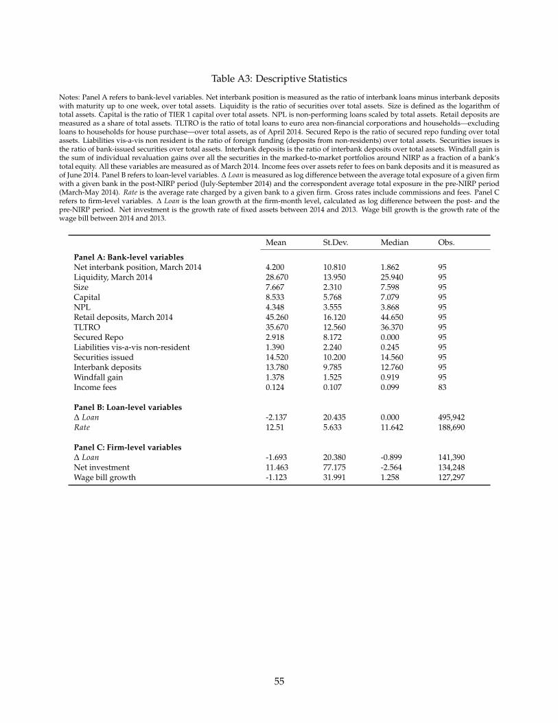
average net interbank position is positive and accounts for 4% of assets, while liquidity accounts for

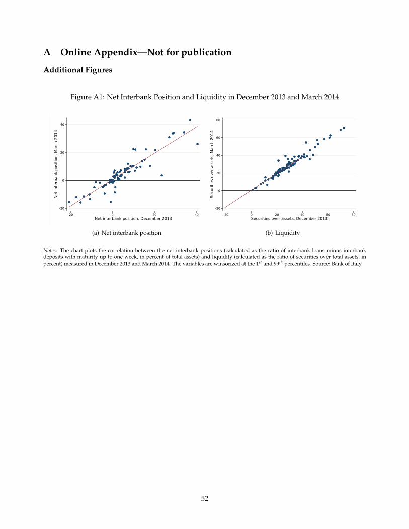
29% of assets (Table A3). To rule out potential concerns that banks adjusted their liquidity positions

ahead of NIRP, Figure A1 shows that there is strong persistence in bank-level net interbank position

and liquidity over time: comparing end-December 2013 and end-March 2014 data shows that banks

lie close to the 45-degree line. In addition, Figure A2 shows significant cross-sectional variation in

pre-NIRP net interbank position and liquidity.

Consistent with a portfolio rebalancing channel and corroborating the choice of exposure vari-

ables, in multivariate bank-level regressions we show that banks with more liquid assets before NIRP

reduce liquid assets in the months following the introduction of the policy (Table A4). Comparing the

net interbank position in March 2014 against the change in the net interbank position in the follow-

19In our sample, net interbank position and liquidity are weakly negatively correlated. We find similar and consistentlyrobust results if we measure bank-level exposure to NIRP with the sum of these two variables.

20Excess reserves in June 2014 account for 0.001% of total assets for the typical bank in our sample, with a highly-skeweddistribution (for the vast majority of banks, the share of excess reserves in total assets is negligible). This is not surprisingas excess reserves are generally very small in the countries of the periphery of Europe (Baldo et al., 2017).

19

ing 6 months (between March and September 2014) shows that banks with greater ex-ante exposure

are more likely to reduce their net position in the short-term interbank market (column 1) and this

reduction is achieved by curtailing interbank lending (column 2) rather than increasing interbank

borrowing (column 3). Similarly, we find that banks with more liquidity in March 2014 reduce the

amount of liquid assets held on their balance sheets between March and September 2014 (column 4).

3.2.3 NIRP, the Yield Curve, and Portfolio Rebalancing Channel

What is different about the portfolio rebalancing channel during NIRP, compared to previous rate

cuts just above the ZLB? According to Benoît Cœuré, Member of the Executive Board of the ECB,

“with short-term policy rates approaching levels closer to zero during the early phases of the most recent easing

cycle, this channel had become less effective” (Cœuré, 2017). He goes on to argue that when the ECB

changes the key policy rates during normal times, the central bank is able to directly impact the short

end of the yield curve, which is the basis of the expectations component. To the extent that mar-

ket participants see a change in policy rates as the beginning of an incremental series of changes,

longer-term rates adjust accordingly. However, in the years before NIRP, market participants be-

lieved negative rates were unrealistic and were therefore not pricing the degree of accommodation

they normally would have expected. In other words, when nominal rates approach the ZLB, the

transmission of short-term policy rate cuts to long-term rates becomes weaker (Ruge-Murcia, 2006).

In Cœuré (2017) words, the “decision in June 2014 to introduce negative deposit facility rates restored

our ability to steer market expectations, [. . . ] by signaling to the market that policy rates could go below zero, we

ultimately succeeded in shifting downwards the entire distribution of future expected short-term rates, thereby

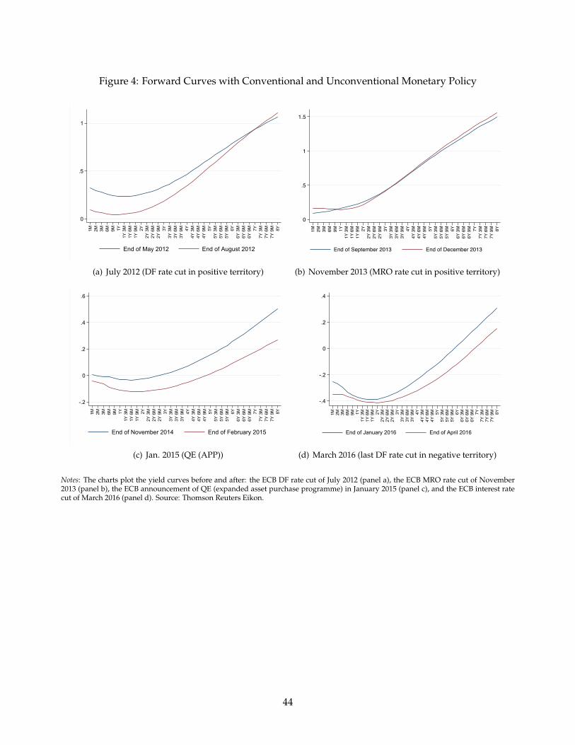
providing important additional accommodation.”21 In Figure 2 we document that this was indeed the case.

We observe both a downward shift and a flattening of the yield curve only after NIRP and not after

the previous rate cuts (above the ZLB) in July 2012 and November 2013 (Figure 4, panels a and b).

Rostagno et al. (2016) conclude that NIRP was able to “rehabilitate monetary policy in the low rate world”.

Through their impact on the yield curve, negative nominal interest rates reinstated the transmission

of monetary policy and facilitated a reallocation of bank assets, with potential benefits for lending

21Lemke and Vladu (2017) show theoretically that this was indeed the case. By pushing down the effective lower bound,negative policy rates enabled current and future rates to be negative. In their model, the introduction of NIRP makes theforward curve flatter than it would be if short rates are expected to be constrained by a zero lower bound. An event studyof yield reactions to negative interest rate announcements shows that long rates tend to drop in response to downwardrevisions in the market’s believed location of the lower bound (Grisse et al., 2017). Eisenschmidt and Smets (2017) make asimilar point by showing the empirical discontinuity in the shape of the forward curve around the introduction of NIRP inJune 2014.

20

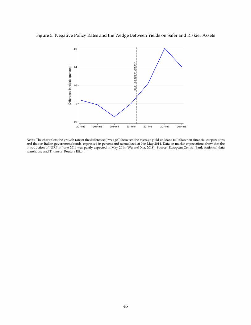
and the real economy. In Figure 5 we show that NIRP was indeed able to generate incentives for

portfolio reallocation. The fall in the yield of safer assets of all maturities opened a wedge between

the yields on safer, more liquid assets (proxied by Italian government bonds) and yields on riskier

assets (loans to Italian non-financial firms). The wedge emerged in May 2014, consistent with the

announcement of NIRP being partly expected the month before the announcement (Wu and Xia,

2018). This development is similar with the increase in the safety premium after QE programs of the

Federal Reserve, as documented by Krishnamurthy and Vissing-Jorgensen (2011).

In Figure 4 (panel c) we show that a similar flattening of the yield curve took place in January

2015 when the ECB announced its first LSAP QE (via the expanded APP), a feature documented

by Eser et al. (2019). In Section 3.4 we conduct a comprehensive comparison between NIRP and

other monetary events, including two preceding interest rate cuts near but above the ZLB, and the

QE (APP) announcement (see Figure 4). Finally, one may argue that that a flat yield curve puts

downward pressure on net interest income in the long run, as the margin between lending rates and

borrowing costs compresses (Adrian and Shin, 2010). Despite this possibility, in 2014 and 2015 the

net income of large euro area banking groups actually increased. Even net interest income made a

positive contribution despite a small decline in interest margins. This reflects an increase in credit

volumes after NIRP (ECB, 2016).

3.3 Empirical Specifications

Impact on loan volumes and rates. To identify the effect of negative policy rates on credit supply,

we compare loan volumes of banks with different levels of exposure to NIRP before and after the

ECB’s enactment of this policy in June 2014. Moreover, we also use how banks differently exposed to

NIRP change loan rates to the same firm at the same time, i.e. exploiting whether credit volumes vs.

rates (depending on bank exposure to NIRP) change in the same way (both increase, consistent with

demand), or they change in different way (consistent with supply). We first use the classic Khwaja

and Mian (2008) approach and collapse the monthly credit register data into a single pre- and post-

NIRP period, with windows of ±3 and ±6 months around June 2014.22 We also analyze other rate

cuts (before and after the June 2014 introduction of NIRP), as well as QE. We compute loan growth at

the bank-firm level (∆Loanib) as the log difference in total loans granted by bank b to firm i between

22Given that the policy was announced in mid-June 2014, we drop all the observations of this month from the sample.We keep the period of analysis relatively short to minimize the impact of other potentially confounding ECB policies. Weperform several robustness tests related to the timing of NIRP introduction and the length of windows around it (and wealso analyze a very short-term window of ±1 month); see Table A8 and related discussion in Section 3.2.

21

the post- and the pre-NIRP periods, and estimate the following equation:

∆Loanib = α Net interbank positionb + β Liquidityb + γ′Xb + φi + εib, (1)

where the measures of NIRP exposure are the net interbank position and liquidity (both defined in

Section 2.2.2). Given that our measures of bank exposure to negative rates could be correlated with

other bank characteristics (Table A5), to isolate the effect of NIRP on bank credit supply through

the portfolio rebalancing channel, we include the vector Xb of bank controls, all measured at end-

March 2014: bank size (the logarithm of total assets), regulatory capital (Tier 1 capital divided by total

assets), and NPLs (impaired loans divided by total assets)—note also that since the model analyzes

differences in credit, not levels, we implicitly control for bank fixed effects.23 Furthermore, note that

there is no systematic relationship between a comprehensive set of firm observables (including size,

riskiness measured as distance from default, leverage, and profitability) and bank NIRP exposure,

measured either by the net interbank position or liquidity (see Table A6).24

Shifts in credit demand and other unobserved firm-specific shocks are captured by firm fixed

effects (φi), so the coefficients of interest α and β are identified by comparing the change in credit to

the same firm in the same period by banks with different NIRP exposure. Regression estimates are

obtained with the Ordinary Least Squares (OLS) estimator and standard errors are double-clustered

at the bank and firm level. Double-clustering allows for residual correlation within banks, since our

treatment variable varies at the bank level, as well as within firms, given that credit growth to the

same firm may be correlated across banks (for firms with many banking relationships and not fully

absorbed by firm fixed effects). As shown in the next Section, we subject the baseline specification to

many robustness tests.

As explained above, we adopt a similar approach to test for the impact of NIRP on loan rates,

where the dependent variable is the change in loan rates applied to loans granted by bank b to firm

i between the post- and the pre-NIRP periods, focusing on a ±6 month window around June 2014.

Descriptive statistics for regression variables are reported in Table A3. If the portfolio rebalancing

23While net interbank position is negatively correlated with size, liquidity is negatively correlated with capital and NPLs(Table A5). Moreover, we analyze the same model in other periods to check whether results are driven by NIRP vs. othermonetary policies, or by bank unobservables.

24We test for the balancing of covariates computing the normalized difference between each quartile average and theaverage in the other three quartiles. To avoid that results depend on sample size, we follow Imbens and Wooldridge (2009)and analyze the normalized differences—which are the differences in averages over the square root of the sum of thevariances. Imbens and Wooldridge (2009) propose as a rule of thumb a 0.25 threshold in absolute terms, i.e. two variableshave “similar” means when the normalized difference does not exceed one quarter. Results confirm that firm observablesare well balanced across the distribution of bank exposure to NIRP.

22

by banks due to negative rates is at work, the supply of credit volume by more affected banks will

increase, while loan rates will decrease, consistent with a bank (supply) driven mechanism.

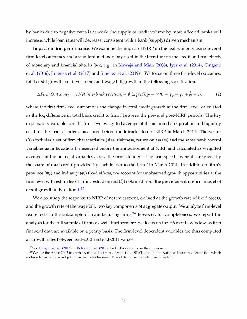
Impact on firm performance. We examine the impact of NIRP on the real economy using several

firm-level outcomes and a standard methodology used in the literature on the credit and real effects

of monetary and financial shocks (see, e.g., in Khwaja and Mian (2008), Iyer et al. (2014), Cingano

et al. (2016), Jiménez et al. (2017) and Jiménez et al. (2019)). We focus on three firm-level outcomes:

total credit growth, net investment, and wage bill growth in the following specification:

∆Firm Outcomei = α Net interbank positioni + β Liquidityi + γ′Xi + ψp + φs + δ̂i + εi, (2)

where the first firm-level outcome is the change in total credit growth at the firm level, calculated

as the log difference in total bank credit to firm i between the pre- and post-NIRP periods. The key

explanatory variables are the firm-level weighted average of the net interbank position and liquidity

of all of the firm’s lenders, measured before the introduction of NIRP in March 2014. The vector

(Xb) includes a set of firm characteristics (size, riskiness, return on assets) and the same bank control

variables as in Equation 1, measured before the announcement of NIRP and calculated as weighted

averages of the financial variables across the firm’s lenders. The firm-specific weights are given by

the share of total credit provided by each lender to the firm i in March 2014. In addition to firm’s

province (ψp) and industry (φs) fixed effects, we account for unobserved growth opportunities at the

firm level with estimates of firm credit demand (δ̂i) obtained from the previous within-firm model of

credit growth in Equation 1.25

We also study the response to NIRP of net investment, defined as the growth rate of fixed assets,

and the growth rate of the wage bill, two key components of aggregate output. We analyze firm-level

real effects in the subsample of manufacturing firms;26 however, for completeness, we report the

analysis for the full sample of firms as well. Furthermore, we focus on the±6 month window, as firm

financial data are available on a yearly basis. The firm-level dependent variables are thus computed

as growth rates between end-2013 and end-2014 values.

25See Cingano et al. (2016) or Bofondi et al. (2018) for further details on this approach.26We use the Ateco 2002 from the National Institute of Statistics (ISTAT), the Italian National Institute of Statistics, which

include firms with two-digit industry codes between 15 and 37 in the manufacturing sector.

23

4 Credit Supply

4.1 Main Results

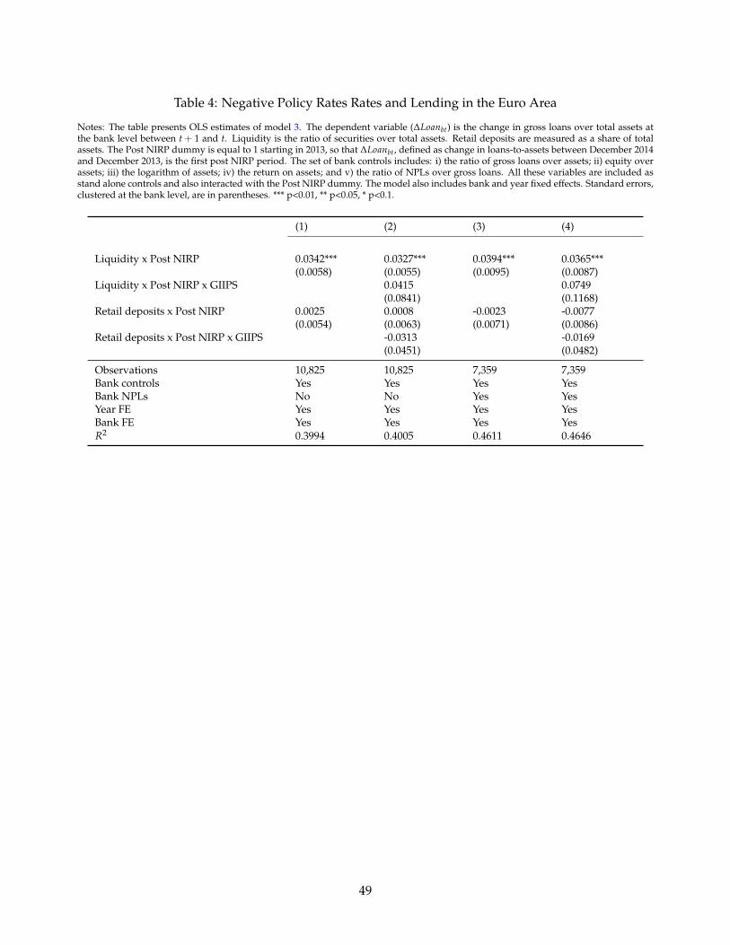
Baseline Results. Table 1 shows the results from our baseline lending regressions for two time win-

dows: ±3 and ±6 months around June 2014. For each case, we start by including separately the net

interbank position and liquidity (respectively, columns 1 and 2) and then we include both variables

at the same time (column 3).

The coefficient on the net interbank position is positive, statistically significant and stable across

model specifications, and indicates that banks with greater net interbank position before NIRP in-

crease credit supply after the introduction of NIRP more than other banks. The estimated effect of

the policy is economically significant. One standard deviation increase in net interbank position is

associated with a relative increase of 1.4 percentage points in credit supply after 3 months by more

exposed banks (based on the coefficient in column 3 of Table 1). This effect is 1.9 percentage points

after 6 months.

The estimated coefficient on bank liquidity is also positive, suggesting that banks with more liq-

uid balance sheets react to NIRP by expanding credit supply more than less liquid banks. The mag-

nitude of the effect of liquidity is comparable to that of the net interbank position, as a change in

one standard deviation of liquidity is associated with an increase in credit supply by 0.8 percentage

points after 3 months and 1 percentage point after 6 months. Given that the average growth rate of

credit was -2.1% over the sample period, these effects are economically sizable.

Overall, the results in Table 1 provide evidence for a portfolio rebalancing channel of monetary

policy transmission from liquidity to credit supply in an environment of negative interest rates. They

confirm our conjecture that NIRP affects banks through liquidity management. Interestingly, they are

also the opposite of how the bank lending channel works in normal times, when banks with more

liquid balance sheets react less to monetary policy shocks (Kashyap and Stein, 2000).

The Retail Deposits Channel. As discussed in Section 2.2.1, negative policy rates can also affect

banks’ credit supply through a compression in deposit margins. Given that banks may generally be

unwilling to pass negative interest rates to retail depositors, there is a potential cost associated with

higher retail deposits when monetary policy rates become negative (Heider et al., 2019; Eggertsson

et al., 2019). To test this channel, in column 4 of Table 1 we control for banks’ reliance on retail deposits

(as a share of total assets). The results show no evidence of a retail deposits channel across the time

windows considered. Moreover, the coefficient estimates on our key NIRP-exposure variables remain

24

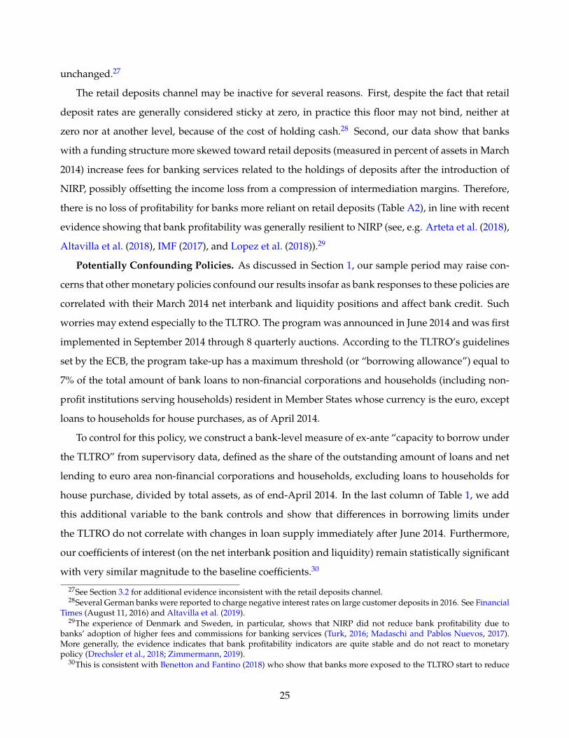
unchanged.27

The retail deposits channel may be inactive for several reasons. First, despite the fact that retail

deposit rates are generally considered sticky at zero, in practice this floor may not bind, neither at

zero nor at another level, because of the cost of holding cash.28 Second, our data show that banks

with a funding structure more skewed toward retail deposits (measured in percent of assets in March

2014) increase fees for banking services related to the holdings of deposits after the introduction of

NIRP, possibly offsetting the income loss from a compression of intermediation margins. Therefore,

there is no loss of profitability for banks more reliant on retail deposits (Table A2), in line with recent

evidence showing that bank profitability was generally resilient to NIRP (see, e.g. Arteta et al. (2018),

Altavilla et al. (2018), IMF (2017), and Lopez et al. (2018)).29

Potentially Confounding Policies. As discussed in Section 1, our sample period may raise con-

cerns that other monetary policies confound our results insofar as bank responses to these policies are

correlated with their March 2014 net interbank and liquidity positions and affect bank credit. Such

worries may extend especially to the TLTRO. The program was announced in June 2014 and was first

implemented in September 2014 through 8 quarterly auctions. According to the TLTRO’s guidelines

set by the ECB, the program take-up has a maximum threshold (or “borrowing allowance”) equal to

7% of the total amount of bank loans to non-financial corporations and households (including non-

profit institutions serving households) resident in Member States whose currency is the euro, except

loans to households for house purchases, as of April 2014.

To control for this policy, we construct a bank-level measure of ex-ante “capacity to borrow under

the TLTRO” from supervisory data, defined as the share of the outstanding amount of loans and net

lending to euro area non-financial corporations and households, excluding loans to households for

house purchase, divided by total assets, as of end-April 2014. In the last column of Table 1, we add

this additional variable to the bank controls and show that differences in borrowing limits under

the TLTRO do not correlate with changes in loan supply immediately after June 2014. Furthermore,

our coefficients of interest (on the net interbank position and liquidity) remain statistically significant

with very similar magnitude to the baseline coefficients.30

27See Section 3.2 for additional evidence inconsistent with the retail deposits channel.28Several German banks were reported to charge negative interest rates on large customer deposits in 2016. See Financial

Times (August 11, 2016) and Altavilla et al. (2019).29The experience of Denmark and Sweden, in particular, shows that NIRP did not reduce bank profitability due to

banks’ adoption of higher fees and commissions for banking services (Turk, 2016; Madaschi and Pablos Nuevos, 2017).More generally, the evidence indicates that bank profitability indicators are quite stable and do not react to monetarypolicy (Drechsler et al., 2018; Zimmermann, 2019).

30This is consistent with Benetton and Fantino (2018) who show that banks more exposed to the TLTRO start to reduce

25

Another relevant ECB policy is the first LSAP QE (APP). However, the QE announcement took

place on January 22, 2015, that is, more than 3 months after the end of the time window of our

baseline results. As a result, QE is unlikely to affect our estimates. In Section 3.4 we focus on QE to

test whether it also affected credit supply through a portfolio rebalancing channel.

To address any residual concerns that our results may be driven by other ECB policies in the time

window of our main regressions—such as the second reduction of DF rates, the implementation of

the TLTRO or the very limited purchases of asset-backed securities and covered bonds announced

in September 2014 (all discussed in Section 1), we shrink the window of analysis. Specifically, we

estimate specifications in which we compute loan growth as the log difference in total loans granted

between July 2014 (the 1-month post-NIRP window) and April 2014 (the 1-month pre-NIRP window).

Given that the introduction of NIRP was already expected by market participants in May 2014 (Wu

and Xia, 2018), we drop observations from both May and June from the sample. As seen in Table

A7 (columns 1-3), evidence for the portfolio rebalancing channel is present even in this narrow time

window, which rules out effects from other ECB policies announced or enacted in September 2014.

Furthermore, we continue to find no evidence of a retail deposits channel (columns 4 and 5).

4.2 Robustness of the Baseline

In Table A8 we test the robustness of our benchmark specification for loan volume regressions to

a number of different data treatments and subsamples, in an effort to alleviate remaining concerns

about identification. In this analysis, we take the specification in column 3 of Table 1, in which we

jointly include the net interbank position and liquidity, as our preferred baseline specification, and

focus on the ±3 month period around June 2014.

We start by saturating our preferred baseline specification with control variables for banks’ lia-

bility structure, namely secured repo funding, bank-issued securities, foreign funding (deposits from

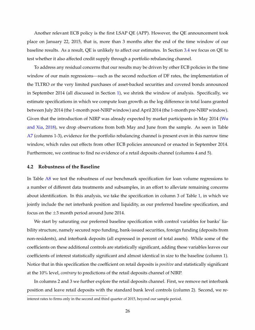
non-residents), and interbank deposits (all expressed in percent of total assets). While some of the

coefficients on these additional controls are statistically significant, adding these variables leaves our

coefficients of interest statistically significant and almost identical in size to the baseline (column 1).

Notice that in this specification the coefficient on retail deposits is positive and statistically significant

at the 10% level, contrary to predictions of the retail deposits channel of NIRP.

In columns 2 and 3 we further explore the retail deposits channel. First, we remove net interbank

position and leave retail deposits with the standard bank level controls (column 2). Second, we re-

interest rates to firms only in the second and third quarter of 2015, beyond our sample period.

26

strict the analysis to large firms (with above-median total assets in March 2014), which makes our

results more directly comparable to Heider et al. (2019), whose sample includes large firms that bor-

row in the syndicated loan market (column 3). In both specifications, the coefficient estimate on retail

deposits is positive and statistically insignificant, which is further evidence against the retail deposits

channel of NIRP.31

Second, we consider the possibility that the announcement of NIRP led to an increase in the

fair value of securities on bank balance sheets (windfall gains) with an associated increase in net

worth, potentially confounding our results. We first note that that lower policy rates benefit both

securities (via prices) and loans (e.g., via a reduction in provisioning, delinquencies and write-offs).

In any case, the evidence we find does not support this concern. We show that the profits of banks

with ex-ante more liquid assets did not improve relatively to other banks in the months after the

NIRP announcement (Table A1). This could be explained by the fact that in Italy, in April 2014, less

than 9% of securities are recorded in the trading portfolio, where unrealized gains and losses from

price fluctuations are recognized in the income statement. Instead, a very large part of the securities

held by banks (more than 40%) are recorded at historic cost. This is consistent with evidence from

Bundesbank data on German banks (Tischer, 2018), and from European Banking Authority stress

testing data for a broad set of European banks (De Marco, 2019).32 However, to further reassure

that that our result on bank liquidity—defined as securities over assets—is not driven by revaluation

gains from the repricing of securities after NIRP, we also explicitly control for a measure of these

gains, which we construct following the approach of Acharya et al. (2019).33 While this measure of

windfall gains is positively correlated with liquidity (the correlation conditional on bank controls

is 0.24), its inclusion in the model does not affect the estimated coefficient on bank liquidity, which

remains positive and significant, and unchanged in size (column 4). An additional argument against

this worry is that our estimates of the impact of NIRP are different from those of policy rate cuts

31In unreported regressions we show that the coefficient of retail deposits is negative and significant only when includedas the only variable in the 3-month window. Simply controlling for bank size makes the estimated coefficient not statisti-cally significant. We further explore the possibility that the retail deposits channel is at work for banks operating in moreconcentrated deposits markets or for banks that ex-ante had lower average deposit rates, finding no robust evidence thatretail deposits matter for the transmission of NIRP to bank lending in Italy.

32Moreover, over the sample period Italian regulations stated that for government bonds recorded at fair value in theavailable-for-sale portfolio, unrealized gains or losses did not impact the regulatory capital. This rule changed in October2016).

33For each security in the bank’s securities portfolio, we calculate the change in price around the NIRP announcement(the difference between the price at end-June 2014 and that at end-April 2014) and multiply these price changes for theholdings of each security outstanding in the bank portfolio before the announcement (end-April 2014). Finally, we addup the individual gains over all the securities in bank portfolios and express them as percent of total equity. Since we alsoknow in which portfolio each security is held, we restrict our analysis to securities held in the marked-to-market portfolios.Further, including the changes in value of the securities recorded at historic costs leaves the results unchanged.

27

above the ZLB, which are similarly associated with windfall gains. More generally, they are different

from results on the role of bank liquidity in the bank lending channel of monetary policy for the U.S.

(e.g., Kashyap and Stein, 2000) and Spain (e.g., Jiménez et al., 2012).

Third, we consider an alternative timing for measuring bank exposure to NIRP. Measuring bank-

level NIRP exposure at end-March 2014 could miss adjustments that banks may have undertaken

ahead of the ECB decision to cut its DF rate to negative levels on June 11, 2014. Given that our

data on interbank market participation are available on a quarterly basis, the only other feasible date

for measuring the net interbank position is end-June 2014. But this is an ex-post measure and may

reflect adjustments that took place between June 11 and June 30, 2014. That said, using end-June 2014

exposure to NIRP in the lending regressions leaves our main results unchanged (column 5).

In column 6 we estimate the baseline specification with Weighted Least Squares (WLS), taking

the logarithm of loan size as weight. The estimates show that the point estimate on the net interbank

position and liquidity are similar to the coefficient estimates in the unweighted (OLS) regressions.

Lastly, we consider alternative timings of NIRP. We start by taking into account the fact that the

pass-through from negative policy rates to overnight interbank rates was not simultaneous: EONIA

turned negative in August. Given that these rates remained positive through most of the period be-

tween June and August 2014, we remove observations for these months and redefine the±3 window

around the period June-August 2014. Column 7 shows that the baseline effects remain statistically

significant and close in magnitude to that of Table 1, column 1. In addition, we account for NIRP

being partly expected the month before its enactment (Wu and Xia, 2018) by re-centering the base-

line analysis on the ±3 months around May and June 2014—and hence dropping the observations

of these months from the sample. Our results are unaffected by the shift of our time window by one

month (column 8).

4.3 NIRP vs. Other Monetary Policy Events

Here we examine the extent to which NIRP differs from conventional and unconventional monetary

policies. For this purpose, we conduct four additional tests which center the period of analysis on

four different monetary policy events. First, we consider the last DF rate cut before NIRP—by 25

basis points to 0% on July 11, 2012. On that occasion, the policy rate cut translated into a decrease

in short-term yields, while the long end of the yield curve remained largely unchanged (Figure 4,

panel a). The second event, in November 2013, is the last cut of the interest rate on the MRO, from

0.50 to 0.25%, before the DF rate went negative. The interest rate on the MRO was the key reference

28

rate before the introduction of negative rates on the deposit facility. In that event, the rate cut did

not flatten the yield curve; if anything, long term yields at end December 2013 increased compared

to September 2013 (see Figure 4, panel b). Third, we examine the announcement of the first LSAP

QE in January 2015. In that event, the yield curve flattened (Figure 4, panel d), as it did after NIRP,

even though the DF rate remained unchanged at −0.20%.34 Fourth, we test whether the portfolio

rebalancing channel is unique to the introduction of negative rates or, instead, persists after further

rate cuts into negative territory. For this purpose, we focus on the most recent episode of monetary

easing:35 in March 2016 the ECB further cut the DF rate to -0.40 basis points. This episode was

associated with a further, smaller, flattening of the yield curve (Figure 4, panel e).36

The regression results for these tests are reported in Table 2.37 We find that during the previous

rate cuts in positive territory (the first two events discussed above), the impact of monetary policy

is very different from our findings for NIRP. For the July 2012 DF rate cut, the coefficients of net

interbank position and liquidity are both negative and statistically significant. Liquidity yields a

negative and significant coefficient (for the±3 month window) after the reduction of the interest rate

on the MRO as well. These results are consistent with the standard bank lending channel of monetary

policy (Kashyap and Stein, 2000; Jiménez et al., 2012), according to which a monetary easing has

stronger effects for banks with an ex-ante lower liquidity buffer (i.e., less need of an ease of monetary

policy for banks with higher liquidity as these banks need less extra liquidity to continue lending).

By contrast, after the QE (LSAP) announcement, we find that more liquid banks expand credit

supply.38 However, the coefficient of net interbank position is smaller than for NIRP and statistically

insignificant. This result is not surprising given that QE is not associated with a drop in short-term

policy rates.

34Gambetti and Musso (2017) also find that the QE announcement in January 2015 was accompanied by a flatteningof the yield curve. The authors explain that the announcement was to some extent expected. However, they also reportthat according to market polls and anecdotal evidence from newspapers, the large scope of asset purchases was not fullyexpected and hence did surprise the markets.

35This is the last episode of monetary easing before the September 2019 rate cut, which we cannot yet analyze.36In the press release that announced the cut of interest rate to -0.30 on December 3, 2015 there is also the announcement

of an extension of the APP programme. Since analysts expected a much larger extension of the monthly purchases ofsecurities under the APP programme there was a strong negative reaction in the market on the day of the announcement:the DAX and the CAC 30 lost 3.6% and the Euro appreciated 3% against the US Dollar. This presence of confoundinginformation makes this event less suitable for the identification of the NIRP impact.

37Similar to the baseline regressions, we analyze the impact of other monetary policy announcements on bank creditsupply in the ±3 (panel A) and ±6 (panel B) month windows around these dates. We measure banks’ net interbankposition and liquidity, in the last available date before the policy announcements, that is, in June 2012, September 2013,December 2014, and December 2015, respectively.

38This is consistent with the results in Rodnyansky and Darmouni (2017) and Albertazzi et al. (2018). These papers showthat, both in the U.S. and in the euro area, those banks that benefitted more from QE lent more to firms.

29

Finally, the effect of the March 2016 interest rate cut is similar to that of the NIRP introduction.

The result suggests that the portfolio rebalancing channel is not a one-off effect due to the break

through the ZLB, but rather the result of the flattening of the yield curve, which was also achieved,

albeit to a smaller extent, in the March 2016 rate cut as well. In unreported regressions, we continue

to find no evidence of a contractionary retail deposits channel for the March 2016 event. These results

alleviate possible concerns that our baseline finding was caused by rates not being “low enough” or

low “for long enough” to dampen bank profitability. In other words, this evidence would suggest

that the reversal rate (Brunnermeier and Koby, 2018) has not yet been reached. Even with the DF

rate at -0.40% and negative rates in place for almost two years, there is evidence of an expansionary

portfolio rebalancing channel and no sign of a contractionary retail deposits channel, similar to the

initial DF rate cut in mid-2014 (column 4 of Table 2).39

Taken together, our tests suggest that the NIRP announcement, as well as later cuts below zero, ac-

tivate a portfolio rebalancing mechanism. Banks rebalance their portfolios from liquid assets towards

credit supply. This rebalancing behavior is not at play after policy rate cuts in positive territory and

close to the ZLB. By contrast, the QE announcement generates effects that are similar to NIRP (in the

sense of portfolio rebalancing, but with differences across exposure variables in their suitability to

capture the transmission mechanism).

4.4 Falsification Tests

An important identifying assumption in our empirical framework is “parallel trends,” which would

be violated if our NIRP bank exposure variables were correlated with pre-NIRP loan growth. To

rule out pre-existing trends in loan growth for banks with different net interbank and liquidity posi-

tions, we run regressions that are similar to our baseline specification (Table 1, column 3), but center

the ±3 and ±6 month windows on different months before the NIRP announcement. The results are

reported in Table A9, which shows the estimated coefficients of the net interbank position and liquid-

ity (both measured at end-March 2014). The top panel considers the ±3 months window and reports

results centered on December 2013, January 2014, and February 2014, the last month for which the

post-NIRP 3-month window does not include June 2014 (November 2013-May 2014). For the same

reason, the bottom panel reports results for the ±6 month window around September, October, and

November 2013. The results indicate that the parallel trends assumption is valid given that the coef-

39The estimated coefficients for the portfolio rebalancing are larger in 2016 but the standard deviations of the variablesare smaller.

30

ficients estimated in the months before NIRP are generally close to zero and statistically insignificant.

4.5 NIRP and Portfolio Rebalancing Across Euro Area Banks

A residual concern is related to our analysis being based on Italian banks. One could argue that the

effect of negative rates may be heterogeneous across the euro area. Differences in deposit rates across

banks in different countries, for instance, may make the retail deposits channel more or less effective.

Similarly, differences in sovereign risk premia may make the reversal rate (Brunnermeier and Koby,

2018) country-specific, so that negative rates are contractionary in some countries, but expansionary

in others. To address these concerns, we replicate our baseline analysis in a large panel of euro area

banks. The benefit of examining the effect of NIRP across countries comes at the cost of a weaker

identification strategy, as with bank-level data, we can neither analyze loan level volumes and prices

nor we can properly control for firm-level credit demand with borrower fixed effects.

We collect yearly data on bank balance sheet data from Fitch Connect, for the period 2010 to

2016. After dropping duplicates and cleaning the data (we winsorize all variables at the 1st and

99th percentile), the sample includes 1,838 commercial banks. Using this (unbalanced) sample at the

bank-year level, we estimate the following equation:

∆Loanbt = α0 Liquiditybt + α1 Liquiditybt × Post NIRPt + (3)

β0 Retail depositsbt + β1 Retail depositsbt × Post NIRPt + γ′Xbt + φb + τt + εbt,

where ∆Loanbt is the change in the ratio of gross loans over total assets between t + 1 and t. Liquidity

and retail deposits are defined as in the main analysis and scaled by total assets. By contrast, data

limitations prevent us from computing a measure of exposure to the short-term interbank market. As

a result, the two key variable of interests are the interactions of liquidity and retail deposits with the

Post-NIRP dummy (equal to 1 starting at the introduction of NIRP). The coefficients α1 and β1 test

for the portfolio rebalancing and the retail deposits channels, respectively. The set of bank controls

(Xbt) mimics as much as possible the main analysis and includes: the ratio of gross loans over assets,

equity over assets, the logarithm of total assets, return on assets, and the ratio of NPLs over gross

loans. All these variables are included as stand-alone controls and interacted with the Post-NIRP

dummy. The model also includes bank (φb) and year (τt) fixed effects. Standard errors are clustered

at the bank level.

The results are shown in Table 4, which reports the coefficients of the key interaction terms. The

31

first two columns do not include NPLs as a control variable to maximize sample size, while columns

2 and 4 include a triple interaction with GIIPS countries (Greece, Ireland, Italy, Portugal and Spain) to

test for differential lending behavior in response to NIRP. The results in this table confirm our main

findings (based on loan-level data) for Italy in a significantly larger sample of European banks. The

estimates consistently show that more liquid banks expand lending more after NIRP, even until 2016,

with no significant differences between the core and the periphery of the euro area. By contrast, we

do not find any evidence that banks more dependent on retail deposits change their lending after the

introduction of negative rates. These results also confirm what found by Demiralp et al. (2019) on a

sample of euro area banks.

4.6 Heterogeneity: Firm Risk and Size

Thus far, our findings show that NIRP-affected banks rebalance portfolios away from liquid assets to

bank loans. It is important to understand whether banks further rebalance within the loan portfolio,

in other words whether credit increases homogeneously across firms, or whether it does so more

towards certain types of firms.

We focus on two key firm dimensions—riskiness and size—which are relevant for the following

reasons. First, riskier and smaller firms are typically more credit constrained and monetary easing

should lead banks to expand credit towards marginal, financially-constrained borrowers, too. Sec-

ond, we would like to pin down the channel driving our results more precisely. If banks rebalance

their portfolios towards higher yielding assets, they should expand credit especially towards higher

yielding loans. Riskiness and size are good proxies for the yield banks can extract from borrowers

because risky and small borrowers are typically charged higher loan spreads and have fewer oppor-

tunities to substitute across lenders. We split the sample between (ex-ante) small and large firms, and

firms with (ex-ante) weak and strong credit ratings, around the median of the distribution of total

assets and that of the Altman z-score respectively (at end-2013).

The results are shown in Table 3, where the first three columns refer to the ±3 month window

and the last three columns to the ±6 month window. We are testing whether the expansion of credit

is stronger for certain type of firms, therefore we include bank fixed effects in all the specifications to

absorb unobserved bank heterogeneity and focus on the interaction terms between firm characteris-

tics and the banks’ net interbank position and liquidity, respectively. The results consistently show

that the relative expansion of credit supply by more NIRP-exposed banks, measured either by the

net interbank position (panel A) or by the liquidity ratio (panel B), is significantly higher for ex-ante

32

riskier firms (with high z-score or low credit rating) and smaller firms.

Note that the increase in ex-ante risk-taking by more NIRP-affected banks does not translate into

higher levels of ex-post NPLs, even five years after the introduction of NIRP. In Table A10 we report

bank-level regressions where the dependent variable is the change in the NPL ratio over one year

(top panel) and five years (bottom panel) after the introduction of NIRP and the regressors are bank

characteristics at end-March 2014. The results show that more NIRP-exposed banks do not experience

a steeper deterioration in loan quality (despite higher lending, and to ex-ante riskier firms), which

suggests that banks do not engage in “excessive” risk-taking, but extend loans to ex-ante riskier yet

viable firms.40

Finally, we explore the possibility that banks more reliant on retail deposits, even though they

do not contract lending, concentrate their lending on riskier firms, as found by Heider et al. (2019).

The results—reported in panel C—do not show any significant and robust difference in lending to

risky firms across banks with different levels of retail deposits. The coefficient of the interaction term

between retail deposits and risky firms is marginally significant (at 10% level), but only for the ±3

month window.

4.7 Transmission to Loan Rates

Our analysis so far has focused on the impact of NIRP on bank loan volume decisions. But another

margin of adjustment is pricing. Eggertsson et al. (2019) use bank-level data and variation in the

share of deposit funding across Swedish banks to document a weaker pass-through from the policy

rate to loan rates during the NIRP period. By contrast, using loan-level data, we compare the change

in the interest rates on loans granted to the same firm by at least two banks with different exposure

to the policy, before and after NIRP introduction. Documenting a strong pass-through of negative

policy rates to bank loan rates in our approach would further strengthen a supply-side interpretation

of the impact of NIRP on bank credit.

Table 5 reports the estimates for net loan rates, separating credit lines and overdraft facilities

from term loans. Across columns, our results indicate that negative policy rates affect lending rates

through banks’ net interbank position and the broader measure of liquidity, although the effect is

stronger on credit lines and overdraft facilities than on term loans, as expected. Using the estimates

40Another potential source of heterogeneity is bank capital, as banks with lower capital ratios may be constrained inrebalancing their portfolio toward more credit. In unreported regressions, we test whether banks’ responses to the intro-duction of NIRP varies with the level of ex-ante bank capital. We find some weak evidence that the effect of NIRP on thecredit supply is larger for high-capital banks, but the results are not robust.

33

in column 3, a change in one standard deviation in the banks’ net interbank position (liquidity) leads

to 29 bps (29 bps) reduction of loan rates on credit lines and overdraft facilities after 6 months; this

effect is economically meaningful, as it corresponds to almost a 4% reduction (the median net loan

rate in 7.9%). In the case of term loans, these effects are smaller and limited to about 5 bps, which

correspond to a 1.3% reduction of loan rates after 6 months.

We find qualitatively similar results for gross interest rates, which capture the total cost of bor-

rowing. In this case, the size of the effects on credit lines and overdraft facilities are even larger. A

one standard deviation change in the banks’ net interbank position (liquidity) leads to 89 bps (62 bps)

reduction of loan rates after 6 months, which corresponds to a 7.6% (5.4%) reduction of gross rates

on credit lines and overdraft facilities (Table A11).

Finally, our results are robust to controlling for banks’ reliance on retail deposits and show no

evidence that NIRP affects loans rates through the retail deposits channel (column 4). Hence, the

retail deposits channel is inactive both in lending volumes and loan rates, measured either in net or

gross terms.

5 Real Effects

Our analysis of credit register lending data shows that NIRP-exposed banks increase credit supply in

response to NIRP. But did this positive effect on credit translate into better outcomes in the real sec-

tor? To answer this question, we estimate firm-level regressions where the dependent variable is the

growth rate of total firm-level credit in the ±6 month window around June 2014. The net interbank

position and liquidity are defined at the firm level as the average net position in the interbank market

and average liquidity ratio of the firms’ lenders in March 2014, weighted by the share of total credit

granted to the firm by each lender. We control for the same (weighted) bank characteristics as in

the loan-level baseline regressions, a set of firm characteristics (size, riskiness and return on assets),

firm-level demand (measured as the estimated firm fixed effects from the firm-bank loan-growth

regressions), and location and industry fixed effects.

The results—reported in the first column of Table 6—show that the coefficients on the net inter-

bank position and liquidity are positive and statistically significant, both in the sample of manufac-

turing firms (panel A) and in the full sample of manufacturing and services firms (panel B). Using

the estimates for the full sample, we find that a one standard deviation change in a firm’s lenders’ net

interbank position (liquidity) is associated with a 2.4 (1.0) percentage point increase in total credit for

34

that firm. These effects are economically large given that the average change in total firm-level credit

in the ±6 month window is 1.7%.

Next, we determine whether more credit translates into stronger firm performance. In the remain-

ing columns of Table 6 we use the same specification but consider the following firm outcomes: the

growth rate of fixed assets (investment expenditure, column 2) and the growth of total payroll (wage

bill, column 3), which are key components of aggregate output. In the sample of manufacturing

firms (panel A) we find that firms borrowing from lenders with greater exposure to NIRP (prior to

the NIRP introduction) expand economic activity relatively more. Looking at the coefficient estimate

for the net interbank position, firm investment increases by 6.8 percentage points and the wage bill

by 3.8 percentage points more for firms borrowing from banks with (one standard deviation) larger

ex-ante net interbank position. Similarly, a one standard deviation increase in banks’ ex-ante liquid-

ity is associated with a 4.6 percentage points increase in firm investment and with 1 percentage point

increase in the wage bill in response to NIRP.41

6 Conclusions

Despite the importance of negative interest rates for our broader understanding of finance and macroe-

conomics, systematic evidence on their transmission to the economy through the banking system re-

mains scarce. Not only do several major economies (such as the euro area and Japan) currently have

negative policy rates and a significant share of global debt trades at negative yields, but NIRP may

become even more center-stage in the future given the current low interest rate environment.

We study the impact of NIRP exploiting the introduction of negative nominal policy rates by the

ECB in mid-2014, as well as other rate cuts, and comprehensive administrative microdata from Italy.

Our main contribution to the literature is to document that NIPR has expansionary effects, and yet

differs from policy rate cuts just above the ZLB. The mechanism by which NIRP works is to shift

down and flatten the yield curve, thereby incentivizing banks to rebalance their portfolio from liquid

assets to lending—a portfolio rebalancing channel. Furthermore, we show that the bank lending

channel of NIRP is different from the traditional channel associated with interest rate cuts above the

ZLB (Kashyap and Stein, 1995, 2000; Jiménez et al., 2012; Drechsler et al., 2017). We find no evidence

of a retail deposits channel (unlike Eggertsson et al. (2019) and Heider et al. (2019)) for loan volumes,

rates, or bank risk-taking, even after ECB’s last rate cut.

41Results for wage bill growth are similar in the full sample of firms (panel B). This is not the case for investment, asmanufacturing firms arguably are more dependent on credit to finance fixed assets.

35

Our main results are as follows. First, we document an increase in the growth rate of total bank

credit after the introduction of NIRP with aggregate time-series data. Second, we use loan-level

volume and price data to show that NIRP has expansionary effects on credit supply and the real

economy through the portfolio rebalancing channel. Differently from previous rate cuts just above

the ZLB, the announcement of NIRP shifted down and flattened the entire yield curve, widening the

wedge between yields on safer, liquid assets and yields on riskier assets, such as corporate loans. The

same portfolio rebalancing channel is also active after ECB’s last rate cut (with available data) in 2016,

which went further into negative territory. To further substantiate our findings, we take our analysis

to a cross-country setting and show that (ex-ante) more liquid euro area banks also increase credit

more than other banks after the introduction of NIRP. Moreover, we show that more NIRP-affected

banks expand credit supply more to ex-ante riskier and smaller firms, and cut loan rates, thereby

inducing sizable firm-level real effects, including on investment and wage bill, without higher ex-

post delinquencies.

36

References

Acharya, V., Eisert, T., Eufinger, C., and Hirsch, C. (2019). Whatever it Takes: The Real Effects ofUnconventional Monetary Policy. Review of Financial Studies, 32(9):3366–3411.

Acharya, V. V. and Merrouche, O. (2012). Precautionary Hoarding of Liquidity and Interbank Mar-kets: Evidence from the Subprime Crisis. Review of Finance, 17(1):107–160.

Acharya, V. V., Pierret, D., and Steffen, S. (2016). Lender of Last Resort versus Buyer of Last Resort:Evidence from the European Sovereign Debt Crisis. mimeo. New York University.

Adrian, T. and Shin, H. S. (2010). Financial Intermediaries and Monetary Economics. In Friedman,B. M. and Woodford, M., editors, Handbook of Monetary Economics, volume 3a, chapter 12, pages601–650. Elsevier.

Albertazzi, U., Becker, B., and Boucinha, M. (2018). Portfolio rebalancing and the transmission oflarge-scale asset programmes: evidence from the euro area. Working Paper 2125, European CentralBank.

Allen, F. and Rogoff, K. S. (2011). Asset Prices, Financial Stability and Monetary Policy. In Jansson,P. and Persson, M., editors, The Riksbank’s Inquiry into the Risks in the Swedish Housing Market, pages189–218. Sveriges Riksbank, Stockholm.

Altavilla, C., Boucinha, M., and Peydró, J.-L. (2018). Monetary policy and bank profitability in a lowinterest rate environment. Economic Policy, 33(96):531–586.

Altavilla, C., Burlon, L., Giannetti, M., and Holton, S. (2019). Is there a zero lower bound? The effectsof negative policy rates on banks and firms. ECB Working Paper 2289, European Central Bank,Frankfurt.

Altavilla, C., Carboni, G., and Motto, R. (2015). Asset purchase programmes and financial markets:lessons from the euro area. Working Paper 1864, European Central Bank.

Altman, E. I. (1968). Financial ratios, discriminant analysis and the prediction of corporatebankruptcy. The Journal of Finance, 23(4):589–609.

Angelini, P., Nobili, A., and Picillo, C. (2011). The Interbank Market after August 2007: What HasChanged, and Why? Journal of Money, Credit and Banking, 43(5):923–958.

Arce, O., Garcia-Posada, M., Mayordomo, S., and Ongena, S. (2018). Adapting lend-ing policies when negative interest rates hit banks’ profits. Electronic copy available at:https://ssrn.com/abstract=3161924.

Arseneau, D. M. (2017). How Would US Banks Fare in a Negative Interest Rate Environment? Financeand Economics Discussion Series 2017-030, Federal Reserve Board.

Arteta, C., Kose, A., Stocker, M., and Taskin, T. (2018). Implications of negative interest rate policies:An early assessment. Pacific Economic Review, 23(1):8–26.

Baldo, L., Hallinger, B., Helmus, C., Herrala, N., Martins, D., Mohing, F., Petroulakis, F., Resinek, M.,Vergote, O., Usciati, B., et al. (2017). The distribution of excess liquidity in the euro area. OccasionalPaper 200, European Central Bank, Frankfurt.

Basten, C. and Mariathasan, M. (2018). How Banks Respond to Negative Interest Rates: Evidencefrom the Swiss Exemption Threshold. CESifo Working Paper 6901, CESifo, Munich.

37

Benetton, M. and Fantino, D. (2018). Competition and The Pass-Through of Unconventional Mone-tary Policy: Evidence from TLTROs. unpublished working paper.

Bernanke, B. S. (2016). Modifying the Fed’s policy framework: Does a higher inflation target beatnegative interest rates? Brookings.

Bernanke, B. S. (2017). Monetary Policy in a New Era. Prepared for conference on Rethinking Macroe-conomic Policy, Peterson Institute.

Bhattarai, S. and Neely, C. (2016). A Survey of the Empirical Literature on U.S. UnconventionalMonetary Policy. Working Paper 2016-021, Federal Reserve Bank of St. Louis.

Bofondi, M., Carpinelli, L., and Sette, E. (2018). Credit Supply During a Sovereign Debt Crisis. Journalof the European Economic Association, 16(3):696–729.

Borio, C. and Zhu, H. (2012). Capital regulation, risk-taking and monetary policy: A missing link inthe transmission mechanism? Journal of Financial Stability, 8(4):236–251.

Brunnermeier, M. K. and Koby, Y. (2018). The reversal interest rate: An effective lower bound onmonetary policy. Mimeo. Princeton University.

Chakraborty, I., Goldstein, I., and MacKinlay, A. (2019). Monetary Stimulus and Bank Lending.Journal of Financial Economics, forthcoming.

Chodorow-Reich, G. (2014). Effects of unconventional monetary policy on financial institutions.Brookings Papers on Economic Activity, Spring(1):155–227.

Christensen, J. H. (2019). Yield Curve Responses to Introducing Negative Policy Rates. FRBSF Eco-nomic Letter 27, Federal Reserve Bank of San Francisco, San Francisco.

Cingano, F., Manaresi, F., and Sette, E. (2016). Does Credit Crunch Investments Down? New Evidenceon the Real Effects of the Bank-Lending Channel. Review of Financial Studies, 29(10):2737–2773.

Cœuré, B. (2016). Assessing the implications of negative interest rates. Speech at the Yale FinancialCrisis Forum, Yale School of Management, New Haven.

Cœuré, B. (2017). Dissecting the yield curve: a central bank perspective. Welcome remarks at theannual meeting of the ECB’s Bond Market Contact Group. Frankfurt am Main.

Curdia, V. and Woodford, M. (2011). The Central-Bank Balance Sheet as an Instrument of MonetaryPolicy. Journal of Monetary Economics, 58(1):54–79.

D‘Amico, S. and King, T. B. (2013). Flow and stock effects of large-scale treasury purchases: Evidenceon the importance of local supply. Journal of Financial Economics, 108(2):425–448.

De Marco, F. (2019). Bank lending and the european sovereign debt crisis. Journal of Financial andQuantitative Analysis, 54(1):155–182.

Debortoli, D., Galí, J., and Gambetti, L. (2019). On the Empirical (Ir)Relevance of the Zero LowerBound Constraint. In Eichenbaum, M. S., Hurst, E., and Parker, J. A., editors, NBER MacroeconomicsAnnual 2019, volume 34. University of Chicago Press.

Dell’Ariccia, G., Laeven, L., and Suarez, G. A. (2017). Bank Leverage and Monetary Policy’s Risk-Taking Channel: Evidence from the United States. Journal of Finance, 72(2):613–654.

Dell’Ariccia, G., Rabanal, P., and Sandri, D. (2018). Unconventional Monetary Policies in the EuroArea, Japan, and the United Kingdom. Journal of Economic Perspectives, 32(4):147–172.

38

Demiralp, S., Eisenschmidt, J., and Vlassopoulos, T. (2019). Negative interest rates, excess liquidityand retail deposits: Banks’ reaction to unconventional monetary policy in the euro area. ECBWorking Paper 2283, European Central Bank.

Draghi, M. (2016). Press conference introductory statement. Introductory statement at ECB PressConference, Frankfurt am Main, March 10, 2016.

Draghi, M. (2017). Press conference introductory statement. Introductory statement at ECB PressConference, Frankfurt am Main, April 27, 2017.

Drechsler, I., Savov, A., and Schnabl, P. (2017). The deposits channel of monetary policy. The QuarterlyJournal of Economics, 132(4):1819–1876.

Drechsler, I., Savov, A., and Schnabl, P. (2018). Banking on Deposits: Maturity Transformation with-out Interest Rate Risk. NBER Working Paper 24582, National Bureau of Economic Research.

ECB (2016). Financial stability review. Technical report, European Central Bank.Eggertsson, G. B., Juelsrud, R. E., Summers, L. H., and Wold, E. G. (2019). Negative Nominal Interest

Rates and the Bank Lending Channel. NBER Working Paper 25416, National Bureau of EconomicResearch.

Eisenschmidt, J. and Smets, F. (2017). Negative interest rates: Lessons from the euro area. unpub-lished working paper.

Eser, F., Lemke, W., Nyholm, K., Radde, S., and Vladu, A. L. (2019). Tracing the impact of the ECB’sasset purchase programme on the yield curve. Working Paper Series 2293, European Central Bank.

Gambetti, L. and Musso, A. (2017). The macroeconomic impact of the ECB’s expanded asset purchaseprogramme (APP). Working Paper 2075, European Central Bank, Frankfurt.

Gertler, M. and Karadi, P. (2011). A Model of Unconventional Monetary Policy. Journal of MonetaryEconomics, 58(1):17–34.

Grisse, C., Krogstrup, S., and Schumachera, S. (2017). Lower-Bound Beliefs and Long-Term InterestRates. International Journal of Central Banking, 13(3):165–202.

Heider, F., Saidi, F., and Schepens, G. (2019). Life Below Zero: Bank Lending Under Negative PolicyRates. Review of Financial Studies, 32(10):3728–3761.

Hutchinson, J. and Smets, F. (2017). Monetary Policy in Uncertain Times: ECB Monetary Policy SinceJune 2014. The Manchester School, 85(52):c1–c15.

Imbens, G. W. and Wooldridge, J. M. (2009). Recent developments in the econometrics of programevaluation. Journal of Economic Literature, 47(1):5–86.

IMF (2016). Euro Area Policies–Selected Issues. Technical report, International Monetary Fund, Wash-ington DC. IMF Country Report No. 16/220.

IMF (2017). Negative Interest Rate Policies–Initial Experiences and Assessments. Technical report,International Monetary Fund, Washington DC. IMF Policy Paper.

Iyer, R., Lopes, S., Peydro, J., and Schoar, A. (2014). Interbank liquidity crunch and the firm creditcrunch: Evidence from the 2007-2009 crisis. Review of Financial Studies, 27(1):347–372.

Jiménez, G., Mian, A. R., Peydró, J.-L., and Saurina, J. (2019). The Real Effects Of The Bank LendingChannel. Journal of Monetary Economics, Forthcoming.

39

Jiménez, G., Ongena, S., Peydró, J., and Saurina, J. (2012). Credit supply and monetary policy:Identifying the bank-balance sheet channel with loan applications. American Economic Review,102(5):2121–2165.

Jiménez, G., Ongena, S., Peydró, J., and Saurina, J. (2014). Hazardous times for monetary policy:What do twenty-three million bank loans say about the effects of monetary policy on credit risk?Econometrica, 2(82):463–505.

Jiménez, G., Ongena, S., Peydró, J.-L., and Saurina, J. (2017). Macroprudential Policy, Countercycli-cal Bank Capital Buffers, and Credit Supply: Evidence from the Spanish Dynamic ProvisioningExperiments. Journal of Political Economy, 125(6):2126–2177.

Kashyap, A. K. and Stein, J. C. (1995). The impact of monetary policy on bank balance sheets. InCarnegie-Rochester Conference Series on Public Policy, volume 42, pages 151–195. Elsevier.

Kashyap, A. K. and Stein, J. C. (2000). What do a million observations on banks say about the trans-mission of monetary policy? American Economic Review, pages 407–428.

Khwaja, A. I. and Mian, A. (2008). Tracing the impact of bank liquidity shocks: Evidence from anemerging market. American Economic Review, 98(4):1413–42.

Krishnamurthy, A. and Vissing-Jorgensen, A. (2011). The Effects of Quantitative Easing on InterestRates: Channels and Implications for Policy. Brookings Papers on Economic Activity, Fall(2):215–265.

Lemke, W. and Vladu, A. (2017). Below the zero lower bound: A shadow-rate term structure modelfor the euro area. ECB Working Paper 1991, European Central Bank.

Lopez, J. A., Rose, A. K., and Spiegel, M. M. (2018). Why Have Negative Nominal Interest RatesHad Such a Small Effect on Bank Performance? Cross Country Evidence. Working Paper 2018-07,Federal Reserve Bank of San Francisco.

Madaschi, C. and Pablos Nuevos, I. (2017). The profitability of banks in a context of negative mone-tary policy rates: The cases of Sweden and Denmark. ECB Occasional Paper 195, European CentralBank.

Martinez-Miera, D. and Repullo, R. (2017). Search for yield. Econometrica, 85(2):351–378.McKay, A., Nakamura, E., and Steinsson, J. (2016). The power of forward guidance revisited. The

American Economic Review, 106(10):3133–3158.Nakamura, E. and Steinsson, J. (2018). Identification in macroeconomics. Journal of Economic Perspec-

tives, 32(3):59–86.Peydró, J.-L., Polo, A., and Sette, E. (2017). Monetary policy at work: Security and credit application

registers evidence. mimeo. Universitat Pompeu Fabra.Rajan, R. G. (2005). Has Financial Development Made the World Riskier? In Proceedings - Economic

Policy Symposium - Jackson Hole, Federal Reserve Bank of Kansas City, pages 313–369.Rodnyansky, A. and Darmouni, O. M. (2017). The Effects of Quantitative Easing on Bank Lending

Behavior. The Review of Financial Studies, 30(11):3858–3887.Rognlie, M. (2016). What Lower Bound? Monetary Policy with Negative Interest Rates. unpublished

working paper.Rogoff, K. (2017). Dealing with Monetary Paralysis at the Zero Bound. Journal of Economic Perspectives,

40

31(3):47–66.Rogoff, K. S. (2016). The Curse of Cash. University Press, Princeton.Rostagno, M., Bindseil, U., Kamps, A., Lemke, W., Sugo, A., and Vlassopoulos, T. (2016). Breaking

through the zero line: The ECB’s negative interest rate policy. Presentation at Brookings.Ruge-Murcia, F. J. (2006). The expectations hypothesis of the term structure when interest rates are

close to zero. Journal of Monetary Economics, 53(7):1409–1424.Sette, E. and Gobbi, G. (2015). Relationshio Lending During a Financial Crisis. Journal of the European

Economic Association, 13(3):453–481.Sims, E. and Wu, J. C. (2019). Evaluating Central Banks’ Tool Kit: Past, Present, and Future. NBER

Working Paper 26040, National Bureau of Economic Research.Stein, J. C. (2013). Overheating in Credit Markets: Origins, Measurement, and Policy Responses.

Speech at the “Restoring Household Financial Stability after the Great Recession: Why HouseholdBalance Sheets Matter” research symposium sponsored by the St. Louis Fed.

Swanson, E. T. (2018). The Federal Reserve Is Not Very Constrained by the Lower Bound on NominalInterest Rates. Brookings Papers on Economic Activity, 2018(Fall):555–572.

Taylor, J. B. (2009). Economic Policy and the Financial Crisis: An Empirical Analysis of What WentWrong. Critical Review, 21(2-3):341–364.

Tischer, J. (2018). Quantitative easing, portfolio rebalancing and credit growth: Micro evidence fromGermany. Discussion Paper 20/2018, Deutsche Bundesbank.

Turk, R. A. (2016). Negative Interest Rates: How Big a Challenge for Large Danish and SwedishBanks? IMF Working Paper 16/198, International Monetary Fund, Washington DC.

Ulate, M. (2019). Going Negative at the Zero Lower Bound: The Effects of Negative Nominal InterestRates. Working paper, Federal Reserve Bank of San Francisco.

Upper, C. (2006). Contagion Due to Interbank Credit Exposures: What Do We Know, Why Do WeKnow It, and What Should We Know? BIS Working Paper.

Wu, J. C. and Xia, F. D. (2018). Negative Interest Rate Policy and Yield Curve. NBER Working Paper25180, National Bureau of Economic Research.

Zimmermann, K. (2019). Monetary Policy and Bank Profitability, 1870 – 2015. Available at SSRN:https://ssrn.com/abstract=3322331.

41

Figures and Tables

Figure 1: Policy and Interbank Rates, January 2014–December 2014

ECB

intro

duct

ion

of N

IRP

(-0.1

0%)

-.3

-.2

-.1

0

.1

.2

.3

Inte

rest

rate

s (e

nd p

erio

d)

2014

m1

2014

m2

2014

m3

2014

m4

2014

m5

2014

m6

2014

m7

2014

m8

2014

m9

2014

m10

2014

m11

2014

m12

Deposit facility Euribor, 1 week

Notes: The chart plots the ECB Deposit Facility rate and the Euribor one-week interest rate, at monthly frequency, taking the end-monthvalues. The solid vertical line corresponds to end June 2014, and separates the pre-NIRP (January 2014–June 2014) from the post-NIRP(July 2014–December 2014) windows. Source: Thomson Reuters Eikon.

42

Figure 2: Forward Curves with Negative Policy Rates

0

.5

1

1.5

1M 2M 3M 6M 9M 1Y1Y

3M

1Y 6

M1Y

9M 2Y

2Y 3

M2Y

6M

2Y 9

M 3Y3Y

3M

3Y 6

M3Y

9M 4Y

4Y 3

M4Y

6M

4Y 9

M 5Y5Y

3M

5Y 6

M5Y

9M 6Y

6Y 3

M6Y

6M

6Y 9

M 7Y7Y

3M

7Y 6

M7Y

9M 8Y

End of April 2014 End of July 2014

Notes: The charts plot yield curves before and after the ECB introduction of negative policy rates in June 2014. Source: Thomson ReutersEikon.

Figure 3: Aggregate Credit Growth to Non-Financial Corporations in Italy, 2014

-5

-4

-3

-2

Cre

dit g

row

th (y

ear-o

n-ye

ar)

2014

m1

2014

m2

2014

m3

2014

m4

2014

m5

2014

m6

2014

m7

2014

m8

2014

m9

2014

m10

2014

m11

2014

m12

Notes: The chart plots the year-on-year growth rate of total bank credit to non-financial corporations. Source: Bank of Italy.

43

Figure 4: Forward Curves with Conventional and Unconventional Monetary Policy

0

.5

1

1M 2M 3M 6M 9M 1Y1Y

3M

1Y 6

M1Y

9M 2Y

2Y 3

M2Y

6M

2Y 9

M 3Y3Y

3M

3Y 6

M3Y

9M 4Y

4Y 3

M4Y

6M

4Y 9

M 5Y5Y

3M

5Y 6

M5Y

9M 6Y

6Y 3

M6Y

6M

6Y 9

M 7Y7Y

3M

7Y 6

M7Y

9M 8Y

End of May 2012 End of August 2012

(a) July 2012 (DF rate cut in positive territory)

0

.5

1

1.5

1M 2M 3M 6M 9M 1Y1Y

3M

1Y 6

M1Y

9M 2Y

2Y 3

M2Y

6M

2Y 9

M 3Y3Y

3M

3Y 6

M3Y

9M 4Y

4Y 3

M4Y

6M

4Y 9

M 5Y5Y

3M

5Y 6

M5Y

9M 6Y

6Y 3

M6Y

6M

6Y 9

M 7Y7Y

3M

7Y 6

M7Y

9M 8Y

End of September 2013 End of December 2013

(b) November 2013 (MRO rate cut in positive territory)

-.2

0

.2

.4

.6

1M 2M 3M 6M 9M 1Y1Y

3M

1Y 6

M1Y

9M 2Y

2Y 3

M2Y

6M

2Y 9

M 3Y3Y

3M

3Y 6

M3Y

9M 4Y

4Y 3

M4Y

6M

4Y 9

M 5Y5Y

3M

5Y 6

M5Y

9M 6Y

6Y 3

M6Y

6M

6Y 9

M 7Y7Y

3M

7Y 6

M7Y

9M 8Y

End of November 2014 End of February 2015

(c) Jan. 2015 (QE (APP))

-.4

-.2

0

.2

.4

1M 2M 3M 6M 9M 1Y1Y

3M

1Y 6

M1Y

9M 2Y

2Y 3

M2Y

6M

2Y 9

M 3Y3Y

3M

3Y 6

M3Y

9M 4Y

4Y 3

M4Y

6M

4Y 9

M 5Y5Y

3M

5Y 6

M5Y

9M 6Y

6Y 3

M6Y

6M

6Y 9

M 7Y7Y

3M

7Y 6

M7Y

9M 8Y

End of January 2016 End of April 2016

(d) March 2016 (last DF rate cut in negative territory)

Notes: The charts plot the yield curves before and after: the ECB DF rate cut of July 2012 (panel a), the ECB MRO rate cut of November2013 (panel b), the ECB announcement of QE (expanded asset purchase programme) in January 2015 (panel c), and the ECB interest ratecut of March 2016 (panel d). Source: Thomson Reuters Eikon.

44

Figure 5: Negative Policy Rates and the Wedge Between Yields on Safer and Riskier Assets

ECB

1st d

ecis

ion

on N

IRP

-.02

0

.02

.04

.06

Diff

eren

ce in

yie

lds

(per

cent

)

2014m2 2014m3 2014m4 2014m5 2014m6 2014m7 2014m8

Notes: The chart plots the growth rate of the difference (“wedge”) between the average yield on loans to Italian non-financial corporationsand that on Italian government bonds, expressed in percent and normalized at 0 in May 2014. Data on market expectations show that theintroduction of NIRP in June 2014 was partly expected in May 2014 (Wu and Xia, 2018). Source: European Central Bank statistical datawarehouse and Thomson Reuters Eikon.

45

Table 1: Negative Policy Rates and Bank Credit Supply—Baseline regressions

Notes: The table presents OLS estimates of model 1. The dependent variable is loan growth at the bank-firm-month level, calculated aslog difference between the post- and the pre-NIRP period. The length of the pre- and post-NIRP periods ranges between 3 and 6 months,centered around June 2014, which is excluded from the sample. Net interbank position is measured by the ratio of interbank loans minusinterbank deposits with maturity up to one week, over total assets, as of end-March 2014. Liquidity is the ratio of securities over totalassets, as of March 2014. Retail deposits are measured as a share of total assets, as of March 2014. TLTRO is the ratio of total loans toeuro area non-financial corporations and households—excluding loans to households for house purchase—over total assets, as of April2014. Bank control variables include: i) Size, defined as the logarithm of total assets; ii) Capital, defined as the ratio of TIER 1 capital overtotal assets; and iii) NPL, defined as non-performing loans scaled by total assets. These three variables are measured as of March 2014.Standard errors, double clustered at the bank and firm level, are in parentheses. *** p<0.01, ** p<0.05, * p<0.1.

(1) (2) (3) (4) (5)Window: ±3 month around June 2014

Net interbank position 0.1438** 0.1283** 0.1249** 0.1232*(0.0610) (0.0597) (0.0605) (0.0631)

Liquidity 0.0586*** 0.0551*** 0.0648*** 0.0625***(0.0179) (0.0179) (0.0194) (0.0208)

Retail deposits 0.0174 0.0243(0.0211) (0.0251)

TLTRO -0.0141(0.0308)

Observations 495942 495942 495942 495942 495942Bank controls Yes Yes Yes Yes YesFirm FE Yes Yes Yes Yes YesR2 0.3726 0.3727 0.3728 0.3728 0.3728

Window: ±6 month around June 2014

Net interbank position 0.1972** 0.1778** 0.1720** 0.1683**(0.0803) (0.0771) (0.0773) (0.0800)

Liquidity 0.0735** 0.0686** 0.0854*** 0.0803**(0.0296) (0.0288) (0.0322) (0.0354)

Retail deposits 0.0300 0.0447(0.0315) (0.0363)

TLTRO -0.0303(0.0460)

Observations 498234 498234 498234 498234 498234Bank controls Yes Yes Yes Yes YesFirm FE Yes Yes Yes Yes YesR2 0.4009 0.4009 0.4010 0.4010 0.4010

46

Table 2: Other Monetary Policy Announcements and Bank Credit Supply

Notes: The table presents OLS estimates of model 1. The dependent variable is loan growth at the bank-firm-month level, calculated aslog difference between the post- and the pre- monetary policy announcement. The length of the pre- and post-periods is 3 (Panel A) and 6(Panel B) months, centered around: 1) July 2012, the latest cut of the DF rate in positive territory (column 1); 2) November 2013, the latestcut of the interest rate on MRO before NIRP (column 2); 3) January 2015, the announcement of QE (expanded asset purchase programme)(column 3); and 4) March 2016, the other rate cut in negative territory (column 4). In each model, the month of the policy announcementis excluded from the sample. Net interbank position in the interbank market is measured as the ratio of interbank loans minus interbankdeposits with maturity up to one week, over total assets, as of June 2012 (column 1), September 2013 (column 2), December 2014 (column3), and December 2015 (column 4). Liquidity is the ratio of securities over total assets, as of June 2012 (column 1), September 2013 (column2), December 2014 (column 3), and December 2015 (column 4). Bank control variables include: i) Size, defined as the logarithm of totalassets; ii) Capital, defined as the ratio of TIER 1 capital over total assets; and iii) NPL, defined as non-performing loans scaled by totalassets. These three variables are measured as of June 2012 (column 1), September 2013 (column 2), December 2014 (column 3), andDecember 2015 (column 4). Standard errors, double clustered at the bank and firm level, are in parentheses. *** p<0.01, ** p<0.05, * p<0.1.

(1) (2) (3) (4)Panel A: ±3 months window around:

DFR cut in posi-tive territory

MRO cut in posi-tive territory

QE (APP) Other DFR cut innegative territory

July 2012 November 2013 January 2015 March 2016

Net interbank position -0.2264*** -0.0014 0.0873 0.1619***(0.0562) (0.0476) (0.0580) (0.0352)

Liquidity -0.0866** -0.0777*** 0.0686*** 0.1064***(0.0403) (0.0189) (0.0192) (0.0218)

Observations 560352 512130 479977 471293R2 0.3769 0.3802 0.3671 0.3666

Panel B: ±6 months window around:

DFR cut in posi-tive territory

MRO cut in posi-tive territory

QE (APP) Other DFR cut innegative territory

July 2012 November 2013 January 2015 March 2016

Net interbank position -0.2970*** 0.0039 0.1320 0.3019***(0.0740) (0.0782) (0.0797) (0.0498)

Liquidity -0.1472*** 0.0182 0.0936*** 0.1509***(0.0529) (0.0225) (0.0331) (0.0391)

Observations 562857 528362 481942 471293Bank controls Yes Yes Yes YesFirm FE Yes Yes Yes YesR2 0.3997 0.4054 0.3924 0.3878

47

Table 3: Negative Policy Rates and Bank Credit Supply—Firm Heterogeneity

Notes: The table presents OLS estimates of model 1. The dependent variable is loan growth at the bank-firm-month level, calculated as logdifference between the post-and the pre-NIRP period. The length of the pre- and post-NIRP period ranges between 3 (first three columns)and 6 (last three columns) months, centered around June 2014, which is excluded from the sample. Panel A looks at the heterogeneouseffects of net interbank position across firm’s rating and size. Panels B and C replicate this analysis considering the heterogeneous effectsof liquidity and retail deposits, respectively. Net interbank position is measured as the ratio of interbank loans minus interbank depositswith maturity up to one week, over total assets, as of end-March 2014. The standalone net interbank position and other bank controls—liquidity, capital, size and NPL, as in the baseline (Table 1)—are absorbed by the bank fixed effects, as they are time-invariant (measuredas of end-March 2014). Risky firms are defined as those above the median of the Altman z-score (Altman, 1968), measured on a scale from1 to 9, 1 = best, 9 = worst. Small firms are defined as below the median of total assets. All these splits are done using data as of end-2013.Standard errors, double clustered at the bank and firm level, are in parentheses. *** p<0.01, ** p<0.05, * p<0.1.

(1) (2) (3) (4) (5) (6)Window: ±3 month around June 2014 ±6 months around June 2014

Panel A: Net interbank position

Net interbank position x risky 0.1532** 0.1473* 0.1503 0.1431(0.0764) (0.0766) (0.1249) (0.1262)

Net interbank position x small 0.0994* 0.0892* 0.1340** 0.1201*(0.0518) (0.0516) (0.0629) (0.0640)

Observations 439039 441144 439029 440882 442992 440840Firm FE Yes Yes Yes Yes Yes YesBank FE Yes Yes Yes Yes Yes YesR2 0.3670 0.3676 0.3670 0.3944 0.3950 0.3943

Panel B: Liquidity

Liquidity x risky 0.0633** 0.0596** 0.1125*** 0.1114***(0.0279) (0.0282) (0.0405) (0.0412)

Liquidity x small 0.0522*** 0.0475** 0.0301 0.0211(0.0180) (0.0181) (0.0240) (0.0248)

Observations 439039 441144 439029 440882 442992 440840Firm FE Yes Yes Yes Yes Yes YesBank FE Yes Yes Yes Yes Yes YesR2 0.3670 0.3676 0.3670 0.3944 0.3950 0.3944

Panel C: Retail deposits

Retail deposits x risky 0.0359* 0.0362* 0.0537 0.0532(0.0186) (0.0186) (0.0324) (0.0328)

Retail deposits x small -0.0025 -0.0049 0.0115 0.0079(0.0090) (0.0091) (0.0095) (0.0109)

Observations 439039 441144 439029 440882 442992 440840Firm FE Yes Yes Yes Yes Yes YesBank FE Yes Yes Yes Yes Yes YesR2 0.3670 0.3675 0.3670 0.3944 0.3950 0.3944

48

Table 4: Negative Policy Rates Rates and Lending in the Euro Area

Notes: The table presents OLS estimates of model 3. The dependent variable (∆Loanbt) is the change in gross loans over total assets atthe bank level between t + 1 and t. Liquidity is the ratio of securities over total assets. Retail deposits are measured as a share of totalassets. The Post NIRP dummy is equal to 1 starting in 2013, so that ∆Loanbt, defined as change in loans-to-assets between December 2014and December 2013, is the first post NIRP period. The set of bank controls includes: i) the ratio of gross loans over assets; ii) equity overassets; iii) the logarithm of assets; iv) the return on assets; and v) the ratio of NPLs over gross loans. All these variables are included asstand alone controls and also interacted with the Post NIRP dummy. The model also includes bank and year fixed effects. Standard errors,clustered at the bank level, are in parentheses. *** p<0.01, ** p<0.05, * p<0.1.

(1) (2) (3) (4)

Liquidity x Post NIRP 0.0342*** 0.0327*** 0.0394*** 0.0365***(0.0058) (0.0055) (0.0095) (0.0087)

Liquidity x Post NIRP x GIIPS 0.0415 0.0749(0.0841) (0.1168)

Retail deposits x Post NIRP 0.0025 0.0008 -0.0023 -0.0077(0.0054) (0.0063) (0.0071) (0.0086)

Retail deposits x Post NIRP x GIIPS -0.0313 -0.0169(0.0451) (0.0482)

Observations 10,825 10,825 7,359 7,359Bank controls Yes Yes Yes YesBank NPLs No No Yes YesYear FE Yes Yes Yes YesBank FE Yes Yes Yes YesR2 0.3994 0.4005 0.4611 0.4646

49

Table 5: Negative Policy Rates and Loan Rates

Notes: The table presents OLS estimates of model 1. The dependent variable is the change in net loan rates at the bank-firm-month level,calculated as difference between the post- and the pre-NIRP period. The length of the pre- and post-NIRP period is of 6 months, centeredaround June 2014, which is excluded from the sample. Panel A reports the results for the change in net loan rates on credit lines andoverdraft facilities, while Panel B reports the results for term loans. Net interbank position is measured as the ratio of interbank loansminus interbank deposits with maturity up to one week, over total assets, as of end-March 2014. Liquidity is the ratio of securities overtotal assets as of March 2014. Retail deposits are measured as a share of total assets, as of March 2014. TLTRO is the ratio of total loansto euro area non-financial corporations and households—excluding loans to households for house purchase—over total assets, as of April2014. Bank control variables include: i) Size, defined as the logarithm of total assets; ii) Capital, defined as the ratio of TIER 1 capital overtotal assets; and iii) NPL, defined as non-performing loans scaled by total assets. These three variables are measured as of March 2014.Standard errors, double clustered at the bank and firm level, are in parentheses. *** p<0.01, ** p<0.05, * p<0.1.

(1) (2) (3) (4)Panel A: Credit lines and overdraft facilities, net rates

Net interbank position -0.0349* -0.0270** -0.0267*(0.0176) (0.0124) (0.0133)

Liquidity -0.0218** -0.0209** -0.0211**(0.0091) (0.0087) (0.0104)

Retail deposits -0.0004(0.0042)

Observations 205091 205091 205091 205091Firm FE Yes Yes Yes YesR2 0.3796 0.3821 0.3825 0.3825

Panel B: Term loans, net rates

Net interbank position -0.0059* -0.0044* -0.0048*(0.0030) (0.0024) (0.0025)

Liquidity -0.0041** -0.0039** -0.0036*(0.0017) (0.0016) (0.0020)

Retail deposits 0.0005(0.0013)

Observations 113801 113801 113801 113801Firm FE Yes Yes Yes YesR2 0.4100 0.4108 0.4109 0.4109

50

Table 6: Negative Policy Rates, Firm-level Credit Supply and Real Effects

Notes: The table presents OLS estimates of model 2. The dependent variable is, alternatively: 1) loan growth at the firm-month level,calculated as log difference between the 6-month post- and the 6-month pre-NIRP period, 2) net investment, defined as the growth rate offixed assets between 2014 and 2013; and 3) the growth rate of the wage bill between 2014 and 2013. The set of control variables includesfirm characteristics and and firm-level bank characteristics. Firm characteristics include: i) size, measured as the logarithm of total assets;ii) the return on assets; iii) a dummy for risky firms, defined as those above the median of the Altman z-score, measured on a scale from1 to 9, 1 = best, 9 = worst; and iv) credit demand, measured as the estimated firm fixed effects from the baseline firm-bank loan-growthregression (Table 1, column 1). Firm-level bank characteristics include: i) size, defined as the logarithm of total assets; ii) capital, definedas the ratio of TIER 1 capital over total assets; and iii) NPL, defined as non-performing loans scaled by total assets. These control variablesare firm-level averages of bank characteristics, weighted by the share of total credit granted to the firm by each bank, as of March 2014. Netinterbank position is measured as the ratio of interbank loans minus interbank deposits with maturity up to one week, over total assets, asof end-March 2014. Liquidity is the ratio of securities over total assets as of March 2014. The sample includes manufacturing firms (PanelA) or all firms (Panel B). Standard errors, clustered at the main bank level, are in parentheses. *** p<0.01, ** p<0.05, * p<0.1.

Panel A: Manufacturing firms

Loan growth Net investment Wage bill growth(1) (2) (3)

Net interbank exposure 0.2888*** 0.6345*** 0.3520***(0.0600) (0.2133) (0.1070)

Liquidity 0.0563*** 0.3272*** 0.0665**(0.0143) (0.0989) (0.0295)

Observations 49701 48134 47350Firm-level bank controls Yes Yes YesFirm controls Yes Yes YesIndustry FE Yes Yes YesProvince FE Yes Yes YesR2 0.6327 0.0314 0.0616

Panel B: All firms

Loan growth Net investment Wage bill growth(4) (5) (6)

Net interbank exposure 0.2307*** 0.1837 0.3259***(0.0473) (0.2648) (0.1130)

Liquidity 0.0692*** 0.2113* 0.0743**(0.0115) (0.1278) (0.0303)

Observations 141390 134248 127297Firm-level bank controls Yes Yes YesFirm controls Yes Yes YesIndustry FE Yes Yes YesProvince FE Yes Yes YesR2 0.6213 0.0257 0.0624

51

A Online Appendix—Not for publication

Additional Figures

Figure A1: Net Interbank Position and Liquidity in December 2013 and March 2014

-20

0

20

40

Net

inte

rban

k po

sitio

n, M

arch

201

4

-20 0 20 40Net interbank position, December 2013

(a) Net interbank position

-20

0

20

40

60

80

Secu

ritie

s ov

er a

sset

s, M

arch

201

4-20 0 20 40 60 80

Securities over assets, December 2013

(b) Liquidity

Notes: The chart plots the correlation between the net interbank positions (calculated as the ratio of interbank loans minus interbankdeposits with maturity up to one week, in percent of total assets) and liquidity (calculated as the ratio of securities over total assets, inpercent) measured in December 2013 and March 2014. The variables are winsorized at the 1st and 99th percentiles. Source: Bank of Italy.

52

Figure A2: Net Interbank Position and Liquidity

0

.02

.04

.06

.08

Den

sity

-20 0 20 40

(a) Net interbank position

0

.01

.02

.03

.04

Den

sity

0 20 40 60 80

(b) Liquidity

Notes: The chart plots the distribution of: i) the net interbank position, measured as interbank loans minus interbank deposits withmaturity of up to one week, in percent of total assets (panel a); and ii) liquidity, measured as securities in percent of total assets (panel b).Both variables are measured as of March 2014 and are winsorized at the 1st and 99th percentiles. The sample includes 95 banks. Source:Bank of Italy.

53

Additional Tables

Table A1: Negative Policy Rates and Bank Profitability

Notes: The table shows OLS estimates of a bank-level cross sectional regression. The dependent variables are: i) the change in return onequity (column 1), and ii) the change in the net interest margin over the 6 months following the introduction of NIRP, June-December2014. The net interbank position, defined as the ratio of interbank loans minus interbank deposits with maturity up to one week, overtotal assets; liquidity, defined as the ratio of securities over total assets; and retail deposits, computed as a share of total assets, are allmeasured as of end-March 2014. Bank control variables include: i) Size, defined as the logarithm of total assets; ii) Capital, defined as theratio of TIER 1 capital over total assets; and iii) NPL, defined as non-performing loans scaled by total assets. Also the control variables aremeasured before the announcement of NIRP. Robust standard errors in parentheses. *** p<0.01, ** p<0.05, * p<0.1.

(1) (2)∆ ROE ∆ NIM

Interbank position 0.3909 0.1345(7.1347) (0.1505)

Liquidity 0.7732 0.1030(7.2762) (0.1248)

Retail deposits 3.1337 -0.0496(5.7906) (0.0857)

Observations 90 90Bank controls Yes YesR2 0.1155 0.1490

Table A2: Negative Policy Rates and Fee Income on Bank Deposits

Notes: The table shows OLS estimates of a bank-level cross sectional regression. The dependent variable is the change in banks’ incomefrom fees on bank deposits over the 6 months following the introduction of NIRP, June-December 2014 (data on income from fees isavailable bi-annually). Retail deposits are measured as a share of total assets, as of end-March 2014. Bank control variables include: i)Net interbank position, defined as the ratio of interbank loans minus interbank deposits with maturity up to one week, over total assets;ii) Liquidity, defined as the ratio of securities over total assets; iii) Size, defined as the logarithm of total assets; iv) Capital, defined as theratio of TIER 1 capital over total assets; and v) NPL, defined as non-performing loans scaled by total assets. Also the control variables aremeasured before the announcement of NIRP. Data on income from fees are missing for 12 banks in our baseline sample. If we assume thatthese banks have no income from fees, results on the full sample of 95 banks do not change (e.g., the point estimates and significance levelare almost identical). Robust standard errors in parentheses. *** p<0.01, ** p<0.05, * p<0.1.

(1) (2)Change in fee income from bank deposits

Retail deposits 0.0031*** 0.0024***(0.0007) (0.0007)

Observations 83 83Bank controls No YesR2 0.2111 0.3886

54

Table A3: Descriptive Statistics

Notes: Panel A refers to bank-level variables. Net interbank position is measured as the ratio of interbank loans minus interbank depositswith maturity up to one week, over total assets. Liquidity is the ratio of securities over total assets. Size is defined as the logarithm oftotal assets. Capital is the ratio of TIER 1 capital over total assets. NPL is non-performing loans scaled by total assets. Retail deposits aremeasured as a share of total assets. TLTRO is the ratio of total loans to euro area non-financial corporations and households—excludingloans to households for house purchase—over total assets, as of April 2014. Secured Repo is the ratio of secured repo funding over totalassets. Liabilities vis-a-vis non resident is the ratio of foreign funding (deposits from non-residents) over total assets. Securities issues isthe ratio of bank-issued securities over total assets. Interbank deposits is the ratio of interbank deposits over total assets. Windfall gain isthe sum of individual revaluation gains over all the securities in the marked-to-market portfolios around NIRP as a fraction of a bank‘stotal equity. All these variables are measured as of March 2014. Income fees over assets refer to fees on bank deposits and it is measured asof June 2014. Panel B refers to loan-level variables. ∆ Loan is measured as log difference between the average total exposure of a given firmwith a given bank in the post-NIRP period (July-September 2014) and the correspondent average total exposure in the pre-NIRP period(March-May 2014). Rate is the average rate charged by a given bank to a given firm. Gross rates include commissions and fees. Panel Crefers to firm-level variables. ∆ Loan is the loan growth at the firm-month level, calculated as log difference between the post- and thepre-NIRP period. Net investment is the growth rate of fixed assets between 2014 and 2013. Wage bill growth is the growth rate of thewage bill between 2014 and 2013.

Mean St.Dev. Median Obs.

Panel A: Bank-level variablesNet interbank position, March 2014 4.200 10.810 1.862 95Liquidity, March 2014 28.670 13.950 25.940 95Size 7.667 2.310 7.598 95Capital 8.533 5.768 7.079 95NPL 4.348 3.555 3.868 95Retail deposits, March 2014 45.260 16.120 44.650 95TLTRO 35.670 12.560 36.370 95Secured Repo 2.918 8.172 0.000 95Liabilities vis-a-vis non-resident 1.390 2.240 0.245 95Securities issued 14.520 10.200 14.560 95Interbank deposits 13.780 9.785 12.760 95Windfall gain 1.378 1.525 0.919 95Income fees 0.124 0.107 0.099 83

Panel B: Loan-level variables∆ Loan -2.137 20.435 0.000 495,942Rate 12.51 5.633 11.642 188,690

Panel C: Firm-level variables∆ Loan -1.693 20.380 -0.899 141,390Net investment 11.463 77.175 -2.564 134,248Wage bill growth -1.123 31.991 1.258 127,297

55

Table A4: Negative Policy Rates, Net Interbank Position, and Liquidity

Notes: The table shows OLS estimates of a bank-level cross sectional regression. The dependent variable measures the change betweenMarch and September 2014 of banks’: 1) net interbank position (column 1); 2) interbank loans with maturity up to one week over assets(column2); 3) interbank deposits with maturity up to one week over assets (column 3); and liquidity, measured as the ratio of securitiesover total assets (column 4). Net interbank position is measured as the ratio of interbank loans minus interbank deposits with maturityup to one week, over total assets, as of end-March 2014. Liquidity is the ratio of securities over total assets, as of March 2014. Bank controlvariables include: i) Size, defined as the logarithm of total assets; ii) Capital, defined as the ratio of TIER 1 capital over total assets; and iii)NPL, defined as non-performing loans scaled by total assets. These three variables are measured as of March 2014. Robust standard errorsin parentheses. *** p<0.01, ** p<0.05, * p<0.1.

∆ net interbank po-sition after NIRP

∆ interbank loansafter NIRP

∆ interbank de-posits after NIRP

∆ liquidity afterNIRP

(1) (2) (3) (4)

Net interbank position -0.2180** -0.1644** 0.0536 0.0530(0.0851) (0.0741) (0.0545) (0.0501)

Liquidity -0.0398 -0.0080 0.0318 -0.1016**(0.0407) (0.0369) (0.0214) (0.0394)

Observations 95 95 95 95Bank controls Yes Yes Yes YesR2 0.1985 0.1643 0.0338 0.1509

56

Table A5: Net interbank position, Liquidity, and Bank Characteristics

Notes: The table shows OLS estimates of a bank-level cross sectional regression. The dependent variable is, alternatively, the net interbankposition (column 1) and liquidity (column 2). The net interbank position is measured as the ratio of interbank loans minus interbankdeposits with maturity up to one week, over total assets, as of end-March 2014. Liquidity is the ratio of securities over total assets, as ofMarch 2014. Bank control variables include: i) Size, defined as the logarithm of total assets; ii) Capital, defined as the ratio of TIER 1 capitalover total assets; and iii) NPL, defined as non-performing loans scaled by total assets. These three variables are measured as of June 2014.Robust standard errors in parentheses. *** p<0.01, ** p<0.05, * p<0.1.

Net interbank position Liquidity(1) (2)

Size -2.2878*** -0.3338(0.4614) (0.5773)

Capital 0.2630 -0.8104***(0.2178) (0.2526)

NPL 0.0725 -1.8584***(0.3030) (0.3580)

Observations 95 95R2 0.3340 0.2425

57

Table A6: Balancing of Observable Firm Characteristics

Notes: The table report, for each variable, the average values computed by quartile of bank exposure to NIRP, considering the net interbankposition (Panel A) or liquidity (Panel B). Net interbank position is measured as the ratio of interbank loans minus interbank deposits withmaturity up to one week, over total assets. Liquidity is the ratio of securities over total assets. Firm size is the log of firm’s assets; Z-score is the Altman Z-score (Altman, 1968) computed by CERVED; Equity/Debt is the ratio of the book value of equity to firm’s debt;Profitability is the ratio of earnings before interest taxes, depreciation and amortization (EBITDA) to firm’s assets. In parentheses wereport the normalized differences (the difference between the quartile average and the average of the other three quartiles, normalized bythe square root of the sum of the corresponding variances). According to the rule of thumb proposed by Imbens and Wooldridge (2009),two variables have “similar” means when the normalized difference is less than 0.25.

1st Quartile 2nd Quartile 3rd Quartile 4th Quartile

Panel A. Net interbank position

Firm size 7.639 7.721 7.547 7.642(0.004) (0.071) (-0.075) (0.006)

Z-score 5.118 5.188 5.142 5.315(-0.048) (0.001) (-0.031) (0.086)

Equity/Debt 0.528 0.487 0.498 0.453(0.053) (-0.009) (0.008) (-0.060)

Profitability 5.959 5.726 6.144 5.792(0.005) (-0.020) (0.026) (-0.013)

Panel B. Liquidity

Firm size 7.602 7.681 7.568 7.723(0.021) (0.064) (0.070) (0.057)

Z-score 5.375 5.113 5.256 5.346(0.102) (0.081) (0.060) (0.086)

Equity/Debt 0.425 0.521 0.464 0.445(0.083) (0.069) (0.054) (0.057)

Profitability 5.443 5.924 5.958 5.698(0.041) (0.002) (0.006) (0.0190)

58

Table A7: Baseline regressions—Negative Policy Rates and Bank Credit Supply, 1-month Window

Notes: The table presents OLS estimates of model 1. The dependent variable is loan growth at the bank-firm-month level, calculated aslog difference between the July 2014 (the post-NIRP period) and April 2014 (the pre-NIRP period). May and June 2014 are excluded fromthe sample. Net interbank position is measured by the ratio of interbank loans minus interbank deposits with maturity up to one week,over total assets, as of end-March 2014. Liquidity is the ratio of securities over total assets, as of March 2014. Retail deposits are measuredas a share of total assets, as of March 2014. TLTRO is the ratio of total loans to euro area non-financial corporations and households—excluding loans to households for house purchase—over total assets, as of April 2014. Bank control variables include: i) Size, defined asthe logarithm of total assets; ii) Capital, defined as the ratio of TIER 1 capital over total assets; and iii) NPL, defined as non-performingloans scaled by total assets. These three variables are measured as of March 2014. Standard errors, double clustered at the bank and firmlevel, are in parentheses. *** p<0.01, ** p<0.05, * p<0.1.

(1) (2) (3) (4) (5)Window: ±1 month around May-June 2014

Net interbank position 0.1083** 0.0992* 0.0987* 0.0973*(0.0512) (0.0510) (0.0523) (0.0545)

Liquidity 0.0356*** 0.0329*** 0.0343** 0.0323**(0.0112) (0.0110) (0.0133) (0.0132)

Retail deposits 0.0025 0.0084(0.0145) (0.0206)

TLTRO -0.0121(0.0245)

Observations 487882 487882 487882 487882 487882Firm FE Yes Yes Yes Yes YesR2 0.3553 0.3553 0.3554 0.3554 0.3554

59

Tabl

eA

8:N

egat

ive

Polic

yR

ates

and

Bank

Cre

ditS

uppl

y—R

obus

tnes

s

Not

es:T

heta

ble

pres

ents

OLS

esti

mat

esof

mod

el1,

wit

hth

eex

cept

ion

ofco

lum

n6,

whi

chre

port

sth

ew

eigh

ted

leas

tsqu

are

(WLS

)est

imat

es,t

akin

gth

elo

gari

thm

oflo

ansi

zeas

wei

ght.

The

depe

nden

tva

riab

leis

loan

grow

that

the

bank

-firm

-mon

thle

vel,

calc

ulat

edas

log

diff

eren

cebe

twee

nth

epo

st-

and

the

pre-

NIR

Ppe

riod

.T

hele

ngth

ofth

epr

e-an

dpo

st-N

IRP

peri

ods

is3

mon

ths,

cent

ered

arou

ndJu

ne20

14,w

hich

isex

clud

edfr

omth

esa

mpl

e,ex

cept

inco

lum

ns7

and

8(w

here

the

pre-

and

post

-NIR

Ppe

riod

sar

ece

nter

edar

ound

June

-Aug

ust

2014

and

May

-Jun

e20

14,r

espe

ctiv

ely)

.N

etin

terb

ank

posi

tion

ism

easu

red

asth

era

tio

ofin

terb

ank

loan

sm

inus

inte

rban

kde

posi

tsw

ith

mat

urit

yup

toon

ew

eek,

over

tota

lass

ets,

asof

end-

Mar

ch20

14.

Liqu

idit

yis

the

rati

oof

secu

riti

esov

erto

tala

sset

s,as

ofen

d-M

arch

2014

.In

colu

mns

5th

ene

tin

terb

ank

posi

tion

and

liqui

dity

are

mea

sure

din

June

2014

.Ba

nkco

ntro

lvar

iabl

esin

clud

e:i)

Size

,defi

ned

asth

elo

gari

thm

ofto

tala

sset

s;ii)

Cap

ital

,defi

ned

asth

era

tio

ofTI

ER1

capi

talo

ver

tota

lass

ets;

and

iii)N

PL,d

efine

das

non-

perf

orm

ing

loan

ssc

aled

byto

tala

sset

s.Th

ese

thre

eva

riab

les

are

mea

sure

das

ofM

arch

2014

.Ret

aild

epos

its

are

mea

sure

das

ash

are

ofto

tala

sset

s.Se

cure

dR

epo

isth

era

tio

ofse

cure

dre

pofu

ndin

gov

erto

tala

sset

s.Li

abili

ties

vis-

a-vi

sno

nre

side

ntis

the

rati

oof

fore

ign

fund

ing

(dep

osit

sfr

omno

n-re

side

nts)

over

tota

lass

ets.

Secu

riti

esis

sues

isth

era

tio

ofba

nk-i

ssue

dse

curi

ties

over

tota

las

sets

.Int

erba

nkde

posi

tsis

the

rati

oof

inte

rban

kde

posi

tsov

erto

tala

sset

s.A

llth

ese

vari

able

are

mea

sure

das

ofen

d-M

arch

2014

.In

colu

mn

3th

esa

mpl

eex

clud

esfir

ms

inth

ebo

ttom

half

ofth

esa

mpl

edi

stri

buti

onof

tota

lass

ets,

mea

sure

din

Mar

ch20

14.

Win

dfal

lgai

n,in

clud

edin

colu

mn

4,is

defin

edas

the

chan

gein

the

valu

eof

secu

riti

esin

the

mar

ked-

to-m

arke

tpo

rtfo

lioov

erto

tal

equi

ty.

Inco

lum

n7

the

pre-

and

post

-NIR

Ppe

riod

are

com

pute

dus

ing

a±

3m

onth

win

dow

arou

ndJu

ne-A

ugus

t20

14,w

hich

are

excl

uded

from

the

sam

ple.

Inco

lum

n8,

the

pre-

and

post

-NIR

Ppe

riod

are

com

pute

dus

ing

a±

3m

onth

win

dow

arou

ndM

ay-J

une

2014

,whi

char

eex

clud

edfr

omth

esa

mpl

e.St

anda

rder

rors

,dou

ble

clus

tere

dat

the

bank

and

firm

leve

l,ar

ein

pare

nthe

ses.

***

p<0.

01,*

*p<

0.05

,*p<

0.1.

(1)

(2)

(3)

(4)

(5)

(6)

(7)

(8)

Net

inte

rban

kpo

siti

on0.

1325

**0.

1327

*0.

1025

*0.

1414

**0.

1448

***

(0.0

561)

(0.0

676)

(0.0

608)

(0.0

697)

(0.0

523)

Net

inte

rban

kpo

siti

on,J

une

2014

0.10

70**

(0.0

533)

Liqu

idit

y0.

0836

***

0.06

96**

*0.

0561

**0.

0558

***

0.05

24**

*0.

0697

*0.

0588

***

(0.0

253)

(0.0

191)

(0.0

221)

(0.0

177)

(0.0

199)

(0.0

375)

(0.0

138)

Liqu

idit

y,Ju

ne20

140.

0611

***

(0.0

165)

Ret

ailD

epos

its

0.05

98*

0.02

000.

0171

(0.0

358)

(0.0

207)

(0.0

222)

Secu

red

Rep

o-0

.051

1(0

.066

4)Li

abili

ties

vis-

a-vi

sno

n-re

side

nt0.

3049

**(0

.126

1)Se

curi

ties

issu

ed0.

0802

**(0

.038

1)In

terb

ank

depo

sits

0.02

48(0

.043

1)W

indf

allg

ain

0.09

82(0

.290

1)

Obs

erva

tion

s49

5942

4959

4226

9511

4959

4249

5942

4416

8448

3648

4981

90Ba

nkco

ntro

lsYe

sYe

sYe

sYe

sYe

sYe

sYe

sFi

rmFE

Yes

Yes

Yes

Yes

Yes

Yes

Yes

Yes

R2

0.37

320.

3727

0.32

800.

3728

0.37

270.

3531

0.38

380.

3742

60

Table A9: Negative Policy Rates and Bank Credit Supply—Parallel Trends

Notes: The table presents OLS estimates of model 1. The dependent variable is loan growth at the bank-firm-month level, calculated as logdifference between the post- and the pre- monetary policy announcement. In panel A, the length of the pre- and post-periods is 3 months,centered around: 1) December 2013 (columns 1-2); 2) January 2014 (columns 3-4); and February 2014 (columns 5-6). We do not expandour sample beyond February 2014 as the ±3 months window around March 2014 will include June 2014 (and the introduction of NIRP)in the post-period. In panel B, the length of the pre- and post-periods is 6 months, centered around: 1) September 2013 (columns 1-2); 2)October 2013 (columns 3-4); and November 2013 (columns 5-6). We do not expand our sample beyond November 2013 as the ±6 monthswindow around December 2013 will include June 2014 (and the introduction of NIRP) in the post-period. In each model, the month of thepolicy announcement is excluded from the sample. Net interbank position in the interbank market is measured as the ratio of interbankloans minus interbank deposits with maturity up to one week, over total assets, as of end-March 2014. Liquidity is the ratio of securitiesover total assets as of March 2014. Bank control variables include: i) Size, defined as the logarithm of total assets; ii) Capital, defined asthe ratio of TIER 1 capital over total assets; and iii) NPL, defined as non-performing loans scaled by total assets. These three variables aremeasured as of March 2014. Standard errors, double clustered at the bank and firm level, are in parentheses. *** p<0.01, ** p<0.05, * p<0.1.The negative coefficients of liquidity in some specifications can be explained by the fact that, as explained in Section 3.3, in November2013 the ECB lowered the interest rate on the MRO without flattening the yield curve (see Figure 4, panel b).

(1) (2) (3)Panel A: ±3 months windows

Sep 2013-Mar 2014 Oct 2013-Apr 2014 Nov 2013-May 2014

Net interbank position -0.0097 0.0072 0.0425(0.0467) (0.0482) (0.0479)

Liquidity -0.0950*** -0.0678* -0.0087(0.0292) (0.0367) (0.0252)

Observations 508784 506734 507318R2 0.3787 0.3778 0.3762

Panel B: ±6 months windows

Mar 2013-Mar 2014 Apr 2013-Apr 2014 May 2013-May 2014

Net interbank position 0.0104 0.0035 0.0296(0.0740) (0.0681) (0.0665)

Liquidity -0.0125 -0.0351 -0.0530*(0.0221) (0.0237) (0.0279)

Observations 522720 518876 514457Firm FE Yes Yes YesBank controls Yes Yes YesR2 0.4061 0.4062 0.4061

61

Table A10: Negative Policy Rates and Non-Performing Loans

Notes: The table shows OLS estimates of a bank-level cross sectional regression. The dependent variable is the change in banks’ non-performing loans (NPL) scaled by total assets over: (i) the 12 months period following the introduction of NIRP, March 2014-March 2015(top panel), and (ii) the 60 months period following the introduction of NIRP, March 2014-March 2019 (bottom panel). Net interbankposition is measured as the ratio of interbank loans minus interbank deposits with maturity up to one week, over total assets, as of end-March 2014. Liquidity is the ratio of securities over total assets, as of March 2014. Bank control variables include: i) Size, defined as thelogarithm of total assets; ii) Capital, defined as the ratio of TIER 1 capital over total assets; and iii) NPL, defined as non-performing loansscaled by total assets. These three variables are measured as of March 2014. Data on the change in banks’ non-performing loans is missingfor 1 bank in our baseline sample, as the bank is not operative in March 2015. Robust standard errors in parentheses. *** p<0.01, ** p<0.05,* p<0.1.

(1) (2) (3)

Period: March 2014 - March 2015

Net interbank position -0.0133 -0.0101(0.0116) (0.0242)

Liquidity -0.0213 0.0102(0.0132) (0.0138)

Observations 94 94 94R2 0.0062 0.0260 0.4067

Period: March 2014 - March 2019

Net interbank position -0.0170 -0.0020(0.0430) (0.0442)

Liquidity 0.0313 0.0307(0.0314) (0.0319)

Observations 91 91 91Bank controls Yes Yes YesR2 0.3759 0.3804 0.3804

62

Table A11: Negative Policy Rates and Gross Lending Rates

Notes: The table presents OLS estimates of model 1. The dependent variable is the change in gross lending rates, which include commis-sions and fees, at the bank-firm-month level, calculated as difference between the post- and the pre-NIRP period. The length of the pre-and post-NIRP period is of 6 months, centered around June 2014, which is excluded from the sample. Panel A reports the results for thechange in gross lending rates on credit lines and overdraft facilities, while Panel B reports the results for term loans. Net interbank positionis measured as the ratio of interbank loans minus interbank deposits with maturity up to one week, over total assets, as of end-March 2014.Liquidity is the ratio of securities over total assets as of March 2014. Retail deposits are measured as a share of total assets, as of March2014. TLTRO is the ratio of total loans to euro area non-financial corporations and households—excluding loans to households for housepurchase—over total assets, as of April 2014. Bank control variables include: i) Size, defined as the logarithm of total assets; ii) Capital,defined as the ratio of TIER 1 capital over total assets; and iii) NPL, defined as non-performing loans scaled by total assets. These threevariables are measured as of March 2014. Standard errors, double clustered at the bank and firm level, are in parentheses. *** p<0.01, **p<0.05, * p<0.1.

(1) (2) (3) (4)Panel A: Credit lines and overdraft facilities, net rates

Net interbank position -0.1005*** -0.0819*** -0.0815***(0.0282) (0.0157) (0.0174)

Liquidity -0.0478*** -0.0449*** -0.0452***(0.0136) (0.0122) (0.0143)

Retail Deposits -0.0006(0.0053)

Observations 188690 188690 188690 188690Firm FE Yes Yes Yes YesR2 0.3959 0.3974 0.3979 0.3979

Panel B: Term loans, net rates

Net interbank position -0.0063** -0.0047* -0.0051*(0.0030) (0.0025) (0.0026)

Liquidity -0.0042** -0.0040** -0.0037*(0.0017) (0.0016) (0.0020)

Retail Deposits 0.0005(0.0012)

Observations 113842 113842 113842 113842Firm FE Yes Yes Yes YesR2 0.4094 0.4102 0.4103 0.4103

63

(*) Requests for copies should be sent to: Banca d’Italia – Servizio Studi di struttura economica e finanziaria – Divisione Biblioteca e Archivio storico – Via Nazionale, 91 – 00184 Rome – (fax 0039 06 47922059). They are available on the Internet www.bancaditalia.it.

RECENTLY PUBLISHED “TEMI” (*)

N. 1246 – Financial development and growth in European regions, by Paola Rossi and Diego Scalise (November 2019).

N. 1247 – IMF programs and stigma in Emerging Market Economies, by Claudia Maurini (November 2019).

N. 1248 – Loss aversion in housing assessment among Italian homeowners, by Andrea Lamorgese and Dario Pellegrino (November 2019).

N. 1249 – Long-term unemployment and subsidies for permanent employment, by Emanuele Ciani, Adele Grompone and Elisabetta Olivieri (November 2019).

N. 1250 – Debt maturity and firm performance: evidence from a quasi-natural experiment, by Antonio Accetturo, Giulia Canzian, Michele Cascarano and Maria Lucia Stefani (November 2019).

N. 1251 – Non-standard monetary policy measures in the new normal, by Anna Bartocci, Alessandro Notarpietro and Massimiliano Pisani (November 2019).

N. 1252 – The cost of steering in financial markets: evidence from the mortgage market, by Leonardo Gambacorta, Luigi Guiso, Paolo Emilio Mistrulli, Andrea Pozzi and Anton Tsoy (December 2019).

N. 1253 – Place-based policy and local TFP, by Giuseppe Albanese, Guido de Blasio and Andrea Locatelli (December 2019).

N. 1254 – The effects of bank branch closures on credit relationships, by Iconio Garrì (December 2019).

N. 1255 – The loan cost advantage of public firms and financial market conditions: evidence from the European syndicated loan market, by Raffaele Gallo (December 2019).

N. 1256 – Corporate default forecasting with machine learning, by Mirko Moscatelli, Simone Narizzano, Fabio Parlapiano and Gianluca Viggiano (December 2019).

N. 1257 – Labour productivity and the wageless recovery, by Antonio M. Conti, Elisa Guglielminetti and Marianna Riggi (December 2019).

N. 1258 – Corporate leverage and monetary policy effectiveness in the Euro area, by Simone Auer, Marco Bernardini and Martina Cecioni (December 2019).

N. 1263 – Rising protectionism and global value chains: quantifying the general equilibrium effects, by Rita Cappariello, Sebastián Franco-Bedoya, Vanessa Gunnella and Gianmarco Ottaviano (February 2020).

N. 1264 – The impact of TLTRO2 on the Italian credit market: some econometric evidence, by Lucia Esposito, Davide Fantino and Yeji Sung (February 2020).

N. 1265 – Public credit guarantee and financial additionalities across SME risk classes, by Emanuele Ciani, Marco Gallo and Zeno Rotondi (February 2020).

N. 1259 – Energy costs and competitiveness in Europe, by Ivan Faiella and Alessandro Mistretta (February 2020).

N. 1260 – Demand for safety, risky loans: a model of securitization, by Anatoli Segura and Alonso Villacorta (February 2020).

N. 1261 – The real effects of land use regulation: quasi-experimental evidence from a discontinuous policy variation, by Marco Fregoni, Marco Leonardi and Sauro Mocetti (February 2020).

N. 1262 – Capital inflows to emerging countries and their sensitivity to the global financial cycle, by Ines Buono, Flavia Corneli and Enrica Di Stefano (February 2020).

"TEMI" LATER PUBLISHED ELSEWHERE

2018

ACCETTURO A., V. DI GIACINTO, G. MICUCCI and M. PAGNINI, Geography, productivity and trade: does selection explain why some locations are more productive than others?, Journal of Regional Science, v. 58, 5, pp. 949-979, WP 910 (April 2013).

ADAMOPOULOU A. and E. KAYA, Young adults living with their parents and the influence of peers, Oxford Bulletin of Economics and Statistics,v. 80, pp. 689-713, WP 1038 (November 2015).

ANDINI M., E. CIANI, G. DE BLASIO, A. D’IGNAZIO and V. SILVESTRINI, Targeting with machine learning: an application to a tax rebate program in Italy, Journal of Economic Behavior & Organization, v. 156, pp. 86-102, WP 1158 (December 2017).

BARONE G., G. DE BLASIO and S. MOCETTI, The real effects of credit crunch in the great recession: evidence from Italian provinces, Regional Science and Urban Economics, v. 70, pp. 352-59, WP 1057 (March 2016).

BELOTTI F. and G. ILARDI Consistent inference in fixed-effects stochastic frontier models, Journal of Econometrics, v. 202, 2, pp. 161-177, WP 1147 (October 2017).

BERTON F., S. MOCETTI, A. PRESBITERO and M. RICHIARDI, Banks, firms, and jobs, Review of Financial Studies, v.31, 6, pp. 2113-2156, WP 1097 (February 2017).

BOFONDI M., L. CARPINELLI and E. SETTE, Credit supply during a sovereign debt crisis, Journal of the European Economic Association, v.16, 3, pp. 696-729, WP 909 (April 2013).

BOKAN N., A. GERALI, S. GOMES, P. JACQUINOT and M. PISANI, EAGLE-FLI: a macroeconomic model of banking and financial interdependence in the euro area, Economic Modelling, v. 69, C, pp. 249-280, WP 1064 (April 2016).

BRILLI Y. and M. TONELLO, Does increasing compulsory education reduce or displace adolescent crime? New evidence from administrative and victimization data, CESifo Economic Studies, v. 64, 1, pp. 15–4, WP 1008 (April 2015).

BUONO I. and S. FORMAI The heterogeneous response of domestic sales and exports to bank credit shocks, Journal of International Economics, v. 113, pp. 55-73, WP 1066 (March 2018).

BURLON L., A. GERALI, A. NOTARPIETRO and M. PISANI, Non-standard monetary policy, asset prices and macroprudential policy in a monetary union, Journal of International Money and Finance, v. 88, pp. 25-53, WP 1089 (October 2016).

CARTA F. and M. DE PHLIPPIS, You've Come a long way, baby. Husbands' commuting time and family labour supply, Regional Science and Urban Economics, v. 69, pp. 25-37, WP 1003 (March 2015).

CARTA F. and L. RIZZICA, Early kindergarten, maternal labor supply and children's outcomes: evidence from Italy, Journal of Public Economics, v. 158, pp. 79-102, WP 1030 (October 2015).

CASIRAGHI M., E. GAIOTTI, L. RODANO and A. SECCHI, A “Reverse Robin Hood”? The distributional implications of non-standard monetary policy for Italian households, Journal of International Money and Finance, v. 85, pp. 215-235, WP 1077 (July 2016).

CIANI E. and C. DEIANA, No Free lunch, buddy: housing transfers and informal care later in life, Review of Economics of the Household, v.16, 4, pp. 971-1001, WP 1117 (June 2017).

CIPRIANI M., A. GUARINO, G. GUAZZAROTTI, F. TAGLIATI and S. FISHER, Informational contagion in the laboratory, Review of Finance, v. 22, 3, pp. 877-904, WP 1063 (April 2016).

DE BLASIO G, S. DE MITRI, S. D’IGNAZIO, P. FINALDI RUSSO and L. STOPPANI, Public guarantees to SME borrowing. A RDD evaluation, Journal of Banking & Finance, v. 96, pp. 73-86, WP 1111 (April 2017).

GERALI A., A. LOCARNO, A. NOTARPIETRO and M. PISANI, The sovereign crisis and Italy's potential output, Journal of Policy Modeling, v. 40, 2, pp. 418-433, WP 1010 (June 2015).

LIBERATI D., An estimated DSGE model with search and matching frictions in the credit market, International Journal of Monetary Economics and Finance (IJMEF), v. 11, 6, pp. 567-617, WP 986 (November 2014).

LINARELLO A., Direct and indirect effects of trade liberalization: evidence from Chile, Journal of Development Economics, v. 134, pp. 160-175, WP 994 (December 2014).

NATOLI F. and L. SIGALOTTI, Tail co-movement in inflation expectations as an indicator of anchoring, International Journal of Central Banking, v. 14, 1, pp. 35-71, WP 1025 (July 2015).

NUCCI F. and M. RIGGI, Labor force participation, wage rigidities, and inflation, Journal of Macroeconomics, v. 55, 3 pp. 274-292, WP 1054 (March 2016).

RIGON M. and F. ZANETTI, Optimal monetary policy and fiscal policy interaction in a non_ricardian economy, International Journal of Central Banking, v. 14 3, pp. 389-436, WP 1155 (December 2017).

"TEMI" LATER PUBLISHED ELSEWHERE

SEGURA A., Why did sponsor banks rescue their SIVs?, Review of Finance, v. 22, 2, pp. 661-697, WP 1100 (February 2017).

2019

ALBANESE G., M. CIOFFI and P. TOMMASINO, Legislators' behaviour and electoral rules: evidence from an Italian reform, European Journal of Political Economy, v. 59, pp. 423-444, WP 1135 (September 2017).

APRIGLIANO V., G. ARDIZZI and L. MONTEFORTE, Using the payment system data to forecast the economic activity, International Journal of Central Banking, v. 15, 4, pp. 55-80, WP 1098 (February 2017).

ARNAUDO D., G. MICUCCI, M. RIGON and P. ROSSI, Should I stay or should I go? Firms’ mobility across banks in the aftermath of the financial crisis, Italian Economic Journal / Rivista italiana degli economisti, v. 5, 1, pp. 17-37, WP 1086 (October 2016).

BASSO G., F. D’AMURI and G. PERI, Immigrants, labor market dynamics and adjustment to shocks in the euro area, IMF Economic Review, v. 67, 3, pp. 528-572, WP 1195 (November 2018).

BATINI N., G. MELINA and S. VILLA, Fiscal buffers, private debt, and recession: the good, the bad and the ugly, Journal of Macroeconomics, v. 62, WP 1186 (July 2018).

BURLON L., A. NOTARPIETRO and M. PISANI, Macroeconomic effects of an open-ended asset purchase programme, Journal of Policy Modeling, v. 41, 6, pp. 1144-1159, WP 1185 (July 2018).

BUSETTI F. and M. CAIVANO, Low frequency drivers of the real interest rate: empirical evidence for advanced economies, International Finance, v. 22, 2, pp. 171-185, WP 1132 (September 2017).

CAPPELLETTI G., G. GUAZZAROTTI and P. TOMMASINO, Tax deferral and mutual fund inflows: evidence from a quasi-natural experiment, Fiscal Studies, v. 40, 2, pp. 211-237, WP 938 (November 2013).

CARDANI R., A. PACCAGNINI and S. VILLA, Forecasting with instabilities: an application to DSGE models with financial frictions, Journal of Macroeconomics, v. 61, WP 1234 (September 2019).

CHIADES P., L. GRECO, V. MENGOTTO, L. MORETTI and P. VALBONESI, Fiscal consolidation by intergovernmental transfers cuts? The unpleasant effect on expenditure arrears, Economic Modelling, v. 77, pp. 266-275, WP 985 (July 2016).

CIANI E., F. DAVID and G. DE BLASIO, Local responses to labor demand shocks: a re-assessment of the case of Italy, Regional Science and Urban Economics, v. 75, pp. 1-21, WP 1112 (April 2017).

CIANI E. and P. FISHER, Dif-in-dif estimators of multiplicative treatment effects, Journal of Econometric Methods, v. 8. 1, pp. 1-10, WP 985 (November 2014).

CIAPANNA E. and M. TABOGA, Bayesian analysis of coefficient instability in dynamic regressions, Econometrics, MDPI, Open Access Journal, v. 7, 3, pp.1-32, WP 836 (November 2011).

COLETTA M., R. DE BONIS and S. PIERMATTEI, Household debt in OECD countries: the role of supply-side and demand-side factors, Social Indicators Research, v. 143, 3, pp. 1185–1217, WP 989 (November 2014).

COVA P., P. PAGANO and M. PISANI, Domestic and international effects of the Eurosystem Expanded Asset Purchase Programme, IMF Economic Review, v. 67, 2, pp. 315-348, WP 1036 (October 2015).

ERCOLANI V. and J. VALLE E AZEVEDO, How can the government spending multiplier be small at the zero lower bound?, Macroeconomic Dynamics, v. 23, 8. pp. 3457-2482, WP 1174 (April 2018).

FERRERO G., M. GROSS and S. NERI, On secular stagnation and low interest rates: demography matters, International Finance, v. 22, 3, pp. 262-278, WP 1137 (September 2017).

FOA G., L. GAMBACORTA, L. GUISO and P. E. MISTRULLI, The supply side of household finance, Review of Financial Studies, v.32, 10, pp. 3762-3798, WP 1044 (November 2015).

GIORDANO C., M. MARINUCCI and A. SILVESTRINI, The macro determinants of firms' and households' investment: evidence from Italy, Economic Modelling, v. 78, pp. 118-133, WP 1167 (March 2018).

GOMELLINI M., D. PELLEGRINO and F. GIFFONI, Human capital and urban growth in Italy,1981-2001, Review of Urban & Regional Development Studies, v. 31, 2, pp. 77-101, WP 1127 (July 2017).

MAGRI S., Are lenders using risk-based pricing in the Italian consumer loan market? The effect of the 2008 crisis, Journal of Credit Risk, v. 15, 1, pp. 27-65, WP 1164 (January 2018).

MAKINEN T., A. MERCATANTI and A. SILVESTRINI, The role of financial factors for european corporate investment, Journal of International Money and Finance, v. 96, pp. 246-258, WP 1148 (October 2017).

MIGLIETTA A., C. PICILLO and M. PIETRUNTI, The impact of margin policies on the Italian repo market, The North American Journal of Economics and Finance, v. 50, WP 1028 (October 2015).

"TEMI" LATER PUBLISHED ELSEWHERE

MONTEFORTE L. and V. RAPONI, Short-term forecasts of economic activity: are fortnightly factors useful?, Journal of Forecasting, v. 38, 3, pp. 207-221, WP 1177 (June 2018).

NERI S. and A. NOTARPIETRO, Collateral constraints, the zero lower bound, and the debt–deflation mechanism, Economics Letters, v. 174, pp. 144-148, WP 1040 (November 2015).

PEREDA FERNANDEZ S., Teachers and cheaters. Just an anagram?, Journal of Human Capital, v. 13, 4, pp. 635-669, WP 1047 (January 2016).

RIGGI M., Capital destruction, jobless recoveries, and the discipline device role of unemployment, Macroeconomic Dynamics, v. 23, 2, pp. 590-624, WP 871 (July 2012).

2020

COIBION O., Y. GORODNICHENKO and T. ROPELE, Inflation expectations and firms' decisions: new causal evidence, Quarterly Journal of Economics, v. 135, 1, pp. 165-219, WP 1219 (April 2019).

D’IGNAZIO A. and C. MENON, The causal effect of credit Guarantees for SMEs: evidence from Italy, The Scandinavian Journal of Economics, v. 122, 1, pp. 191-218, WP 900 (February 2013).

RAINONE E. and F. VACIRCA, Estimating the money market microstructure with negative and zero interest rates, Quantitative Finance, v. 20, 2, pp. 207-234, WP 1059 (March 2016).

RIZZICA L., Raising aspirations and higher education. evidence from the UK's widening participation policy, Journal of Labor Economics, v. 38, 1, pp. 183-214, WP 1188 (September 2018).

FORTHCOMING

ARDUINI T., E. PATACCHINI and E. RAINONE, Treatment effects with heterogeneous externalities, Journal of Business & Economic Statistics, WP 974 (October 2014).

BOLOGNA P., A. MIGLIETTA and A. SEGURA, Contagion in the CoCos market? A case study of two stress events, International Journal of Central Banking, WP 1201 (November 2018).

BOTTERO M., F. MEZZANOTTI and S. LENZU, Sovereign debt exposure and the Bank Lending Channel: impact on credit supply and the real economy, Journal of International Economics, WP 1032 (October 2015).

BRIPI F., D. LOSCHIAVO and D. REVELLI, Services trade and credit frictions: evidence with matched bank – firm data, The World Economy, WP 1110 (April 2017).

BRONZINI R., G. CARAMELLINO and S. MAGRI, Venture capitalists at work: a Diff-in-Diff approach at late-stages of the screening process, Journal of Business Venturing, WP 1131 (September 2017).

BRONZINI R., S. MOCETTI and M. MONGARDINI, The economic effects of big events: evidence from the Great Jubilee 2000 in Rome, Journal of Regional Science, WP 1208 (February 2019).

CORSELLO F. and V. NISPI LANDI, Labor market and financial shocks: a time-varying analysis, Journal of Money, Credit and Banking, WP 1179 (June 2018).

COVA P., P. PAGANO, A. NOTARPIETRO and M. PISANI, Secular stagnation, R&D, public investment and monetary policy: a global-model perspective, Macroeconomic Dynamics, WP 1156 (December 2017).

GERALI A. and S. NERI, Natural rates across the Atlantic, Journal of Macroeconomics, WP 1140 (September 2017).

LIBERATI D. and M. LOBERTO, Taxation and housing markets with search frictions, Journal of Housing Economics, WP 1105 (March 2017).

LOSCHIAVO D., Household debt and income inequality: evidence from italian survey data, Review of Income and Wealth, WP 1095 (January 2017).

MOCETTI S., G. ROMA and E. RUBOLINO, Knocking on parents’ doors: regulation and intergenerational mobility, Journal of Human Resources, WP 1182 (July 2018).

PANCRAZI R. and M. PIETRUNTI, Natural expectations and home equity extraction, Journal of Housing Economics, WP 984 (November 2014).

PEREDA FERNANDEZ S., Copula-based random effects models for clustered data, Journal of Business & Economic Statistics, WP 1092 (January 2017).

RAINONE E., The network nature of otc interest rates, Journal of Financial Markets, WP 1022 (July 2015).