Temi di discussione (Working Papers) Firms’ and households’ investment in Italy: the role of credit constraints and other macro factors by Claire Giordano, Marco Marinucci and Andrea Silvestrini Number 1167 March 2018
Transcript
Temi di discussione(Working Papers)
Firms’ and households’ investment in Italy: the role of credit constraints and other macro factors
by Claire Giordano, Marco Marinucci and Andrea Silvestrini
Num
ber 1167M
arch
201
8
Temi di discussione(Working Papers)
Firms’ and households’ investment in Italy: the role of credit constraints and other macro factors
by Claire Giordano, Marco Marinucci and Andrea Silvestrini
Number 1167 - March 2018
The papers published in the Temi di discussione series describe preliminary results and are made available to the public to encourage discussion and elicit comments.
The views expressed in the articles are those of the authors and do not involve the responsibility of the Bank.
Editorial Board: Antonio Bassanetti, Marco Casiraghi, Emanuele Ciani, Vincenzo Cuciniello, Nicola Curci, Davide Delle Monache, Giuseppe Ilardi, Andrea Linarello, Juho Taneli Makinen, Valentina Michelangeli, Valerio Nispi Landi, Marianna Riggi, Lucia Paola Maria Rizzica, Massimiliano Stacchini.Editorial Assistants: Roberto Marano, Nicoletta Olivanti.
ISSN 1594-7939 (print)ISSN 2281-3950 (online)
Printed by the Printing and Publishing Division of the Bank of Italy
FIRMS’ AND HOUSEHOLDS’ INVESTMENT IN ITALY: THE ROLE OF CREDIT CONSTRAINTS AND OTHER MACRO FACTORS
by Claire Giordano*, Marco Marinucci* and Andrea Silvestrini*
Abstract
Using significantly under-exploited data from institutional sector accounts, we assess the main drivers of both firms’ and households’ investment in Italy over the past two decades. We estimate a vector error correction model separately for firms and for households. Our findings support the existence in both institutional sectors of a long-run equilibrium relationship between investment, income and the user cost of capital, as predicted by the flexible neoclassical model, as well as adjustment dynamics towards the equilibrium level. Moreover, we find evidence that an increase in uncertainty and a decline in economic sentiment have a dampening effect on investment. Furthermore, high indebtedness, measured by financial accounts data, and tight credit constraints, based on survey data for firms, are found to have significantly hindered both firms’ and households’ capital accumulation, again in the short run. This leads us to conclude that studies that disregard the role of debt or financing constraints are unable to fully explain investment dynamics in Italy, especially in the most recent years of sharp contraction.
1. Introduction ........................................................................................................................... 5 2. Developments in Italy’s firm and household investment ...................................................... 8 3. The analytical framework and the potential factors affecting investment in Italy .............. 13
3.1 The flexible neoclassical model: the role of output and of the user cost of capital ..... 13 3.2 The role of additional factors: economic uncertainty and confidence ......................... 17 3.3 The role of additional factors: financing constraints .................................................... 20
4. An empirical model of firm and household investment for Italy ........................................ 27 4.1 The econometric specification ...................................................................................... 27 4.2 Model formulation and testing for weak exogeneity .................................................... 29 4.3 Unit root tests and cointegration analysis ..................................................................... 35 4.4 Results for firms’ investment ....................................................................................... 37 4.5 Results for households’ investment .............................................................................. 43 4.6 The role of financing constraints in explaining firms’ and households’ investment ... 47
5. Conclusions ......................................................................................................................... 49 Appendix A: alternative proxies of economic uncertainty ....................................................... 51 Appendix B: unit root test results ............................................................................................. 53 Appendix C: VAR order selection and cointegration rank tests .............................................. 57 Appendix D: additional tables .................................................................................................. 60 References ................................................................................................................................ 61
_______________________________________
* Bank of Italy, Directorate General for Economics, Statistics and Research.
1 Introduction1
Following the outbreak of the global financial crisis, euro-area countries experienced a
large fall in gross fixed capital formation, which was even sharper than that recorded in
GDP. Even though it is on the road to recovery, investment activity remains weak relative
to pre-crisis years, in spite of low financing costs stemming from the strongly expansionary
stance of monetary policy in the euro area.
Motivated by these facts, in the past few years there has been a resurgence of research
in the determinants of capital accumulation and the influence of financial factors on invest-
ment.2 Recent macroeconomic analyses (Bacchini, Bontempi, Golinelli and Jona-Lasinio
[2017]; Banerjee, Kearns and Lombardi [2015]; Barkbu et al. [2015]; Busetti, Giordano
and Zevi [2016]; De Bonis, Infante and Paterno [2014]) have explored the determinants of
investment dynamics in advanced economies, often concentrating on the period since the
eruption of the global financial crisis.
This paper fits into this recent strand of the empirical literature by investigating the
main factors influencing investment in Italy in the period 1995–2016, including financial
determinants. Amongst the main euro-area countries, Italy is an interesting case-study
since, after a pronounced downturn during the recent double recession, in 2016 the invest-
ment rate of the total economy was still over three percentage points below its pre-crisis
average. Gauging the determinants of investment performance in this country is therefore
an insightful exercise.
1We thank an anonymous referee, Giorgio Albareto, Marta Banbura, Marco Bernardini, Lorenzo Brac-cini, Riccardo De Bonis, Silvia Fabiani, Giuseppe Grande, Luigi Infante, Alberto Locarno, Taneli Makinen,Marcello Pericoli, Luigi Federico Signorini, Ignazio Visco, Giordano Zevi, Roberta Zizza and FrancescoZollino for useful comments on previous drafts of this paper. We are grateful to Davide Fantino for sharingsome data with us. This version of the paper was the one presented at the Conference “How financialsystems work: evidence from financial accounts” held at Banca d’Italia in 2017; we thank our discussantMarcello Messori and all conference participants for their valuable comments. Any error remains howeverthe responsibility of the authors. The views expressed herein are those of the authors and do not necessarilyreflect those of the institution they represent.
2This topic has recently been singled out as one of the five knowledge gaps in economic research by theFederal Reserve: “More empirical work would be useful to disentangle the spending effects that result fromchanges in credit conditions from those that result from movements in interest rates [. . . ]. Most empiricalmodels [. . . ] do not explicitly control for the influence of non interest credit factors on consumption andinvestment; as a result, estimated interest rate effects will partially reflect the influence of these factors tothe extent these factors are correlated with interest rates” (Yellen [2016], p. 8).
5
Compared to the afore-mentioned articles, this paper differs at least in three respects,
mainly concerning the data and the empirical methodology employed. First, while the
mentioned studies – by employing national account data – have focused on aggregate in-
vestment or on either a breakdown by asset type (construction, machinery and equipment,
etc.) or by economic sector (e.g., manufacturing, services, etc.), we instead investigate
investment dynamics of both non-financial corporations (which we call interchangeably
and loosely “firms” in the course of the paper) and households by employing the highly
under-utilised institutional sector account data. This allows exploring the (potentially dif-
ferent) factors affecting investment dynamics of both Italian firms and households, where
the latter, although accounting for a non-negligible share of overall investment, are often
disregarded in the existing literature on capital accumulation.
Second, in order to assess the drivers of firms’ and households’ gross fixed capital
formation, we estimate a vector error correction model that mimics the flexible neoclas-
sical model of investment put forward by Hall and Jorgenson [1967]. Differently from
single-equation models (e.g., Barkbu et al. [2015]), this multivariate framework allows
taking into account the dynamic linkages among several endogenous variables (invest-
ment, output, user cost of capital), as well as any feedback among them, both for firms
and households. Furthermore, we augment the vector error correction model with several
determinants that are weakly exogenous relative to the cointegrating relationship, such
as economic uncertainty and the business climate/consumer confidence, with the aim of
better describing the short-run dynamics of investment. Amongst these short-term weakly
exogenous variables, we also include financing constraints.
The latter aspect of the model is our third contribution to the existing literature,
in which we attempt to consider financial determinants that could affect investment in
Italy, other than the user cost of capital, which is most commonly included in standard
investment equations. In this respect, we first exploit financial account, which provide
information on liabilities of both firms and households to construct institutional sector-
6
specific indicators of indebtedness. To our knowledge, few papers have employed the flow-
of-funds data to examine the indebtedness-investment link for both firms and households.3
Next, owing to the fact that liabilities in financial accounts are the result of the matching
of demand and supply of external finance and therefore a potentially unsatisfactory, albeit
common, measure of financing constraints, for firms (for which the necessary data are
available) we are able to build a measure of actual credit restrictions using the Bank of
Italy’s Survey of Industrial and Service Firms, in an attempt to bridge the macro-micro
gap in measuring financing frictions.
Our main findings are the following. For both firms and households we find a long-run
equilibrium relationship between real investment, real value added/disposable income and
the real user cost of capital, a result that is in line with the predictions of the flexible
neoclassical model of investment. Amongst the weakly exogenous, short-run variables
affecting capital accumulation, a rise in economic uncertainty is confirmed to significantly
dampen firms’ investment, as does a deteriorated business climate. Financing constraints
too matter significantly in the short-run. Indeed, high levels of indebtedness are associated
with significantly lower investment for both non-financial corporations and households.
Moreover, for firms tighter credit conditions are also found to be negatively correlated
with capital accumulation. Finally we show that, by accounting for financial variables,
the unexplained component of Italy’s investment dynamics during the recent slump can
be reduced, especially for firms.
The structure of the paper is as follows. Section 2 examines the main developments in
firms’ and households’ investment in Italy since 1995, based on national account data bro-
ken down by institutional sector. Section 3 describes the measurement and the evolution
of the potential factors influencing investment of both firms and households. Based on the
aggregate investment theory, we first assess developments in output and in the user cost
3See, for example, Jaeger [2003], which uses financial accounts for Germany and the U.S. for thispurpose, yet only for firms, and employing a very simple empirical framework. More recently, see Ruscherand Wolff [2012] for a descriptive analysis of the consequences of (again only) corporate balance sheetadjustment.
7
of capital. Additional variables affecting investment in the short-run include uncertainty
and the economic climate. We close the section by analysing the role of financial frictions,
measured by a macro indebtedness indicator and by a micro proxy of credit constraints.
Section 4 first describes the vector error correction specification, conducts ex ante weak
exogeneity tests, displays unit root and cointegration test results, then discusses the main
econometric results for both firms and households and finally draws some conclusions on
the goodness-of-fit of our alternative investment model specifications. Section 5 concludes.
2 Developments in Italy’s firm and household investment
Since 1995 and until the outbreak of the global financial crisis, the investment rate of
the Italian economy, measured as the ratio of total gross fixed capital formation to GDP
at current prices, was on average 20 per cent, thereby just under that recorded in the
other two largest euro-area economies, France and Germany (21 per cent) and the average
euro-area rate (22 per cent; Figure 1). Spain, on the other hand, recorded an impressive
hike in its investment rate from already non-negligible levels in the same period, scoring
an average rate of 26.5 per cent. This rise was however driven by the impressive boom in
the Spanish housing sector, which the other main euro-area countries did not experience.4
Excluding Spain, the drop in the investment rate recorded in Italy after mid–2008 was
the most severe and the most persistent. Concerning the duration of the downturn, the
beginning of the recovery was staggered across countries, with Italy recording a trough
in its investment rate in mid–2014, against, for example, Germany’s investment rate bot-
toming out already at the beginning of 2010. Regarding the severity of the slump, which
was sharp also in a historical comparison (Busetti, Giordano and Zevi [2016]), in 2016,
the last year for which annual data are currently available, Italy’s investment rate stood
at 17 per cent, whereas in the three other countries it was around or above 20 per cent.
This implies an “investment gap” of the Italian economy relative to its pre-crisis average
4See Busetti, Giordano and Zevi [2016] for similar computations net of investment in construction, inwhich the pre-crisis investment rate in Spain, when excluding the construction item, is found to be lowerthan that in the other three main euro-area countries.
8
of 3.3 percentage points. Taking a long-run perspective, based on annual data published
in Baffigi [2015], Italy’s investment rate in recent years has been the lowest since 1950.5
Figure 1: Investment rates in the euro area and in the four largest euro-areaeconomies
(ratio of nominal and seasonally adjusted total investment to GDP at market prices;percentage shares)
1520
2530
35
1995q1 2000q1 2005q1 2010q1 2015q1
Euro Area Germany Spain France Italy
Source: Authors’ calculations on Eurostat data.
Disaggregating investment dynamics helps in assessing these aggregate trends. The
existing literature has mainly focused on investment by asset or by economic sector of
activity. Thanks to the availability of national accounts by institutional sector, we in-
stead break down investment rates into those of non-financial corporations and those of
households in order to gain further insights. The latter include mainly “consumer” house-
holds, which invest in residential construction, but also “producer” households, i.e., small
firms with up to five employees, and non-profit institutions serving households. Firms
5This broad picture is confirmed if one considers real, as opposed to, nominal investment rates. Dif-ferences in real versus nominal dynamics may, however, emerge when breaking data down by asset type,owing to differing investment price trends across assets. This issue, specifically for Italy, has been dealtwith in Giordano, Marinucci and Silvestrini [2016] and [2017], to which we refer, using annual data.
9
account for nearly half of total investment expenditure in Italy, whereas total households
contribute by more than a third, thereby together explaining the bulk of aggregate gross
fixed capital formation in Italy (Table 1).
Table 1: Total gross fixed capital formation: breakdown by institutional sector
(percentage shares computed on current price series; annual data)
Non-financial Households General government Financial corporationscorporations (1) (2) (3) (4)
Source: Authors’ calculations on Istat data. Notes:
(1) Non-financial corporations include all private and public corporate enterprises that producegoods or provide non-financial services to the market.
(2) Households include “consumer” households, as well as “producer” households (i.e., householdfirms with up to five employees) and non-profit institutions serving households.
(3) General government includes central, regional and local government and social security funds.
(4) Financial corporations include both financial and insurance firms.
In this paper we do not consider the investment dynamics of financial corporations
and of the general government, which are instead discussed in Giordano, Marinucci and
Silvestrini [2016] and [2017]. This choice is dictated by the fact that public investment
is often counter-cyclical and driven by different factors to private investment, and thus
deserves a separate analysis. Moreover, financial firms’ gross fixed capital formation is
extremely volatile, warrants a specific analysis, but anyhow accounts for a negligible share
of overall investment in Italy. This, however, implies that we lose out on any inter-sectoral
linkages, especially between public and private investment.
By comparing quarterly developments of both firms’ and households’ investment rates
since 1995,6 the investment rate of households (about 7 per cent in the pre-crisis period) is
6Official quarterly Istat series are only available since 1999. However, for 1995–1998 we disaggregate
10
structurally lower than that of firms (10 per cent; Table 2). The pronounced expansion in
gross capital formation until mid–2008 was of comparable magnitude across the two largest
institutional sectors (Figure 2). The overall decline thereafter was also broadly similar,
although the contraction in 2009 was sharper and the subsequent temporary recovery
before the further fall associated with the sovereign debt crisis was steeper for firms relative
to households.7 Relative to the pre-crisis average, in 2016 firms’ investment rate was
1.1 percentage points lower, against a comparable shortfall for households. Households’
investment rates, in particular, are currently still at significantly lower levels than those
registered in 1995 (when our time series begin), although, similarly to firms’ rates, are
now mildly on the rise. The more sluggish recovery of households’ investment rates is
plausibly connected to the less vibrant pickup of housing investment relative to business
investment, which may be observed in national account data disaggregated by asset type
(here not shown).
the annual sectoral data released by Istat into quarterly series, by applying standard statistical techniques(i.e., the original Chow-Lin procedure as proposed by Chow and Lin [1971] to disaggregate quarterlyobservations to monthly interpolations, adapted by Barbone, Bodo and Visco [1981] and subsequently byAbeysinghe and Lee [1998] to convert annual aggregates into quarterly values). In this way, our datasetcovers the overall period 1995:Q1–2016:Q4.
7In particular, the temporary pick-up in investment after the global financial crisis was only experiencedby firms. At the same time, the decline in household investment was particularly pronounced as of 2011.
11
Table 2: Investment rates: breakdown by institutional sector
(ratio of nominal total investment to GDP at market prices; percentage shares, unless otherwisespecified)
Investment rate1995:Q1–2008:Q3 2008:Q4–2016:Q4 2016 Investment gap
Source: Authors’ calculations on Istat data. Notes:
(1) In 2008:Q3 the total economy investment rate peaked in Italy.
(2) The investment gap is computed as the difference in percentage points between the averageinvestment rate in 2016 and that observed in the pre-crisis (1995:Q1–2008:Q3) period.
Figure 2: Non-financial corporations’ and households’ investment rates
(ratio of nominal investment to GDP at market prices; percentage shares)
68
1012
1995q1 2000q1 2005q1 2010q1 2015q1
Households Non-financial corporations
Source: Authors’ calculations on Istat data. Notes: The nominal investment series at the numerator is
here smoothed by taking a 4-term moving average.
An assessment of the drivers of capital accumulation in Italy of both firms and house-
12
holds is therefore warranted in order to better understand the recent negative develop-
ments. Hence we next turn to discuss the possible variables affecting both institutional
sectors’ investment, suggested by economic theory. We then describe how we measure
these variables and investigate their developments in Italy over the past two decades.
One issue with using macroeconomic data is that it is not possible to disentangle the
intensive and extensive margin of investment or, in other terms, to assess whether the in-
vestment downturn in Italy was mainly driven by a reduction in the investment intensity
of individual economic agents or to their exit from the market. Indeed, micro analyses
focused on Italy have shown that the number of non-financial corporations (in particular,
limited liability companies for which data are available) exiting the market soared after
2011 (De Socio and Michelangeli [2015]), possibly accounting for part of the investment
drop. However, on the other hand, it has also been found that this crisis-driven firm
turnover has been productivity-enhancing (Linarello and Petrella [2016]), possibly imply-
ing that the surviving firms were not only the most productive, but also those investing
most, thereby limiting the negative effect of the fall in the extensive margin. The issue
cannot be appropriately tackled with institutional sectoral account data, but we conduct
some robustness analysis in our empirical analysis, which we discuss further on.
3 The analytical framework and the potential factors affect-ing investment in Italy
3.1 The flexible neoclassical model: the role of output and of the usercost of capital
One of the workhorse models of investment is the flexible neoclassical model as described
in Hall and Jorgenson [1967]. The model’s two main components are an equation for the
desired level of capital stock, which is determined by real output and the user cost of
capital, as well as an equation describing the time structure of the investment process.
The first equation is derived from the equilibrium condition according to which the
value of the marginal product of capital is equal to its real rental price. Under the assump-
13
tions of a Cobb-Douglas production function, profit maximization and perfect competition,
the desired level of capital K∗ is equal to:
K∗ = αY
r, (1)
in which Y is real output, r is the real rental price (or real user cost) of capital and α is
the elasticity of output with respect to capital. The higher the real rental value of capital
and the lower the level of output, the lower is the desired capital stock.
The second component of the model rests on the assumption that investment depends
on changes in the desired level of capital stock (K∗) in previous periods:
It =
∞∑s=0
µs(K∗t−s −K∗t−s−1) + δKt ⇒
It − δKt = Nt =∞∑s=0
µs∆K∗t−s, (2)
where ∆ = 1 − L is the first-difference operator, L is the lag operator, and where it is
also assumed that replacement investment is proportional to existing capital stock (with
a constant rate of replacement equal to δ). In equation (2), net investment is modelled as
an infinite weighted average of past changes in the desired capital stock, where the weight
µs measures the proportion of the change in desired capital at time t − s that results in
investment at time t.
The earliest flexible accelerator model that appears in the work of Koyck [1954] imposes
the following distributed lag structure to the right-hand side of equation (2):
Nt = (1− λ)∞∑s=0
λs∆K∗t−s, (3)
with λ < 1, according to which investment at time t is a geometric average of all past
changes in the desired stock capital stock. In order to estimate the parameters of the
distributed lag function in equation (3), Hall and Jorgenson [1967] place restrictions on the
infinite sequence of weights {µs}∞s=0. In particular, the first two weights are estimated as
separate parameters, while successive weights decline geometrically, in the spirit of Koyck
14
[1954]. The resulting investment function takes the following form (Hall and Jorgenson
[1967], p. 397):
Nt = γ0∆K∗t + γ1∆K
∗t−1 − ωNt−1 + εt ⇒
(1− ωL)Nt = αγ0∆
(Ytrt
)+ αγ1∆
(Yt−1rt−1
)+ εt, (4)
in which α, γ0, γ1 and ω are unknown parameters to be estimated. Given these parameters,
changes in real output and the user cost of capital affect investment spending.
In order to take this model to the data, investment is proxied by gross fixed capi-
tal formation available for firms and households at current prices from the institutional
sector accounts. In the absence of official, disaggregated deflators in institutional sec-
tor accounts,8 constant-price series are obtained by deflating the nominal expenditure of
each institutional sector with the total non-housing investment deflator for firms and the
residential investment deflator for households, respectively.
Yt in equation (4) is proxied by value added for firms and by disposable income for
households, both at current prices, taken from Istat’s national accounts.9 Firms’ value
added is deflated using the non-financial private economy value added deflator, while
households’ disposable is deflated by the consumer price index.10
Both series, and real disposable income in particular, increased significantly until the
beginning of 2008 (Figure 3; left-hand side panel). Thereafter, the post-global financial
crisis decline, again particularly pronounced for households, was interrupted by an albeit
temporary recovery in 2010–2011. Both series started gradually picking up after 2013, to
a greater extent for households.11
Finally, the real user cost of capital (rt) can be proxied by the sum of the real interest
rate and the depreciation rate of capital. The real interest rate is here computed as a
8See Giordano, Marinucci and Silvestrini [2016] and [2017] for a thorough investigation of the topic.9Disposable income is included as a factor affecting the demand of households for investment goods,
similarly to Nobili and Zollino [2012] and Loberto and Zollino [2016], which model investment in residentialconstruction equations).
10Since they are not seasonally adjusted, both output series for each institutional sector are thensmoothed with a one-sided 4-term moving average filter.
11One reason why households’ real disposable income increased so pronouncedly in recent quarters isdue to the very muted dynamics of the deflator used, the consumer price index.
15
weighted average of the short and long-term nominal bank lending rates to either non-
financial corporations or households (for house purchase), sourced from Banca d’Italia, net
of one-year ahead inflation expectations provided by Consensus Economics. The depreci-
ation rate too is calculated separately for firms and households, by dividing the amount
of consumption of fixed capital of the non-financial private economy by the total gross
capital stock.12
A downward trend in the real user cost of capital is apparent in the first half of the
sample, linked to the accession to the euro area (Figure 3; right-hand side panel). Then,
the real user cost of capital began to creep up as of the mid–2000s, reaching its peak
in connection with the outbreak of the global financial crisis. The overall expansionary
monetary policy in the euro area contributed to dampen real interest rates thereafter, with
rates currently more or less at their lowest levels since 1995.
Figure 3: The neoclassical model determinants
(1996:Q1=100 in the left-hand side panel; percentage points in the right-hand side panel)
(a) Real output
100
105
110
115
120
1995q1 2000q1 2005q1 2010q1 2015q1
Real value added Real disposable income
(b) Real user cost of capital
68
1012
14
1995q1 2000q1 2005q1 2010q1 2015q1
Households Non-financial corporations
Source: Authors’ calculations on Banca d’Italia, Consensus Economics and Istat data.
Beyond output dynamics and the user cost of capital, other drivers of capital accumula-
tion have been singled out in the theoretical and empirical literature. These determinants
12The total amount of fixed capital is used for firms, only residential capital is employed for households.
16
are discussed in the following two sections.
3.2 The role of additional factors: economic uncertainty and confidence
The “real options” theory of investment (Dixit and Pindyck [1994]) suggests that eco-
nomic uncertainty exerts a depressive effect on investment expenditure. Firms decide to
invest in an irreversible investment project whenever the marginal product of capital ex-
ceeds a threshold value depending on the volatility of expected demand and on future
returns to capital. Uncertainty about future economic outcomes increases this threshold
value, resulting in firms postponing investment decisions until uncertainty has declined
or new information has become available. Uncertainty can similarly influence decisions
of households on housing purchases: high uncertainty can induce households to increase
precautionary savings as an alternative to investment.
The empirical literature provides support for these theoretical predictions and advo-
cates uncertainty as a relevant determinant to explain negative short-run capital fluctua-
tions. Notably, Bloom, Bond and van Reenen [2007] show that uncertainty shocks delay
investment in the UK manufacturing sector. Similarly, using survey data on the Italian
manufacturing sector, Guiso and Parigi [1999] and Bontempi, Golinelli and Parigi [2010]
find a negative relationship between investment and uncertainty, a result which was more
recently confirmed by Busetti, Giordano and Zevi [2016] using national account data.
In the case of non-financial corporations, following the recent empirical literature, we
proxy demand uncertainty with the cross-sectional dispersion in the subjective expecta-
tions of manufacturing firms interviewed in the monthly Istat Business Survey.13 This
measure is computed as:
unct =
√frac+t + frac−t − (frac+t − frac
−t )2, (5)
13This measure has been constructed and employed in Fuss and Vermeulen [2008], Bachmann, Elstnerand Sims [2014], Busetti, Giordano and Zevi [2016] and Gamberoni, Giordano and Lopez-Garcia [2016].Similarly to the first three studies we only consider expectations of manufacturing firms, since the resultinguncertainty measure is available for the longest time-span, it is satisfactorily representative of the privatebusiness economy in Italy and is the most reliable. The fourth mentioned study instead undertakes aneconomic sector analysis on input misallocation and therefore constructed measures of uncertainty alsofor distribution, construction and other services, for five different countries, albeit for a shorter timespan.Alternative proxies of uncertainty proposed in the literature are discussed in Appendix A.
17
where frac+t and frac−t are the fractions of firms with increase and decrease responses at
time t, respectively. The survey questions we consider are those referring to future pro-
duction and order expectations of firms relative to their current situation, taking quarterly
averages of the mean of the two computed monthly dispersion measures.
With respect to households, we begin by computing a similar indicator using the ques-
tion referring to expectations on consumers’ personal situation, taken from the monthly
Istat Consumer Survey. Since households also include micro-businesses, as mentioned in
Section 2, we construct a weighted average of the firm and consumer indicators, where
the weights are the share of households’ investment accruing to producer and consumer
households, respectively.14 To our knowledge this is the first time a similar uncertainty
measure for households has been computed.
Both firms’ and households’ survey-based uncertainty measures, which have been nor-
malised for comparability reasons, are plotted in Figure 4 (left-hand side panel). They
report striking peaks connected with the burst of the dot.com bubble for firms and then
again during the global financial and sovereign debt crises for both firms and households
(with the latter recording an even more pronounced hike in the second recessionary episode
and the highest ever since 1995). For households uncertainty was particularly high in 2008
and then in 2011–2015, while for firms peaks in uncertainty were more unevenly distributed
across time, including the quarters in the run-up to the adoption of the euro, the 2001
recession and then 2008–2009 and 2013.15
Finally, for both institutional sectors we also rely on a measure of economic sentiment
that may affect their investment behaviour. Indeed, a weak current and prospective eco-
14According to annual data (the only disaggregated data available), “consumer” households’ invest-ment accounted for about 70 per cent of total household capital expenditure on average over the periodconsidered.
15The recent reduction in firms’ uncertainty has been driven by an increase in the share of enterprisesexpecting stable production and orders’ growth, in line with the general improvement of the manufacturingbusiness climate in Italy observed in recent quarters, shown in the right-hand side panel of Figure 4. Themore general downward trend in firms’ uncertainty, observed in the chart, could be due to the fact that thereis evidence that, since the sovereign debt crisis, Italian firms have modelled their expectations accordingto a “new normal” of a generalised lower level of production (Conti and Rondinelli [2015]) and are lessdivergent across units in their replies.
18
nomic or personal climate are likely to deter firms and households from investing in new
capital (Parigi and Siviero [2001]). Moreover, as this variable captures future expectations
on the state of the economy and on economic agents’ personal situation, its inclusion in an
econometric model for investment is a means to (partially) tackle the claim that expected,
as opposed to past, output growth better explains investment dynamics of firms (see, for
example, Bussiere, Ferrara and Milovich [2015]) and that permanent disposable income,
as opposed to current income, better accounts for households’ investment developments
(see, for example, Duca, Muellbauer and Murphy [2012]).
For non-financial corporations we consider an indicator of firms’ business climate,
sourced from the same manufacturing business survey used to construct the uncertainty
indicator. As in Busetti, Giordano and Zevi [2016], this variable can be seen as capturing
the “first moment” of firms’ business outlook, whereas the uncertainty indicator captures
the “second moment”.16 Similarly, for households we consider the consumer confidence
indicator from the Istat consumer survey, also employed to construct our measure of un-
certainty. Again, in order to take into account the presence of micro firms in the household
institutional sector we construct a weighted average of both consumer and business confi-
dence, as done for uncertainty. Whereas both firm and households’ confidence levels were
broadly stationary until the outbreak of the global financial crisis, these indicators then
dropped dramatically after 2008, and then again during the sovereign debt crisis (Figure
4; right-hand side panel). Since then, they have been set on a broadly upward trend.
16Not necessarily periods of high uncertainty are connected to low confidence episodes; indeed, uncer-tainty can be high also in high-growth and confidence years, when returns to investment may be uncertainas entrepreneurs take more risks. It is noteworthy that, whereas in the case of households, uncertainty andconfidence are highly negatively correlated (-0.75), in the case of firms the correlation is negligible (-0.20).
19
Figure 4: Firms’ and consumers’ uncertainty and confidence
(standardised dispersion measures in the left-hand side panel; standardised indices of confidencein the right-hand side panel; seasonally unadjusted data)
(a) Uncertainty
-20
24
1995q1 2000q1 2005q1 2010q1 2015q1
Households-uncertainty Firms-uncertainty
(b) Confidence
-4-2
02
1995q1 2000q1 2005q1 2010q1 2015q1
Households-confidence Firms-confidence
Source: Authors’ calculations on Istat data.
3.3 The role of additional factors: financing constraints
Neoclassical investment models, such as that described in Section 3.1, assume perfect infor-
mation and competition in capital markets, in line with the influential work of Modigliani
and Miller [1958]. The Modigliani-Miller theorem states that debt versus equity financing
has no impact on the total market value of the firm, so that corporate financial policy
is irrelevant for investment decisions. The latter should thus depend solely on the prof-
itability of investment opportunities and/or on changes of the real user cost of capital.
This explains why in many mainstream investment models real interest rates are the only
transmission channel from the financial sector to real economic activity.
However, since the contribution by Stiglitz and Weiss [1981], it has been argued that
the availability of external finance and not just the interest rate charged matters for
business-cycle fluctuations. When financial frictions arise due to asymmetric information
between firms and lenders (Tirole [2006]), credit rationing may occur, defined as in Stiglitz
and Weiss [1981] as the case in which economic agents “would not receive a loan even if
they offered to pay a higher interest rate” (p. 395). A complementary way of measur-
20
ing financing constraints is, as discussed in Farre-Mensa and Ljungqvist [2016], by the
size of the wedge between the cost of new debt and equity (i.e., funds raised externally)
and the opportunity cost of internal finance generated through cash flows and retained
earnings (Fazzari, Hubbard and Peterson [1988]). The cost of external finance may be
higher than that of internal finance due to the existence of an “external finance premium”
(Bernanke and Gertler [1989]), which arises when lenders incur a cost in order to monitor
the entrepreneur’s performance. Taking these considerations into account, a “financial
accelerator” model points to credit developments propagating and amplifying exogenous
shocks to the real economy (Bernanke, Gertler and Gilchrist [1999]).17
A related strand of the literature has examined the effect of a debt overhang, resulting
from excessive leverage growth, on output dynamics and on investment spending. Increas-
ing debt holdings raises default probabilities, in turn leading to financial distress, which
is reflected in higher external financing premia or credit rationing. While low-leveraged
firms face low financing constraints and can therefore access credit if profitable invest-
ment opportunities arise, highly indebted firms are more concerned about default risks
and their financial status, thereby potentially giving up valuable investment opportunities
when internal sources of funds are not sufficient (Myers [1977]), especially in times of
financial turbulence (Bernanke, Gertler and Gilchrist [1999]). Indeed, during expansions
households and firms may find it optimal to borrow less than their credit limit, whereas
during recessions financial constraints become binding. In this framework, Occhino and
Pescatori [2015] point to the existence of a “debt-overhang distortion”, which reduces the
benefit that firms achieve by investing and leads them to invest less than would be optimal
if they had fewer liabilities. Indeed, when the burden of outstanding debt grows beyond
17As explained by Bernanke, Gertler and Gilchrist [1999], in the presence of credit frictions and withcredit demand held constant, standard models of lending with asymmetric information imply that theexternal finance premium depends inversely on borrowers’ net worth (liquid assets plus the collateral valueof illiquid assets): when borrowers have little wealth for investment, the potential divergence of interestsbetween the borrower and the suppliers of external funds is greater, implying heightened agency costs. Tothe extent that borrowers’ net worth is procyclical (because of the procyclicality of profits and asset prices,for example), the external finance premium will be countercyclical, enhancing the swings in borrowing andthus in investment and economic activity in general.
21
a certain limit, a firm’s risk of default increases. In the event of default, the benefit from
investment entirely accrues to creditors. This on average lowers the marginal return of
new investment and reduces the incentive to invest for borrowers.
On the empirical side, the literature has examined the role of leverage and of financial
constraints in explaining investment, mainly relying on firm-level data,18 but also from a
macroeconomic perspective. For example, Barkbu et al. [2015] analyse gross fixed capital
formation in selected euro-area countries, finding a large effect of demand expectations on
investment, which is, however, compounded by uncertainty, financial constraints and cor-
porate leverage. Likewise, focusing on Italy, Busetti, Giordano and Zevi [2016] show that
credit supply restrictions accounted for about one third of the fall in non-construction
investment of the private business sector during the periods 2008–2009 and 2012–2013.
The interaction between the debt level and business-cycle dynamics is not limited to the
corporate sector. A large empirical literature has shown that high leverage at the house-
hold level may also hamper macroeconomic performance. Notably, Mian, Sufi and Verner
[2015] document that an increase in household leverage predicts lower output growth in a
panel of 30 countries. Moreover, other studies (for example, Poterba [1984] and Goodwin
[1986], based on US data), find a negative impact of credit rationing specifically on housing
investment.
The existence of a link between level of indebtedness, financing constraints and the
real economy motivates us to assess whether these financial variables have also played a
significant role in explaining Italy’s investment dynamics since 1995. The main issue we
face when addressing this topic, as does the existing literature, is how to properly measure
financing constraints. The credit supply curve is not readily observable to the econome-
trician nor is the opportunity cost of internal funds (underlying the wedge definition) easy
to estimate, as discussed in Farre-Mensa and Ljungqvist [2016].
For this purpose, we exploit financial account data, sourced from Banca d’Italia,19
18See Hubbard [1998] for a general survey and Gaiotti [2013], Bond, Rodano and Serrano-Velarde [2015]and Cingano, Manaresi and Sette [2016] for recent evidence specifically on Italy.
19Financial accounts or flow-of-funds data are national statistics that provide a unified view of stocks
22
which allow constructing an indirect measure of financing constraints for both institu-
tional sectors, namely their degree of indebtedness. This proxy is indirect for two reasons
(Johnson and Li [2010]; Ferrando and Mulier [2013]; Barrero, Bloom and Wright [2017]).
First, it is a forward-looking proxy of financing constraints, in the sense that high indebt-
edness indicates the ability to borrow in the past, but also that an economic agent is close
to its credit limit and may not be able to borrow much in the future. Second, it captures
both the demand and supply side of the availability of external finance, in that it is less
desirable, but also more difficult and costly, for a highly indebted agent to be granted
new debt.20 Specifically, we consider firms’ debt-to-GDP ratio and the household debt-
to-disposable income ratio (Figure 5).21 For firms, debt corresponds to the stock of short
and long-term loans received22 and of securities issued by non-financial corporations. For
households, debt refers solely to short and long-term loans,23 insofar as households cannot
issue debt securities. Figure 5 clearly points to a substantial increase in indebtedness,
both for Italian firms and households, in the years leading up to the global financial crisis
and until 2010. The spike in firms’ debt–to–GDP ratio in 2009 was due to the excep-
tional crash in GDP in that years (see, for example, De Socio and Finaldi Russo [2016]
for a decomposition of the two components underlying the ratio). Some deleveraging is
instead visible from 2012 onwards, albeit to a different extent across the two institutional
and flows of assets and liabilities, classified by institutional sector and by financial instrument, where thelatter is also broken down by maturity at issue. As such, these accounts provide information on loansextended to both firms and households by all other institutional sectors (mainly banks, but also otherfinancial institutions, the general government and the rest of the world) and on debt securities and equitiesissued by firms.
20However, using cross-country firm survey and balance-sheet data, Ferrando and Mulier [2013] find thatfirms with higher leverage are more likely to perceive access to finance as their most pressing problem, aswell as to face actual credit constraints. The latter are measured by a categorical variable based on thereplies to the questions in the Survey on the Access to Finance of small and medium-sized Enterpriseson whether firms had applied or not for a bank loan, whether they were successful in getting any type offinancing, and what was the reason not to have applied for external finance.
21These measures have been used in the macroeconomic literature as a standard metric for assessing thesustainability of debt (see, for example, Buttiglione et al. [2014]).
22It is worth mentioning that the loans obtained by firms are mainly granted by the banking system: in2016 bank loans accounted for 70 cent of total loans granted to non-financial corporations. This explainswhy a measure of indebtedness based solely on bank (as opposed to total) loans, available upon request,records very similar dynamics to that reported herein.
23Loans obtained by households are mainly granted by the banking system: in 2016 bank loans accountedfor 90 per cent of total loans.
23
sectors.24
Figure 5: Non-financial corporations’ and households’ indebtedness
(percentage points)
2040
6080
100
1995q1 2000q1 2005q1 2010q1 2015q1
Households' debt-to-income Firms' debt-to-GDP
Source: Authors’ calculations on Istat and Banca d’Italia data.
An issue with these indebtedness measures is that they do not specifically identify
frictions in the credit market that may hamper investment decisions. From a macro
perspective indeed, credit aggregates do not convey enough information to disentangle
supply and demand (Bernanke and Gertler [1989]). Given these limitations, the literature
has tried to improve identification using micro data. Following Guiso and Parigi [1999]
and Gaiotti [2013], we exploit direct information on the limits of credit availability taken
from a firm survey.25 Credit access conditions refer to the entire pool of possible borrowers
24Similar developments are observed for firms if a financial leverage measure such as the ratio of debt toits sum with equity (suggested by Rajan and Zingales [1995], for example) is employed.
25An alternative would have been to construct a similar measure based on bank surveys. Indeed, Busetti,Giordano and Zevi [2016] construct a synthetic indicator of credit rationing based on the annual BankLending Survey for Italy. In particular, they use the index of supply tightening for firms, that is aweighted average of the values assigned to the qualitative answers obtained from the banks involved in thesurvey as follows: -1 = tightened considerably, -0.5 = tightened somewhat, 0 = basically unchanged, 0.5
24
and therefore these data are not subject to sample bias as is the case for macroeconomic
data (and, in particular, our financial account data) on granted loans.
In particular, we construct an indicator of borrowing constraints of both industrial (net
of construction) and service firms based on data extracted from Banca d’Italia’s Survey of
Industrial and Service Firms (SISF).26 This variable is defined as the share of firms that
were unable to obtain external finance from banks or other financial institutions out of all
firms participating in the survey.27 Firms are “financially constrained” when either their
loan request is (partially or totally) refused by the bank or the loan conditions are deemed
to be excessive by the firm and therefore the loan is not extended.
Figure 6 points to a progressive increase in the share of credit-rationed firms until the
sovereign debt crisis (from around 2 to about 14 per cent, in line with figures reported
in Gaiotti [2013] and in Bond, Rodano and Serrano-Velarde [2015]) and a loosening of
credit constraints thereafter.28 The chart also confirms that firms’ indebtedness records
dynamics that are, on the whole, similar to those of the financing constraint variable ob-
tained from survey data, suggesting a high correlation between the two proxies of financing
constraints.29
= eased somewhat, 1 = eased considerably. This indicator is, however, available only since 2003 and couldnot therefore be used in our analysis. For the years for which it is available, Gaiotti [2013] anyhow finds astrong correlation between the BLS indicator of credit constraints and the firm survey-based indicator wediscuss later on.
26The SISF collects information on an annual basis from a panel of Italian firms with more than 50employees operating in both industry net of construction and services since 1972 and with more than 20employees since 2002. In the period of analysis in our paper, the number of participating firms significantlyincreased, passing from around one thousand firms in 1995 to almost 4,200 in 2016, thereby increasingthe representativeness of this survey. As discussed in Gaiotti [2013], the SISF sample of firms tendsto over-represent large firms in that it excludes firms with less than 20 employees. However, the under-representation of small firms, if anything, introduces a bias against finding a significant relationship betweencredit constraints and investment, since the former constraints are generally more binding for smallerenterprises.
27From the denominator we exclude the firms that did not give any answer to questions in the financingsection of the survey. However, even when we include them, the indicator constructed presents very similardynamics.
28As mentioned earlier, this recent development may also be due to the market selection process enactedduring the crisis years, where surviving firms were the most productive and less indebted than exitingfirms.
29As for any survey data, self-reporting and the lack of incentive for respondents to reply truthfully canundermine the reliability of the answers given. However, this documented correlation helps ensuring thereliability of the information available and the overall credibility of the SISF.
25
Figure 6: Non-financial corporations’ indebtedness and financing constraints
Source: Authors’ calculations on Istat and Banca d’Italia data.
Unfortunately, differently to firms, it is not possible to construct an actual financ-
ing constraint variable for households. The Banca d’Italia Survey on Household Income
and Wealth (SHIW) is indeed biannual, presenting too little time variation for our quar-
terly analysis. At the same time, information from Istat’s Consumer survey (opinions
on a household’s financial situation) is found to be a very imperfect proxy of financing
constraints. Finally, it has been found that the estimated correlation between the Bank
Lending Survey indicators on loan supply to households, anyhow available only as of 2003,
and actual credit market developments is much weaker than that for firms (Del Giovane,
Nobili and Signoretti [2013]), suggesting that this measure may not be a satisfactory proxy
of credit constraints for households.
26
4 An empirical model of firm and household investment forItaly
4.1 The econometric specification
In this section we sketch an empirical investment model consistent with the theory outlined
in Section 3.1. We adopt a multivariate framework that is particularly suitable to examine
the dynamic linkages among the variables in equation (4), as well as the feedback effects
among them, which single-equation models cannot capture. To this aim, we define an
unrestricted vector autoregression model (VAR) of order p as:
A(L)yt = CDt + εt, t = 1, . . . , T, (6)
where yt = (y1t, . . . , ynt)′ is a vector of n endogenous I(1) variables. Furthermore, C is a
matrix of coefficients for the deterministic variables inDt (such as, for instance, a constant,
time dummies, etc.), while A(L) = (I −A1L− . . .−ApLp) is a matrix polynomial in the
lag operator L. Finally, εt is a vector of Gaussian white noise stochastic errors.
The VAR in equation (6) can be conveniently represented in the form of a “vector
error correction” (VECM) model:
∆yt = CDt + Πyt−1 +
p−1∑i=1
Γi∆yt−i + εt, t = 1, . . . , T − 1, (7)
where Π = −A(1) = −(In −
p∑i=1Ai
)and Γi = −
p∑j=i+1
Aj , for (i = 1, . . . , p− 1).
In equation (7), whenever Π has reduced rank ρ with 0 < ρ < n, there are ρ linearly
independent combinations of the n variables comprised in yt that are stationary (cointe-
grating relations), with n− ρ common stochastic trends (Johansen, [1995]).30 Then, it is
possible to decompose Π = αβ′, where α and β are both n×ρ matrices (with full column
rank ρ):
∆yt = CDt +αβ′yt−1 +
p−1∑i=1
Γi∆yt−i + εt. (8)
30The advantage of this representation is that the hypothesis of cointegration can be formulated entirelyas a restriction on the matrix Π, leaving the other parameters unrestricted.
27
Empirically, the rank ρ can be determined by applying tests on the maximum eigenvalue
or trace statistics.
In equation (8), β′yt−1 is the vector of the long-run level cointegrating relationships
among the variables, β is the matrix of cointegrating parameters and Γi are the matrices
of parameters which account for short-run dynamics, based on the lagged changes in the
endogenous variables. The elements of the α matrix are loading factors measuring the
speed of adjustment towards the long-run equilibrium relationships among the variables
in levels. The larger their absolute value, the greater the response of the endogenous
variables to the previous period’s deviation from the long-run equilibrium, and the quicker
the adjustment of the system towards the target. Conversely, if a loading is zero, then
there is no adjustment back to equilibrium and the corresponding variable is defined as
“weakly exogenous” (Engle, Hendry and Richard, [1983]), implying that it does not react
to disequilibrium errors but may still react to lagged changes of the endogenous variables.
In the presence of weak exogeneity the cointegrating vector does not enter the equation
determining the i-th variable: in formal terms, if αij = 0 (i = 1, . . . , n; j = 1, . . . , ρ),
then variable i is weakly exogenous with respect to the long-run parameters of interest
in vector j. This definition of weak exogeneity matters essentially with the efficiency
of estimation. A variable is indeed weakly exogenous for the purpose of estimating the
parameters of interest if it entails no loss of information to confine ones attention to the
conditional distribution of the endogenous variables given the weakly exogenous variable
and to ignore the marginal distribution of the latter.
The parameterisation of Π = αβ′
implies identification issues on both β and α. These
matrices are not identified since Π can be factorised as (αH−1)(Hβ′) = αβ
′, choosing
any full rank H matrix (of dimension ρ× ρ). In general, ρ2 restrictions for identification
have to be imposed on α and β. A solution is to set exact-identifying restrictions on β,
leaving α unrestricted. For instance, following Johansen’s [1995] identification scheme, we
28
set:
β′
= (Iρ β′), (9)
where β is a (n−ρ)×ρ matrix of identified cointegrated vectors and Iρ is the ρ×ρ identity
matrix.
4.2 Model formulation and testing for weak exogeneity
The model presented in Section 3.1 includes three variables, namely: 1) real investment,
2) real output (real value added for firms and real disposable income for households)
and 3) the real user cost of capital. Furthermore, as we have seen in Sections 3.2 and
3.3, the empirical literature also suggests 4) uncertainty, 5) business climate (firms) or
consumer confidence (households) and 6) financing constraints, however measured, as
relevant determinants of capital accumulation. The variables 1) and in 2) are expressed
in logs, while all the others are not transformed, given that they represent shares or
percentages. Our dataset is quarterly and covers the 1995–2016 period.
We first set up a multivariate model containing all six variables. Admittedly, this model
is over-parameterised, leading to declining precision in the estimates and, most likely, to
a large number of insignificant parameters. As a consequence, our aim is to formulate
and test particular restrictions on the data generating process allowing us to determine
which variables can be considered as “weakly exogenous”, and hence can be treated as
conditioning variables. Ultimately, this modelling procedure is designed to deliver a more
parsimonious model for performing statistical inference and estimation.
Starting with firms, the lag order of the VAR is selected using standard information
criteria. We estimate a VAR(2) model for the six-variable system, using indebtedness as
a measure of financial constraints. This model can be mapped into a VECM(1) repre-
sentation with unrestricted intercepts and restricted trend coefficients in the cointegrating
relations, as some of the variables appear to contain trends. Both trace and max-eigenvalue
test statistics point to one cointegrating relation at conventional statistical levels.31 We
31All estimation results in this section are available from the authors upon request.
29
next estimate the model parameters by maximum likelihood. All the parameters in the
cointegrating equation are statistically significant, whereas some of the speed of adjust-
ment coefficients (specifically, on uncertainty, business climate and indebtedness) are not.
Therefore, we test for the null hypothesis of weak exogeneity with respect to the β vector
along the lines described in Johansen [1992], Boswijk [1995] and recently applied by Bac-
chini, Bontempi, Golinelli and Jona-Lasinio [2017]. The test is first conducted for each of
the six variables separately. In this case the test is a likelihood ratio statistics which, with
a single restriction on α, is asymptotically distributed as a Chi-square with one degree of
freedom. The null hypothesis of weak exogeneity is rejected at standard levels of confi-
dence for investment, output and the user cost of capital, whereas it cannot be rejected
for the other three variables (Table 3).
Table 3: Firms – Likelihood ratio statistics for testing weak exogeneity of eachof the six variables (1)
Notes: The system includes real investment, real output, the real user cost of capital,
uncertainty, consumer confidence and indebtedness. The asymptotic distribution is
Chi-square(1), for which the 95% percentile is 3.8415.
Lastly, we test the joint hypothesis that uncertainty, consumer confidence and indebt-
edness are jointly weakly exogenous (Table 9). The test statistics is not jointly rejected,
hence also according to this joint test the weak exogeneity zero restriction is supported by
the data.32
32If, on top of these weakly exogeneity restrictions, we place an additional zero restriction on the long-run parameter associated to consumer confidence, results are confirmed. Specifically, the joint restrictionis not rejected (the corresponding test statistics is equal to 4.8727, with a p-value of 0.3006).
34
Table 9: Households – Likelihood ratio statistics for testing joint weak exo-geneity of uncertainty, consumer confidence and indebtedness
α4,1 = α5,1 = α6,1 = 0
Chi-square(3) 4.3754P-value 0.2237
Notes: The system includes real invest-
ment, real output, the real user cost of
capital, uncertainty, consumer confidence
and indebtedness. The asymptotic distri-
bution is chi-square(3), for which the 95%
percentile is 7.8147.
Overall, these findings enable us to reduce the parameter space of the VAR model in
equation (6), which therefore includes only three endogenous variables (investment, output
and the user cost of capital), as well as three additional exogenous variables (contained in
the zt vector), which do not affect long-run dynamics:
zt = (Climatet, Uncertaintyt, F int)′, (10)
where Fint is either a measure of indebtedness or of credit constraints, according to the
case. Clearly, this choice allows decreasing the number of parameters to estimate and
increasing the precision surrounding the estimates. This is of paramount importance,
especially when working with a relatively short dataset, as in the case under analysis.
In the following section we maintain the hypothesis of a three-variable VAR/VECM
model with exogenous variables and we proceed to examine more closely the presence of
cointegration among investment, output and the user cost of capital.
4.3 Unit root tests and cointegration analysis
In a first step, we implement a unit root pretesting of the variables to determine whether
investment, value added or disposable income and the user cost of capital are I(1), as
usually done prior to testing for cointegration in a VAR framework. Then, in a second
step, we focus on VAR lag order selection and on the cointegration analysis.
35
We examine the order of integration of the series by applying standard unit root tests.
The null hypothesis of the Augmented Dickey-Fuller (ADF) test is the presence of a unit
root (Dickey and Fuller [1979]). To select the appropriate number of lagged first-difference
terms to add (k), we apply the recursive procedure proposed by Ng and Perron [1995].33
Regressions are run with an intercept, with both an intercept and a linear time trend,
and with neither of them. Most of the times, the time trend is found to be statistically
significant. Therefore, we specify the test regression with a constant and a linear time
trend. The ADF test is often criticised for its low power in rejecting the null hypothesis,
especially when the sample size is small. To overcome this problem, unit root tests are
often complemented with stationarity tests, such as the KPSS test (Kwiatkowski, Phillips,
Schmidt and Shin [1992]).
The outcomes of the ADF and KPSS tests for real investment, real value added and
the real user cost of capital of firms and households are presented in Appendix B.34 ADF
test results imply acceptance of the presence of a unit root for the series under study at
the 5% significance level. A similar outcome is confirmed by the KPSS test. In particular,
in all cases the LM statistic is greater than the 5% critical value, and therefore the null
hypothesis of stationarity is not accepted.35 We therefore conclude that all variables under
consideration are I(1) and thus stationary after first differencing. This finding enables us
to proceed to the second step of testing the existence of cointegrating relationships, using
the methodology developed by Johansen [1995].
We initially estimate unrestricted VAR(p) models as in equation (6) for firms and
households. Table C1 in Appendix C displays results of the VAR lag order selection test
for firms. The maximum lag to test for is four. Several criteria are employed, such as the
33We start from a hypothetical maximum lag length, equal to 8 (two years of data). Then, this procedurerequires to test downward, progressively reducing k by one unit until the last lag becomes statisticallysignificant at a 5% confidence level. If no lags are found to be significant, then the selected lag length iszero. In this way we expect to remove any serial correlation in the residuals.
34The critical values for ADF tests are obtained from MacKinnon [1996], whereas the reported criticalvalues for the LM test statistic of the KPSS test are based upon the asymptotic results presented inKwiatkowski, Phillips, Schmidt and Shin [1992].
35The same unit root tests performed on first-differenced series support the stationarity hypothesis.Detailed test results are available from the authors upon request.
36
sequential modified likelihood ratio test as discussed in Lutkepohl (2005, p. 143), the final
prediction error and the most widely used information criteria (Akaike, Schwarz, Hannan-
Quinn). There is no ambiguity in the results and two lags are retained (p = 2). Table
C2 presents the outcome of the VAR lag order selection tests for households. In this case,
the information criteria suggest three lags. However, given the moderate sample size, we
favour a parsimonious specification which involves the minimum number of parameters to
estimate, thus also in this case we choose p = 2.
We next run a battery of cointegration tests, whose purpose is to determine whether
the three non-stationary series (investment, value added or disposable income, user cost of
capital) are cointegrated. Given that the series appear to have a trend, we assume a linear
trend in the level data (unrestricted constant in the VECM model) and in the cointegrating
relations. Results are shown in Table C3 (firms) and in Table C4 (households). The
hypothesis that ρ = 0 is rejected by the trace test as well as by the maximum eigenvalue
test, while the hypothesis that ρ = 1 cannot be rejected. This implies the existence of
a single stationary relationship (and two common trends) both for firms and households,
at the 5% confidence level. Therefore, we conclude that investment, value added (or
disposable income) and the user cost of capital share one cointegrating relationship. The
estimation of this equation for firms and households will be the object of the next two
sections.
4.4 Results for firms’ investment
In this section we set up a dynamic investment model for non-financial corporations. As a
first step, we estimate a cointegrated VAR model represented in VECM form as in equation
(8). Therefore, the two main long-run determinants of investment here considered are real
value added and the real user cost of capital. Additional exogenous variables aimed at
tracking the short-run investment behaviour will be introduced later on in this section.
Estimation is conducted at a quarterly frequency over the 1995–2016 period, employing
the maximum likelihood method (Johansen [1995]).
37
Table 10 presents the estimates of the VECM model without exogenous variables. In
all the tables the focus will be on the first column, which refers to the investment equation.
The upper part of the table displays estimates of the exactly identified cointegrating vector,
after the normalization procedure suggested by Johansen [1995]. The lower part provides
estimates of the speed of adjustment parameters and of the short-run dynamics.
Overall, the identified cointegrating vector confirms the long-run relationship between
firms’ investment and its two standard determinants (value added and user cost). In
particular, results indicate that the long-run investment elasticity with respect to value
added is highly significant and above unity. At the same time, our estimate of the negative
real user cost elasticity lies in the range of the values found in the empirical literature for
business investment (e.g. between -0.17 estimated for Italy by Bacchini et al. [2017] and
-0.44 estimated for the UK by Ellis and Price [2004]). One plausible reason why firms’
aggregate investment is not very responsive to the cost of capital is due to aggregation
bias, due to the fact that different components of aggregate investment react differently
to the cost of capital. In particular, Bacchini et al. [2017] find a significant negative
long-run relationship between investment and the real user cost of capital for the non-ICT
components of capital accumulation and a non significant association for the ICT item.36
Turning to the lower panel of Table 10, the speed of adjustment coefficient in the in-
vestment equation is both significant and negative (-0.12), suggesting the in each period
investment adjusts partially to its long-run equilibrium level (as do the other two endoge-
nous variables), again in accordance with the flexible neoclassical theory. Lastly, most of
the short-run coefficients have significant coefficients and expected signs, especially in the
investment and value added equations. The significant and positive role of lagged changes
in investment in the first column could point, for example, to the lumpiness of investment.
Overall, the investment equation performs well in-sample, as indicated by the adjusted
36As in the cointegration tests discussed in the previous section, a linear trend is also included in thecointegrating relationship, given that some of the variables – notably the user cost of capital – containdeterministic trends. Interest rates on bank loans indeed dramatically declined in the years prior to theadoption of the euro, i.e., the first years of our sample, recording a marked downward trend. Estimatingour VECM model with demeaned and detrended variables yields similar results to those reported in Table10, except for the point estimate of the trend coefficient, which becomes statistically not different fromzero (results available upon request).
39
R-squared (which is above 70 per cent).
We next enrich the VECM model by including the additional weakly exogenous vari-
ables in order to better describe the short-run dynamics of investment. Consistent with
the VECM(1) formulation, initially we consider a specification containing both contem-
poraneous and one-quarter lagged exogenous variables. Then, we test the significance of
the corresponding coefficients and we keep only those statistically different from zero at
conventional levels. The final specification in Table 11 includes lagged first differences of
the business climate, lagged first differences of uncertainty and contemporaneous values
of indebtedness (its 4-term moving average is considered). Focusing on the investment
− 0.134∆(Uncertainty)t−1 + 0.039∆(Climate)t−1 − 0.049MA(Debt to GDPt)
There are no notable differences in the estimated coefficients relative to the previous
table, except that related to an increase in the income elasticity and a decline in the real
user cost of capital elasticity. Turning to the weakly exogenous variables, both higher
uncertainty and a deteriorated business climate are significantly associated with lower
investment, a result in line with theoretical predictions and with the existing empirical
findings for Italy (Busetti, Giordano and Zevi [2016]). The link between investment and
indebtedness is also significant and negative, as expected.38
37Business climate is reported in percent (i.e., it is multiplied by 100) such that the correspondingestimated coefficient has a magnitude that is comparable to the other variables’ coefficients.
38Results, presented in Table D1 in Annex D, are unchanged if we use the ratio of debt to its sum withequity as a measure of leverage instead of the baseline measure of debt–to–GDP used herein.
+ 0.010∆(Uncertainty)t−1 + 4.075∆(Confidence)t−1 − 0.012MA(Debt to incomet)
The previously estimated long-run relationship is confirmed in this augmented specifi-
cation, as is the speed of adjustment coefficient. Similarly to firms, initially we consider a
specification containing both contemporaneous and one-quarter lagged weakly exogenous
variables. Then, for the sake of parsimonious modelling, we keep only those coefficients
that are statistically different from zero at conventional levels. In the short run, higher
(lagged) confidence is positively associated with households’ investment. Conversely, the
coefficient attached to uncertainty turns out to be not significant. This may be due to its
high correlation with the confidence variable, as mentioned in Section 3.2. Lastly, higher
indebtedness is significantly associated with lower investment.
obtain an estimate of the long-run investment elasticity that is highly significant and close to 1. In thiscase, the estimate of the elasticity to the user cost of capital is also significant and higher in absolutevalue (-0.189). One possible explanation of why we obtain such a high elasticity to income is that weare considering current, as opposed to permanent, income, the latter being more appropriate to modelhouseholds’ investment demand but more difficult to estimate. On this, see, for example, Duca, Muellbauerand Murphy [2012], which too finds an income elasticity of over 2 in the case of US housing capital stockwhen current income is employed (and around 1 when permanent income is included).
45
Table 14: Households – VECM estimates with weakly exogenous variables
(1) Sequential modified LR test statistic (each test at 5% level)(2) Final prediction error(3) Akaike information criterion(4) Schwarz information criterion(5) Hannan-Quinn information criterion* Indicates lag order selected by the criterion.
(1) Sequential modified LR test statistic (each test at 5% level)(2) Final prediction error(3) Akaike information criterion(4) Schwarz information criterion(5) Hannan-Quinn information criterion* Indicates lag order selected by the criterion.
57
Table C3: Firms – Cointegration Rank Test test
Trend assumption: Linear deterministic trend (restricted)Lags interval (in first differences): 1 to 1
Trace
Hypothesized Trace(1) 0.05No. of CE(s) Eigenvalue Statistic Critical Value Prob.**
None* 0.3038 46.8780 42.9153 0.0191At most 1 0.1500 18.6370 25.8721 0.3027At most 2 0.0735 5.9585 12.5180 0.4656
Maximum Eigenvalue
Hypothesized Max-Eigen(2) 0.05No. of CE(s) Eigenvalue Statistic Critical Value Prob.**
None* 0.3038 28.2410 25.8232 0.0236At most 1 0.1500 12.6785 19.3870 0.3547At most 2 0.0735 5.9585 12.5180 0.4656
(1) Trace test indicates 1 cointegrating equation(s) at the 0.05 level(2) Max-eigenvalue test indicates 1 cointegrating equation(s) at the 0.05 level* Denotes rejection of the hypothesis at the 0.05 level** MacKinnon-Haug-Michelis (1999) p-values.
58
Table C4: Households – Cointegration Rank Test test
Trend assumption: Linear deterministic trend (restricted)Lags interval (in first differences): 1 to 1
Trace
Hypothesized Trace(1) 0.05No. of CE(s) Eigenvalue Statistic Critical Value Prob.**
None* 0.4521 64.0658 42.9153 0.0001At most 1 0.1272 17.1399 25.8721 0.4046At most 2 0.0803 6.5254 12.5180 0.3967
Maximum Eigenvalue
Hypothesized Max-Eigen(2) 0.05No. of CE(s) Eigenvalue Statistic Critical Value Prob.**
None* 0.4521 46.9259 25.8232 0.0000At most 1 0.1272 10.6145 19.3870 0.5535At most 2 0.0803 6.5254 12.5180 0.3967
(1) Trace test indicates 1 cointegrating equation(s) at the 0.10 level(2) Max-eigenvalue test indicates 1 cointegrating equation(s) at the 0.05 level* Denotes rejection of the hypothesis at the 0.05 level** MacKinnon-Haug-Michelis (1999) p-values.
Notes: t-statistics are in [ ]. ∗∗∗, ∗∗ and ∗ denote statistical significance
at 1, 5 and 10%, respectively.
60
References
[1998] Abeysinghe, T., and C. Lee. Best linear unbiased disaggregation of annual GDP to quarterly figures:The case of Malaysia. Journal of Forecasting, 17(7), pp. 527-537.
[2014] Arestis, P., and A. R. Gonzalez. Modelling the housing market in OECD countries. InternationalReview of Applied Economics, 28(2), pp. 131-153.
[2017] Bacchini, F., Bontempi, M. E., Golinelli, R., and C. Jona-Lasinio. Short- and long-run heterogeneousinvestment dynamics. Empirical Economics. In press.
[2014] Bachmann, R., Elstner, S., and E. R. Sims. Uncertainty and economic activity: evidence frombusiness survey data. American Economic Journal: Macroeconomics, 5(2), pp. 217-249.
[2015] Baffigi, A. Il PIL per la storia d’Italia. Istruzioni per l’uso. Marsilio. Venezia.
[2016] Baker, S. N., Bloom, N., and S. J. Davis. Measuring economic policy uncertainty. The QuarterlyJournal of Economics, 131(4), pp. 1593-1636.
[2015] Banerjee, R., Kearns, J., and M. Lombardi. (Why) Is investment weak? BIS Quarterly Review,March.
[1981] Barbone, L., Bodo, G., and I. Visco. Costi e profitti nell’industria in senso stretto: un’analisi suserie trimestrali, 1970-1980, Banca d’Italia. Bollettino della Banca d’Italia, 36, pp. 465-510.
[2015] Barkbu, B., Berkmen, S. P., Lukyantsau, P., Saksonovs, S., and H. Schoelermann. Investment inthe Euro Area: Why has it been weak? IMF Working Paper 15/32.
[2017] Barrero, J. M., Bloom, N., and I. Wright. Short and long run uncertainty. NBER Working Papers23676.
[2013] Bekaert, G., Hoerova, M., and M. Lo Duca. Risk, uncertainty, and monetary policy. Journal ofMonetary Economics, 60(7), pp. 771-788.
[1989] Bernanke, B. S., and A. Gertler. Agency costs, net worth and business fluctuations. The AmericanEconomic Review, 79(1), pp. 14-31.
[1999] Bernanke, B. S., Gertler, M., and S. Gilchrist. The financial accelerator in a quantitative businesscycle framework. In J. B. Taylor, & M. Woodford (Eds.), Handbook of macroeconomics, Vol. 1, pp.1341-1393. Amsterdam: Elsevier (number 1).
[2009] Bloom, N. The impact of uncertainty shocks. Econometrica, 77(3), pp. 623-685.
[2007] Bloom, N., Bond S., and J. van Reenen. Uncertainty and investment dynamics. The Review ofEconomic Studies, 74(2), pp. 391-415.
[1996] Bomberger, W. A. Disagreement as a measure of uncertainty. Journal of Money, Credit and Banking,28(3), pp. 381-392.
[2015] Bond, S., Rodano, G., and N. Serrano-Velarde. Investment dynamics in Italy: financing constraints,demand and uncertainty. Questioni di Economia e Finanza (Occasional Papers), Banca d’Italia, No. 283.
[2010] Bontempi, M. E., Golinelli, R., and G. Parigi. Why demand uncertainty curbs investment: evidencefrom a panel of Italian manufacturing firms. Journal of Macroeconomics, 32(1), pp. 218-238.
[1995] Boswijk, H. P. Efficient inference on cointegration parameters in structural error correction models.Journal of Econometrics, 69(1), pp. 133-158.
[2016] Busetti, F., Giordano, C., and G. Zevi. The drivers of Italy’s investment slump during the doublerecession. Italian Economic Journal, 2(2), pp. 143-165.
[2015] Bussiere, M., Ferrara, L. and Milovich, J. Explaining the recent slump in investment: The role ofexpected demand and uncertainty. Banque de France Document de Travail 571.
[2014] Buttiglione, L., Lane, P., Reichlin, L., and V. Reinhart. Deleveraging, What Deleveraging? The16th Geneva Report on the World Economy. Center for Economic Policy Research.
[2016] Caldara, D., Fuentes-Albero, C., Gilchrist, S., and E. Zakrajsek. The macroeconomic impact offinancial and economic shocks. NBER Working Papers 22058.
[2008] Chirinko, R. S., de Haan, L., and E. Sterken. Asset price shocks, real expenditures, and financialstructure: A multi-country analysis. CESIFO Working Papers 2342.
[1971] Chow, G. C., and A.-L. Lin. Best linear unbiased interpolation, distribution, and extrapolation oftime series by related series. The Review of Economics and Statistics, 53(4), pp. 372-375.
61
[2015] Conti, A.M. and Rondinelli, C. Tra il dire e il fare: il divario tra giudizi degli imprenditori eandamenti della produzione nellindustria. Questioni di Economia e Finanza (Occasional Papers), Bancad’Italia, No. 258.
[2016] Cingano, F., Manaresi, F., and E. Sette. Does credit crunch investment down? New evidence onthe real effects of the bank-lending channel. Review of Financial Studies, 29(10), pp. 2737-2773.
[2014] De Bonis, R., Infante, L., and F. Paterno. Determinants and consequences of credit tightening.An analysis of the United States and the euro area. In B. Winkler, A. Van Riet e P. Bull (Eds.), AFlow-of-Funds Perspective on the Financial Crisis, Volume I, pp. 146-174, Palgrave Macmillan.
[2013] Del Giovane,P., Nobili, A. and Signoretti, F.M. Supply tightening or lack of demand? An analysisof credit developments during the Lehman Brothers and the sovereign debt crises. Banca d’Italia Temidi Discussione (Working Papers) 942.
[2016] De Socio, A., and P. Finaldi Russo. The debt of Italian non-financial firms: an international com-parison. Questioni di Economia e Finanza (Occasional Papers), Banca d’Italia, No. 308.
[2015] De Socio, A., and V. Michelangeli. Modelling Italian firms’ financial vulnerability. Questioni diEconomia e Finanza (Occasional Papers), Banca d’Italia, No. 293.
[1979] Dickey, D. A., and W. A. Fuller. Distribution of the estimators for autoregressive time series witha unit root. Journal of the American Statistical Association, 74(366), pp. 427-231.
[1994] Dixit, A., and R. Pindyck. Investment Under Uncertainty. Princeton: Princeton University Press.
[2012] Duca, J.V., Muellbauer, J. and Murphy, A. Shifting credit standards and the boom and bust in UShousing prices: time series evidence from the past three decades. Mimeo.
[2004] Ellis, C., and S. Price. UK business investment and the user cost of capital. The Manchester School,72, Issue Supplement s1, pp. 72-93.
[1983] Engle, R. F., Hendry, D. F., and J.-F. Richard. Exogeneity. Econometrica, 51(2), pp. 277-304.
[2016] European Central Bank. The impact of uncertainty on activity in the euro area. Economic Bulletin8, pp. 55-74.
[2016] Farre-Mensa, J., and A. P. Ljungqvist. Do measures of financial constraints measure financialconstraints? The Review of Financial Studies, 29(2), pp. 271-308.
[1988] Fazzari, S. M., Hubbard, G. R., and B. C. Peterson. Financing constraints and corporate invest-ment.CEPR Discussion Papers 10326.
[2013] Ferrando, A., and K. Mulier. Firms’ financing constraints: do perceptions match the actual situa-tion? ECB Working Papers 1577.
[2008] Fuss, C., and P. Vermeulen. Firms’ investment decisions in response to demand and price uncer-tainty. Applied Economics, 40(18), pp. 2337-2351.
[2013] Gaiotti, E. Credit availability and investment: Lessons from the “great recession”. European Eco-nomic Review, 59, pp. 212-227.
[2016] Gamberoni, E., Giordano, C., and P. Lopez-Garcia. Capital and labour mis(allocation) in the euroarea: Some stylized facts and determinants. Questioni di Economia e Finanza (Occasional Papers),Banca d’Italia, No. 349.
[2016] Giordano, C., Marinucci, M., and A. Silvestrini. Investment and investment financing in Italy: someevidence at the macro level. Questioni di Economia e Finanza (Occasional Papers), Banca d’Italia, No.307.
[2017] Giordano, C., Marinucci, M., and A. Silvestrini. Investment and investment financing in Italy:Twenty years of macro evidence. Proceedings of the Banca d’Italia’s research workshop on “Investmentfinancing”, Workshops and Conferences series, Banca d’Italia.
[1986] Goodwin, T. H. The impact of credit rationing on housing investment: A multi-market disequilib-rium approach. International Economic Review, 27(2), pp. 445-464.
[1999] Guiso, L., and G. Parigi. Investment and demand uncertainty. The Quarterly Journal of Economics,114(1), pp. 185-227.
[1967] Hall, R. H., and D. W. Jorgenson. Tax policy and investment behavior. The American EconomicReview, 57(3), pp. 391-414.
[1998] Hubbard, R. G. Capital-market imperfections and investment. The Journal of Economic Literature,36(1), pp. 193-225.
62
[2013] Hubrich, K., D’Agostino, A., Cervena, M., Ciccarelli, M., Guarda, P., Haavio, M., Jeanfils, J. P.,Mendicino, C., Ortega, E., Valderrama, M. T., and M. V. Endresz. Financial shocks and the macroe-conomy: heterogeneity and non linearities. ECB Occasional papers 143.
[2003] Jaeger, A. Corporate balance sheet restructuring and investment in the euro area. IMF WorkingPaper 03/117.
[1992] Johansen, S. Testing weak exogeneity and the order of cointegration in UK money demand data.Journal of Policy Modeling, 14(3), pp. 313-334.
[1995] Johansen, S. Likelihood-Based Inference in Cointegrated Vector Autoregressive Models. Oxford: Ox-ford University Press.
[2010] Johnson, K.W. and Li, G. The Debt-Payment-to-Income-Ratio as an Indicator of Borrowing Con-straints: Evidence from Two Household Surveys. Journal of Money, Credit and Banking 42(7), pp.1373–1390.
[2015] Jurado, K., Ludvigson, S. C., and S. Ng. Measuring uncertainty. The American Economic Review,105(3), pp. 1177-1216.
[1954] Koyck, L. M. Distributed Lags and Investment Analysis. Amsterdam: North-Holland PublishingCompany.
[1992] Kwiatkowski, D., Phillips, P. C. B., Schmidt, P., and Y. Shin. Testing the null hypothesis ofstationarity against the alternative of a unit root. Journal of Econometrics, 54(13), pp. 159-178.
[2015] Mian, A., Sufi, A., and E. Verner. Household debt and business cycle worldwide. NBER WorkingPapers 21581.
[2016] Linarello, A. and A. Petrella. Productivity and reallocation: evidence from the universe of Italianfirms. Questioni di Economia e Finanza (Occasional Papers), Banca d’Italia, No. 353.
[2016] Loberto, M., and F. Zollino. Housing and credit markets in Italy in times of crisis. Temi di Discus-sione (Working Papers), Banca d’Italia, No. 1087.
[2005] Lutkepohl, H. New Introduction to Multiple Time Series Analysis. New York, Berlin: Springer.
[1996] MacKinnon, J. G. Numerical distribution functions for unit root and cointegration tests. Journalof Applied Econometrics, 11(6), pp. 601-618.
[1958] Modigliani, F., and M. H. Miller. The cost of capital, corporation finance and the theory of invest-ment. The American Economic Review, 48, pp. 261-297.
[1977] Myers, S. C. Determinants of corporate borrowing. Journal of Financial Economics, 5(2), pp. 147-175.
[1995] Ng, S., and P. Perron. Unit root tests in ARMA models with data dependent methods for theselection of the truncation lag. Journal of the American Statistical Association, 90(429), pp. 268-281.
[2012] Nobili, A., and F. Zollino. A structural model for the housing and credit markets in Italy. Temi diDiscussione (Working Papers), Banca d’Italia, No. 887.
[2015] Occhino, F., and A. Pescatori. Debt overhang in a business cycle model. European Economic Re-view,, 73, pp. 58-84.
[2001] Parigi, G. and S. Siviero. An investment-function-based measure of capacity utilisation: potentialoutput and utilised capacity in the Bank of Italy’s quarterly model. Economic Modelling, 18(4), pp.525-550.
[1984] Poterba, J. M. Tax subsidies to owner-occupied housing: an asset-market approach. The QuarterlyJournal of Economics, 99(4), pp. 729-752.
[1995] Rajan, R. G., and L. Zingales. What do we know about capital structure? Some evidence frominternational data. The Journal of Finance, 50(5), pp. 1421-1460.
[2012] Ruscher, E., and G. B. Wolff. Corporate balance sheet adjustment: Stylised facts, causes andconsequences.European Economic Papers 449.
[1981] Stiglitz, J. E., and A. Weiss. Credit rationing in markets with imperfect information. The AmericanEconomic Review, 71(3), pp. 393-410.
[2006] Tirole, J. The Theory of Corporate Finance. Princeton: Princeton University Press.
[2016] Yellen, J. L. Macroeconomic research after the crisis, 60th Annual Economic Conference sponsoredby the Federal Reserve Bank of Boston.
[1987] Zarnowitz, V., and L. A. Lambros. Consensus and uncertainty in economic prediction. Journal ofPolitical Economy, 95(3), pp. 591-621.
63
(*) Requests for copies should be sent to: Banca d’Italia – Servizio Studi di struttura economica e finanziaria – Divisione Biblioteca e Archivio storico – Via Nazionale, 91 – 00184 Rome – (fax 0039 06 47922059). They are available on the Internet www.bancaditalia.it.
RECENTLY PUBLISHED “TEMI” (*)
N. 1149 – Looking behind the financial cycle: the neglected role of demographics, by Alessandro Ferrari (December 2017).
N. 1150 – Public investment and monetary policy stance in the euro area, by Lorenzo Burlon, Alberto Locarno, Alessandro Notarpietro and Massimiliano Pisani (December 2017).
N. 1151 – Fiscal policy uncertainty and the business cycle: time series evidence from Italy, by Alessio Anzuini, Luca Rossi and Pietro Tommasino (December 2017).
N. 1152 – International financial flows and the risk-taking channel, by Pietro Cova and Filippo Natoli (December 2017).
N. 1153 – Systemic risk and systemic importance measures during the crisis, by Sergio Masciantonio and Andrea Zaghini (December 2017).
N. 1154 – Capital controls, macroprudential measures and monetary policy interactions in an emerging economy, by Valerio Nispi Landi (December 2017).
N. 1155 – Optimal monetary policy and fiscal policy interaction in a non-Ricardian economy, by Massimiliano Rigon and Francesco Zanetti (December 2017).
N. 1156 – Secular stagnation, R&D, public investment and monetary policy: a global-model perspective, by Pietro Cova, Patrizio Pagano, Alessandro Notarpietro and Massimiliano Pisani (December 2017).
N. 1157 – The CSPP at work: yield heterogeneity and the portfolio rebalancing channel, by Andrea Zaghini (December 2017).
N. 1158 – Targeting policy-compliers with machine learning: an application to a tax rebate programme in Italy, by Monica Andini, Emanuele Ciani, Guido de Blasio, Alessio D’Ignazio and Viola Salvestrini (December 2017).
N. 1159 – Banks’ maturity transformation: risk, reward, and policy, by Pierluigi Bologna (December 2017).
N. 1160 – Pairwise trading in the money market during the European sovereign debt crisis, by Edoardo Rainone (December 2017).
N. 1142 – Monetary policy in times of debt, by Mario Pietrunti and Federico M. Signoretti (October 2017).
N. 1143 – Capital misallocation and financial development: a sector-level analysis, by Daniela Marconi and Christian Upper (October 2017).
N. 1144 – Leaving your mamma: why so late in Italy?, by Enrica Di Stefano (October 2017).
N. 1145 – A Financial Conditions Index for the CEE economies, by Simone Auer (October 2017).
N. 1146 – Internal capital markets in times of crisis: the benefit of group affiliation in Italy, by Raffaele Santioni, Fabio Schiantarelli and Philip E. Strahan (October 2017).
N. 1147 – Consistent inference in fixed-effects stochastic frontier models, by Federico Belotti and Giuseppe Ilardi (October 2017).
N. 1148 – Investment decisions by European firms and financing constraints, by Andrea Mercatanti, Taneli Mäkinen and Andrea Silvestrini (October 2017).
N. 1161 – Please in my back yard: the private and public benefitsof a new tram line in Florence, by Valeriia Budiakivska and Luca Casolaro (January 2018).
N. 1162 – Real exchange rate misalignments in the euro area, by by Michael Fidora, Claire Giordano and Martin Schmitz (January 2018).
N. 1163 – What will Brexit mean for the British and euro-area economies? A model-based assessment of trade regimes, by Massimiliano Pisani and Filippo Vergara Caffarelli (January 2018).
N. 1164 – Are lenders using risk-based pricing in the consumer loan market? The effects of the 2008 crisis, by Silvia Magri (January 2018).
N. 1165 – Listening to the buzz: social media sentiment and retail depositors’ trusts, by Matteo Accornero and Mirko Moscatelli (February 2018).
"TEMI" LATER PUBLISHED ELSEWHERE
2016
ALBANESE G., G. DE BLASIO and P. SESTITO, My parents taught me. evidence on the family transmission of values, Journal of Population Economics, v. 29, 2, pp. 571-592, TD No. 955 (March 2014).
ANDINI M. and G. DE BLASIO, Local development that money cannot buy: Italy’s Contratti di Programma, Journal of Economic Geography, v. 16, 2, pp. 365-393, TD No. 915 (June 2013).
BARONE G. and S. MOCETTI, Inequality and trust: new evidence from panel data, Economic Inquiry, v. 54, pp. 794-809, TD No. 973 (October 2014).
BELTRATTI A., B. BORTOLOTTI and M. CACCAVAIO, Stock market efficiency in China: evidence from the split-share reform, Quarterly Review of Economics and Finance, v. 60, pp. 125-137, TD No. 969 (October 2014).
BOLATTO S. and M. SBRACIA, Deconstructing the gains from trade: selection of industries vs reallocation of workers, Review of International Economics, v. 24, 2, pp. 344-363, TD No. 1037 (November 2015).
BOLTON P., X. FREIXAS, L. GAMBACORTA and P. E. MISTRULLI, Relationship and transaction lending in a crisis, Review of Financial Studies, v. 29, 10, pp. 2643-2676, TD No. 917 (July 2013).
BONACCORSI DI PATTI E. and E. SETTE, Did the securitization market freeze affect bank lending during the financial crisis? Evidence from a credit register, Journal of Financial Intermediation , v. 25, 1, pp. 54-76, TD No. 848 (February 2012).
BORIN A. and M. MANCINI, Foreign direct investment and firm performance: an empirical analysis of Italian firms, Review of World Economics, v. 152, 4, pp. 705-732, TD No. 1011 (June 2015).
BRAGOLI D., M. RIGON and F. ZANETTI, Optimal inflation weights in the euro area, International Journal of Central Banking, v. 12, 2, pp. 357-383, TD No. 1045 (January 2016).
BRANDOLINI A. and E. VIVIANO, Behind and beyond the (headcount) employment rate, Journal of the Royal Statistical Society: Series A, v. 179, 3, pp. 657-681, TD No. 965 (July 2015).
BRIPI F., The role of regulation on entry: evidence from the Italian provinces, World Bank Economic Review, v. 30, 2, pp. 383-411, TD No. 932 (September 2013).
BRONZINI R. and P. PISELLI, The impact of R&D subsidies on firm innovation, Research Policy, v. 45, 2, pp. 442-457, TD No. 960 (April 2014).
BURLON L. and M. VILALTA-BUFI, A new look at technical progress and early retirement, IZA Journal of Labor Policy, v. 5, TD No. 963 (June 2014).
BUSETTI F. and M. CAIVANO, The trend–cycle decomposition of output and the Phillips Curve: bayesian estimates for Italy and the Euro Area, Empirical Economics, V. 50, 4, pp. 1565-1587, TD No. 941 (November 2013).
CAIVANO M. and A. HARVEY, Time-series models with an EGB2 conditional distribution, Journal of Time Series Analysis, v. 35, 6, pp. 558-571, TD No. 947 (January 2014).
CALZA A. and A. ZAGHINI, Shoe-leather costs in the euro area and the foreign demand for euro banknotes, International Journal of Central Banking, v. 12, 1, pp. 231-246, TD No. 1039 (December 2015).
CESARONI T. and R. DE SANTIS, Current account “core-periphery dualism” in the EMU, The World Economy, v. 39, 10, pp. 1514-1538, TD No. 996 (December 2014).
CIANI E., Retirement, Pension eligibility and home production, Labour Economics, v. 38, pp. 106-120, TD No. 1056 (March 2016).
CIARLONE A. and V. MICELI, Escaping financial crises? Macro evidence from sovereign wealth funds’ investment behaviour, Emerging Markets Review, v. 27, 2, pp. 169-196, TD No. 972 (October 2014).
CORNELI F. and E. TARANTINO, Sovereign debt and reserves with liquidity and productivity crises, Journal of International Money and Finance, v. 65, pp. 166-194, TD No. 1012 (June 2015).
D’AURIZIO L. and D. DEPALO, An evaluation of the policies on repayment of government’s trade debt in Italy, Italian Economic Journal, v. 2, 2, pp. 167-196, TD No. 1061 (April 2016).
DE BLASIO G., G. MAGIO and C. MENON, Down and out in Italian towns: measuring the impact of economic downturns on crime, Economics Letters, 146, pp. 99-102, TD No. 925 (July 2013).
DOTTORI D. and M. MANNA, Strategy and tactics in public debt management, Journal of Policy Modeling, v. 38, 1, pp. 1-25, TD No. 1005 (March 2015).
LIBERATI D., M. MARINUCCI and G. M. TANZI, Science and technology parks in Italy: main features and analysis of their effects on hosted firms, Journal of Technology Transfer, v. 41, 4, pp. 694-729, TD No. 983 (November 2014).
MARCELLINO M., M. PORQUEDDU and F. VENDITTI, Short-Term GDP forecasting with a mixed frequency dynamic factor model with stochastic volatility, Journal of Business & Economic Statistics , v. 34, 1, pp. 118-127, TD No. 896 (January 2013).
RODANO G., N. SERRANO-VELARDE and E. TARANTINO, Bankruptcy law and bank financing, Journal of Financial Economics, v. 120, 2, pp. 363-382, TD No. 1013 (June 2015).
ZINNA G., Price pressures on UK real rates: an empirical investigation, Review of Finance,v. 20, 4, pp. 1587-1630, TD No. 968 (July 2014).
2017
ADAMOPOULOU A. and G.M. TANZI, Academic dropout and the great recession, Journal of Human Capital, V. 11, 1, pp. 35–71, TD No. 970 (October 2014).
ALBERTAZZI U., M. BOTTERO and G. SENE, Information externalities in the credit market and the spell of credit rationing, Journal of Financial Intermediation, v. 30, pp. 61–70, TD No. 980 (November 2014).
ALESSANDRI P. and H. MUMTAZ, Financial indicators and density forecasts for US output and inflation, Review of Economic Dynamics, v. 24, pp. 66-78, TD No. 977 (November 2014).
BARBIERI G., C. ROSSETTI and P. SESTITO, Teacher motivation and student learning, Politica economica/Journal of Economic Policy, v. 33, 1, pp.59-72, TD No. 761 (June 2010).
BENTIVOGLI C. and M. LITTERIO, Foreign ownership and performance: evidence from a panel of Italian firms, International Journal of the Economics of Business, v. 24, 3, pp. 251-273, TD No. 1085 (October 2016).
BRONZINI R. and A. D’IGNAZIO, Bank internationalisation and firm exports: evidence from matched firm-bank data, Review of International Economics, v. 25, 3, pp. 476-499 TD No. 1055 (March 2016).
BRUCHE M. and A. SEGURA, Debt maturity and the liquidity of secondary debt markets, Journal of Financial Economics, v. 124, 3, pp. 599-613, TD No. 1049 (January 2016).
BURLON L., Public expenditure distribution, voting, and growth, Journal of Public Economic Theory,, v. 19, 4, pp. 789–810, TD No. 961 (April 2014).
BURLON L., A. GERALI, A. NOTARPIETRO and M. PISANI, Macroeconomic effectiveness of non-standard monetary policy and early exit. a model-based evaluation, International Finance, v. 20, 2, pp.155-173, TD No. 1074 (July 2016).
BUSETTI F., Quantile aggregation of density forecasts, Oxford Bulletin of Economics and Statistics, v. 79, 4, pp. 495-512, TD No. 979 (November 2014).
CESARONI T. and S. IEZZI, The predictive content of business survey indicators: evidence from SIGE, Journal of Business Cycle Research, v.13, 1, pp 75–104, TD No. 1031 (October 2015).
CONTI P., D. MARELLA and A. NERI, Statistical matching and uncertainty analysis in combining household income and expenditure data, Statistical Methods & Applications, v. 26, 3, pp 485–505, TD No. 1018 (July 2015).
D’AMURI F., Monitoring and disincentives in containing paid sick leave, Labour Economics, v. 49, pp. 74-83, TD No. 787 (January 2011).
D’AMURI F. and J. MARCUCCI, The predictive power of google searches in forecasting unemployment, International Journal of Forecasting, v. 33, 4, pp. 801-816, TD No. 891 (November 2012).
DE BLASIO G. and S. POY, The impact of local minimum wages on employment: evidence from Italy in the 1950s, Journal of Regional Science, v. 57, 1, pp. 48-74, TD No. 953 (March 2014).
DEL GIOVANE P., A. NOBILI and F. M. SIGNORETTI, Assessing the sources of credit supply tightening: was the sovereign debt crisis different from Lehman?, International Journal of Central Banking, v. 13, 2, pp. 197-234, TD No. 942 (November 2013).
DEL PRETE S., M. PAGNINI, P. ROSSI and V. VACCA, Lending organization and credit supply during the 2008–2009 crisis, Economic Notes, v. 46, 2, pp. 207–236, TD No. 1108 (April 2017).
DELLE MONACHE D. and I. PETRELLA, Adaptive models and heavy tails with an application to inflation forecasting, International Journal of Forecasting, v. 33, 2, pp. 482-501, TD No. 1052 (March 2016).
FEDERICO S. and E. TOSTI, Exporters and importers of services: firm-level evidence on Italy, The World Economy, v. 40, 10, pp. 2078-2096, TD No. 877 (September 2012).
GIACOMELLI S. and C. MENON, Does weak contract enforcement affect firm size? Evidence from the neighbour's court, Journal of Economic Geography, v. 17, 6, pp. 1251-1282, TD No. 898 (January 2013).
LOBERTO M. and C. PERRICONE, Does trend inflation make a difference?, Economic Modelling, v. 61, pp. 351–375, TD No. 1033 (October 2015).
MANCINI A.L., C. MONFARDINI and S. PASQUA, Is a good example the best sermon? Children’s imitation of parental reading, Review of Economics of the Household, v. 15, 3, pp 965–993, D No. 958 (April 2014).
MEEKS R., B. NELSON and P. ALESSANDRI, Shadow banks and macroeconomic instability, Journal of Money, Credit and Banking, v. 49, 7, pp. 1483–1516, TD No. 939 (November 2013).
MICUCCI G. and P. ROSSI, Debt restructuring and the role of banks’ organizational structure and lending technologies, Journal of Financial Services Research, v. 51, 3, pp 339–361, TD No. 763 (June 2010).
MOCETTI S., M. PAGNINI and E. SETTE, Information technology and banking organization, Journal of Journal of Financial Services Research, v. 51, pp. 313-338, TD No. 752 (March 2010).
MOCETTI S. and E. VIVIANO, Looking behind mortgage delinquencies, Journal of Banking & Finance, v. 75, pp. 53-63, TD No. 999 (January 2015).
NOBILI A. and F. ZOLLINO, A structural model for the housing and credit market in Italy, Journal of Housing Economics, v. 36, pp. 73-87, TD No. 887 (October 2012).
PALAZZO F., Search costs and the severity of adverse selection, Research in Economics, v. 71, 1, pp. 171-197, TD No. 1073 (July 2016).
PATACCHINI E. and E. RAINONE, Social ties and the demand for financial services, Journal of Financial Services Research, v. 52, 1–2, pp 35–88, TD No. 1115 (June 2017).
PATACCHINI E., E. RAINONE and Y. ZENOU, Heterogeneous peer effects in education, Journal of Economic Behavior & Organization, v. 134, pp. 190–227, TD No. 1048 (January 2016).
SBRANA G., A. SILVESTRINI and F. VENDITTI, Short-term inflation forecasting: the M.E.T.A. approach, International Journal of Forecasting, v. 33, 4, pp. 1065-1081, TD No. 1016 (June 2015).
SEGURA A. and J. SUAREZ, How excessive is banks' maturity transformation?, Review of Financial Studies, v. 30, 10, pp. 3538–3580, TD No. 1065 (April 2016).
VACCA V., An unexpected crisis? Looking at pricing effectiveness of heterogeneous banks, Economic Notes, v. 46, 2, pp. 171–206, TD No. 814 (July 2011).
VERGARA CAFFARELI F., One-way flow networks with decreasing returns to linking, Dynamic Games and Applications, v. 7, 2, pp. 323-345, TD No. 734 (November 2009).
ZAGHINI A., A Tale of fragmentation: corporate funding in the euro-area bond market, International Review of Financial Analysis, v. 49, pp. 59-68, TD No. 1104 (February 2017).
2018
BELOTTI F. and G. ILARDI Consistent inference in fixed-effects stochastic frontier models, Journal of Econometrics, v. 202, 2, pp. 161-177, TD No. 1147 (October 2017).
CARTA F. and M. DE PHLIPPIS, You've Come a long way, baby. husbands' commuting time and family labour supply, Regional Science and Urban Economics, v. 69, pp. 25-37, TD No. 1003 (March 2015).
CARTA F. and L. RIZZICA, Early kindergarten, maternal labor supply and children's outcomes: evidence from Italy, Journal of Public Economics, v. 158, pp. 79-102, TD No. 1030 (October 2015).
CECCHETTI S., F. NATOLI and L. SIGALOTTI, Tail co-movement in inflation expectations as an indicator of anchoring, International Journal of Central Banking, v. 14, 1, pp. 35-71, TD No. 1025 (July 2015).
NUCCI F. and M. RIGGI, Labor force participation, wage rigidities, and inflation, Journal of Macroeconomics, v. 55, 3 pp. 274-292, TD No. 1054 (March 2016).
SEGURA A., Why did sponsor banks rescue their SIVs?, Review of Finance, v. 22, 2, pp. 661-697, TD No. 1100 (February 2017).
FORTHCOMING
ADAMOPOULOU A. and E. KAYA, Young Adults living with their parents and the influence of peers, Oxford Bulletin of Economics and Statistics, TD No. 1038 (November 2015).
ALBANESE G., G. DE BLASIO and P. SESTITO, Trust, risk and time preferences: evidence from survey data, International Review of Economics, TD No. 911 (April 2013).
BARONE G., G. DE BLASIO and S. MOCETTI, The real effects of credit crunch in the great recession: evidence from Italian provinces, Regional Science and Urban Economics, TD No. 1057 (March 2016).
BELOTTI F. and G. ILARDI, Consistent inference in fixed-effects stochastic frontier models, Journal of Econometrics, TD No. 1147 (October 2017).
BERTON F., S. MOCETTI, A. PRESBITERO and M. RICHIARDI, Banks, firms, and jobs, Review of Financial Studies, TD No. 1097 (February 2017).
BOFONDI M., L. CARPINELLI and E. SETTE, Credit supply during a sovereign debt crisis, Journal of the European Economic Association, TD No. 909 (April 2013).
BRILLI Y. and M. TONELLO, Does increasing compulsory education reduce or displace adolescent crime? New evidence from administrative and victimization data, CESifo Economic Studies, TD No. 1008 (April 2015).
CASIRAGHI M., E. GAIOTTI, L. RODANO and A. SECCHI, A “Reverse Robin Hood”? The distributional implications of non-standard monetary policy for Italian households, Journal of International Money and Finance, TD No. 1077 (July 2016).
CIPRIANI M., A. GUARINO, G. GUAZZAROTTI, F. TAGLIATI and S. FISHER, Informational contagion in the laboratory, Review of Finance, TD No. 1063 (April 2016).
D’AMURI F., Monitoring and disincentives in containing paid sick leave, Labour Economics, TD No. 787 (January 2011).
FEDERICO S. and E. TOSTI, Exporters and importers of services: firm-level evidence on Italy, The World Economy, TD No. 877 (September 2012).
GIACOMELLI S. and C. MENON, Does weak contract enforcement affect firm size? Evidence from the neighbour's court, Journal of Economic Geography, TD No. 898 (January 2013).
NATOLI F. and L. SIGALOTTI, Tail co-movement in inflation expectations as an indicator of anchoring, International Journal of Central Banking, TD No. 1025 (July 2015).
RIGGI M., Capital destruction, jobless recoveries, and the discipline device role of unemployment, Macroeconomic Dynamics, TD No. 871 (July 2012).
SEGURA A., Why did sponsor banks rescue their SIVs?, Review of Finance, TD No. 1100 (February 2017).


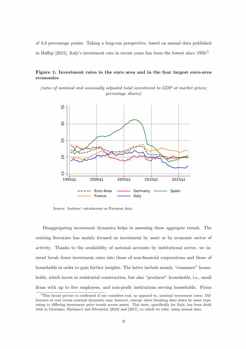


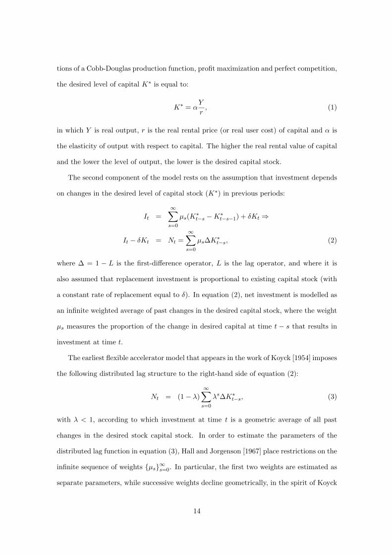


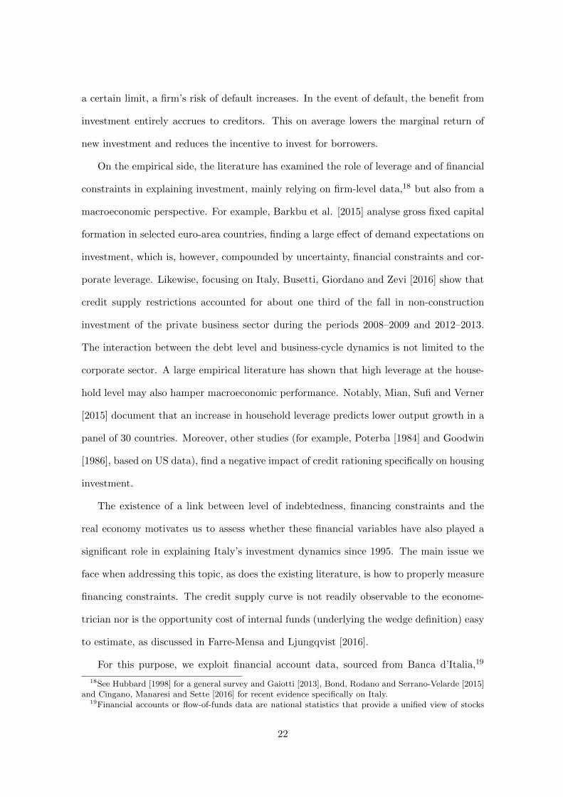

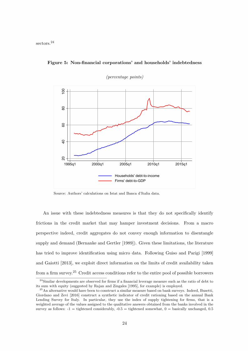

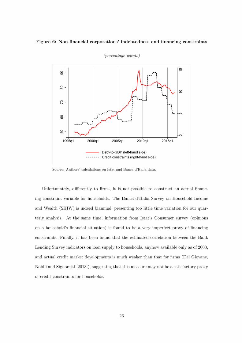


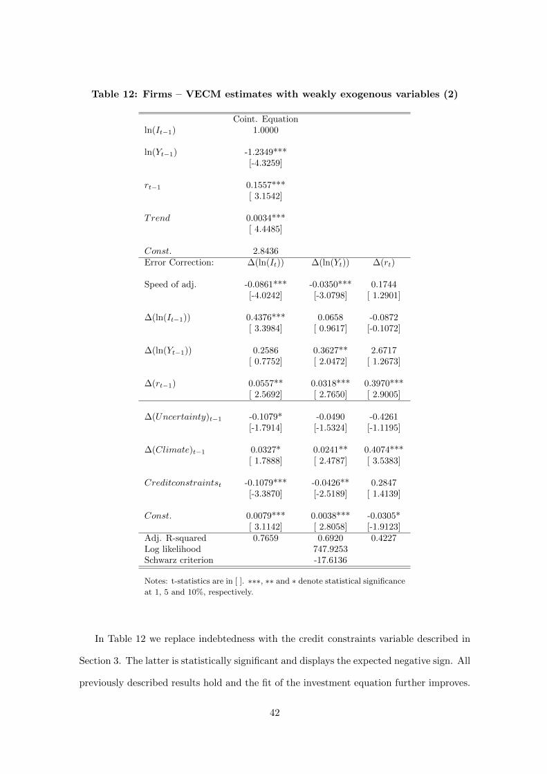


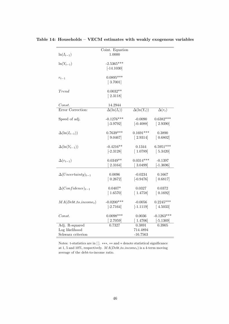


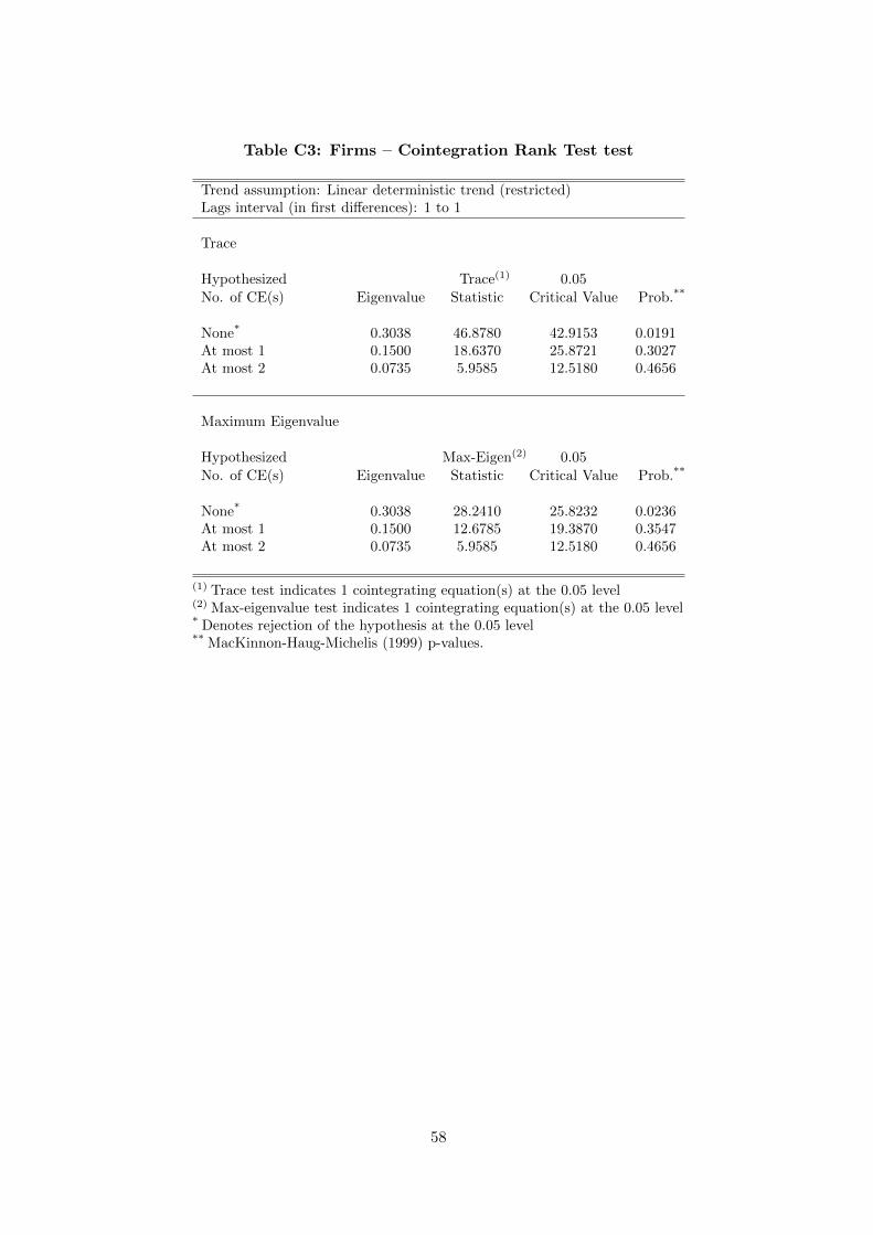


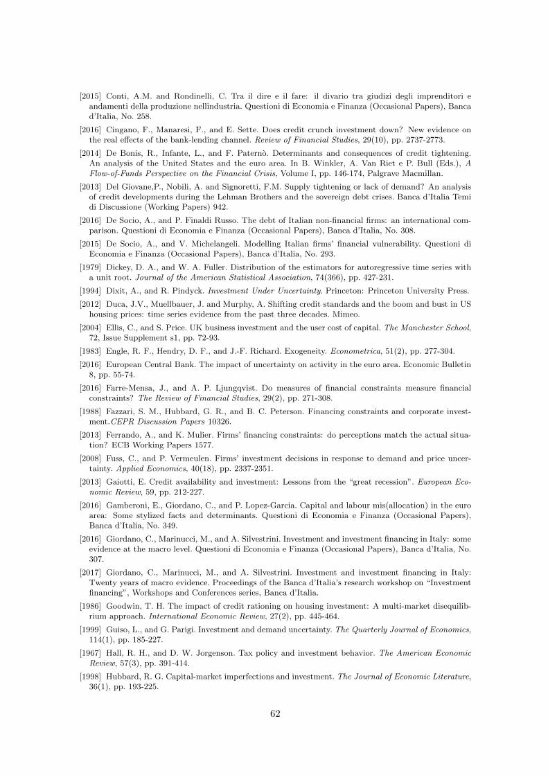


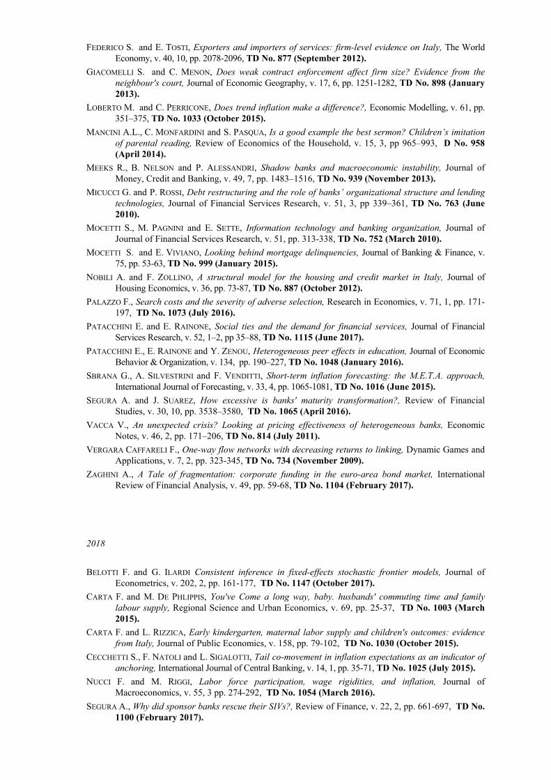


![arxiv.org · arXiv:0803.3486v2 [math.QA] 22 Aug 2008 NEW TECHNIQUES FOR POINTED HOPF ALGEBRAS NICOLAS ANDRUSKIEWITSCH AND FERNANDO FANTINO´ Abstract. We present techniques that allow](https://static.documents.pub/doc/80x56/5f7ee9b5fc4492603729ef17/arxivorg-arxiv08033486v2-mathqa-22-aug-2008-new-techniques-for-pointed-hopf.jpg)


