+ All Categories
Home > Documents > TEMPERATURE DEPENDENT CONTROL By JASON C. FULLER A thesis …

TEMPERATURE DEPENDENT CONTROL By JASON C. FULLER A thesis …

Date post: 09-Dec-2021
Category:
Upload: others
View: 1 times
Download: 0 times
Share this document with a friend
85
TEMPERATURE DEPENDENT CONTROL OF COMMUNITY ENERGY STORAGE DEVICES By JASON C. FULLER A thesis submitted in partial fulfillment of the requirements for the degree of MASTER OF SCIENCE IN ELECTRICAL ENGINEERING WASHINGTON STATE UNIVERSITY School of Electrical Engineering and Computer Science May 2010
Transcript

TEMPERATURE DEPENDENT CONTROL

OF COMMUNITY ENERGY

STORAGE DEVICES

By

JASON C. FULLER

A thesis submitted in partial fulfillment of

the requirements for the degree of

MASTER OF SCIENCE IN ELECTRICAL ENGINEERING

WASHINGTON STATE UNIVERSITY

School of Electrical Engineering and Computer Science

May 2010

ii

To the Faculty of Washington State University:

The members of the Committee appointed to examine the thesis of JASON C.

FULLER find it satisfactory and recommend that it be accepted.

________________________________________

Scott Hudson, Ph.D., Chair

________________________________________

Mohamed A. Osman, Ph.D.

________________________________________

Kevin P. Schneider, Ph.D.

iii

ACKNOWLEDGEMENTS

For his mentorship, constant guidance, and confidence, I’d like to thank Kevin Schneider

for all that he has done to help me succeed. His knowledge and dedication have been an

inspiration to me, and I hope to aspire to his example. And to Scott Hudson, for his dedication to

improving the education of young engineers and his tireless work to provide for each and every

student, I don’t think he’ll ever get enough credit.

I want to thank my parents for having always been there when I needed them, and for all

of their loving support, which has made everything I accomplish possible.

Finally, I’d like to thank my wife, Deb. She had to put up with me during this process, so

that’s saintly enough. However, her love and words of encouragement made all of this possible,

and I don’t think I could ever thank her enough.

iv

TEMPERATURE DEPENDENT CONTROL

OF COMMUNITY ENERGY

STORAGE DEVICES

Abstract

by Jason C. Fuller, M.S.

Washington State University

May 2010

Chair: Scott Hudson

As the electrical infrastructure of the United States ages, and stresses are increased on the

generation and transmission systems due to growing customer loads, the electrical system is

operating at a point far closer to its operational limits. Additional resources will be needed to

meet the demands of customers. While previous system upgrades tended towards increased

generation and transmission assets to meet the customer demand, other options have come to the

forefront in recent years. Distributed Energy Resources (DER) are an alternate means of

increasing the capabilities of the electrical system, using small-scale resources located close to

the load to provide load reduction or a source of generation. While a number of DER

applications exist, this paper will focus on the applicability of Community Energy Storage (CES)

devices. CES devices are small-scale battery systems, designed to operate on the secondary side

v

of the residential transformer, and provide various benefits by storing and the applying power

directly to the load. A variety of applications concentrate on controlling these devices from a

centralized control unit. However, this paper will present a method that allows for localized

control of the CES device to operate in a manner that provides system wide benefits, utilizing the

temperature dependency of residential heating, ventilation, and air conditioning (HVAC) loads.

The control method, designed to operate as a stand-alone application, or in conjunction with

other control modes or with a centralized control unit, will be shown in operation on a single

transformer. Finally, analysis on simple generation, transmission, and market systems will

demonstrate the ability of the CES device to help alleviate stress on the system as whole.

vi

TABLE OF CONTENTS

Chapter 1: Introduction .................................................................................................................................................. 1

Chapter 2: Modeling and Simulation Environment ....................................................................................................... 6

2.1: GridLAB-D ........................................................................................................................................................ 7

2.2: Load Modeling ................................................................................................................................................... 9

Chapter 3: Energy Storage Systems............................................................................................................................. 18

3.1: Batteries ........................................................................................................................................................... 18

3.2: Thermal Energy Storage................................................................................................................................... 19

3.3: Super-Capacitors .............................................................................................................................................. 20

3.4: Superconducting Magnetic Energy Storage ..................................................................................................... 20

3.5: Pumped Hydro Storage .................................................................................................................................... 21

3.6: Flywheels ......................................................................................................................................................... 21

3.7: Compressed Air Storage .................................................................................................................................. 22

3.8: Community Energy Storage ............................................................................................................................. 22

Chapter 4: Control System........................................................................................................................................... 26

4.1: Introduction of Control Mode .......................................................................................................................... 26

4.2: Example of Operation ...................................................................................................................................... 31

Chapter 5: Applications and Results ............................................................................................................................ 42

5.1: Feeder Model and Simulations ......................................................................................................................... 42

5.2: System Wide Benefits of CES ......................................................................................................................... 52

5.2.1 Reduced Emissions .................................................................................................................................... 53

5.2.2 Deferred System Upgrades ........................................................................................................................ 56

vii

5.2.3 Reduced Wholesale Price of Power ........................................................................................................... 58

Chapter 6: Concluding Remarks and Future Work ...................................................................................................... 60

Appendix A ................................................................................................................................................................. 62

A.1: Forward-Back Sweep Method ......................................................................................................................... 62

A.2: Three Phase Current Injection Method ............................................................................................................ 63

Appendix B .................................................................................................................................................................. 65

B.1 Implemented Code ............................................................................................................................................ 65

Bibliography ................................................................................................................................................................ 71

viii

LIST OF FIGURES

Figure 1 : Flow diagram of ETP model [26]................................................................................................................ 11

Figure 2 : Load shape of a single home. ...................................................................................................................... 13

Figure 3 : Load shape of eight homes. ......................................................................................................................... 13

Figure 4 : Load shape of an aggregate of 100 homes. ................................................................................................. 14

Figure 5 : Scheduled load shape .................................................................................................................................. 14

Figure 6 : Load demand as a function of air temperature on 100 simulated homes. ................................................... 16

Figure 7 : CES device next to a standard pad top transformer [53]. ............................................................................ 23

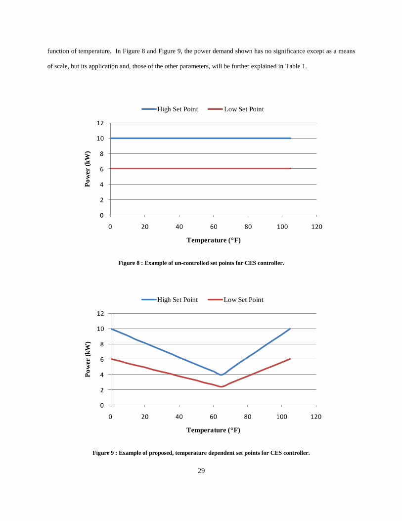
Figure 8 : Example of un-controlled set points for CES controller. ............................................................................ 29

Figure 9 : Example of proposed, temperature dependent set points for CES controller. ............................................. 29

Figure 10 : Power demand on low temperature day. ................................................................................................... 32

Figure 11 : Power demand on high temperature day. .................................................................................................. 32

Figure 12 : Example using set points in Table 2 for controller. ................................................................................... 34

Figure 13 : Power demand on low temperature day while using CES device. ............................................................ 35

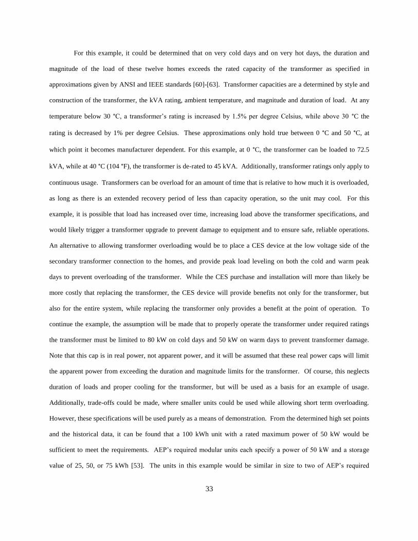
Figure 14 : Depth of discharge of the battery on a cold day. ....................................................................................... 36

Figure 15 : Power demand on high temperature day while using CES device. ........................................................... 36

Figure 16 : Depth of discharge of the battery on a warm day. ..................................................................................... 37

Figure 17 : Average temperature day load demand. .................................................................................................... 38

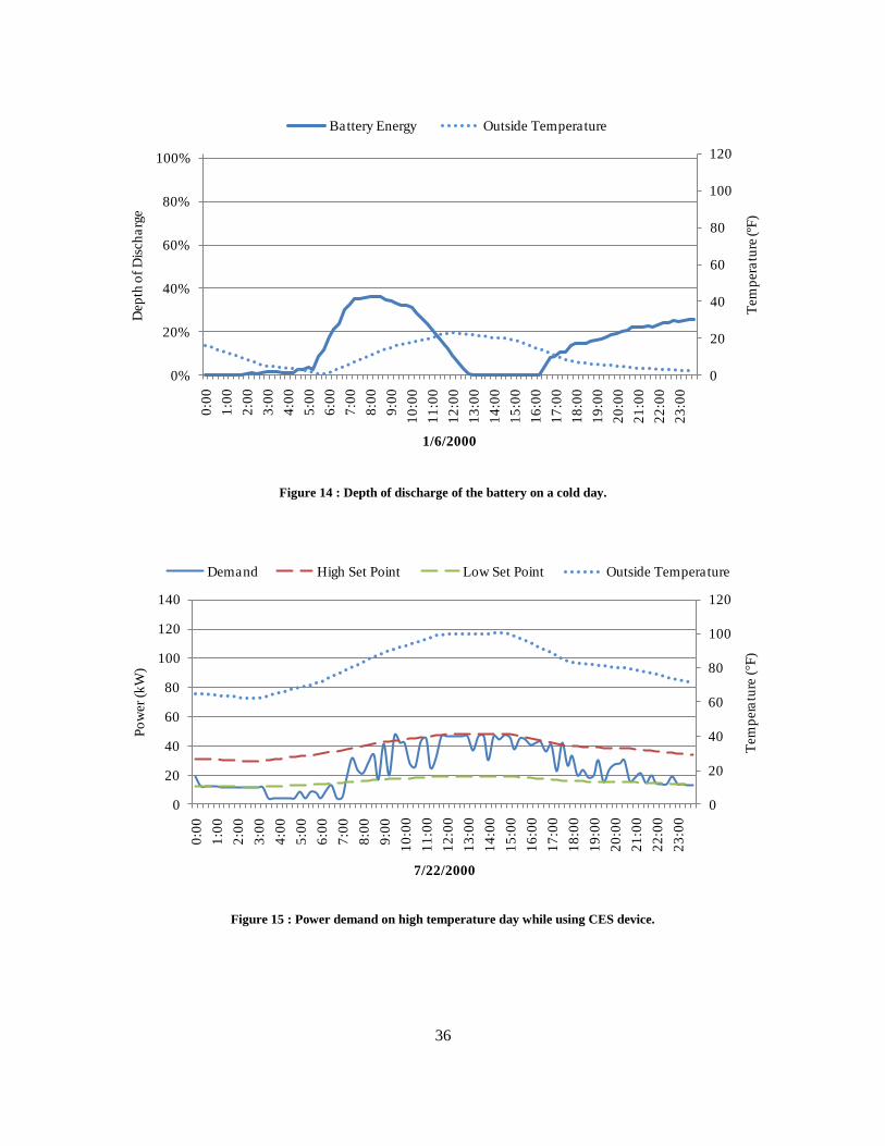
Figure 18 : Average temperature day load demand with battery control. .................................................................... 39

Figure 19 : Depth of discharge of the battery on an average temperature day. ........................................................... 39

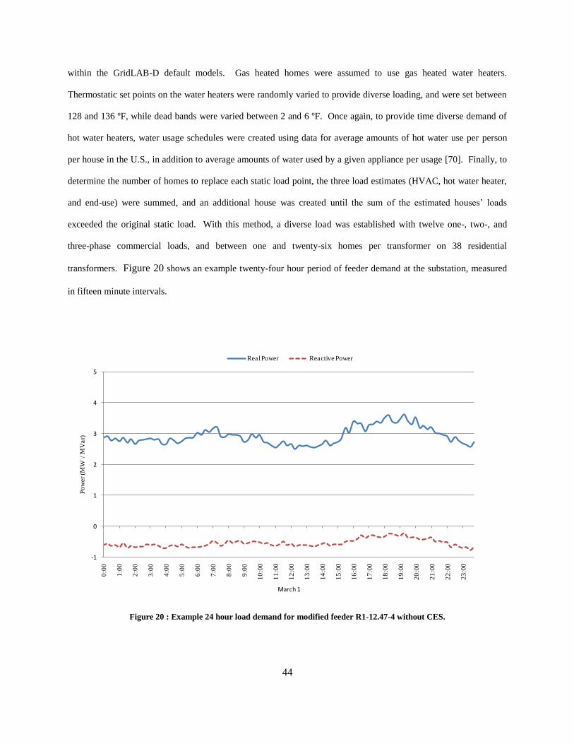
Figure 20 : Example 24 hour load demand for modified feeder R1-12.47-4 without CES. ........................................ 44

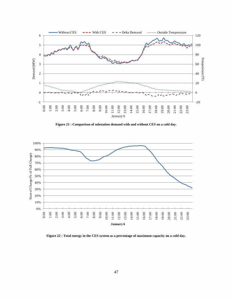
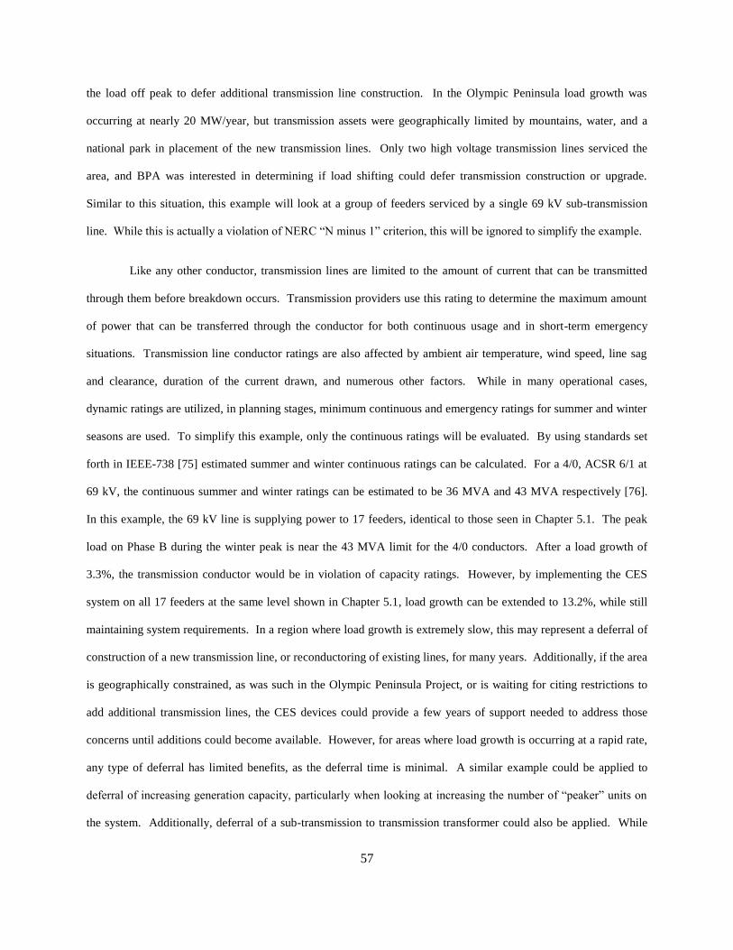
Figure 21 : Comparison of substation demand with and without CES on a cold day. ................................................. 47

Figure 22 : Total energy in the CES system as a percentage of maximum capacity on a cold day. ............................ 47

Figure 23 : Comparison of substation demand with and without CES on a mild temperature day. ............................ 48

Figure 24 : Total energy in the CES system as a percentage of maximum capacity on a mild temperature day. ........ 48

Figure 25 : Comparison of substation demand with and without CES on a warm day. ............................................... 49

Figure 26 : Total energy in the CES system as a percentage of maximum capacity on a warm day. .......................... 49

ix

Figure 27 : Load duration curves for base case and CES case (sensitivity = 1.6). ...................................................... 51

Figure 28 : Difference between load duration curves for base case and CES case. ..................................................... 51

Figure 29 : Dispatch of generation for base case of Chapter 5.1 using Washington St. generational mix. ................. 54

Figure 30 : Dispatch of generation for base case of Chapter 5.1 using U.S. generational mix. ................................... 54

x

LIST OF TABLES

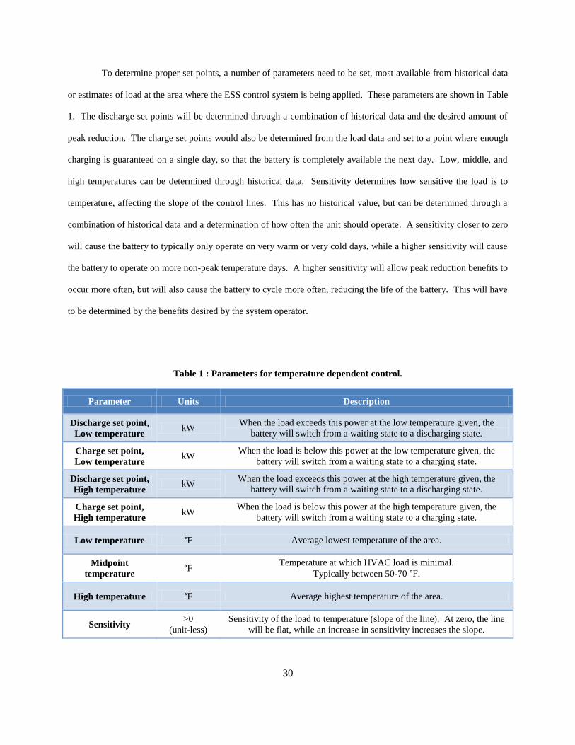
Table 1 : Parameters for temperature dependent control. ............................................................................................ 30

Table 2 : Example set points for controller. ................................................................................................................. 34

Table 3 : Temperature sensitivity and its effect on selected values. ............................................................................ 40

Table 4 : Residential transformers and the number of models used at each location. ................................................. 46

Table 5 : Generation fuel mixes for Washington State versus U.S. ............................................................................. 53

Table 6 : Average emissions for each fossil fuel type (lbs/MWh). .............................................................................. 55

Table 7 : Change in emissions from base to CES case using Washington St. and U.S. generation mixes. ................. 55

1

CHAPTER 1: INTRODUCTION

In 1896, hydroelectric power was generated at Niagara Falls and electricity was delivered twenty miles to

supply industrial areas in Buffalo, New York. This was a turning point in the history of electricity, eventually

leading to a sprawling system of interconnected generation, transmission, and distribution systems throughout the

United States. This moved away from Thomas Edison’s plans for supplying generation local to the load. From this

sprawling system, the North American electrical power delivery system has grown ever more complicated and has

been called “the world’s largest and most complex machine” [1]. As complexity increases, while the century old

system ages, concerns are growing over the future of the U.S. electrical infrastructure [2]. The U.S., as a nation, is

the largest consumer and producer of electrical power in the world, sustaining its economy on efficient and

affordable delivery of power [3]. Consumer load has increased substantially, while the corresponding creation of

new electrical generation has not kept pace, increasing pressure on the transmission system while costs of building

have also increased [4]. Since 1982, customer demand has increased at a rate 25% greater than that of the

transmission system that supports it [5], and while generation capacity has not fallen off as rapidly, generation

growth is far exceeded by load growth. Reasons vary, including increased cost of construction, limited site options,

rising fuel costs, carbon and chemical emission concerns, environmental contamination and destruction, and

regulatory related issues. As a result, the electrical infrastructure of the United States is now operating at a point

which is much closer to its operating capacity, raising concerns about the unprecedented level of risk and

uncertainty of the electrical industry [2]. Historically, as customer load increased over time, capital assets, including

generation and transmission, were built to meet the needs of the system, including customer load, system losses, and

operational safety margins.. This approach is a viable option, as long as there is a continued expansion of both

transmission and generation assets to track the increased consumer demand. However, there is increasing resistance

to the creation of power plants, especially with coal or nuclear based plants, and concern over the long term effects

of power generation on the environment. Additionally, “not in my backyard” (NIMBY) attitudes toward

construction of generating plants and right-of-ways for new transmission, sub-transmission, and distribution lines

create difficulties for planners when trying to improve the electrical infrastructure through building of large-scale

transmission and generation assets. While new sources of electrical generation, such as wind and solar, have a

2

number of proponents and have distinct advantages to classical, fossil fuel generation, each has their own integration

problems that must be dealt with before large scale penetration into the generation market can occur. While in the

short term, customer load has decreased due to the downturn of the economy, long term projections show a distinct

increase in customer demand. Combined with difficulties in increasing the necessary transmission and generation

assets to meet this demand, concerns are growing over the future of the U.S. electrical system and its ability to meet

the future needs of the country.

An alternate to the historically large capital projects is the use of distributed generation (DG) and

distributed energy resources (DER), providing a means for load shifting and storage of energy which can be applied

to transmission and distribution assets [4]. A large number of utilities across the U.S. are looking at DG and DER as

possible cost-effective alternates to building additional centralized generation plants and transmission level assets

[6]-[9]. DG relocates power generation, foregoing the concept of large, centralized plants using high voltage

transmission lines as a means to move the power, to a more decentralized concept, where power is generated close to

the load it is supplying. While the DG does not have the economies of scale that make central generation attractive,

there are a number of other significant advantages [10]. Initial investment costs are typically lower, since DGs are

typically much smaller and allow for small incremental increases of power generation, 1-10 MW, while centralized

plants generally are on the 100-1000MW scale. Because DG units are located closer to the end users, there is a

decreased demand on transmission assets, resistive losses are reduced, equipment degradation due to thermal

stresses can be reduced, and the need for reactive compensation can be somewhat mitigated. Of major benefit is the

deferral of equipment upgrades on both the distribution and transmission system, combined with congestion relief

on heavily loaded systems. DG units provide system level relief by generating power near the load, but additional

benefits can be realized by using technologies that control the end-use load or store energy near the load. By

providing multiple levels of benefits, the high cost of DG and DER devices can be further offset. There is some

disagreement in the literature as to what constitutes a DER resource, some stating that DG and DER are

synonymous, while others recognize that other resources can be used as a distributed energy resources. For the

purpose of this discussion, DG will be considered a subset of DER, and includes other distributed energy

technologies beyond generation, including energy storage, co-generation heat plants, demand response systems,

hydrogen stations, or any other energy technology that can be deployed local to its usage. Gumerman et. al.

3

provides a summary of 17 societal and economic advantages and disadvantages that can be associated with DER

integration, and ranks them relative to their benefits [11], while Iannucci et. al provides a detailed breakdown of

potential benefits of DER by reviewing 124 reports across the available literature and selecting the “Top 30” DER

reports [12].

The use of distributed generation plants is not a new idea. In 1882, Thomas Edison created the Pearl Street

Station to service 85 customers and their 400 incandescent light bulbs. Eventually, service was increased to include

508 customers, and transmitted direct current (DC) power at 110 volts and 220 volts over a one-square mile area,

before the station burned down in 1890. However, the geographical area of use was limited by the distance the

power could be transmitted before losses caused the voltage to drop below a usable level. Additionally, for each

voltage level required by customers, an entirely new system had to be created as there was no way to interconnect

different voltage levels. High voltage arc lighting, which used up to 10 kV DC and was being used for city lighting

in New York, and street cars, using 500 V DC, could not be merged with the 110/220 volt system used by residential

customers, requiring multiple systems in a single area. Additionally, most industrial users required a completely

different voltage level, dependent upon their application. The modern electrical system, which uses high voltage

transmission lines, centralized generation plants, and alternating current (AC), can trace its beginnings to the

invention of induction transformers and polyphase generators and motors in the 1880s. George Westinghouse

commercialized Nikola Tesla’s polyphase system, which provided the means to create an inexpensive voltage step-

up and step-down transformer system that allowed power to be generated away from the load it supplied, transmit

the power over long distances at high voltages, and then reduce the voltage back to the varying levels required by

the different customers. At the time, there was no DC equivalent to step-up and step-down transformers, and AC

power eventually became the standard in the U.S. This was eventually demonstrated at Niagara Falls, and the North

American system slowly evolved to Tesla’s proposed framework, moving away from DG applications. Inexpensive

High Voltage DC (HVDC) alternatives do exist today and have been in use for a number of years in transmission

systems [13], and as the technology matures and prices drop, low voltage DC applications are increasing in

application.

4

As the modern electrical infrastructure of the U.S. evolved, from a single AC transmission line connecting

Niagara Falls and Buffalo, NY to a complex interweave of transmission lines stretching the length of the U.S.,

generation and load have become further separated. This has led to a system where load is generally able to behave

without major restriction, while generation must be dispatched to meet the demands of the loads and also the losses

within the transmission system. In other words, when a customer turns on their light switch, the light comes on and

power is delivered, regardless of the demand on the system. One of the visions of the Department of Energy (DOE)

and its application of “Smart Grid” technologies is to engage the load as a resource that is also able to react to a

supply and demand style system, as opposed to current system where generation always tries to meet the current,

unrestricted demand [5]. This top-to-bottom approach for controlling the entire electrical system as a whole has a

huge potential for decreasing expensive peak load instances, and can be greatly assisted by DG and DER devices

[5]. During times of peak loads, such as those found on extremely warm or extremely cold days, utilities and

operators are forced to bring online “peaker” units which only operate during extreme increases in load to track the

peak demand. Peaker units are typically older, expensive to operate, and far less efficient than larger base plants.

This is compounded with the fact that most peaker units sit idle throughout the year, generating no income, but still

must be maintained. DER devices can assist the system by either applying generation directly to the load or

reducing the load so that generation no longer needs to track the demand during these peak events, reducing the need

for peaker units. Peak load management from DER devices, can all serve as a means to defer investment in

generation, transmission, and distribution systems [14].

Naturally, there are a number of disadvantages to using DG and DER devices. Centrally controlled

resources, such as classical generation assets, allow system operators to have direct control over critical attributes of

the system, such as voltage magnitude and reactive power injection, power factor correction, and frequency

regulation. DERs, however, are often not directly controlled by the system operator, and individually are too small

to provide the necessary services needed to have an effect on these parameters. However, when a number of units

are aggregated across a system, their combined size can have an effect on the system. Proper operation of an

individual DER device is relatively unimportant on the system as a whole, but the aggregate effect of those devices

dictates that all of the devices must operate in a coordinated manner to the benefit of the entire system. The “Smart

Grid” concept, as stated by DOE, looks at integrating all of these devices into a two-way communication system,

5

incorporating real-time information and decision making [5]. However, developing and operating this system and

the DERs involved, represents an additional investment to utility companies. This includes not only the resources

themselves, but additional costs, including communication systems needed to move commands and information

back and forth between controllers and the DER, additional protective equipment, or a number of other possible

infrastructure upgrades. While compared to the expense of building a coal or nuclear plant and the requisite

transmission upgrades, this expense may be small, but it still must be addressed as utilities are convinced to adopt

DER technologies. A number of planning issues also occur for the system operator, and can result in adverse effects

upon operation of either the transmission or distribution system. Common problems can include reverse power

flow, islanded systems with active generation, shortened equipment life, and decisions on how to operate a wholly

new system. Although standard practices for addressing some of these issues are set forth in IEEE 1547 [15], in

some cases, unintended consequences can occur [10]. For example, high levels of unconstrained DG penetration

have been shown to increase losses within certain components in distribution systems [16]. When considering

renewable DG resources, such as wind and solar, DG becomes an energy source that cannot be dispatched to meet

load demand, due to the intermittent and unpredictable nature of the fuel source. Energy storage systems (ESSs), in

combination with renewable resources, are fast becoming a popular conceptual alternative to centralized generation,

and should act as a means to mitigate the effects of un-dispatched generation.

Despite the disadvantages, the installation of DER solutions is actively occurring within the United States

and will more than likely continue at an accelerated rate. As of 2005, nearly 12 million DG units were installed

throughout the U.S. with nearly 200 GW of capacity, although mainly for back-up generation purposes at hospitals

and other vital facilities [10] which cannot be used for utility support. Demand response demonstrations have

occurred in a number of utilities throughout the U.S. As discussed, DER integration provides a very unique set of

opportunities and obstacles for planners and operators, and it is up to utility companies to plan for and apply these

technologies, while still providing the same level of service and abiding by current regulations set forth for standards

of service. A number of progressive utilities have begun using DERs in a limited manner, mainly in conjunction

with DOE support of possible implementations of “Smart Grid” technologies.

6

Despite the recent successes of these DER demonstrations, much work needs to be done to enable large

scale deployments, increase its applicability, and provide a distinct advantage over increased centralized generation.

Decreasing costs, while increasing the range of benefits, increasing reliability, increasing the planning data available

to utilities, improving models and operational control mechanisms, are all of utmost concern for integration of DER

systems [10]. This body of work will propose an improvement of a single DER technology, Community Energy

Storage (CES). The following chapters will describe the steps needed to develop a control mode and model for a

CES device, which operates in a manner independent of a centralized control unit. Chapter 2 will describe the

modeling efforts used to accurately represent a distribution system, with particular focus on load modeling. Chapter

3 will provide a brief background of current ESS and CES applications. A description of the proposed control of the

CES device will be provided in Chapter 4, followed by an example of the control system in operation. Simulation

results using the newly proposed method will then be discussed in Chapter 5, where societal and environmental

advantages and disadvantages of the proposed system will be compared. Finally, Chapter 6 will discuss future work

and improvements on the proposed system.

7

CHAPTER 2: MODELING AND SIMULATION ENVIRONMENT

When modeling systems of components, individual and system models of reasonable accuracy are

paramount when considering incremental changes to large, complex systems. Distribution systems, combined with

transmission systems, are highly complex, with numerous interactions between hundreds or thousands of

components, each with their own distinct parameters, behaviors, and controls. A sufficient level of detail in

modeling becomes even more important when looking at the effects of integrating DER onto a distribution or

transmission system, where small, cumulative changes are aggregated to provide large scale effects. One advantage

of using a simulation environment like GridLAB-D is its ability to assist in understanding the effects of small scale

changes to highly complex systems, with all of the interactions that occur between individual models. As GridLAB-

D allows for the analysis of multi-disciplinary problems, incorporating a steady-state, time-series solver, it is ideal

for looking at the effects of energy devices on a system, as opposed to solving single power flow operations. As

there is no requirement for the use of reduced-order models, the danger of erroneous assumptions can be averted

[17]. As all simulations in this body of work use GridLAB-D, some of the capabilities and benefits of using

GridLAB-D, will be described in the following sections.

2.1: GRIDLAB-D

GridLAB-D is the first of a new generation of distribution system simulation technologies [17]. It is a

flexible, open-source simulation environment, designed by Pacific Northwest National Laboratories (PNNL) in

collaboration with industry and academia, for the Department of Energy’s (DOE) Office of Electricity Delivery and

Energy Reliability (OE) [18]. GridLAB-D was designed and created as a test-bed for research and analysis of

“smart grid” technologies and their effects upon distribution and transmission systems, and is continually in

development. A few of the main areas of focus include detailed modeling of three-phase, unbalanced distribution

systems, highly detailed load modeling, and control mechanisms for DERs. GridLAB-D is a simulation

environment, using time-variant models and tying together multiple areas of discipline to create a more complex

interweave of modeling. It is capable of studying distribution utility system behaviors, ranging from a few seconds

8

to decades, while simulating the interactions between physical phenomenon, business systems, markets, regional

economics, consumer behavior, and a whole host of other possibilities [17]. Each device within the GridLAB-D

simulation environment is modeled independently, as described by a range of differential and difference equations,

each solved locally in both state and time. The interactions of the individual models are incorporated by the core of

the simulator, and then the individual models are re-solved with new information provided by the interactions. This

proceeds in an iterative fashion until a solution is reached. Traditional power flow analysis can be enhanced through

a series of quasi-steady state time-series solutions, detailed end-use load models, thermal and chemical energy

models, and generator models, all incorporated into the GridLAB-D simulation environment. More information can

be found on the official website [19]. A brief background into the importance of these features, how they apply to

this work, and how they are implemented into GridLAB-D will follow.

Unbalanced three-phase distribution systems are the standard within the United States, but have often been

modeled in a similar fashion to transmission systems, with per-phase or symmetric component equivalent models.

However, within distribution systems, unbalanced loading across phases, areas with less than all three-phases, and

circular currents are quite common, and cannot be accounted for accurately within balanced three phase models. In

the past, symmetrical component and balanced phase models have been used by industry standard software [20]-

[22] to approximate the condition of distribution systems. For a majority of utility planning and operation studies,

these approximations have been sufficient. However, when considering the effects of DER integration, it becomes

much more important to accurately model the effects of an unbalanced system and how it interacts with the various

distributed technologies. DG, energy storage, and demand response devices are typically attached only to a single-

phase on a distribution system, but through the inductive and capacitive coupling of the parallel lines, can also affect

other phases. This makes balanced solutions impractical for studies using DER. Additionally, DER units provide

system wide benefits by aggregating small, individual benefits. If these incremental benefits are not accurately

modeled, or are lost due to inaccuracies of the distribution model, then the aggregated benefits of the technology

cannot be realized. By more accurately modeling the unbalanced three-phase system, the DER device, the end-user

load, and all of the complex interactions that exist between them, a more accurate representation of the affects can

be analyzed. GridLAB-D has the ability to more accurately model each of these in a modular, agent-based system,

where objects designed by users or developers can incorporate nearly any level of necessary detail and a core

9

module handles the interactions between each object. The “powerflow” module is used to model distribution

systems, and uses two distinct algorithms to handle three-phase unbalanced power flow solution methods, selectable

by the user. The first is the Forward-Backward Sweep (FBS) method presented by Kersting [23], while the second

is the Three-Phase Current Injection Method (TCIM) presented by Garcia et al. [24]. Further description of the

methods used can be found in Appendix A.

2.2: LOAD MODELING

While a significant amount of work has been done to accurately model the physical models of the electrical

systems [25][26], end-use loads have not received the same level of attention, especially within distribution systems.

Distribution system loads are typically described by a time-invariant combination of constant power, constant

current, and constant impedance elements (ZIP), either in a Delta or Wye connection [23]. A common practice used

within commercial software packages is a scheduled time-variant model that varies the ratio of the ZIP components,

along with a load growth schedule, typically with one hour time intervals [20]-[22]. While these classical load

models are available for use in GridLAB-D, more complex models can also be used or created. A large majority of

distribution loads have not only time-dependent ZIP components, but are also described as a function of

temperature, humidity, human interaction, and a number of other independent variables that cannot be accurately

described by ZIP schedules. These loads can typically be classified as thermal loads and encompass such loads as

heating, ventilation, and air conditioning units (HVACs), hot water heaters, clothes washers and driers, and

refrigerators to name a few. In non-gas supplied homes, HVAC units and hot water heaters typically represent the

largest single energy loads in a home, consuming on average over 7700 kWh per year per home [27], but cannot be

well described by a scheduled load shape. GridLAB-D uses an equivalent thermal parameter (ETP) model to

accurately represent the residential load of the HVAC unit [26], which has been shown to accurately represent the

heat flow and HVAC response of residential and commercial buildings [28]-[31]. The ETP model has three sources

of heat input; solar radiation, internal gains from human and appliance waste heat, and the HVAC system. The

temperature of the mass of furniture and walls and the mass of air within the house are then coupled through the

flow chart provided in Figure 1 and the second-order differential equation described by

10

𝐶𝑚𝑎𝑠𝑠 𝐶𝑎𝑖𝑟

𝑈𝐴𝑚𝑎𝑠𝑠

𝑑2𝑇𝑎𝑖𝑟

𝑑𝑡2+

𝐶𝑚𝑎𝑠𝑠 (𝑈𝐴𝑒𝑛𝑣 + 𝑈𝐴𝑚𝑎𝑠𝑠 )

𝑈𝐴𝑚𝑎𝑠𝑠

𝑑𝑇𝑎𝑖𝑟

𝑑𝑡+ 𝑈𝐴𝑒𝑛𝑣 𝑇𝑎𝑖𝑟 = 𝑄𝑚𝑎𝑠𝑠 + 𝑄𝑎𝑖𝑟 + 𝑈𝐴𝑒𝑛𝑣 𝑇𝑜𝑢𝑡 ( 2.1)

where:

𝐶𝑎𝑖𝑟 is the air heat capacity

𝐶𝑚𝑎𝑠𝑠 is the mass heat capacity

𝑈𝐴𝑒𝑛𝑣 is the gain/heat loss coefficient between the air and outside

𝑈𝐴𝑚𝑎𝑠𝑠 is the gain/heat loss coefficient between the air and mass

𝑇𝑜𝑢𝑡 is the outside air temperature

𝑇𝑎𝑖𝑟 is the air temperature inside the house

𝑇𝑚𝑎𝑠𝑠 is the temperature of the mass inside the house

𝑇𝑠𝑒𝑡 is the temperature control set point of the HVAC system

𝑄𝑎𝑖𝑟 is the heat rate to the air inside the house

𝑄𝑔𝑎𝑖𝑛𝑠 is the heat rate from the appliance waste heat

𝑄ℎ𝑣𝑎𝑐 is the heat rate from the HVAC system

𝑄𝑚𝑎𝑠𝑠 is the heat rate to the mass inside the house

𝑄𝑠𝑜𝑙𝑎𝑟 is the heat rate from solar radiation gains

11

Figure 1 : Flow diagram of ETP model [26].

Using the ETP model, with proper variable definitions that may vary over time, an accurate electrical load can be

determined from a residential end-use. The difference between loads with thermal cycles and those without are

further described in [26]. In addition to the thermal model of the HVAC system, GridLAB-D also incorporates a

two-node thermal state model of the hot water heater in addition to classical ZIP models. All of these loads will be

used in this paper as a means to more appropriately model the end-use residential loads and their interactions with

the electrical distribution systems.

As an example, Figure 2 through Figure 5 show the differences between a full thermodynamic model of a

single home, a combination of eight homes each using different input variables, the aggregation of one hundred

individually designated homes, and a commonly used schedule driven load shape, each over a 24 hour period. The

loads represented within these homes include HVAC systems, hot water heaters, and a ZIP light and plug load

12

recorded at one minute time intervals. Figure 5 represents the commonly seen load pattern that is typical at the

substation level. By applying this load shape at all of the load locations, with proper scaling factors, the load at the

substation will appear nearly identical. This is often the approach of commercial software packages, typically with

even less resolution. While this accurately portrays the aggregation of all the loads on the system, it does not

accurately represent what the individual loads are doing at each individual point along the system, nor does it

accurately represent the response of individual objects within the system. Figure 2 represents the load demand of a

single home, and shows that at a close level of inspection, a residential end-use does not behave like a smoothed

load shape, but rather with peaking pulse trains in addition to more traditional constant loads. The different loads

can be seen turning on and off at various times throughout the day, dependent upon non-electrical conditions,

including temperature, humidity, and human interaction. While Figure 2 looks very dissimilar to the commonly

seen load shape in Figure 5, as progressively more homes are added to the system, these two load shapes will

converge. This can be seen in the progression of Figure 3 and Figure 4. Figure 3 shows eight individual residential

homes, while Figure 4 shows the aggregation of one hundred residential homes, each with their own thermal

parameters and set points, leading to differing duty-cycles. Figure 4 now has a load shape similar to the

characteristic load shape pattern of Figure 5, but more accurately represents how each individual load is behaving

independently. This is an example of load diversity and is important in determining the placement and control of

DER devices and how they respond to the loads around them. These effects also become important when looking at

DERs that use thermal mass as a means of shifting the load. This type of DER uses control signals of various types

to adjust thermostatic set points, which allows the thermal inertia of the building to keep the air temperature

relatively mild for short periods of time. While this may play an important part in correctly modeling the effects of

DER on a distribution system, it will not play a significant role in the simulations to follow.

13

Figure 2 : Load shape of a single home.

Figure 3 : Load shape of eight homes.

0

2

4

6

8

10

12

0:0

0

1:0

0

2:0

0

3:0

0

4:0

0

5:0

0

6:0

0

7:0

0

8:0

0

9:0

0

10

:00

11

:00

12

:00

13

:00

14

:00

15

:00

16

:00

17

:00

18

:00

19

:00

20

:00

21

:00

22

:00

23

:00

Po

wer

(kW

)

0

5

10

15

20

25

30

35

40

45

50

0:0

0

1:0

0

2:0

0

3:0

0

4:0

0

5:0

0

6:0

0

7:0

0

8:0

0

9:0

0

10

:00

11

:00

12

:00

13

:00

14

:00

15

:00

16

:00

17

:00

18

:00

19

:00

20

:00

21

:00

22

:00

23

:00

Po

wer

(kW

)

14

Figure 4 : Load shape of an aggregate of 100 homes.

Figure 5 : Scheduled load shape

Another consideration when dealing with residential and commercial loads that is often neglected is the

impact of weather on the shape, demand, and duration of load. It has been repeatedly shown that there is a

correlation between temperature, humidity, and other meteorological phenomena and load duration and demand,

where temperature appears to have the strongest correlation [32]-[34]. Most studies have focused on warm air

0

50

100

150

200

250

300

350

400

450

0:0

0

1:0

0

2:0

0

3:0

0

4:0

0

5:0

0

6:0

0

7:0

0

8:0

0

9:0

0

10

:00

11

:00

12

:00

13

:00

14

:00

15

:00

16

:00

17

:00

18

:00

19

:00

20

:00

21

:00

22

:00

23

:00

Po

wer

(kW

)

0

50

100

150

200

250

300

350

400

450

0:0

0

1:0

0

2:0

0

3:0

0

4:0

0

5:0

0

6:0

0

7:0

0

8:0

0

9:0

0

10

:00

11

:00

12

:00

13

:00

14

:00

15

:00

16

:00

17

:00

18

:00

19

:00

20

:00

21

:00

22

:00

23

:00

Po

wer

(kW

)

15

temperatures and humidity, and the effect it has upon the air conditioning load; however, similar, but not identical,

effects can be extrapolated to cold weather situations as well as warm. GridLAB-D models three different types of

HVAC heating fuel sources; gas, which includes any type of fuel burning system, resistance, which represents any

type of electrical resistive heating system (baseboard heating, space heaters, etc.), and heat pumps, which represent

any two-way heat transfer system which is a paired heating and cooling system. Gas and other non-electrical forms

of heating are still the most common throughout the U.S.; however, exact composition is highly dependent on the

region of the U.S. and age of the industrial, commercial, or residential buildings [35]. Figure 6 represents a

simulation of one hundred single-family homes in GridLAB-D and the load demand of the HVAC as a function of

temperature over the course of an hour. It can be seen that homes using resistive heating are near linear as a

function of outside air temperature, heat pump homes are non-linear, and the blended average with all three types of

heating are near linear. For the case shown in Figure 6, all other factors, including weather factors such as humidity

and solar radiation, and human factors such as heating and cooling thermostat set points and internal gains from

waste heat, are removed to isolate the effects of outside air temperature on the load of the HVAC. Figure 6 indicates

that the heating portion of the HVAC load of an aggregate of homes can be roughly approximated with a linear

function, where the relative mixture of heating types is an indicator of the slope of the line. While this is not a

perfect fit, the rough approximation can still be used in the control method to be shown later. This will only not be

the case, when the mixture of heating types has a high penetration of heat pumps, which is typically only common in

areas with mild heating and cooling needs and newer construction [35].

16

Figure 6 : Load demand as a function of air temperature on 100 simulated homes.

In Figure 6, when looking at demand for temperatures warmer than the midpoint temperature of

approximately 70 °F, air conditioning or cooling, as opposed to heating, is now the primary load. The temperature

and demand of the midpoint is dependent on the end-users, as both will depend on the combination of

thermodynamic properties of the load in question. Heating and cooling set points, as set by the consumers on their

thermostats, insulation properties of the homes, and efficiencies of the HVAC units will all play a part in

determining the midpoint temperature and demand. As heating and cooling consumption is the largest single portion

of household demand, representing over 25% of total residential energy usage in the U.S. [27], while typically

contributing a much larger portion of the peak load demand, it is important to understand the characteristics of the

HVAC system and their dependencies on external conditions. Utility planners use temperature and other

meteorological predictions as indicators for short-term load forecasting, in addition to historical data [33][34]. It can

be seen from the GridLAB-D results in Figure 6, that the aggregate cooling load for residential homes are roughly

linear as a function of temperature. The linear to slightly quadratic relationship of residential home HVAC load to

0

200

400

600

800

1000

1200

1400

0 20 40 60 80 100 120

HV

AC

dem

an

d (k

Wh

)

Outdoor Temperature ( F)

Heat Pump Resistive Heat Gas Heat Blended

Heating Air Conditioning

17

temperature has been shown numerous times through empirical studies, although typically only over short changes

in temperature [32][34]. For the purpose of the following discussions, it will be assumed that the HVAC load mixes

are near linear in nature. This assumption will be used to predict the load as a function of temperature, which shall

then be used to control the behavior of the energy storage device. This will be explained in more detail in Chapter 4.

18

CHAPTER 3: ENERGY STORAGE SYSTEMS

Energy Storage Systems (ESSs) encompass a large range of technologies; including chemical batteries such

as Sodium-Sulfur (NaS), Nickel-Cadmium (Ni-Cd), Lead-acid, and Lithium-ion (Li-Ion), flow batteries such as

Zinc-Bromide (ZnBr) and vanadium redox (VO), thermal storage devices, electrochemical super-capacitors,

Superconducting Magnetic Energy Storage (SMES), pumped hydro, flywheels, and Compressed Air Energy Storage

(CAES). The built and proposed installations are wide and varied, highly dependent upon the type of technology.

Some are ideal for use at the transmission level, while some are more ideal for small scale applications. A brief

description of the main ESS technologies, the state of the technology development, and its ability to be implemented

at the utility level will be presented.

3.1: BATTERIES

Two main types of batteries exist in utility applications; chemical and flow. Chemical batteries operate by

physically separating two electrodes in an electrolytic solution. When electricity is required, a chemical reaction

releases ions from one electrode (anode) into the solution and deposits oxides on the other (cathode). Reversing the

operation charges the battery. Battery systems have the advantage that they are modular and quiet, non-polluting,

and can typically be installed in a short period of time, which is especially advantageous when located in city

neighborhoods [36]. The main drawback of chemical batteries is the battery life cycle, which is effected by the

depth of discharge and temperature regulation. In most applications, this may mean additional controls are needed

to control the number and depth of discharges, and additional temperature regulation devices such as heaters or fans

are often included. NaS and Li-Ion batteries have gained much recent attention as a rapidly developing technology,

with a number of test facilities in operation within the U.S. and Japan. NaS batteries have been used in recent utility

applications, while Li-Ion batteries have been used in electronics for years. However, with Li-Ion now being used in

a number of Plug-In Hybrid Electrical Vehicle (PHEV) applications, it is gaining attention with utilities for use on

distribution systems and as a CES device. Lead-acid and Ni-Cd are both mature technologies, but low cycle life for

lead-acid and concerns about Cadmium availability and its effects on the environment have made these technologies

19

less desirable for utility applications [37]. Flow battery technologies, also known as regenerative fuel cells, store

and release energy through a series of electrochemical reactions across a membrane separating two electrolytic

solutions, and are only limited in size by the amount of fluid available. Flow batteries have a lower energy density

than equivalent chemical batteries, and typically require a larger footprint for operation [38]. The large footprint

will more than likely prevent the use of flow batteries in CES devices, but the mobility of the system in conjunction

with easy scalability, has utilities showing interest in use as a mobile, substation level storage device.

Battery systems are most appropriate in distribution and transmission systems for storing small to medium

amounts of energy. They have been shown, in conjunction with back to back power supplies, to effectively provide

voltage regulation, frequency control, interrupt support, VAR support, and spinning reserve for short-term peak load

reduction [36]. A number of DOE sponsored battery storage systems have already been implemented throughout the

United States, as tests into the applicability of the technologies. American Electric Power (AEP) has installed a 100

kW, 720 kWh, single commercial building NaS demonstration in 2002 [7], a 1.2-MW, 7.2MWh NaS system in

Charleston, West Virginia in 2006 [6][39], and three 2-MW, 14.4 MWh NaS systems across three feeders in 2008,

among others [40]. Chino, California, Puerto Rico, and Utah, among others, are also operating multi-MW battery

storage systems [41]. Southern California Edison and the Electric Power Research Institute (EPRI) demonstrated

the effectiveness and drawbacks of lead-acid batteries for a number of services, including voltage, VAR, and

frequency control and load leveling [4]. In addition to funds provided by the American Recovery and Reinvestment

Act (ARRA), DOE has supported the creation of these installations at an increasing rate. DOE has supported these

projects, and those like them, to provide proof of concept for emerging technologies, to encourage utilities adopt

their usage and provide a more reliable electrical infrastructure.

3.2: THERMAL ENERGY STORAGE

Thermal energy storage devices are not new technologies, and are widely used. For example, an adobe

home is a thermal storage device, storing heat from the sun during the day, and releasing it at night when

temperatures are cooler. Solar thermal water heating units also fit this criterion. However, more advanced versions

20

are being considered and used on a larger scale. These include ice storage devices, which freeze water when power

demand is low, then use the ice for cooling when demand is high [42], or molten-salt steam generators which heat

molten-salts with concentrated solar power during the day time and use residual heat during the night to create steam

for use in turbine generators. Small-scale thermal storage devices are being used across the country in various

forms, typically in conjunction with commercial or industrial buildings [43]. Large-scale utility applications are also

being developed, with plans for a 53 MW, 64 GWh storage device in Southern California using ice storage [42][44]

and molten-salt combined with solar collectors have been used in plants that are operating in Spain and California

[45], with plans for additional development in Arizona in the near future.

3.3: SUPER-CAPACITORS

Super-, or ultra-, capacitors store energy in an electric field formed by the separation of two electrodes,

typically with an electrolytic compound between then. Super-capacitors are considered to be very durable, with a

standard lifetime of 8-10 years, and efficiencies of 95% [46]. They have the advantage of having a high power

density, allowing high rates of charge and discharge, and claims that they can be charged and discharged hundreds

of thousands to millions of times [47]. Unfortunately, a high rate of self-discharge means the energy must be used

quickly, and its low energy density and low voltage operation, has prevented this technology from becoming

attractive for large scale utility implementation. However, a number of hybrid systems using capacitors show

promise for future applications in short term ride through, frequency and voltage regulation, and a number of power

quality applications.

3.4: SUPERCONDUCTING MAGNETIC ENERGY STORAGE

SMES technologies store energy in the magnetic field of superconducting magnets, using cryogenic

cooling to reduce losses with efficiencies as high as 98% [36]. Low losses and rapid response time to changes to

power delivered and absorbed have made this technology attractive to manufacturing plants or other site specific

21

applications that require high levels of power quality or stability. Units as large as 3 MW have been installed for

commercial uses. In 1981, the Bonneville Power Administration (BPA) installed and operated a 10 MW, 8.33 kWh

SMES unit as a means for providing oscillation damping along a north-south transmission corridor between

California and the Pacific Northwest, before DOE funding ran out [48]. High costs have deterred the creation of

more large scale utility applications of this technology, except in conjunction with hybrid systems using a

combination of technologies for multiple benefits.

3.5: PUMPED HYDRO STORAGE

Pumped hydro storage systems store energy through a system of two reservoirs, and operate in a similar

manner to hydroelectric facilities. By pumping water from a lower reservoir to an elevated reservoir when power is

available, then releasing the water back through a turbine generator set when power is in demand, energy is stored in

the potential energy of the water. It is one of the oldest available utility scale energy storage technologies, and has

been used successfully for many years, with over 150 active installations within the U.S., and efficiencies of 70-80%

[36]. However, hydro storage is limited geographically and environmentally. It has become difficult, both

physically and politically, to find new areas where rivers can be dammed for storage due to their massive footprint.

3.6: FLYWHEELS

Flywheels store kinetic energy by accelerating a rotating mass up to a high rate of speed typically, where

energy stored is a function of the square of its angular momentum. Flywheels are typically suspended in a magnetic

field in a vacuum, operating in a style similar to an induction machine, switching between generator and motor

mode with power electronics as needed. Advanced composite materials are used in the rotor to increase the angular

momentum, while decreasing the mass of the material. Flywheels are able to store large amounts of energy and

deliver large amounts of power quickly, have a life expectancy of twenty years, and a round-trip efficiency of 80-

85% [36]. Flywheels have seen a good deal of success in commercial and industrial applications of 150 kW to 1

22

MW for power quality and reliability, with lower maintenance costs than battery systems. Two DOE pilot programs

are being used to demonstrate the power quality capabilities of flywheel units. The first, in New York is connected

to a single industrial site, while the second in California is connected at the interconnection between a substation and

the transmission system [49]. Additionally, a joint project between Beacon Power, PNNL, BPA, the California-ISO,

and the California Energy Commission, begun in 2008, is studying the ability of flywheels to compensate for wind

generator intermittency and the high ramp rates that can be associated with them [50].

3.7: COMPRESSED AIR STORAGE

Compressed air storage stores energy by using power to pump pressurized air into underground caverns. It

is then released and mixed with other fuels to drive turbines when power is needed. Two CAES plants are in

operation today. The first, in Huntof, Germany provides 290 MW for four hours, while the second in McIntosh,

Alabama can provide 110 MW for 26 hours. These plants have been proven to have a strong performance record

and high degrees of reliability [4], while small scale devices, using tanks of compressed air, have also been shown as

an effective means of storage. CAES is very applicable to large scale use and relatively inexpensive, however,

locating underground caverns meeting all of the parameters for storing compressed air, while meeting all of the

other requirements, such as easy access to fuel and site procurement, has made this technology less attractive for

wide scale deployment.

3.8: COMMUNITY ENERGY STORAGE

ESS technologies are applied to meet specific demands. Many primarily focused for use at the

transmission level, some for applications required by manufacturing centers or large commercial complexes, while

some are more suited to small-scale, localized distribution level use. Sandia National Laboratories, Lawrence

Berkley National Laboratories (LBNL), and EPRI, among others, have performed a number of studies into the

technical and economic feasibility of storage devices on distribution systems, or for use directly at the customer load

23

[6][7][39][40][43][51][52]. Most studies focus on the integration of storage devices for firming of renewable

generation, hybrid micro-grid or virtual power plant (VPP) applications, or forms of combined heat and power

systems (CHP). EPRI and AEP have chosen to begin designing specifications for a community energy storage

(CES) system, where stored power is supplied directly to the customer load when needed, using chemical batteries

as a carrier [53][54]. The goal of the specification is to create criteria that must be met if CES technology is to be

used on their system, giving manufacturers and designers an operational goal while creating a new technology.

Figure 1 shows an example of what AEP envisions a CES device might look like.

Figure 7 : CES device next to a standard pad top transformer [53].

These devices are foreseen to provide power from a few kW to tens of kW, and will usually store a few

kWh to a few hundred kWh, depending on the advancement of the particular technology and the size of the device.

Installed directly after the secondary transformer supplying residential homes at the 240/120 V level using a back to

back power supply, they will be located nearly directly at the load. This gives the advantage that resistive losses, as

a function of current squared, can be reduced during peak demand by providing power directly to the load.

Additionally, the device can be directly tied to a DC based photovoltaic or similar DG system, providing easy

integration with photo-voltaic units, where equipment is able to serve both the storage system and the DG system.

24

However, with the current costs of purchase and installation of CES devices, the only way to make CES devices cost

effective is to allow them to be operated in multiple modes, capitalizing on a number of benefits. For example, AEP

is looking at installing a fleet of CES devices, with the plan to provide load leveling and peak shaving, power factor

correction, ancillary services, backup power, local voltage control, and easy and efficient integration of renewable

resources. It will also involve the deployment of an extensive two-way communication system with a centralized

control hub, where all of the CES devices act as a coordinated fleet [53][54].

Centralized control, however, is not always the most ideal mode of operation. Capitol construction as well

as operations and maintenance (O&M) expenses of a communication system can be an additional expense, with a

number of technical concerns when coordinating a centralized controller and widely dispersed de-centralized

devices. In most cases, utilities do not have dedicated communications systems capable of handling distribution

system operations, and are currently being implemented on a number of feeders with a combination of two-way

radio, cellular signals, wired connections, and other technologies, which can represent an additional investment cost

to the utility. While many utilities are able to leverage the cost of deploying a communication system while

installing other technologies such as Advanced Metering Infrastructure (AMI), this is not feasible for all utilities.

Additionally, when using a communications system which utilizes multiple technologies, overuse of the system may

lead to a number of operational issues, including system lag or lost signals. Security, in both the sense of

operational reliability and cyber security will be a concern. The remotely located devices will typically require a

back-up operational protocol in the event of communication breakdown, system lag, or abhorrent signals. In some

devices this is as simple as shutting the device off, while for others it can be a complex algorithm for operation

while communication is unavailable. The proposed CES control method, which will be discussed in the following

chapter, will offer an algorithm for controlling a CES device in either a completely independent, de-centralized

mode, foregoing the need for a communications system or in conjunction with a centralized controller during

communication outages.

The energy storage devices in this paper will be modeled in GridLAB-D with the characteristics of a

battery storage device, not stressing any particular technology. While the modeled devices could represent any ESS

technology, realistically, only technologies applicable to long-term storage and moderate charging and discharging

25

rates, as opposed to fast response behavior like frequency control, will be appropriately represented. The back to

back interface will also be handled as a general device, not representing any particular manufacturer or device, with

total losses built in to the ESS model. Single-direction efficiencies, unless otherwise stated will be set at 92%,

including all losses incurred by the battery and converter devices, leading to a round-trip efficiency of approximately

85%, similar to those required by AEP in their CES design specifications [53]. This is not a completely accurate

representation of battery efficiencies, as the percentage of loss associated with the amount of power drawn is

typically dependent upon the amount of power being drawn, how long it has been drawn and on the number of

cycles the battery has accrued over its lifetime. However, since this function is highly dependent on the type of

technology used and how far that technology has advanced, a single efficiency similar to AEP’s specifications will

be used to provide applicability across multiple technologies. In addition to conversion and storage losses, standby

losses incurred by monitoring and battery regulation will also be included as a function of the ESS’s size. The goal

of the proposed method is to provide a control system that allows for distributed control CES that is designed for

peak load shaving and valley filling energy storage at the aggregate of the substation, without the need of a

centralized controller. Additionally, the control method can be used as a means of year round relief for overloaded

transformers. By monitoring the power flowing through the transformer, as opposed to using a central control unit

to control the operation of the CES device, increased load demand from PHEVs or other large scale loads can be

compensated for with relative ease and at locations where it is needed most. While the concept of one size fits all is

appealing, this is not really possible with distributed energy storage systems, as the need of each system is different.

This system is designed to fit a particular need, but should be compatible with other controls to provide multiple

benefits. It is designed to create a CES system, where the operational control can be locally operated, foregoing the

expense and difficulties associated with a communications system, or to act as an agent of back-up control when a

centralized controller is unavailable. The de-centralized controller will be similar to those used in the 2009 Modern

Grid Strategy: Enhanced GridLAB-D Capabilities Final Report [55], however, using a load-following algorithm

with temperature dependent set points, in addition to the switching method used in the report.

26

CHAPTER 4: CONTROL SYSTEM

4.1: INTRODUCTION OF CONTROL MODE

The 2009 Modern Grid Strategy: Enhanced GridLAB-D Capabilities Final Report was designed to develop

and showcase the advanced capabilities of GridLAB-D, including the unbalanced networked power flow solver, the

integrated transmission and distribution systems, and highlighting its ability to incorporate cross-disciplinary

modeling. To this end, a set of use cases models were designed to demonstrate the capabilities of the software [55].

In these use cases, a battery storage system was modeled and located at the substation transformer. A simple control

system was developed to monitor real power flow through the transformer, and adjust the battery output as a means

to reduce the peak load at the substation on a particular day, while re-charging the battery in time for a future peak

reduction, which typically occurs in less than twelve or twenty-four hours. The storage device had two settings, a

high and low power set point. As power draw through the transformer went above the high power set point, the

storage device turned on and discharged power to the system at its maximum capacity until the total power into the

feeder (storage and transmission) dropped back below the set point. For re-charging, the lower set point was used.

As power dropped below the low power set point, the storage unit began charging at its maximum rate until the

combined draw of the feeder and storage unit went above the set point. When the power draw through the

transformer object was between the lower and higher set points, plus or minus a defined dead band to prevent

oscillation, the storage device was placed into a wait state and neither charged or discharged. This is analogous to a

VAr controlled capacitor with a high-low deadband. While this is a simple control method to design and use, it has

a number of drawbacks. First, the storage system had only the ability to charge or discharge at full capacity, where

the deadband of the system needed to be at least the maximum power output wide or the two operation modes would

overlap, possibly causing oscillations. Because of this, the high set points must be set widely apart, only allowing a

minimal amount of operation at very high and very low power flow. Secondly, the set points were static. The

storage device would only be effective at the extreme peak loading, which on a majority of feeders occurs less than

fifteen to twenty days per year. The set points can be varied over time with a manual controller, but this requires a

centralized control unit, a communications system, and tools for predicting the load; all accomplishable, but at an

additional cost. Finally, this controller only monitors real power, and does not monitor its effect on other

27

components of the system, such as over- or under-voltage, or power factor. While these are not of major concern

while the storage device is at the substation, it does become a concern when operated at the 240/120 V level, as

would a CES device.

The proposed control method for the CES device is built with this model as a basis; however it includes a

number of improvements to be implemented in an independently controlled system. In addition to the power

monitoring response described above, the proposed method includes an additional voltage monitoring component.

Voltage levels at the household level are required by ANSI standard C84.1-2006 to remain between 114 and 126 V

at the entry point to the home [56], and are typically regulated upstream by a combination of regulators and

capacitors. However, standard regulator and capacitor control methods assume that power will always flow down

the feeder, in a radial fashion, from the generation and transmission system to the load, and do not necessarily react

correctly when DG or ESS devices are located downstream [57]. To keep the CES device’s location within ANSI

standard, an additional voltage control method was added. It operates in two different ways. First, if voltage drops

below a voltage set point, which can indicate a locally overloaded system, the storage device will provide a pre-set

amount of power to raise the voltage to the top of a pre-set deadband, where it goes back into a wait state. If the

voltage rises to a high set point, indicating a lightly loaded system, the CES device will begin charging, increasing

the load to lower the voltage. It will stay in this state until it lowers to the bottom of the voltage deadband, where it

will re-enter the wait state. In addition, as a safety feature, the voltage control is the dominant control mode. If the

power monitoring control causes an under- or over-voltage event, then the voltage controller overrides the system

and brings the voltage back within ANSI standards by injecting or absorbing power. This provides a level of control

analogous to a combination volt-VAr controlled capacitor, allowing the system to operate more independently. And

while this is a violation of IEEE 1547 standards for interconnection of DRs, it will be used in this control mode to

prevent violations of ANSI standards.

A common drawback of distribution capacitors is the difficulty in setting their control set points to levels

that allow operation to occur over a broad range of conditions and time frames. Typically each capacitor is set to

operate at a single level, designed to operate around only a few circumstances as defined by the system being

serviced. This can often mean that the capacitor is under-utilized, and only operates on a limited number of days.

28

Similarly, the battery control system, as defined in the 2009 Modern Grid Strategy: Enhanced GridLAB-D

Capabilities Final Report will be designed around peak load days and will only operate on those fifteen to twenty

days per year when this occurs. The rest of the year, the battery system would only be a parasitic draw on the

system, being under-utilized during off-peak seasons. This may represent a considerable investment of money and

man-power that is rarely used. Additionally, the highest peak days are not the only times when load shaving or

shifting can have a benefit. As series losses are directly related to current squared, since voltage remains relatively

constant, a decrease in power at any time represents a squared factor reduction in losses. Market conditions or

maintenance schedules may also drive the need for peak reduction during off-peak seasons. For example, a hot day

in early spring, when many generators are often down for maintenance, the bulk price can be driven up as demand

exceeds the generation ability. While this represents a circumstance when peak reduction would have value for a

utility company, it would also not represent an absolute peak load condition and therefore, would not be affected by

the battery control system used in the 2009 Modern Grid Strategy: Enhanced GridLAB-D Capabilities Final Report.

To increase the utilization of the peak shaving resource, the high power and lower power set points will be

varied over time. While this could be done with a centralized control system, similar to AEP’s planned

implementation [53], the goal is to eliminate the need for a communication system. The proposed method relies on

the dependency of peak loading conditions on temperature, and modifies the high and low power set points

accordingly. As seen in Chapter 2.2, as temperature increases from a low temperature to a mild temperature, the

load decreases in a linear manner. As the temperature then increased from the mild temperature to a high

temperature, load then increased in a nearly linear manner, creating a piecewise linear function. By modifying the

dead band set points of the controller as a linear function of temperature, peak shaving can be utilized throughout the

year, and a valuable resource can avoid sitting idle, without the need for a centralized control unit. Figure 8 shows

the high and low set points as constant as a function of temperature, which would be similar to those used in the

Modern Grid Strategy: Enhanced GridLAB-D Capabilities Final Report. Figure 9 demonstrates the proposed

method for controlling the charging and discharging set points, with each set point being linearly adjusted as a

function of temperature, between three declared temperatures (high, low and midpoint). It can be seen that the

lowest settings are placed at the midpoint of 65 °F, as it was seen in Figure 6 that this was the lowest demand as a

29

function of temperature. In Figure 8 and Figure 9, the power demand shown has no significance except as a means

of scale, but its application and, those of the other parameters, will be further explained in Table 1.

Figure 8 : Example of un-controlled set points for CES controller.

Figure 9 : Example of proposed, temperature dependent set points for CES controller.

0

2

4

6

8

10

12

0 20 40 60 80 100 120

Po

wer (

kW

)

Temperature ( F)

High Set Point Low Set Point

0

2

4

6

8

10

12

0 20 40 60 80 100 120

Po

wer (

kW

)

Temperature ( F)

High Set Point Low Set Point

30

To determine proper set points, a number of parameters need to be set, most available from historical data

or estimates of load at the area where the ESS control system is being applied. These parameters are shown in Table

1. The discharge set points will be determined through a combination of historical data and the desired amount of

peak reduction. The charge set points would also be determined from the load data and set to a point where enough

charging is guaranteed on a single day, so that the battery is completely available the next day. Low, middle, and

high temperatures can be determined through historical data. Sensitivity determines how sensitive the load is to

temperature, affecting the slope of the control lines. This has no historical value, but can be determined through a

combination of historical data and a determination of how often the unit should operate. A sensitivity closer to zero

will cause the battery to typically only operate on very warm or very cold days, while a higher sensitivity will cause

the battery to operate on more non-peak temperature days. A higher sensitivity will allow peak reduction benefits to

occur more often, but will also cause the battery to cycle more often, reducing the life of the battery. This will have

to be determined by the benefits desired by the system operator.

Table 1 : Parameters for temperature dependent control.

Parameter Units Description

Discharge set point,

Low temperature kW

When the load exceeds this power at the low temperature given, the

battery will switch from a waiting state to a discharging state.

Charge set point,

Low temperature kW

When the load is below this power at the low temperature given, the

battery will switch from a waiting state to a charging state.

Discharge set point,

High temperature kW

When the load exceeds this power at the high temperature given, the

battery will switch from a waiting state to a discharging state.

Charge set point,

High temperature kW

When the load is below this power at the high temperature given, the

battery will switch from a waiting state to a charging state.

Low temperature °F Average lowest temperature of the area.

Midpoint

temperature °F

Temperature at which HVAC load is minimal.

Typically between 50-70 °F.

High temperature °F Average highest temperature of the area.

Sensitivity >0

(unit-less)

Sensitivity of the load to temperature (slope of the line). At zero, the line

will be flat, while an increase in sensitivity increases the slope.

31

4.2: EXAMPLE OF OPERATION

An example of the controller in use will more clearly show the operation. In this example, Typical

Meteorological Yearly Data (TMY2) weather data, which is provided by the National Renewable Energy Laboratory

(NREL) in one hour increments as an average climate for Yakima, WA [58], is imported into GridLAB-D [59], and

then quadratically smoothed to eliminate step changes in temperature and solar flux. Twelve homes are attached to

a single 50 kVA rated secondary transformer, each with varying thermostat settings, floor areas, insulation values,

equipment efficiencies, and a mixture of gas and heat pump style heaters. Thermostat settings were developed to

represent both consumers who used older style thermostats and constant temperature settings, and those with newer

thermostats with time of day settings for varying settings while sleeping, at home, or away. Seven of the twelve

homes were designed to use fuel burning heat (approximately 60%), while five use heat pump heaters. All twelve

homes use electric cooling units. Efficiencies for each of the systems were determined by a random draw across

required installed efficiencies in the U.S. for the previous 20 years [35]. Square footage was determined by a

normal distribution with 2000 square feet as the mean and standard deviation of 250 square feet, while insulation

values were randomly drawn from pre-set “thermal integrity levels” provided in GridLAB-D. Historical data is

simulated in GridLAB-D to create one year of data and recorded at 15-minute values, similar to what is seen by

supervisory control and data acquisition (SCADA) measurements. From the simulation, the approximate lowest

temperature for the year was determined to be 0 °F and the highest 105 °F, with the midpoint temperature at 55 °F.

The loads seen by the transformer for each day are shown in Figure 10 and Figure 11.

32

Figure 10 : Power demand on low temperature day.

Figure 11 : Power demand on high temperature day.

0

20

40

60

80

100

120

0

20

40

60

80

100

120

140

0:0

0

1:0

0

2:0

0

3:0

0

4:0

0

5:0

0

6:0

0

7:0

0

8:0

0

9:0

0

10

:00

11

:00

12

:00

13

:00

14

:00

15

:00

16

:00

17

:00

18

:00

19

:00

20

:00

21

:00

22

:00

23

:00

Tem

pera

ture

( F

)

Po

wer

(kW

)

1/6/2000

Demand Outside Temperature

0

20

40

60

80

100

120

0

20

40

60

80

100

120

140

0:0

0

1:0

0

2:0

0

3:0

0

4:0

0

5:0

0

6:0

0

7:0

0

8:0

0

9:0

0

10

:00

11

:00

12

:00

13

:00

14

:00

15

:00

16

:00

17

:00

18

:00

19

:00

20

:00

21

:00

22

:00

23

:00

Tem

pera

ture

( F

)

Po

wer

(kW

)

7/22/2000

Demand Outside Temperature

33

For this example, it could be determined that on very cold days and on very hot days, the duration and

magnitude of the load of these twelve homes exceeds the rated capacity of the transformer as specified in

approximations given by ANSI and IEEE standards [60]-[63]. Transformer capacities are a determined by style and

construction of the transformer, the kVA rating, ambient temperature, and magnitude and duration of load. At any

temperature below 30 °C, a transformer’s rating is increased by 1.5% per degree Celsius, while above 30 °C the

rating is decreased by 1% per degree Celsius. These approximations only hold true between 0 °C and 50 °C, at

which point it becomes manufacturer dependent. For this example, at 0 °C, the transformer can be loaded to 72.5

kVA, while at 40 °C (104 °F), the transformer is de-rated to 45 kVA. Additionally, transformer ratings only apply to

continuous usage. Transformers can be overload for an amount of time that is relative to how much it is overloaded,

as long as there is an extended recovery period of less than capacity operation, so the unit may cool. For this

example, it is possible that load has increased over time, increasing load above the transformer specifications, and

would likely trigger a transformer upgrade to prevent damage to equipment and to ensure safe, reliable operations.

An alternative to allowing transformer overloading would be to place a CES device at the low voltage side of the

secondary transformer connection to the homes, and provide peak load leveling on both the cold and warm peak

days to prevent overloading of the transformer. While the CES purchase and installation will more than likely be

more costly that replacing the transformer, the CES device will provide benefits not only for the transformer, but

also for the entire system, while replacing the transformer only provides a benefit at the point of operation. To

continue the example, the assumption will be made that to properly operate the transformer under required ratings

the transformer must be limited to 80 kW on cold days and 50 kW on warm days to prevent transformer damage.

Note that this cap is in real power, not apparent power, and it will be assumed that these real power caps will limit

the apparent power from exceeding the duration and magnitude limits for the transformer. Of course, this neglects

duration of loads and proper cooling for the transformer, but will be used as a basis for an example of usage.

Additionally, trade-offs could be made, where smaller units could be used while allowing short term overloading.

However, these specifications will be used purely as a means of demonstration. From the determined high set points

and the historical data, it can be found that a 100 kWh unit with a rated maximum power of 50 kW would be

sufficient to meet the requirements. AEP’s required modular units each specify a power of 50 kW and a storage

value of 25, 50, or 75 kWh [53]. The units in this example would be similar in size to two of AEP’s required

34

modular units. Once again, using the simulated historical data, recharging set points can be determined by

calculating the amount of energy needed to fully recharge the batteries before the next peak to guarantee continued

operation. This first example uses a sensitivity of 1.0. This value should be determined by the operator as a means

to specify how often the battery should provide peak load leveling support throughout the year. Table 1 and Figure

12 show the values as specified for the controller in this example.

Table 2 : Example set points for controller.

Discharge Set Point,

Low Temperature 80 kW Low Temperature 0 °F

Charge Set Point,

Low Temperature 55 kW Midpoint Temperature 55 °F

Discharge Set Point,

High Temperature 50 kW High Temperature 105 °F

Charge Set Point,

High Temperature 20 kW Sensitivity 1.0

Figure 12 : Example using set points in Table 2 for controller.

0

10

20

30

40

50

60

70

80

90

0 20 40 60 80 100 120

Po

wer (

kW

)

Temperature ( F)

High Set Point Low Set Point

35

After implementing these specifications, again using the GridLAB-D simulation with the addition of the

battery system, the simulation was once again run for the length of one year. While this simulation was run as a

time series analysis for the entirety of a year, it is easiest to examine the benefits to the system by selecting a few

critical days and exploring them in more detail. The resulting power demand through the transformer and the depth

of discharge of the battery on both cold and warm peak days can be seen in Figure 13 through Figure 16, recorded in

15-minute intervals. The charge and discharge sets points, as they change as a function of temperature are also

shown.

Figure 13 : Power demand on low temperature day while using CES device.

0

20

40

60

80

100

120

0

20

40

60

80

100

120

140

0:0

0

1:0

0

2:0

0

3:0

0

4:0

0

5:0

0

6:0

0

7:0

0

8:0

0

9:0

0

10

:00

11

:00

12

:00

13

:00

14

:00

15

:00

16

:00

17

:00

18

:00

19

:00

20

:00

21

:00

22

:00

23

:00

Tem

pera

ture

( F

)

Po

wer

(kW

)

1/6/2000

Demand High Set Point Low Set Point Outside Temperature

36

Figure 14 : Depth of discharge of the battery on a cold day.

Figure 15 : Power demand on high temperature day while using CES device.

0

20

40

60

80

100

120

0%

20%

40%

60%

80%

100%

0:0

0

1:0

0

2:0

0

3:0

0

4:0

0

5:0

0

6:0

0

7:0

0

8:0

0

9:0

0

10

:00

11

:00

12

:00

13

:00

14

:00

15

:00

16

:00

17

:00

18

:00

19

:00

20

:00

21

:00

22

:00

23

:00

Tem

pera

ture

(ºF

)

Dep

th o

f D

isch

arg

e

1/6/2000

Battery Energy Outside Temperature

0

20

40

60

80

100

120

0

20

40

60

80

100

120

140

0:0

0

1:0

0

2:0

0

3:0

0

4:0

0

5:0

0

6:0

0

7:0

0

8:0

0

9:0

0

10

:00

11

:00

12

:00

13

:00

14

:00

15

:00

16

:00

17

:00

18

:00

19

:00

20

:00

21

:00

22

:00

23

:00

Tem

pera

ture

( F

)

Po

wer

(kW

)

7/22/2000

Demand High Set Point Low Set Point Outside Temperature

37

Figure 16 : Depth of discharge of the battery on a warm day.

It can be seen that over both the cold and warm day, the power flowing through the transformer was

reduced to less than 80 kW and 50 kW respectively. Approximately 156,573 kWh were consumed from the system

when using the battery. This resulted in a reduction of transformer series losses of 2.15% in real power and 2.22%

for reactive power (19.1 kWh and 12.7 kvar-h). Ignoring the 100 kWh used to initially charge the battery an

additional 739.7 kWh were consumed over the course of the year when using the battery, mainly due to losses in the

battery storage and power conversion. Of course, this is highly affected by the standby power used by the battery.

For this example, a constant standby power of 100 W was used. This number was determined by a number of

estimations, starting from measured values of open circuit Li-ion losses. Zimmerman measured different Li-ion

cells to determine the amount of power needed to maintain the open circuit voltage of the battery cells [64]. As a

rough average, the worst performing cell, a 40 Ah cell, consumed approximately 3.5 mA over the open circuit

voltage range. By linearly scaling the 40 Ah cell to 100 kWh, standby and self-discharging losses become

approximately 8.5 W. Obviously, this does not include the standby power of the measurement equipment or extra

components like charge controllers or cooling fans, but until a unit like this is built, estimating its total standby

losses are difficult to determine. A value of 100 W was used as a rough approximation of what these total values

0

20

40

60

80

100

120

0%

20%

40%

60%

80%

100%

0:0

0

1:0

0

2:0

0

3:0

0

4:0

0

5:0

0

6:0

0

7:0

0

8:0

0

9:0

0

10

:00

11

:00

12

:00

13

:00

14

:00

15

:00

16

:00

17

:00

18

:00

19

:00

20

:00

21

:00

22

:00

23

:00

Tem

pera

ture

(ºF

)

Dep

th o

f D

isch

arg

e

7/22/2000

Battery Energy Outside Temperature

38

might be. However, as battery, converter, and measurement equipment are being designed to consume less and less

power, this assumption can be better approximated and will more than likely be affected by the exact technology

studied. It can be seen from Figure 13 and Figure 15 that the battery provided peak reduction on the warmest and

coldest day, however the battery was also used to shave the peak load on 313 additional days over the course of the

year, of which 292 of the shaved peaks were longer than 15 minutes and 21 were less than 15 minutes. An example

of peak load reduction on a day that does not represent an extreme peak day is shown in Figure 17 through Figure

19. In this case, the high temperature of the day was 82 °F; however there was a large spike in demand at

approximately 14:30 that was reduced 20 kW by the use of the battery system.

Figure 17 : Average temperature day load demand.

0

20

40

60

80

100

120

0

20

40

60

80

100

120

140

0:0

0

1:0

0

2:0

0

3:0

0

4:0

0

5:0

0

6:0

0

7:0

0

8:0

0

9:0

0

10

:00

11

:00

12

:00

13

:00

14

:00

15

:00

16

:00

17

:00

18

:00

19

:00

20

:00

21

:00

22

:00

23

:00

Tem

pera

ture

( F

)

Po

wer

(kW

)

6/17/2000

Demand Outside Temperature

39

Figure 18 : Average temperature day load demand with battery control.

Figure 19 : Depth of discharge of the battery on an average temperature day.

0

20

40

60

80

100

120

0

20

40

60

80

100

120

140

0:0

0

1:0

0

2:0

0

3:0

0

4:0

0

5:0

0

6:0

0

7:0

0

8:0

0

9:0

0

10

:00

11

:00

12

:00

13

:00

14

:00

15

:00

16

:00

17

:00

18

:00

19

:00

20

:00

21

:00

22

:00

23

:00

Tem

pera

ture

( F

)

Po

wer

(kW

)

6/17/2000

Demand High Set Point Low Set Point Outside Temperature

0

20

40

60

80

100

120

0%

20%

40%

60%

80%

100%

0:0

0

1:0

0

2:0

0

3:0

0

4:0

0

5:0

0

6:0

0

7:0

0

8:0

0

9:0

0

10

:00

11

:00

12

:00

13

:00

14

:00

15

:00

16

:00

17

:00

18

:00

19

:00

20

:00

21

:00

22

:00

23

:00

Tem

pera

ture

(ºF

)

Dep

th o

f D

isch

arg

e

6/17/2000

Battery Energy Outside Temperature

40

The average length of peak reduction was approximately 30 minutes. The peak reductions of less than 15 minutes

represent times of coincidental peak loads between the twelve homes, and may represent times when this battery

system may not be of benefit. This could be addressed by including a minimum qualifying time for changing the

state of the battery system, but was not included in this example as this will also prevent the system from tracking

load as effectively. The deepest Depth-of-Discharge (DoD), where 100% represents an empty battery and 0% is a

full battery, was 91.5% during the winter, 43.7% during the summer, and the average DoD when discharged was

3.72%. The optimal DoD required or how often this should occur will depend upon the battery technology, so will

only be used as a means of comparison of usage during this example. To determine the additional benefits to the

operator, the cost per kWh of unsold power versus the amount of money saved by reducing the peak load at a known

wholesale price would have to be calculated. This will be left for a later simulation.

To show the effects of temperature sensitivity, the same simulations were repeated for a sensitivity of 0.5

and 1.8. The results are summarized in Table 3.

Table 3 : Temperature sensitivity and its effect on selected values.

Sensitivity 0.5 1.0 1.8

Real Loss Reduction (%) 1.41 2.15 2.89

Reactive Loss Reduction (%) 1.46 2.22 2.99

Increase in Energy Consumption (kWh) 683 740 1016

Total Days Used 262 313 359

Days Used >15 minutes 212 292 349

Days Used <15 minutes 50 21 10

Highest Winter DoD (%) 49.0 91.5 100*

Highest Summer DoD (%) 41.5 43.7 60.6

Average DoD when discharged (%) 3.04 3.72 5.66

* During a three day cold streak, the battery ran out of energy for 2.25 hours.

41

It can be seen in Table 3 that as expected, as the sensitivity to temperature is increased, the number of days

of operation increase and the short cycling (discharging of less than fifteen minutes) is reduced. Additionally, the

transformer losses are decreased as the battery operates more often. There are drawbacks to increasing the

sensitivity. As temperature sensitivity is increased, the battery becomes discharged more often, reducing the

lifetime of the battery and increases the chances of the battery becoming completely discharged. In the case where

sensitivity is equal to 1.8, the battery actually ran out of energy on the third day of a cold streak as temperature was

starting to rise. Additionally, the more often the battery is operated and with deeper depths of discharge, the total

amount of energy lost to inefficiencies is increased. Sensitivity to temperature has a strong effect on the battery

operation, and will have to be determined by the user and their application. For example, if a utility commonly has

high purchase price for power on shoulder months due to plant maintenance combined with large fluctuations in

temperature and load, then a high sensitivity to temperature would allow them to reduce peaks during shoulder

months as opposed to only during peak months. Additionally, being able to adjust the high and low power set points

for both high and low temperatures, allows operation in climates where summer peaks dominate, where winter peaks

dominate, or a combination of both.

While this shows that the CES device can be applied to a single situation and provide benefits, to make the

units affordable, they need to provide multiple benefits on a larger level. It will be shown in Chapter 5 that the CES

devices can also be applied across a number of locations to accomplish multiple benefits on a feeder as a whole. The

aggregation of multiple, relatively small, independently controlled CES devices can have a noticeable effect on the

distribution, transmission, and generation systems.

42

CHAPTER 5: APPLICATIONS AND RESULTS

While a single application of a CES device can provide decreased losses and reduced peak load on a

transformer, deferring upgrades, without multiple, large-scale benefits, CES devices will not be adopted by utilities,

as the cost to benefit ratio is too high. As battery technologies mature, prices will eventually decrease, but the need

for multiple revenues from battery installations will still exist. If CES cannot provide multiple benefits to the

installing utility, then other more cost effective solutions will be considered. The CES system described in Chapter

4 will also need to provide multiple streams of revenue for the utility, or it will never be adopted. Chapter 5 will

provide an example of multiple CES devices operating at different locations on a single feeder, acting

synchronously, without the need for communication between the devices, and providing multiple levels of benefits

to the system operation.

5.1: FEEDER MODEL AND SIMULATIONS

The feeder represented in this chapter is part of a collection of representative North American feeders,

provided by PNNL for DOE in the GridLAB-D simulation environment. The taxonomy feeders are a group of 24

prototypical feeders models, aimed at being a representative cross-section of feeders across North America,

incorporating fundamental feeder characteristics, such as urban versus rural feeder types, regional variations due to

climate differences, underground versus overhead cabling, and varying levels of primary voltage levels [68].

Created as a test-bed for “Smart Grid” applications, the prototypical feeders provide a means to regionalize the

effects of new technologies on the electrical infrastructure. All feeder models are open-source, and can be found at

[19]. Prototypical feeder R1-12.47-4 will be used as an example in this chapter. Region 1, of which R1-12.47-4 is a

part, is representative of the West Coast of the U.S. and is characterized by a temperate climate. This particular

feeder is situated in a heavily populated suburban area, where 100% of the distribution lines are underground, and

consists of mainly single family residential loads and heavy commercial loads. As represented in the taxonomy

feeders, the feeder has 302 nodes, a line voltage of 12.47 kV, 38 residential transformers, 12 commercial

transformers, and is near its loading limit due to the heavy commercial loading.

43

The original taxonomy feeder models treat all residential and commercial loads as constant, time-invariant

loads. To provide a more detailed and realistic feeder representation, a few modifications were made to feeder R1-

12.47-4. First, a 5 MVA rated, wye-wye transformer was used to represent the substation transformer, and

connected the distribution feeder to a 69 kV sub-transmission system. In addition, an output voltage controlled

regulator was used directly downstream of the transformer, regulating the voltage out to a line to neutral voltage of

6,928 V (115 V equivalent), and represented the tap changing components of a substation. Although an uncommon

distribution voltage level, these are the values found in the original taxonomy feeder data and is “corrected” by using

an appropriate turn ratio at the transformers supplying the residential and commercial loads to bring those loads back

to 120/240 V and 480 V respectively. The loads were also modified. Commercial loads were represented as zip

loads multiplied times a normalized fifteen minute scheduled load, using the value within the prototypical feeder as

the maximum load. Nine of these schedules were created and randomly distributed across loads and phases, and are

aimed at representing a typical distribution feeder daily load profile. The commercial units create a base load that

had a slight peak during the morning and afternoon. Additionally, the residential loads were replaced with a varying

number of single family house models, totaling 347 individual building models on the entire feeder. Each home was

individually represented by first choosing a square footage from a normally distributed random draw and a uniform

distribution of insulation values, once again using the pre-built GridLAB-D specifications of below average,

average, above average and good insulation properties. These numbers were then used to approximate the average

demand of the home. Square footage was used to determine an approximate non-HVAC end-use demand by using a

linear extrapolation of data for square footage versus end-use load, provided by BPA’s End-Use Load and Consumer

Assessment Program (ELCAP) plus a 20% randomization factor to provide diversity [69]. The type of HVAC

system used was determined by a random draw to provide 60% heat pump, 30% gas, and 10% resistive heating, with

the intention of representing a newer construction neighborhood combined with pockets of older construction. Air

conditioning was included in each home. The square footage and level of insulation of the home was then used to

approximate the average HVAC demand of the home. A third load was also included in electric HVAC homes.

Similar to the ETP model, water heater objects use a reduced-order thermal model to calculate power demand over

time as a function of thermostatic set points and water usage within the home. The water heater demand, in electric

HVAC homes, was specified by using standard water heater sizes, coil ratings, and tank insulations, each specified

44

within the GridLAB-D default models. Gas heated homes were assumed to use gas heated water heaters.

Thermostatic set points on the water heaters were randomly varied to provide diverse loading, and were set between

128 and 136 ºF, while dead bands were varied between 2 and 6 ºF. Once again, to provide time diverse demand of

hot water heaters, water usage schedules were created using data for average amounts of hot water use per person

per house in the U.S., in addition to average amounts of water used by a given appliance per usage [70]. Finally, to

determine the number of homes to replace each static load point, the three load estimates (HVAC, hot water heater,

and end-use) were summed, and an additional house was created until the sum of the estimated houses’ loads

exceeded the original static load. With this method, a diverse load was established with twelve one-, two-, and

three-phase commercial loads, and between one and twenty-six homes per transformer on 38 residential

transformers. Figure 20 shows an example twenty-four hour period of feeder demand at the substation, measured

in fifteen minute intervals.

Figure 20 : Example 24 hour load demand for modified feeder R1-12.47-4 without CES.

-1

0

1

2

3

4

5

0:0

0

1:0

0

2:0

0

3:0

0

4:0

0

5:0

0

6:0

0

7:0

0

8:0

0

9:0

0

10

:00

11

:00

12

:00

13

:00

14

:00

15

:00

16

:00

17

:00

18

:00

19

:00

20

:00

21

:00

22

:00

23

:00

Po

wer

(MW

/ M

Va

r)

March 1

Real Power Reactive Power

45

The modified R1-12.47-4 feeder now represents the base case to be used for analysis. The base case

simulation was run for a one year period, with data being collected at 15 minute intervals on each transformer in the

system. Once again, TMY2 data from Yakima, WA was used to simulate weather conditions. Peak loads were

determined to consist of approximately 50% commercial loading and 50% residential loading, while at non-peak

times, a large majority of the load was commercial. To test the affects of multiple CES battery systems on the

feeder as a whole, a process similar to that in Chapter 4.2 was used. Twenty-one of the thirty-eight residential

transformers were identified as meeting criterion to place a CES device at the site. The transformers selected were

required to have greater than six residential buildings attached to the transformer to provide sufficient load diversity,

decrease the relative magnitude of coincidental peaks, and prevent short cycling of the battery units. Additionally,

the transformer needed at least a maximum peak load of 75 kW to minimize the short cycle usage of the CES device

at that location. While the created GridLAB-D battery model is not limited to a specific power or energy rating, it

was assumed that utilities would purchase CES devices similar in size to AEP’s Unit Specifications [53]. It was also

assumed that a purchasing utility would only buy a single size CES device, as opposed to multiple sizes and

configurations, and use these units to incrementally increase energy and power supplied. For this demonstration, the

25 kW / 75 kWh unit was chosen. The goal of the CES deployment was to reduce the peak load of the coldest and

warmest three days of the year for a minimum of six hours, while maximizing the amount of usage during shoulder

month peak conditions. The number of units deployed at each transformer was found by analyzing the simulated

base case load at each transformer, then determining the minimum number of CES units that could be used to

provide six hours of energy storage at one half rated power output. At each CES location, the units were grouped

together and treated as a single device with a single group of set points for the entire group. Set points were

estimated with the goal of discharging the devices to less than 10% of max capacity (DoD equal to 90%) during the

winter peak and less than 20% during the summer peak. During the first run, sensitivity was set to 1.6 on all

devices, while the second and third run compared the results by only modifying the sensitivity set point to 1.2 and

1.8, while leaving all other settings the same. A total of 41 CES units were deployed on the feeder, providing a

maximum of 1.025 MW and 3.075 MWh of battery support. The number of units deployed at each transformer and

the number of residential models used at that location are summarized in Table 4. The 20 transformers not included

in Table 4 used six or fewer home models and had no CES devices placed at the location.

46

Table 4 : Residential transformers and the number of models used at each location.

Name No. of

Homes

No. of

CES

units

Name No. of

Homes

No. of

CES

units

Name No. of

Homes

No. of

CES

units

xfmr_11 8 1 xfmr_19 14 2 xfmr_29 22 3

xfmr_12 10 1 xfmr_20 13 2 xfmr_30 9 1

xfmr_14 15 2 xfmr_21 16 3 xfmr_31 11 2

xfmr_15 19 3 xfmr_22 13 3 xfmr_32 9 1

xfmr_16 16 2 xfmr_25 7 1 xfmr_33 7 1

xfmr_17 14 2 xfmr_27 21 3 xfmr_34 9 1

xfmr_18 17 2 xfmr_28 26 4 xfmr_35 7 1

Again, the simulations were run for a one year period, with data being collected for transformer power

output, underground line losses, and transformer losses at fifteen minute intervals. These were then compared to the

base results to determine the benefits of this particular method of CES deployment. In Figure 21 through Figure 26,

substation demand and the energy state of the entire CES system is shown, comparing the sensitivity case of 1.6 to

the base case on a cold peak day, a mild temperature day, and a warm peak day. While the energy state of the entire

system does not indicate what any single battery is doing, it does indicate the amount of potential energy still stored

within in the system at any given time.

47

Figure 21 : Comparison of substation demand with and without CES on a cold day.

Figure 22 : Total energy in the CES system as a percentage of maximum capacity on a cold day.

-20

0

20

40

60

80

100

120

-1

0

1

2

3

4

5

6

0:0

0

1:0

0

2:0

0

3:0

0

4:0

0

5:0

0

6:0

0

7:0

0

8:0

0

9:0

0

10

:00

11

:00

12

:00

13

:00

14

:00

15

:00

16

:00

17

:00

18

:00

19

:00

20

:00

21

:00

22

:00

23

:00

Tem

pera

ture

(ºF)D

em

an

d (M

W)

January 6

Without CES With CES Delta Demand Outside Temperature

0%

10%

20%

30%

40%

50%

60%

70%

80%

90%

100%

0:0

0

1:0

0

2:0

0

3:0

0

4:0

0

5:0

0

6:0

0

7:0

0

8:0

0

9:0

0

10

:00

11

:00

12

:00

13

:00

14

:00

15

:00

16

:00

17

:00

18

:00

19

:00

20

:00

21

:00

22

:00

23

:00

Sta

te o

f C

ha

rge (%

of

Fu

ll C

ha

rge)

January 6

48

Figure 23 : Comparison of substation demand with and without CES on a mild temperature day.

Figure 24 : Total energy in the CES system as a percentage of maximum capacity on a mild temperature day.

-20

0

20

40

60

80

100

120

-1

0

1

2

3

4

5

6

0:0

0

1:0

0

2:0

0

3:0

0

4:0

0

5:0

0

6:0

0

7:0

0

8:0

0

9:0

0

10

:00

11

:00

12

:00

13

:00

14

:00

15

:00

16

:00

17

:00

18

:00

19

:00

20

:00

21

:00

22

:00

23

:00

Tem

pera

ture

(ºF)D

em

an

d (M

W)

August 19

Without CES With CES Delta Demand Outside Temperature

0%

10%

20%

30%

40%

50%

60%

70%

80%

90%

100%

0:0

0

1:0

0

2:0

0

3:0

0

4:0

0

5:0

0

6:0

0

7:0

0

8:0

0

9:0

0

10

:00

11

:00

12

:00

13

:00

14

:00

15

:00

16

:00

17

:00

18

:00

19

:00

20

:00

21

:00

22

:00

23

:00

Sta

te o

f C

ha

rge (%

of

Fu

ll C

ha

rge)

August 19

49

Figure 25 : Comparison of substation demand with and without CES on a warm day.

Figure 26 : Total energy in the CES system as a percentage of maximum capacity on a warm day.

-20

0

20

40

60

80

100

120

-1

0

1

2

3

4

5

6

0:0

0

1:0

0

2:0

0

3:0

0

4:0

0

5:0

0

6:0

0

7:0

0

8:0

0

9:0

0

10

:00

11

:00

12

:00

13

:00

14

:00

15

:00

16

:00

17

:00

18

:00

19

:00

20

:00

21

:00

22

:00

23

:00

Tem

pera

ture

(ºF)D

em

an

d (M

W)

September 2

Without CES With CES Delta Demand Outside Temperature

0%

10%

20%

30%

40%

50%

60%

70%

80%

90%

100%

0:0

0

1:0

0

2:0

0

3:0

0

4:0

0

5:0

0

6:0

0

7:0

0

8:0

0

9:0

0

10

:00

11

:00

12

:00

13

:00

14

:00

15

:00

16

:00

17

:00

18

:00

19

:00

20

:00

21

:00

22

:00

23

:00

Sta

te o

f C

ha

rge (%

of

Fu

ll C

ha

rge)

September 2

50

It can be seen, that as the 41 independently operated CES devices respond to their respective set points,

feeder wide consumption is reduced by a significant amount during peak loading on all three days. This includes a

warm, cold, and average temperature day. On January 6th

, shown in Figure 21, during the morning peak, which

lasted for approximately 2.5 hours, demand at the substation was reduced by an average of 158 kW with a maximum

value of 345 kW. During the evening peak, which lasted for a significant amount of time, well into the next morning

due to the extreme low temperatures, the peak was reduced by an average value of 156 kW and a maximum of 379

kW. The demand reduction values only represent 15-37% of the maximum power output available to the 41 units.

This may seem to represent CES devices that are not delivering to their full power output potential, and that a

greater amount of demand may have been reduced by operating the CES devices at a greater power output, however,

this was intentional. These units were specifically designed to operate for a minimum of six hours to provide

extended service, while only designed to store three hours of energy at maximum power output (75 kWh at 25 kW),

discounting the effects of conversion losses. If the system operator desired a greater reduction, storage capacity

would have to be increased and set points adjusted accordingly, however, it is intentional for this example. In

Figure 25, the effects on demand at the substation are shown on a warm day. During the evening peak, demand was

reduced for approximately seven hours, by an average of 207 kW and a maximum of 583 kW. In Figure 19, demand

was reduced at the substation for five hours, on a relatively mild temperature day, by an average of 144 kW and a

maximum of 348 kW. These days represent a number of days, where conditions maximized the peak reduction

provided by the CES devices; however, it does not give a view of how the battery systems performed throughout the

entirety of the year. In Figure 27, a load duration curve is constructed to compare the two cases. Additionally, to

better visualize the difference in load between the two cases throughout the year, Figure 28 shows the differential

between the two load duration curves. Both figures are presented as a percent of the maximum system demand

during the course of the year.

51

Figure 27 : Load duration curves for base case and CES case (sensitivity = 1.6).

Figure 28 : Difference between load duration curves for base case and CES case.

0.0%

10.0%

20.0%

30.0%

40.0%

50.0%

60.0%

70.0%

80.0%

90.0%

100.0%

0%

10

%

20

%

30

%

40

%

50

%

60

%

70

%

80

%

90

%

Lo

ad

(%

of

Ma

xim

um

Lo

ad

)

% of Time

Base Case With CES (Sensitivity = 1.6)

-2.00%

-1.00%

0.00%

1.00%

2.00%

3.00%

4.00%

5.00%

6.00%

0%

10

%

20

%

30

%

40

%

50

%

60

%

70

%

80

%

90

%

Lo

ad

Red

ucti

on

(%

of

Ma

xim

um

Lo

ad

)

% of Time

52

It can be seen from Figure 28 that the maximum load reduction at the substation is 5.53% of the maximum

peak load, while the average reduction when the overall CES system discharges is approximately 0.3%.

Approximately 45% of the hours of the year, the combined CES system was providing more energy than it was

absorbing, while 55% of the year it was absorbing more than it was providing. In Chapter 5.2, the load duration

curves will be used to estimate the reduction in emissions from the generating system when using CES.

Additionally, simulations utilizing a sensitivity of 1.8 and 1.2 were used. Results were similar to those

found in Table 3. During the case testing the 1.8 sensitivity setting, the entire storage system ran out of energy for a

minimum of 11 hours, however, there was a greater decrease in losses and greater utilization of the devices. During

the case using a sensitivity of 1.2, device utilization was decreased and there was a lesser decrease in losses,

however, the system never decreased to zero energy. This indicates that for this level of energy available, and with

the set points used, the sensitivity of 1.6 provides the maximum benefits without over-taxing the CES system. To be

more aggressive in the use of the CES system, the amount of storage would need to be increased, or the set points

modified to provide the desired benefits. For example, the discharge set points could be lowered to reduce the peak

by a greater amount, but this would sacrifice the amount of time the peak could be deferred. These settings will

depend on the type of operation desired by the system operator.

5.2: SYSTEM WIDE BENEFITS OF CES

CES devices have been shown to reduce losses within distribution system components and reduce the peak

load at the substation, thereby increasing the lifetime of those components. However, providing these benefits at

only the distribution level will not provide the necessary layers of benefits required of the CES devices to make

them cost effective, and therefore useable, by utilities. Additional areas of benefit must be realized. This chapter

will briefly touch on a few examples of system wide benefits that can be associated with the addition of CES devices

over and above the reduction of distribution losses and peak reduction on components. All comparisons in this

chapter will use the base case and CES case with sensitivity equal to 1.6 from Chapter 5.1.

53

5.2.1 REDUCED EMISSIONS

Peak load reduction can be used to reduce emissions, mainly due to reducing the need to use “peaker”

units, which are typically older, less efficient generators. The most common “peaker” units are single cycle natural

gas turbine generators, or combined cycle natural gas turbine generators operated in a mode similar to a single cycle

system. While combined cycle natural gas generators are highly efficient, the single cycle versions are much less so,

however, these “peaker” units are a necessity due to their quick start-up times. According to the U.S. Energy

Information Administration’s (EIA) Energy Outlook 2008, combined cycle natural gas plants had a capacity factor

of 40.7%, while single cycle natural gas plants had a capacity factor or 10.6% [71]. To demonstrate the benefits of

the CES system as specified in Chapter 5.1, generation mixes will be assumed and the four major fuels for electrical

generation in the U.S. will be used, with natural gas being broken into combined cycle and single cycle gas turbine

generators. The fuels will be dispatched in order from first to last as nuclear, coal, hydroelectric or renewable,

combined cycle natural gas, and finally, single cycle gas fired turbines. While this is a very simplified means of

dispatching and assigning generation, ignoring complex issues such as inefficiencies due to warm-up cycles,

maintenance periods, and economic or optimal dispatching, it should provide a general indication of how peak load

shifting can reduce harmful emissions. The first example uses the 2007 generational mix of Washington State,

while the second will look at the 2007 generational mix of the United States [35]. Table 5 shows the generational

mix of Washington State versus the U.S. Washington State is a unique case, in that over 75% of the energy

generated in the state is provided by hydroelectric generators. Figure 29 shows how the generational mix of

Washington State could be applied to the base case of Chapter 5.1; while similarly, Figure 30 shows how the U.S.

mix could be applied.

Table 5 : Generation fuel mixes for Washington State versus U.S.

Fuel Type Washington State United States

Nuclear 8% 20%

Coal 9% 49%

Hydroelectric / Renewable 77% 9%

Natural Gas 6% 22%

54

Figure 29 : Dispatch of generation for base case of Chapter 5.1 using Washington St. generational mix.

Figure 30 : Dispatch of generation for base case of Chapter 5.1 using U.S. generational mix.

In both the U.S. and Washington State cases, the “peaker” units are assumed to supply 3% of the total

energy load for the base case throughout the year. In Table 6, average emission rates by fuel are shown for five

major pollutants common to fossil fuel burning plants. Coal and combined cycle averages were obtained from

0%

10%

20%

30%

40%

50%

60%

70%

80%

90%

100%

1

50

1

10

01

15

01

20

01

25

01

30

01

35

01

40

01

45

01

50

01

55

01

60

01

65

01

70

01

75

01

80

01

85

01

Perc

en

t o

f M

ax

imu

m L

oa

d

% of Time

Nuclear Coal Hydroelectric/Renewable Natural Gas Combined Cycle Gas Turbine/Peaking Units

55

[35][72], while gas fired, single cycle turbines were assumed to have 30% higher emissions than the combined cycle

unit average [73]. In this analysis, hydroelectric and nuclear plants are assumed to have zero emissions, and

environmental issues related to these fuel types were not taken into account. By using assumptions for generational

mixes, combined with average emissions and the load duration curves from Chapter 5.1, the effect of the CES

system on generator emissions can be estimated. Table 7 shows the change in emissions from the base case to the

CES case, comparing the U.S. and Washington State generational mixes.

Table 6 : Average emissions for each fossil fuel type (lbs/MWh).

Coal Combined Cycle Gas Fired Turbines

Carbon Dioxide (CO2) 2095 1321 1717

Sulfur Dioxide (SO2) 12 0.045 0.060

Nitrogen Oxide (NO & NO2) 4.1 2.3 3.0

Particulate Matter <2.5 µm 0.59 0.11 0.14

Particulate Matter <10 µm 0.72 0.12 0.16

Table 7 : Change in emissions from base to CES case using Washington St. and U.S. generation mixes.

Washington State United States

Carbon Dioxide (CO2) -3.49 +0.33

Sulfur Dioxide (SO2) -1.19E-4 +1.11E-5

Nitrogen Oxide (NO & NO2) -6.08E-3 +5.68E-4

Particulate Matter <2.5 µm -2.91E-4 +2.72E-5

Particulate Matter <10 µm -3.17E-4 +3.96E-5

Note: All values in lbs/MWh.

Results in Table 7 indicate that emissions would actually increase when using a CES throughout the U.S.,

but that emissions would decrease, by a factor ten times greater, if used with the generational mix of Washington

State. While these results are using simplified model, it does indicate that the advantages of the CES system, as they

pertain to emissions, are highly dependent on the generational mix of the area in question. For example, in the U.S.

56

case, gas turbine units were heavily used to load follow, followed by the combined cycle natural gas plants. Since

there is an overall increased amount of energy used by the system, due to inefficiencies of the batteries, conversion

losses, and power used by the measurement equipment, during the times of low demand, the amount of energy

required by the combined cycle units increased. The amount of emissions associated with the combined cycle units

increased more than the corresponding decrease in emissions from the single cycle gas turbine units, resulting in

overall increased emissions. When using the Washington State generation mix, intermediate load following was

mainly performed by the hydroelectric and renewable resources, while peak loads were followed by combined cycle

and gas turbine plants. While a simple example, it does indicate that for a utility planning to deploy peak shaving

with CES devices, studying their particular system would be advisable to explore the possibility of reducing

emissions, and does indicate that reduction of emissions will not be a guaranteed result of deploying a CES system.

5.2.2 DEFERRED SYSTEM UPGRADES

To quantify the benefits of CES in relation to deferral of system wide upgrades, the single feeder presented

previously will be scaled up to a large number of feeders, as the 379 kW reduction of the peak seen in Chapter 5.1

would not be sufficient to create a major deferral at the transmission or generation level. As mentioned before,

transmission and generation systems are designed to meet the largest demand on the system, which occurs relatively

infrequently, often only during a few peak hours per year. This can mean that a number of system assets sit idle

throughout the majority of the year, being underutilized, while still accruing maintenance and operational costs.

Additionally, with a single occurrence of system demand exceeding the specified limits, components may be

required to be upgraded to meet this demand or system or component failure may occur. Typically, planners will

predict years in advance what the peak demand will be in the future, and plan ahead for upgrades, however, if those

upgrades can be deferred for a few years, there are financial benefits to the purchaser of the equipment, often in

deferred loan costs.

Once again, a simple example will be explored. For this example, a system similar to that seen in the

Olympic Peninsula Project [74] will be used, where DER devices attached to HVAC thermostats were used to shift

57

the load off peak to defer additional transmission line construction. In the Olympic Peninsula load growth was

occurring at nearly 20 MW/year, but transmission assets were geographically limited by mountains, water, and a

national park in placement of the new transmission lines. Only two high voltage transmission lines serviced the

area, and BPA was interested in determining if load shifting could defer transmission construction or upgrade.

Similar to this situation, this example will look at a group of feeders serviced by a single 69 kV sub-transmission

line. While this is actually a violation of NERC “N minus 1” criterion, this will be ignored to simplify the example.

Like any other conductor, transmission lines are limited to the amount of current that can be transmitted

through them before breakdown occurs. Transmission providers use this rating to determine the maximum amount

of power that can be transferred through the conductor for both continuous usage and in short-term emergency

situations. Transmission line conductor ratings are also affected by ambient air temperature, wind speed, line sag

and clearance, duration of the current drawn, and numerous other factors. While in many operational cases,

dynamic ratings are utilized, in planning stages, minimum continuous and emergency ratings for summer and winter

seasons are used. To simplify this example, only the continuous ratings will be evaluated. By using standards set

forth in IEEE-738 [75] estimated summer and winter continuous ratings can be calculated. For a 4/0, ACSR 6/1 at

69 kV, the continuous summer and winter ratings can be estimated to be 36 MVA and 43 MVA respectively [76].

In this example, the 69 kV line is supplying power to 17 feeders, identical to those seen in Chapter 5.1. The peak

load on Phase B during the winter peak is near the 43 MVA limit for the 4/0 conductors. After a load growth of

3.3%, the transmission conductor would be in violation of capacity ratings. However, by implementing the CES

system on all 17 feeders at the same level shown in Chapter 5.1, load growth can be extended to 13.2%, while still

maintaining system requirements. In a region where load growth is extremely slow, this may represent a deferral of

construction of a new transmission line, or reconductoring of existing lines, for many years. Additionally, if the area

is geographically constrained, as was such in the Olympic Peninsula Project, or is waiting for citing restrictions to

add additional transmission lines, the CES devices could provide a few years of support needed to address those

concerns until additions could become available. However, for areas where load growth is occurring at a rapid rate,

any type of deferral has limited benefits, as the deferral time is minimal. A similar example could be applied to

deferral of increasing generation capacity, particularly when looking at increasing the number of “peaker” units on

the system. Additionally, deferral of a sub-transmission to transmission transformer could also be applied. While

58

none of these examples will fit any one system, and the example is relatively simple compared to the full complexity

of system upgrades, it once again indicates that under particular circumstances, there are upgrades that can be

deferred by the installation of CES devices. If the incremental cost increase of installing CES devices is less than

the deferred savings of a large scale capital installation, then there are definite financial benefits to the operator.

5.2.3 REDUCED WHOLESALE PRICE OF POWER

A final example of system wide benefits that can be achieved from the use of CES devices looks at a

simple market analysis. Electricity market systems are highly complex, encompassing a supply and demand system

with markets for spinning reserve, operating reserves, regulation, and transmission congestion, among others, and

are affected by a number of factors including natural gas prices, demand, maintenance schedules, weather, and

capacity margins. Once again, to demonstrate the possible advantages of using a CES system, a rudimentary market

system analysis will be performed on the feeder defined in Chapter 5.1 using a tiered demand billing schedule to be

used by BPA in 2010 [77]. In the simplest approach, utilities will be charged a two tier wholesale market rate, one

for off-peak (11 pm – 5 am) and one for on-peak (6 am – 10 pm) usage. Prices vary over the course of the year with

prices higher in the winter and late summer. On-peak prices have an average of 43.67 $/MWh, while the off-peak

average is 36.49 $/MWh. Additionally, a price reduction is used to reduce the wholesale price when monthly

generation system peaks (GSPs) are reduced. In the case of a control system used for peak reduction, anecdotal data

or on/off observational data can provide a proven reduction and therefore a price reduction to the utility purchasing

the power. This price reduction averages 8.82 $/kW, but varies throughout the year. Energy prices can also be

increased for exceeding projected peak demands, including projected load growth, but in the example provided here

this does not occur, so it will be ignored. Additionally, only real energy consumption will be used for calculating

the total. By applying these seasonal tiered rates to the feeder in Chapter 5.1 the cost of electricity to the feeder as a

whole can be quantified and compared between the base and CES cases. By applying only the tiered rate, it was

found that cost of electrical power to the feeder actually increased by 0.13%, as the reduction of peak load did not

offset the additional cost of maintaining and charging the batteries. However, once incorporating the peak monthly

59

demand incentive, total cost of power was reduced by 1.08%, with nearly 70% of the benefits being obtained

between November and January. As this system was designed with a larger winter peak than summer peak, this

result is understandable. However, since the CES devices were operating in a manner to reduce peaks during every

month, price reductions were seen each and every month. It is interesting to note, that without the special rate

structure aimed at reducing peak load, CES introduction would not reduce the total cost of power to this particular

feeder. Once again, for any given utility, the costs and benefits must be weighed for their particular system, and

compared to determine whether introduction of a CES system would result in a reduced wholesale electricity cost.

Additionally, the market complexities of the particular systems will need to be assessed to determine if there was an

advantage to installing CES devices. In conjunction with the reduction of emissions, or lack thereof, shown in

Chapter 5.2.1 this may become especially important if a cap-and-trade CO2 market were to be implemented.

60

CHAPTER 6: CONCLUDING REMARKS AND FUTURE WORK

In this paper, a number of key benefits have been presented that can be realized through the use of

Community Energy Storage devices, not only at the distribution level, but within the transmission and generation

systems as well. The areas of benefit, and the degrees to which they can be attained, are highly dependent on the

parameters of any individual feeder, and the transmission and generation system that support it, so detailed planning

by a system operator is requisite to maximize potential. Tools, like GridLAB-D, are only now becoming available

to allow for distribution planners to look at the integrated effects of installing distribution level resources. A

distributed control method was developed and demonstrated within the GridLAB-D environment utilizing the

temperature dependency of HVAC loads. While this method was designed in this paper as a stand-alone operational

unit to demonstrate the applicability of temperature and power flow controlled CES devices, it does not preclude

additional operational modes. For example, on feeders of high solar photovoltaic unit penetration, inexpensive

photoelectric sensors could be used in addition to the temperature components to predict the HVAC load as a

function of temperature and solar gains, while also predicting the additional generation provide by the solar

photovoltaic units. Additionally, this system could be easily adapted to work in concert with a centrally controlled

unit. For example, during a loss of communications with the central unit, the temperature dependency control

system could act as the fallback control mode. If the local communication system were to be heavily load, reducing

the ability of the centralized control unit to stay in constant contact with the unit, the CES system could operate in a

temperature dependent mode until it were overridden by a command from the central unit. This would help to

alleviate congestion on the communication system. The CES system could also be paired with other technologies,

such as voltage optimization or Var support algorithms. These are just a few examples of how this CES system

could be adapted to work with other control modes, and CES devices will more than likely require multiple control

modes to realize the full benefits of the CES system. The system presented here is not a one-size-fits-all application,

but should be treated as an example of the analysis that can be performed when integrating CES. As CES

technology continues to mature and costs are reduced, system planners and operators will begin installing and using

these systems at an increasing rate. By using advanced simulation environments, which incorporate multi-

disciplinary models, such as those in GridLAB-D, planners have the ability to simulate the system benefits and test

61

as many eventualities that can be imagined, before investing in and installing the system. Additionally, planners

have the ability to test differing control modes, configurations, and benefits of the devices, and determine whether

installing such a system would provide the necessary benefits, or whether the costs of installation would far

outweigh the received benefits.

62

APPENDIX A

A.1: FORWARD-BACK SWEEP METHOD

The method presented by Kersting, like other FBS algorithms, is a two-step process. During the first step,

the current at each node is summed to determine the total current injection at that node. Using Kirchoff’s Current

Law, the currents are summed node to node, starting at the furthest node from the swing node and sweeping up to

the swing node itself. The second step uses these current flows and the link impedance values to calculate voltages

starting at the swing node and sweeping back down to the furthest node. These two sweeps, backward then forward,

constitute a single powerflow iteration and can be described by

𝐼𝑎𝑏𝑐 𝑛 = 𝑐 𝑉𝑎𝑏𝑐 𝑚 + 𝑑 𝐼𝑎𝑏𝑐 𝑛 (A.1)

𝑉𝑎𝑏𝑐 𝑚 = 𝐴 𝑉𝑎𝑏𝑐 𝑛 − 𝐵 𝐼𝑎𝑏𝑐 𝑚 (A.2)

Matrices A, B, c, and d are 3x3 matrices that describe the three-phase unbalanced impedances between nodes n and

m, where in a traditional radial system with a single power source, power would flow from node n to node m. The

impedance value depends upon the type of object located between the two nodes, and will constitute any type of

“link” object such as transformers, overhead conductor lines, underground cables, regulators, etc. The matrices are

unbalanced and describe each phase independently. Carson’s equations, developed by John Carson in 1926 [65] are

used to develop the mutual coupling effects of differing line flows of each phase, including the neutral, then

collapsed to a 3x3 matrix through Kron’s reduction. These matrices are more fully described by Kersting [23]. The

solution is considered solved when the differential between the voltages at every node from iteration to iteration is

less than an acceptable convergence criterion. Kersting’s method, with minor modifications, can also handle reverse

power and current flow, which is a necessity when dealing with DERs.

63

A.2: THREE PHASE CURRENT INJECTION METHOD

As opposed to Kersting’s FBS method, TCIM is a Newton-Raphson based method. Newton-Raphson

methods have been used for many years in transmission system analysis, but in recent years, have been shown to be

an effective algorithm for three-phase unbalanced distribution systems [24][66][67]. In this method, the three-phase

current injections are split into rectangular coordinates, creating a system of 6x6 matrices. First, the load current

injections for each of the three phases are calculated by

∆𝐼𝑟𝑘𝑠 =

(𝑃𝑘𝑠𝑝

)𝑠𝑉𝑟𝑘𝑠 + (𝑄𝑘

𝑠𝑝)𝑠𝑉𝑚𝑘

𝑠

(𝑉𝑟𝑘𝑠 )2 + (𝑉𝑚𝑘

𝑠 )2− (𝐺𝑘𝑖

𝑠𝑡𝑉𝑟𝑖𝑡

𝑡∈𝛼𝑝

− 𝐵𝑟𝑖𝑠𝑡𝑉𝑚 𝑖

𝑡 )

𝑛

𝑖=1

(A.3)

∆𝐼𝑚𝑘𝑠 =

(𝑃𝑘𝑠𝑝

)𝑠𝑉𝑚𝑘𝑠 + (𝑄𝑘

𝑠𝑝)𝑠𝑉𝑟𝑘

𝑠

(𝑉𝑟𝑘𝑠 )2 + (𝑉𝑚𝑘

𝑠 )2− (𝐺𝑘𝑖

𝑠𝑡𝑉𝑚 𝑖𝑡

𝑡∈𝛼𝑝

+ 𝐵𝑘𝑖

𝑠𝑡𝑉𝑟𝑖𝑡)

𝑛

𝑖=1

(A.4)

where:

k is the bus number

s is the current phase of interest

t represents all of the phases connected to the bus

∆𝐼𝑟𝑘𝑠 , ∆𝐼𝑚𝑘

𝑠 are the real and imaginary current injections at the bus

𝑃𝑘 , 𝑄𝑘 are the real and imaginary components of the load at bus k

𝑉𝑟𝑘, 𝑉𝑚𝑘

are the real and imaginary components of the voltage at bus k

𝐺𝑘𝑖

𝑠𝑡 , 𝐵𝑘𝑖

𝑠𝑡 are the real and imaginary impedances between the two voltages

After the current injections are calculated, the voltages at each bus are then updated by

∆𝐼𝑚1

𝑎𝑏𝑐

∆𝐼𝑟1𝑎𝑏𝑐

⋮∆𝐼𝑚𝑘

𝑎𝑏𝑐

∆𝐼𝑟𝑘𝑎𝑏𝑐

= 𝑌

∆𝑉𝑟1

𝑎𝑏𝑐

∆𝑉𝑚1𝑎𝑏𝑐

⋮∆𝑉𝑟𝑘

𝑎𝑏𝑐

∆𝑉𝑚𝑘𝑎𝑏𝑐

(A.5)

64

where the off-diagonal elements of Y are identical to the bus admittance matrices, and are described by the load

models for each phase at each given bus. Large portions of the Y-matrix are equal to the Jacobian matrix and do not

change with changes within the system, which leads to a significant increase in speed [67]. Similar in process to

standard transmission level Newton-Raphson methods, the Jacobian matrix is then used to iteratively solve for the

voltages at all nodes, except now using 6x6 sub-matrices for each link, instead of the 2x2 sub-matrices used by

transmission systems within the Jacobian. Once again, the solution is considered solved after all voltage changes

within the system become stable and flat between iterations.

FBS methods have been proven to be robust and efficient solvers, generally capable of flat-start solutions

with little problem [23]. Unfortunately, FBS methods can only directly solve radial systems. Since over 90% of all

feeders in the United States are radial, this has not been a problem in the past. In fact, a number of methods exist

which can be used to break loops within a system, replace the loads with equivalent loads, and solve the system

radially. Unfortunately, these solutions require that prior topological knowledge be used to determine the best

method to un-network the system, and does not provide for a generalized solver. As a more generalized solution,

which does not require altering the physical system, the TCIM was added to GridLAB-D to solve non-radial

systems. The TCIM solver can be used to solve not only non-radial distribution systems, but also integrated

transmission and distribution systems, as most transmission systems are non-radial. The topology of the system will

often dictate which solver is to be used. In general, the TCIM solver converges in far fewer iterations that the FBS

method (quadratically as opposed to linearly), but as implemented in GridLAB-D, the FBS method generally solves

in less computational time. For consistency, the TCIM method was used for all models within this paper.

65

APPENDIX B

B.1 IMPLEMENTED CODE

The C++ code as implemented into the battery object of the generator module is included here. For the

sake of saving space, only the section of additional logic as it pertains to this document and the proposed control

system is included. The entirety of the code, minus the following additions and the support structure for it can be

found at [19]. The entirety of the code can be obtained by contacting the author.

else if (number_of_phases_out == 4) // Split-phase, 240 V circuit

{

if (*NR_mode == false)

{

complex volt;

TIMESTAMP dt,t_energy_limit;

// 240-V circuit (assume it can only be attached to a 240 V for now)

volt = pCircuit_V[0];

if (first_time_step == 0)

{ dt = 0; } else if (prev_time == 0)

{

prev_time = t1; dt = 0;

}

else if (prev_time < t1) {

dt = t1 - prev_time;

prev_time = t1;

}

else

dt = 0;

if (prev_state == -1) //discharge

{ Energy = Energy - (1 / base_efficiency) * power_transferred * (double)dt / 3600;

if (Energy < 0)

Energy = 0; }

else if (prev_state == 1) //charge

{ Energy = Energy + base_efficiency * power_transferred * (double)dt / 3600;

if (Energy > E_Max)

Energy = E_Max; }

check_power = (*pPower).Mag();

if (additional_controls == AC_LINEAR_TEMPERATURE)

{ double sens2 = (1 - sensitivity)/(-sensitivity);

// high setpoint - high temperature double slope1_hi = power_set_high_highT / (high_temperature - midpoint_temperature * sens2);

double yint1_hi = -midpoint_temperature * sens2 * slope1_hi;

// high setpoint - low temperature

double slope1_lo = (power_set_high - (slope1_hi * midpoint_temperature + yint1_hi)) / (low_temperature – midpoint_temperature);

66

double yint1_lo = power_set_high - low_temperature * slope1_lo;

// low setpoint - high temperature

double slope2_hi = power_set_low_highT / (high_temperature - midpoint_temperature * sens2);

double yint2_hi = -midpoint_temperature * sens2 * slope2_hi;

// low setpoint - low temperature

double slope2_lo = (power_set_low - (slope2_hi * midpoint_temperature + yint2_hi)) / (low_temperature – midpoint_temperature);

double yint2_lo = power_set_low - low_temperature * slope2_lo;

if (*pTout > midpoint_temperature)

{

check_power_high = slope1_hi * (*pTout) + yint1_hi; check_power_low = slope2_hi * (*pTout) + yint2_hi;

}

else {

check_power_high = slope1_lo * (*pTout) + yint1_lo;

check_power_low = slope2_lo * (*pTout) + yint2_lo;

}

}

else {

check_power_high = power_set_high;

check_power_low = power_set_low; }

if (first_time_step > 0)

{

if (volt.Mag() > V_Max.Mag() || volt.Mag()/240 < 0.9 || volt.Mag()/240 > 1.1) {

gl_verbose("The voltages at the batteries meter are higher than rated, or outside of ANSI emergency

specifications. No power output."); battery_state = BS_WAITING;

last_current[0].SetPolar(parasitic_power_draw/volt.Mag(),volt.Arg()); *pLine12 += last_current[0];

return TS_NEVER; }

}

// if the power flowing through the transformer has exceeded our setpoint, or the voltage has dropped below

// our setpoint (if in HYBRID mode), then start discharging to help out

else if ((check_power > check_power_high || (volt.Mag() < voltage_set_low && gen_mode_v ==

GM_POWER_VOLTAGE_HYBRID)) && Energy > 0) // start discharging

{ if (volt.Mag() > voltage_set_high) // conflicting states between power and voltage control

{

if (prev_state != 0) no_of_cycles += 1;

last_current[0].SetPolar(parasitic_power_draw/volt.Mag(),volt.Arg()); *pLine12 += last_current[0];

VA_Out = power_transferred = 0; battery_state = BS_CONFLICTED;

return TS_NEVER; }

else

{ if (prev_state != -1)

no_of_cycles +=1;

prev_state = -1; //discharging

67

battery_state = BS_DISCHARGING;

double power_desired = check_power - check_power_high;

if (power_desired <= 0) // we're in voltage support mode

{ last_current[0].SetPolar(-I_Max.Mag(),volt.Arg());

*pLine12 += last_current[0]; // generation, real power only

} else // We're load following

{

if (power_desired >= Max_P) power_desired = Max_P;

double current_desired = -power_desired/volt.Mag(); last_current[0].SetPolar(current_desired,volt.Arg());

*pLine12 += last_current[0];

}

power_transferred = last_current[0].Mag()*volt.Mag();

VA_Out = power_transferred;

t_energy_limit = TIMESTAMP(3600 * Energy / power_transferred);

if (t_energy_limit == 0) t_energy_limit = 1;

return -(t1 + t_energy_limit); }

}

// If the power has dropped below our setpoint, or voltage has risen to above our setpoint,

// then start charging to help lower voltage and/or increase power through the transformer

else if ((check_power < check_power_low || (gen_mode_v == GM_POWER_VOLTAGE_HYBRID && volt.Mag() >

voltage_set_high)) && Energy < E_Max) // charging {

if (volt.Mag() < voltage_set_low) // conflicting states between power and voltage control

{ if (prev_state != 0)

no_of_cycles += 1;

last_current[0].SetPolar(parasitic_power_draw/volt.Mag(),volt.Arg());

*pLine12 += last_current[0];

VA_Out = power_transferred = 0;

battery_state = BS_CONFLICTED;

return TS_NEVER;

}

else {

if (prev_state != 1)

no_of_cycles +=1;

prev_state = 1; // charging

battery_state = BS_CHARGING; double power_desired = check_power_low - check_power;

if (power_desired <= 0) // We're in voltage management mode {

last_current[0].SetPolar(I_Max.Mag(),volt.Arg());

*pLine12 += last_current[0]; // load, real power only }

else // We're in load tracking mode

{ if (power_desired >= Max_P)

power_desired = Max_P;

double current_desired = power_desired/volt.Mag();

68

last_current[0].SetPolar(current_desired,volt.Arg());

*pLine12 += last_current[0]; }

power_transferred = last_current[0].Mag()*volt.Mag(); VA_Out = power_transferred;

t_energy_limit = TIMESTAMP(3600 * (E_Max - Energy) / power_transferred); if (t_energy_limit == 0)

t_energy_limit = 1;

return -(t1 + t_energy_limit);

}

}

// keep charging until out of "deadband"

else if ((check_power < check_power_low || (gen_mode_v == GM_POWER_VOLTAGE_HYBRID && volt.Mag() > voltage_set_high - deadband))&& prev_state == 1 && Energy < E_Max)

{

if (volt.Mag() < voltage_set_low) // conflicting states between power and voltage control

{

if (prev_state != 0)

no_of_cycles += 1;

last_current[0].SetPolar(parasitic_power_draw/volt.Mag(),volt.Arg());

*pLine12 += last_current[0];

VA_Out = power_transferred = 0; battery_state = BS_CONFLICTED;

return TS_NEVER; }

else

{ if (prev_state != 1)

no_of_cycles +=1;

prev_state = 1; // charging

battery_state = BS_CHARGING;

double power_desired = check_power_low - check_power;

if (power_desired <= 0) // We're in voltage management mode

{ last_current[0].SetPolar(I_Max.Mag(),volt.Arg());

*pLine12 += last_current[0]; // load, pure real power

} else // We're in load tracking mode

{

if (power_desired >= Max_P) power_desired = Max_P;

double current_desired = power_desired/volt.Mag(); last_current[0].SetPolar(current_desired, volt.Arg());

*pLine12 += last_current[0];

}

power_transferred = last_current[0].Mag()*volt.Mag();

VA_Out = power_transferred;

t_energy_limit = TIMESTAMP(3600 * (E_Max - Energy) / power_transferred); if (t_energy_limit == 0)

t_energy_limit = 1;

return -(t1 + t_energy_limit);

}

}

69

// keep discharging until out of "deadband"

else if ((check_power > check_power_high || (gen_mode_v == GM_POWER_VOLTAGE_HYBRID && volt.Mag() < voltage_set_low + deadband)) && prev_state == -1 && Energy > 0)

{

if (volt.Mag() > voltage_set_high) // conflicting states between power and voltage control {

if (prev_state != 0)

no_of_cycles += 1;

last_current[0].SetPolar(parasitic_power_draw/volt.Mag(),volt.Arg());

*pLine12 += last_current[0];

VA_Out = power_transferred = 0;

battery_state = BS_CONFLICTED;

return TS_NEVER;

} else

{

if (prev_state != -1)

no_of_cycles +=1;

prev_state = -1; //discharging battery_state = BS_DISCHARGING;

double power_desired = check_power - check_power_high;

if (power_desired <= 0) // we're in voltage support mode

{ last_current[0].SetPolar(-I_Max.Mag(),volt.Arg());

*pLine12 += last_current[0]; // generation, pure real power

} else // We're load following

{

if (power_desired >= Max_P) power_desired = Max_P;

double current_desired = -power_desired/volt.Mag(); last_current[0].SetPolar(current_desired,volt.Arg());

*pLine12 += last_current[0];

}

power_transferred = last_current[0].Mag()*volt.Mag();

VA_Out = power_transferred;

t_energy_limit = TIMESTAMP(3600 * Energy / power_transferred);

if (t_energy_limit == 0)

t_energy_limit = 1;

return -(t1 + t_energy_limit);

}

} else

{

if (prev_state != 0) no_of_cycles +=1;

last_current[0].SetPolar(parasitic_power_draw/volt.Mag(),volt.Arg()); *pLine12 += last_current[0];

prev_state = 0; if (Energy <= 0)

battery_state = BS_EMPTY;

else if (Energy >= E_Max) battery_state = BS_FULL;

else

battery_state = BS_WAITING;

70

power_transferred = 0;

VA_Out = power_transferred; return TS_NEVER;

}

} else

{

if (Energy <= 0) battery_state = BS_EMPTY;

else if (Energy >= E_Max)

battery_state = BS_FULL; else

battery_state = BS_WAITING;

first_time_step = 1;

return TS_NEVER;

} } // End NR_cycle

} // End split phase GM_POWER_DRIVEN and HYBRID

71

BIBLIOGRAPHY

[1] J. Dagle, “Cyber Security of the Electric Power Grid,” IEEE Power Systems Conf. and Expo., pp. 1-2, Mar.

2009.

[2] “Grid 2030: A National Vision for Electricity’s Second 100 Years,” U.S. DOE OE, 2003.

[3] R. G. Pratt, “Transforming the U.S. Electricity System,” IEEE Power Systems Conf. and Expo., pp. 165-1654,

Vol. 3, Oct. 2004.

[4] R. B. Schainker, “Executive Overview: Energy Storage Options For a Sustainable Energy Future,” IEEE

Power Engineering Society General Meeting, pp. 2309-2314, June 2004.

[5] “The Smart Grid: An Introduction.” Prepared for DOE by Litos Strategic Communication. Contract DE-AC26-

04NT141817. [Online]. Available: http://www.oe.energy.gov.

[6] A. Nourai, “Installation of the First Distributed Energy Storage System (DESS) at American Electric Power

(AEP),” Sandia Nat. Lab., Albuquerque, NM, Tech. Rep. SAND2006-3580, June 2007.

[7] B. Norris, J. Newmiller, and G. Peek, “NAS Battery Demonstration at American Electric Power,” Sandia Nat.

Lab., Albuquerque, NM, Tech. Rep. SAND2006-6740, Mar. 2007.

[8] (2010, Mar. 12). Electric Light and Power. [Online]. Available: http://www.elp.com/index.html.

[9] (2010, Mar.). Ecoseed. [Online]. Available: http://www.ecoseed.org/en/general-green-news/green-

topics/energy-storage/6605.

[10] “The Potential Benefits of Distributed Generation and the Rate-Related Issues That May Impede Its

Expansion: Report Pursuant to Section 1817 of the Energy Policy Act of 2005,” U.S. DOE, Feb. 2007.

[11] E. Z. Gummerman, R. R. Bharvirkar, K. H. LaCommare, and C. Marnay, “Evaluation Framework and Tools

for Distributed Energy Resources,” Lawrence Berkeley Nat. Lab., Berkeley, CA, Tech. Rep. LBNL-52079,

Feb. 2003.

[12] J. J. Iannuci, L. Cibulka, J. M. Eyer, and R. L. Pupp, “DER Benefits Analysis Studies: Final Report,” Sandia

Nat. Lab., Albuquerque, NM, Final Rep. NREL/SR-620-34636, Sept. 2003.

[13] (2010, Mar. 25). ABB. [Online]. http://www.abb.com/hvdc.

[14] R. G. Pratt, M. C. W. Kintner-Meyer, P. J. Balducci, T. F. Sanquist, C. Gerkensmeyer, K. P. Schneider, S.

Katipamula, and T. J. Secrest, “The Smart Grid: An Estimation of the Energy and CO2 Benefits,” Pacific

Northwest National Laboratories, Richland, WA, Tech. Rep., PNNL-19112 Revision 1, Jan. 2010.

[15] (2010, Mar. 15). “IEEE 1547 Standard for Interconnecting Distributed Resources with Electric Power

Systems.” [Online]. Available: http://grouper.ieee.org/groups/scc21/1547/1547_index.html.

[16] V. H. M. Quezada, J. R. Abbad, and T. G. S. Roman, “Assessment of Energy Distribution Losses for

Increasing Penetration of Distributed Generation,” IEEE Trans. on Power Systems, Vol. 21, Issue 2, May 2006,

pp. 533-540.

72

[17] K. P. Schneider, D. Chassin, Y. Chen, and J. C. Fuller, “Distribution Power Flow for Smart Grid

Technologies,” IEEE Power Systems Conf. and Expo., pp. 1-7, Mar. 2009.

[18] (2010, Mar.). Office of Electricity Delivery and Energy Reliability. [Online]. Available:

http://www.oe.energy.gov.

[19] (2010, Mar.). GridLAB-D. [Online]. Available: http://www.gridlabd.org.

[20] (Mar., 2010). SynerGEE Electric. [Online]. Available: http://www.germanlloyd.org/en/8672.php.

[21] (Mar., 2010). Windmil. [Online]. Available: http://www.milsoft.com.

[22] (Mar., 2010). Cymdist. [Online]. Available: http://www.cyme.com.

[23] W. H. Kersting, Distribution System Modeling and Analysis, 2nd

edition, New York, CRC Press, 2007.

[24] P. A. N. Garcia, J. L. R. Perera, S. Carneiro Jr., V. M. Da Costa, and N. Martins, “Three-Phase Power Flow

Calculations using the Current Injection Method,” IEEE Trans. on Power Systems, Vol. 15, Issue 4, May 2000,

pp. 508-514.

[25] D. Kostereve, A. Meklin, J. Undrill, B. Lesieutre, W. Price, D. Chassin, P. Bravo, and S. Yang, “Load

Modeling in Power System Studies: WECC Progress Update,” IEEE Power and Energy General Meeting, July

2008.

[26] K. P. Schneider and J. C. Fuller, “Detailed End Use Load Modeling for Distribution System Analysis,” to be

published IEEE Power and Energy Society General Meeting, July 2010.

[27] (2010, Mar.). U.S. Energy Information Administration, 2001 Residential Energy Consumption Survey.

[Online]. http://www.eia.doe.gov/emeu/recs/recs2001/enduse2001/enduse2001.html.

[28] R. Sonderegger, “Dynamic Models of House Heating Based on Equivalent Thermal Parameters,” Report

PU/CES 57, Doctoral Dissertation 1978, Princeton University, Princeton, NJ.

[29] K. Subbarao, “Thermal Parameters for Single and Multizone Buildings and Their Determination from

Performance Data,” Solar Energy Research Institute, Golden, CO, Tech. Rep. SERI/TR253-2617, 1985.

[30] N. W. Wilson, B. S. Wagner and W.G. Colborne, “Equivalent Thermal Parameters for an Occupied Gas-

Heated House,” ASHRAE Transactions, 1985, vol. 91, part 2.

[31] R. G. Pratt and Z. T. Taylor, “Development and Testing of an Equivalent Thermal Parameter Model of

Commercial Buildings from Time-Series End-Use Data,” Pacific Northwest Nat. Lab., 1990, Richland, WA.

[32] C. E. Asbury, “Weather Load Model for Electric Demand and Energy Forecasting,” IEEE Trans. on Power

Apparatus and Systems, Vol. PAS-94, Issue 4, July 1975, pp. 1111-1117.

[33] M. Y. Cho, J.C. Hwang, and C.S. Chen, “Customer Short Term Load Forecasting by Using Arima Transfer

Function Model,” 1995 Intl. Conf. on Energy Management and Power Delivery.

[34] J. Xiao, L. Hou, F. Luo, and C. Chen, “Load Forecasting and its Calibration Method Considering the Influence

of Temperature,” Third Intl. Conf. on Electric Utility Deregulation and Restructuring and Power

Technologies, April 2008.

73

[35] (2010, Mar.). U.S. Energy Information Administration. [Online]. Available: http://www.eia.doe.gov/.

[36] S. C. Smith and B. Kroposki, “Advancement of Energy Storage Devices and Applications in Electrical Power

System,” IEEE Power and Energy Society General Meeting, pp. 1-8, July 2008.

[37] A. Oudalov, T. Buehler, and D. Chartouni, “Utility Scale Applications of Energy Storage,” IEEE Energy 2030

Conf., pp. 1-7, Nov. 2008.

[38] “Energy Storage – A Key Enabler of the Smart Grid,” Nat. Energy Technology Lab., Sept. 2009.

[39] B. P. Roberts, “Sodium-Sulfur (NaS) Batteries for Utility Energy Storage Applications,” IEEE Power and

Energy Systems General Meeting, pp. 1-2, July 2008.

[40] A. Nourai, C. Schafer. (2009, July-Aug.). “Changing the Electricity Game.” IEEE Power and Energy

Magazine. pp. 42-47.

[41] I. Gyuk, P. Kulkarni, J. H. Sayer, J. D. Boyes, G. P. Corey, and G. H. Peek. (2005, Mar.-April). “The United

States of Storage,” IEEE Power and Energy Magazine. pp. 31-39.

[42] (2010, Mar. 16) Ice Energy Storage. [Online]. Available: http://www.ice-energy.com/.

[43] M. Stadler, H. Aki, R. Firestone, J. Lai, C. Marnay, A. Siddiqui, “Distributed Energy Resources On-Site

Optimization for Commercial Buildings with Electric and Thermal Storage Technologies,” Lawrence Berkeley

Nat. Lab., Berkeley, CA, Tech. Rep. LBNL-293E, May 2008.

[44] (2010, Mar. 18). Southern California Public Power Authority. [Online]. Available: http://www.scppa.org.

[45] (2001, Mar.), “Concentrating Solar Power: Energy from Mirrors,” Energy Efficiency and Renewable Energy

Clearinghouse, produced by the Nat. Renewable Energy Lab. for DOE.

[46] A. Mohd, E. Ortjohann, A. Schmelter, N. Hamsic, and D. Morton, “Challenges in Integrating Distributed

Energy Storage Systems into Future Smart Grid,” IEEE Intl. Symp. on Industrial Electronics, pp. 127-1632,

June-July 2008.

[47] (2010, Mar. 15). Maxwell Technologies, Inc. [Online]. Available: http://www.ultracapacitors.org/.

[48] W. Buckles and W. V. Hassenzahl, “Superconducting Magnetic Energy Storage,” IEEE Power Engineering

Review, pp.16-20, May 2000.

[49] M. L. Lazarewicz and J. A. Arseneaux, “Status of Pilot Projects Using Flywheels for Frequency Regulation,”

IEEE Power Engineering Society General Meeting, pp. 3, Oct. 2006.

[50] (2010, Mar. 10). Beacon Power. [Online]. Available: http://www.beaconpower.com.

[51] E. Cready, J. Lippert, J. Pihl, I. Weinstock, P. Symons, and R. G. Jungst, “Final Report: Technical and

Economic Feasibility of Applying Used EV Batteries in Stationary Applications,” Sandia Nat. Lab.,

Albuquerque, NM, Final Rep. SAND2002-4084, Mar. 2003.

[52] J. Eyer, J. Iannucci, and P. C. Butler, “Estimating Electricity Storage Power Rating and Discharge Duration for

Utility Transmission and Distribution Deferral,” Sandia Nat. Lab., Albuquerque, NM, Tech. Rep. SAND2005-

7069, Nov. 2005.

74

[53] (2009, Dec.). Functional Specification for Community Energy Storage (CES) Unit, Revision 2.2. American

Electric Power. Columbus, OH. [Online]. Available: http://aeptechcenter.com/ces/.

[54] (2009, Dec.). Functional Specification for Community Energy Storage (CES) Control Hub, Revision 2.1.

American Electric Power. Columbus, OH. [Online]. Available: http://aeptechcenter.com/ces/.

[55] K. P. Schneider, J. C. Fuller, F. Tuffner, and Y. Chen, “Modern Grid Strategy: Enhanced GridLAB-D

Capabilities Final Report,” Pacific Northwest Nat. Lab., Richland, WA, Contract no. DE-AC05-76RL01830,

Oct. 9, 2009.

[56] (2010, Mar. 10). National Electrical Manufacturer Association. [Online]. Available:

http://www.nema.org/stds/c84-1.cfm.

[57] L. A. Kojovic, “Modern Techniques to Study Voltage Regulator – DG Interactions in Distribution Systems,”

IEEE Transmission and Distribution Conf. and Expo., pp. 1-6, April 2008.

[58] W. Marion and K. Urban, “Users Manual for TMY2s – Typical Meteorological Years Derived from the 1961-

1990 National Solar Radiation Data Base,” National Renewable Energy Lab, Golden, CO, NREL/TP-463-

7668, 1995.

[59] J. C. Fuller, K. P. Schneider, “Modelling Wind Turbines in the GridLAB-D Software Environment,” Journal

of Undergraduate Research, Vol. 9, pp. 66-71, 2009.

[60] American National Standard for Electric Power Systems and Equipment – Voltage Ratings (60 Hertz), ANSI

Standard C84.1-2006, 2006.

[61] Guide for Loading Mineral Oil Immersed Overhead and Pad Mounted Distribution Transformers Rated 500

kVA and Less with 65C or 55C Average Winding Rise, IEEE Standard C57.91, 1991.

[62] Guide for Loading Mineral Oil Immersed Power Transformers up to and including 100 MVA with 55C or 65C

Winding Rise, IEEE Standard C57.92, 1991.

[63] Guide for Loading Dry-Type Distribution and Power Transformers, IEEE Standard C57.96, 1989.

[64] A. H. Zimmerman, “Self-Discharge Losses in Lithium-Ion Cells,” IEEE Aerospace and Electronic Systems

Magazine, Vol. 19, Issue 2, Feb. 2004, pp. 19-24.

[65] J. R. Carson, “Wave Propagations in Overhead Wires with Ground Return,” Bell System Technical Journal,

Journal 5, 1926.

[66] D. R. R. Penido, L. R. Araujo, S. Carneiro Jr., and J. L. R. Pereira, “Solving the NEV Test Case Using the

Current Injection Full-Newton Power Flow,” IEEE Power and Energy Transmission Distribution Conf. and

Expo., April 2008.

[67] L. R. Araujo, D. R. R. Penido, S. Carneiro, J. L. R. Periera, P. A. N. Garcia, “A Comparative Study on the

Performance of TCIM Full Newton versus Backward-Forward Power Flow Methods for Large Distribution

Systems,” IEEE Power and Energy Systems Conf. and Expo., Nov. 2006.

[68] K. P. Schneider, Y. Chen, D. Engle, and D. Chassin, “A Taxonomy of North American Radial Distribution

Feeders,” IEEE Power and Energy Society General Meeting, pp. 1-6, July 2009.

75

[69] R. G. Pratt, M. A. Williamson, E. E. Richman, and N. E. Miller, “Commercial Equipment Loads: End-Use

Load and Consumer Assessment Program (ELCAP),” Pacific Northwest National Laboratories, Richland, WA,

prepared for the Bonneville Power Administration, Tech. Rep. DOE/BP-13795-24, July 1990.

[70] (2010, Mar.). U.S. DOE Energy Savers. [Online]. Available: http://www.energysavers.com.

[71] (2010, April). EIA Energy Outlook 2008. [Online]. Available: http://tonto.eia.doe.gov.

[72] (2010, Mar.). Hidden Cost of Energy: Unpriced Consequences of Energy Production and Use. [Online].

Prepublication version available: http://www.nap.edu.

[73] J. A. Cole, “Anaheim Canyon Power Project: Combined Cycle versus Simple Cycle Peaking Power Plant

Configuration,” prepared for The City of Yorba Linda by independent consultant, May 2009.

[74] D. J. Hammerstrom, R. Ambrosio, J. Brous, et. al., “Pacific Northwest Gridwise™ Testbed Demonstration

Projects, Part I. Olympic Peninsula Project,” Pacific Northwest National Laboratories, Richland, WA, PNNL-

17167, Oct. 2007.

[75] IEEE Standard for Calculating the Current-Temperature of Bare Overhead Conductors, IEEE Standard 738-

2006, 2006.

[76] (Mar. 2010). Facility Rating Methodology and Communication for Associated Electric Cooperative, Inc.

[Online]. Available: http://www.oatioasis.com.

[77] G. Reich, presentation delivered to IEEE Seattle section and private communications, Apr. 2010.


Recommended