Temperature Effects are more Complex than Degrees: A Case Study on
Residential Energy Consumption
Gi-Eu Lee
Department of Economics, University of Nevada, Reno
Scott Loveridge
Department of Agricultural, Food, and Resource Economics, Michigan State University
Selected Paper prepared for presentation at the 2016 Agricultural & Applied Economics
Association Annual Meeting, Boston, Massachusetts, July 31-August 2
Copyright 2016 by Gi-Eu Lee and Scott Loveridge. All rights reserved. Readers may make
verbatim copies of this document for non-commercial purposes by any means, provided that this
copyright notice appears on all such copies.
ACKNOWLEDGEMENTS: Our thanks to support for this research provided by National Science
Foundation (NSF) Water Sustainability in Snow-Fed Arid Land River Systems Program (award
number 1360506). Any opinions, findings and conclusions or recommendations expressed in this
material are those of the authors and do not necessarily reflect the view of the NSF.
Abstract
An emerging body of research about climate change impacts is exploring temperature
effects on human activities. However, most studies use simple identification strategies that only
explore one or two attributes relating to temperature or to its abnormalities. These simple strategies
limit the understanding of temperature effects, and there is debate about the effectiveness of simple
identification strategies. To better understand complex temperature effects on human activities,
this study uses residential energy consumption as an example and develops identification strategies
to capture the temperature effects resulting from temporal patterns (temperature fluctuation),
abnormality (temperature departure from normal), and the interdependence among these attributes.
For comparison, we use the same data set and model specification as in Deschênes and
Greenstone (2011) except for specifications to capture complex temperature effects. We construct
variables to capture additional temperature attributes and create the interaction terms among these
attributes and temperature levels. Our findings verify the existence of complex temperature effects
on energy consumption, and our paper may provoke the discussion of different strategies to better
capture climate impacts on human activities.
JEL: Q41, Q54
Key Words: Complex Temperature Effects; Residential Energy Consumption; Climate Change
1
1. Introduction
A rapidly emerging body of research about climate change impacts explores temperature
effects on human activities, as temperature, especially abnormal temperature, is well-recognized
as a key attribute of climate change. Temperature has been found to have effects in diverse areas
of human societies, from those with direct or obvious connections, such as public opinions toward
climate change (Egan and Mullin, 2012), beverage consumption (Uri, 1986), human health
(Deschênes et al., 2009, Deschênes and Greenstone, 2011) or energy consumption (Deschênes and
Greenstone, 2011), but also some effects with less intuitive connections, such as civil war (Burke
et al., 2009) or stock market returns (Cao and Wei, 2005, Kamstra et al., 2003).
However, in some areas, whether temperature has an effect on the dependent variable of
interest is still a matter of debate. For instance, Jacobsen and Marquering (2008, 2009) argue that
the strategies used in Kamstra et al. (2003) or Cao and Wei (2005) may misidentify temperature
effects on stock market returns. Buhaug (2010) also suggests that temperature has no significant
effect on civil wars. In the analyses of temperature effects on public opinions, while Brooks et al.
(2014), Hamilton and Stampone (2013), Egan and Mullin (2012), and Scruggs and Benegal (2012)
suggest more supportive attitudes when the respondents experience hotter temperature, Brulle et
al. (2012), Zaval et al. (2014), and Marquart-Pyatt et al. (2014) find that variables of temperature
are not significant in their regression results.
As suggested by Jacobsen and Marquering (2008, 2009), Buhaug (2010), and Lee (2015),
such divergent results may come from the identification strategies used to capture weather effects.
Jacobsen and Marquering (2008) make an argument that a simple temperature variable used in the
analysis cannot distinguish between weather and seasonal effects due to other factors such as a
spike consumption near Christmas. While Buhaug (2010) finds no empirical evidence to support
2
the effect of temperature on civil wars, he also mentions that it could be because the yearly
measurement of temperature at large scale (country level) eliminates local variations. While Lee
et al. (2016) demonstrate a negative effect of warmer temperature on public support toward climate
change adaptation policies, Lee (2015) shows that such phenomena cannot be explained by the
popularly used identification strategies and the analyses require further refinements in the
empirical model.
Most studies of temperature effects include variables of temperature measurements such
as degrees (Fahrenheit or Celsius), cooling / heating degree day, days within temperature bins, etc.
A few studies, mostly discussing public opinion, further adopt measurements of temperature
abnormality, such as temperature deviation from normal level, to explore the effects of climate
change. These simpler identification strategies can only explore one or two attributes relating to
temperature or to its abnormalities. Such simpler strategies, however, limit the understanding of
temperature effects. Lee (2015) found a negative effect of warmer temperature during the second
half of a warm spell, a period in which the mean temperature was hotter, is explained by
temperature deviation from normal level, short term temperature variation, and the
interdependence among the abnormalities. Solely using one of the popular but simple strategies
leads to the same conclusion generally found in the existing literature (Lee, 2015), but such
findings lose more subtle information meaningful to both scholars and policy makers.
In this article, we explore whether unconventional identification strategies may help
explain complex temperature effects in topics other than public opinion. Simple empirical
strategies associated with temperature levels, such as Fahrenheit / Celsius, cooling / heating degree
day, or temperature bins, are still commonly used in studies focusing on phenomena other than
public opinion. To capture the effects due to temperature attributes other than temperature levels,
3
we consider empirical strategies inspired from Lee (2015) to test if other temperature attributes
also explain the outcomes of interest.
This study uses residential energy consumption to develop example identification
strategies capturing temperature effects resulting from temporal patterns (short term temperature
fluctuation), abnormality (temperature departure from normal), and the interdependence among
these attributes. We use residential energy consumption for the example outcome of interest for
two reasons. First, residential energy consumption is likely also associated with other temperature
attributes such as short term temperature change (fluctuation), since human thermal sensation is
not linear with objective ambient temperature (Li, 2005), and sudden ambient temperature changes
may lead to larger magnitude of thermal sensation (de Dear et al., 1993, Arens et al., 2006). Second,
to verify whether these additional attributes help to explain the outcome of interest, further analysis
of a published study can avoid improvements due to different measurements, syntaxes, etc. Among
the published studies, we found Deschênes and Greenstone’s (2011) work (hereafter, D&G) fits
the purpose of our analysis.
We adopt D&G’s data set and empirical work about residential energy consumption as the
baseline for comparison and discuss if the strategies capturing other features of temperature can
help explain the outcome of interest. Our findings suggest the existence of complex temperature
effects on energy consumption, and our paper may provoke the discussion of different strategies
to better capture climate impacts on human activities. While most areas discussing temperature
effects, mostly use simpler strategies, our findings suggest the need to further develop
identification strategies for better capturing the temperature effects.
2. Identification Strategies in the Energy Consumption Literature
4
For decades, identification strategies used in energy consumption studies relied on
variables measuring temperature per se (degree Fahrenheit / Celsius), temperature deviation from
comfort level (cooling / heating degree days, hereafter, CHDD), or a simple transformation of
these measurements. The use of these two main measurements is because of intuitive and
observable phenomena: humans prefer a specific level of temperature and air conditioning is
turned on when ambient temperature deviates from this level. Thus, CHDD is measured with a
chosen set point, such as 65o F, and represents the deviation from preferred temperature.
Quayle and Diaz (1980), in one of the earliest studies, used heating degree days to analyze
the temperature effect on residential electricity consumption. Similarly, Eskeland and Mideksa
(2010) include CHDD variables in their empirical model to estimate electricity demand in
European countries. Savić et al. (2014) also use CHDD to capture the influence of air temperature.
Based on the purposes of analysis, there are other measurements similar to the CHDD used in
aforementioned empirical studies. To capture the sensitivity of temperature variation on energy
consumption, Kaufmann et al. (2013) measure cooling / heating degree by hour, and Fikru and
Gautier (2015) measure cooling / heating degree by minute. Kaufmann et al. (2013) also find that
cooling / heating degree calculated by set points other than 65o F may better explain energy
consumption. Instead of regular CHDD, Considine (2000) calculates the deviation of CHDD from
30-year-averaged level to identify the influence of abnormal weather on energy consumption in
the USA. This study finds both warm and cool temperature has statistically significant influences,
but the coefficients of the former are generally larger than the latter.
However, using CHDD may not be an ideal strategy to capture temperature effects on
energy consumption. The calculation of CHDD is criticized for the arbitrary choice of set point
(Mansur et al., 2008). Although it is found that that the Americans, on average, favor 65o F (Albouy
5
et al., 2013), other studies suggest the preference can depend on socio-economic factors and scatter
across a certain range (Wang et al., 2015, Kaufmann et al., 2013). In addition, as indicated by
Mansur et al. (2008), “it is not clear that i degrees for j days is equivalent to j degrees for i days.”
In fact, while CHDD are calculated by a single set point, using such variables to capture the
temperature effect on energy consumption implicitly assumes that the use of air conditioning is
the optimal choice to respond the departure of ambient temperature from one’s preferred
level.However, within a range of departure, alternative measures to adapt to temperature change
without energy consumption, such as wearing lighter clothing, could be preferred options. If this
is the case, the partial derivative of temperature with respect to indirect utility is zero conditional
on the temperature range.
The other main empirical strategy to capture temperature effects is using variables that
represent temperature level or its simple transformation such as temperature bins. Since
temperature varies across time, the temperature level of a certain window is often represented by
mean value of temperature. For example, De Cian et al. (2013) use seasonal mean temperature to
capture the temperature effect on energy demand. However, averaged temperature of a longer time
period could mask short term variations of temperature during the window and cause the analyses
to be less accurate (Kaufmann et al., 2013, Lee, 2015, Buhaug, 2010).
A commonly used alternative measurement is sorting temperature into a set of bins and
counting the number of days falling into each of the bins. For instance, temperature bins may be
set by equidistant cutoffs (e.g., 10o F - 20o F as one bin) or by equal percentile of temperature
distributions (Auffhammer and Aroonruengsawat, 2011). Then, the number of days with daily
temperature falling into each bin within the time period of measurement is counted. Say, the
number is 25 for bin 10o F - 20o F if there are 25 days with daily temperature falling into the bin
6
during the year. Through this strategy, the information about temperature levels is kept even in a
longer time period of measurement. This strategy also allows the non-linearity of temperature
effect on the outcome of interest. Deschênes and Greenstone (2011), Auffhammer and
Aroonruengsawat (2011), and De Cian and Sue Wing (2016) all use this strategy in their energy
studies. In addition to the above articles, several technical reports studying energy consumption
use CHDD or days in temperature bins to capture temperature effects (Mideksa and Kallbekken,
2010).
Although the strategy of temperature bins avoids some disadvantages that CHDD strategy
has, it has some drawbacks. While numbers of days are counted, this strategy ignores the dynamic
and path-dependent nature of temperature variation. For instance, within a year, if there are 25
days with daily temperature in the bin of 40o F - 50o F, the record is 25, regardless of whether they
occur consecutively or spread across several months. Also, the measure is the same irrespective
of season. Thus, temporal patterns of temperature variations cannot be analyzed though this
strategy. This strategy, therefore, implicitly assumes human thermal sensation and the consequent
energy consumption do not depend on short term temperature change. As we discussed above, this
implicit assumption is not valid if the sensation-temperature stimulus relationship is non-linear.
In addition, while studies using this temperature bins strategy simply count the days of
temperature for each bin (e.g., Deschênes and Greenstone, 2011, Auffhammer and
Aroonruengsawat, 2011, De Cian and Sue Wing, 2016), the abnormality of temperature is not fully
captured. For the same instance of 25 days with daily temperature in the bin of 40o F - 50o F, in
northeastern states, such temperature would be abnormal in summer and winter but quite normal
in spring or fall. To explore the effect of abnormal temperature in the context of climate change,
Deschênes and Greenstone (2011), for instance, adopt simulation results of future temperature
7
based on the scenario of climate change with rising temperature. This method, however, estimates
the potential impact of future climate change instead of the impact from the historical changing
climate (Lee and Loveridge, 2016). The CHDD strategy also suffers from these two disadvantages
if it is adopted without proper improvement. To our knowledge, in the energy consumption
literature, we find that only Considine (2000) uses CHDD deviation to capture temperature
abnormality.
In short, while both CHDD and temperature bins strategies are commonly found in the
literature, these two mainstream strategies do not identify the effects resulting from temporal
patterns or other attributes relating to temperature that may also influence energy consumption.
The effect of temperature abnormality is also rarely identified in the energy consumption literature.
Thus, in addition to CHDD and temperature bins, our study will adopt identification strategies for
short term temperature variation and temperature abnormality to discuss the potential contribution
of these strategies in the analysis of energy consumption.
3. Method and Data
To explore potential complex temperature effects and to avoid that improvement of our
empirical work is due to other causes, such as better data collection, empirical models, or software
syntaxes, we use D&G’s published work on residential energy consumption as the baseline for
comparison. We use the same panel data set and model specification as in D&G except for the set
of temperature variables for capturing complex temperature effects. Many studies do not provide
necessary details to replicate their empirical work due to length limits of the papers. D&G’s work
is an exception, and their data set and Stata modeling codes are accessible on the website of
American Economic Journal: Applied Economics. We construct different temperature variables
8
that represent the temperature attributes of interest through their temperature data set using Stata
13 in the Unix system. D&G’s accessible Stata codes also allow us to use exactly the same syntaxes
for our regressions. Thus, except for the temperature variables, the rest of our empirical model are
controlled and the same as D&G’s work.
The empirical model used in D&G for residential energy consumption analysis is the
following:
ln(𝐶𝑠𝑡) = ∑ 𝜃𝑗𝑇𝑀𝐸𝐴𝑁
𝑗
𝑇𝑀𝐸𝐴𝑁𝑠𝑡𝑗 + ∑ 𝛿𝑙𝑃𝑅𝐸𝐶
𝑙
𝑃𝑅𝐸𝐶𝑠𝑡𝑙 + 𝑿𝑠𝑡𝜷 + 𝛼𝑠 + 𝛾𝑑𝑡 + 휀𝑠𝑡
In the equation, 𝐶𝑠𝑡 is annual residential energy consumption for year t and state s.
𝑇𝑀𝐸𝐴𝑁𝑠𝑡𝑗 denotes the number of days with daily temperature in jth temperature bin, state s, and
year t. 𝑃𝑅𝐸𝐶𝑠𝑡𝑙 is a similar variable for the lth precipitation bin. The vector 𝑿𝑠𝑡 includes
population, GDP, and their squared terms at the state level. In the model, 𝛼𝑠 captures state fixed
effects and 𝛾𝑑𝑡 captures census division-by-year fixed effects (Deschênes and Greenstone, 2011).
D&G also use CHDD as an alternative strategy. In the empirical model using CHDD, variables of
temperature bins are replaced by variables of cooling and heating degree days. Because the
temperature bins approach produces a better statistical fit, we refer it as the baseline model for
comparing to other temperature specifications.
Based on the above baseline model, we used different specifications for capturing
temperature effects. While the days within temperature bins captures the distribution of absolute
temperature level within a year, we construct variables representing alternative temperature
attributes, such as temperature fluctuation and temperature departure, for capturing the rapid
change of temperature in a temporal pattern and abnormality of temperature, respectively. We also
construct the interaction terms between these alternative attributes and days in temperature bins.
9
Thus, there are three types of model specifications. In the first type of model specification,
we replace the temperature variables used in D&G’s empirical model by each of the temperature
variables we construct. Since the outcome variable is measured annually, these temperature
variables are generated from daily data aggregated into yearly level. The construction of
temperature variables are shown in Table 1. This allows us to compare the conventional strategy
of using days in temperature bins with other identification strategies.
In Table 1, we define temperature fluctuation as the temperature change from one day prior.
Temperature departure, as commonly suggested in the literature, is defined by the difference
between observed temperature and normal temperature, which is usually represented by a long
term average value. We define normal temperature asthe mean value of temperature from 1968 to
2002, which is the period in D&G’s data set. Since this definition of temperature departure does
not take the normal variation of temperature into consideration (Lee, 2015), we further construct
a variable of extreme temperature departure by measuring the deviation values above 1.645
standard deviation so that the variation within a 95% confidence interval is omitted and only the
extreme values are counted. We also construct two variables to denote the days of extreme hot and
cold temperature within a year.
In the second type of model specification, we add each of the variables we construct to the
baseline model. Instead of replacing the variables of days in temperature bins, adding the variables
to the baseline model allows us to explore if capturing additional temperature attributes improves
the explanatory power of the baseline model. In the third type of model specification, we further
include interaction terms the empirical model. Lee’s (2015) public opinion study finds that short
term temperature variation and temperature abnormality depend on each other as well as on the
10
time period of a warm spell. Thus, through adding interaction terms, we further explore the
potential complexity of temperature effects on residential energy consumption.
Table 1 Temperature Variables Measuring Different Attributes
Specification
Number
Identification Strategies
N/A Baseline specification: days in temperature bins
∑ 𝜃𝑗𝑇𝑀𝐸𝐴𝑁
𝑗 𝑇𝑀𝐸𝐴𝑁𝑗 , 𝑗 = 1~10
Bin_1 < 10o F ≤ Bin_2 < 20o F ≤ …< 80o F ≤ Bin_9 < 90o F ≤ Bin_10
1 Sum of daily mean temperature
𝑇_𝑀𝑒𝑎𝑛 = ∑ 𝑇𝑒𝑚𝑝𝑖365𝑖=1
2 Temperature fluctuation
𝐹𝑙𝑐 = ∑ 𝑇𝑒𝑚𝑝𝑖 − 𝑇𝑒𝑚𝑝𝑖−1365𝑖=2
𝑇𝑒𝑚𝑝𝑖is the daily temperature of day i.
3 Absolute temperature fluctuation
𝐹𝑙𝑐_𝐴𝑏𝑠 = ∑ 𝑎𝑏𝑠(𝑇𝑒𝑚𝑝𝑖 − 𝑇𝑒𝑚𝑝𝑖−1365𝑖=2 )
4 Temperature fluctuation: measured by percentage change
𝐹𝑙𝑐_𝑃𝑐𝑡 = ∑ (𝑇𝑒𝑚𝑝𝑖 − 𝑇𝑒𝑚𝑝𝑖−1365𝑖=2 )/𝑎𝑏𝑠(𝑇𝑒𝑚𝑝𝑖−1)
5 Temperature fluctuation: absolute percentage change
𝐹𝑙𝑐_𝑃𝑐𝑡_𝐴𝑏𝑠 = ∑ 𝑎𝑏𝑠{(𝑇𝑒𝑚𝑝𝑖 − 𝑇𝑒𝑚𝑝𝑖−1365𝑖=2 )/𝑎𝑏𝑠(𝑇𝑒𝑚𝑝𝑖−1)}
6 Temperature departure
𝐷𝑒𝑝 = ∑ 𝑇𝑒𝑚𝑝𝑖 − 𝑁𝑜𝑟𝑚𝑎𝑙 𝑇𝑒𝑚𝑝𝑖365𝑖=1
𝑁𝑜𝑟𝑚𝑎𝑙 𝑇𝑒𝑚𝑝𝑖 denotes normal temperature of day I represented by mean value
of 1968-2002 records of day i.
7 Absolute temperature departure
𝐷𝑒𝑝_𝐴𝑏𝑠 = ∑ 𝑎𝑏𝑠(𝑇𝑒𝑚𝑝𝑖 − 𝑁𝑜𝑟𝑚𝑎𝑙 𝑇𝑒𝑚𝑝𝑖)365𝑖=1
8 Extreme temperature departure
𝐷𝑒𝑝_𝑆𝑡𝑑 = ∑ (𝑇_𝐷𝑒𝑝_𝐻𝑜𝑡𝑖 + 𝑇_𝐷𝑒𝑝_𝐶𝑜𝑙𝑑𝑖365𝑖=1 )
11
𝑇_𝐷𝑒𝑝_𝐻𝑜𝑡𝑖 = 𝑎{(𝑇𝑒𝑚𝑝𝑖 − 𝑁𝑜𝑟𝑚𝑎𝑙 𝑇𝑒𝑚𝑝𝑖) −
1.645𝑆𝑡𝑎𝑛𝑑𝑎𝑟𝑑 𝐷𝑒𝑣𝑖𝑎𝑡𝑖𝑜𝑛𝑖 }
𝑎{. } reports temperature departure above 1.645 standard deviation from normal
level and 0 if temperature departure smaller than 1.645 standard deviation
𝑇_𝐷𝑒𝑝_𝐶𝑜𝑙𝑑𝑖 = {(𝑇𝑒𝑚𝑝𝑖 − 𝑁𝑜𝑟𝑚𝑎𝑙 𝑇𝑒𝑚𝑝𝑖) + 1.645𝑆𝑡𝑎𝑛𝑑𝑎𝑟𝑑 𝐷𝑒𝑣𝑖𝑎𝑡𝑖𝑜𝑛𝑖 }
𝑏{. } reports temperature departure below -1.645 standard deviation from normal
level and 0 if temperature departure larger than -1.645 standard deviation
9 Days of extreme temperature (this specification contains two variables)
𝐷𝑎𝑦_𝐸𝑥𝑡𝑟𝑒𝑚𝑒 = ( 𝑇_𝐷𝑒𝑝_𝐻𝑜𝑡_𝐷𝑎𝑦𝑠𝑇_𝐷𝑒𝑝_𝐶𝑜𝑙𝑑_𝐷𝑎𝑦𝑠
)
𝑇_𝐷𝑒𝑝_𝐻𝑜𝑡_𝐷𝑎𝑦𝑠 = ∑ 𝑑{(𝑇𝑒𝑚𝑝𝑖 − 𝑁𝑜𝑟𝑚𝑎𝑙 𝑇𝑒𝑚𝑝𝑖) −365𝑖=1
1.645𝑆𝑡𝑎𝑛𝑑𝑎𝑟𝑑 𝐷𝑒𝑣𝑖𝑎𝑡𝑖𝑜𝑛𝑖}
𝑑{. } Is a dummy function which returns 1 if temperature departure is larger than
1.645 standard deviation from normal level
𝑇_𝐷𝑒𝑝_𝐶𝑜𝑙𝑑_𝐷𝑎𝑦𝑠 = ∑ 𝑑{(𝑇𝑒𝑚𝑝𝑖 − 𝑁𝑜𝑟𝑚𝑎𝑙 𝑇𝑒𝑚𝑝𝑖) +365𝑖=1
1.645𝑆𝑡𝑎𝑛𝑑𝑎𝑟𝑑 𝐷𝑒𝑣𝑖𝑎𝑡𝑖𝑜𝑛𝑖}
𝑑{. } Is a dummy function which returns 1 if temperature departure is less than -
1.645 standard deviation from normal level
4. Baseline Results from Deschênes and Greenstone (2011)
We consider results reported in D&G’s Table 4, Panel A, as the baseline for comparison.
Their results show that all the coefficients for temperature bins and CHDD are positive. These
estimates are significant at the 5% level, except for the bin of 60o – 70o F and the bin of 70o – 80o
F.1 The estimates of temperature bins suggest a U-shaped temperature effect while, in the range of
50o – 80o F, there seems no influence on residential energy consumption as the coefficients are not
1 In their model, bin of 50o – 60o F is set as the base (Deschênes and Greenstone, 2011).
12
significant. This result also implies that CHDD might lead to certain bias for capturing temperature
effects, since CHDD suggests that minor deviation from the set point temperature has the influence.
For comparison, we report the relative qualities of the two baseline models from D&G in
Table 2, as these are not shown in their article. Given these measures, the model using temperature
bins explains residential energy consumption better than the model using CHDD. Three measures,
adjusted R2, Akaike information criterion (AIC) and Bayesian information criterion (BIC) are
developed for comparing model’s explanatory power, but there is no consensus about which
criteria is best for model selection (Lindsey and Sheather, 2010). Although the criteria are designed
to produce penalties for more predictors, there still could be overfitting issues (Lindsey and
Sheather, 2010). Therefore, when comparing models with different numbers of predictors, we
should be conservative in using these criteria for model selection.
Table 2 Relative Qualities of Baseline Models
Model Temperature Bins CHDD
Adjusted R2 0.99735 0.99735
AIC -5651.3679 -5641.3060
BIC -5389.9038 -5379.8419
5. Results
5.1 Models Replacing Temperature Bins with Other Temperature Features
By replacing the variables of days in each temperature bin in the baseline model with
alternative measures of temperature attributes, we have nine specifications different from the
baseline model (Table 1). The regression results of the first type model specifications show that,
overall, the non-temperature control variables have estimates of coefficients with same direction
13
and significance level as to the corresponding estimates in the baseline model. For brevity, we
report the estimates of the temperature variables only in Table 3.
Among the nine alternative specifications of temperature, temperature fluctuation and
extreme temperature departure are both significant (Table 3). The positive coefficient on
temperature fluctuation implies that a rapid increase of temperature within two days leads to more
energy consumption, which is consistent with the non-linear thermal sensation we discussed above.
The negative sign on extreme temperature requires careful discussion. While it suggests less
energy consumption when temperature deviates to an extreme heat level, it makes sense when the
absolute temperature is cold but it is not reasonable when absolute temperature level is hot. The
results of the last model in Table 3 suggest that the negative sign of extreme temperature could be
due to the dominant effect of temperature deviation in cold days. In model 9, more days of extreme
cold temperature results in more energy consumption while the coefficient of more days of
extremely hot temperature is not significant.
However, replacing temperature bins by those temperature variables does not provide
better fit according to adjusted R2, AIC, or BIC. Since there could be an overfitting issue in the
baseline model because it includes 8 additional predictors from 9 temperature bin variables, we
calculate the temperature fluctuation, temperature departure, and extreme temperature departure
for each of the ten temperature bins. The construction of these variables are the same as described
in Table 1 except that the calculation includes the observations with daily temperature in the bin
to which it belongs. For instance, the calculation of temperature fluctuation for each bin is:
𝐹𝑙𝑐_𝐵𝑖𝑛_𝑗 = ∑ 𝐹𝑙𝑐𝑖365𝑖=2 ∀ 𝑇𝑒𝑚𝑝𝑖 ∈ 𝐵𝑖𝑛_𝑗, 𝑗 = 1~10
We use these sets of variables constructed by temperature bins instead of the corresponding single
variables and the regression results are reported in Table 4. Still, after adjusting the numbers of
14
predictors to be equal in each model, the baseline model has the best performance according to
adjusted R2, AIC and BIC. More significant coefficients of temperature departure (Dep and
Dep_Std) in colder temperature bins also support our guess about the negative sign of Dep and
Dep_Std in Table 3. These negative coefficients suggest that, when absolute temperature is low
but relatively warmer than usual, residential energy consumption could be less than the prediction
solely considering temperature level, as households may be used to colder temperature and require
less heat.
Overall, these results suggest that, among the strategies in the first type of model
specifications that capture only one feature of temperature, number of days in temperature bins
explains the overall temperature effect better. However, temperature fluctuation and temperature
departure could be associated with residential energy consumption as several of their coefficients
are statistically significant (Table 3 and Table 4). Therefore, in the second type of model
specification, we add one of the two temperature attributes to the baseline model to explore if
capturing more temperature attributes improve the explanation of temperature effects.
15
Table 3 Estimates of Different Temperature Measures
Model
Temperature
Variable
(1) (2) (3) (4) (5) (6) (7) (8) (9)
T_MEAN -0.0000
(0.0000)
FLC
0.0003***
(0.0001)
FLC_ABS
0.0000
(0.0000)
FLC_PCT
-0.0000
(0.0000)
FLC_PCT_ABS
0.0000
(0.0000)
Dep
-0.0000
(0.0000)
Dep_ABS
0.0000
(0.0000)
Dep_Std
-0.0002***
(0.0001)
Dep_Plus_Days
0.0004
(0.0004) Dep_Minus_Days
0.0005*
(0.0003)
Adjusted R2 0.99724 0.99723 0.99723 0.99723 0.99723 0.99724 0.99724 0.99725 0.99724
AIC -5571.9824 -5566.7054 -5563.9187 -5565.4775 -5565.3728 -5571.9824 -5567.9255 -5574.6582 -5568.7488
BIC -5310.5183 -5305.2414 -5302.4546 -5304.0134 -5303.9087 -5310.5184 -5306.4614 -5307.7470 -5307.2847
Standard errors in parentheses * p < 0.1, ** p < 0.05, *** p < 0.01
16
Table 4 Estimates of Different Temperature Measures by Bins
(1) (2) (3)
Flc Dep Dep_Std
BIN_1 -0.0000
(0.0002)
-0.0001**
(0.0000)
-0.0005***
(0.0001)
BIN_2 0.0003**
(0.0002)
-0.0001*
(0.0000)
-0.0003**
(0.0001)
BIN_3 0.0003**
(0.0001)
-0.0001
(0.0001)
-0.0006**
(0.0002)
BIN_4 0.0003***
(0.0001)
-0.0000
(0.0000)
-0.0002
(0.0002)
BIN_5 0.0002***
(0.0001)
-0.0001**
(0.0000)
0.0003
(0.0004)
BIN_7 -0.0000
(0.0001)
0.0000
(0.0000)
0.0001
(0.0002)
BIN_8 -0.0000
(0.0001)
0.0001*
(0.0000)
0.0002
(0.0002)
BIN_9 0.0001
(0.0003)
0.0001***
(0.0000)
0.0010***
(0.0002)
BIN_10 0.0037**
(0.0019)
0.0002
(0.0002)
0.0003
(0.0010)
Adjusted R2 0.99727 0.99732 0.99729
AIC -5599.0296 -5629.6531 -5608.9510
BIC -5332.1183 -5362.7419 -5342.0397
Standard errors in parentheses * p < 0.1, ** p < 0.05, *** p < 0.01
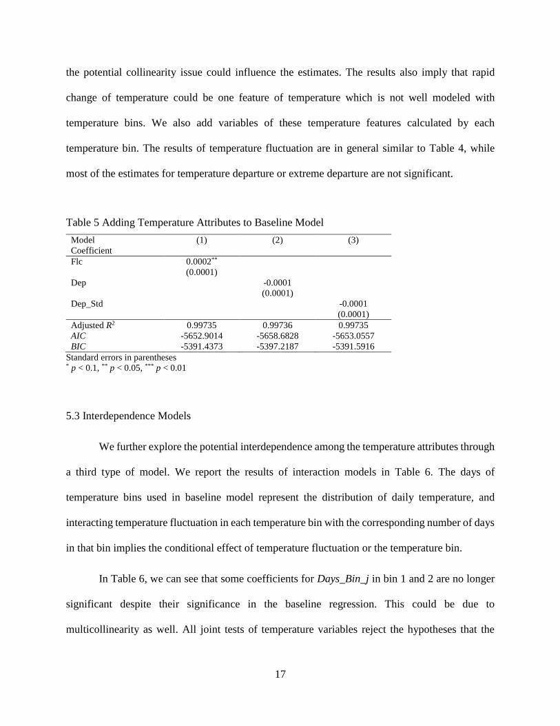
5.2 Models Including Additional Temperature Features
The results show that adding temperature attribute variables to the baseline model improves
adjusted R2, AIC and BIC (Table 5), while estimates of temperature bins are similar to those in
baseline model. Among the variables added to the baseline model, only temperature fluctuation
has a significant coefficient (Table 5). Temperature departure, regardless whether it is measured
with extreme abnormality or not, is not significant, although the AICs and BICs of the two models
including either one of the two measurements of temperature abnormality are better than those in
the baseline model. While the joint test of temperature bins and each of the added variables rejects
the null hypothesis that the coefficients are jointly zero, variance inflation factors (VIFs) suggest
the potential issue of multicollinearity among temperature bins and the added temperature variable.
These results suggest the improvement by capturing more features of temperature, even though
17
the potential collinearity issue could influence the estimates. The results also imply that rapid
change of temperature could be one feature of temperature which is not well modeled with
temperature bins. We also add variables of these temperature features calculated by each
temperature bin. The results of temperature fluctuation are in general similar to Table 4, while
most of the estimates for temperature departure or extreme departure are not significant.
Table 5 Adding Temperature Attributes to Baseline Model
Model
Coefficient
(1) (2) (3)
Flc 0.0002**
(0.0001)
Dep
-0.0001
(0.0001)
Dep_Std
-0.0001
(0.0001)
Adjusted R2 0.99735 0.99736 0.99735
AIC -5652.9014 -5658.6828 -5653.0557
BIC -5391.4373 -5397.2187 -5391.5916
Standard errors in parentheses * p < 0.1, ** p < 0.05, *** p < 0.01
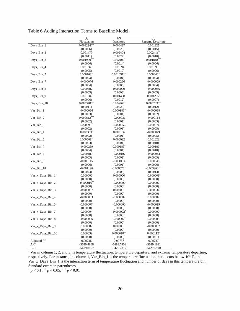
5.3 Interdependence Models
We further explore the potential interdependence among the temperature attributes through
a third type of model. We report the results of interaction models in Table 6. The days of
temperature bins used in baseline model represent the distribution of daily temperature, and
interacting temperature fluctuation in each temperature bin with the corresponding number of days
in that bin implies the conditional effect of temperature fluctuation or the temperature bin.
In Table 6, we can see that some coefficients for Days_Bin_j in bin 1 and 2 are no longer
significant despite their significance in the baseline regression. This could be due to
multicollinearity as well. All joint tests of temperature variables reject the hypotheses that the
18
coefficients are jointly zero. For temperature fluctuation, its coefficients in bin 2 to bin 5 are
significant and positive, while interaction terms of temperature fluctuation and the corresponding
bins are both negative. The coefficients of interaction terms are significant for bin 2 and bin 5,
suggesting the existence of interdependence. Therefore, in cooler days (< 50o F), while a rapid
increase of temperature within two days leads to more residential energy consumption, more days
in the corresponding temperature bin hamper the fluctuation effect slightly. In other words, when
humans’ non-linear thermal sensation leads to more energy consumption, more days of similar
temperature, restricted within the 10o F bin, decreases the fluctuation effect, as it implies a
relatively more stable temperature within a year. The positive coefficients of temperature
fluctuation in bins with lower temperature seem to be counterintuitive, as it suggests that rapid
increase of temperature in colder days actually results in more residential energy consumption.
While the D&G’s data set has no information about what the uses of the energy, we cannot verify
if this positive effect is due to cooling demand as people have heat illusion2 or they experience the
illusion as unbearable cold and take defensive action by using heat. We should keep in mind that
in this model, the marginal effect of temperature fluctuation is not constant and depends on days
of the corresponding bin. When the number of days is larger than 38 days, the marginal effect of
rapid temperature increase is positive. Therefore, when the small range of temperature occurs more
frequently, a rapid increase of temperature in such a relatively stable weather still results in
increased energy use.
The interaction model of extreme temperature departure and days in bins tells a slightly
different story, which consistently demonstrates the complex effects of temperature. Similar to the
2 A similar example is that, when skin temperature is quite low, flushing skin with water of a bit higher temperature
than the skin often leads to a strong but mistaken sensation that the water is hot. This illusion may cause some
people to take action to warm up.
19
results in Table 4, most of the temperature departure and extreme departure coefficients in the
lower temperature bins are negative. These coefficients are not significant, possibly due to
multicollinearity. The interaction terms of temperature departure or extreme temperature departure
with number of days have a similar explanation. We thus focus on results of extreme departure as
it captures abnormality without counting normal variation of temperature.
The coefficients of the interaction terms are negative in colder bins (i.e., bin 1 and bin 3),
which suggests that, conditional on same number of days in the temperature bin, a warmer
departure from long term trend contributes to less residential energy consumption in cold days and
a colder departure further increases the consumption in addition to the absolute temperature level.
Similarly, the positive coefficient (0.0001) in of the interaction term in bin 10 suggests that, when
the absolute temperature level is above 90o F, extreme temperature departure leads to further
consumption of residential energy.
The negative coefficient of extreme departure in bin 10 (-0.004) seems counterintuitive at
first glance. Yet, as the coefficient of its interaction term with days of that bin is significant, it
suggests the interdependence. The marginal effect of this extreme departure of hot days can lead
to either more or less energy consumption, because of inverse sign of the coefficient for that
interaction term. Therefore, when temperature is high but total hot days in bin 10 (> 90o F) in a
year is less than 35, heatt abnormality leads to less residential energy consumption. But if hot days
within bin 10 occur more frequently, heat departure from long term trend results in additional
residential energy consumption. Together, these results suggest that, when temperature is hotter
than its long term trend, households’ adaptation activities are conditional on how frequently the
hot days occur, regardless whether it is usual or not.
20
Table 6 Adding Interaction Terms to Baseline Model
(1) (2) (3)
Fluctuation Departure Extreme Departure
Days_Bin_1 0.003214*** (0.0006)
0.000487 (0.0023)
0.001825 (0.0015)
Days_Bin_2 0.001479
(0.0011)
0.002404
(0.0022)
0.002411**
(0.0010) Days_Bin_3 0.001989***
(0.0006)
0.002409*
(0.0014)
0.001848***
(0.0006)
Days_Bin_4 0.001037** (0.0005)
0.001694* (0.0010)
0.001398** (0.0006)
Days_Bin_5 0.000763**
(0.0004)
0.001091***
(0.0004)
0.000840**
(0.0004) Days_Bin_7 -0.000076
(0.0004)
0.000266
(0.0006)
-0.000029
(0.0004)
Days_Bin_8 0.000382 (0.0005)
0.000009 (0.0008)
-0.000046 (0.0005)
Days_Bin_9 0.001534**
(0.0006)
0.001498
(0.0012)
0.001205*
(0.0007) Days_Bin_10 0.003348***
(0.0011)
0.004269*
(0.0023)
0.003233***
(0.0012)
Var_Bin_1+ -0.000086 (0.0003)
-0.000186** (0.0001)
-0.000098 (0.0002)
Var_Bin_2 0.000612***
(0.0002)
-0.000036
(0.0001)
-0.000114
(0.0003) Var_Bin_3 0.000393**
(0.0002)
-0.000056
(0.0001)
0.000674
(0.0005) Var_Bin_4 0.000353*
(0.0002)
0.000156
(0.0001)
-0.000079
(0.0005)
Var_Bin_5 0.000561** (0.0003)
0.000022 (0.0001)
0.001622 (0.0010)
Var_Bin_7 -0.000239
(0.0004)
0.000185*
(0.0001)
0.000186
(0.0010) Var_Bin_8 0.000489
(0.0003)
-0.000107
(0.0001)
-0.000043
(0.0005)
Var_Bin_9 -0.000145 (0.0006)
-0.000114 (0.0001)
0.000646 (0.0006)
Var_Bin_10 -0.001196
(0.0023)
-0.000576**
(0.0003)
-0.003968***
(0.0013) Var_x_Days_Bin_1+ 0.000006
(0.0000)
0.000000
(0.0000)
-0.000009*
(0.0000)
Var_x_Days_Bin_2 -0.000016** (0.0000)
-0.000000 (0.0000)
0.000007 (0.0000)
Var_x_Days_Bin_3 -0.000007
(0.0000)
0.000001
(0.0000)
-0.000034*
(0.0000) Var_x_Days_Bin_4 -0.000003
(0.0000)
-0.000002
(0.0000)
0.000007
(0.0000)
Var_x_Days_Bin_5 -0.000007* (0.0000)
-0.000000 (0.0000)
-0.000019 (0.0000)
Var_x_Days_Bin_7 0.000004
(0.0000)
-0.000002*
(0.0000)
0.000000
(0.0000) Var_x_Days_Bin_8 -0.000006
(0.0000)
0.000002*
(0.0000)
0.000003
(0.0000)
Var_x_Days_Bin_9 0.000002 (0.0000)
0.000001 (0.0000)
-0.000007 (0.0000)
Var_x_Days_Bin_10 0.000039
(0.0000)
0.000010**
(0.0000)
0.000112*
(0.0001)
Adjusted R2 0.99736 0.99737 0.99737
AIC -5680.4808 -5688.7458 -5689.1631
BIC -5419.0167 -5427.2817 -5427.6990 + Var in column 1, 2, and 3, is temperature fluctuation, temperature departure, and extreme temperature departure,
respectively. For instance, in column 1, Var_Bin_1 is the temperature fluctuation that occurs below 10o F, and
Var_x_Days_Bin_1 is the interaction term of temperature fluctuation and number of days in this temperature bin.
Standard errors in parentheses * p < 0.1, ** p < 0.05, *** p < 0.01
21
6. Discussion and Conclusion
Using D&G’s data set and empirical model, but adding strategies for capturing alternative
and additional temperature attributes, our work discuss potentially ignored features of temperature
and the complexity of temperature effects on energy consumption. Our results show that, in models
capturing a single temperature attribute, popularly used temperature bin strategy provides better
explanatory power according to the adjusted R2, AIC and BIC. However, the significance of the
alternative temperature variables other than temperature bins suggests omitted temperature
attributes when empirical models include variables such as temperature bins which capture only
absolute temperature level. By adding a variable capturing additional temperature attribute to the
baseline model using temperature bins, we further explore if these additional attributes contribute
to the analysis of temperature effects. The results suggest an improvement in explanatory power
in comparison to the baseline model. In particular, variables measuring rapid temperature change
may capture the influence of temperature not identified by temperature bins. While the positive
coefficient of temperature fluctuation implies additional residential energy consumption from
absolute temperature level, omitting non-linear human sensation of short term temperature change
may produce models that suffer from biased estimates and prediction.
We further explore the potential complexity of temperature effects through interaction
terms between distribution of absolute temperature level and the alternative temperature attributes.
The results suggest that, for some ranges of temperature levels, the effect of temperature
fluctuation or extreme temperature departure do depends on the days in the corresponding bins.
Yet, the results and implication of the two types of attributes are different. If the temperature is
less than 50o F, the rapid temperature increase results in more residential energy consumption.
While nonlinear thermal sensation suggests a stronger hot feeling from such temperature change,
22
due to data limitations, we cannot further verify the increase in energy consumption is for cooling
due to heat illusion or for heating. But more days with similar temperature hampers the fluctuation
effect, which could be due to that fact that humans adjust to the stimulus of rapid temperature
change if similar temperatures occur often, such that people perceive the weather as stable.
Similarly, the more dramatic the rapid increase, the smaller marginal effect of colder temperature
bins could be on increasing energy consumption, which is consistent with non-linear thermal
sensation.
The results of the interaction model including extreme temperature departure, days of
temperature bins, and their interaction terms, demonstrate more complicated temperature effects
in hot days, which are somewhat counterintuitive, while the effect of temperature abnormality is
straightforward in cold days. When temperature level is low (e.g., bin 1), warmer abnormality
results in less residential energy consumption, as households are used to normally even lower
temperature in the long term. The coefficients of abnormality in hot temperature (i.e., bin 10, >
90o F) are negative. It indicates less energy consumption when temperature should be cooler than
usual but is actually hotter. Taking the interaction term into consideration, the marginal effect of
temperature abnormality in hot days depends on the frequency of temperature in bin 10. Our results
suggest that, households have different responses to adapt hot abnormality conditional on the
frequency of hot days. If a year has more than 35 hot days ( > 90o F), households appear to respond
to extreme hot abnormality through alternative actions not associated with residential energy
consumption. But if such hot days are more frequent in the year, then households’ adaptation to
heat abnormality results in more residential energy consumption. While heat abnormality
represents the departure of temperature from long term trend, households may not invest in air
conditioning if normal temperature is not that hot and in the abnormal year hot days are infrequent.
23
Our findings also have policy implications. In the context of climate change and global
warming, our findings suggest that abnormal weather may not always lead to more energy
consumption, which is somewhat different than the findings in received literature. Abnormally hot
weather in the cold days reduces energy consumption, and its effect in the hot days could either
decrease or increase residential energy consumption, depending on the frequency of hot days of
the year. In the long term, climate change may not necessarily lead to more residential air
conditioning energy demand, if climate change is associated with larger variation in temperature.
Residential energy policies aiming to respond climate change need to be reviewed if they adopt
the assumptions based on non-conditional relationships between temperature abnormality and
energy consumption.
Through the discussion of three types of model specification, our study provides a more
complete understanding of complex temperature effects on residential energy consumption and
suggests ways to improve the effectiveness of related research methods. Our analysis of
interdependence and abnormality further demonstrates the existence of complex temperature
effects on energy consumption. These findings may also contribute to energy supply management
and power plant construction policies in the context of climate change in which there could be
more variations in temperature in addition to warmer annual temperature, or even simply to better
forecast power needs in the short term. According to our findings, empirical models discussing
temperature effects on energy consumption may consider including temperature variables in
addition to the conventional CHDD or temperature bins. The inclusion of interdependence among
temperature attributes may also help to explain the influences of abnormal temperature instead of
the comparison of historical temperature data and forecasted temperature data. While our analysis
provides some insights into the relationship between temperature and market outcomes, the
24
analysis of complex temperature effects requires further efforts to better deal with potential
multicollinearity and to understand the positive correlation between temperature fluctuation and
low temperature.
25
References
Albouy, David, Walter Graf, Ryan Kellogg, and Hendrik Wolff. 2013. Climate amenities, climate
change, and American quality of life. National Bureau of Economic Research.
Arens, Edward, Hui Zhang, and Charlie Huizenga. 2006. "Partial- and whole-body thermal
sensation and comfort—Part II: Non-uniform environmental conditions." Journal of
Thermal Biology 31 (1–2):60-66. doi: http://dx.doi.org/10.1016/j.jtherbio.2005.11.027.
Auffhammer, Maximilian, and Anin Aroonruengsawat. 2011. "Simulating the impacts of climate
change, prices and population on California’s residential electricity consumption."
Climatic Change 109 (1):191-210. doi: 10.1007/s10584-011-0299-y.
Brooks, Jeremy, Douglas Oxley, Arnold Vedlitz, Sammy Zahran, and Charles Lindsey. 2014.
"Abnormal Daily Temperature and Concern about Climate Change Across the United
States." Review of Policy Research 31 (3):199-217. doi: 10.1111/ropr.12067.
Brulle, Robert J., Jason Carmichael, and J. Craig Jenkins. 2012. "Shifting public opinion on climate
change: an empirical assessment of factors influencing concern over climate change in the
U.S., 2002–2010." Climatic Change 114 (2):169-188. doi: 10.1007/s10584-012-0403-y.
Buhaug, Halvard. 2010. "Climate not to blame for African civil wars." Proceedings of the
National Academy of Sciences 107 (38):16477-16482. doi: 10.1073/pnas.1005739107.
Burke, Marshall B., Edward Miguel, Shanker Satyanath, John A. Dykema, and David B. Lobell.
2009. "Warming increases the risk of civil war in Africa." Proceedings of the National
Academy of Sciences 106 (49):20670-20674. doi: 10.1073/pnas.0907998106.
Cao, Melanie, and Jason Wei. 2005. "Stock market returns: A note on temperature anomaly."
Journal of Banking & Finance 29 (6):1559-1573. doi: 10.1016/j.jbankfin.2004.06.028.
Considine, Timothy J. 2000. "The impacts of weather variations on energy demand and carbon
emissions." Resource and Energy Economics 22 (4):295-314. doi:
http://dx.doi.org/10.1016/S0928-7655(00)00027-0.
De Cian, Enrica, Elisa Lanzi, and Roberto Roson. 2013. "Seasonal temperature variations and
energy demand." Climatic Change 116 (3):805-825. doi: 10.1007/s10584-012-0514-5.
De Cian, Enrica, and Ian Sue Wing. 2016. "Global Energy Demand in a Warming Climate."
de Dear, R. J., J. W. Ring, and P. O. Fanger. 1993. "Thermal Sensations Resulting From Sudden
Ambient Temperature Changes." Indoor Air 3 (3):181-192. doi: 10.1111/j.1600-
0668.1993.t01-1-00004.x.
Deschênes, Olivier, and Michael Greenstone. 2011. "Climate Change, Mortality, and Adaptation:
Evidence from Annual Fluctuations in Weather in the US." American Economic Journal:
Applied Economics 3 (4):pp.-152-185.
Deschênes, Olivier, Michael Greenstone, and Jonathan Guryan. 2009. "Climate Change and Birth
Weight." The American Economic Review 99 (2):211-217.
Egan, Patrick J., and Megan Mullin. 2012. "Turning personal experience into political attitudes:
the effect of local weather on Americans’ perceptions about global warming." The Journal
of Politics 1 (1):1-14.
26
Eskeland, Gunnar S., and Torben K. Mideksa. 2010. "Electricity demand in a changing climate."
Mitigation and Adaptation Strategies for Global Change 15 (8):877-897. doi:
10.1007/s11027-010-9246-x.
Fikru, Mahelet G., and Luis Gautier. 2015. "The impact of weather variation on energy
consumption in residential houses." Applied Energy 144:19-30. doi:
http://dx.doi.org/10.1016/j.apenergy.2015.01.040.
Hamilton, Lawrence C., and Mary D. Stampone. 2013. "Blowin’ in the Wind: Short-Term Weather
and Belief in Anthropogenic Climate Change." Weather, Climate, and Society 5 (2):112-
119. doi: 10.1175/WCAS-D-12-00048.1.
Jacobsen, Ben, and Wessel Marquering. 2008. "Is it the weather?" Journal of Banking & Finance
32:526-540. doi: 10.1016/j.jbankfin.2007.08.004.
Jacobsen, Ben, and Wessel Marquering. 2009. "Is it the weather? Response." Journal of Banking
& Finance 33:583-587. doi: 10.1016/j.jbankfin.2008.09.011.
Kamstra, Mark J., Lisa A. Kramer, and Maurice D. Levi. 2003. "Winter Blues: A SAD Stock
Market Cycle." The American Economic Review 93 (1):324-343.
Kaufmann, Robert K., Sucharita Gopal, Xiaojing Tang, Steve M. Raciti, Paul E. Lyons, Nick
Geron, and Francis Craig. 2013. "Revisiting the weather effect on energy consumption:
Implications for the impact of climate change." Energy Policy 62:1377-1384. doi:
http://dx.doi.org/10.1016/j.enpol.2013.07.056.
Lee, Gi-Eu. 2015. "Essays in State-Level Climate Change Policies." Doctoral Dissertation,
Department of Agricultural, Food, and Resource Economics, Michigan State University.
Lee, Gi-Eu, and Scott Loveridge. 2016. “Mitigation or a Vicious Circle? An Empirical Analysis
of Abnormal Temperature Effects on Residential Electricity Consumption.” Unpublished
Work, Michigan State University.
Lee, Gi-Eu, Scott Loveridge, and Julie A Winkler. 2016. "Does the Public Care About How
Climate Change Might Affect Agriculture?" Choices 31 (1):1-5.
Li, Y. 2005. "Perceptions of temperature, moisture and comfort in clothing during environmental
transients." Ergonomics 48 (3):234-248. doi: 10.1080/0014013042000327715.
Lindsey, Charles, and Simon Sheather. 2010. "Variable selection in linear regression." Stata
Journal 10 (4):650.
Mansur, Erin T., Robert Mendelsohn, and Wendy Morrison. 2008. "Climate change adaptation: A
study of fuel choice and consumption in the US energy sector." Journal of Environmental
Economics & Management 55 (2):175-193. doi: 10.1016/j.jeem.2007.10.001.
Marquart-Pyatt, Sandra T., Aaron M. McCright, Thomas Dietz, and Riley E. Dunlap. 2014.
"Politics eclipses climate extremes for climate change perceptions." Global Environmental
Change 29:246-257. doi: http://dx.doi.org/10.1016/j.gloenvcha.2014.10.004.
Mideksa, Torben K., and Steffen Kallbekken. 2010. "The impact of climate change on the
electricity market: A review." Energy Policy 38 (7):3579-3585. doi:
http://dx.doi.org/10.1016/j.enpol.2010.02.035.
27
Quayle, Robert G., and Henry F. Diaz. 1980. "Heating Degree Day Data Applied to Residential
Heating Energy Consumption." Journal of Applied Meteorology 19 (3):241-246. doi:
10.1175/1520-0450(1980)019<0241:HDDDAT>2.0.CO;2.
Savić, Stevan, Aleksandar Selakov, and Dragan Milošević. 2014. "Cold and warm air temperature
spells during the winter and summer seasons and their impact on energy consumption in
urban areas." Natural Hazards 73 (2):373-387. doi: 10.1007/s11069-014-1074-y.
Scruggs, Lyle, and Salil Benegal. 2012. "Declining public concern about climate change: Can we
blame the great recession?" Global Environmental Change 22 (2):505-515. doi:
http://dx.doi.org/10.1016/j.gloenvcha.2012.01.002.
Uri, Noel D. 1986. "The Demand for Beverages and Interbeverage Substitution in the United
States." Bulletin of Economic Research 38:77-85. doi: 10.1111/j.1467-
8586.1986.tb00204.x.
Wang, Zhe, Zhen Zhao, Borong Lin, Yingxin Zhu, and Qin Ouyang. 2015. "Residential heating
energy consumption modeling through a bottom-up approach for China's Hot Summer–
Cold Winter climatic region." Energy and Buildings 109:65-74. doi:
http://dx.doi.org/10.1016/j.enbuild.2015.09.057.
Zaval, Lisa, Elizabeth A. Keenan, Eric J. Johnson, and Elke U. Weber. 2014. "How warm days
increase belief in global warming." Nature Climate Change 4 (2):143-147. doi:
10.1038/nclimate2093.