Temperature of the inner-core boundary of the Earth: Melting of iron at high pressure fromfirst-principles coexistence simulations
Dario Alfè*Department of Earth Sciences and Department of Physics and Astronomy, Materials Simulation Laboratory,
and London Centre for Nanotechnology, UCL, Gower Street, London WC1E 6BT, United Kingdom�Received 11 December 2008; published 11 February 2009�
The Earth’s core consists of a solid ball with a radius of 1221 Km, surrounded by a liquid shell whichextends up to 3480 km from the center of the planet, roughly half way toward the surface �the mean radius ofthe Earth is 6373 km�. The main constituent of the core is iron, and therefore the melting temperature of ironat the pressure encountered at the boundary between the solid and the liquid �the inner-core boundary �ICB��provides an estimate of the temperature of the core. Here I report the melting temperature of Fe at pressuresnear that of the ICB, obtained with first-principles techniques based on density-functional theory. The calcu-lations have been performed by directly simulating solid and liquid iron in coexistence and show that and at apressure of �328 GPa iron melts at �6370�100 K. These findings are in good agreement with earliersimulations, which used exactly the same quantum-mechanics techniques but obtained melting properties fromthe calculation of the free energies of solid and liquid Fe.
The study of iron under extreme conditions has a longhistory. In particular, numerous attempts have been made toobtain its high-pressure melting properties.1–9 Experimen-tally, Earth’s core conditions can only be reproduced byshock wave �SW� experiments in which a high-speed projec-tile is fired at an iron sample, and upon impact high-pressureand high-temperature conditions are produced. By varyingthe speed of the projectile it is possible to investigate a char-acteristic pressure-volume relation known as the Hugoniot10
and even infer temperatures, although a word of caution hereis in order as temperature estimates are often based on theknowledge of quantities such as the constant volume specificheat and the Grüneisen parameter, which are only approxi-mately known at the relevant conditions.7 If the speed of theprojectile is high enough, the conditions of pressure and tem-perature are such that the sample melts, and it is thereforepossible to obtain points on the melting curve, of course withthe caveat mentioned above about temperature measure-ments. An alternative route to high-pressure, high-temperature properties is the use of diamond anvil cells�DAC� in which the sample is surrounded by a pressure me-dium and statically compressed between two diamond anvils.In DAC experiments pressure and temperatures can be di-rectly measured, and therefore these techniques should inprinciple be more reliable to investigate melting properties.Unfortunately, in the case of iron it is not so and there is afairly large range of results obtained by different groups.1–6
An alternative approach used for the past ten years or sohas been to employ theory—and in particular quantum-mechanics techniques based on density-functional theory�DFT�—to calculate the high-pressure melting curve of iron.A number of groups have used different approaches to theproblem. Our own strategy has been to calculate the Gibbsfree energy of solid and liquid iron and then obtain the melt-ing curve by imposing their equality for any fixed pressure.We obtained a melting temperature of �6350 K at 330GPa.11 The approach of Belonoshko et al.12 was to fit anembedded atom model �EAM� to first-principles calculations
and then calculate the melting curve of the EAM. They ob-tained a temperature of �7050 K at 330 GPa. The approachof Laio et al.13 was similar, although they refitted their opti-mized potential model �OPM� to first-principles calculationsin a self-consistent way. They obtained a melting tempera-ture of �5400 K at 330 GPa. We later reconciled the resultsof Belonoshko et al.12 with ours by showing that the differ-ence was due to a difference in free energies between theirEAM and our DFT.14 A similar argument would be respon-sible for the difference between our results and those of Laioet al.13
Here I am using an approach to melting which is indepen-dent of the free-energy technique used earlier,11,15,16 and themain motivation of this work is to provide an alternativeroute to the calculation of the melting properties of Fe. Themethod employed here is that of the coexistence of phases inwhich solid and liquid iron are simulated in coexistence. Thefirst time that the method was used in the context of first-principles calculations was for the low-pressure meltingcurve of aluminum,17 where it was shown to deliver the sameresults as the free-energy method.18 It was later applied tocompute the melting curve of LiH,19 hydrogen,20 and MgO.21
The coexistence method is intrinsically expensive as itrequires large simulation cells and long simulations. It can beapplied in a number of different ways. Here I have used theNVE ensemble, i.e., constant number of atoms N, constantvolume V, and constant internal energy E. In the NVE en-semble, for each chosen volume V there is a whole range ofenergies E for which solid and liquid can coexist for a longtime; the average temperature and pressure along the simu-lation then provide a point on the melting curve. If the en-ergy E is above �below� the range where coexistence can bemaintained, the system will completely melt �solidify�, andthe simulation does not provide useful melting propertiesinformation. It should be pointed out that any finite systemwill eventually melt or solidify if simulated for long enoughdue to spontaneous fluctuations. However, melting �solidifi-
cation� resulting from a too-high �low� value of E typicallyappears on much shorter time scales.
The present calculations have been performed withdensity-functional theory with the generalized gradient ap-proximation known as PW91 �Ref. 22� and the projectoraugmented wave method23,24 as implemented in the VASPcode.25 An efficient extrapolation of the charge density wasemployed.26 Single-particle orbitals were expanded in planewaves with a cutoff of 300 eV, and I used the finite tempera-ture implementation of DFT as developed by Mermin.27
These settings are exactly equivalent to those used in ourprevious work,11,15,16 so the melting properties obtained herewill be directly comparable to those early ones. The simula-tions have been performed on hexagonal closed packed �hcp�cells containing 980 atoms �7�7�10�, using the � pointonly. For the temperatures of interest here the use of the �point provides completely converged results. The time stepin the molecular-dynamics simulations was 1 fs, and the self-consistency on the total energy was 2�10−5 eV. With theseprescriptions the drift in the constant of motion was�0.5 K /ps.
The coexistence simulations were prepared by startingfrom a perfect hcp crystal, which was initially thermalized to�6300 K for 1 ps. Then half of the atoms in the cell wereclamped and the temperature was raised to a very high valueto melt the other half of the cell. Once good melt was ob-tained, the temperature was reduced back to 6300 K and thesystem thermalized for one additional ps, after which thesimulation was stopped, new initial velocities were assignedto the atoms, and the simulation continued in the microca-nonical ensemble. The simulations were monitored using thedensity profile, calculated by dividing the simulation cell in100 slices parallel to the solid-liquid interface and countingthe number of atoms in each slice; in the solid region this isa periodic function, with large number of atoms if the slicecoincides with an atomic plane, and small values if it fallsbetween atomic layers. In the liquid region it fluctuates ran-domly around some average value.
I performed five different simulations, starting with differ-ent amounts of internal energies E provided to the system byassigning different initial velocities to the atoms. The simu-lation with the highest value of E completely melted after�6 ps. The one with the lowest amount of E solidified after�11 ps. Among the other three, one melted after �14 ps,one after �24 ps, while the last one has remained in coex-istence for the whole length of �25 ps. However, most of
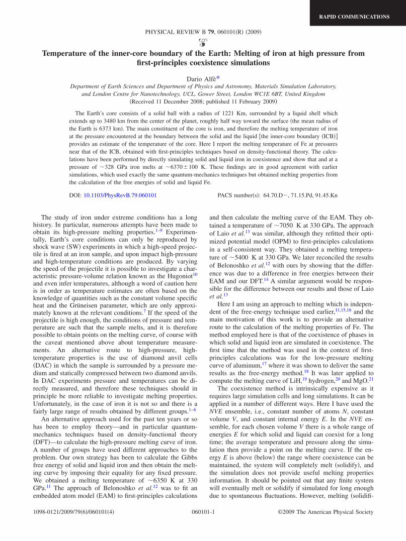
these simulations were coexisting for long enough so thatuseful melting information from the period of coexistencecould actually be extracted in almost all cases. A snapshot ofa simulation with solid and liquid in coexistence is show inFig. 1.28
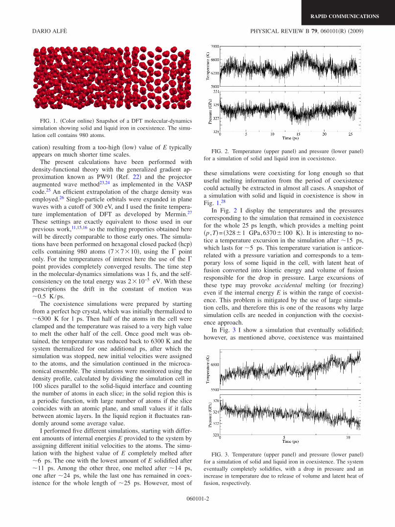
In Fig. 2 I display the temperatures and the pressurescorresponding to the simulation that remained in coexistencefor the whole 25 ps length, which provides a melting point�p ,T�= �328�1 GPa,6370�100 K�. It is interesting to no-tice a temperature excursion in the simulation after �15 ps,which lasts for �5 ps. This temperature variation is anticor-related with a pressure variation and corresponds to a tem-porary loss of some liquid in the cell, with latent heat offusion converted into kinetic energy and volume of fusionresponsible for the drop in pressure. Large excursions ofthese type may provoke accidental melting �or freezing�even if the internal energy E is within the range of coexist-ence. This problem is mitigated by the use of large simula-tion cells, and therefore this is one of the reasons why largesimulation cells are needed in conjunction with the coexist-ence approach.
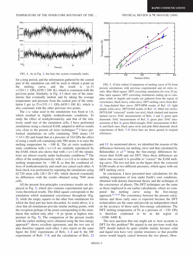
In Fig. 3 I show a simulation that eventually solidified;however, as mentioned above, coexistence was maintained
FIG. 1. �Color online� Snapshot of a DFT molecular-dynamicssimulation showing solid and liquid iron in coexistence. The simu-lation cell contains 980 atoms.
FIG. 2. Temperature �upper panel� and pressure �lower panel�for a simulation of solid and liquid iron in coexistence.
FIG. 3. Temperature �upper panel� and pressure �lower panel�for a simulation of solid and liquid iron in coexistence. The systemeventually completely solidifies, with a drop in pressure and anincrease in temperature due to release of volume and latent heat offusion, respectively.
DARIO ALFÈ PHYSICAL REVIEW B 79, 060101�R� �2009�
RAPID COMMUNICATIONS
060101-2
for a long period, and the information gathered by the centralpart of the simulation can still be used to obtain a point onthe melting curve, and the result is �p ,T�= �324�1 GPa,6250�100 K�, which is consistent with theprevious point. Similarly, in Fig. 4 I show one of the simu-lations that eventually melted, and by taking the averagetemperature and pressure from the central part of the simu-lation I get �p ,T�= �331�1 GPa,6430�100 K�, which isalso consistent with the other previous two points.
The c /a value used in the simulations was fixed at 1.6,which resulted in slightly nonhydrostatic conditions. Tostudy the effect of nonhydrostaticity, and that of the rela-tively small size of the simulation cells, I have performedsimulations using a classical EAM, adapted to deliver resultsvery close to the present ab initio techniques.14 I have per-formed simulations on cells containing 7840 atoms �14�14�20� and found that at a pressure of 324 GPa the effectof using a small cell containing only 980 atoms is to raise themelting temperature by �100 K. The ab initio nonhydro-static conditions with c /a=1.6 are similarly reproduced bythe EAM, which also shows that with c /a=1.65 the simula-tions are almost exactly under hydrostatic conditions.29 Theeffect of the nonhydrostaticity with c /a=1.6 is to reduce themelting temperature by �100 K so that the combined ef-fects of nonhydrostaticity and small size cancel each other. Afinal check was performed by repeating the simulations using62 720 atom cells �28�28�40�, which showed essentiallyno differences with the results obtained using 7840 atomcells.
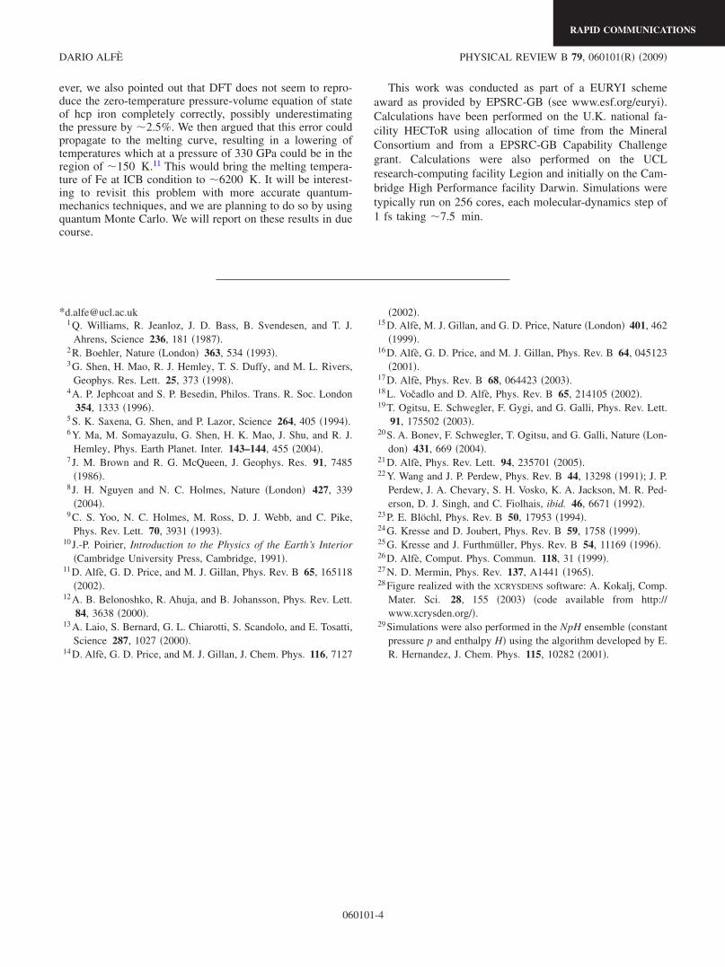
All the present first-principles coexistence results are dis-played in Fig. 5, which also contains experimental and pre-vious theoretical results. The filled square corresponds to thesimulation which maintained coexistence throughout �Fig.2�, while the empty squares to the other four simulations forwhich the final part has been discarded. As noted above, it isclear that all simulations provide similar melting points, withthe exception perhaps of the point corresponding to the simu-lation that melted only after �6 ps �point at highest tem-perature in Fig. 5�. The comparison of the present resultswith the earlier melting curve obtained using the free-energyapproach11 shows excellent agreement, and the two sets ofdata therefore support each other. I also report on the samefigure the DAC experiments of Refs. 1–4 and 6, the SWexperiments of Refs. 7–9, and the calculations of Refs. 12
and 13. As mentioned above, we identified the reasons of thedifferences between our melting curve and that calculated byBelonoshko et al.12 being the free-energy differences be-tween their EAM and our DFT. Once these differences aretaken into account it is possible to “correct” the EAM melt-ing curve. The two red dots on the figure show the correctedEAM results at two different pressures, which agree with ourDFT melting curve.
In conclusion, I have presented here calculations for themelting temperature of iron under Earth’s core conditions,obtained with density-functional theory and the technique ofthe coexistence of phases. The DFT techniques are the sameas those employed in our earlier calculations, where we com-puted the melting curve using the free-energyapproach.11,15,16 The consistency between the present calcu-lations and those early ones is expected because the DFTtechnicalities are the same and provide an independent checkon the accuracy of those early free-energy calculations. TheDFT melting temperature of Fe at a pressure of �330 GPais therefore confirmed to be in the region of�6300–6400 K.
The next question that one might ask is: how accurate isDFT for this problem? We argued in our previous work thatDFT should indeed be quite reliable mainly because solidand liquid iron have very similar structures so that possibleerrors would largely cancel between the two phases. How-
FIG. 4. As in Fig. 3, but here the system eventually melts.
FIG. 5. �Color online� Comparison of melting curve of Fe frompresent calculations with previous experimental and ab initio re-sults. Blue filled square: DFT coexisting simulation for over 25 ps;blue open squares: DFT coexisting simulations ending up to com-plete solids or liquids and results are gathered from the region ofcoexistence; black heavy solid curve: DFT melting curve from Ref.11; long-dashed blue curve: DFT-OPM results of Ref. 13; lightpurple solid curve: DFT-EAM results of Ref. 12; filled red circles:DFT-EAM “corrected” results �see text�; black chained and maroondashed curves: DAC measurements of Refs. 1 and 2; green opendiamonds: DAC measurements of Ref. 3; green plus: DAC mea-surement of Ref. 6; green filled triangle: DAC measurement of Ref.4; and black stars, black open circle and pink filled diamond: shockexperiments of Refs. 7–9. Error bars are those quoted in originalreferences.
TEMPERATURE OF THE INNER-CORE BOUNDARY OF THE … PHYSICAL REVIEW B 79, 060101�R� �2009�
RAPID COMMUNICATIONS
060101-3
ever, we also pointed out that DFT does not seem to repro-duce the zero-temperature pressure-volume equation of stateof hcp iron completely correctly, possibly underestimatingthe pressure by �2.5%. We then argued that this error couldpropagate to the melting curve, resulting in a lowering oftemperatures which at a pressure of 330 GPa could be in theregion of �150 K.11 This would bring the melting tempera-ture of Fe at ICB condition to �6200 K. It will be interest-ing to revisit this problem with more accurate quantum-mechanics techniques, and we are planning to do so by usingquantum Monte Carlo. We will report on these results in duecourse.
This work was conducted as part of a EURYI schemeaward as provided by EPSRC-GB �see www.esf.org/euryi�.Calculations have been performed on the U.K. national fa-cility HECToR using allocation of time from the MineralConsortium and from a EPSRC-GB Capability Challengegrant. Calculations were also performed on the UCLresearch-computing facility Legion and initially on the Cam-bridge High Performance facility Darwin. Simulations weretypically run on 256 cores, each molecular-dynamics step of1 fs taking �7.5 min.
*[email protected] Q. Williams, R. Jeanloz, J. D. Bass, B. Svendesen, and T. J.
Ahrens, Science 236, 181 �1987�.2 R. Boehler, Nature �London� 363, 534 �1993�.3 G. Shen, H. Mao, R. J. Hemley, T. S. Duffy, and M. L. Rivers,
Geophys. Res. Lett. 25, 373 �1998�.4 A. P. Jephcoat and S. P. Besedin, Philos. Trans. R. Soc. London
354, 1333 �1996�.5 S. K. Saxena, G. Shen, and P. Lazor, Science 264, 405 �1994�.6 Y. Ma, M. Somayazulu, G. Shen, H. K. Mao, J. Shu, and R. J.
Hemley, Phys. Earth Planet. Inter. 143–144, 455 �2004�.7 J. M. Brown and R. G. McQueen, J. Geophys. Res. 91, 7485
�1986�.8 J. H. Nguyen and N. C. Holmes, Nature �London� 427, 339
�2004�.9 C. S. Yoo, N. C. Holmes, M. Ross, D. J. Webb, and C. Pike,
Phys. Rev. Lett. 70, 3931 �1993�.10 J.-P. Poirier, Introduction to the Physics of the Earth’s Interior
�Cambridge University Press, Cambridge, 1991�.11 D. Alfè, G. D. Price, and M. J. Gillan, Phys. Rev. B 65, 165118
�2002�.12 A. B. Belonoshko, R. Ahuja, and B. Johansson, Phys. Rev. Lett.
84, 3638 �2000�.13 A. Laio, S. Bernard, G. L. Chiarotti, S. Scandolo, and E. Tosatti,
Science 287, 1027 �2000�.14 D. Alfè, G. D. Price, and M. J. Gillan, J. Chem. Phys. 116, 7127
�2002�.15 D. Alfè, M. J. Gillan, and G. D. Price, Nature �London� 401, 462
�1999�.16 D. Alfè, G. D. Price, and M. J. Gillan, Phys. Rev. B 64, 045123
�2001�.17 D. Alfè, Phys. Rev. B 68, 064423 �2003�.18 L. Vočadlo and D. Alfè, Phys. Rev. B 65, 214105 �2002�.19 T. Ogitsu, E. Schwegler, F. Gygi, and G. Galli, Phys. Rev. Lett.
91, 175502 �2003�.20 S. A. Bonev, F. Schwegler, T. Ogitsu, and G. Galli, Nature �Lon-
don� 431, 669 �2004�.21 D. Alfè, Phys. Rev. Lett. 94, 235701 �2005�.22 Y. Wang and J. P. Perdew, Phys. Rev. B 44, 13298 �1991�; J. P.
Perdew, J. A. Chevary, S. H. Vosko, K. A. Jackson, M. R. Ped-erson, D. J. Singh, and C. Fiolhais, ibid. 46, 6671 �1992�.
23 P. E. Blöchl, Phys. Rev. B 50, 17953 �1994�.24 G. Kresse and D. Joubert, Phys. Rev. B 59, 1758 �1999�.25 G. Kresse and J. Furthmüller, Phys. Rev. B 54, 11169 �1996�.26 D. Alfè, Comput. Phys. Commun. 118, 31 �1999�.27 N. D. Mermin, Phys. Rev. 137, A1441 �1965�.28 Figure realized with the XCRYSDENS software: A. Kokalj, Comp.
Mater. Sci. 28, 155 �2003� �code available from http://www.xcrysden.org/�.
29 Simulations were also performed in the NpH ensemble �constantpressure p and enthalpy H� using the algorithm developed by E.R. Hernandez, J. Chem. Phys. 115, 10282 �2001�.