Recommendation ITU-R P.2001-2(07/2015)

A general purpose wide-range terrestrial propagation model in the

frequency range 30 MHz to 50 GHz

P SeriesRadiowave propagation

ii Rec. ITU-R P.2001-2

Foreword

The role of the Radiocommunication Sector is to ensure the rational, equitable, efficient and economical use of the radio-frequency spectrum by all radiocommunication services, including satellite services, and carry out studies without limit of frequency range on the basis of which Recommendations are adopted.

The regulatory and policy functions of the Radiocommunication Sector are performed by World and Regional Radiocommunication Conferences and Radiocommunication Assemblies supported by Study Groups.

Policy on Intellectual Property Right (IPR)

ITU-R policy on IPR is described in the Common Patent Policy for ITU-T/ITU-R/ISO/IEC referenced in Annex 1 of Resolution ITU-R 1. Forms to be used for the submission of patent statements and licensing declarations by patent holders are available from http://www.itu.int/ITU-R/go/patents/en where the Guidelines for Implementation of the Common Patent Policy for ITU-T/ITU-R/ISO/IEC and the ITU-R patent information database can also be found.

Series of ITU-R Recommendations(Also available online at http://www.itu.int/publ/R-REC/en)

Series Title

BO Satellite deliveryBR Recording for production, archival and play-out; film for televisionBS Broadcasting service (sound)BT Broadcasting service (television)F Fixed serviceM Mobile, radiodetermination, amateur and related satellite servicesP Radiowave propagationRA Radio astronomyRS Remote sensing systemsS Fixed-satellite serviceSA Space applications and meteorologySF Frequency sharing and coordination between fixed-satellite and fixed service systemsSM Spectrum managementSNG Satellite news gatheringTF Time signals and frequency standards emissionsV Vocabulary and related subjects

Note: This ITU-R Recommendation was approved in English under the procedure detailed in Resolution ITU-R 1.

Electronic PublicationGeneva, 2015

ITU 2015

All rights reserved. No part of this publication may be reproduced, by any means whatsoever, without written permission of ITU.

Rec. ITU-R P.2001-2 1

RECOMMENDATION ITU-R P.2001-2

A general purpose wide-range terrestrial propagation model inthe frequency range 30 MHz to 50 GHz

(2012-2013-2015)

Scope

This Recommendation contains a general purpose wide-range model for terrestrial propagation which predicts path loss due to both signal enhancements and fading over effectively the range from 0% to 100% of an average year. This makes the model particularly suitable for Monte-Carlo methods, and studies in which it is desirable to use the same propagation model, with no discontinuities in its output, for signals which may be either wanted or potentially interfering. The model covers the frequency range from 30 MHz to 50 GHz, and distances from 3 km to at least 1 000 km.

The ITU Radiocommunication Assembly,

considering

a) that to support efficient use of the radio spectrum there is a need for sharing studies in which the variability of both wanted and potentially interfering signal levels should be taken into account;

b) that to plan high-performance radio systems the prediction of signal-level variability must include the small-probability tails of both fading and enhancement distributions;

c) that Monte-Carlo simulations are useful for spectrum-planning purposes,

noting

a) that Recommendation ITU-R P.528 provides guidance on the prediction of point-to-area path loss for the aeronautical mobile service for the frequency range 125 MHz to 30 GHz and the distance range up to 1 800 km;

b) that Recommendation ITU-R P.452 provides guidance on the detailed evaluation of microwave interference between stations on the surface of the Earth at frequencies above about 0.7 GHz;

c) that Recommendation ITU-R P.617 provides guidance on the prediction of point-to-point path loss for trans-horizon radio-relay systems for the frequency range above 30 MHz and for the distance range 100 to 1 000 km;

d) that Recommendation ITU-R P.1411 provides guidance on prediction for short-range (up to 1 km) outdoor services;

e) that Recommendation ITU-R P.530 provides guidance on the prediction of point-to-point path loss for terrestrial line-of-sight systems;

f) that Recommendation ITU-R P.1546 provides guidance on the prediction of point-to-area field strengths in the VHF and UHF bands based principally on statistical analyses of experimental data;

g) that Recommendation ITU-R P.1812 provides guidance on the prediction of point-to-area field strengths in the VHF and UHF bands based principally on deterministic method;

h) that Recommendation ITU-R P.844 summarizes modes of long range propagation paths that may also occur at VHF via the ionosphere,

2 Rec. ITU-R P.2001-2

recommends

that the procedure given in the Annex be used for sharing studies over the full range of signal variability, including the small-probability tails for fading and enhancement, and for Monte-Carlo simulations.

Annex

Wide-range propagation model

Description of the calculation method

1 Introduction

This Recommendation describes a radio-wave propagation method for terrestrial paths. It has a wide range of applicability in frequency, distance, and percentage time. In particular, it predicts both fading and enhancements of signal level. It is thus particularly suitable for Monte-Carlo simulations.

Attachment J describes the structure of the model, and in particular how results representing different propagation mechanisms are combined.

1.1 Applicability

The range of applicability is as follows:

Frequency: 30 MHz to 50 GHz.

Distance: The model is believed to be most accurate from about 3 km to 1 000 km. At shorter distances, the effect of clutter (buildings, trees, etc.) will tend to dominate unless the antenna heights are high enough to given an unobstructed path. There is no specific lower limit, although the path length must be greater than zero. A prediction of basic transmission loss less than 20 dB should be considered unreliable. Similarly, there is no specific maximum distance.

Percentage time: The method predicts the basic transmission loss not exceeded for a given percentage of an average year. Any percentage time can be used as an input to the model in the range 0% to 100%. This is limited in a progressive manner within the method such that the time used in the model varies from 0.00001% to 99.99999%. This internal limitation has no significant effect from 0.001% to 99.999% time.

Antenna heights: Antennas heights above ground level must be greater than zero. There is no specific maximum height above ground. The method is believed to be reliable for antenna altitudes up to 8 000 m above sea level.

1.2 Reciprocity, and the designation of terminals

The terms “transmitting antenna” and “receiving antenna”, or more briefly just “transmitter” and “receiver”, are used to distinguish the two terminals. This is convenient for the purposes of description.

Rec. ITU-R P.2001-2 3

The method, however, is symmetrical. Which terminal is designated the “transmitter” makes no difference to the result. By convention the “transmitter” is at the start of the terrain profile.

1.3 Iteration

Some parts of the method require iterative calculations. Explicit iteration procedures are described which have been found to be efficient and stable. However, these are not necessarily optimal. Other iterative methods can be used if they are shown to give very similar results.

1.4 Organization of the Recommendation

The inputs, and the symbols used to denote them, are described in § 2.

Preliminary calculations, including obtaining various radio-climatic parameters, are described in § 3. Climatic parameters, and values derived from the inputs, are listed in approximately alphabetical order of their symbols in Table 3.1. Many of these parameters are used in more than one place in the overall method, and all symbols in Table 3.1 are unique within this Recommendation.

Section 4 describes the four main sub-models into which the method is divided. The following subsections describe the calculation of these sub-models, most of which apply to a group of propagation mechanisms. These descriptions refer extensively to appendices which define various blocks of calculation. The sub-models in the wide-range propagation model (WRPM) are independent of each other and each calculates results over the range 0% to 100%.

Section 5 describes how the final prediction is obtained by combining results from the four main sub-models. The combination method takes account of the statistical correlation properties between the sub-models. Two alternative methods are given. One is appropriate when a direct calculation of the overall basic transmission loss is required for a given value of time percentage. This method involves an approximate treatment of uncorrelated statistics. The second method is appropriate when the WRPM is used within a Monte-Carlo simulator. In this case, the uncorrelated statistics can be modelled more accurately by combining the sub-models within the Monte-Carlo method.

1.5 Style of description

The method is described in a step-by-step manner, that is, expressions are given in the order in which they should be evaluated. Equations are sometimes followed by a “where”, but this is limited to a few lines. Long lists of “where”s are avoided.

Symbols appearing within the Appendices and which do not appear in Table 3.1 should be considered re-usable. They are defined close to where they are used, or cross-referenced if appropriate.

Logarithms are to the base 10 by default. That is, log(x) = log10(x). Natural logarithms where used are indicated as ln(x) = loge(x).

2 Inputs

The inputs to the model consist of a terrain profile, described in § 2.1, and other inputs described in § 2.2.

2.1 Terrain profile

A terrain profile giving heights above sea level of the Earth’s surface, whether land or water, at points along the great-circle radio path, must be available. Information is also required on the

4 Rec. ITU-R P.2001-2

distances over sea or a large body of water, and over low-lying coastal land or areas with many lakes, according to the zones defined in Attachment D, § D.1.

In principle, the terrain profile consists of arrays each having the same number of values, n, as follows:

di: distance from transmitter of i-th profile point (km) (2.1a)

hi: height of i-th profile point above sea level (m) (2.1b)

where:i: 1, 2, 3 ... n = index of the profile pointn: number of profile points.

It is convenient to define an additional array holding zone codes as part of the profile:

zi: zone code at distance di from transmitter (2.1c)

where the z values are codes representing the zones in Table D.1.

The profile points must be spaced at equal intervals of distance. Thus d1 = 0 km, and dn = d km where d is the overall length of the path. Similarly, di = (i − 1) d / (n − 1) km.

It is immaterial whether an array di is populated with distances, or whether di is calculated when needed.

There must be at least one intermediate profile point between the transmitter and the receiver. Thus n must satisfy n  3. Such a small number of points is appropriate only for short paths, less than of the order of 1 km.

Only general guidance can be given as to the appropriate profile spacing. Typical practice is a spacing in the range 50 to 250 m, depending on the source data and the nature of terrain.

However, it is stressed that equally-spaced points should be included for the complete path, even where it passes over water. Expressions in this method assume that this is so. For instance, it is not acceptable to have zero-height points only at the start and end of a section over sea when the length of the section exceeds the point spacing. Horizon points must be located taking Earth curvature into account, and omitting points in such a manner could result in the misinterpretation of a profile.

2.2 Other inputs

Table 2.2.1 lists the other inputs which must be provided by the user, in addition to the geographic information, including the terrain profile, described in § 2.1 above. The symbols and units given here apply throughout this Recommendation.

Rec. ITU-R P.2001-2 5

TABLE 2.2.1

Other inputs

Symbol Description

f (GHz) FrequencyTpol Code indicating either horizontal or vertical linear polarization

re, rn (degrees) Longitude, latitude, of receiverte, tn (degrees) Longitude, latitude, of transmitter

htg, rg (m) Height of electrical centre of transmitting, receiving antenna above ground.Tpc (%) Percentage of average year for which the predicted basic transmission loss is not

exceededGt, Gr (dBi) Gain of transmitting, receiving, antenna in the azimuthal direction of the path towards

the other antenna, and at the elevation angle above the local horizontal of the other antenna in the case of a line-of-sight (LoS) path, otherwise of the antenna’s radio horizon, for median effective Earth radius.

Longitudes and latitudes in this method are positive east and north.

2.3 Constants

Table 2.3.1 gives values of constants used in the method.

TABLE 2.3.1

Constants

Symbol Value Description

c (m/s) 2.998  108 Speed of propagationRe (km) 6 371 Average Earth radiusrland 22.0 Relative permittivity for landrsea 80.0 Relative permittivity for sea

land (S/m) 0.003 Conductivity for landsea (S/m) 5.0 Conductivity for sea

2.4 Integral digital products

Only the file versions provided with this Recommendation should be used. They are an integral part of the Recommendation. Table 2.4.1 gives details of the digital products used in the method.

6 Rec. ITU-R P.2001-2

TABLE 2.4.1

Digital products

Filename Ref. Origin Latitude (rows) Longitude (columns

First row(ºN)

Spacing(degrees)

Number of rows

First col(ºE)

Spacing(degrees)

Number of cols

DN_Median.txt § 3.4.1 P.2001 90 1.5 121 0 1.5 241DN_SupSlope.txt § 3.4.1 P.2001 90 1.5 121 0 1.5 241DN_SubSlope.txt § 3.4.1 P.2001 90 1.5 121 0 1.5 241dndz_01.txt § 3.4.2 P.453-10 90 1.5 121 0 1.5 241Esarain_Pr6_v5.txt § C.2 P.837-5 90 1.125 161 0 1.125 321Esarain_Mt_v5.txt § C.2 P.837-5 90 1.125 161 0 1.125 321Esarain_Beta_v5.txt § C.2 P.837-5 90 1.125 161 0 1.125 321h0.txt § C.2 P.839-4 90 1.5 121 0 1.5 241Surfwv_50_fixed.txt(1) Appx F P.836-4

(corrected)90 1.5 121 0 1.5 241

FoEs50.txt Appx G P.2001 90 1.5 121 0 1.5 241FoEs10.txt Appx G P.2001 90 1.5 121 0 1.5 241FoEs01.txt Appx G P.2001 90 1.5 121 0 1.5 241FoEs0.1.txt Appx G P.2001 90 1.5 121 0 1.5 241TropoClim.txt § E.2 P.2001 89.75 0.5 360 –

179.750.5 720

(1) The file “surfwv_50_fixed.txt” is a corrected version of the file “surfwv_50.txt” associated with Recommendation ITU-R P.836-4. “surfwv_50.txt” has one column less than expected according to the “surfwv_lat.txt” and “surfwv_lon.txt” files provided with the data. It has been assumed that the column corresponding to a longitude of 360° was omitted from the file, and this has been corrected in “surfwv_50_fixed.txt.

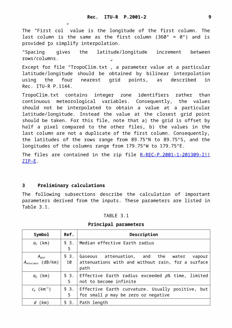
The “First row” value is the latitude of the first row.

The “First col” value is the longitude of the first column. The last column is the same as the first column (360° = 0°) and is provided to simplify interpolation.

“Spacing” gives the latitude/longitude increment between rows/columns.

Except for file “TropoClim.txt”, a parameter value at a particular latitude/longitude should be obtained by bilinear interpolation using the four nearest grid points, as described in Rec. ITU-R P.1144.

TropoClim.txt contains integer zone identifiers rather than continuous meteorological variables. Consequently, the values should not be interpolated to obtain a value at a particular latitude/longitude. Instead the value at the closest grid point should be taken. For this file, note that a) the grid is offset by half a pixel compared to the other files, b) the values in the last column are not a duplicate of the first column. Consequently, the latitudes of the rows range from 89.75°N to 89.75°S, and the longitudes of the columns range from 179.75°W to 179.75°E.

The files are contained in the zip file R-REC-P.2001-1-201309-I!!ZIP-E.

Rec. ITU-R P.2001-2 7

3 Preliminary calculations

The following subsections describe the calculation of important parameters derived from the inputs. These parameters are listed in Table 3.1.

TABLE 3.1

Principal parameters

Symbol Ref. Description

ae (km) § 3.5 Median effective Earth radiusAgsur

Awrsur,wsur (dB/km)§ 3.10 Gaseous attenuation, and the water vapour attenuations with and without

rain, for a surface pathap (km) § 3.5 Effective Earth radius exceeded p% time, limited not to become infinite

cp (km–1) § 3.5 Effective Earth curvature. Usually positive, but for small p may be zero or negative

d (km) § 3.2 Path lengthdlt,lr (km) § 3.7 Terminal to horizon distances. For LoS paths set to distances to point with

largest knife-edge lossdtcv,rcv (km) § 3.9 Terminal to troposcatter common volume distanceshcv (masl)(1) § 3.9 Height of troposcatter common volume

hhi, lo (masl)(1) § 3.3 Higher, lower, antenna heighthm (m) § 3.8 Path roughness parameter

hmid (masl)(1) § 3.2 Ground height at mid point of pathhtea, rea (m) § 3.8 Effective transmitter, receiver, heights above smooth surface for

anomalous (ducting/layer-reflection) modelhtep, rep (m) § 3.8 Effective transmitter, receiver, heights above smooth surface for

diffraction modelhts, rs (masl)(1) § 3.3 Transmitter, receiver, height above mean sea level

ilt, lr § 3.7 Profile indices of transmitter, receiver, horizonsLbfs (dB) § 3.11 Free-space basic transmission loss for the path length and frequencyLbm1 (dB) § 4.1 Basic transmission loss associated with sub-model 1, diffraction, clear-air

and precipitation fadingLbm2 (dB) § 4.2 Basic transmission loss associated with sub-model 2, anomalous

propagationLbm3 (dB) § 4.3 Basic transmission loss associated with sub-model 3, troposcatter

propagation and precipitation fadingLbm4 (dB) § 4.4 Basic transmission loss associated with sub-model 4, sporadic-E

propagationLd (dB) § 4.1 Diffraction loss not exceeded p% time

Nd1km50 (N-units) § 3.4.1 Median value of average refractivity gradient in the lowest 1 km of the atmosphere. Numerically equal to N as defined in ITU-R P.452 but with opposite sign

Nd1kmp (N-units) § 3.4.1 Average refractivity gradient in the lowest 1 km of the atmosphere exceeded for p% of an average year. Normally negative but can be zero or positive

Nd65m1 (N-units) § 3.4.2 Refractivity gradient in the lowest 65 m of the atmosphere exceeded for 1% of an average year

8 Rec. ITU-R P.2001-2

TABLE 3.1 (end)

Symbol Ref. Description

p (%) § 3.1 Percentage of average year for which predicted basic transmission loss is not exceeded, limited to range 0.00001% ≤ p ≤ 99.99999%

q (%) § 3.1 Percentage of average year for which predicted basic transmission loss is exceeded, given by 100 − p

p (mrad) § 3.3 Positive value of path inclination (m) § 3.6 Wavelength

cve, cvn (degrees) § 3.9 Troposcatter common volume longitude, latitudetcve, tcvn (degrees) § 3.9 Longitude, latitude, of mid-point of path segment from transmitter to the

troposcatter common volumercve, rcvn (degrees) § 3.9 Longitude, latitude, of mid-point of path segment from receiver to the

troposcatter common volumeme, mn (degrees) § 3.2 Path mid-point longitude, latitude

e (rad) § 3.5 Angle subtended by d km at centre of spherical Eartht, r (mrad) § 3.7 Horizon elevation angles relative to the local horizontal as viewed from

transmitter and receivertpos, rpos (mrad) § 3.7 Horizon elevation angles relative to the local horizontal limited to be

positive (not less than zero)o (dB/km) § 3.10 Sea-level specific attenuation due to oxygen

ω § 3.2 Fraction of the path over sea(1) masl: metres above sea level.

3.1 Limited percentage times

The percentage of an average year for which the predicted loss is not exceed, Tpc in Table 2.2.1, is allowed to vary from 0% to 100%. The percentage times used for calculation are limited such that they remain in the range 0.00001% to 99.99999%.

Percentage time basic transmission loss not exceeded:

p=T pc+0 .00001 ¿¿                % (3.1.1)

Percentage time basic transmission loss is exceeded:q=100−p                 % (3.1.2)

3.2 Path length, intermediate points, and fraction over sea

The path length in km is given by the last distance in the terrain profile, dn, as described in § 2.1. It is convenient to give this distance an un-subscripted symbol:

d=dn                 km (3.2.1)

Calculate the longitude and latitude of the mid-point of the path, me and mn, from the transmitter and receiver longitudes and latitudes, as given in Table 2.2.1, using the great circle path method of Attachment H by setting dpnt = 0.5 d in equation (H.3.1). Several climatic parameters are required for this location, as described below.

Rec. ITU-R P.2001-2 9

Calculate the ground height in m above sea level at the mid-point of the profile according to whether the number of profile points, n, is odd or even:

hmid=h0. 5(n+1)                 n odd     masl (3.2.2a)

hmid=0.5 (h0.5n+h0 . 5n+1)                 n even     masl (3.2.2b)

Set the fraction of the path over sea, . This fraction may be obtained from the ITU digitized world map (IDWM). If array z, described in § 2.1, has been coded according to the zones described in Attachment D, Table D.1, where adjacent z values have different codes, the boundary between the two zones should be assumed to occur half-way between the corresponding profile points.

3.3 Antenna altitudes and path inclination

The transmitter and receiver heights above sea level are calculated from the first and last terrain heights from the profile and the input heights above ground given in Table 3.1:

hts=h1+htg                 masl (3.3.1a)

hrs=hn+hrg                 masl (3.3.1b)

Assign the higher and lower antenna heights above sea level:

hhi=max (hts , hrs )                 masl (3.3.2a)

hlo=min (hts ,hrs)                 masl (3.3.2b)

The higher and lower antennas heights can be the same if hts = hrs.

Calculate the positive value of path inclination given by:

                mrad (3.3.3)

3.4 Climatic parameters

Measured values of the following climatic parameters applicable to the region concerned can be used if available. If suitable measurements are not available, the parameters can be obtained for the longitude and latitude of the mid-point of the path from data files as described in the following subsections. The files are organized as arrays of values at a fixed spacing in longitude and latitude. The first row starts at 90N and contains a full set of latitude values from 0E to 360E, even though all of these are at the North Pole. Following lines are at the point spacing further south until the South Pole is reached. The files have different point spacings, but in all cases it is sufficiently accurate to use bilinear interpolation from the four nearest data to the point required. All of these data files have associated longitude and latitude files which define the location of every point.

3.4.1 Refractivity in the lowest 1 km

The parameters Nd1km50 and Nd1kmp give the change in refractivity, in N-units, from the surface to 1 km above the surface of the Earth, not exceeded for 50% and p% of an average year respectively. These are used to account for ray bending in diffraction calculations via the concept of effective Earth radius or curvature. They can be viewed as the spatially-averaged refractivity gradient in the lowest 1 km of the atmosphere.

10 Rec. ITU-R P.2001-2

Nd1km50 is numerically equal to N, defined in Recommendations ITU-R P.452 and ITU-R P.1812, but of opposite sign. N is everywhere positive, and thus Nd1km50 is everywhere negative.

Nd1kmp can be negative or positive, depending on location and the value of p. It can fall below −157 N-units, the value at which effective Earth radius becomes infinite.

The change in sign convention adopted here is to align with a conceptually similar parameter, Nd65m1, used for clear-air multipath fading and enhancements, obtained as described in § 3.4.2 below.

Nd1km50 and Nd1kmp are available from files “DN_Median.txt”, “DN_SubSlope.txt” and “DN_SupSlope.txt”.

Obtain Nd1km50 as:

Nd 1 km50=−SdN                 N-units (3.4.1.1)

where SdN is the value interpolated from file “DN_Median.txt” for the path mid-point at me, mn.

Obtain Nd1kmp as:

Nd 1 kmp=N d 1km 50+SΔN sup log (0 .02 p )    N-units     p < 50 (3.4.1.2a)

Nd 1 kmp=N d 1km 50−S Δ Nsub log (0 .02 q )    N-units     p  50 (3.4.1.2b)

where:SNsup is the value read from file “DN_SupSlope.txt” for the mid-point of the pathSNsub is the value read from file “DN_SubSlope.txt” for the mid-point of the path.

3.4.2 Refractivity in the lowest 65 m

The parameter Nd65m1 is the refractivity gradient in the lowest 65 m of the atmosphere not exceeded for 1% of an average year. It is identical to parameter dN1 in Recommendation ITU-R P.530.

Obtain Nd65m1 from file “dndz_01.txt” for the mid-point of the path. This file has a point spacing of 1.5 degrees.

3.4.3 Precipitation parameters

Fading due to rain and wet snow need to be calculated for the complete path for sub-model 1 in § 4.1 below, and for the two terminal-to-common-volume path segments in the troposcatter sub-model in § 4.3 below. As a result, rain climatic parameters are required for three different geographic locations from data files, as described in Attachment C, § C.2.

The required locations are given in §§ 4.1 and 4.3 below. The calculations described in § C.2 are preliminary, for each path or path segment. The values calculated each time § C.2 is used should be used for a following iterative procedure for the same path or path segment, as noted at the end of § C.2.

3.5 Effective Earth-radius geometry

Median effective Earth radius:

ae=157 Re

157+N d 1km 50                 km (3.5.1)

Effective Earth curvature:

Rec. ITU-R P.2001-2 11

c p=157+N d 1kmp

157 Re                 km−1 (3.5.2)

Although cp is often positive, it can be zero or negative.

Effective Earth radius exceeded for p% time limited not to become infinite:

a p=1cp    km          if cp > 10−6 (3.5.3a)

a p=106   km          otherwise (3.5.3b)

The path length expressed as the angle subtended by d km at the centre of a sphere of effective Earth radius:

                rad (3.5.4)

3.6 Wavelength

The wavelength is calculated as:

                m (3.6.1)

3.7 Path classification and terminal horizon parameters

The terminal elevation angles and distances are required under median refractivity conditions. The same calculation determines whether the path is line-of-sight (LoS) or non-line-of-sight (NLoS).

Find the highest elevation angle to an intermediate profile point, relative to the horizontal at the transmitter:

                 mrad (3.7.1)

where hi and di are given by equations (2.1a) and (2.1b), and the profile index i takes values from 2 to n − 1.

Calculate the elevation angle of the receiver as viewed by the transmitter, assuming a LoS path:

                mrad (3.7.2)

Two cases must now be considered.

Case 1. Path is LoS

If tim < tr the path is LoS. Notional terminal distances are taken to the intermediate profile point with the highest diffraction parameter, , and each horizon elevation angle is taken as that of the other terminal.

Find the intermediate profile point with the highest diffraction parameter:

12 Rec. ITU-R P.2001-2

(3.7.3)

where the profile index i takes values from 2 to n − 1.

The transmitter and receiver horizon distances, and the profile indices of the corresponding horizon points, are now given by:

d lt=dim                 km (3.7.4a)d lr=d−dim                 km (3.7.4b)

ilt=im (3.7.4c)

ilr=im (3.7.4d)

where im is the profile index which gives max in equation (3.7.3).

The transmitter and receiver notional horizon elevation angles, relative to their local horizontals, are given by:

                mrad (3.7.5a)

                 mrad (3.7.5b)

Case 2. Path is NLoS

If tim  tr the path is NLoS. The terminal horizon distances and elevation angles are calculated as follows.

Transmitter horizon distance and profile index of the horizon point are given by:d lt=dim                 km (3.7.6a)

ilt=im (3.7.6b)

where im is the profile index which gives tim in equation (3.7.1).

Transmitter horizon elevation angle relative to its local horizontal is given by:

θt=θtim                 mrad (3.7.7)

Find the highest elevation angle to an intermediate profile point, relative to the horizontal at the receiver:

                mrad (3.7.8)

where the profile index i takes values from 2 to n − 1.

Receiver horizon distance and profile index of the horizon point are given by:

d lr=d−d im                 km (3.7.9a)

ilr=im (3.7.9b)

Rec. ITU-R P.2001-2 13

where im is the profile index which gives rim in equation (3.7.8).

Receiver horizon elevation angle relative to its local horizontal is given by:

θr=θrim                 mrad (3.7.10)

Continue for both cases

Calculate the horizon elevation angles limited such that they are positive.

θtpos=max (θ t , 0 )                 mrad (3.7.11a)

θrpos=max (θr , 0 )                 mrad (3.7.11b)

3.8 Effective heights and path roughness parameter

The effective transmitter and receiver heights above terrain are calculated relative to a smooth surface fitted to the profile.

Calculate the initial provisional values for the heights of the smooth surface at the transmitter and receiver ends of the path, as follows:

v1 =∑i= 2

n

(d i−d i−1) (hi+hi−1)(3.8.1)

v2=∑i= 2

n

(d i−d i−1) [hi (2 d i+d i−1 )+hi−1 (d i+2d i−1) ](3.8.2)

hstip = (2 v1 d−v2

d2 )                masl (3.8.3a)

hsrip = ( v2−v1 d

d2 )                masl (3.8.3b)

Equations (3.8.4) to (3.8.7) calculate the roughness parameter hm required by the anomalous propagation (ducting and layer-reflection) model.

Calculate smooth-surface heights limited not to exceed ground level at either transmitter or receiver:

hstipa = min(hstip , h1 )                 masl (3.8.4a)

hsripa = min( hsrip , hn )                masl (3.8.4b)

where h1 and hn are ground heights at transmitter and receiver, masl, see equation (2.1.b).

The slope of the least-squares regression fit is given by mses:

mses=hsripa−hstipa

d                 m/km (3.8.5)

14 Rec. ITU-R P.2001-2

The effective heights of the transmitter and receiver antennas above the smooth surface are now given by:

htea=hts−hstipa                 m (3.8.6a)

hrea=hrs−hsripa                 m (3.8.6b)

Calculate the path roughness parameter given by:

hm=max [hi−(hstipa+mses d i ) ]                 m (3.8.7)

where the profile index i takes all values from ilt to ilr inclusive. The path roughness parameter, hm, and the effective antenna heights htea and hrea, are used in Attachment D.

Further calculations involving the smooth surface are now required for the diffraction model. Equations (3.8.8) to (3.8.11) calculate the effective antenna heights required by the spherical-earth and smooth-profile diffraction sub-models described in Attachment A.

Find the highest obstruction height above the straight-line path from transmitter to receiver hobs, and the horizon elevation angles αobt, αobr, all based on flat-Earth geometry, according to:

hobs=max ( H i )                 m (3.8.8a)

                mrad (3.8.8b)

                mrad (3.8.8c)where:

H i=hi−h ts (d−d i )+hrs d i

d                 m (3.8.8d)

and the profile index i takes values from 2 to (n – 1).

Calculate provisional values for the heights of the smooth surface at the transmitter and receiver ends of the path:

If hobs is less than or equal to zero, then:

hst=hstip                 masl (3.8.9a)

hsr=hsrip                 masl (3.8.9b)

otherwise:

hst=hstip−hobs gt                 masl (3.8.9c)

hsr=hsrip−hobs gr                 masl (3.8.9d)

where:

(3.8.9e)

Rec. ITU-R P.2001-2 15

(3.8.9f)

Calculate the final values for the heights of the smooth surface at the transmitter and receiver ends of the path:

If hst is greater than h1 then:

hst=h1                 masl (3.8.10a)

If hsr is greater than hn then:

hsr=hn                 masl (3.8.10b)

Calculate the effective antenna heights for the spherical-earth and the smooth-profile version of the Bullington model (described in §§ A.2 and A.5, respectively) given by:

htep=hts−hst                 masl (3.8.11a)

hrep=hrs−hsr                 masl (3.8.11b)

3.9 Tropospheric-scatter path segments

For the tropospheric-scatter model described in Attachment E, calculate the horizontal path lengths from transmitter to common volume and common volume to receiver:

                km (3.9.1a)

Limit dtcv such that 0 ≤ dtcv ≤ d:

drcv=d−d tcv                 km (3.9.1b)

where d, e, tpos, and rpos all appear in Table 3.1.

Calculate the longitude and latitude of the common volume, cve and cvn, from the transmitter and receiver longitudes and latitudes, as given in Table 2.2.1, using the great circle path method of Attachment H by setting dpnt = dtcv in equation (H.3.1).

Calculate the height of the troposcatter common volume given by:

                masl (3.9.2)

Calculate the longitude and latitude of the mid-points of the path segments from transmitter to common volume and from receiver to common volume, tcve, tcvn, and rcve, rcvn. These can be obtained using the great circle path method of Attachment H by setting dpnt = 0.5 dtcv and dpnt = d − 0.5 drcv in equation (H.3.1), respectively.

3.10 Gaseous absorption on surface paths

Calculate the sea-level specific attenuation due to oxygen, o, dB/km, using equation (F.6.1) of Attachment F, § F.6.

Use the method given in Attachment F, § F.2, to calculate the gaseous attenuations due to oxygen, and for water vapour under both non-rain and rain conditions, for a surface path. This will give values to Aosur, Awsur and Awrsur as calculated by equations (F.2.2a) to (F.2.2c).

16 Rec. ITU-R P.2001-2

The total gaseous attenuation under non-rain conditions is given by:

Agsur=Aosur+Awsur                 dB (3.10.1)

The values of Agsur, Awrsur and Awsur are used in § 4.

3.11 Free-space basic transmission loss

Free-space basic transmission loss in dB is given as a function of path length D in km by:

LbfsD ( D )=92. 44+20 log ( f )+20 log (D )                 dB (3.11.1)

Calculate free-space basic transmission loss for path length d using:

Lbfs=LbfsD ( d )                 dB (3.11.2)

3.12 Knife-edge diffraction loss

Knife-edge diffraction loss in dB is given as a function of the dimensionless parameter by:

J (ν )=6 .9+20 log [√ (ν−0 .1 )2+1+ν−0 .1 ]    dB if ν>−0 .78 (3.12.1a)

J (ν )=0    dB otherwise (3.12.1b)

Function J() is used in Attachments A and G.

4 Obtaining predictions for the principal sub-models

The method consists of four principal sub-models to take account of different sets of propagation mechanisms. The sub-models are combined as described in Attachment J and graphically in Fig. J.2.1. The models are combined in a way that reflects the statistical correlations between the various sub-models.

To avoid over-complicated symbol subscripts, the sub-models are numbered as follows.

Sub-model 1. Propagation close to the surface of the Earth, consisting of diffraction, non-ducting clear-air effects and precipitation fading.

Sub-model 2. Anomalous propagation due to stratified atmosphere, consisting of ducting and layer reflection.

Sub-model 3. Propagation via atmospheric turbulence, consisting of troposcatter and precipitation fading for the troposcatter path.

Sub-model 4. Propagation via sporadic-E reflection.

The results from these sub-models are combined as described in § 5 below.

4.1 Sub-model 1. Normal propagation close to the surface of the Earth

Calculate the diffraction loss not exceeded for p% time, Ld, as described in Attachment A, where Ld, is given by equation (A.1.1).

Use the method given in Attachment B, § B.2 to calculate the notional clear-air zero-fade exceedance percentage time Q0ca that is used within the clear-air method of § B.4.

Rec. ITU-R P.2001-2 17

Parameter A1 denotes the fade in dB due to combined clear-air and rain/wet-snow. Clear-air enhancements are treated as a fade for which A1 is negative.

Perform the preliminary rain/wet-snow calculations in § C.2 with the following inputs:

φe=φme                 degrees (4.1.1a)

φn=φmn                 degrees (4.1.1b)

hrainlo=hlo                 masl (4.1.1c)

hrainhi=hhi                 masl (4.1.1d)

drain=d                 km (4.1.1e)

Calculate A1 using:

A1=Aiter (q )                 dB (4.1.2)

where Aiter(q) is the iterative function described in Attachment I.

In Attachment I the function Aiter(q) uses a function Qiter(A) where A takes trial values. Function Qiter(A) is defined for combined clear-air/precipitation fading by:

Qiter( A )=Q rain( A )(Q0 ra

100 )+Q caf ( A )(1−Q0 ra

100 ) (4.1.3)

where Qcaf(A) is defined in § B.4, and function Qrain(A) is defined in § C.3. Q0ra is as calculated in the preceding preliminary calculations in § C.2.

Calculate the sub-model 1 basic transmission loss not exceeded for p% time:

Lbm1=Lbfs+Ld+A1+Fwvr ( Awrsur−Awsur )+Agsur                 dB (4.1.4)

where free-space basic transmission loss, Lbfs, the fraction of additional water-vapour attenuation required, Fwvr, the total gaseous attenuation under non-rain conditions, Agsur, and the gaseous attenuations due to water vapour under both non-rain and rain conditions, Awsur and Awrsur, appear in Table 3.1.

4.2 Sub-model 2. Anomalous propagation

Use the method given in Attachment D to calculate basic transmission loss not exceeded for p% time due to anomalous propagation, Lbm2:

Lbm2=Lba+Agsur                 dB (4.2.1)

where Lba is given by equation (D.8.1) and Agsur, the total gaseous attenuation for a surface path, appears in Table 3.1.

4.3 Sub-model 3. Troposcatter propagation

Use the method given in Attachment E to calculate the troposcatter basic transmission loss Lbs as given by equation (E.17).

Calculate the attenuation A2 exceeded for q% time over the troposcatter scatter path.

Perform the preliminary rain/wet-snow calculations in Attachment C, § C.2 for the transmitter to common-volume path segment with the following inputs:

18 Rec. ITU-R P.2001-2

φe=φ tcve                 degrees (4.3.1a)

φn=φtcvn                 degrees (4.3.1b)

hrainlo=h ts                 masl (4.3.1c)

hrainhi=hcv                 masl (4.3.1d)

drain=d tcv                 km (4.3.1e)

Save the value of Fwvr calculated in § C.2 and call it Fwvrtx:

Calculate the clear-air/precipitation fade for the transmitter to common-volume path segment using:

A2 t=Aiter (q )                 dB (4.3.2)

Perform the preliminary rain/wet-snow calculations in § C.2 for the receiver to common-volume path segment with the following inputs:

φe=φrcve                 degrees (4.3.3a)

φn=φrcvn                 degrees (4.3.3b)

hrainlo=hrs                 masl (4.3.3c)

hrainhi=hcv                 masl (4.3.3d)

drain=drcv                 km (4.3.3e)

Save the value of Fwvr calculated in § C.2 and call it Fwvrrx:

Calculate the clear-air/precipitation fade for the receiver to common-volume path segment using:

A2 r=Aiter (q )                 dB (4.3.4)

For both path segments Aiter(q) is the iterative function described in Attachment I.

In Attachment I the function Aiter(q) uses a function Qiter(A) where A takes trial values. Function Qiter(A) is defined for troposcatter path segments by:

Qiter( A )=Q rain( A )(Q0 ra

100 )+Q caftropo (A )(1−Q0 ra

100 )(4.3.5)

where Qcaftropo(A) is defined in Attachment B, § B.5, and function Qrain(A) is defined in § C.3. Q0ra is as calculated in the preceding preliminary calculations in § C.2.

A2 is now given by:

A2=A2t (1+0 . 018 d tcv)+A2 r (1+0 .018 drcv )

1+0 .018 d                 dB (4.3.6)

Use the method given in Attachment F, § F.3, to calculate the gaseous attenuations due to oxygen, and for water vapour under both non-rain and rain conditions, for a troposcatter path. This will give values to Aos, Aws and Awrs as calculated by equations (F.3.3a) to (F.3.3c).

The total gaseous attenuation under non-rain conditions is given by:

Rec. ITU-R P.2001-2 19

Ags=Aos+Aws                 dB (4.3.7)

Calculate the sub-model 3 basic transmission loss not exceeded for p% time:

Lbm3=Lbs+A2+0 .5 (Fwvrtx+Fwvrrx) ( Awrs−Aws )+Ags                 dB (4.3.8)

where Fwvrtx and Fwvrrx are the saved values for the transmitter and receiver path segments as described following equations (4.3.1e) and (4.3.3e).

4.4 Sub-model 4. Sporadic-E

Ionospheric propagation by sporadic-E may be significant for long paths and low frequencies.

Use the method in Attachment G to calculate basic transmission loss not exceeded for p% time due to sporadic-E scatter, Lbm4:

Lbm 4=Lbe                 dB (4.4.1)

where Lbe is given by equation (G.4.1). Note that at higher frequencies and/or for short paths, Lbe

may be very larger.

5 Combining sub-model results

The sub-models are combined as described in Attachment J to reflect the statistical correlations between the various the sub-models.

Sub-models 1 and 2 are largely correlated and are combined power-wise at the time percentage Tpc

as described in § 5.1.

Sub-models 3, 4 and the combination of sub-models 1 and 2 are largely uncorrelated. To obtain a statistically correct result at the time percentage Tpc for uncorrelated sub-models generally requires the whole 0% to 100% distributions of the sub-models to be calculated and to be combined using, for example, a Monte-Carlo method.

Two methods of combining the sub-models are described in this section. When the basic transmission loss is required at only one, or a few, values of Tpc and the computational cost of first calculating the full distributions cannot be justified, the method of § 5.2 should be used. This approximates the uncorrelated statistics in a simple way, as described in Attachment J.

Subsection 5.3 outlines the procedure necessary to correctly model the uncorrelated statistics when the WRPM model is used within a system simulator using Monte-Carlo methods.

The basic transmission loss not exceeded for Tpc time is given by Lb.

In the following subsections a parameter Lm is introduced to handle a possible numerical issue discussed at the end of Attachment J.

5.1 Combining sub-models 1 and 2

The sub-model 1 and sub-model 2 mechanisms are correlated and are combined to give a basic transmission loss, Lbm12. First set Lm to the smaller of the two basic transmission losses, Lbm1 and Lbm2, calculated in §§ 4.1 and 4.2 above. Then Lbm12 is given as:

Lbm12=Lm−10 log [10−0 .1( Lbm1−Lm)+10

−0 .1( Lbm2−Lm ) ]                 dB (5.1.1)

20 Rec. ITU-R P.2001-2

5.2 Combining sub-models 1 + 2, 3 and 4

The sub-model 3 and sub-model 4 mechanisms are uncorrelated with each other and with the combination of Sub-models 1 and 2. These three basic transmission losses are combined to give Lb

in a way that approximates the combined statistics. First set Lm to the smallest of the three basic transmission losses, Lbm12, Lbm3 and Lbm4, calculated in §§ 5.1, 4.3 and 4.4 above. Then Lb is given as:

Lb=Lm−5 log [10−0 .2( Lbm12−Lm )+10

−0. 2(Lbm 3−Lm )+10−0 . 2(Lbm 4−Lm) ]                 dB (5.2.1)

5.3 Combining sub-models within a Monte-Carlo simulator

The uncorrelated statistics between sub-models 3, 4 and the combination of sub-models 1 and 2 can be properly modelled within a Monte-Carlo framework. The method is given here only in outline as the details will depend on how the Monte-Carlo method is implemented.

At each iteration of the Monte-Carlo method, it is necessary to obtain values of the basic transmission losses Lbm12, Lbm3 and Lbm4 at independent values of the time percentage Tpc. That is, Lbm12(Tpc1), Lbm3(Tpc2) and Lbm4(Tpc3) must be calculated where Tpc1, Tpc2 and Tpc3 are statistically-independent, randomly-generated, values in the range 0-100%. The losses are then combined by power summing to give the overall basic transmission loss, Lb. First set Lm to the smallest of the three basic transmission losses, Lbm12, Lbm3 and Lbm4. Then Lb. is given as:

Lb=Lm−10 log [10−0 .1( Lbm12−Lm )+10

−0 .1(Lbm3−Lm )+10−0 . 1(Lbm 4−Lm ) ]                 dB (5.3.1)

The most straightforward way of obtaining the sub-model results is to run the complete WRPM model three times for each Monte-Carlo iteration, saving a different sub-model result from each run. The computational efficiency can be improved by noting that the calculations of the sub-models in § 4 are independent of each other so it is possible to calculate only the required sub-model. In addition, the preliminary calculations of § 3 could be optimized: not all of these are required by every sub-model and many of the calculations are independent of Tpc.

Attachment A

Diffraction loss

A.1 Introduction

Diffraction loss, Ld (dB), not exceeded for p% time is calculated as:

Ld = Ldba+max {Ldsph−Ldbs ,0}                 dB (A.1.1)

whereLdsph: spherical-Earth diffraction loss, as calculated in § A.2, which in turn utilizes

§ A.3Ldba: Bullington diffraction loss for the actual path profile, as calculated in § A.4Ldbs: Bullington diffraction loss for a smooth path profile, as calculated in § A.5.

Rec. ITU-R P.2001-2 21

A.2 Spherical-Earth diffraction loss

The spherical-Earth diffraction loss not exceeded for p% time, Ldsph, is calculated as follows.

Calculate the marginal LoS distance for a smooth path:

d los = √2 ap (√0 . 001h tep+√0 . 001 hrep)                 km (A.2.1)

If d ≥ dlos calculate diffraction loss using the method in § A.3 below for adft = ap to give Ldft, and set Ldsph equal to Ldft. No further spherical-Earth diffraction calculation is necessary.

Otherwise continue as follows:

Calculate the smallest clearance height between the curved-Earth path and the ray between the antennas, hsph, given by:

hsph =(htep − 500

d12

ap)d2+ (hrep − 500

d22

ap)d1

d                 m (A.2.2)

where:

d1 =d2(1 + bsph)                 km (A.2.2a)

d2= d − d1                 km (A.2.2b)

bsph = 2√msph+13 msph

cos [ π3+ 1

3arccos (3 csph

2 √ 3 msph

(msph + 1 )3 )](A.2.2c)

where the arccos function returns an angle in radians.

csph =htep − hrep

htep + hrep (A.2.2d)

msph =250 d2

ap (htep+hrep) (A.2.2e)

Calculate the required clearance for zero diffraction loss, hreq, given by:

   m (A.2.3)

If hsph > hreq the spherical-Earth diffraction loss Ldsph is zero. No further spherical-Earth diffraction calculation is necessary.

Otherwise continue as follows:

Calculate the modified effective Earth radius, aem, which gives marginal LoS at distance d given by:

aem = 500( d√htep+√hrep )

2

                km (A.2.4)

22 Rec. ITU-R P.2001-2

Use the method in § A.3 for adft = aem to give Ldft.

If Ldft is negative, the spherical-Earth diffraction loss Ldsph is zero, and no further spherical-Earth diffraction calculation is necessary.

Otherwise continue as follows:

Calculate the spherical-Earth diffraction loss by interpolation:

(A.2.5)

A.3 First-term spherical-Earth diffraction loss

This subsection gives the method for calculating spherical-Earth diffraction using only the first term of the residue series. It forms part of the overall diffraction method described in § A.2 above to give the first-term diffraction loss Ldft for a given value of effective Earth radius adft. The value of adft to use is determined in § A.2.

Set ε r = εrland and σ = σ land where ε rland and σ land appear in Table 2.3.1. Calculate Ldft using equations (A.3.2) to (A.3.8) and call the result Ldftland.

Set ε r = εrsea and σ = σ sea where ε rsea and σ sea appear in Table 2.3.1.

Calculate Ldft using equations (A.3.2) to (A.3.8) and call the result Ldftsea.

First-term spherical diffraction loss is now given by:

Ldft = ωLdftsea+(1−ω )Ldftland (A.3.1)

where is the fraction of the path over sea, and appears in Table 3.1.

Start of calculation to be performed twice

Normalized factor for surface admittance for horizontal and vertical polarization:

K H = 0 .036 (adft f )– 1/3 [ (εr – 1 )2 + (18 σ / f )2]¿¿ – 1/ 4 ¿¿¿¿

   (horizontal) (A.3.2a)

and:

KV = K H [ εr2 + (18 σ / f )2]¿¿ 1/2 ¿

¿¿¿

   (vertical) (A.3.2b)

Calculate the Earth ground/polarization parameter:

β=1+1. 6 K2+0.67 K 4

1+4 . 5 K2+1 .53 K 4(A.3.3)

where K is KH or KV according to polarization, see Tpol in Table 2.2.1

Normalized distance:

X = 21 .88 β ( fadft

2 )1/3

d(A.3.4)

Rec. ITU-R P.2001-2 23

Normalized transmitter and receiver heights:

Y t = 0 . 9575 β ( f 2

adft)1/3

hte(A.3.5a)

Y r = 0 . 9575 β ( f 2

adft)1/3

hre(A.3.5b)

Calculate the distance term given by:

FX={11+10 log ( X )−17 . 6 X for X≥1.6−20 log ( X )−5 .6488 X1. 425 for X<1 .6 (A.3.6)

Define a function of normalized height given by:

G(Y )={17. 6 (B−1. 1)0 . 5−5 log (B−1 .1 )−8 for B>220 log (B+0. 1B3) otherwise (A.3.7)

where:

B=β Y (A.3.7a)

Limit G(Y) such that G(Y )≥2+20 log K .

The first-term spherical-Earth diffraction loss is now given by:

Ldft=−FX−G (Y t )−G (Y r)                 dB (A.3.8)

A.4 Bullington diffraction loss for actual profile

The Bullington diffraction loss for the actual path profile, Ldba, is calculated as follows.

In the following equations slopes are calculated in m/km relative to the baseline joining sea level at the transmitter to sea level at the receiver.

Find the intermediate profile point with the highest slope of the line from the transmitter to the point.

Stim=max [ h i+ 500cp

di (d−d

i ) − hts

di ]                m/km (A.4.1)

where the profile index i takes values from 2 to n − 1.

Calculate the slope of the line from transmitter to receiver assuming a LoS path:

Str=hrs−¿ hts

d¿                m/km (A.4.2)

Two cases must now be considered.

Case 1. Path is LoS for effective Earth curvature not exceeded for p% time

If Stim < Str the path is LoS.

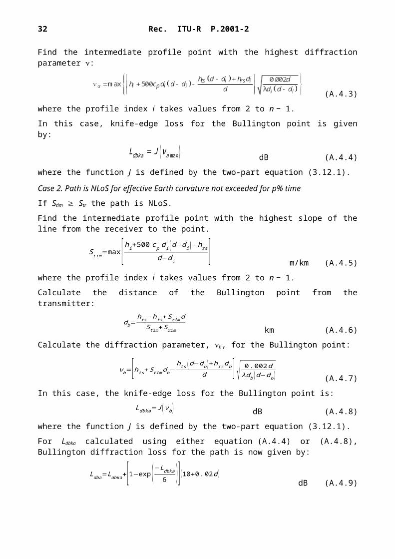
Find the intermediate profile point with the highest diffraction parameter :

24 Rec. ITU-R P.2001-2

(A.4.3)

where the profile index i takes values from 2 to n − 1.

In this case, knife-edge loss for the Bullington point is given by:

Ldbka = J (νa max )                 dB (A.4.4)

where the function J is defined by the two-part equation (3.12.1).

Case 2. Path is NLoS for effective Earth curvature not exceeded for p% time

If Stim  Str the path is NLoS.

Find the intermediate profile point with the highest slope of the line from the receiver to the point.

Srim=max [ hi+500 c p d i (d−di )−hrs

d−d i ]                m/km (A.4.5)

where the profile index i takes values from 2 to n − 1.

Calculate the distance of the Bullington point from the transmitter:

db=hrs−h ts+Srim d

S tim+Srim                 km (A.4.6)

Calculate the diffraction parameter, b, for the Bullington point:

νb=[hts+S timdb−hts (d−db )+hrs db

d ] √ 0. 002 dλdb (d−db ) (A.4.7)

In this case, the knife-edge loss for the Bullington point is:

Ldbka=J (νb )                 dB (A.4.8)

where the function J is defined by the two-part equation (3.12.1).

For Ldbka calculated using either equation (A.4.4) or (A.4.8), Bullington diffraction loss for the path is now given by:

Ldba=Ldbka+[1−exp (−Ldbka

6 )] (10+0 .02d )                dB (A.4.9)

A.5 Bullington diffraction loss for a notional smooth profile

This section calculates the Bullington diffraction loss for a path profile having intermediate points at the same distances as in the actual profile, but with all terrain heights set to zero. The transmitter and receiver heights above this profile are htep and hrep respectively.

The resulting diffraction loss, Ldbs, is calculated as follows.

In the following equations slopes are calculated in m/km relative to the baseline joining sea level at the transmitter to sea level at the receiver.

Find the intermediate profile point with the highest slope of the line from the transmitter to the point relative to the straight line joining sea levels at the terminals.

Rec. ITU-R P.2001-2 25

Stim=max [ 500 (d−d i )ap

−htep

d i ]                 m/km (A.5.1)

where the profile index i takes values from 2 to n − 1.

Calculate the slope of the line from transmitter to receiver assuming a LoS path:

Str=hrep−htep

d                 m/km (A.5.2)

Two cases must now be considered.

Case 1. Path is LoS for effective Earth radius exceeded for p% time

If Stim < Str the path is LoS.

Find the intermediate profile point with the highest diffraction parameter :

(A.5.3)

where the profile index i takes values from 2 to n − 1.

Bullington diffraction loss for the notional smooth terrain profile is given by:

Ldbks=J (νs max )                 dB (A.5.4)

where the function J() is defined by the two-part equation (3.12.1).

Case 2. Path is NLoS for effective Earth radius exceeded for p% time

If Stim  Str the path is NLoS.

Find the intermediate profile point with the highest slope of the line from the receiver to the point.

Srim=max [500 d i

a p−

hrep

d−d i ]                m/km (A.5.5)

where the profile index i takes values from 2 to n − 1.

Calculate the distance of the Bullington point from the transmitter:

db=hrep−htep+Srim d

S tim+Srim                 km (A.5.6)

Calculate the diffraction parameter, b, for the Bullington point:

(A.5.7)

In this case, the knife-edge loss for the Bullington point with a smooth profile is now given by:

Ldbks=J (νb)                 dB (A.5.8)

where the function J() is defined by the two-part equation (3.12.1).

Bullington diffraction loss for the smooth path is now given by:

Ldbs=Ldbks+[1−exp(−Ldbks

6 ) ](10+0. 02 d )                dB (A.5.9)

26 Rec. ITU-R P.2001-2

Attachment B

Clear-air enhancements and fading

B.1 Introduction

This Attachment gives the calculation method for clear-air enhancements and fading. Section B.2 calculates the climate-related, path-dependent, quantity Q0ca which is required by the function Qcaf(A) defined in § B.4. Qcaf(A) may be called many times for the same path. Qcaf(A) gives the percentage of the non-rain time for which a fade level of A exceeds the median signal level during non-rain conditions. Qcaf(A) is used for surface paths. Section B.5 defines the function Qcaftropo(A) that is used for troposcatter paths.

B.2 Characterize multi-path activity

The first part of the multi-path fading calculation characterizes the level of multi-path activity for a given path. It is a preliminary calculation which needs to be completed once for a given path and frequency.

A factor representing the statistics of radio-refractivity lapse rate:

K=10−(4 .6+0.0027 Nd 65 m1 ) (B.2.1)

The parameter Nd65m1 is a parameter characterizing the level of multipath activity for the mid-point of the path. It appears in Table 3.1 and is obtained as described in § 3.4.2.

The notional zero-fade worst-month percentage time characteristic of the deep-fade part of the distribution is calculated as follows. The method depends on whether the path is LoS or NLoS for median time, as determined in § 3.7.

For LoS path:

Calculate the notional zero-fade annual percentage time, Q0ca, using the procedure given in § B.3 with the following inputs:

dca=d                 km (B.2.2a)

ε ca=ε p                 mrad (B.2.2b)

hca=hlo                 m (B.2.2c)

where d, p and hlo appear in Table 3.1 and are calculated in §§ 3.2 and 3.3.

For NLoS path:

In the NLoS case, the notional zero-fade time is evaluated from each antenna to its radio horizon, and the larger of the two results is selected, as follows.

Calculate the notional zero-fade annual percentage time at the transmitter end, Q0cat, using the procedure given in § B.3 with the following inputs:

dca=d lt                 km (B.2.3a)

Rec. ITU-R P.2001-2 27

ε ca=|θt|                mrad (B.2.3b)

hca=min (hts , hi ) with i=ilt    m (B.2.3c)

where dlt, θt, hts and ilt appear in Table 3.1.

Calculate the notional zero-fade annual percentage time at the receiver end, Q0car, using the procedure given in § B.3 with the following inputs

dca=d lr                 km (B.2.4a)

ε ca=|θr|                mrad (B.2.4b)

hca=min (hrs , hi ) with i=ilr    m (B.2.4c)

where dlr, θr, hrs and ilr appear in Table 3.1 and are calculated in §§ 3.3 and 3.7.

The notional zero-fade annual percentage time for the whole path is now given by the larger of the times associated with the transmitter and receiver:

Q0 ca=max(Q0 cat , Q0 car )                 % (B.2.5)

B.3 Calculation of the notional zero-fade annual percentage time

This section calculates the notional zero-fade annual percentage time, Q0ca. The calculation in § B.2 is needed either once or twice depending upon the path type. It requires three input values, dca, εca

and hca, which are specified each time this section is invoked.

Calculate the notional zero-fade worst-month percentage time:

qw=Kd ca3 . 1 (1+ε ca )−1 .29 f 0. 8 10

−0 . 00089 hca                % (B.3.1)

where K is calculated in § B.2 and f appears in Table 3.1.

Calculate the logarithmic climatic conversion factor:

  |mn| ≤ 45 (B.3.2a)

  otherwise (B.3.2b)

where mn is the path mid-point latitude and appears in Table 3.1.

If Cg > 10.8, set Cg = 10.8.

Calculate the notional zero-fade annual percentage time:

Q0 ca=10−0. 1C

gqw                % (B.3.3)

B.4 Percentage time a given clear-air fade level is exceeded on a surface path

This section defines a function Qcaf(A) which gives the percentage of the non-rain time a given fade in dB below the median signal level is exceeded. The method is applicable to both fades (A > 0, when q < 50%) and enhancements (A < 0, when q > 50%) and will return 50% for a median signal

28 Rec. ITU-R P.2001-2

level (A = 0). The calculation is required, possibly several times, during the method for combined clear-air and precipitation fading on a surface path given in § 4.1

The evaluation of Qcaf(A) requires Q0ca as calculated in § B.2 above. For a given path and frequency, Q0ca needs to be calculated only once. Function Qcaf(A) can then be used as often as required in § 4.1.

When A ≥ 0, Qcaf(A) is given by:

Qcaf ( A )=100 {1−exp [−10−0 .05qa A

ln (2)] }                % (B.4.1)

where:

qa=2+(1+0 .3⋅10−0 .05 A ) (10−0 .016⋅A ) [qt+4 . 3(10−0. 05 A+ A800 )] (B.4.1a)

q t=3 .576−1 .955⋅log (Q0 ca ) (B.4.1b)

When A < 0, Qcaf(A) is given by:

  Qcaf ( A )=100exp [−100. 05qe A

ln (2)]        % (B.4.2)

qe=8+ (1+0 .3⋅100 .05 A ) (100.035 A ) [qs+12(100 . 05 A− A800 )] (B.4.2a)

qs=−4 .05−2 .35 log (Q0ca ) (B.4.2b)

B.5 Percentage time a given clear-air fade level is exceeded on a troposcatter path

This section defines a function Qcaftropo(A) which gives the percentage of the non-rain time a given fade in dB below the median signal level is exceeded. The calculation is required, possibly several times, during the method for combined clear-air and precipitation fading on a troposcatter path given in § 4.3.

In WRPM it is assumed that clear-air enhancements and fading are absent on the slant paths between the terminals and the troposcatter common volume. The fade level distribution is therefore a step function:

Qcaftropo( A )=100                % A < 0 (B.5.1a)

Qcaftropo( A )=0                 % otherwise (B.5.1b)

Q0ca does not need to be calculated for troposcatter paths.

Rec. ITU-R P.2001-2 29

Attachment C

Precipitation fading

C.1 Introduction

An iterative procedure is used to combine precipitation and multipath fading for a surface path as described in § 4.1 and for precipitation fading on the two terminal-to-common-volume path segments as described in § 4.3. Thus the calculations described in this Attachment are used for three different paths, each with the climatic parameters obtained for the centre of each path.

The preliminary steps in § C.2 are required before the iterative procedure is used for each of the three paths.

Section C.3 defines function Qrain(A) required by the iteration function Aiter(q) described in Attachment I according to mechanisms as defined in the appropriate subsection of § 4.

C.2 Preliminary calculations

The preliminary calculations require the following inputs:− The longitude and latitude for obtaining rain climatic parameters are denoted here as n and

e. − The heights of the ends of the path for a precipitation calculation are denoted here as hrainlo

and hrainhi, masl.− The length of the path for rain calculations, drain, km.

The values to use for these five input parameters are given where this section is invoked in §§ 4.1 and 4.3.

Obtain Pr6, MT and rain for n and e from the data files, “Esarain_Pr6_v5.txt”, “Esarain_Mt_v5.txt” and “Esarain_Beta_v5.txt”, respectively.

Obtain the mean zero-degree isotherm height rain height h0 in km above sea level for n and e from the data file “h0.txt”.

Calculate mean rain height, hR, in m above sea level:

hR=360+1000 h0               masl (C.2.1)

The variation of rain height throughout an average year is taken into account by the discrete probability distribution in 100 m bins given in Table C.2.1.

Calculate the highest rain height given by:

(C.2.2)

where the constant 2400 is the height difference corresponding to the highest bin of the rain-height distribution in Table C.2.1, that is, for n = 49.

The path must be classified as being either subject to rain or to be a “non-rain” path. This classification is used in § C.3.

If either Pr6 = 0 or hrainlo  hRtop the path is classified as “no-rain”. In this case set Q0ra = 0, Fwvr = 0 and omit the remaining calculations in this subsection. The meaning of these terms is given below in connection with equations (C.2.4) and (C.2.13).

30 Rec. ITU-R P.2001-2

TABLE C.2.1

Probability distribution of rain height

Indexn

Rel. heightH metres

ProbabilityΠ

Indexn

Rel. heightH metres

ProbabilityΠ

1 −2400 0.000555 26 100 0.0495892 −2300 0.000802 27 200 0.0484393 −2200 0.001139 28 300 0.0465834 −2100 0.001594 29 400 0.0441045 −2000 0.002196 30 500 0.0411106 −1900 0.002978 31 600 0.0377247 −1800 0.003976 32 700 0.0340818 −1700 0.005227 33 800 0.0303129 −1600 0.006764 34 900 0.02654210 −1500 0.008617 35 1000 0.02288111 −1400 0.010808 36 1100 0.01941912 −1300 0.013346 37 1200 0.01622513 −1200 0.016225 38 1300 0.01334614 −1100 0.019419 39 1400 0.01080815 −1000 0.022881 40 1500 0.008617

Rec. ITU-R P.2001-2 31

TABLE C.2.1(end)

Indexn

Rel. heightH metres

ProbabilityΠ

Indexn

Rel. heightH metres

ProbabilityΠ

16 −900 0.026542 41 1600 0.00676417 −800 0.030312 42 1700 0.00522718 −700 0.034081 43 1800 0.00397619 −600 0.037724 44 1900 0.00297820 −500 0.041110 45 2000 0.00219621 −400 0.044104 46 2100 0.00159422 −300 0.046583 47 2200 0.00113923 −200 0.048439 48 2300 0.00080224 −100 0.049589 49 2400 0.00055525 0 0.049978

Otherwise the path is classified as “rain”, and the preliminary calculations continue as follows.

Calculate two intermediate parameters given by:

M c= βrain MT (C.2.3a)

M S= (1−βrain ) MT (C.2.3b)

Calculate the percentage of an average year in which rain occurs:

Q0 ra=Pr 6{1−exp(− 0 . 0079 M s

P r6 )}(C.2.4)

Calculate the following three parameters defining the cumulative distribution of rain rate.

a1=1 .09 (C.2.5a)

b1=M c+M s

21797 Q0 ra (C.2.5b)

c1=26 .02b1 (C.2.5c)

Calculate the percentage time approximating to the transition between the straight and curved sections of the rain-rate cumulative distribution when plotted ithmic scale of percentage time:

Qtran=Q0ra exp[ a1 (2 b1−c1)c

12 ](C.2.6)

Use the method given in Recommendation ITU-R P.838 to calculate the rain regression coefficients k and for the frequency, polarization and path inclination. The calculation in Recommendation ITU-R P.838 requires the following values:

f: Frequency in GHz, which has the same symbol in Recommendation ITU-R P.838.

32 Rec. ITU-R P.2001-2

Polarization tilt angle, which in Recommendation ITU-R P.838 has the symbol , given by: = 0 degrees for horizontal linear polarization = 90 degrees for vertical linear polarization.

Path inclination angle, which in Recommendation ITU-R P.838 has the symbol , is given by:

   radians (C.2.7)

In Recommendation ITU-R P.838, trigonometric functions of and are required, and thus the units of these angles must agree with the trigonometric implementation in use. The sign of in Recommendation ITU-R P.838 is immaterial, and thus it is safe to derive its value from p, noting that this is in milliradians.

Note that the method of Recommendation ITU-R P.838 is only valid for frequencies of 1 GHz and above. If the frequency is below 1 GHz, the regression coefficients k1GHz and 1GHz should be calculated for a frequency of 1 GHz and the values of k and obtained as:

k=f k1GHz (C.2.8a)

α=α1GHz (C.2.8b)

Limit the path length for precipitation calculations according to:

dr=min (drain , 300 ) (C.2.9a)

drmin=max (dr , 1 ) (C.2.9b)

Calculate modified regression coefficients given by:

(C.2.10a)

(C.2.10b)

The effect of anomalous attenuation in the melting layer on precipitation fading is assessed by considering each 100 m interval of the distribution in Table C.2.1 in turn. During this process two arrays will be assigned:

Gm: attenuation multiplierPm: probability of a particular case.

When these two arrays have been assigned they will both contain the same number, M, of values. M depends on the geometry of the path relative to the melting layer and has a maximum value of 49. The melting layer is modelled by an attenuation multiplier, , defined by equation (C.4.1). To evaluate the effect of path inclination the melting layer is divided into 12 intervals each 100 m in vertical extent, and a path-averaged multiplier, G, is calculated using the method given in § C.5.

Arrays Gm and Pm are evaluated as follows.

Initialize all Pm to zero.

Initialize G1 = 1. This is not normally necessary, but is advisable to guard against a possible situation where the path is classified as “rain”, but in the following loop b) is executed for every value of n.

Rec. ITU-R P.2001-2 33

Initialize an index m to the first members of arrays G and P: m = 1.

For each line of Table C.2.1, for n from 1 to 49, do the following:a) Calculate rain height given by:

hT = hR + Hn                masl (C.2.11)where Hn is the corresponding relative height entry in Table C.2.1.

b) If hrainlo  hT, repeat from a) for the next value of n. Otherwise continue from c).

c) If hrainhi > hT − 1200 do the following:i) use the method in § C.5 to set Gm to the path-averaged multiplier for this path geometry

relative to the melting layer;ii) set Pm = Πn from Table C.2.1;iii) if n < 49 add 1 to array index m;iv) repeat from a) for the next value of n. Otherwise continue from d).

d) Accumulate Πn from Table C.2.1 into Pm, set Gm = 1, and repeat from a) for the next value of n.

At the end of the above process, set the number of values in arrays Gm and Pm according to:

M = m (C.2.12)

Calculate a factor used to estimate the effect of additional water vapour under rainy conditions given by:

Fwvr=0 .5 [1+ tanh (Rwvr ) ]∑m=1

M

(Gm Pm )(C.2.13)

where:

Rwvr=6 [ log(Q0 ra

q )log( Q0ra

Qtran) ]−3

(C.2.13a)

The values calculated using this § C.2 for a given path or path segment are those to be used in § C.3 for the corresponding iterative procedure. This applies to the classification “rain” or “non-rain”, and in the “rain” case the parameters a, b, c, dr, Q0ra, kmod, mod, the arrays Gm and Pm, and the number of elements in G and P given by M.

C.3 Percentage time a given precipitation fade level is exceeded

This section defines a function Qrain(A) giving the percentage time during which it is raining for which a given attenuation A is exceeded. In order to cover the full distribution negative values of A are included.

When A < 0, Qrain(A) is given by:

Qrain( A )=100    % A < 0 (C.3.1a)

If A ≥ 0 the percentage time for which A is exceeded by precipitation fading depends on whether the path is classified as “non-rain” or “rain”:

34 Rec. ITU-R P.2001-2

Qrain( A )=0    % non-rain (C.3.1b)

Qrain( A )=100 ∑m=1

M

Pm exp[−a Rm (b Rm+1 )(c Rm+1 ) ] % rain (C.3.1c)

where:

   % (C.3.1d)

drlim=max (dr ,0.001 )   km (C.3.1e)

and a, b, c, dr, Q0ra, kmod and mod, and the arrays Gm and Pm, each containing M values, are as calculated in § C.2 for the path or path segment for which the iterative method is in use.

C.4 Melting-layer model

This section defines a function which models the changes in specific attenuation at different heights within the melting layer. It returns an attenuation multiplier, , for a given height relative to the rain height, h in m, given by:

(C.4.1)

where:

δh = h−hT                 (m) (C.4.1a)hT: is the rain height (masl)h: is the height concerned (masl).

The above formulation gives a small discontinuity in at h = −1 200. is clamped to 1 for h < −1 200 to avoid unnecessary calculation and has negligible effect on the final result.

Figure C.4.1 shows how varies with h. For h ≤ −1 200 the precipitation is rain, and  = 1 to give the rain specific attenuation. For −1 200 < h ≤ 0 precipitation consists of ice particles in progressive stages of melting, and varies accordingly, reaching a peak at the level where particles will tend to be larger than raindrops but with fully-melted external surfaces. For 0 < h any precipitation consists of dry ice particles causing negligible attenuation, and  = 0 accordingly.

Rec. ITU-R P.2001-2 35

FIGURE C.4.1Factor (abscissa) plotted against relative height h (ordinate)

Factor represents specific attenuation in the layer divided by the corresponding rain specific attenuation. The variation with height models the changes in size and degree of melting of ice particles.

C.5 Path-averaged multiplier

This section describes a calculation which may be required a number of times for a given path.

For each rain-height hT given by equation (C.2.11), a path-averaged factor G is calculated based on the fractions of the radio path within 100-m slices of the melting layer. G is the weighted average of multiplier given as a function of h by equation (C.4.1) for all slices containing any fraction of the path, and if hlo < hT – 1 200, a value of  = 1 for the part of the path in rain.

Figure C.5.1 shows an example of link path geometry in relation to the height-slices of the melting layer. hlo and hhi (masl) are the heights of the lower and higher antennas, respectively. It should be noted that this diagram is only an example, and does not cover all cases.

FIGURE C.5.1Example of path geometry in relation to melting layer slices

The first step is to calculate the slices in which the two antennas lie. Let slo and shi denote the indices of the slices containing hlo and hhi respectively. These are given by:

slo=1+Floor ( hT−h lo

100 )(C.5.1a)

36 Rec. ITU-R P.2001-2

shi=1+Floor ( hT−hhi

100 )(C.5.1b)

Where the Floor(x) function returns the largest integer that is less than or equal to x.

Note that although slo and shi as calculated by equations (C.5.1a,b) are described as slice indices, they can have values which are less than 1 or greater than 12.

In the following step-by-step description, all conditional tests are defined in terms of slice indices. This ensures that the required comparisons of floating-point heights, including whether the equality is included, are defined by equations (C.5.1a) and (C.5.1b). This is thought to be the simplest way to be confident that all cases are included, but all cases are mutually exclusive.

If slo < 1 the path is wholly above the melting layer. In this case set G = 0, and no further calculation is required.

If shi > 12 the path is wholly at or below the lower edge of the melting layer. In this case set G = 1, and no further calculation is required.

If slo = shi, both antennas are in the same melting-layer slice. In this case G is calculated using:

G=Γ (0 .5 [h lo+hhi]−hT ) (C.5.2)

and no further calculation is required.

Otherwise it is necessary to examine each slice containing any part of the path.

Initialise G for use as an accumulator:G=0 (C.5.3)

Calculate the required range of slice indices using:

s first=max ( shi , 1) (C.5.4a)

slast=min ( slo , 12 ) (C.5.4b)

For all values of slice index s from sfirst to slast do the following:

Start of calculation for each slice index:

For each value of s, exactly one of the following conditions must be true. For the true condition, use the associated equations, (C.5.5a,b), (C.5.6a,b) or (C.5.7a,b), to calculate the height-difference h and the corresponding fraction of the path in the slice Q.

Condition 1: shi < s and s < slo

In this case the slice is fully-traversed by a section of the path:

δh=100 (0 . 5−s ) (C.5.5a)

Q=100hhi−hlo (C.5.5b)

Condition 2: s = slo

In this case the slice contains the lower antenna, at hlo masl:

(C.5.6a)

Rec. ITU-R P.2001-2 37

Q=hT−100 (s−1 )−hlo

hhi−hlo (C.5.6b)

Condition 3: s = shi

In this case the slice contains the higher antenna, at hhi masl:

δh=0 .5 (hhi−hT−100 s) (C.5.7a)

Q=hhi−(hT−100 s)

hhi−hlo (C.5.7b)

Note that all δh values from equations (C.5.5a) to (C.5.7a) should be negative.

For h calculated under one of the preceding three conditions, calculate the corresponding multiplier:

Γ slice=Γ (δh ) (C.5.8)

where as a function of h is defined by equation (C.4.1).

Accumulate the multiplier for this slice:

G = G + Q⋅Γslice (C.5.9)

End of calculation for each slice index:

Having completed the above calculations for each slice index, if the lower antenna is below the melting layer, a further contribution must be made to Gsum. This calculation is as follows:

If slo > 12

The fraction of the path below the layer is given by:

Q=hT−1 200−h lo

hhi−hlo (C.5.10)

Since the multiplier is 1.0 below the layer, G should be increased according to:G=G+Q (C.5.11)

G now has the required value of the path-averaged factor.

Attachment D

Anomalous/layer-reflection model

The basic transmission loss associated with anomalous propagation is calculated as described in the following sections.

D.1 Characterize the radio-climatic zones dominating the pathCalculate two distances giving the longest continuous sections of the path passing through the following radio-climatic zones:

dtm : longest continuous land (inland or coastal) section of the path (km);

38 Rec. ITU-R P.2001-2

dlm : longest continuous inland section of the path (km).Table D.1 describes the radio-climatic zones needed for the above classification.

TABLE D.1

Radio-climatic zones

Zone type Code Definition

Coastal land A1 Coastal land and shore areas, i.e. land adjacent to the sea up to an altitude of 100 m relative to mean sea or water level, but limited to a distance of 50 km from the nearest sea area. Where precise 100 m data are not available an approximate value, i.e. 300 ft, may be used

Inland A2 All land, other than coastal and shore areas defined as “coastal land” aboveSea B Seas, oceans and other large bodies of water (i.e. covering a circle of at least

100 km in diameter)

Large bodies of inland water

A “large” body of inland water, to be considered as lying in Zone B, is defined as one having an area of at least 7 800 km2, but excluding the area of rivers. Islands within such bodies of water are to be included as water within the calculation of this area if they have elevations lower than 100 m above the mean water level for more than 90% of their area. Islands that do not meet these criteria should be classified as land for the purposes of the water area calculation.

Large inland lake or wet-land areas

Large inland areas of greater than 7 800 km2 which contain many small lakes or a river network should be declared as “coastal” Zone A1 by administrations if the area comprises more than 50% water, and more than 90% of the land is less than 100 m above the mean water level.

Climatic regions pertaining to Zone A1, large inland bodies of water and large inland lake and wetland regions, are difficult to determine unambiguously. Therefore administrations are invited to register with the ITU Radiocommunication Bureau (BR) those regions within their territorial boundaries that they wish identified as belonging to one of these categories. In the absence of registered information to the contrary, all land areas will be considered to pertain to climate Zone A2.

For maximum consistency of results between administrations it is recommended that the calculations of this procedure be based on the ITU Digitized World Map (IDWM) which is available from the BR for mainframe or personal computer environments.

If climatic zone codes are inserted into zi as described in § 2.1, dtm and dlm should be calculated on the assumption that when adjacent values of zi differ, the change occurs half-way between the corresponding profile points.

D.2 Point incidence of ducting

Calculate a parameter depending on the longest inland section of the path:

τ =1−exp(−0 .000412 dlm2 . 41) (D.2.1)

Calculate parameter μ1 characterizing the degree to which the path is over land, given by:

Rec. ITU-R P.2001-2 39

μ1 = [10– dtm

16 – 6.6 τ +10– (2. 48 + 1 .77 τ )]0 .2

(D.2.2)

where the value of μ1 shall be limited to μ1  1.

Calculate parameter μ4, given by:

μ4 = {10(−0 .935 + 0.0176 | ϕmn | ) log μ1 for | ϕmn | ≤ 70 °

100 .3 log μ1 for | ϕmn | > 70 ° (D.2.3)

The point incidence of anomalous propagation, β0 (%), for the path centre location is now given by:

β0 = {10−0.015 | ϕmn | + 1. 67 μ1 μ4 % for | ϕmn | ≤ 70 °4 . 17 μ1 μ4 % for | ϕmn | > 70 ° (D.2.4)

D.3 Site-shielding losses with respect to the anomalous propagation mechanism

Corrections to transmitter and receiver horizon elevation angles:

gtr= 0 .1d lt (D.3.1a)

grr= 0 .1 d lr (D.3.1b)

The losses between the antennas and the anomalous propagation mechanism associated with site-shielding are calculated as follows.

Modified transmitter and receiver horizon elevation angles:

θst=θt−g tr                    mrad (D.3.2a)

θsr=θr−grr                 mrad (D.3.2b)

Transmitter and receiver site-shielding losses with respect to the duct:

dB st > 0 (D.3.3a)

A st=0                 dB otherwise (D.3.3b)

dB sr > 0 (D.3.4a)

A sr=0                 dB otherwise (D.3.4b)

D.4 Over-sea surface duct coupling corrections

Obtain the distance from each terminal to the sea in the direction of the other terminal:

dct = coast distance from transmitter                km (D.4.1a)

dcr = coast distance from receiver                km (D.4.1b)

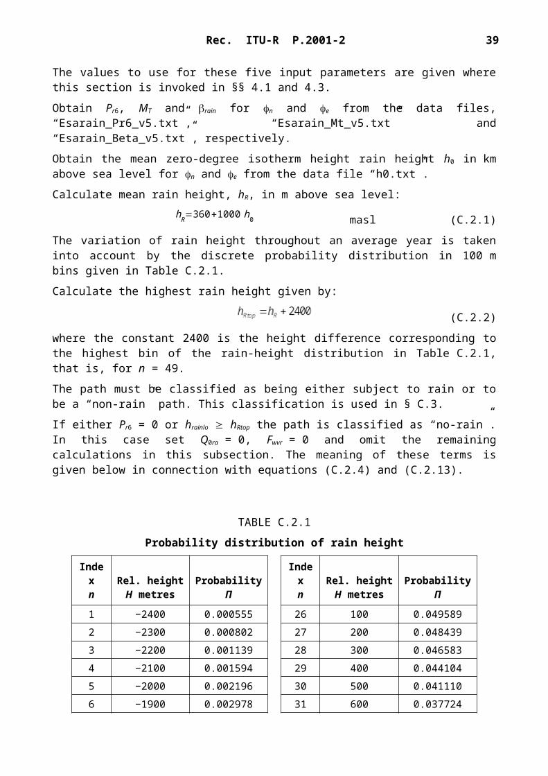
40 Rec. ITU-R P.2001-2

As for dtm and dlm in § D.1 above, it is preferable to obtain the distances over land to the first coast from the IDWM. If climatic zone codes are inserted into zi as described in § 2.1, dct and dcr should be calculated on the assumption that when adjacent values of zi differ, the change occurs half-way between the corresponding profile points.

The over-sea surface duct coupling corrections for the transmitter and receiver, Act and Acr

respectively, are both zero except for the following combinations of conditions:

   Act=−3exp (−0 .25 dct2 ) [1+ tanh {0. 07 (50−hts )}]              dB

if ( 0.75) and (dct ≤ dlt) and (dct ≤ 5 km) (D.4.2a)

Act=0                 dB otherwise (D.4.2b)

Acr=−3exp (−0 . 25 dcr2 ) [1+ tanh {0. 07 (50−hrs )} ]                 dB

if ( 0.75) and (dcr ≤ dlr) and (dcr ≤ 5 km) (D.4.3a)

Acr=0                 dB otherwise (D.4.3b)

where is the fraction of the path over sea as given in Table 3.1.

D.5 Total coupling loss to the anomalous propagation mechanism

The total coupling losses between the antennas and the anomalous propagation mechanism can now be calculated as:

Aac=102 . 45+20 log [ f (d lt+d lr )]+Alf +A st+A sr+Act+Acr                 dB (D.5.1)

Alf is an empirical correction to account for the increasing attenuation with wavelength in ducted propagation:

Alf=(45 .375−137 . 0 f +92 .5 f 2) ω dB if f < 0.5 GHz (D.5.2a)

Alf=0                dB otherwise (D.5.2b)

where is the fraction of the path over sea as given in Table 3.1.

D.6 Angular-distance dependent loss

Specific angular attenuation within the anomalous propagation mechanism:

                dB/mrad (D.6.1)

Adjusted transmitter and receiver horizon elevation angles:

                mrad (D.6.2a)

                mrad (D.6.2b)

Adjusted total path angular-distance:

                mrad (D.6.3)

Angular-distance dependent loss:

Rec. ITU-R P.2001-2 41

                dB (D.6.4)

D.7 Distance and time-dependent loss

The loss in the anomalous propagation mechanism dependent on both great-circle distance and percentage time are calculated by first evaluating the following.

Distance adjusted for terrain roughness factor:

dar=min (d−d lt−dlr , 40 )                 km (D.7.1)

Terrain roughness factor:

hm > 10 m (D.7.2a)

μ3=1otherwise (D.7.2b)

A term required for the path geometry correction

(D.7.3)

If α < −3.4, set α = −3.4

Path-geometry factor:

μ2=[ 500 d2

ae (√htea+√hrea )2 ]

α

(D.7.4)

If 2 > 1, set 2 = 1

Time percentage associated with anomalous propagation adjusted for general location and specific properties of the path:

βduct=β0 μ2 μ3                 % (D.7.5)

An exponent required for the time-dependent loss:

Γ=1 . 076exp {−10−6 d1. 13 [9 .51−4 .8 log βduct+0 .198 (log βduct )2 ]}

(2.0058− log βduct )1. 012

(D.7.6)The time-dependent loss:

Aat=−12+(1 .2+0 . 0037 d ) log ( pβduct )+12 ( p

βduct )Γ+50

q          dB (D.7.7)

D.8 Basic transmission loss associated with ducting

Basic transmission loss associated with anomalous propagation is given by:

Lba=Aac+Aad+Aat    dB (D.8.1)

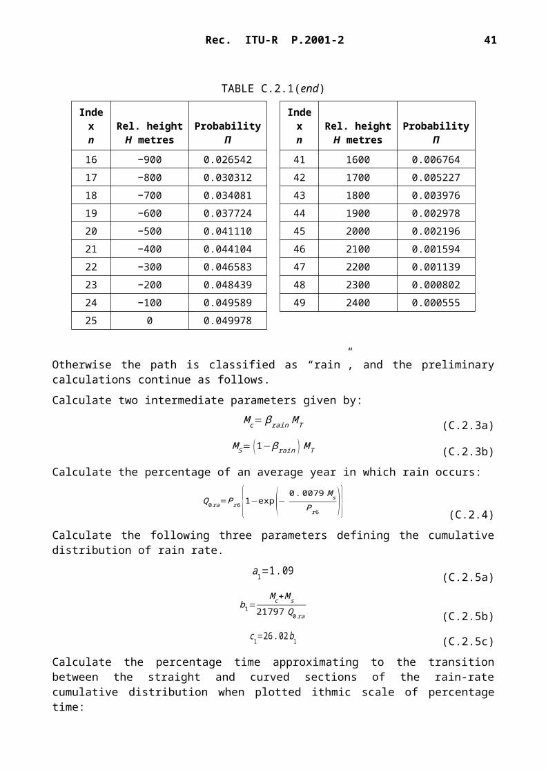
42 Rec. ITU-R P.2001-2

Attachment E

Troposcatter

E.1 Introduction

The following sections give the method for calculating troposcatter basic transmission loss Lbs not exceeded for a given percentage of an average year. The method is based on selecting an appropriate climatic zone.

E.2 Climatic classification

This sub-model is based on the use of climate zones as shown in Fig. E.1. The zone corresponding to the latitude and longitude of the troposcatter common volume, cvn and cve, should be read from the file “TropoClim.txt”. This file contains integers in the range 0 to 6. Integers 1 to 6 correspond to the climate zones shown in Fig. E.1. Integer 0 represents a sea location for which a special procedure is required.

FIGURE E.1Climatic zones

In case the troposcatter common volume lies over the sea, the climates at both the transmitter and receiver locations should be determined. If both terminals have a climate zone corresponding to a land point, the climate zone of the path is given by the smaller value of the transmitter and receiver climate zones. If only one terminal has a climate zone corresponding to a land point, then that climate zone defines the climate zone of the path. If neither terminal has a climate zone corresponding to a land point, the path is assigned a “sea path” climate zone in Table E.1.

Obtain the meteorological and atmospheric structure parameters M and , respectively, from Table E.1 for the climate zone in question.

The last row of Table E.1 gives the number of the equation used to calculate Y90 in § E.3 below.

Rec. ITU-R P.2001-2 43

TABLE E.1

Meteorological and atmospheric structure parameters

Climate zone 1 2 3 4 5 6 Sea path

M (dB) 129.60 119.73 109.30 128.50 119.73 123.20 116.00 (km−1) 30.33 20.27 10.32 30.27 20.27 30.27 20.27

Y90 eq (E.8) (E.6) (E.9) (E.10) (E.6) (E.6) (E.7)

E.3 Calculation of troposcatter basic transmission loss

The scatter angle is given by:

                mrad (E.1)

where the three “thetas” on the right-hand side all appear in Table 3.1.

The loss term dependent on the common-volume height is given by:

LN=20 log (5+γH )+4 .34 γ htrop                 dB (E.2)

where:

H=0. 25⋅10−3 θ d                 km (E.3)

htrop=0. 125⋅10−6 θ2ae                 km (E.4)

and d and ae appear in Table 3.1.

Calculate the angular distance of the scatter path based on median effective Earth radius, which is used in the following equations:

d s=0. 001 θ ae                 km (E.5)

Calculate Y90 (dB) using one of equations (E.6) to (E.10) as selected from Table E.1:

Y 90=−2.2−[8 .1−0 . 23 min ( f ,4 ) ] exp (−0.137 htrop ) (E.6)

where f appears in Table 3.1.

Y 90=−9 .5−3exp (−0 . 137 htrop ) (E.7)

Y 90=¿ {−8 .2 d s<100 ¿ {1. 006⋅10−8 d s3−2 .569⋅10−5 d s

2+0 .02242 ds−10 . 2100≤ds<1000 ¿ ¿¿¿(E.8)

Y 90=¿ {−10 .845 d s<100 ¿ {−4 .5⋅10−7 d s3+4 . 45⋅10−4 ds

2−0 .122 ds−2 .645 100≤ds<465 ¿ ¿¿¿(E.9)

44 Rec. ITU-R P.2001-2

Y 90=¿ {−11.5 d s<100 ¿ {−8 .519⋅10−8 ds3+7 .444⋅10−5 d s

2−4 .18⋅10−4 ds−12.1 100≤d s<550 ¿¿¿¿(E.10)

Calculate a conversion factor given by:

C=1 .26 {−log [100−p50 ]}

0 .63

p ≥ 50 (E.11a)

C=−1 .26 {− log [ p50 ]}

0. 63

otherwise (E.11b)

The parameter Yp not exceeded for p% time is now given by:

Y p=C Y 90                 dB (E.12)

Limit the value of θ such that θ  10−6.

Calculate the distance and frequency dependent losses using:

Ldist=max [10 log (d )+30 log (θ )+LN , 20 log (d )+0 .573 θ+20 ]                 dB (E.13)

Lfreq=25 log (f )−2. 5 [ log (0 .5 f ) ]2                 dB (E.14)

Calculate the aperture-to-medium coupling loss using:

Lcoup=0 . 07 exp [0 . 055 (Gt+Gr ) ]                 dB (E.15)

The troposcatter basic transmission loss not exceeded for p% time is now given by

Lbs=M+Lfreq+Ldist+ Lcoup−Y p                 dB (E.16)

To avoid under-estimating troposcatter loss for short paths, limit Lbs such that

Lbs≥Lbfs                 dB (E.17)

where free-space basic transmission loss Lbfs appears in Table 3.1.

Attachment F

Attenuation due to gaseous absorption

F.1 Introduction

This Attachment describes methods for calculating the attenuation due to gaseous absorption for different types of radio path. The sections of this Attachment are referenced elsewhere as required.

The calculations require surface water-vapour density sur g/m3 for locations of interest. Values for sur may be obtained from the data file “surfwv_50_fixed.txt”.

Rec. ITU-R P.2001-2 45

Each calculation produces three values of attenuation, due to absorption by: oxygen, water vapour under non-rain conditions, water vapour under rain conditions.

F.2 Gaseous absorption for surface path

This section gives the method for calculating gaseous absorption for a “surface” path.

Obtain surface water-vapour density under non-rain conditions, sur, g/m3, at the mid-point of the path, as given by me and mn in Table 3.1, from the data file “surfwv_50_fixed.txt”.

Set hsur = hmid. The terrain height at the middle of the path, hmid, appears in Table 3.1.

Use equation (F.6.2) to calculate the sea-level specific attenuation due to water vapour under non-rain conditions, w, dB/km.

Use equation (F.5.1) to calculate the surface water-vapour density under rain conditions, surr, g/m−3.

Re-evaluate sur according to sur = surr.

Use equation (F.6.2) to calculate the sea-level specific attenuation due to water vapour under rain conditions, wr, dB/km.

Calculate the height for water-vapour density:

hrho = 0 .5 (hts+hrs)                 masl (F.2.1)

The three attenuations due to gaseous attenuation for the surface path are now given by:

Attenuation due to oxygen:

                dB (F.2.2a)

where o, the sea-level specific attenuation due to oxygen, appears in Table 3.1.

Attenuation due to water-vapour under non-rain conditions:

                dB (F.2.2b)

Attenuation due to water-vapour under rain conditions:

                dB (F.2.2c)

F.3 Gaseous absorption for a troposcatter path

This section gives the method for calculating gaseous absorption for a complete troposcatter path, from transmitter to receiver via the common scattering volume.

Obtain surface water-vapour density under non-rain conditions, sur, g/m3, at the location of the transmitter, as given by te and tn in Table 2.2.1, from the data file “surfwv_50_fixed.txt”.

Use the method in § F.4, with hsur = h1, elev = tpos, dcv = dtcv , to give the gaseous attenuations due to oxygen, and for water vapour under both non-rain and rain conditions, for the transmitter/common-volume path, where h1 is the height of the first profile point in metres above sea level, and tpos and dtcv appear in Table 3.1. Save the values calculated by equations (F.4.3a) to (F.4.3c) according to:

Aotcv=Ao                 dB (F.3.1a)

46 Rec. ITU-R P.2001-2

Awtcv=Aw                 dB (F.3.1b)

Awrtcv=Awr                 dB (F.3.1c)

Obtain surface water-vapour density under non-rain conditions, sur, g/m3, at the location of the receiver, as given by re and rn in Table 2.2.1, from the data file “surfwv_50_fixed.txt”.

Use the method in section F.4, with hsur = hn, elev = rpos, dcv = drcv to give the gaseous attenuations due to oxygen, and for water vapour under both non-rain and rain conditions, for the receiver/common-volume path, where hn is the height of the last profile point in metres above sea level, and rpos, and drcv appear in Table 3.1. Save the values calculated by equations (F.4.3a) to (F.4.3c) according to:

Aorcv=Ao                 dB (F.3.2a)

Awrcv=Aw                 dB (F.3.2b)

Awrrcv=Awr                 dB (F.3.2c)

The gaseous attenuations due to oxygen and for water vapour under both non-rain and rain conditions, for the complete troposcatter path are now given by:

Aos=Aotcv+Aorcv                 dB (F.3.3a)

Aws=Awtcv+Awrcv                 dB (F.3.3b)

Awrs=Awrtcv+Awrrcv                 dB (F.3.3c)

F.4 Gaseous absorption for terminal/common-volume troposcatter path

This section gives the method for calculating gaseous attenuation under non-rain conditions for the path from one terminal to the common volume of a troposcatter path. The inputs are surface water-vapour density under non-rain conditions, sur, g/m3, terrain height hsur masl, elevation angle of path elev mrad, and horizontal distance to the common volume dcv km, as specified on each of the two occasions when this section is used as described in section F.3 above.

The outputs are the attenuations due to oxygen, and due to water vapour under both non-rain and rain conditions, for the terminal/common-volume path, Ao, Aw and Awr, in dB.

Use equation (F.6.2) to calculate the sea-level specific attenuation due to water vapour under non-rain conditions, w, dB/km.

Use equation (F.5.1) to calculate the surface water-vapour density under rain conditions, surr, g/m−3.

Re-evaluate sur according to sur = surr.

Use equation (F.6.2) to calculate the sea-level specific attenuation due to water vapour under rain conditions, wr, dB/km.

Calculate the quantities do and dw for oxygen and water vapour:

do=5

0 .65sin (0 .001 θelev )+0 . 35√sin2 (0 . 001θelev )+0 .00304 (F.4.1a)

dw=2

0 . 65 sin (0 .001 θelev )+0. 35√sin2 (0 . 001θelev )+0 . 00122 (F.4.1b)

Rec. ITU-R P.2001-2 47

Calculate the effective distances deo and dew for oxygen and water vapour:

deo=do(1−e

−dcv

do ) exp(− hsur

5000 )                 km (F.4.2a)

dew=dw(1−e

−dcvdw ) exp (− hsur

2000 )                 km (F.4.2b)

The attenuations due to oxygen, and for water vapour under both non-rain and rain conditions, for the terminal/common-volume path are now given by:

Ao=γ o deo                 km (F.4.3a)

Aw=γ w dew                 km (F.4.3b)

Awr=γ wr dew                 km (F.4.3c)

where o, the sea-level specific attenuation due to oxygen, appears in Table 3.1.

F.5 Water-vapour density in rain

This section gives the method for calculating atmospheric water-vapour density in rain. The two-part equation (F.5.1) is used by the preceding sections.

ρ surr={ρ sur+0.4+0.0003 hsur hsur ≤ 2600m

ρsur+5 exp(−hsur

1800 )otherwise(F.5.1)

F.6 Specific sea-level attenuations

This section gives equations used in the preceding sections. Note that these equations are not valid for frequencies greater than 54 GHz. More general expressions are available in Recommendation ITU-R P.676.

Sea-level specific attenuation due to oxygen:

                dB/km (F.6.1)

Sea-level specific attenuation due to water-vapour in dB/km:

(F.6.2)where:

(F.6.2a)

ρ sea=ρsur exp( hsur

2000 )                g/m3 (F.6.2b)

48 Rec. ITU-R P.2001-2

Attachment G

Sporadic-E propagation

This Attachment describes a method giving sporadic-E basic transmission loss not exceeded for p% time based on maps of foEs exceeded for 0.1%, 1%, 10% and 50% of an average year (FoEs0.1.txt, FoEs01.txt, FoEs10.txt and FoEs50.txt, respectively). It is intended primarily to predict interference on long paths for low and mid-latitudes. The method should not be considered reliable at low or high geomagnetic latitudes, and it need not be calculated for a LoS path. It should be noted that incidents of high signal strength due to this phenomenon exhibit a very strong seasonal dependence.

The calculation includes terminal shielding, which varies according to take-off angle. Thus for all path lengths the calculation is made for both 1 hop and 2 hops. These two results are combined at the end of the procedure.

G.1 Derivation of foEs

For a given p% time, set the percentage-time values used for interpolation or extrapolation, p1 and p2 according to Table G.1.

TABLE G.1

Conditions for setting p1 and p2

p% time p1 p2

p < 1% 0.1% 1%1% ≤ p ≤ 10% 1% 10%

10% < p 10% 50%

For a given location, obtain foEs1 and foEs2 from the maps of foEs exceeded for p1 and p2% time respectively. Calculate foEs exceeded for p% time using:

f oEs= f oEs 1+( f oEs 2− f oEs1 )[ log( pp1 )

log( p2

p1) ]

                MHz (G.1.1)

G.2 1-hop propagation

Obtain foEs in MHz as calculated by equation (G.1.1) for the mid-point of the path.

Calculate the ionospheric loss for one hop:

Γ1 = [40

1 + ( d130 ) + ( d

250 )2 +0. 2 ( d

2600 )2 ] (1000 f

f oEs )2+ exp( d – 1660

280 )(G.2.1)

Calculate the slope path length:

Rec. ITU-R P.2001-2 49

l1=2[ae2+ (ae+hes )2−2 ae (ae+hes )cos ( d2 ae )]

0.5

                km (G.2.2)

where hes is the height of the sporadic-E layer in km, set to 120 km.

Free-space loss can now be calculated for the slope distance:

Lbfs 1=LbfsD (l1) (G.2.3)

where the function LbfsD is defined by equation (3.11.1).

The ray take-off angle above the local horizontal at both terminals for 1 hop is given by:

                rad (G.2.4)

where:

                rad (G.2.4a)

The diffraction angles for the two terminals are given by:

δ1t , 1r=0 .001 θt , r−εr 1                 rad (G.2.5)

The corresponding diffraction parameters are given by:

if δ1t ,1r≥0

(G.2.6a)

otherwise (G.2.6b)

The diffraction losses at the two terminals are then given by:

Lp 1t=J (ν1t )                 dB (G.2.7a)

Lp 1r=J (ν1r )                 dB (G.2.7b)

where the function J is defined by the two-part equation (3.12.1).

Sporadic-E 1-hop basic transmission loss is now given by:

LbEs1=Lbfs 1+Γ1+Lp1 t+ Lp1 r                 dB (G.2.8)

G.3 2-hop propagation

Obtain foEs2h as the lower of the two values calculated by equation (G.1.1) at one-quarter and three-quarters along the path. The latitude and longitude of the one-quarter and three-quarter points can be obtained using the great circle path method of Attachment H by setting dpnt = 0.25 d and dpnt = 0.75 d in equation (H.3.1) respectively.

Calculate the ionospheric loss for two hops:

50 Rec. ITU-R P.2001-2

Γ2 = [40

1 + ( d260 ) + ( d

500 )2 +0. 2 ( d

5200 )2 ] (1000 f

f oEs2 h )2+ exp( d – 3220

560 )(G.3.1)

Calculate the slope path length:

l2=4 [ae2+(ae+hes )2−2ae (ae+hes )cos ( d4 ae )]

0.5

                km (G.3.2)

Free-space loss can now be calculated for the slope distance:

Lbfs 2=LbfsD (l2) (G.3.3)

where the function LbfsD is defined by equation (3.11.1).

The ray take-off angle above the local horizontal at both terminals for 2 hops is given by:

                rad (G.3.4)where:

                rad (G.3.4a)

The diffraction angles for the two terminals are given by:

δ2t , 2 r=0 .001 θt , r−εr 2                 rad (G.3.5)

The corresponding diffraction parameters are given by:

The diffraction losses at the two terminals are then given by:

Lp 2t=J (ν2t )                 dB (G.3.7a)

Lp 2r=J (ν2r )                 dB (G.3.7b)

where the function J is defined by the two-part equation (3.12.1).

Sporadic-E 2-hop basic transmission loss is now given by:

LbEs2=Lbfs 2+Γ 2+Lp 2t+Lp 2r                 dB (G.3.8)

Rec. ITU-R P.2001-2 51

G.4 Basic transmission loss

Basic sporadic-E transmission loss, Lbe (dB) is now given by:

Lbe={ LbEs1 LbEs1<LbEs 2−20 (G . 4 .1a )LbEs2 LbEs2<LbEs1−20 (G . 4 . 1b)

−10 log (10−0 .1 LbEs 1+10−0 . 1 LbEs2) otherwise (G . 4 .1c )

Attachment H

Great-circle path calculations

H.1 Introduction

This Attachment gives guidance on the calculation of intermediate points on the radio path when latitude and longitude coordinates must be used.

The most important application is to find the mid-point of the radio path, which is the location for which most radio-climatic parameters should be obtained. The sporadic-E model of Attachment G also requires the points one-quarter and three-quarters along the path.

The terminal locations are defined in the basic input parameters listed in Table 2.2.1 in the main body of this Recommendation in terms of latitude and longitude. This is because it is expected that radio-climatic parameters will be obtained from global maps which require these coordinates. For short paths, which according to the accuracy required might be defined as less as 100 km. It may be sufficiently accurate and more convenient to convert the terminal locations to Cartesian coordinates, such as within a national grid or one of the UTM grids, calculate intermediate path points using Cartesian geometry, and convert back to latitude and longitude to obtain radio-climatic parameters.

In the following sections, the units of some angles are not stated. They will depend on the units required by the implementation of trigonometric functions, and conversion must be made as required.

H.2 Path length and bearing

The method requires the path length, d, (km), which is available from the profile. It may be a useful check to calculate the path length directly from the terminal coordinates.

Calculate the difference in longitude between the terminals, given by:

Δlon=φre−φte                 degrees (H.2.1)

Calculate the quantity r:

r=sin (φ tn)sin (φrn)+cos (φ tn)cos (φrn )cos ( Δlon ) (H.2.2)

Calculate the path length as the angle subtended at the centre of average-radius Earth:

φd=arccos ( r ) (H.2.3)

Calculate the great-circle path length:

52 Rec. ITU-R P.2001-2

d gc=φdrad Re                 km (H.2.4)

where drad is d in radians, and Re is given in Table 2.3.1.

As commented in § H.1 above, the value of dgc can be compared to d, as given in Table 2.2.1 and obtained in § 3.2, as a consistency test.

Calculate the quantities x1 and y1:

x1=sin (φrn)−r sin (φtn) (H.2.5a)

y1=cos (φtn )cos (φrn)sin (Δlon) (H.2.5b)

Calculate the bearing of the great-circle path from the transmitter towards the receiver, Bt2r, as the angle between due north at the transmitter eastwards (clockwise) to the direction of the path. For numerical reasons it is necessary to trap very small absolute values of the arguments of the inverse trigonometric function:

(H.2.6)

where the function “arctan2” calculates the angle between the line joining the Cartesian origin to a point at (x,y) and the X-axis, giving Bt2r in the correct quadrant, and allowing either x or y, but not both, to be zero.

If the function “arctan2” is not available from a library it can be implemented by inspecting x and y and using the normal inverse tangent function for an angle not exceeding 45 degrees, which can always be found.

H.3 Calculation of intermediate path point

The following calculation gives the latitude and longitude of any point along the path from transmitter to receiver. The value of the distance from the transmitter to the intermediate point, dpnt

(in km), is defined at the place in the document where this section is used.

Calculate the distance to the point as the angle subtended at the centre of average-radius Earth:

φ pnt=d pnt /Re                 rad (H.3.1)

Note that equation (H.3.1) gives pnt in radians.

Calculate the quantity s:

s=sin (φtn )cos (φpnt )+cos (φtn)sin (φpnt )cos (Bt 2r ) (H.3.2)

The latitude of the intermediate point is now given by:

φ pntn=arcsin ( s ) (H.3.3)Calculate the quantities x2 and y2:

x2=cos (φ pnt )−s sin (φ tn) (H.3.4a)

y2=cos (φtn) sin(φpnt )sin (Bt 2r ) (H.3.4b)

Calculate the longitude of the intermediate point, pnte. For numerical reasons it is necessary to trap very small absolute values of the arguments of the inverse trigonometric function:

Rec. ITU-R P.2001-2 53

φ pnte=¿ {Bt 2 r if|x2|<10−9 and|y2|<10−9 ¿ ¿¿¿(H3.5)

If necessary, adjust pnte to lie in the correct 360º range. Most implementations of the arctan2 function will return a value in the range −180º to 180º as required.

Attachment I

Iterative procedure to invert a cumulative distribution function

I.1 Introduction

This Attachment defines an iterative procedure that can be used to calculate the attenuation level A of a propagation mechanism for a given value of q% time for which A is exceeded. The function A(q) is an inverse cumulative distribution function. The iterative procedure is necessary when the propagation model is formulated to calculate the time percentage, q, for which a given level of attenuation A is exceeded. The function Q(A) is a cumulative distribution function.

The WRPM model fundamentally calculates A for a given value of q or p. However, the clear-air and precipitation sub-models are formulated to calculate q for a given value of A. Inversion of the cumulative distribution function is therefore required for these sub-models, and in particular for the combining of these two sub-models.

Note that although the procedure defined in this Attachment is formulated in terms of fades, A, it will handle both fades (A > 0) and enhancements (A < 0).

I.2 Iteration method

This section defines a function Aiter(q) which gives the attenuation due to the selected propagation mechanisms exceeded for q% time. In several places the procedure calls a function Qiter(A). Qiter(A) is the cumulative distribution function of the propagation model for which Aiter(q) is required. Qiter(A) is defined in the main text at the point where the iterative procedure of this Attachment is required.

Qiter(A) has a negative slope; therefore, it should be noted that whilst Ahigh is greater than Alow, qhigh is smaller than qlow.

The iteration proceeds in two stages. Firstly a search range of attenuation levels is found which is known to include the required percentage fade time. Secondly a binary search is used to refine the search until the resulting percentage time is within the given tolerance of the target percentage fade time.

Stage 1: setting the search range

The initial value of trial attenuation, Ainit, can be set to any non-zero positive value. There may be efficiency reasons to calculate Ainit on some objective basis. However, simply setting Ainit to 10 dB has been found to give reasonable efficiency in the iteration process.

54 Rec. ITU-R P.2001-2

Set the initial values of the high and low search limits for attenuation and the attenuation step size, given by:

Ahigh=A init

2                 dB (I.2.1)

Alow=−A init

2                 dB (I.2.2)

Astep=A init                 dB (I.2.3)

Initialize the percentage times attenuations Ahigh and Alow are exceeded:

qhigh=Qiter ( Ahigh )                 dB (I.2.4a)

q low=Qiter ( Alow )                 dB (I.2.4b)

Stage 1: initial search range iteration:

If q < qhigh, proceed as follows:Re-evaluate Alow = Ahigh;Re-evaluate qlow = qhigh;Re-evaluate Astep = 2 × Astep;Re-evaluate Ahigh = Ahigh + Astep;Re-evaluate qhigh using equation (I.2.4a);Loop back to the start of search range iteration and repeat from there.

If q > qlow, proceed as follows:Re-evaluate Ahigh = Alow;Re-evaluate qhigh = qlow;Re-evaluate Astep = 2 × Astep;Re-evaluate Alow = Alow − Astep;Re-evaluate qlow using equation (I.2.4b);Loop back to the start of initial search range iteration and repeat from there.

Otherwise, that is if q ≥ qhigh and q ≤ qlow, proceed to stage 2. The initial search range loop will normally require only a few iterations. To ensure numerical stability, the loop should be terminated after 10 iterations irrespective of the values of qlow and qhigh, and the calculation continued from stage 2.

Stage 2: binary search

Evaluate Atry:

Atry=0 . 5 ( A low+Ahigh )                 dB (I.2.5)Start of binary search iteration:

Calculate the percentage time attenuation Atry is exceeded:

q try=Qiter ( Atry )                 % (I.2.6)If qtry < q re-evaluate Ahigh = Atry.Otherwise, re-evaluate Alow = Atry.

Rec. ITU-R P.2001-2 55

Re-evaluate Atry using equation (I.2.5).Loop back to the start of binary search iteration and repeat from there. The number of iterations of the binary search loop, niter, determines the absolute accuracy of the calculated function Aiter(q). To achieve an accuracy better than Aacc set niter to the smallest integer value

greater than or equal to 3 .32 log ( A step /Aacc) . Aacc = 0.01dB should be adequate. Once niter

iterations have been completed, continue below.

The attenuation exceeded for q% time is approximated by:

q try=Qiter ( Atry )                 % (I.2.7)

Attachment J

Structure of the wide-range propagation model

J.1 Introduction

This Attachment describes the structure of the overall wide-range propagation model and explains how the methods used to combine the sub-models reflect the underlying correlation properties of the sub-models.

The model is based on the notion of combining seven sub-models representing seven separate propagation mechanisms. These are diffraction, ducting, troposcatter, sporadic-E, gaseous absorption, precipitation attenuation and multipath/focusing. The first four are mechanisms that provide end-to-end paths from transmitter to receiver. The radio waves for each of these in principle follow a different path through the atmosphere, and the four paths act “in parallel”. The last three do not by themselves provide signal paths between transmitter and receiver. Rather they are additive attenuation mechanisms that produce additional loss on the four end-to-end paths.

Combining the seven models is not trivial because they are time-dependent, statistical, models. The correlation properties of the models are central to the method. The model correlations reflect the correlations of the underlying meteorological mechanisms that cause the time variability. A recent re-examination of long-term, global meteorological data was used to define the correlations between the various sub-models. Simplifications had to be made in order to develop a model that was relatively simple to implement – in general numerical methods would be required to represent the full statistical properties of the propagation mechanisms.

J.2 Combining the sub-models

Figure J.2.1 shows the structure of the overall model. The double outlining of the boxes and the double-width lines in the diagram represent the fact that what flows through the diagram is not a signal or power, but a whole statistical distribution of power/loss. Specifically it is the inverse cumulative distribution function (ICDF) of the models. This specifies the distribution of basic transmission loss values L as a function of time percentage p. The model combiners are represented by the circles. The letter in a combiner specifies the correlation property of the combiner: “C” means fully correlated, “E” means mutually exclusive and “U” means uncorrelated. The “S” combiners are scalar combiners where one of the quantities being combined is a simple number (typically a median value) rather than a full distribution.

56 Rec. ITU-R P.2001-2

The details of how the sub-model predictions are combined are given explicitly in §§ 4 and 5. But for information, the basic formulae used for combining two distributions, assuming the four types of correlation properties used, are given here.

In the following equations L represents a basic transmission loss of one of the four parallel end-to-end propagation models. A represents the attenuation relative to free space produced by one of the additive models. We write L(p) or A(p) for the value of an ICDF at a time percentage p. Suffixes in1, in2 and out are used in the obvious way for ICDFs and scal for a scalar input.

Combining two ICDFs that are fully correlated (a “C” combiner) is simply a matter of adding powers or losses at time percentage p. The way this is done depends on whether the models to be combined are expressed in terms of two basic transmission losses, or a basic transmission loss and an attenuation relative to free space:

Lout ( p )=−10 log (10−0 .1 Lin 1( p )+10−0 . 1 Lin 2( p ))                 dB (J.2.1a)

Lout ( p )=Lin 1( p)+A in2( p )                dB (J.2.1b)

Combining an ICDF and a constant value (an “S” combiner), for example a single median value of attenuation, is also simple. The output ICDF is just the input ICDF “shifted” along the power/loss axis by the value of the input scalar quantity:

Lout ( p )=Lin 1( p)+A in2                 dB (J.2.2)

Note that “C” and “S” combinations can be done “point by point”, that is the output value at p% of the time only depends on the p% values of the input models, and does not require the full distributions.

Combining mutually exclusive mechanisms (an “E” combiner) is more difficult to implement computationally, but is conceptually simple. The time percentages of the two input ICDFs are added at each value of loss:

pout (A )=p in1( A )+ pin 2(A )                dB (J.2.3)

This requires an iterative procedure that uses the full distributions of the input quantities. This method is used for combining the clear-air and precipitation mechanisms.

Surprisingly perhaps, combining two ICDFs that are uncorrelated (a “U” combiner) is the most difficult. Indeed numerical techniques, such as Monte-Carlo, are required to do this properly. When WRPM is used for Monte-Carlo simulations, the structure of the WRPM model allows the statistics to be correctly modelled in a fairly straightforward way. This is described in § 5.3.

However, it is recognized that WRPM will often be used in circumstances that do not justify the computational complexity of a Monte-Carlo simulation. In that case a simple ansatz is applied to allow the full-model basic transmission loss to be calculated at a single value of time percentage. The principle is to select the strongest signal, or equivalently the lowest value of basic transmission loss, from the two (or more) signal paths at each time percentage p. A “blend” function can be used to eliminate the slope discontinuities that a simple picking of the minimum value would entail. The following method is used in § 5.2:

Lout ( p )=−5 log (10−0 . 2 Lin1( p )+10−0 . 2 Lin 2( p ))                 dB (J.2.4)

Although this looks very similar to the method of equation (J.2.1a) and has the advantage that the combination can be done on a “point by point” basis, “U” and “C” combiners are statistically very different. Maintaining the logical separation here makes it easier for an implementer of the model to

Rec. ITU-R P.2001-2 57

apply numerical methods to give a more statistically correct result than the simple analytical approach of equation (J.2.4).

Note that equations (J.2.1a) and (J.2.4) could encounter a numerical problem if the sub-model basic transmission losses are very large. Numerical limitations could cause the argument of the log function to be zero. This is avoided by using the mathematically equivalent formulation of these equations given in § 5. This factors out the basic transmission loss of the dominant sub-model and adds to it a correction that takes account of the other sub-models.

FIGURE J.2.1Sub-model combination diagram