As the number and complexity of power system planning models grows, understanding the impact ofmodeling choices on accuracy and computational requirements becomes increasingly important. Thisstudy examines empirically various temporal and spatial tradeoffs using the POWER planning model forscenarios of a highly renewable US system. First, the common temporal simplification of using arepresentative subset of hours from a full year of available hours is justified using a reduced form model.Accuracy losses are generally �6%, but storage is sensitive to the associated model modifications,highlighting the need for proper storage balancing constraints. Cost tradeoffs of various temporal andspatial adjustments are then quantified: four temporal resolutions (1- to 8-h-average time blocks);various representative day subset sizes (1 weeke6 months); two spatial resolutions of site-by-site versusuniform fractional buildout across all solar and wind sites; and multiple spatial extents, ranging fromCalifornia to the contiguous US. Most tradeoffs yield <15% cost differences, with the effect of geographicaggregation across increasing spatial extents producing the largest cost reduction of 14% and 42% for thewestern and contiguous US, respectively. These results can help power system modelers determine themost appropriate temporal and spatial treatment for their application.
As the US electricity sector transforms to meet regulatory andreliability requirements in an aging and increasingly renewablesystem, numerous optimization studies are being conducted toexplore the economic and power system impacts under differentgenerator and transmission scenarios. These studies span a range ofspatial scales, from regional, state, and balancing areas, e.g., PJMusing the RREEOMmodel [1] and theWestern US using the SWITCHmodel [2], to country-wide analyses, e.g., contiguous US using theReEDS model [3], US-REGEN model [4], NEWS model [5], and PO-WER model [6]. Many of these studies utilize a specific multi-decade capacity expansion model or shorter-term planningmodel. Table 1 summarizes the relevant features of several US-based electricity sector planning models at the national scale(POWER, ReEDS, US-REGEN, NEWS, NEMS EMM, ReNOT) and at theregional scale (SWITCH, RREEOM). Each of these models deter-ministically optimizes for the least-cost system. A review of these
(B.A. Frew).
model can be found in Section 4.1 of [7]; a broader review ofoptimization, simulation, and equilibrium capacity expansionmodels is provided in Ref. [8].
At a high level, the differences among these models can becharacterized by tradeoffs in temporal resolution and extent,spatial resolution and extent, and model complexity. Temporalresolution is the time step size (hourly, sub-hourly, etc.); temporalextent is the time horizon over which the model solves (1 week, 1month, 1 year, etc.); spatial resolution reflects the handling of thewind/solar/other devices included in the model (e.g., solve site-by-site, or solve as an aggregated unit across all sites/devices uni-formly); and spatial extent is the geographic coverage of the model(state, region, country, etc.). System complexity refers to the rep-resentation of different power system components, such asresource adequacy, reliability, intra-regional transmission, distri-bution system impacts, variability and uncertainty of renewables,and storage chronology. These “levers” can be adjusted to suit theresearch objective(s) and computational resources available. Forinstance, temporal and spatial resolution can be reduced in order tocapture a greater system complexity. Most models in Table 1 haveadjusted the temporal lever to include a representative subset ofhours or “time slices” across a full year due to computational limits.
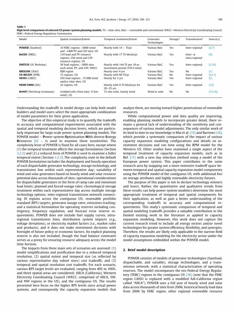
Table 1High level comparison of selected US power system planningmodels. TS¼ time-slice. R&C¼ renewable and conventional. WECC¼Western Electricity Coordinating Council.FERC¼Federal Energy Regulatory Commission.
Model Spatial resolution/Extent Temporal resolution/Extent GeneratorTechnologies
Storage? Transmission? Source(s)
POWER (Stanford) 10 FERC regions; ~6000 windand ~1400 PV and CSP sites; US
Hourly with 14 þ TS/yr Various R&C Yes Inter-regional [6,7]
ReEDS (NREL) 134 load and PV resourceregions; 356 wind and CSPresource regions; US
Hourly with 17 TS blocks/yr Various R&C Yes Inter- &intra-regional
Hourly with 144 TS per 10-yrinvestment period (576 h total)
Various R&C Yes Inter-regional [2,10]
RREEOM (UDel) PJM region Hourly over 4 yrs Various R&C Yes No [1]US-REGEN (EPRI) 15 regions; US Hourly with 86 TS/yr Various R&C No Inter-regional [4,11]NEWS (CIRES) 256 load regions; ~37,000 wind
and/or solar sites; USHourly for 3 yrs Various R&C Yes Inter-regional [5]
NEMS EMM (EIA) 22 regions, US Hourly with 9 TS blocks/yr for20e25 yrs
Various R&C Yes Inter-regional [12]
ReNOT (Northrop Grumman) Gridded cells (4 km solar, 12 kmwind), US
15 min solar, hourly wind Wind & solar No No [13,14]
B.A. Frew, M.Z. Jacobson / Energy 117 (2016) 198e213 199
Understanding the tradeoffs in model design can help both modelbuilders and model users select the most appropriate combinationof model parameters for their given application.
The objective of this empirical study is to quantify the tradeoffsin accuracy and computational requirements associated with thespatial and temporal modeling decision levers, which are particu-larly important for large-scale power system planning models. ThePOWER model e Power system Optimization With diverse EnergyResources [6] e is used to examine these sensitivities. Thecomplexity lever of POWER is fixed for all cases here, except where(1) the temporal treatment affects the storage formulation (Section3.2.2) and (2) a reduced form of POWER is used to examine a fullertemporal extent (Section 3.2.3). The complexity state in the defaultPOWER formulation includes the deployment and hourly operationof each dispatchable generator technology, storage technology, andtransmission line within each representative day; variability ofwind and solar generators based on hourly wind and solar resourcepotential data across thousands of sites; operational considerationsfor dispatchable generators in the form of ramp rate and minimumload limits; planned and forced outage rates; chronological storagetreatment within each representative day across multiple storagetechnology options; inter-regional transmission network connect-ing 10 regions across the contiguous US; renewable portfoliostandard (RPS) targets; generator outage rates; emissions tracking;and a statistical formulation for operating reserves including con-tingency, frequency regulation, and forecast error reserve re-quirements. POWER does not include fuel supply curves, intra-regional transmission lines, distribution system impacts (e.g.,voltage deviations), or electricity market factors (i.e., market rulesand products), and it does not make investment decisions withforesight of future policy or economic factors. An explicit planningreserve is also not included, though the load balance constraintserves as a proxy for ensuring resource adequacy across the modeltime horizon.
The impacts from three main sets of scenarios are assessed: (1)model simplifications and justification due to a reduced temporalresolution, (2) spatial extent and temporal size (as reflected byvarious representative day subset sizes) cost tradeoffs, and (3)temporal and spatial resolution cost tradeoffs. For each scenario,various RPS target levels are evaluated, ranging from 40% to 100%,and three spatial areas are considered: AllCA (California), WesternElectricity Coordinating Council (WECC, comprised of AllCA, SW,and NW regions in the US), and the contiguous US. The resultspresented here focus on the higher RPS levels since actual powersystems, and consequently the capacity expansion models that
analyze them, are moving toward higher penetrations of renewableresources.
While computational power and data quality are improving,enabling planning models to incorporate greater detail, there re-mains a general lack of understanding of the sensitivity and con-sequences of various model adjustments. The only similar work ofits kind to date to our knowledge is Mai et al. [15] and Barrows [16],which provide a systematic comparison of the impact of variouscapacity expansion modeling configurations and details on in-vestment decisions and run time using the RPM model for theWestern US. Other studies have examined a single aspect of thetemporal treatment of capacity expansion models, such as inRef. [17] with a new day selection method using a model of theEuropean power system. This paper contributes to the sameresearch area by mapping out a more extensive tradeoff space be-tween temporal and spatial capacity expansion model componentsusing the POWER model of the contiguous US, with additional focion storage attributes and highly renewable electricity futures.
The purpose of this paper is not to declare technology winnersand losers. Rather, the quantitative and qualitative trends fromthese results can help power system modelers determine the mostappropriate treatment of temporal and spatial components fortheir application, as well as gain a better understanding of thecorresponding tradeoffs in accuracy and computational re-quirements. This study's systematic comparison of temporal andspatial modeling tradeoffs provides a valuable contribution to thelimited existing work in the literature as applied to capacityexpansion modeling. However, this work does not capture thecurrent research trend to include all energy sectors and/or noveltechnologies for greater system efficiency, flexibility, and synergies.Therefore, the results are likely only applicable to the narrow fieldof capacity expansion modeling for the electricity sector under themodel assumptions embedded within the POWER model.
2. Brief model description
POWER consists of models of generator technologies (baseload,dispatchable, and variable), storage technologies, and a trans-mission network, with a statistical characterization of operatingreserves. The model encompasses the ten Federal Energy Regula-tory (FERC) regions in the contiguous US [18] (note that the FERCregion CAISO is replaced with a modified full-California regioncalled “AllCA”). POWER uses a full year of hourly wind and solardata across thousands of sites from 2006, historical hourly load datafrom 2006 by FERC region, other regional renewable resource
B.A. Frew, M.Z. Jacobson / Energy 117 (2016) 198e213200
availability data, regional cost parameters and various systemparameter inputs to solve deterministically for the least-costportfolio of generators, storage, and transmission that meet theelectric load in each hour of the year while attaining a given RPStarget. POWER uses these single year data inputs to construct afuture electricity system with no definite time stamp and with noconstraints imposed by the existing infrastructure (i.e., “greenfield”approach) except for the inclusion of existing transmissioncorridors.
Each system component has an annual cost that is a function ofthe amortized capital costs that depend on the installed capacitydecision variables, and the annual variable costs that depend on thetotal annual generation or storage throughput. A key model outputis the total annual system cost, which is the total amortized costs ofall generators, storage technologies, and transmission capacity andaccounts for both fixed and variable costs, aggregated across therespective spatial extent. Total annual cost is the metric of choicefor this study since it combines both the capacity and energy as-pects of the system.
POWER decides how much capacity to build of each systemcomponent and how those components should be dispatched eachhour. Wind and solar sites are evaluated individually, but all othercomponents are aggregated by FERC region. POWER includes asimplified representation of three storage technologies: pumpedhydroelectric storage, concentrating solar power with thermalenergy storage (CSP TES), and a generic battery storage option thatis indicative of the current and future range of stationary batterystorage technologies. However, as noted in Ref. [6], CSP is notdeployed in most scenarios evaluated with POWER due to its lessfavorable economics. Each storage technology is characterized byenergy conversion efficiencies into and out of storage and the lossesduring storage. Unless otherwise noted, the results in this study arebased on 8 h of storage duration. The relevant storage costs in thetotal annual system costs include the power and/or energy capacitycosts, which are applied to the size of the storage system built, andthe variable operations and maintenance cost (VO&M), which isapplied to the energy throughput.
Additionally, there are optional submodels to include existinggenerators, generator retirements based on age and environmentalregulations, and additional firm and flexible load from plug-inelectric vehicle (PEV) charging. However, expect for a set of sensi-tivity runs in Appendix A, the results presented in this study do notconsider the impact of PEV charging; see Ref. [6] for an investiga-tion of the flexibility impacts of this feature. Responsive demand,new load from additional electrified sources (e.g., industrial pro-cesses and all other energy sectors), and applications for utilizingotherwise curtailable energy (e.g., district heating, irrigationpumps, water desalination/purification, and other forms of storage,such as hot and chilled water, ice, rocks, phase-change materials,and chemicals, including hydrogen) are not modeled. Emissionsfrom fossil fuel generators are also quantified. See Chapter 4 inRef. [7] for the full model formulation and input data details. Theresults presented in this study were run on a shared server with 19nodes, 24 cores per node and 96 GB RAM per node.
A growing body of research is incorporating the above all-sectorenergy impacts and curtailment-reducing options into highlyrenewable energy system modeling analyses. For example, Jacob-son et al. [19] used the LOADMATCH grid integration model to solvefor a 100% wind, water, and solar resource-powered contiguous USgrid to supply energy to all end-use sectors, including electricity,transportation, heating/cooling, and industry. LOADMATCH is atrial-and-error model that marches forward in time, which differsfrom the optimization-based POWER model that considers manytime steps simultaneously. The study also considered flexibilityoptions from various storage options that utilize a variety of
thermal, materials, and mechanical processes, as well as flexibleelectrified loads from transportation, industrial and chemical pro-cesses. Connolly et al. [20] implemented a similar full-systemapproach, but using a step-wise process to convert to a fullyrenewable European system by 2050. Each step involves a fuelswitch, load electrification, or other energy-saving transition. Theholistic approach of connecting the electricity, heating, cooling, andtransport sectors together enables greater system flexibility andefficiency. Future work should incorporate these aspects into thePOWER model and tradeoff analyses of modeling methods.
3. Tradeoffs and sensitivities of temporal modelingsimplifications
Ideally, large-scale capacity expansion models would be runserially for all hours in a year to capture the time-linked behavior ofstorage and to avoid omission of any solution-constraining hour(s).However, such temporal treatment is often computationallyintractable. Three types of methods were explored to reduce thetemporal size and/or resolution of POWER: (1) warmstarting withindependent time periods and model predictive control, (2)implementing an alternating direction method of multipliers(ADMM) algorithm, and (3) running the full model with a reducednumber of hours. Each of these options resulted in a loss of accu-racy, in some cases at unacceptable levels. The first two methodswere ruled out due to computational intractability (warmstarting)or accuracy losses (ADMM). Details on these methods and resultsare provided in Section 4.10 of [7].
In the third method e running the model for a reduced numberof hours e two cases were evaluated: (1) using a coarser temporalresolution of all days within a year, and (2) using a representativesubset of days from a full year. Similar, but varying, methods havebeen used in most other large-scale capacity expansion models toselect a representative subset of hours or “time-slices.” Theseinclude peak and median load-based days fromwithin each month(SWITCH), aggregate time-slices across each season plus a summer-peak time-slice (ReEDS), and extreme events within “bubbles” ateach of the eight Euclidean corners of the joint load-wind-solardistributions with additional hours to represent base and shoul-der events (US-REGEN).
3.1. Coarser temporal resolution
The first set of reduced-hours model modifications included alldays of the year with reduced temporal resolutions in POWER. Theresolutions considered were every 2 h, 4 h, and 8 h across the fullyear. The time series data for these runs were created by averagingall hourly values within each time step block. POWER maintainedfull chronological treatment in these runs, with uniform time stepweights equal to the time step size (e.g., weight of 2 for 2 hourlyresolution). Results from these model instances are presented inthe temporal resolution results in Section 4.2.
3.2. Representative subset of days
The second reduced-hours modification used a representativesubset of days within a full-year temporal extent. This modificationresults in the loss of chronology across all resulting hours. Instead,chronology is maintained only among the hours within eachrepresentative day. POWER still looks across the full temporalextent of one year for capacity decisions, however.
The sensitivity of the model to the day selection method andassociated storage model modifications are investigated in Sections3.2.1 and 3.2.2, respectively. The impacts of these modeling modi-fications are then quantified and justified with a reduced form
B.A. Frew, M.Z. Jacobson / Energy 117 (2016) 198e213 201
model of POWER in Section 3.2.3. The full version of POWER with arepresentative subset of days was used for all results in Section 4,except the temporal resolution results in Section 4.2.2.
3.2.1. Day selection methodThe representative subset of days for POWER include “extreme”
event days (high and low), and if desired, additional days selectedrandomly to represent “typical” system behavior. Extreme dayscontain themaximumhour along each of the eight vectors from theorigin to the vertices of a unit cube, based on normalized hourlywind and solar (averaged across all potential developable sites) andload data for a full year for each region and interconnected aggre-gate area. Extreme days are first selected, and then random“typical” days are added until the desired number of total days isreached. In this way, the most constraining instances are firstincluded so that a more (or equally) optimal solution is obtained asrandom days are added. In order to calculate annual total values,weights were then assigned to each selected day using least-squares to best match the full-year wind, solar, and load distribu-tions. One important caveat is that these weights are based on themaximum hourly production across all wind and solar sites andonly the historic hourly load; they are not updated based on anynew wind or solar builds or modified load shapes. Additional stepswere implemented for scenarios with interconnected regions tofurther reduce the representative subset of days into amore concisesubset; various methods were tested to determine the best optionfor different spatial extents. More details on this methodology andcorresponding sensitivity results are provided in Sections S1.1 andS1.2 of Appendix A.
The main finding from the comparison of different day selectionmethods for interconnected regions is that the model outputs aresensitivee for some spatial extents and casesmore than otherse tothe subset of days included in the temporal extent. For example,results from the interconnected WECC region yielded <15% differ-ence in total cost, but up to double the renewable overgenerationvalues, between different day selection methods and subset sizes(see Section S1.2). The key is to capture the extreme events dayswithout over-representing their impact on the system performance(e.g., renewable overgeneration and energy production). Similarobservations of this sensitivity to the day selection methodologywere noted by the US-REGEN model [21] and in a paper presentinga methodology for selecting representative days based on a modi-fied hierarchical clustering technique [17]. Possible methods ofaddressing this issue include clustering algorithms such as k-meansor hierarchical clustering, which have shown success in findingrepresentative subsets of electric load data (e.g. [22], using load andwind data with validation against full-year data, and [23] using anorder-specific clustering algorithm to accommodate sequentialload data, while preserving its daily fluctuations) and jointly forelectricity prices and solar irradiation data [24]. A thorough dis-cussion of temporal sampling methods, including a robust appli-cation of the “Ward’s” clustering algorithm, as well as moregeneralized approaches such as those using netload durationcurves, is provided in [25].
3.2.2. Sensitivity to storage model modificationsThe baseline version of POWER uses a representative subset of
days that are distributed throughout a full year. Because of thistemporal disjointedness, the chronological tracking of storage islimited to the 24 h within each representative day. To deal with theseams between the days, a periodic boundary constraint is appliedto each representative day so that POWER chronologically tracksthe amount of storage going into, out of, and held in storage foreach time step within each day. Each storage technology is trackedseparately and represents the aggregate capacity of that technology
within each spatial region (i.e., individual battery sites are notmodeled). The model results are sensitive to the way in which thisperiodic boundary constraint is applied. Existing methods tohandle this discontinuity focus on balancing the storage energyover each day, either by requiring that (1) the sum of the net storagevalues equal zero each day (e.g., [2]), or (2) the amount of energyheld within storage is the same at the start and end of the day (e.g.,[26]). These methods are described more fully in Section S1.3 inAppendix A.
A comparison of the performance of these two methods underdifferent storage balancing conditionswasmade using the subset ofdays from Section 3.2.1 for highly renewable AllCA and WECCsystems. These storage balancing conditions included summing thenet storage values to zero each day (method 1), as well as differentcapacity levels to start/end each day (method 2). The results be-tween all of these conditions generally yielded <3% difference intotal annual system cost. A comparison of these conditions forAllCAwith PEV load and 56 representative days at an 80% RPS levelis shown in Fig. S5 in Appendix A; the storage component of thissystem consists of about 12 GW power capacity and 93 GW-hrenergy capacity of pumped hydro storage, corresponding to about8% of the total system installed capacity. However, the best optionon the combined bases of cost, renewable overgeneration, run time,and daily storage profile is to require that the system holds thesame amount of energy within storage at the end of each day(method 2) at a level chosen endogenously by the model. SeeSection S1.3 in Appendix A for more details on these results. Thisstorage model modification was implemented in all final modelruns that used a representative subset of days in Section 4.
To assess the sensitivity of POWER to the daily storage balanceconstraint, the chosen daily storage balance constraint was thencompared with the original full chronological treatment for aspringtime period of 77 days. As shown in Figs. S6eS7 in AppendixA, constraining storage to balance each day yielded very similarsystem portfolio and total system costs (<2% difference) as the fullchronological version. However, the daily storage balanceconstraint case yielded noticeably more renewable overgeneration,more ramping of generators, and greater throughput in storagethan allowing inter-daily storage flows (chronological version),especially in a fully renewable AllCA system. See Section S1.4 inAppendix A for more details on these results.
The sensitivity of themodel to the presence and/or choice of thisdaily balance constraint further highlights the significance ofproper temporal handling in power system planning and gridintegration models, especially at high RPS targets when storagetends to play a greater role. Awareness and proper treatment ofthese modeling features will therefore become more important ascapacity expansion models investigate higher penetrations ofrenewable resources. Ideally, a full-year serial model would be usedto capture a more accurate performance, and likely a greaterbenefit, from the seasonal and/or weekly flexibility that storage canprovide (e.g., a weekly storage cycle is observed in many pumpedhydro storage facilities). However, based on the results here, thesmall difference in system buildout and costs justifies the use of adaily storage balance constraint when the daily seams are properlyhandled and when computational limitations prevent the imple-mentation of a full-year serial treatment.
These storage sensitivity results reflect outputs with a simplestorage model for a limited suite of storage technologies. WhilePOWER does account for the diurnal and seasonal variations insolar resource supply for CSP TES, the results here do not reflectadditional sensitivities to the storage duration (assumed to be 8 h),diversity of battery storage options, or the impact that additionalstorage technologies, new load, or responsive demand might have.The results here are intended to highlight the importance of the
B.A. Frew, M.Z. Jacobson / Energy 117 (2016) 198e213202
way in which a storage balance constraint is applied with a simplestorage model in a highly renewable system when full chronolog-ical treatment is computational intractable.
3.2.3. Sensitivity to the number of representative daysTo examine the sensitivity of model accuracy and computational
requirements to the number of representative days implemented, areduced form model was created for the AllCA region. Thissimplified version of POWER contained only natural gas, wind(onshore and offshore with a uniform buildout across all sites),solar PV (large-scale and residential with a uniform buildout acrossall sites), battery storage, reserve requirements, and emissioncomponents from the original full model formulation. These sim-plifications enabled an ideal full-year serial run as a benchmark forcomparing the same full-year temporal extent with variousrepresentative day subset sizes (8e168 days) with the daily storagebalance constraint that was introduced in Section 3.2.2.
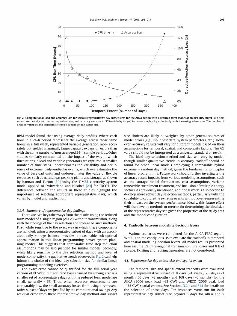
For each representative day subset size that included bothextreme and random days, ten instances were run and the resultsthen averaged. The extreme-only 8-day scenario and full-year serial365-day scenario each had only a single set of results. Fig. 1 displaysthe resulting total annual system cost, standard deviation of costacross the 10 instances, and renewable overgeneration for variousrepresentative day subset sizes for AllCA with an 80% RSP target.Fig. 2 plots the percent loss in objective function accuracy (totalsystem cost) relative to the 365-serial-day target, as well as thecomputational load measured as CPU run time, for these samerepresentative day subset sizes. For comparison, the maximummemory usage (not shown) also scales roughly quadratically withthe number of days, requiring about 55 GB of RAM in the 365-serial-day instance.
The total cost, standard deviation of cost, accuracy loss, andrenewable overgeneration all decrease with increasing represen-tative day subset size, each approaching the target 365-serial-dayresult. This trend is only approximate, due to the variation inrandomly selected days, especially at lower subset sizes where thestandard deviation is higher. Nevertheless, these results reveal thediminishing returns in accuracy (roughly logarithmic) andincreasing computational run time (quadratic) with increasing
Fig. 1. Total annual system cost and renewable overgeneration for various representatitarget. Values for 8 days are based only on the most extreme wind, solar, and load events. Vawhich include the same 8 extreme days plus additional random days. Total costs (2006USD
subset size. For comparison, the maximum memory usage alsoscales roughly quadratically. The loss in objective function accuracywas generally�6% for the representative day subsets of all extremeplus some random days (i.e., 14 þ days).
The quadratic run time observations from this reduced formversion of POWER is supported by well-documented findings fromearly work with the simplex method, which show that linear pro-grams can generally be solved in “polynomial-time” [27] or in somecases “exponential-time” [28]. See Section S15 in Appendix A for asimple qualitative example that helps to describe these computa-tional run time trends.
Few papers have evaluated the tradeoffs in accuracy and/or runtime with various modeling structures as applied to power systemplanning. Among them, Nahmmacher et al. in Ref. [17] similarlycompared cost versus the number of representative days using theLIMES-EUmodel of the European power system. Their total systemcost results, however, increased with increasing subset size,whereas those with POWER decreased. The reason is discussedshortly. Similarly, Nicolosi [29] compared overgeneration by thenumber of time slices using an investment and dispatch model ofERCOT and found that overgeneration increased with a largernumber of time slices; the opposite trend was observed with PO-WER in Fig. 1. The difference between the results from Nahm-macher et al. and Nicolosi and those here in Fig. 1 can be attributedto the absence or limited inclusion of extreme days in their dayselection methodology. Conversely, the day selection method inPOWER begins with extreme days and incorporates more random“typical” days with increasing subset size, consequently yieldingmore cost-effective systems and lower overgeneration. Thisobservation follows linear programming theory, by which a subsetof the full problem (solution space) will yield a suboptimal (or equalto the optimal) solution.
Similar accuracy and run time results as those in Fig. 2 wereshown in Mai et al. [15], who found that increasing the number ofhours included in the dispatch period from 24 h to 96 h increasedcomputational run time by nearly 2 orders of magnitude (fromabout 1.5 h to 7 days, respectively), with little impact on the in-vestment decisions using the RPM model of the US WesternInterconnection. Follow-on work by Barrows et al. [16] with the
ve day subset sizes for the AllCA region with a reduced form model at an 80% RPSlues for all other days (except 365-serial-days) are based on the average of 10 runs each,) are shown above bars, and error bars correspond to standard deviation of total costs.
Fig. 2. Computational load and accuracy loss for various representative day subset sizes for the AllCA region with a reduced form model at an 80% RPS target. Run timescales quadratically with increasing subset size, and accuracy (relative to 365-serial-day target) increases roughly logarithmically with increasing subset size. The number ofdecision variables and constraints strongly depend on the subset size.
B.A. Frew, M.Z. Jacobson / Energy 117 (2016) 198e213 203
RPM model found that using average daily profiles, where eachhour in a 24-h period represents the average across those samehours in a full week, represented variable generation more accu-rately but yielded marginally larger capacity expansion errors thanwith the same number of non-averaged 24-h sample periods. Otherstudies similarly commented on the impact of the way in whichfluctuations in load and variable generators are captured. A smallernumber of time steps underestimates the variability and occur-rence of extreme load/wind/solar events, which overestimates thevalue of baseload units and underestimates the value of flexibleresources such as natural gas peaking plants and storage, as shownby Kannan and Turton [30] using the TIMES electricity systemmodel applied to Switzerland and Nicolosi [29] for ERCOT. Thedifferences between the results in these studies highlight theimportance of selecting appropriate representative days, whichvaries by model and application.
3.2.4. Summary of representative day findingsThere are two key takeaways from the results using the reduced
form model of a single region (AllCA) without transmission, alongwith the findings of the day selection and storage balance methods.First, while sensitive to the exact way in which these componentsare handled, using a representative subset of days with an associ-ated daily storage balance provides a reasonable sub-optimalapproximation in this linear programming power system plan-ning model. This suggests that comparable time step reductionassumptions may be also justified for similar models. Secondly,while likely sensitive to the day selection method and level ofmodel complexity, the qualitative trends observed in Fig. 2 can helpinform the choice of the ideal day selection size for similar linearprogramming modeling exercises.
The exact error cannot be quantified for the full serial yearversion of POWER, but accuracy losses caused by solving across asmaller set of representative days with the reduced formmodel aresmall, generally �6%. Thus, when accuracy requirements arecomparably low, the small accuracy losses from using a represen-tative subset of days are justified by the computational savings. Anyresidual error from these representative day method and subset
size choices are likely outweighed by other general sources ofmodel errors (e.g., input cost data, system parameters, etc.). How-ever, accuracy results will vary for different models based on theirassumptions for temporal, spatial, and complexity factors. This 6%value should not be interpreted as a universal standard or result.
The ideal day selection method and size will vary by model,though similar qualitative trends in accuracy tradeoff should befound for other linear models employing a comparable hybridextreme þ random day method, given the fundamental principlesof linear programming. Future work should further investigate theaccuracy result impacts from various modeling assumptions, suchas the storage model formulation, cost assumptions, variablerenewable curtailment treatment, and inclusion of multiple energysectors. As previously mentioned, additional work is also needed todevelop more robust day selection methods, particularly with thecapability to capture the extreme events without over-representingtheir impact on the system performance. Ideally, this future effortwill also develop methods or metrics for determining the ideal sizeof the representative day set, given the properties of the study areaand the model configuration.
4. Tradeoffs between modeling decision levers
Various scenarios were completed for the AllCA FERC region,WECC, and the contiguous US to evaluate the tradeoffs in temporaland spatial modeling decision levers. All model results presentedhere assume 5% intra-regional transmission line losses and 8 h ofstorage. Existing and retiring generators are not considered.
4.1. Representative day subset size and spatial extent
The temporal size and spatial extent tradeoffs were evaluatedusing a representative subset of 8 days (~1 week), 28 days (~1month), 56 days (~2 months), and 168 days (~6 months) for theAllCA (2006 peak load ~62 GW) and WECC (2006 peak load~133 GW) spatial extents. See Sections 3.2.1 and S1.1 for details onthe selection of these days. Ten instances were run for eachrepresentative day subset size beyond 8 days for AllCA and 5
B.A. Frew, M.Z. Jacobson / Energy 117 (2016) 198e213204
instances for each extent beyond 22 days for WECC. All resultspresented here are the averages of those instances. Additionalspatial extent results are presented for the full contiguous US (2006peak load ~729 GW). All runs in this section include the dailystorage balance constraint (Section 3.2).
Fig. 3 summarizes the total annual system cost for each tem-poral and spatial extent combination for AllCA and WECC. Alsoshown are the percent increases in cost relative to the most “ideal”computationally tractable combination in each spatial extent col-umn (open star). The most ideal representative day subset size foreach column is a full year (filled star), but this was computationallyintractable. The spatial extent columns (from left to right) representthe AllCA region individually, the sum of independent WECC con-stituent regions (AllCA, NW, and SW), and the interconnectedWECC region. Each increasing spatial extent required greatercomputational resources, which reduced the maximum achievablerepresentative day subset size.
On the spatial extent axis, the total cost was sensitive to theimpact of geographic aggregation. This is reflected by the differencebetween the sum of WECC regions and the interconnected WECC,with roughly a 14% reduction in total cost due to interconnection
Fig. 3. Temporal and spatial extent cost tradeoffs for AllCA and WECC regions at an 80%in cost in italics relative to the most “ideal” computationally tractable case within each spatifor a full year of days (filled star), but this was computationally intractable.
for the 56 representative day subset size. Additional runs for thecontiguous US (Section 4.1.2) reveal that the benefits of aggregationare increased for larger spatial extents and RSP targets, achievingtotal cost reductions of about 42%. The reliability and cost benefitsof aggregation are well-documented for cases where geographicareas are interconnected, allowing for access to a greater diversityof resources and reserves (e.g. [31], with an extension of theWestern US Energy Imbalance Market and [32] with a US-basedwind study). This study reveals that the cost trends withincreasing spatial extent are driven by these aggregation benefitsrather than by an underlying computational tradeoff.
4.1.1. Representative day subset sizeAs shown in Fig. 3, the total cost decreased as the representative
day subset size increased, since the smaller subset sizes containdisproportionally more high-load hours (see Sections 3.2.1 andS1.1). Increasing the size of the subset by adding more random“typical” days resulted in an increasingly more accurate represen-tation of the full year.
The representative day subset sizes in Fig. 3 followed the samehigh-level trends as the reduced form model in Section 3.2.3 for
RPS target. Total annual system cost (Billions of 2006USD/year), with percent increaseal extent column (open star). The ultimate goal is to model each spatial extent category
B.A. Frew, M.Z. Jacobson / Energy 117 (2016) 198e213 205
total cost, standard deviation of total cost, renewable over-generation, and tradeoffs in computational requirements and ac-curacy (see Figs. S9eS13 in Appendix A). In the AllCA system, 56days provided the best combination of accuracy, computationalrequirements, and system configuration and operation. Because thestandard deviation of total cost was very small, any single instancefrom among the ten 56-day runs would suffice, but the mostrepresentative instance was used for all subsequent AllCAscenarios.
A similar representative day subset size threshold was deter-mined to be suitable for a large-scale linear optimization model ofthe European electricity system [33]. They found that computationslimited to 6 typical weeks (42 days) were sufficient; a sensitivityanalysis with larger subset sizes did not significantly changeresults.
For the larger spatial extent ofWECC, 28 dayswas determined tobe the ideal representative day subset size. Similar observationswere made for these WECC cases as with the single AllCA region.See Section S2.2 in Appendix A for details on these AllCA andWECCresults.
4.1.2. Spatial extentThe sensitivity to spatial extent was examined by comparing the
total system cost breakdown and renewable overgeneration of theindependent constituent WECC regions against the interconnectedWECC case at 50% and 80% RPS targets (Fig. 4). Region-specificdetails of these results are shown in Figs. 5 and 6 for the inde-pendent regions and Figs. 7 and 8 for the interconnected scenario.
The cost breakdown in Fig. 4 reveals that the interconnectedcase deployed less solar, wind, and storage than the independentregion case for both RPS targets. At a higher RPS target, there wassignificantly more renewable overgeneration in both the inter-connected and independent cases, as compared to the lower RPStarget. However, the interconnected case saw greater relative costand overgeneration savings in the higher RPS target case. Addi-tionally, as RPS requirements increased, wind was built out beforesolar, especially in the interconnected system. These findings agreewith the base case results of a WECC study using the SWITCHmodel [2], although the SWITCH model installed small amounts ofcoal and nuclear, while the results here had none of either.
New transmission capacity occupied a small fraction of theinterconnected system total cost. Both the 50% and 80% RPS inter-connected WECC scenarios utilized transmission, but only the 80%
Fig. 4. Total annual system cost and renewable overgeneration for independent WECCvalues are for cases with a representative subset of 56 days. Costs are in 2006USD.
case required new additional capacity, representing about 1% of thetotal cost. This finding roughly agrees with other grid integrationstudies of the western US, such as that using the SWITCH model[34] and that using the WREZ model [35], which found that newand existing transmission costs represent less than 10e19% of thetotal cost for a highly renewable system. Transmission costs pre-sented herewere reasonably smaller since they were based only onnew (and not total) capacity. To calculate the regional transmissioncosts in POWER, the cost for each transmission segment wasassumed to be split evenly between the two end node regions.
The wind and solar site buildouts, transmission flows, relativecost contributions (Figs. 5 and 7), and system performance (Figs. 6and 8) between the independent regions and interconnected sce-narios reveal several important differences in the effect of aggre-gation as part of the spatial extent spectrum. The first differencewas the disproportionate contribution of the constituent regions tothe aggregate RPS, suggesting the need for region-and-resource-specific RPS targets. An 80% aggregate RPS does not necessarilymean that each regionwill achieve an 80% RPS. In fact, in the resultsof this WECC system, both AllCA and SW built and used morenatural gas generators in the aggregated case, resulting in lowerregional achieved RPS targets (67% and 75%, respectively) ascompared to the independent region case (each at 80%). The NWregion compensated for this in the aggregated case by becomingfully renewable and transmitting excess generation (Fig. 8). Thedominate presence of hydro in the NW region poses a potentialreliability risk in the event of reduced hydro flows due to drought orother causes.
Secondly, there was less solar deployment in the aggregatedcase. This was especially apparent in the performance time seriesplots (Figs. 6 and 8). All developed solar capacity was large-scalePV; no residential PV was built in any cases, including othermodel scenarios of the contiguous US, which are discussed shortly.Large-scale PV is an abundant, comparatively lower-cost resource,precluding the need for any residential PV with this modelformulation. However, this does not suggest that residential PVshould be disregarded for highly renewable systems. For example, ifthe intra-regional transmission and distribution line losses andcapacity savings are considered, then residential PV may become amore cost-effective option. These benefits are outside of the spatialresolution captured by POWER, but separate sensitivity analyses ofthe US and AllCA systems with POWER revealed that a 40e45%reduction in residential PV costs resulted in the displacement of
regions vs. interconnected WECC (AllCA, SW, NW) for 50% and 80% RPS targets. All
Fig. 5. Breakdown of total annual system cost and wind and solar site buildouts for independent WECC regions (AllCA, SW, NW) at an 80% regional RPS target. Pie chartsshow relative contribution of each built generator and storage technology to the total annual cost in each region. Actual achieved RPS in each region is shown in pie charts; averageof all regions is shown at bottom. Results are based on a representative subset of 56 days.
Fig. 6. Zoom-in to 8 days of system performance for independent WECC regions at an 80% RPS target. Days shown are from the months of June and July (from a representativesubset of 56 days) and correspond to results shown in Fig. 5.
B.A. Frew, M.Z. Jacobson / Energy 117 (2016) 198e213206
roughly 10e18% of large-scale PV capacity and about 2e7% of windcapacity by residential PV, relative to an 80% RPS target base casewithout PEV load. In these sensitivity cases, the extreme short-duration events caused by the overall larger share of coincidentsolar production resulted in a greater need for system flexibility,fulfilled by storage and curtailment (see Ref. [6] and Section 5.4 inRef. [7]).
Third, based on these results from the western US with POWER,aggregating regions through an enhanced transmission system iseconomically more favorable than only harnessing local resources
coupled with storage. Storage was still used, but to a significantlylesser degree, especially at higher RPS targets. For instance, in theWECC scenarios with an 80% RPS target, energy from pumpedhydro storage met about 3% of the total load in the independentregions case, but only 0.2% in the aggregated case, with trans-mission instead providing 6% of the total load in the latter case.Transmission occupied <1% of the total cost in this WECC scenario.The dominant transmission flows agreed relatively well with thefindings from the SWITCH model [2], where a net flow from windgeneration in the SW was transmitted to the NW, net flow from
Fig. 7. Breakdown of total annual system cost, wind and solar site buildouts, and net transmission flows for interconnected WECC with an 80% aggregate RPS target. Piecharts show relative contribution of each built generator and storage technology to the total annual cost in each region. Arrow show dominant direction of transmission flow, andweight of line shows relative magnitude of net flow. Actual achieved RPS in each region is shown in pie charts; actual aggregate RPS is shown at bottom. Results are based on arepresentative subset of 56 days.
Fig. 8. Zoom-in to 8 days of system performance for interconnected WECC regions at an 80% RPS target. Days shown are from the months of June and July (from a repre-sentative subset of 56 days) and correspond to results shown in Fig. 7. Note the difference in color bars between Fig. 6 and this figure.
B.A. Frew, M.Z. Jacobson / Energy 117 (2016) 198e213 207
hydro in the NWwas transmitted to AllCA, and net generation fromsolar and wind in the SW was transmitted to AllCA. However,noticeably less solar was installed in the SW region with POWER.
To determine if these same aggregation effects transfer to therest of the US, POWER was then run with a subset of 14 days for allten FERC regions, both independently and as an interconnected
entity comprising the full contiguous US, at 80% and 100% RPStargets. This reduced representative day subset size was necessarydue to the significant increase in computational memory re-quirements with the larger US system. The resulting total costbreakdown by system component is shown in Fig. 9 for indepen-dent FERC regions and in Fig. 10 for the interconnected scenario.
Fig. 9. Breakdown of total annual system cost and wind and solar site buildouts for All FERC regions at 1000% RPS target. Pie charts show relative contribution of each builtgenerator and storage technology to the total annual cost in each region. Actual achieved RPS in each region is 100%. Results are based on a representative subset of 14 days.
B.A. Frew, M.Z. Jacobson / Energy 117 (2016) 198e213208
Similar observations weremade for the contiguous US system asfor WECC. First, transmission occupied a small portion at roughly5% of the total cost for both RPS targets. This was more than theWECC case and was primarily due to the need for enhanced east-west and ERCOT connections. Secondly, as observed in the WECCcase, the interconnected system had less solar and storagedeployment. Instead, the interconnected US system utilized morewind, especially in the Great Plains, Rocky Mountains, and PacificNorthwest (Fig. 10). Third, based on these results for the US, whichagree with those for the WECC spatial extent, enhancing thetransmission system to access a greater diversity and quality ofresources from larger geographic areas was more economicallyfavorable than accessing only local resources with increased stor-age. In the independent regions case, storage coupled with large-scale PV was especially prevalent in the eastern half of the US.
Note that the large presence of storage, particularly batterystorage, is also complemented by large transmission interchanges.These results do not single out transmission or storage as beingsuperior to the other, but rather that both are needed in differentcombinations depending on the existing infrastructure, regionaldemand, and regional resource mix. The decision to build largequantities of storage in these cases reflects the need for greatersystem flexibility. In practice, this flexibility could come from otherstorage technologies, responsive demand, or new load sources. Theimpact of flexible load e in the form of flexible load from PEVcharging with comparable scenarios in POWERe has been found to
further shift the system's economic preference from a moreregional basis with greater shares of relative storage to a moreaggregated, interconnected system with more dispersed renew-ables and less relative local storage [6]. Futurework should evaluatethe impact of a larger suite of flexible resources.
In these contiguous US scenarios, renewable overgenerationbecame increasingly significant at higher RPS targets. About 6% ofthe total wind, solar, and hydroelectric generation was curtailed inthe 80% RPS case and about 30% in the 100% RPS case. The NationalRenewable Energy Laboratory (NREL) Renewable Electricity Futuresstudy, which solved for the cost-optimal portfolio of generators,storage, and transmission using the ReEDS model, reflected similarresults for an 80% renewable US system. This NREL study found that8e10% of total solar, wind and hydroelectric generation was cur-tailed, almost all of which occurred in the western and easterninterconnects and varied by season [3].
Regional disparity was again seen in the level of renewablepenetration for an 80% aggregate RPS target. For the interconnectedUS, the ISONE, PJM, and SE regions all achieved less than the 80%target (57%, 56%, and 70%, respectively), while most other regionsbecome fully renewable to compensate. As seen in the WECC 80%RPS case, this disparity resulted in more natural gas generation inthe sub-performing regions (ISONE, PJM, and SE) compared to theindividual regions scenario.
The site buildout results shown here for the contiguous US alsoagree reasonably well with those from NREL's Renewable
Fig. 10. Breakdown of total annual system cost, wind and solar site buildouts, and net transmission flows for interconnected US with 100% aggregate RPS target. Pie chartsshow relative contribution of each built generator and storage technology to the total annual cost in each region. Arrow show dominant direction of transmission, and weight of lineshows relative magnitude of total annual net flow, with the largest magnitude being 389TWh from SPP to SE. Actual achieved RPS in each region, as well as the aggregate RPS, is100%. Results are based on a representative subset of 14 days.
B.A. Frew, M.Z. Jacobson / Energy 117 (2016) 198e213 209
Electricity Futures Study [3]. In NREL's study, wind was heavilyinstalled in the Great Plains, Great Lakes, Central, Northwest, andMid-Atlantic areas (roughly corresponding to the MISO, SPP, NWand PJM regions here), and solar was heavily installed in California,the Southwest, Texas, and the South (roughly corresponding toAllCA, SW, ERCOT, and SE regions here). Transmission buildout inthis NREL study was mainly east-west oriented, with key additionsto/fromERCOT, SE, SW, SPP, andMISO regions. These results suggestan emphasis on transmitting wind energy from the Great Plains tolarge-load, adjacent regions. The US results from the POWERmodel(Fig.10) were similar for wind and transmission, but solar wasmoreuniformly developed with POWER.
4.2. Temporal and spatial resolution
The temporal and spatial resolution tradeoffs were evaluated inAllCA for 50% and 80% RPS targets. Four temporal resolutions wereconsidered: time steps of every 1, 2, 4, and 8 h, each for a full-yeartemporal extent. The 1-h (“hourly”) resolution is based on arepresentative subset of 56 days due to computational limitationsas previously discussed. See Section 3.1 for details on the modelmodifications for the coarser time resolutions of 2, 4, and 8 h. Twospatial resolutions were evaluated for the buildout of wind andsolar sites: uniform buildout (i.e., each site within the region has
the same fractional development of the available resource) andindividual site buildout (i.e., the development of each site is aseparate decision variable).
Fig. 11 summarizes the total annual system cost for each tem-poral and spatial resolution combination and the percent increasein cost relative to the most “ideal” achievable combination of in-dividual sites at an hourly temporal resolution (open star). A sub-hourly temporal resolution is the ultimate goal (filled star), butsub-hourly data was not available for the entire contiguous US atthe time of this analysis.
Fig. 11 shows that, at a high RPS target (80%, shown on right), acoarser temporal resolution yielded a lower total annual systemcost for both uniform and individual site buildouts; the coarser theresolution, the lower the cost. At a medium RPS (50%, shown onleft), however, a coarser temporal resolution had comparativelylittle effect on the total cost. These differences are driven by thereduction inwind and solar variability due to averaging datawithineach time block. A less variable system (i.e., coarser temporal res-olution) requires less flexibility and is therefore less expensive. Thistrend was more pronounced at a higher RPS target (80%) wheremore wind and solar were deployed. At both RPS targets, the choiceof spatial resolution had a more significant effect on total cost. Theuniform buildout generally yielded a larger (suboptimal) total cost,especially in the high (80%) RPS case with a 9% increase in cost
Fig. 11. Temporal and spatial resolution cost tradeoffs for AllCA with 50% and 80% RPS targets. Total annual system cost (Billions of 2006USD/year) values are shown for eachresolution combination, and the percent increases in cost are shown in italics relative to the most “ideal” achievable case of hourly individual sites (open star). The ultimate goal is tomodel individual wind and solar sites at a subhourly temporal resolution (filled star), but subhourly data was not available. Hourly values are based on a representative subset of 56days, while coarser temporal runs are based on a full year of data.
B.A. Frew, M.Z. Jacobson / Energy 117 (2016) 198e213210
relative to the individual site buildout with an hourly temporalresolution.
4.2.1. Spatial resolutionFig. 12 displays two different spatial resolutions for wind and
solar site buildout with an hourly temporal resolution for AllCA at
Fig. 12. Wind and solar installed capacity by site for uniform and site-by-site buildouinstalled capacity at each site (note that the circle sizes have inconsistent scale between thdays. No offshore wind was built in the uniform case (left). Results correspond to the “hou
an 80% RPS target. Thesemaps reveal significant differences inwindand solar development between (1) considering each site inde-pendently for optimal site diversity, and (2) assuming an aggre-gated buildout across all sites uniformly as is done in some gridintegration studies (e.g., [1]). The site-by-site buildout results (rightside of Fig. 12) found that optimal wind and solar development is
t for AllCA at an 80% RPS target. The size of the buildout circles corresponds to thee different generator types). All values are for cases with a representative subset of 56rly” 80% RPS values in Fig. 11.
B.A. Frew, M.Z. Jacobson / Energy 117 (2016) 198e213 211
clustered in southern California. However, since POWER assumes a“copper plate” within each region, the cost of transmitting theaggregated output from these sites to the coastal load centers is animportant additional consideration that could alter these results.For example, results in Shawhan [36] indicate that the spatial res-olution of transmission-system detail in production cost modelscan impact greenhouse has emission results by as much as 20%.
A comparison of the breakdown of total annual costs betweenthe two spatial resolution categories for AllCA at various RPS targetsis shown in Fig. 13. At high RPS targets, the difference in cost andrenewable overgeneration become more pronounced betweenuniform buildout and site-by-site (“Indiv. Sites”) buildout, withabout a 10% reduction in cost and 20% reduction in overgenerationwith site-by-site buildouts at a 100% RPS target. These findingshighlight the benefit of modeling individual wind and solar sites foroptimal system planning in highly renewable energy futures.
4.2.2. Temporal resolutionThe breakdown of total annual costs across the four temporal
resolution categories (1-, 2-, 4-, and 8-h blocks) is shown in Fig. 14for AllCA at an 80% RPS target. As observed in the resolutionsummary matrix for this RPS target (Fig. 11), the total system costdecreases as the temporal resolution becomes coarser, with a dif-ference in cost of about 10% between the hourly (least coarse) and8-h (most coarse) cases. Fig. 14 reveals that the main driver of thistrend is the contribution from wind and solar. Additionally, acoarser temporal resolution significantly underestimates theovergeneration of renewables, with about an 85% difference inovergeneration between the hourly and 8-h cases. These results aredue to the loss of intra-time block variability as previously dis-cussed. The relatively large differences in cost and overgenerationand loss of variability with these reduced temporal resolutionscenarios suggest that the alternative temporal reduction option e
using a representative subset of days e provides a more accurateoverall representation of the system components and should be thepreferred method when computational limitations require areduced temporal treatment.
5. Summary and conclusions
This empirical study presents a link between various power
Fig. 13. Total annual system cost and renewable overgeneration comparison for wind anare based on a representative subset of 56 days. Costs are in 2006USD.
system modeling choices and their computational and accuracytradeoffs using the POWER least-cost optimization planning modelfor scenarios of a highly renewable US system. The first half of thestudy analyzed common temporal modeling simplifications,particularly the use of a representative subset of days within a full-year temporal extent. These days were selected as a combination ofextreme event and typical days. Low accuracy losses of generally�6% across various representative day subset sizes with a reducedform model of POWER suggest that using a subset of days is justi-fied by the associated computational savings. However, this accu-racy result is likely dependent upon the model formulation andcorresponding input assumptions, particularly with respect to thestorage model formulation, cost assumptions, variable renewablecurtailment treatment, and inclusion of multiple energy sectors.Across multiple scenarios, computational run time was found toincrease quadratically with increasing subset size, while accuracyincreased roughly logarithmically.
Because of the temporal disjointedness of most days in therepresentative subsets, the chronological tracking of storage waslimited to the 24 h within each representative day. Model outputswere found to be sensitive to the presence and/or choice of thisdaily balance constraint. While total system costs varied by <2%,the storage performance noticeably differed between a full chro-nological tracking of storage and the daily storage balanceconstraint. This highlights the need for proper temporal treatmentand daily/weekly/seasonal storage balancing constraints in powersystem planning models, especially at high RPS targets whenstorage tends to play a greater role. Overall, these temporal modi-fication findings suggest that using a representative subset of dayswith an associated daily storage balance provides a reasonable sub-optimal approximation in POWER.
The second half of this study quantified cost tradeoffs of varioustemporal and spatial modeling adjustments. These adjustmentsresulted in small changes of generally <15% in cost for the AllCAregion, WECC, and contiguous US. Summary matrices of thesetradeoffs can help model builders and users determine the mostappropriate treatment of temporal and spatial components fortheir given application. The most significant difference in total costwas due to the effect of aggregation across increasing spatial ex-tents, with about a 14% reduction in total cost for the WECC area atan 80% RPS target, and a 42% reduction for the contiguous US at a
d solar uniform and site-by-site buildouts for AllCA at various RPS targets. All values
Fig. 14. Total annual system cost and renewable overgeneration for various time step sizes (hours) for AllCA at an 80% RPS target. Costs are in 2006USD.
B.A. Frew, M.Z. Jacobson / Energy 117 (2016) 198e213212
100% RPS target. The impact of the spatial resolution of wind andsolar site development (individual site buildout versus uniformdevelopment across all sites) also had large impacts on total systemcost in the test case of the AllCA region. Compared to the uniformbuildout case, the site-by-site buildout case had about a 10%reduction in cost and 20% reduction in overgeneration at a 100%RPS target. These findings highlight the benefit of interconnectinglarge geographic areas and modeling individual wind and solarsites for optimal system planning in highly renewable energy fu-tures. In addition, total cost and overgeneration values wheresignificantly lower with a coarser temporal resolution due to adiminished representation of intra-time block variability, indi-cating that the use of a representative subset of days is thepreferred method when computational limitations require areduced temporal treatment.
The findings here reflect technically feasible scenarios for asimplified contiguous US electricity system and ignore many social,environmental, and political barriers, which may slow or preventactual implementation. The modeling tradeoff results presentedhere focused on capacity expansion modeling of the power systemwithout consideration of new technologies, new loads from othersectors that are currently not electrified, other applications thatcould use otherwise curtailed energy, or responsive demand. Theflexibility capabilities of these sources may impact the modelingtradeoff results presented here by, for example, re-defining“extreme days.” Additionally, since POWER finds the least-costportfolio and does not evaluate revenue streams, it cannot cap-ture the full value for all of the system components. This includesarbitrage for storage and flexible demand, as well as revenue op-portunities for generators in adjacent markets. Future work shouldexamine the impacts of these additional factors in the tradeoffsbetween the various decision variables. Future work should alsofocus on establishing a more robust day-selection method oralternative model formulations for reducing model run time andmemory requirements without sacrificing model accuracy.
Acknowledgements
BAF gratefully acknowledges financial support from a NationalDefense Science and Engineering Graduate (NDSEG) fellowship, aNational Science Foundation (NSF) graduate research fellowship,
and a Stanford University Charles H. Leavell Graduate StudentFellowship. The authors also thank Mary Cameron for valuablefeedback on the draft of this paper.
Appendix A. Supplementary data
Supplementary data related to this article can be found at http://dx.doi.org/10.1016/j.energy.2016.10.074.
References
[1] Budischak C, Sewell D, Thomson H, Mach L, Veron DE, Kempton W. Cost-minimized combinations of wind power, solar power and electrochemicalstorage, powering the grid up to 99.9% of the time. J Power Sources 2013;225:60e74. http://dx.doi.org/10.1016/j.jpowsour.2012.09.054.
[2] Nelson J, Johnston J, Mileva A, Fripp M, Hoffman I, Petros-Good A, et al. High-resolution modeling of the western North American power system demon-strates low-cost and low-carbon futures. Energy Policy 2012;43:436e47.http://dx.doi.org/10.1016/j.enpol.2012.01.031.
[3] National Renewable Energy Laboratory. Renewable electricity futures study.2012. Golden, CO, US, http://www.nrel.gov/analysis/re_futures/.
[4] Blanford GJ, Merrick JH, Young D. A clean energy standard analysis with theUS-REGEN model. Energy J 2014;35. http://dx.doi.org/10.5547/01956574.35.SI1.8.
[5] MacDonald AE, Clack CTM, Alexander A, Dunbar A, Wilczak J, Xie Y. Futurecost-competitive electricity systems and their impact on US CO2 emissions.Nat Clim Chang 2016;6:526e31. http://dx.doi.org/10.1038/nclimate2921.
[6] Frew BA, Becker S, Dvorak M, Andresen GB, Jacobson MZ. Flexibility mecha-nisms and pathways to a highly renewable U.S. Electricity future. Energy2016;101:65e78. http://dx.doi.org/10.1016/j.energy.2016.01.079.
[7] Frew BA. Optimizing the integration of renewable energy in the United States.Ph.D. Dissertation. Stanford University; 2014. http://purl.stanford.edu/hr320qr0229.
[8] Sullivan P, Eurek K, Margolis R. Advanced methods for incorporating solarenergy technologies into electric sector capacity-expansion models: literaturereview and analysis. Golden, CO: National Renewable Energy Laboratory,NREL/TP-6A20-61185; 2014.
[9] Short W, Sullivan P, Mai T, Mowers M, Uriarte C, Blair N, et al. Regional energydeployment system (ReEDS). Golden, CO, US: National Renewable EnergyLaboratory, NREL/TP-6A20e46534; 2011. http://www.nrel.gov/analysis/reeds/pdfs/reeds_documentation.pdf.
[10] Fripp M. Switch: a planning tool for power systems with large shares ofintermittent renewable energy. Environ Sci Technol 2012;46:6371e8. http://dx.doi.org/10.1021/es204645c.
[11] Electric Power Research Institute. PRISM 2.0: regional energy and economicmodel development and initial application. Palo Alto, CA. 2013. http://www.epri.com/abstracts/Pages/ProductAbstract.aspx?ProductId¼000000003002000128.
[12] U.S. Energy Information Administration. The electricity market module of thenational energy modeling system: model documentation report, 2011. DOE/
B.A. Frew, M.Z. Jacobson / Energy 117 (2016) 198e213 213
EIA-M068; 2011. ftp://ftp.eia.doe.gov/modeldoc/m068(2011).pdf.[13] Alliss R, Apling D, Mason M, Kiley H, Higgins G. Applications of the renewable
energy network optimization tool (ReNOT) for use by wind & solar de-velopers: Part II. In: 91st Am. Meteorol. Soc. Annu. Meet.; 2011.
[14] Alliss R, Apling D, Mason M, Kiley H, Darmenova K, Higgins G. Introducing therenewable energy network optimization tool (ReNOT): Part I. In: 91st Am.Meteorol. Soc. Annu. Meet.; 2011.
[15] Mai T, Barrows C, Lopez A, Hale E, Dyson M, Eurek K. Implications of modelstructure and detail for utility planning: scenario case studies using theresource planning model. Golden, CO, US: National Renewable Energy Labo-ratory, NREL/TP-6A20e63972; 2015.
[16] Barrows C, Mai T, Hale E, Lopez A, Eurek K. Expansion, considering renewablesin capacity dispatch, models: capturing flexibility with hourly. In: IEEE powerenergy Soc. Gen. Meet., Denver; 2015.
[17] Nahmmacher P, Schmid E, Hirth L, Knopf B. Carpe diem: a novel approach toselect representative days for long-term power system models with highshares of renewable energy sources. 2014. http://dx.doi.org/10.2139/ssrn.2537072.
[18] Corcoran (Frew) BA, Jenkins N, Jacobson MZ. Effects of aggregating electricload in the United States. Energy Policy 2012;46:399e416. http://dx.doi.org/10.1016/j.enpol.2012.03.079.
[19] Jacobson MZ, Delucchi MA, Cameron MA, Frew BA. A low-cost solution to thegrid reliability problem with 100% penetration of intermittent wind, water,and solar for all purposes. Proc Natl Acad Sci 2015;112. http://dx.doi.org/10.1073/pnas.1510028112. 2015.
[20] Connolly D, Lund H, Mathiesen BV. Smart Energy Europe: the technical andeconomic impact of one potential 100% renewable energy scenario for theEuropean Union, Renew. Sustain. Energy Rev 2016;60:1634e53. http://dx.doi.org/10.1016/j.rser.2016.02.025.
[21] Merrick J. In: Modeling the economics of variable electric generation re-sources. Phoenix AZ: INFORMS; 2012.
[22] Green R, Vasilakos N. Divide and Conquer? k-Means clustering of demanddata allows rapid and accurate simulations of the British electricity system. In:IEEE Trans. Eng. Manag.; 2014. p. 1e10.
[23] Marton CH, Elkamel A, Duever TA. An order-specific clustering algorithm forthe determination of representative demand curves. Comput Chem Eng2008;32:1373e80.
[24] Brodrick PG, Kang CA, Brandt AR, Durlofsky LJ. Optimization of CCS-enabled
coal-gas-solar power generation. Energy 2015;79:149e62.[25] Merrick J. On representation of temporal variability in electricity capacity
planning models. Energy Econ 2016;59:261e74.[26] Hart EK. Optimization-based modeling methods for reliable low carbon
[27] Schrijver A. Theory of linear and integer programming. West Sussex, England:John Wiley & Sons, Ltd; 1986.
[28] Klee V, Minty GJ. How good is the simplex algorithm? In: Shisha Oved, editor.Inequalities III (Proceedings third Symp. Inequalities, Sept. 1e9. New York-London: Academic Press, University of California, Los Angeles, Calif., 1972;1969. p. 159e75.
[29] Nicolosi M. The importance of high temporal resolution in modeling renew-able energy penetration scenarios. In: 9th Conf. Appl. Infrastruct. Res. TUBerlin, Berlin, Ger.; Oct. 8-9, 2010. LBNL Paper LBNL-4197E, 2011.
[30] Kannan R, Turton H. A long-term electricity dispatch model with the TIMESframework. Environ Model Assess 2012;18:325e43. http://dx.doi.org/10.1007/s10666-012-9346-y.
[31] King J, Kirby B, Milligan M, Beuning S. Flexibility reserve reductions from anenergy imbalance market with high levels of wind energy in the westerninterconnection. Golden, CO, US: National Renewable Energy LaboratoryNREL/TP-5500-52330; 2011.
[32] DeCarolis JF, Keith DW. The economics of large-scale wind power in a carbonconstrained world. Energy Policy 2006;34:395e410. http://dx.doi.org/10.1016/j.enpol.2004.06.007.
[33] Schaber K, Steinke F, Mühlich P, Hamacher T. Parametric study of variablerenewable energy integration in Europe: advantages and costs of trans-mission grid extensions. Energy Policy 2012;42:498e508. http://dx.doi.org/10.1016/j.enpol.2011.12.016.
[34] Nelson TW. Bath county power station manager. 2012.[35] Mills A, Wiser R. Implications of wide-area geographic diversity for short-
term variability of solar power. Lawrence Berkeley National LaboratoryLBNL-3884E; 2010.
[36] Shawhan DL, Taber JT, Shi D, Zimmerman RD, Yan J, Marquet CM, et al. Does adetailed model of the electricity grid matter? Estimating the impacts of theRegional Greenhouse Gas Initiative. Resour Energy Econ 2014;36:191e207.http://dx.doi.org/10.1016/j.reseneeco.2013.11.015.