14
Temporal Influence on Subject Reaching Strategies Matt Balcarras Irene Tamagnone Leonie Oostwoud Wijdenes Andrew Brennan Deborah Barany Yashar Zeighami CoSMo 2012 “Kalman, maybe?”
| Date post: | 31-Dec-2015 |
| Category: |
Documents |
| Upload: | lunea-richmond |
| View: | 20 times |
| Download: | 1 times |
Temporal Influence on Subject Reaching Strategies
Matt BalcarrasIrene TamagnoneLeonie Oostwoud WijdenesAndrew BrennanDeborah BaranyYashar Zeighami
CoSMo 2012
“Kalman, maybe?”

Outline
• How do reaching strategies depend on recent experience and current sensory information?
• Analyzed Körding & Wolpert (2004) data from the ★DREAM★ database
• Original paper did not consider recent trial effects on performance

Outline
• Three approaches
1. Regression analysis
2. Prior evolution
3. Kalman Filter
Temporal Structure
Regression Analysis
Kalman Filter
PriorEvolution

Körding & Wolpert (2004)
End pointhand position
Deviation from midpointand endpoint positions
End pointcursor position

Regression Analysis
• Predictors
1. Mid-point hand position
2. Mid-point cursor position
3. Five-trial running mean
4. Cumulative mean

Regression Coefficients

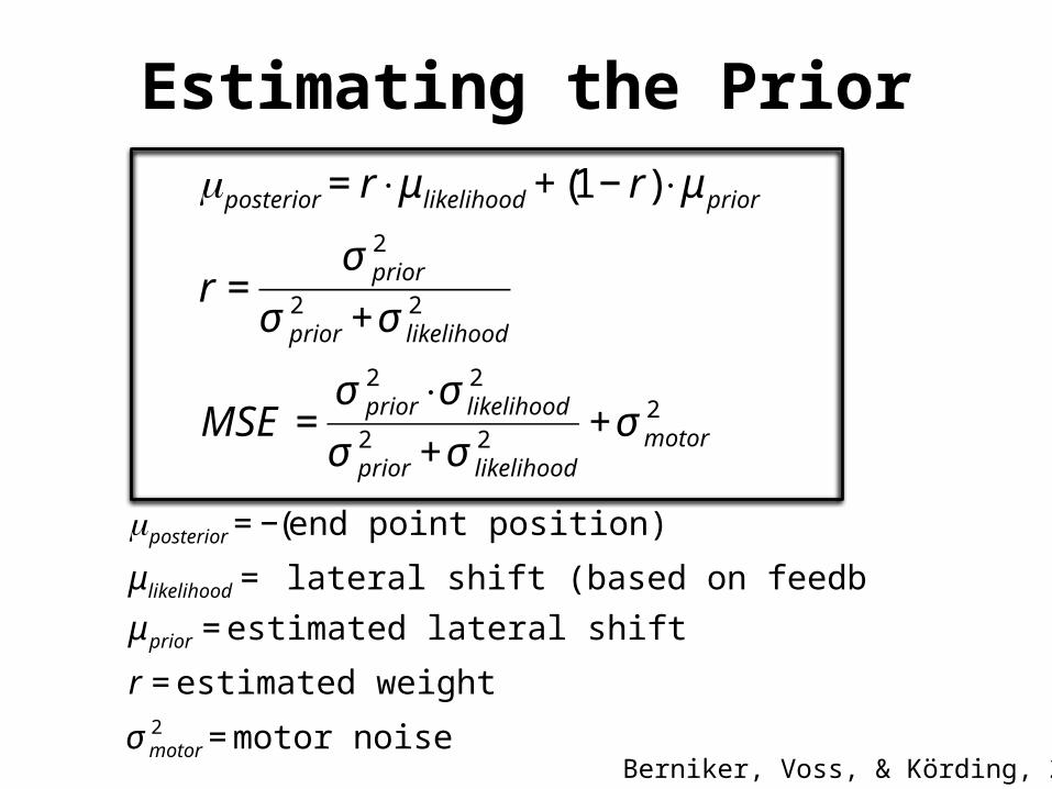
Estimating the Prior
€
μposterior = r⋅ μ likelihood + 1 − r( )⋅ μ prior
r =σ prior
2
σ prior2 +σ likelihood
2
MSE =σ prior
2 ⋅σ likelihood2
σ prior2 +σ likelihood
2 +σ motor2
€
μposterior = −(end point position)
μ likelihood = lateral shift (based on feedback at midpoint)
μ prior = estimated lateral shift
r = estimated weight
σ motor2 = motor noise
Berniker, Voss, & Körding, 2010
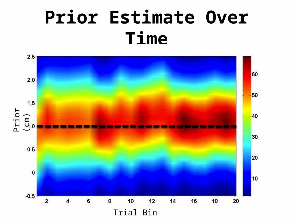
Prior Estimate Over Time
Trial Bin
Pri
or (
cm)

Likelihood Variance
€
σ likelihood2 =
MSE −σ motor2
r
€
μposterior = r⋅ μ likelihood + 1− r( )⋅ μ prior
€
σ likelihood2 : 0.29 0.43 0.60 ∞
σ0 σM σL σ∞

Implementation of Kalman Filter
€
At =α 1 −α1
t −11 −
1
t −1
⎡
⎣ ⎢ ⎢
⎤
⎦ ⎥ ⎥,C = 1 0[ ]
μ =0
0
⎡
⎣ ⎢
⎤
⎦ ⎥,∑ =
1/4 0
0 1/100
⎡
⎣ ⎢
⎤
⎦ ⎥
ε(σ s) =0.36 if cond(σ
s) = 1 ; 0.67 if cond(σ
s) = 2
0.8 if cond(σs
) =3 ; 100 if cond(σs
) =4
⎧ ⎨ ⎪
⎩ ⎪
• Our state vector : Current perturbation Pt and perturbation mean μt computed on all the previous trials
• Our observer: Midpoint Cursor Position
)(
,1
1
smpt
tt
t
tt
t
t
hP
Cy
NP
AP
σμ
μμμ
where:
• Parameter α • Weights the contributions of the previous perturbation and
of the whole history of perturbations in the current prediction
• Is optimized on the training data (first 1000 trials)

Kalman Filter Fit
KalmanFilter
SubjectData
Trial
End
Han
d Po
sitio
n (c
m)
α (across subjects)=0.35
R2 = 0.18
Typical Subject
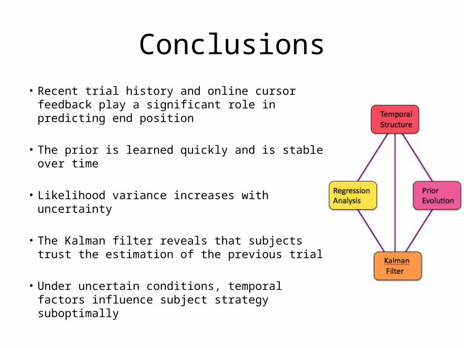
Conclusions• Recent trial history and online cursor
feedback play a significant role in predicting end position
• The prior is learned quickly and is stable over time
• Likelihood variance increases with uncertainty
• The Kalman filter reveals that subjects trust the estimation of the previous trial
• Under uncertain conditions, temporal factors influence subject strategy suboptimally
M I L A D Y


