Temporal Multivariate Networks

James Abello1, Daniel Archambault2, Jessie Kennedy3, Stephen Kobourov4,Kwan Liu Ma5, Silvia Miksch6, Chris Muelder5, and Alexandru Telea7

1 Rutgers University abello@dimacs.rutgers.edu2 Swansea University d.w.archambault@swansea.ac.uk3 Edinburgh Napier University j.kennedy@napier.ac.uk

4 University of Arizona kobourov@cs.arizona.edu5 University of California at Davis {ma, cwmuelder}@ucdavis.edu

6 Vienna University of Technology miksch@ifs.tuwien.ac.at7 University of Groningen a.c.telea@rug.nl

Abstract. Networks that evolve over time, or dynamic graphs, havebeen of interest to the areas of information visualization and graph draw-ing for many years. Typically, its the structure of the dynamic graph thatevolves as vertices and edges are added or removed from the graph. Ina multivariate scenario, however, attributes play an important role andcan also evolve over time. In this chapter, we characterize and surveymethods for visualizing temporal multivariate networks. We also explorefuture applications and directions for this emerging area in the fields ofinformation visualization and graph drawing.

1 Introduction

In previous chapters, this book has primarily concerned itself with visualizationmethods for static, multivariate graphs. In a static scenario, the network has anumber of attributes associated with its elements. These attribute values remainfixed and the challenge is to visualize the interactions between the network(s)and these attributes. Static multivariate graphs could be viewed as graphs withan associated high dimensional data set linked to its elements.

Time is simply another dimension in this multivariate data set that caninteract with the vertices, edges, and attribute values of the network. However,humans perceive time differently as we know from our everyday interactions withthe physical world. Thus, intuitively, this dimension is often handled differentlywhen supporting the presentation of data that changes over time. Visualizationapplications and techniques have, and probably should, continue to exploit thisfact, allowing for effective visualization methods of temporal multivariate graphs.

In this chapter, we define, characterize, and summarize the data and visual-ization techniques relating to temporal multivariate networks. Section 2 providesdefinitions and examples that characterize the networks we address in this chap-ter. We further refine our definitions of time in section 3. In section 4, we surveyrepresentations for dynamic multivariate networks and provide a survey of vi-sualization techniques. We describe the visualization of temporal multivariate

2

networks in the domain of software engineering in section 5. Finally, section 6describes open problems in this area.

2 Definitions

In a variety of applications, time varying multivariate data can be viewed asevolving information networks whose structure is derived from data attributes(i.e. via similarity measures), or it is specified a priory (i.e. the flow of infor-mation over an underlying network), or it is the result of tracking behavioralstatistics (i.e. network traces). The network and attributes can be:

– inherent to the fundamental data elements that are taken to be the networkvertices (name, age, gender, income, profession, interests . . . )

– indicators of the type of relation between the network vertices (professor of,father of, boss of, colleague of . . . )

– attribute derived data (time varying computational mappings from vertexattributes to edge attributes such as “pairs of stocks in markets whose per-formance has been above a given threshold during a time period”)

– structural derived statistics (vertex ranks, network centrality, clustering mea-sures . . . )

– specified contexts in which the data occurs (Tweets related to a given set ofkey words for a specified time period)

In the next subsection, we adapt a model used in software engineering for thepurposes of characterizing the types of dynamic, multivariate networks that canbe visualized. Then, we propose mathematical formalizations of time varyingmultivariate networks.

2.1 Structure, Behavior, and Evolution

In a static multivariate network analysis scenario, we have a network struc-ture, consisting of vertices and edges, as well as attributes associated with thesevertices and edges. In a time varying scenario, both the graph structure andattribute values can evolve over time. In most cases, we can assume that thenetwork structure at a given moment in time can influence how the attributevalues evolve and vice versa. These interactions are in some respects very similarto those considered in some software engineering contexts [28]. Thus, we exam-ine time varying multivariate networks appearing in biology and social networksunder the lenses of structure, behavior and evolution.

– Structure: Pairings between parts or elements of a complex system. Struc-ture mostly relates to the topology of the underlying network at a given timet.

– Behavior: Observable activity. Action or reaction of system elements undera given set of stimuli. Behavior mostly refers to the attributes associatedwith the underlying network elements and how they change over time.

3

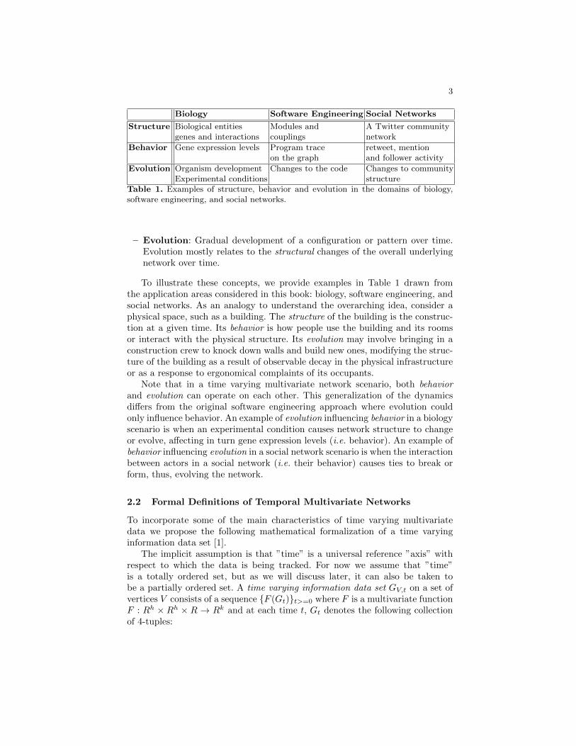
Biology Software Engineering Social Networks

Structure Biological entities Modules and A Twitter communitygenes and interactions couplings network

Behavior Gene expression levels Program trace retweet, mentionon the graph and follower activity

Evolution Organism development Changes to the code Changes to communityExperimental conditions structure

Table 1. Examples of structure, behavior and evolution in the domains of biology,software engineering, and social networks.

– Evolution: Gradual development of a configuration or pattern over time.Evolution mostly relates to the structural changes of the overall underlyingnetwork over time.

To illustrate these concepts, we provide examples in Table 1 drawn fromthe application areas considered in this book: biology, software engineering, andsocial networks. As an analogy to understand the overarching idea, consider aphysical space, such as a building. The structure of the building is the construc-tion at a given time. Its behavior is how people use the building and its roomsor interact with the physical structure. Its evolution may involve bringing in aconstruction crew to knock down walls and build new ones, modifying the struc-ture of the building as a result of observable decay in the physical infrastructureor as a response to ergonomical complaints of its occupants.

Note that in a time varying multivariate network scenario, both behaviorand evolution can operate on each other. This generalization of the dynamicsdiffers from the original software engineering approach where evolution couldonly influence behavior. An example of evolution influencing behavior in a biologyscenario is when an experimental condition causes network structure to changeor evolve, affecting in turn gene expression levels (i.e. behavior). An example ofbehavior influencing evolution in a social network scenario is when the interactionbetween actors in a social network (i.e. their behavior) causes ties to break orform, thus, evolving the network.

2.2 Formal Definitions of Temporal Multivariate Networks

To incorporate some of the main characteristics of time varying multivariatedata we propose the following mathematical formalization of a time varyinginformation data set [1].

The implicit assumption is that ”time” is a universal reference ”axis” withrespect to which the data is being tracked. For now we assume that ”time”is a totally ordered set, but as we will discuss later, it can also be taken tobe a partially ordered set. A time varying information data set GV,t on a set ofvertices V consists of a sequence {F (Gt)}t>=0 where F is a multivariate functionF : Rh × Rh × R → Rk and at each time t, Gt denotes the following collectionof 4-tuples:

4

Gt = {< V(x,y), Vx, Vy, t >: V(x,y) = F (Vx, Vy, t)} (1)

Vx , Vy , and V(x,y) are vectors in Rh and Rk respectively and (x, y) is a pairof vertices in V . The underlying information network structure is determined bythose pairs of vertices (x, y) in V × V for which there exists a four tuple

< V(x,y), Vx, Vy, t >

in some Gt.The F cumulative behavior of GV,t up to and including t is the entry wise

sum:

F<=t(GV ) =<

t∑j=0

(V(x,y)),

t∑j=0

(Vx),

t∑j=0

(Vy) >

where the sum is taken over all the quadruples < V(x,y), Vx, Vy, j > in Gj forj <= t.

A time varying information data set GV,t evolves towards a network G, ifthere exists a time t > 0 such that the underlying network of the union of Gj forj >= t is isomorphic to G.

3 Refining Our Models and Definitions for Time

Time itself is an inherent data dimension that is central to the tasks of revealingtrends and identifying patterns and relationships in the data. Time and time-oriented data have distinct characteristics that make it worthwhile to treat suchdata as a separate data type [2, 3]. Due to the importance of time-oriented data,its structure has been studied in numerous scientific publications (e.g., [2, 11,41]). As proposed by Aigner et al. [3], we divide the aspects of time-orienteddata into general aspects required to adequately model the time domain as wellas hierarchical organization of time and definition of concrete time elements, alsocalled human-made abstractions.

The general aspects are scale, scope, arrangement, and viewpoints.1. Scale: ordinal vs. discrete vs. continuous. As a first perspective, we look at

time from the scale along which elements of the model are given. In an ordinaltime domain, only relative order relations are present (e.g., before, after). Indiscrete domains temporal distances can also be considered. Time values canbe mapped to a set of integers which enables quantitative modelling of timevalues (e.g., quantifiable temporal distances). Discrete time domains are basedon a smallest possible unit and they are the most commonly used time modelin information systems. Continuous time models are characterized by a possiblemapping to real numbers, i.e., between any two points in time, another point intime exists (also known as dense time).

2. Scope: point-based vs. interval-based. Secondly, we consider the scope ofthe basic elements that constitute the structure of the time domain. Point-based

5

time domains can be seen in analogy to discrete Euclidean points in space, i.e.,having a temporal extent equal to zero. Thus, no information is given aboutthe region between two points in time. In contrast to that, interval-based timedomains relate to subsections of time having a temporal extent greater thanzero. This aspect is also closely related to the notion of granularity, which willbe discussed later.

3. Arrangement: linear vs. cyclic. As the third design aspect, we look atthe arrangement of the time domain. Corresponding to our natural perceptionof time, we mostly consider time as proceeding linearly from the past to thefuture, i.e., each time value has a unique predecessor and successor. In a cyclicorganization of time, the domain is composed of a set of recurring time values(e.g., the seasons of the year). Hence, any time value A is preceded and succeededat the same time by any other time value B (e.g., winter comes before summer,but winter also succeeds summer).

4. Viewpoint: ordered vs. branching vs. multiple perspectives. The fourth sub-division is concerned with the views of time that are modelled. Ordered timedomains consider things that happen one after the other. On a more detailedlevel, we might also distinguish between totally ordered and partially ordereddomains. In a totally ordered domain only one thing can happen at a time. Incontrast to this, simultaneous or overlapping events are allowed in partially or-dered domains, i.e., multiple time primitives at a single point or overlapping intime. A more complex form of time domain organization is the so-called branch-ing time. Here, multiple strands of time branch out and allow the descriptionand comparison of alternative scenarios (e.g., in project planning). In contrast tobranching time where only one path through time will actually happen, multipleperspectives facilitate simultaneous (even contrary) views of time.

The human-made abstractions are granularities, time primitives, and de-terminacy.

1. Granularity and calendars: none vs. single vs. multiple. To tackle the com-plexity of time and to provide different levels of granularity, useful abstractionscan be employed. Basically, granularities can be thought of as (human-made)abstractions of time in order to make it easier to deal with time in every-daylife (like minutes, hours, days, weeks, months). More generally, granularities de-scribe mappings from time values to larger or smaller conceptual units. If agranularity and calendar system is supported by the time model, we character-ize it as multiple granularities. Besides this complex variant, there might be asingle granularity only (e.g., every time value is given in terms of milliseconds)or none of these abstractions are supported (e.g., abstract ticks).

2. Time primitives: instant vs. interval vs. span. These time primitives canbe seen as an intermediary layer between data elements and the time domain.Basically, time primitives can be divided into anchored (absolute) and unan-chored (relative) primitives. Instant and interval are primitives that belong tothe first group, i.e., they are located on a fixed position along the time domain.In contrast to that, a span is a relative primitive, i.e., it has no absolute posi-tion in time. Instants are a model for single points in time, intervals for ranges

6

between two points in time, and spans a duration (of intervals) without a fixedposition.

3. Determinacy: determinate vs. indeterminate. Uncertainty is another im-portant aspect when considering time-oriented data. If there is no complete orexact information about time specifications or if time primitives are convertedfrom one granularity to another, uncertainties are introduced and have to bedealt with. Therefore, the determinacy of the given time specification needs tobe considered. A determinate specification is present when there is completeknowledge of all temporal aspects.

4 Survey of Representations and Algorithms

While static graphs arise in many applications, dynamic processes naturally giverise to graphs that evolve through time. Such dynamic processes can be foundin software engineering, telecommunications traffic, computational biology, andsocial networks, among others. Dynamic graph drawing addresses the problemof effectively presenting such relationships as they change over time.

Static graph visualization has a long and venerable history, while dynamicgraph visualization is a relatively newer field. But even though temporal graphrepresentations are more recent, the variety of representations is still large, andthere are a number of studies concerning the drawing of dynamic graphs [20, 5,16]. As a dynamic graph can be thought of as a sequence of edge sets on thesame set of vertices, it can be treated similarly to visualizing multiple relation-ships on the same data set. There are nearly as many ways to represent dynamicor multivariate networks as there are graph representations: simple node-linkdiagrams, directed graphs, clustered graphs, hierarchical and multi-level repre-sentations, matrix representations, spatialized (map-like) representations, etc.Dynamic graphs can be visualized with global views, where all the graphs aredisplayed at once, merged views, where all the graphs are agglomerated together,and with sequenced views, where timesteps are plotted individually, and eithersmall multiples or animated morphing (fading in/out vertices and edges thatappear/disappear) are used to compare timesteps.

It is worth noting here that it makes a difference whether the temporal vi-sualization aims to show individual timesteps (e.g., collaboration between re-searchers in each individual year) or cumulative (e.g., new collaborations fromcurrent year are added to the already accumulated collaboration graph). Simi-larly, there is a difference between offline and online temporal visualization. Inthe offline setting, we are given all data in advance, whereas in the online settingthe changes are happening on the fly. Most existing algorithms address the prob-lem of offline dynamic graph drawing, where the entire sequence of graphs to bedrawn is known in advance. This gives the layout algorithm information aboutfuture changes in the graph, which makes it possible to optimize the layoutsgenerated across the entire sequence (e.g., the algorithm can leave enough spacein anticipation of placing vertices that appear later in the sequence). Less work

7

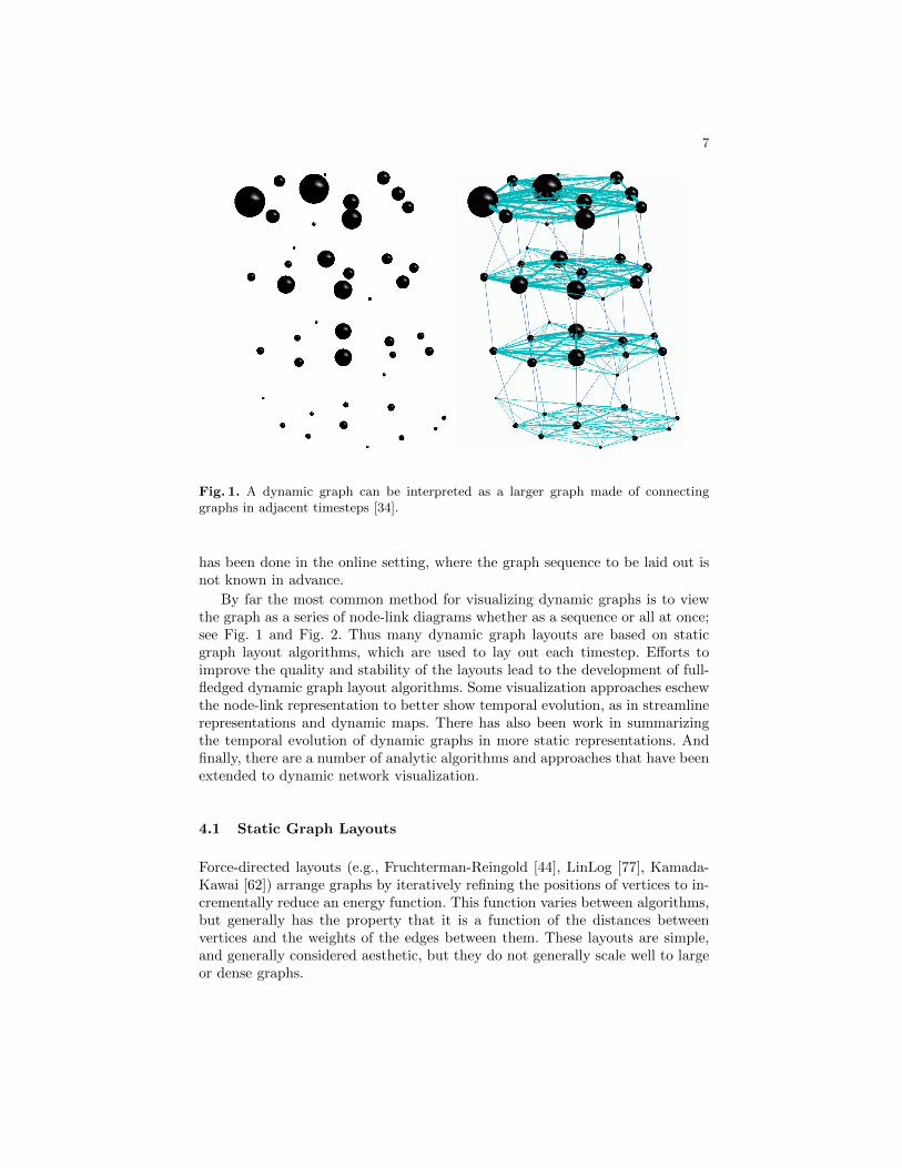
Fig. 1. A dynamic graph can be interpreted as a larger graph made of connectinggraphs in adjacent timesteps [34].

has been done in the online setting, where the graph sequence to be laid out isnot known in advance.

By far the most common method for visualizing dynamic graphs is to viewthe graph as a series of node-link diagrams whether as a sequence or all at once;see Fig. 1 and Fig. 2. Thus many dynamic graph layouts are based on staticgraph layout algorithms, which are used to lay out each timestep. Efforts toimprove the quality and stability of the layouts lead to the development of full-fledged dynamic graph layout algorithms. Some visualization approaches eschewthe node-link representation to better show temporal evolution, as in streamlinerepresentations and dynamic maps. There has also been work in summarizingthe temporal evolution of dynamic graphs in more static representations. Andfinally, there are a number of analytic algorithms and approaches that have beenextended to dynamic network visualization.

4.1 Static Graph Layouts

Force-directed layouts (e.g., Fruchterman-Reingold [44], LinLog [77], Kamada-Kawai [62]) arrange graphs by iteratively refining the positions of vertices to in-crementally reduce an energy function. This function varies between algorithms,but generally has the property that it is a function of the distances betweenvertices and the weights of the edges between them. These layouts are simple,and generally considered aesthetic, but they do not generally scale well to largeor dense graphs.

8

Fig. 2. Snapshots of the call-graph of a program as it evolves through time, extractedfrom CVS logs. Vertices start out red. As time passes and a vertex does not changeit turns purple and finally blue. When another change is affected, the vertex againbecomes red. Note the number of changes between the two large clusters and the breakin the build on the last image [24].

More efficient layout algorithms use a multi-scale approach, such as the workof Cohen [23], the Fast Multipole Multilevel Method (FM3) [52], and the GraphdRawing with Intelligent Placement (GRIP) algorithm [46]. These algorithmsstart by laying out a small approximation of a graph, then progressively layingout finer approximations of the graph, until the entire original graph is laid out.These algorithms generally use far fewer iterations, and thus perform far betterthan traditional force-directed approaches, while still producing similar results.

Even faster graph layout algorithms are available in the form of algebraiclayouts, such as Algebraic Multigrid Computation of Eigenvectors (ACE) [64],High Dimensional Embedding (HDE) [53], the work of Brandes and Pich [18],or the Maxent method [48]. These calculate layouts directly using linear algebratechniques rather than using iterative force calculations. This generally makesthem very fast. Clustering-based layouts have also been shown to be fast, asin the case of the treemap layout [74] or space-filling curve layout [73]. Thesemethods work by clustering the graph in a preprocessing step and then mappingthe clustering to the screen to define the layout itself.

4.2 Dynamic Graph Layouts

In dynamic graph drawing the goal is to maintain a nice layout of a graph that ismodified via operations such as inserting/deleting edges and inserting/deletingvertices. A key property of in many real-world applications, where dynamicgraphs naturally arise, is that the difference between any two timesteps is gen-erally assumed to be incremental: that is, a small change relative to the size ofthe graph. If the change between timesteps is too large, then it is often moreeffective to treat them as separate, static networks. When visualizing evolvingand dynamic graphs, two of the most important criteria to consider are:

1. readability, or quality of the individual layouts, which depends on aestheticcriteria such as display of symmetries, uniform edge lengths, and minimalnumber of crossings; and

9

Fig. 3. Mental map preservation has been a forefront topic in dynamic graph layout.The level of layout stability can vary between approaches. Incremental approaches canrange from having no correlation between timesteps to using the previous timestep asinitialization to anchoring or tethering some vertices to previous positions. The moststable layouts agglomerate all timesteps together, but these could result in poor layoutsat each timestep.

2. mental map preservation, or stability in the series of layouts, which can beachieved by ensuring that vertices and edges that appear in consecutivegraphs in the series, remain in the same location.

There is an inherent trade-off between the stability and quality of any dynamicgraph layout, as restricting the movement of vertices could make it impossible toachieve high quality layout of the individual timesteps. In fact, these two criteriaare often contradictory and many dynamic graph layout approaches exploredifferent ways of balancing stability and quality; see Fig. 3. At one end arequality optimizing layouts with little to no correlation between timesteps, andat the other are fixed layouts where the vertices never move, even if the layoutis not ideal for any given timestep. Anchored layouts lie somewhere between thetwo extremes, where some vertices are fixed while others are allowed to move;see survey of Brandes et al. [16].

The input to this problem is a series of graphs defined on the same underlyingset of vertices. As a consequence, nearly all existing approaches to visualizationof evolving and dynamic graphs are based on extensions of static graph layouts,usually based on a force-directed method. The simplest methods just initialize aforce directed layout with the previous layout of the timestep, as in [10, 37], butthis offers little guarantees for stability as nothing actually constrains the motionof vertices. Early examples of this can be dated back to North’s DynaDAG [78],where the graph is not given all at once, but incrementally. Most of these earlyapproaches, however, are limited to special classes of graphs and usually do not

10

scale to graphs over a few hundred vertices. TGRIP could handle the larger graphsthat appear in the real-world. It was developed as part of a system that keepstrack of the evolution of software by extracting information about the programstored within a CVS version control system [24]. Such tools allow programmers tounderstand the evolution of a legacy program: Why is the program structured theway it is? Which programmers were responsible for which parts of the programduring which time periods? Which parts of the program appear unstable overlong periods of time? TGRIP was used to visualize inheritance graphs, programcall-graphs, and control-flow graphs, as they evolve over time; see Fig. 2.

Aggregate layouts such as in [70], are among the approaches that guaranteegood stability by computing one layout for an aggregate graph made up of theunion of all timesteps. Brandes and Corman [14] describe a system for visualizingnetwork evolution in which both fixes vertices in constant locations, and uses a3D super-graph, by showing each modification in a separate layer of a 3D repre-sentation with vertices common to two layers represented as columns connectingthe layers. Thus, mental map preservation is achieved by pre-computing good lo-cations for the vertices and fixing the position throughout the layers. An explicittradeoff between quality and stability can also be provided as in the GraphAELsystem [35]. There a super-graph of all timesteps is created and links betweenoccurrences of the vertices in neighboring timesteps are added; see Fig. 1. Bychanging the weights of these inter-timestep edges one can emphasize stabil-ity (make inter-timestep edges very strong) or readability (make inter-timestepedges very weak). Such approaches [35, 36, 32, 39] generally use modified versionsof traditional static layout algorithms directly, but often induce high memoryusage and complexity because all timesteps are loaded at once. They are alsoonly applicable to offline graph drawing, as the entire data range is needed atthe beginning.

However, the most popular approach in recent years is to compute timevarying network layouts by adding additional constraints that anchor verticesto their positions in the previous timestep [67, 42, 43]. These techniques work byadding some additional forces to the force direction calculation, but provide agood balance of cost, layout quality, and stability, and can be tuned by adjustingthe anchor weights. These algorithms can also address the online dynamic graphdrawing problem, as it is not necessary that the graph sequence is not knownin advance. Brandes and Wagner adapt the force-directed model to dynamicgraphs using a Bayesian framework [19]. An algorithm for visualizing dynamicsocial networks is discussed in [70]. Frishman and Tal consider dynamic drawingof clustered graphs [42] and of general graphs [43]. Brandes et al. have alsoperformed a quantitative evaluation of the tradeoffs between layout quality andstability for these different classes of layouts [17].

There are also dynamic graph visualization approaches based on clustering.Kumar and Garland describe a method of animating clusters through time [65].In this approach, a stratified, abstracted version of the graph is used, where thevertices are topologically sorted into a treelike structure (before layout) in orderto expose interesting features.

11

Sallaberry et al. [94] cluster every timestep individually, associate the clustersacross time, and use the space-filling curve approach to render each timestep; seeFig. 4. Pre-computing the clusters is computationally expensive. Hu et al. [58]propose a method based on a geographical metaphor to visualize a summary ofclustered dynamic graphs. It also relies on clustering and aims to keep clustersstable over time.

(a) 2002-10-27 (b) 2005-09-18 (c) 2009-08-02

Fig. 4. Large networks add additional challenges in computational cost and perceptuallimits (images from [94])

4.3 Animation Versus Small Multiples

Often, dynamic graph visualizations animate the transitions between node-linkdiagrams of timesteps [78, 29, 35, 49, 13, 43]. In these animations, vertices dynam-ically appear, disappear and move to produce readable layouts at each timestep.Diehl and Gorg [29] and Gorg et al. [49] consider graphs in a sequence to createsmoother transitions. Animations as a means to convey an evolving underlyinggraph have also been used in the context of software evolution [24] and scientificliterature visualization [35]. Creating smooth animation between changing se-quences of graphs is addressed using spectral graph visualization in [15]. Whenusing the animation/morphing approach, it is possible to change the balance be-tween readability of individual graphs and the overall mental map preservation,as in the system for Graph Animations with Evolving Layouts, GraphAEL [35,40]. Applications of this framework include visualizing software evolution [24],social networks analysis [9], and the behavior of dynamically modifiable code [30].

Robertson et al. [89] evaluate the effectiveness of three trend visualizationtechniques. The results indicate that animation, often enjoyable and exciting,is not always well suited to data analysis. The other common alternative forvisualizing multiple timesteps is to statically place them next to each other assmall multiples [101]. This eases the comparison of distant timesteps but only asmall area can be devoted to each timestep, which reduces the readability of eachgraph. Cerebral [8] is a system that uses a biologically guided graph layout and

12

incorporates experimental data directly into the graph display. Small multipleviews of different experimental conditions and a data-driven parallel coordinatesview enable correlations between experimental conditions to be analyzed at thesame time that the data is viewed in the graph context. This combination ofcoordinated views allows the biologist to view the data from many differentperspectives simultaneously.

Empirical studies to compare the advantages and drawbacks of these ap-proaches (“Animation” vs. “Small Multiples”) have been performed by Archam-bault et al. [7] as well as Farrugia and Quigley [38]. And even more recently,Rufiange et al. have developed a hybrid approach that lets the user interactivelycombine or switch between animations, small multiples, and plots that explicitlyindicate what has changed [90].

4.4 Mental Map Preservation

Preserving the mental map, or layout stability, is a major focus in many dy-namic node-link representations approaches [17, 43, 58, 65, 92]. Even though sev-eral experiments have been performed to examine the effect of preserving themental map in dynamic graphs visualization the results are mixed. The resultsof [87] were quite surprising. The experiment found that the most effective vi-sualizations were the extreme ones, i.e., the ones with very low or high mentalmap preservation, while visualizations with medium preservation were less effec-tive [87]. With large networks, stability becomes even more important, but sodoes “motion coherency”. Even small motions on each vertex are too much toperceive if they are chaotic, but if vertices move coherently, they can be perceivedas a single group [94]. In a series of papers Archambault and Purchase evaluatevarious approaches for dynamic graph visualization and consider how they affectmental map preservation [7, 4, 6], also summarized in a recent survey [5].

4.5 Alternative Representations

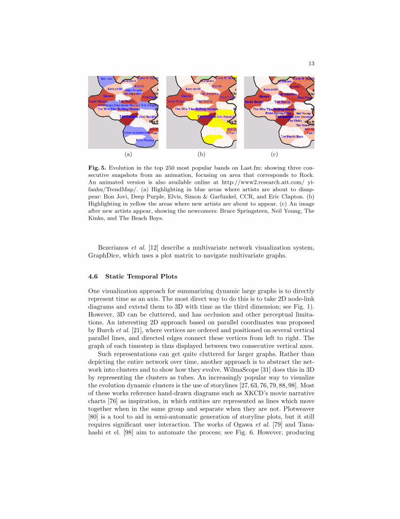
Using maps to visualize non-cartographic data has been considered in the contextof spatialization [97]. Map-like visualization using layers and terrains to representtext document corpora dates back to 1995 [103]. The problem of effectivelyconveying change over time using a map-based visualization was studied byHarrower [54]. More recently, Mashima et al. [68] use the GMap framework [57]to visualize dynamic graphs with the geographic map metaphor; see Fig. 5.

Also related is work on visualizing subsets of a set of items. Areas of inter-est in a UML diagram can be highlighted using a deformed convex hull [22].Isocontours-based bubblesets can be used to depict multiple relations definedon a set of items [25]. Automatic Euler diagrams, which show the grouping ofsubsets of items by drawing contiguous regions around them have also been con-sidered [96]. Apart from differences in the algorithms used to generate regions,all of these approaches create regions that overlap with each other (unlike thestrict map metaphor where regions do not overlap).

13

(a) (b) (c)

Fig. 5. Evolution in the top 250 most popular bands on Last.fm: showing three con-secutive snapshots from an animation, focusing on area that corresponds to Rock.An animated version is also available online at http://www2.research.att.com/ yi-fanhu/TrendMap/. (a) Highlighting in blue areas where artists are about to disap-pear: Bon Jovi, Deep Purple, Elvis, Simon & Garfunkel, CCR, and Eric Clapton. (b)Highlighting in yellow the areas where new artists are about to appear. (c) An imageafter new artists appear, showing the newcomers: Bruce Springsteen, Neil Young, TheKinks, and The Beach Boys.

Bezerianos et al. [12] describe a multivariate network visualization system,GraphDice, which uses a plot matrix to navigate multivariate graphs.

4.6 Static Temporal Plots

One visualization approach for summarizing dynamic large graphs is to directlyrepresent time as an axis. The most direct way to do this is to take 2D node-linkdiagrams and extend them to 3D with time as the third dimension; see Fig. 1).However, 3D can be cluttered, and has occlusion and other perceptual limita-tions. An interesting 2D approach based on parallel coordinates was proposedby Burch et al. [21], where vertices are ordered and positioned on several verticalparallel lines, and directed edges connect these vertices from left to right. Thegraph of each timestep is thus displayed between two consecutive vertical axes.

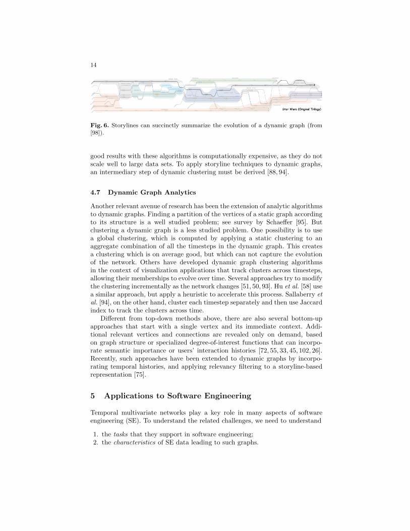
Such representations can get quite cluttered for larger graphs. Rather thandepicting the entire network over time, another approach is to abstract the net-work into clusters and to show how they evolve. WilmaScope [31] does this in 3Dby representing the clusters as tubes. An increasingly popular way to visualizethe evolution dynamic clusters is the use of storylines [27, 63, 76, 79, 88, 98]. Mostof these works reference hand-drawn diagrams such as XKCD’s movie narrativecharts [76] as inspiration, in which entities are represented as lines which movetogether when in the same group and separate when they are not. Plotweaver[80] is a tool to aid in semi-automatic generation of storyline plots, but it stillrequires significant user interaction. The works of Ogawa et al. [79] and Tana-hashi et el. [98] aim to automate the process; see Fig. 6. However, producing

14

Fig. 6. Storylines can succinctly summarize the evolution of a dynamic graph (from[98]).

good results with these algorithms is computationally expensive, as they do notscale well to large data sets. To apply storyline techniques to dynamic graphs,an intermediary step of dynamic clustering must be derived [88, 94].

4.7 Dynamic Graph Analytics

Another relevant avenue of research has been the extension of analytic algorithmsto dynamic graphs. Finding a partition of the vertices of a static graph accordingto its structure is a well studied problem; see survey by Schaeffer [95]. Butclustering a dynamic graph is a less studied problem. One possibility is to usea global clustering, which is computed by applying a static clustering to anaggregate combination of all the timesteps in the dynamic graph. This createsa clustering which is on average good, but which can not capture the evolutionof the network. Others have developed dynamic graph clustering algorithmsin the context of visualization applications that track clusters across timesteps,allowing their memberships to evolve over time. Several approaches try to modifythe clustering incrementally as the network changes [51, 50, 93]. Hu et al. [58] usea similar approach, but apply a heuristic to accelerate this process. Sallaberry etal. [94], on the other hand, cluster each timestep separately and then use Jaccardindex to track the clusters across time.

Different from top-down methods above, there are also several bottom-upapproaches that start with a single vertex and its immediate context. Addi-tional relevant vertices and connections are revealed only on demand, basedon graph structure or specialized degree-of-interest functions that can incorpo-rate semantic importance or users’ interaction histories [72, 55, 33, 45, 102, 26].Recently, such approaches have been extended to dynamic graphs by incorpo-rating temporal histories, and applying relevancy filtering to a storyline-basedrepresentation [75].

5 Applications to Software Engineering

Temporal multivariate networks play a key role in many aspects of softwareengineering (SE). To understand the related challenges, we need to understand

1. the tasks that they support in software engineering;2. the characteristics of SE data leading to such graphs.

15

This section covers the above two points. For a full overview of applicationsof multivariate dynamic graphs in SE, we refer to Chapter ??. Our focus here ismore technical. Specifically, we aim to characterize SE graphs from the perspec-tive of time modeling (Section 3), and the variability axes (of types) (Section 4).This in turn better explains the rationale behind the visual designs presentedin Chapter ??, and also why it is challenging to use visualization techniquesdeveloped for other types of temporal multivariate graphs to handle SE graphs.

Tasks Software engineering activities cover the entire software product lifetime,starting with requirement gathering, followed by architecting, design, implemen-tation (coding), testing, release, and ending with maintenance. Graphs are cre-ated and used in all these stages, as shown in Table 2. As software systems changeduring their lifecycle, all above graphs are by nature time-dependent. Moreover,SE graphs involve elements and relations spanning several of the above activities.For example, in reverse engineering, we encounter graphs that link software testresults with source code (and developers), class diagrams, and requirements.

Actions Examples of graphs

Requirements Requirements vs tasks vs stakeholders[60]UML use-case diagrams[91]

Architecting System structure (layering, dataflows, component interactions)[100]

UML component and package diagrams[91]Design UML class, activity diagrams[91]

Coding Call, inheritance, type-use, and include graphs[28]

Testing Type-instance graphs, control flow graphs[85]Resource allocation graphs[71].

Release Deployment graphs[81], UML deployment diagrams[91]

Maintenance Developer networks, code duplication graphs[69]Table 2. Examples of multivariate temporal graphs in SE.

Data characteristics Temporal multivariate SE graphs have several charac-teristics which make their computation, efficient manipulation, and above allunderstanding very challenging. Below we outline the main such aspects.

Size: Depending on their type, SE graphs range from a few tens of elements(UML diagrams and developer networks) to hundreds of thousands (call graphs)or even millions of elements (control-flow graphs of large programs). The staticcall graph of the Mozilla Firefox browser (a medium-sized system as compared tolarge telecom or banking software) has, for example, over 500K edges [56]. Cer-tain topology constraints exist for some graphs, e.g. class hierarchies are, usually,trees, and architecture dependencies form a directed acyclic graph. However, inthe general case, little can be said about the global properties of SE graphs.

16

For instance, a call graph can be cyclic (or not), and can have a widely varyingdistribution of number of edges per vertex depending on application type.

Attributes: Each vertex and edge in a SE graph typically has several attributes.These describe both static and dynamic properties of the entity encoded by thatvertex or edge. For instance, annotated semantic graphs (ASGs) for C++ pro-grams have tens of such attributes [99]. Computing software quality metricseasily adds tens of other metrics [66]. Attribute types span a wide spectrum:numerical, categorical, text, and binary. Attribute types are key to effective pro-gram understanding. For instance, the C++ ASG in [99] contains around twohundred different vertex-attribute types that encode the different properties ofthe annotated C++ grammar. Being able to visually distinguish between differ-ent types is essential, e.g. for detecting the presence of specific design or executionpatterns. Missing values are possible e.g. due to limitations of program analysistools or due to incomplete program coverage for execution monitoring tools.

Dynamics: Graphs describing human aspects, such as developer activity, changeslowly, given the continuous nature of software evolution [69]. However, other SEgraphs exhibit different dynamics. For instance, in program execution graphs,large changes can occur in short time periods and few changes in other longertime periods. Dynamics is present both at the structure level (e.g. changes of acall graph topology as the program is run for different inputs or as code changesduring maintenance), and also at the attribute level (e.g. different runtime met-rics measured at static component level for different program executions).

Time modeling: Time is, formally, modeled as a discrete quantity, since bothexecution and changes of software code occur at discrete, moments. Time hasa linear nature, describing the order of execution of program instructions orthe order of changes in a repository. However, time can be seen as fully or-dered or branching (Section 2). The branching case occurs e.g. when consideringexecution of multi-threaded programs or analyzing development activity of arepository with multiple branches. Both point-based and interval-based modelsare used, often interchangeaby, for the same analysis. For instance, a version ina software repository can refer to the moment when it was committed, but alsoto the time interval between this commit time and the next change of the sameartifact.

Scale: Software understanding occurs on multiple levels of detail and followingboth a top-down and bottom-up process [85]. Hence, one needs to (visually)analyze software at several levels of detail or scales. SE graphs offer severalnatural scales, given their hierarchical, or compound, nature (Chapter ??), e.g.function-class-file-folder or the structure given by a function call stack. Yet,several aspects make constructing efficient and effective multiscale SE-graphvisualizations hard. Firstly, SE graphs are huge. The few above-mentioned levelsof detail do not offer enough granularity to automatically simplify large graphs to

17

levels where they can be displayed in an understandable manner. Automaticallycomputing additional levels of detail is hard – for instance, what should be themeaning of an artifact larger than a file, but smaller than a folder? Secondly,many program understanding tasks require showing both fine-grained detail andcoarse-scale structure in the same view. For instance, to debug a crash, we needto see the entire call stack, from the finest-grained instruction which caused thefault up to the coarse-level components which scope the fault. Finally, softwareis by nature abstract. As such, finding effective visual metaphors (for both thespatial graph embedding and attribute mapping) is challenging.

6 Open Problems

Although significant progress has been achieved in the design of visualizationmethods and tools for exploring multivariate temporal networks, several impor-tant open challenges remain. This section outlines a selection of challenges whichare relevant to a broad subset of applications involving such graphs. Throughoutthe discussion, we use the notation introduced in Section 2.2.

6.1 Attribute dimensionality

As outlined in Section 5, SE graphs are high-variate, i.e., have many attributesfor each vertex or edge. Existing visualization techniques can simultaneouslyshow a few (up to 3) attributes per graph element, by mapping these to shape,size, texture, color, and shading. However, this solution scales poorly for graphsof hundreds of thousands of elements. Separately, even for small graphs (hun-dreds of elements), showing tens of attributes per element is an open challenge.Parallel coordinate plots partially address this quest [59]. An interesting adap-tion hereof clusters graph vertices based on attribute values, and links the re-sulting icicle plots to a table-lens-like visualization of the edge attributes, tohighlight attribute correlations [86]. Dimensionality reduction projects a set ofhigh-dimensional attributes into R2 or R3 so that similarities between the origi-nal attributes are reflected in the low-dimensional distance [61, 82, 83]. Althoughsuch approaches scale well computationally for large sample counts [84], it is hardto visualize both attribute similarity and graph structure in the same embedding.Other approaches use interactive brushing, attribute selection, and linked views.However, none of the above methods fully enables users to correlate structurewith attributes, and attributes among themselves, for highly-variate graphs.

6.2 Capturing patterns

In many use-cases, showing a picture of the (changing) graph is not sufficient,even when this picture is clutter and overlap-free. For instance, consider the taskof locating patterns in the graph. Patterns are specific configurations of verticesand edges (topology) and attribute values which capture events of interest. Pat-terns are typically problem-dependent, and have a certain variability in both

18

structure and attribute values. Consider finding a ‘multithreading refactoringevent’ in a software code base: This would involve finding similar code frag-ments in a graph Gt, which describe serial code, and finding that they have beenreplaced by functionally-identical multithreaded code in the following revisionGt+1 of the code base. Even the simpler ‘design patterns’ [47], well known andused in object-oriented software design, are hard to detect and visualize. Theunderlying reasons are twofold. First, patterns involve, by definition, severalvertices, edges, and attribute values, so they correspond to portions of a graphvisualizations. However, existing graph visualization techniques have difficultiesin showing such data subsets in canonical ways, i.e., in ways that make their vi-sual detection easy. Secondly, patterns have a certain variability. Besides makingautomatic detection hard, this also implies that their graph visualizations willexhibit a necessary variability, which makes their visual detection hard. Finally,visually detecting dynamic patterns is very challenging – if animation is used,this poses high demands on the user’s visual memory; if static visualizations areused, inherently dynamic patterns may be hard to grasp.

6.3 Data size

Large dynamic graphs involve large sets of vertices and edges and/or manysampling moments when the graph is captured. This implies many sample pointstaken over the domain of function F (Equation 1). Large graphs are hard toembed in a low-dimensional space (R2 or R3) so that the graph structure iseasy to discern. This basic graph-drawing problem becomes one or two ordersof magnitude larger for dynamic graphs. The data size problem becomes evenlarger for high-variate graphs.

It is insightful to consider how data size relates to the other challenges. For-mally, we could argue that dynamic multivariate graphs (and their patterns) canbe efficiently and effectively depicted using existing visualization methods, forsmall graphs. Hence, we could use subsampling, like in scientific data visualiza-tion, to reduce the graph size prior to visual exploration. To preserve features orpatterns of interest, data-adaptive subsampling could be used. The main obsta-cle here is that we still lack a comprehensive theory for subsampling graphs andcategorical attributes. As such, existing solutions addressing data size currentlyhave to rely on aggregation and simplification algorithms and heuristics that areproblem, scale, and even dataset-specific.

7 Summary and Conclusions

In this chapter, we characterized temporal multivariate graphs in terms of struc-ture and time. We presented common terminology for discussing temporal multi-variate graphs, a survey of existing techniques, focusing on software engineeringapplications, and a collection of open problems. We hope that this common ter-minology, data characterization, and organization of existing and future workwill help foster further research in the emerging area of dynamic multivariategraph visualization.

19

References

1. J. Abello, S. Hadlak, H. Schumann, and H. Schulz. A modular degree-of-interestspecification for the visual analysis of large dynamic networks. IEEE Transactionson Visualization and Computer Graphics, 2014. in press.

2. W. Aigner, S. Miksch, H. Schumann, and C. Tominski. Visualization of Time-Oriented Data. Springer, London, 2011.

3. N. Andrienko and G. Andrienko. Exploratory Analysis of Spatial and TemporalData: A Systematic Approach. Springer, Berlin, 2006.

4. D. Archambault and H. C. Purchase. The mental map and memorability indynamic graphs. In H. Hauser, S. G. Kobourov, and H. Qu, editors, Proc. of theIEEE Pacific Visualization Symposium, pages 89–96. IEEE, 2012.

5. D. Archambault and H. C. Purchase. The “map” in the mental map: Experimentalresults in dynamic graph drawing. International Journal of Human-ComputerStudies, 71(11):1044 – 1055, 2013.

6. D. Archambault and H. C. Purchase. Mental map preservation helps user orien-tation in dynamic graphs. In Graph Drawing (GD’12), volume 7704 of LNCS,pages 475–486, 2013.

7. D. Archambault, H. C. Purchase, and B. Pinaud. Animation, small multiples,and the effect of mental map preservation in dynamic graphs. IEEE Transactionson Visualization and Computer Graphics, 17(4):539–552, 2011.

8. A. Barsky, T. Munzner, J. Gardy, and R. Kincaid. Cerebral: Visualizing multipleexperimental conditions on a graph with biological context. IEEE Transactionson Visualization and Computer Graphics, 14(6):1253–1260, 2008.

9. M. Bastian, S. Heymann, and M. Jacomy. Gephi: an open source software for ex-ploring and manipulating networks. International AAAI Conference on Weblogsand Social Media, pages 361–362, 2009.

10. S. Bender-deMoll and D. A. McFarland. The art and science of dynamic networkvisualization. Journal of Social Structure, 7(2), 2006.

11. C. Bettini, S. Jajodia, and S. X. Wang. Time Granularities in Databases, DataMining, and Temporal Reasoning. Springer, Berlin, 2000.

12. A. Bezerianos, F. Chevalier, P. Dragicevic, N. Elmqvist, and J.-D. Fekete.Graphdice: A system for exploring multivariate social networks. Computer Graph-ics Forum, 29(3):863–872, 2010.

13. K. Boitmanis, U. Brandes, and C. Pich. Visualizing internet evolution on theautonomous systems level. In Graph Drawing (GD’07), volume 4875 of LNCS,pages 365–376. Springer, 2008.

14. U. Brandes and S. R. Corman. Visual unrolling of network evolution and theanalysis of dynamic discourse. In Proc. of the IEEE Symposium on InformationVisualization, pages 145–151, 2002.

15. U. Brandes, D. Fleischer, and T. Puppe. Dynamic spectral layout with an appli-cation to small worlds. Journal of Graph Algorithms and Applications, 11(2):325–343, 2007.

16. U. Brandes, N. Indlekofer, and M. Mader. Visualization methods for longitudinalsocial networks and stochastic actor-oriented modeling. Social Networks, pages291–308, June 2011.

17. U. Brandes and M. Mader. A quantitative comparison of stress-minimizationapproaches for offline dynamic graph drawing. In Graph Drawing (GD’11), volume7034 of LNCS, pages 99–110. Springer, 2012.

20

18. U. Brandes and C. Pich. An experimental study on distance-based graph drawing.In Graph Drawing, pages 218–229, 2008.

19. U. Brandes and D. Wagner. A Bayesian paradigm for dynamic graph layout. InGraph Drawing (GD’97), pages 236–247, 1998.

20. J. Branke. Dynamic graph drawing. In M. Kaufmann and D. Wagner, editors,Drawing Graphs, volume 2025 of Lecture Notes in Computer Science, pages 228–246. Springer, 2001.

21. M. Burch, C. Vehlow, F. Beck, S. Diehl, and D. Weiskopf. Parallel edge splattingfor scalable dynamic graph visualization. IEEE Transactions on Visualizationand Computer Graphics, 17(12):2344–2353, 2011.

22. H. Byelas and A. Telea. Visualization of areas of interest in software architecturediagrams. In ACM SoftVis’06, pages 105–114, 2006.

23. J. D. Cohen. Drawing graphs to convey proximity: An incremental arrange-ment method. ACM Transactions On Computer-Human Interaction, 4(3):197–229, 1997.

24. C. Collberg, S. G. Kobourov, J. Nagra, J. Pitts, and K. Wampler. A system forgraph-based visualization of the evolution of software. In ACM SoftVis’03, pages77–86, 2003.

25. C. Collins, G. Penn, and S. Carpendale. Bubble sets: Revealing set relations withisocontours over existing visualizations. IEEE Transactions on Visualization andComputer Graphics, 15(6):1009–1016, 2009.

26. T. Crnovrsanin, I. Liao, Y. Wuy, and K.-L. Ma. Visual recommendations fornetwork navigation. In Proc. of the 13th Eurographics / IEEE - VGTC confer-ence on Visualization, EuroVis’11, pages 1081–1090, Aire-la-Ville, Switzerland,Switzerland, 2011. Eurographics Association.

27. W. Cui, S. Liu, L. Tan, C. Shi, Y. Song, Z. Gao, H. Qu, and X. Tong. Textflow:Towards better understanding of evolving topics in text. IEEE Transactions onVisualization and Computer Graphics, 17(12):2412–2421, 2011.

28. S. Diehl. Software Visualization: Visualizing the Structure, Behaviour, and Evo-lution of Software. Springer, Berlin, 2010.

29. S. Diehl and C. Gorg. Graphs, they are changing. In Graph Drawing (GD’02),volume 2528 of LNCS, pages 23–30. Springer, 2003.

30. B. Dux, A. Iyer, S. K. Debray, D. Forrester, and S. G. Kobourov. Visualizing thebehavior of dynamically modifiable code. In IWPC, pages 337–340, 2005.

31. T. Dwyer. Extending the wilmascope 3d graph visualisation system — softwaredemonstration. In S.-H. Hong, editor, APVIS, volume 45 of CRPIT, pages 39–45.Australian Computer Society, 2005.

32. T. Dwyer and D. R. Gallagher. Visualising changes in fund manager holdings intwo and a half-dimensions. Information Visualization, 3:227–244, 2004.

33. N. Elmqvist and J.-D. Fekete. Hierarchical Aggregation for Information Visu-alization: Overview, Techniques, and Design Guidelines. IEEE Transactions onVisualization and Computer Graphics, 16(3):439–454, 2009.

34. C. Erten, P. J. Harding, S. G. Kobourov, K. Wampler, and G. Yee. Exploring thecomputing literature using temporal graph visualization. In Electronic Imaging2004, pages 45–56, 2004.

35. C. Erten, P. J. Harding, S. G. Kobourov, K. Wampler, and G. V. Yee. GraphAEL:Graph animations with evolving layouts. In Graph Drawing (GD’03), volume 2912of LNCS, pages 98–110. Springer, 2004.

36. C. Erten, S. Kobourov, V. Le, and A. Navabi. Simultaneous graph drawing:layout algorithms and visualization schemes. Journal of Graph Algorithms andApplications, 9(1):165–182, 2005.

21

37. M. Farrugia and A. Quigley. Cell phone mini challenge: Node-link animationaward animating multivariate dynamic social networks. In IEEE Visual AnalyticsScience and Technology, pages 215 –216, oct. 2008.

38. M. Farrugia and A. Quigley. Effective temporal graph layout: A comparativestudy of animation versus static display methods. Journal of Information Visu-alization, 10(1):47–64, 2011.

39. K.-C. Feng, C. Wang, H.-W. Shen, and T.-Y. Lee. Coherent time-varying graphdrawing with multi-focus+context interaction. IEEE Transactions on Visualiza-tion and Computer Graphics, 2011.

40. D. Forrester, S. G. Kobourov, A. Navabi, K. Wampler, and G. V. Yee. Graphael:A system for generalized force-directed layouts. In Graph Drawing (GD’03), pages454–464, 2004.

41. A. U. Frank. Different Types of “Times” in GIS. In M. J. Egenhofer and R. G.Golledge, editors, Spatial and Temporal Reasoning in Geographic Information Sys-tems, pages 40–62. Oxford University Press, New York, NY, USA, 1998.

42. Y. Frishman and A. Tal. Dynamic drawing of clustered graphs. In Proc. of theIEEE Symposium on Information Visualization, pages 191–198, Washington, DC,USA, 2004. IEEE Computer Society.

43. Y. Frishman and A. Tal. Online dynamic graph drawing. IEEE Transactions onVisualization and Computer Graphics, 14:727–740, 2008.

44. T. M. J. Fruchterman and E. M. Reingold. Graph drawing by force-directedplacement. Software - Practice and Experience, 21(11):1129–1164, 1991.

45. G. W. Furnas. Generalized fisheye views. In Human Factors in Computing Sys-tems CHI, pages 16–23, 1986.

46. P. Gajer and S. G. Kobourov. GRIP: Graph drawing with intelligent placement.In Graph Drawing (GD’00), pages 222–228, London, UK, 2001. Springer-Verlag.

47. E. Gamma, R. Helm, R. Johnson, and J. Vlissides. Design Patterns: Elements ofReusable Object-Oriented Software. Addison-Wesley, 1994.

48. E. R. Gansner, Y. Hu, and S. C. North. A maxent-stress model for graph layout.In Proc. of the IEEE Pacific Visualization Symposium, pages 73–80, 2012.

49. C. Gorg, P. Birke, M. Pohl, and S. Diehl. Dynamic graph drawing of sequencesof orthogonal and hierarchical graphs. In Graph Drawing (GD’04), volume 3383of LNCS, pages 228–238. Springer, 2005.

50. R. Gorke, P. Maillard, C. Staudt, and D. Wagner. Modularity-driven clusteringof dynamic graphs. In Proc. of the 9th international conference on ExperimentalAlgorithms, SEA’10, pages 436–448, Berlin, Heidelberg, 2010. Springer-Verlag.

51. R. Grke, T. Hartmann, and D. Wagner. Dynamic graph clustering usingminimum-cut trees. In F. Dehne, M. Gavrilova, J.-R. Sack, and C. Tth, edi-tors, Algorithms and Data Structures, volume 5664 of Lecture Notes in ComputerScience, pages 339–350. Springer Berlin Heidelberg, 2009.

52. S. Hachul. A Potential-Field-Based Multilevel Algorithm for Drawing LargeGraphs. PhD thesis, Universitaet zu Koeln, 2002.

53. D. Harel and Y. Koren. Graph drawing by high-dimensional embedding. In GraphDrawing (GD’02), pages 207–219. Springer-Verlag, 2003.

54. M. Harrower. Tips for designing effective animated maps. Cartographic Perspec-tives, 44:63–65, 2003.

55. J. Heer and D. Boyd. Vizster: visualizing online social networks. In Proc. of theIEEE Symposium on Information Visualization, pages 32–39, 2005.

56. H. Hoogendorp, O. Ersoy, D. Reniers, and A. Telea. Extraction and visualizationof call dependencies for large C/C++ code bases: A comparative study. In Proc.ACM VISSOFT, pages 137–145, 2009.

22

57. Y. Hu, E. R. Gansner, and S. G. Kobourov. Visualizing graphs and clusters asmaps. IEEE Computer Graphics and Applications, 30(6):54–66, 2010.

58. Y. Hu, S. G. Kobourov, and S. Veeramoni. Embedding, clustering and coloringfor dynamic maps. In Proc. of the IEEE Pacific Visualization Symposium, pages33–40, 2012.

59. A. Inselberg. Parallel Coordinates: Visual Multidimensional Geometry and ItsApplications. Springer, 2009.

60. C. Jaramillo, A. Gelbukh, and F. Isaza. Pre-conceptual schema: a conceptual-graph-like knowledge representation for requirements elicitation. In Proc. MICAI,pages 27–37, 2006.

61. P. Joia, F. V. Paulovich, D. Coimbra, J. A. Cuminato, and L. G. Nonato. Lo-cal affine multidimensional projection. IEEE Transactions on Visualization andComputer Graphics, 17:2563–2571, 2011.

62. T. Kamada and S. Kawai. An algorithm for drawing general undirected graphs.Inf. Process. Lett., 31(1):7–15, 1989.

63. N. W. Kim, S. K. Card, and J. Heer. Tracing genealogical data with timenets. InProc. of the International Conference on Advanced Visual Interfaces, (AVI ’10),pages 241–248, New York, NY, USA, 2010. ACM.

64. Y. Koren, L. Carmel, and D. Harel. ACE: A fast multiscale eigenvectors compu-tation for drawing huge graphs. Proc. of the IEEE Symposium on InformationVisualization, pages 137–145, 2002.

65. G. Kumar and M. Garland. Visual exploration of complex time-varying graphs.IEEE Transactions on Visualization and Computer Graphics, 12(5):805–812,2006.

66. M. Lanza and R. Marinescu. Object-Oriented Metrics in Practice - Using SoftwareMetrics to Characterize, Evaluate, and Improve the Design of Object-OrientedSystems. Springer, 2006.

67. K. A. Lyons. Cluster busting in anchored graph drawing. In CASCON, pages7–17, 1992.

68. D. Mashima, S. G. Kobourov, and Y. Hu. Visualizing dynamic data with maps.IEEE Transactions on Visualization and Computer Graphics, 18(9):1424–1437,2012.

69. T. Mens and S. Demeyer. Software Evolution. Springer, 2008.70. J. Moody, D. McFarland, and S. BenderdeMoll. Dynamic network visualization.

American Journal of Sociology, 110(4):1206–1241, 2005.71. S. Moreta and A. Telea. Multiscale visualization of dynamic software logs. In

Proc. Eurovis, pages 11–18, 2007.72. T. Moscovich, F. Chevalier, N. Henry, E. Pietriga, and J.-D. Fekete. Topology-

Aware Navigation in Large Networks. In SIGCHI conference on Human Factorsin computing systems, pages 2319–2328, 2009.

73. C. Muelder and K.-L. Ma. Rapid graph layout using space filling curves. IEEETransactions on Visualization and Computer Graphics, 14(6):1301–1308, 2008.

74. C. Muelder and K.-L. Ma. A treemap based method for rapid layout of largegraphs. In Proc. of the IEEE Pacific Visualization Symposium, pages 231–238,2008.

75. C. W. Muelder, T. Crnovrsanin, and K.-L. Ma. Egocentric storylines for visualanalysis of large dynamic graphs. In Proc. of 1st IEEE Workshop on Big DataVisualization (BigDataVis), pages 56–62, Oct 2013.

76. Xkcd #657: Movie narrative charts. http://xkcd.com/657, dec. 2009.77. A. Noack. An energy model for visual graph clustering. Lecture Notes in Computer

Science, 2912:425–436, Mar. 2004.

23

78. S. C. North. Incremental layout in DynaDAG. In Graph Drawing (GD’95), volume1027 of LNCS, pages 409–418. Springer, 1996.

79. M. Ogawa and K.-L. Ma. Software evolution storylines. In Proc. of the Inter-national Symposium on Software Visualization, (SoftVis ’10), pages 35–42, NewYork, NY, USA, 2010. ACM.

80. V. Ogievetsky. Plotweaver xkcd/657 creation tool, March 2009.https://graphics.stanford.edu/wikis/cs448b-09-fall/FPOgievetskyVadim.

81. A. Orso, J. Jones, and M. J. Harrold. Visualization of program-execution datafor deployed software. In Proc. ACM SOFTVIS, pages 67–75, 2003.

82. F. Paulovich, D. Eler, J. Poco, C. Botha, R. Minghim, and L. G. Nonato. Piecewise Laplacian-based projection for interactive data exploration and organization.Computer Graphics Forum, 30(3):1091–1100, 2011.

83. F. V. Paulovich, L. G. Nonato, R. Minghim, and H. Levkowitz. Least square pro-jection: A fast high-precision multidimensional projection technique and its appli-cation to document mapping. IEEE Transactions on Visualization and ComputerGraphics, 14(3):564–575, 2008.

84. F. V. Paulovich, C. Silva, and L. G. Nonato. Two-phase mapping for projectingmassive data sets. IEEE Transactions on Visualization and Computer Graphics,16:1281–1290, 2010.

85. S. L. Pfleeger and J. M. Atlee. Software Engineering: Theory and Practice (4th

ed.). Prentice Hall, 2009.

86. A. Pretorius and J. van Wijk. Visual inspection of multivariate graphs. ComputerGraphics Forum, 27(3):967–974, 2008.

87. H. Purchase and A. Samra. Extremes are better: Investigating mental map preser-vation in dynamic graphs. In Proc. of the 5th International Conference on Dia-grammatic Representation and Inference (Diagrams 2008), volume 5223 of LNCS,pages 60–73. Springer, 2008.

88. K. Reda, C. Tantipathananandh, A. Johnson, J. Leigh, and T. Berger-Wolf. Visu-alizing the evolution of community structures in dynamic social networks. Com-puter Graphics Forum, 30(3):1061–1070, 2011.

89. G. Robertson, R. Fernandez, D. Fisher, B. Lee, and J. Stasko. Effectivenessof animation in trend visualization. IEEE Transactions on Visualization andComputer Graphics, 14:1325–1332, 2008.

90. S. Rufiange and M. J. McGuffin. DiffAni: Visualizing dynamic graphs with ahybrid of difference maps and animation. IEEE Transactions on Visualizationand Computer Graphics, 19(12):2556–2565, 2013.

91. J. Rumbaugh, I. Jacobson, and G. Booch. The Unified Modeling Language Ref-erence Manual. Addison-Wesley, 2nd edition, 2004.

92. P. Saffrey and H. Purchase. The ”mental map” versus ”static aesthetic” com-promise in dynamic graphs: A user study. In Proc. of the 9th Australasian UserInterface Conference (AUIC2008), pages 85–93, 2008.

93. B. Saha and P. Mitra. Dynamic algorithm for graph clustering using minimumcut tree. In SDM, pages 581–586. SIAM, 2007.

94. A. Sallaberry, C. W. Muelder, and K.-L. Ma. Clustering, visualizing, and navigat-ing for large dynamic graphs. In Graph Drawing (GD’12), LNCS, pages 487–498.Springer, 2013.

95. S. E. Schaeffer. Graph clustering. Computer Science Review, 1(1):27–64, 2007.

96. P. Simonetto, D. Auber, and D. Archambault. Fully automatic visualisation ofoverlapping sets. Computer Graphics Forum, 28(3):967–974, 2009.

24

97. A. Skupin and S. I. Fabrikant. Spatialization methods: a cartographic researchagenda for non-geographic information visualization. Cartography and GeographicInformation Science, 30:95–119, 2003.

98. Y. Tanahashi and K.-L. Ma. Design considerations for optimizing storylinevisualizations. IEEE Transactions on Visualization and Computer Graphics,18(12):2679–2688, 2012.

99. A. Telea and L. Voinea. An interactive reverse engineering environment for large-scale C++ code. In Proc. ACM SOFTVIS, pages 67–76, 2008.

100. A. Telea, L. Voinea, and H. Sassenburg. Visual tools for software architectureunderstanding: A stakeholder perspective. IEEE Software, 27(6):46–53, 2010.

101. E. R. Tufte. Envisionning Information. Graphics Press, 1990.102. F. van Ham and A. Perer. Search, Show Context, Expand on Demand: Sup-

porting Large Graph Exploration with Degree-of-Interest. IEEE Transactions onVisualization and Computer Graphics, 15(6):953–960, 2009.

103. J. A. Wise, J. J. Thomas, K. Pennock, D. Lantrip, M. Pottier, A. Schur, andV. Crow. Visualizing the non-visual: spatial analysis and interaction with infor-mation from text documents. In Proc. of the IEEE Symposium on InformationVisualization, pages 51–58, 1995.