Ten Little Treasures of Game Theory

and Ten Intuitive Contradictions

Jacob K. Goeree and Charles A. Holt

February 2000

Department of Economics114 Rouss Hall

University of VirginiaCharlottesville, VA 22903-3328

ABSTRACT

This paper reports laboratory data for a series of two-person games that are played onlyonce. These games span the standard categories: static and dynamic games with complete andincomplete information. For each game, the treasure is a treatment for which behavior conformsquite nicely to the predictions of the Nash equilibrium or relevant refinement. In each case wechange a key payoff parameter in a manner that does not alter the equilibrium predictions, butthis theoretically neutral payoff change has a major (often dramatic) effect on observed behavior.These contradictions are generally consistent with simple economic intuition and with a modelof iterated noisy introspection for one-shot games.

JEL Classifications: C72, C92

Keywords: Nash equilibrium, noncooperative games, experiments, bounded rationality,introspection.

Ten Little Treasures of Game Theory and Ten Intuitive Contradictions

Jacob K. Goeree and Charles A. Holt*

I. INTRODUCTION

The Nash equilibrium has been the centerpiece of game theory since its introduction about

fifty years ago. Along with supply and demand, the Nash equilibrium is one of the most

commonly used theoretical constructs in economics, and it is increasingly being applied in other

social sciences. Indeed, game theory has finally gained the central role envisioned by von

Neumann and Morgenstern, and in some areas of economics (e.g., industrial organization)

virtually all recent theoretical developments are applications of game theory. The impression one

gets from recent surveys and game theory textbooks is that the field has reached a comfortable

maturity, with neat classifications of games and successively stronger (more "refined") versions

of the basic approach being appropriate for more complex categories of games: Nash equilibrium

for static games with complete information, Bayesian Nash for static games with incomplete

information, subgame perfectness for dynamic games with complete information, and some

refinement of the sequential Nash equilibrium for dynamic games with incomplete information

(e.g. Gibbons, 1997). The rationality assumptions that underlie this analysis are often preceded

by persuasive adjectives like "perfect," "intuitive," and "divine." If any noise in decision making

is admitted, it is eliminated in the limit in a process of "purification." It is hard not to notice

parallels with theology, and the highly mathematical nature of the developments makes this work

about as inaccessible to mainstream economists as medieval treatises on theology would have

been to the general public.

The discordant note in this view of game theory has come primarily from laboratory

experiments, but the prevailing opinion among game theorists seems to be that behavior will

eventually converge to Nash predictions under the right conditions.1 This paper presents a much

more unsettled perspective of the current state of game theory. In each of the major types of

* We wish to thank Monica Capra, Rachel Parkin, and Scott Saiers for research assistance, and Glenn Harrison,Susan Laury, Melayne McInnes, and Amnon Rapoport for helpful comments. This research was funded in part by theNational Science Foundation (SBR-9617784 and SBR-9818683).

1 For example, Mailath’s (1998) survey of evolutionary models cites the failure of backward induction as the main

cause of behavioral deviations from Nash predictions.

2

games, we present one or more examples for which the relevant version of the Nash equilibrium

predicts remarkably well. These "treasures" are observed in games played only once by

financially motivated subjects who have had prior experience in other, similar, strategic situations.

In each of these games, however, we show that a change in the payoff structure can produce a

large inconsistency between theoretical prediction(s) and human behavior. For example, a payoff

change that does not alter the unique Nash equilibrium may move the data to the opposite side

of the range of feasible decisions. Alternatively, a payoff change may cause a major change in

the game-theoretic predictions and have no noticeable effect on actual behavior. The observed

contradictions are typically quite intuitive, even though they are not explained by standard theory.

In a simultaneous effort-choice coordination game, for example, an increase in the cost of

players’ "effort" decisions is shown to cause a dramatic decrease in effort, despite the fact that

any common effort is a Nash equilibrium for a range of effort costs. In some of these games,

it seems like the Nash equilibrium works only by coincidence, e.g. in symmetric cases where the

costs of errors in each direction are balanced. In other games, the Nash equilibrium has

considerable drawing power, but economically significant deviations remain to be explained.

The notion that game theory should be tested with laboratory experiments is as old as the

notion of a Nash equilibrium, and indeed, the classic prisoner’s dilemma paradigm was inspired

by a laboratory experiment conducted at the RAND Corporation in 1950. Some of the strategic

analysts at RAND were dissatisfied with the received theory of cooperative and zero-sum games

in von Neumann and Morgenstern’sTheory of Games and Economic Behavior. In particular,

nuclear conflict was not thought of as a zero-sum game because both parties may lose. Nasar

(1998) describes the interest at RAND when word spread that a graduate student at Princeton had

generalized von Neumann’s existence proof for zero-sum games to the class of all games with

finite numbers of strategies. Two mathematicians, Dresher and Flood, had been running some

game experiments with their colleagues, and they were skeptical that human behavior would be

consistent with Nash’s notion of equilibrium. In fact, they designed an experiment that was run

on the same day they heard about Nash’s proof. Each player in this game had a dominant

strategy to defect, but both would earn more if they both used the cooperative strategy. The

game was repeated 100 times with the same two players, and a fair amount of cooperation was

observed. One of Nash’s professors, Al Tucker, saw the payoffs for this game written on a

3

blackboard, and he invented the prisoner’s dilemma story that was later used in a lecture on game

theory that he gave in the Psychology Department at Stanford.

Interestingly, Nash’s response to the Dresher and Flood’s repeated prisoner’s dilemma

experiment is contained in a note to the authors that was published as a footnote to their paper:

"The flaw in the experiment as a test of equilibrium point theory is that the experiment really

amounts to having the players play one large multi-move game. One cannot just as well think

of the thing as a sequence of independent games as one can in zero-sum cases. There is just too

much interaction..." (quoted from Nasar, 1998, p. 119). In contrast, the experiments that we

report in this paper involved games that were playedonly once, although related results for

repeated games with random matching will be cited where appropriate. The categories of games

considered are based on the usual distinctions: static versus dynamic and complete versus

incomplete information. Section II describes the experiments based on static games with

complete information: social dilemma, matching pennies, and coordination games. Section III

contains results from dynamic games with complete information: bargaining games and games

with threats that are not credible. The games reported in sections IV and V have incomplete

information about other players’ payoffs: in static settings (auctions) and two-stage settings

(signaling games).

It is well known that psychological factors, such as framing, aspiration levels, social

distance, and heuristics, can affect behavior in decision making and games (e.g., Kahneman,

Slovic, and Tversky, 1982; Eckel and Wilson, 1999). In this paper we try to hold psychological

factors constant and focus on payoff changes that are primarilyeconomicin nature. As noted

below, economic theories can and are being devised to explain the resulting anomalies. For

example, the rational-choice assumption underlying the notion of a Nash equilibrium eliminates

all errors, but if the cost of "overshooting" an optimal decision are much lower than the costs of

"undershooting," one might expect an upward bias in decisions. In an interactive game, the

endogenous effects of such biases may be reinforcing in a way that creates a "snowball" effect

that moves decisions well away from a Nash prediction. Models that introduce (possibly small)

amounts of noise into the decision making process can produce predictions that are quite far from

any Nash equilibrium (McKelvey and Palfrey, 1995; Capra et al. 1999). A second type of

rationality assumption that is built into the Nash equilibrium is that beliefs are consistent with

4

actual decisions. Beliefs are not likely to be confirmed out of equilibrium, and learning will

presumably occur in such cases. There is a large recent literature on incorporating learning into

models of adjustment in games that are played repeatedly with different partners. Learning from

experience is not possible in games that are only played once, and beliefs must be formed from

introspective thought processes, which may be subject to considerable noise. Without noise, a

model of iterated best responses will converge to a Nash equilibrium, if it converges at all. Our

approach to explaining systematic deviations from Nash decisions is based on a model that injects

increasing amounts of noise into higher levels of iterated beliefs. The predictions derived from

this approach, discussed in section VI, are generally consistent with conformity to Nash

predictions in the treasure treatments and systematic, intuitive deviations in the contradiction

treatments. Some conclusions are offered in section VII.

II. STATIC GAMES WITH COMPLETE INFORMATION

In this section we consider a series of two-player, simultaneous-move games, for which

the Nash equilibria show an increasing degree of complexity. The first game is a "social

dilemma" in which the pure-strategy Nash equilibrium coincides with the unique rationalizable

outcome. Next, we consider a matching pennies game with a unique Nash equilibrium in mixed

strategies. Finally, we discuss coordination games that have multiple Nash equilibria, some of

which are better for all players than others.

In all of the games reported here and in subsequent sections, we used cohorts of student

subjects recruited from undergraduate economics classes at the University of Virginia. Each

cohort consisted of 10 students who were paid $6 for arriving on time, plus all cash that they

earned in the games played. Earnings for the two-hour sessions ranged from $15 to $60, with

an average of about $35.2 Each one-shot game began with the distribution and reading of the

instructions for that game (see http://www.people.virginia.edu/~cah2k/datapage.html). These

instructions contained assurances that all money earned would be paid and that the game would

2 These one-shot games followed an initial "part A" in which the subjects played the same two-person game for10 periods with new pairings made randomly in each period. The part A for some of the sessions only lasted 9 periods,and for these sessions pairings were deterministic so that each person interacted with each of the others exactly once.Random pairings in part A of the other sessions were made by draws of numbered ping pong balls.

5

be followed by "another, quite different, decision-making experiment."3

The One-Shot Traveler’s Dilemma Game

The Nash equilibrium concept is based on the twin assumptions of perfect error-free

decision making and the consistency of actions and beliefs. The latter requirement may seem

especially strong in the presence of multiple equilibria when there is no obvious way for players

to coordinate. More compelling arguments can be given for the Nash equilibrium when it

predicts the play of the unique justifiable, orrationalizable, action (Bernheim, 1984; Pierce,

1984). Rationalizability is based on the idea that players should eliminate those strategies that

are never a best response for any possible beliefs, and realize that other (rational) players will

do the same.4

To illustrate this procedure, consider the game in which two players independently and

simultaneously choose integer numbers between (and including) 180 and 300. Both players are

paid thelower of the two numbers, and, in addition, an amountR > 1 is transferred from the

player with the higher number to the player with the lower number. For instance, if one person

chooses 210 and the other chooses 250, they receive payoffs of 210 +R and 210 -R respectively.

SinceR > 1, the best response is to undercut the other’s decision by 1 (if that decision were

known), and therefore, the upper bound 300 is never a best response to any possible beliefs that

one could have. Consequently, a rational person must assign a probability of zero to a choice

of 300, and hence 299 cannot be a best response to any possible beliefs that rule out choices of

300, etc. Only the lower bound 180 survives this iterated deletion process and is thus the unique

rationalizable action, and hence the unique Nash equilibrium.5 This game was introduced by

3 We only had time to run about 6 one-shot games in each session, so the data are obtained from a large numberof sessions where part A involved a wide range of repeated games, including public goods, coordination, pricecompetition, and auction games that are reported in other papers. The one-shot games never followed a repeated gameof the same type.

4 A well-known example for which this iterated deletion process results in a unique outcome is a Cournot duopolygame with linear demand (Fudenberg and Tirole, 1993, pp. 47-48).

5 In other games, rationalizability may allow outcomes that are not Nash equilibria, so it is a weaker concept thanthat of a Nash equilibrium, allowing a wider range of possible behavior. It is in this sense that Nash is more persuasivewhen it corresponds to the unique rationalizable outcome.

6

Basu (1994) who coined it the "traveler’s dilemma" game.6

Although the Nash equilibrium for this game can be motivated by successively dropping

those strategies that are never a best response (to any beliefs about strategies that have not yet

been eliminated from consideration), this deletion process may be too lengthy for human subjects

with limited cognitive abilities. When the cost of having the higher number is small, i.e. for

small values ofR, one might expect more errors in the direction of high claims, well away from

the unique equilibrium at 180, and indeed this is the intuition behind the dilemma. In contrast,

with a large penalty for having the higher of the two claims, players are likely to end up with

claims that are near the unique Nash prediction, 180.

To test these hypotheses we asked 50 subjects (25 pairs) to make choices in a treatment

with R = 180, and again in a matched treatment withR = 5. All subjects made decisions in each

treatment, and the two games were separated by a number of other one-shot games. The ordering

of the two treatments was alternated. The instructions asked the participants to devise their own

numerical examples to be sure that they understood the payoff structure.

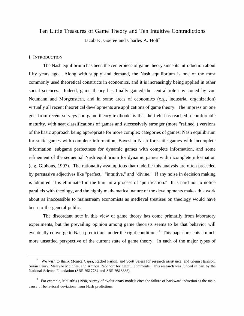
Figure 1 shows the frequencies for each 10-cent category centered around the claim label

on the horizontal axis. The lighter bars pertain to the high-R "treasure" treatment, where close

to 80 percent of all the subjects chose the Nash equilibrium strategy, with an average decision

of 201. However, roughly the same fraction chose thehighestpossible number in the low-R

treatment, for which the average was 280, as shown by the darker bars. Notice that the data in

the contradiction treatment are clustered at the opposite end of the set of feasible decisions from

the unique (rationalizable) Nash equilibrium.7

One might wonder whether the "anomalous" result for the low-R treatment disappears

6 The associated story is that two travelers purchase identical antiques while on a tropical vacation. Their luggageis lost on the return trip, and the airline asks them to make independent claims for compensation. In anticipation ofexcessive claims, the airline representative announces: "We know that the bags have identical contents, and we willentertain any claim between $180 and $300, but you will each be reimbursed at an amount that equals theminimumofthe two claims submitted. If the two claims differ, we will also pay a rewardR to the person making the smaller claimand we will deduct a penaltyR from the reimbursement to the person making the larger claim."

7 This result is statistically significant at all conventional levels, given the strong treatment and the relatively largenumber of independent observations (two paired observations for each of the 50 subjects). We will not report specificnon-parametric tests for cases that are so clearly significant. The individual choice data are provided in the DataAppendix for this paper on: http://www.people.virginia.edu/~cah2k/datapage.html.

7

when subjects play the game repeatedly and have the opportunity to learn. In Capra,et al.

Figure 1. Claim Frequencies in a Traveler’s Dilemmafor R = 180 (light bars) andR = 5 (dark bars)

(1999) we discuss the results of a repeated version of this game (with random matching) and

show that the opposite is true. Subjects chose numbers in the range [80, 200] withR = 5. The

average claimrosefrom approximately 180 in the first period to 196 in period 5, and the average

remained above 190 in later periods. Different cohorts played this game with different values

of R, and successive increasesR resulted in successive reductions in the average claims.8 None

of these treatment changes alter the unique Nash prediction of 80, so standard game theory

simply cannot explain the most salient feature of the data, i.e. the effect of the penalty/reward

parameter on average claims, a feature that is consistent with simple economic intuition.

8 With a penalty/reward parameter of 5, 10, 20, 25, 50, and 80 the average claims in the final three periods were195, 186, 119, 138, 85, and 81 respectively. Even though there is one treatment reversal, the effect of the penalty/rewardparameter on average claims is significant at the 1 percent level. Capra,et al. (1999) show that the patterns of adjustmentare well explained by a naive Bayesian learning model with decision error, and that the claim distributions for the finalfive periods are close to the distributions predicted by a logit equilibrium in the sense of McKelvey and Palfrey (1995,1996).

8

A Matching Pennies Game

Consider a symmetric matching pennies game in which the row player chooses between

TopandBottomand the column player simultaneously chooses betweenLeftandRight, as shown

in top part of Table 1. The payoff for the row player is $0.80 when the outcome is (Top, Left)

or (Bottom, Right) and $0.40 otherwise. The motivations for the two players are exactly

opposite: column earns $0.80 when row earns $0.40, and vice versa. Since the players have

opposite interests there is no equilibrium in pure strategies. Moreover, in order not to be

exploited by the opponent, neither player should favor one of their strategies, and the mixed-

strategy Nash equilibrium involves randomizing over both alternatives with equal probabilities.

As before, we obtained decisions from 50 subjects in a one-shot version of this game (5 cohorts

of 10 subjects, who were randomly matched and assigned row or column roles). The choice

percentages are shown in parentheses next to the decision labels in the top part of Table 1. Note

that the choice percentages are essentially "fifty-fifty," or as close as possible given that there

was an odd number of players in each role.

Now consider what happens if the row player’s payoff of $0.80 in the (Top, Left) box is

increased to $3.20, as shown in the asymmetric matching pennies game in the middle part of

Table 1. In a mixed-strategy equilibrium, a player’sown decision probabilities should be such

that theotherplayer is made indifferent between the two alternatives. Since the column player’s

payoffs are unchanged, the mixed-strategy Nash equilibrium predicts thatrow’s decision

probabilities do not change either. In other words, the row player should ignore the unusually

high payoff of $3.20 and still chooseTop or Bottom with probabilities of one-half. (Since

column’s payoffs are either 40 or 80 for playingLeft and either 80 or 40 for playingRight, row’s

decision probabilities must equal 1/2 to keep column indifferent betweenLeft and Right, and

hence willing to randomize.)9 This counter-intuitive prediction is dramatically rejected by the

data, with 96% of the row players choosing the Top decision that gives a chance of the high

$3.20 payoff. Interestingly, the column players seemed to have anticipated this, and they played

9 The predicted equilibrium probabilities for the row player are not affected if we relax the assumption of riskneutrality. Since there are only two possible payoff levels for column so without loss of generality columns’ utilities forpayoffs of 40 and 80 can be normalized to 0 and 1. Hence even a risk-averse column player will only be indifferent whenrow uses choice probabilities of 1/2.

9

Right 84% of the time, which is quite close their equilibrium mixed-strategy of 7/8. Next, we

Table 1. Three One-Shot Matching Pennies Games(with choice percentages)

SymmetricMatchingPennies

Left (48%) Right (52%)

Top (48%)(48%) 80, 40 40, 80

Bottom(52%)(52%) 40, 80 80, 40

AsymmetricMatchingPennies

Left (16%) Right (84%)

Top (96%)(96%) 320, 40 40, 80

Bottom(4%)(4%) 40, 80 80, 40

ReversedAsymmetry

Left (80%) Right (20%)

Top (8%)(8%) 44, 40 40, 80

Bottom(92%)(92%) 40, 80 80, 40

lowered the row player’s (Top, Left) payoff to $0.44, which again should leave the row player’s

own choice probabilities unaffected in a mixed-strategy Nash equilibrium. Again the effect is

dramatic, with 92% of the choices beingDown, as shown in the bottom part of Table 1. As

before, the column players seemed to have anticipated this reaction, playingLeft80% of the time.

To summarize, the unique Nash prediction is for the bolded row-choice percentages to be

unchanged at 50% for all three treatments. This prediction is violated in an intuitive manner,

with row players’ choices responding to their own payoffs. In this context,the Nash mixed-

10

strategy prediction seems to work only by coincidence, when the payoffs are symmetric.10

A Coordination Game with a Secure Outside Option

Games with multiple Nash equilibria pose interesting new problems for predicting

behavior, especially when some equilibria produce higher payoffs for all players. The problem

of coordinating on the high-payoff equilibrium may be complicated by the possible gains and

losses associated with payoffs that are not part of any equilibrium outcome. Consider a

coordination game in which players receive $1.80 if they coordinate on the high-payoff

equilibrium (H,H), $0.90 if they coordinate on the low-payoff equilibrium (L,L), and they receive

nothing if they fail to coordinate (i.e. when one player choosesH and the otherL). In addition,

the column player has a secure optionS that yields $0.40 for column and results in a zero payoff

for the row player. This game is given in Table 2 whenx = 0. To analyze the Nash equilibria

of this game, notice that for the column player a fifty-fifty combination ofL andH dominates

S, and a rational player should therefore avoid the secure option. EliminatingS turns the game

into a standard two-by-two coordination game that has three Nash equilibria: both players

choosingL, both choosingH, and a mixed-strategy equilibrium in which both players chooseL

with probability 2/3.

10 This anomaly is persistent when subjects play the game repeatedly. Ochs (1995) investigates a matching penniesgame with an asymmetry similar to that of the middle game in Table 1, and the row player’s continue to selectTopconsiderably more than one-half of the time, even after as many as fifty rounds. These results are replicated in McKelvey,Palfrey, and Weber (1997). We have also conducted some repeated matching pennies games that exactly match thosein Table 1, using 10 repetitions with the same partner. The results are qualitatively similar but less dramatic than thosein Table 1. One possible explanation for the weaker own-payoff effect in the repeated game is that there may be strategic"teaching" whereby a player may choose a particular strategy several times in a row in order to alter the other’s beliefsand decisions.

11

The Nash equilibria are independent ofx, which is the payoff to the row player when

Table 2. An Extended Coordination Game

L H S

L 90, 90 0, 0 x, 40

H 0, 0 180, 180 0, 40

(L,S) is the outcome, since the argument for eliminatingS is based solely on column’s payoffs.

However, the magnitude ofx may affect the coordination process: forx = 0, row is indifferent

betweenL andH when column selectsS, and row is likely to preferH when column does not

selectS (since thenL and H have the same number of zero payoffs for row, but the potential

positive payoff is higher with a choice ofH). Row is thus more likely to chooseH, which is

then also the optimal action for the column player. However, whenx is large, say 400, the

column player may anticipate that row will selectL in which case column should avoidH.

This intuition is borne out by the experimental data: in the treasure treatment withx = 0,

96 percent of the row players and 84 percent of the column players chose the high-payoff action

H, while in the contradiction treatment withx = 400 only 64 percent of the row players and 76

percent of the column players choseH. The percentages of outcomes that were coordinated on

the high-payoff equilibrium were 80 for the treasure treatment versus 32 for the contradiction

treatment. In the latter treatment, an additional 16 percent of the outcomes were coordinated on

the low-payoff equilibrium, but more than half of all the outcomes were uncoordinated, non-Nash

outcomes.

A Minimum-Effort Coordination Game

The next game we consider is also a coordination game with multiple equilibria, but in

this case the focus is on the effect of payoff asymmetries that determine the risks of deviating

in the upward and downward directions. The two players in this game choose "effort" levels

simultaneously, and the cost of effort determines the risk of deviation. The joint product is of

the fixed-coefficients variety, so that each person’s payoff is the minimum of the two efforts,

12

minus the product of the player’s own effort and a constant cost factor,c. In the experiment, we

let efforts be any integer in the range from 110 to 170. Ifc < 1, any common effort in this range

is a Nash equilibrium, because a unilateral one-unit increase in effort above a common starting

point will not change the minimum but will reduce one’s payoff byc. Similarly, a one-unit

decrease in effort will reduce one’s payoff by 1 -c, i.e. the reduction in the minimum is less than

the savings in effort costs whenc < 1. Obviously, a higher effort cost increases the risk of

raising effort and reduces the risk of lowering effort. Thus simple economic intuition suggests

that effort levels will be inversely related to effort costs, despite the fact that any common effort

level is a Nash equilibrium.

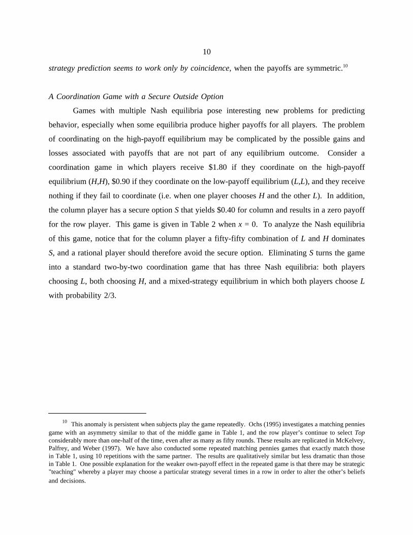
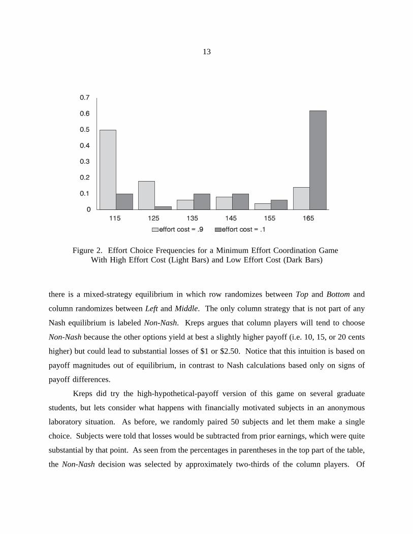
We ran one treatment with a low effort cost of 0.1, and the data for 50 randomly matched

subjects in this treatment are shown by the dark bars in Figure 2. Notice that behavior is quite

concentrated at the highest effort level of 170; subjects coordinate on the Pareto-dominant

outcome. The high effort cost treatment (c = 0.9), however, produced a preponderance of efforts

at the lowest possible level, as can be seen by the lighter bars in the figure. Clearly, the extent

of this "coordination failure" is affected by the key economic variable in this model in a manner

that is quite intuitive, even though Nash theory is silent.11

The Kreps Game

The previous examples demonstrate how the cold logic of game theory can be at odds

with intuitive notions about human behavior. This tension has not gone unnoticed by some game

theorists. For instance, Kreps (1995) discusses a variant of the game in the top part of Table 3

(where we have scaled back the payoffs to levels that are appropriate for the laboratory). The

pure-strategy equilibrium outcomes of this game are (Top, Left) and (Bottom, Right). In addition,

11 The standard analysis of equilibrium selection in coordination is based on the Harsanyi-Selten notion of riskdominance, which allows a formal analysis of the tradeoff between risk and payoff dominance. There is no agreementon how to generalize risk dominance beyond 2 × 2 games, but see Anderson, Goeree, and Holt (1998c) for a proposedgeneralization based on the "stochastic potential." Experiments with repeated plays of coordination games have shownthat behavior may begin near the Pareto-dominant equilibrium, but later converge to the equilibrium that is worst for allconcerned (van Huyck, Battalio, and Beil, 1990). Moreover, the equilibrium that is selected may be affected by the payoffstructure for dominated strategies (Cooperet al., 1992). See Goeree and Holt (1998) for results of a repeated coordinationgame with random matching. They show that the dynamic patterns of effort decisions are well explained by a simpleevolutionary model of noisy adjustment toward higher payoffs.

13

there is a mixed-strategy equilibrium in which row randomizes betweenTop and Bottomand

Figure 2. Effort Choice Frequencies for a Minimum Effort Coordination GameWith High Effort Cost (Light Bars) and Low Effort Cost (Dark Bars)

column randomizes betweenLeft andMiddle. The only column strategy that is not part of any

Nash equilibrium is labeledNon-Nash. Kreps argues that column players will tend to choose

Non-Nashbecause the other options yield at best a slightly higher payoff (i.e. 10, 15, or 20 cents

higher) but could lead to substantial losses of $1 or $2.50. Notice that this intuition is based on

payoff magnitudes out of equilibrium, in contrast to Nash calculations based only on signs of

payoff differences.

Kreps did try the high-hypothetical-payoff version of this game on several graduate

students, but lets consider what happens with financially motivated subjects in an anonymous

laboratory situation. As before, we randomly paired 50 subjects and let them make a single

choice. Subjects were told that losses would be subtracted from prior earnings, which were quite

substantial by that point. As seen from the percentages in parentheses in the top part of the table,

the Non-Nashdecision was selected by approximately two-thirds of the column players. Of

14

course, it is possible that this result is simply a consequence of "loss-aversion," i.e. the disutility

Table 3. Two Versions of the Kreps Game(with choice percentages)

BasicGame

Left (26%) Middle (8%) Non-Nash(68%) Right (0%)

Top (68%) 200, 50 0, 45 10, 30 20, -250

Bottom(32%) 0, -250 10, -100 30, 30 50, 40

PositivePayoffFrame

Left (24%) Middle (12%) Non-Nash(64%) Right (0%)

Top (84%) 500, 350 300, 345 310, 330 320, 50

Bottom(16%) 300, 50 310, 200 330, 330 350, 340

of losing some amount of money is greater than the utility associated with winning the same

amount (Kahneman, Knetsch, and Thaler, 1991). Since all the other columns contain negative

payoffs, loss-averse subjects would thus be naturally inclined to chooseNon-Nash. Therefore,

we ran another 50 subjects through the same game, but with 300 cents added to payoffs to avoid

losses, as shown in the bottom part of Table 3. The choice percentages shown in parentheses

indicate very little change, with close to two-thirds of column players choosingNon-Nashas

before. Finally, we ran 50 new subjects through the original version in the top part of the table,

with the (Bottom, Right) payoffs of (50, 40) being replaced by (350, 400), which (again) does

not alter the equilibrium structure of the game. With this admittedly heavy-handed enhancement

of the equilibrium in that cell, we observed 96%Bottomchoices and 84%Right choices, with

16% Non-Nashpersisting in this, the "treasure" treatment.

III. D YNAMIC GAMES WITH COMPLETE INFORMATION

As game theory became more widely used in fields like industrial organization, the

complexity of the applications increased to accommodate dynamics and asymmetric information.

15

One of the major developments coming out of these applications was the use of backward

induction rationality to eliminate equilibria with threats that are not "credible" (Selten, 1975).

Backward induction was also used to develop solutions to alternating-offer bargaining games

(Rubinstein, 1982), which was the first major advance on this historically perplexing topic since

Nash’s axiomatic approach. However, there have been persistent doubts that people will be able

to figure out complicated, multi-stage backward induction arguments. Rosenthal (1981) quickly

proposed a game, later dubbed the "centipede game," in which backward induction over a large

number of stages (e.g. 100 stages) was thought to be particularly problematic (e.g. McKelvey and

Palfrey, 1992). Many of the games in this section are inspired by Rosenthal’s (1981) doubts and

Beard and Beil’s (1994) experimental results. Indeed, the anomalies in this section are better

known than those in other sections, but we focus on very simple games with two or three stages,

using parallel procedures and subjects who have previously made a number of strategic decisions

in different one-shot games.

Should You Trust the Others to be Rational?

The power of backward induction is illustrated in the top game in Figure 3. The first

player begins by choosing between a safe decision,S, and a risky decision,R. If R is chosen,

the second player must choose between a decisionP that punishes both of them and a decision

N that leads to a Nash equilibrium that is also a joint-payoff maximum. There is, however, a

second Nash equilibrium where the first player choosesSand the second choosesP. The second

player has no incentive to deviate from this equilibrium because the self-inflicted punishment

occurs off of the equilibrium path. Subgame perfectness rules out this equilibrium by requiring

equilibrium behavior in each subgame, i.e. that the second player behave optimally in the event

that the second stage subgame is reached.

Again, we used 50 randomly paired subjects who played this game only once. The data

for this treasure treatment are quite consistent with the subgame perfect equilibrium; the

preponderance of first players trust the other’s rationality enough to chooseR, and there are no

irrational P decisions that follow. The game shown in the bottom part of Figure 3 is identical,

except that the second player only forgoes 2 cents by choosingP. This change does not alter the

16

fact that there are two Nash equilibria, one of which is ruled out by subgame perfectness. The

Figure 3. Should You Trust the Rationality of Others?

choice percentages for 50 subjects indicate that a majority of the first players did not trust others

to be perfectly rational when the cost of irrationality is so small. Only about a third of the

outcomes matched the subgame perfect equilibrium in this game.12 We did a third treatment

(not shown) in which we multiplied all payoffs by a factor of 5, except that theP decision led

to (100, 348) instead of (100, 340). This large increase in payoffs produced an even more

dramatic result; only 16% of the outcomes were subgame perfect, and 80% of the outcomes were

at the Nash equilibrium that is not subgame perfect.

Are "Credible" Threats Really Credible?

The game just considered is a little unusual in that the second player has no reason to

12 See Beard and Beil (1994) for similar results in a two-stage game played only once.

17

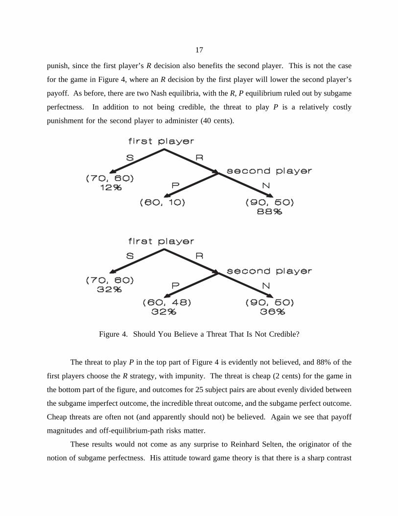
punish, since the first player’sR decision also benefits the second player. This is not the case

for the game in Figure 4, where anR decision by the first player will lower the second player’s

payoff. As before, there are two Nash equilibria, with theR, P equilibrium ruled out by subgame

perfectness. In addition to not being credible, the threat to playP is a relatively costly

punishment for the second player to administer (40 cents).

The threat to playP in the top part of Figure 4 is evidently not believed, and 88% of the

Figure 4. Should You Believe a Threat That Is Not Credible?

first players choose theR strategy, with impunity. The threat is cheap (2 cents) for the game in

the bottom part of the figure, and outcomes for 25 subject pairs are about evenly divided between

the subgame imperfect outcome, the incredible threat outcome, and the subgame perfect outcome.

Cheap threats are often not (and apparently should not) be believed. Again we see that payoff

magnitudes and off-equilibrium-path risks matter.

These results would not come as any surprise to Reinhard Selten, the originator of the

notion of subgame perfectness. His attitude toward game theory is that there is a sharp contrast

18

between standard theory and behavior. For a long time he essentially wore different hats when

he did theory and ran experiments, although his 1995 Nobel prize was clearly for his

contributions in theory. This schizophrenic stance may seem inconsistent, but it may prevent

unnecessary anxiety, and some of Selten’s recent theoretical work is based on models of

boundedly rational (directional) learning (Selten and Buchta, 1994). In contrast, John Nash was

reportedly discouraged by the predictive failures of game theory and gave up on both

experimentation and game theory (Nasar, 1998, p.150).

Two-Stage Bargaining Games

Bargaining has long been considered a central part of economic analysis, and at the same

time, one of the most difficult problems for economic theory. One promising approach is to

model unstructured bargaining situations "as if" the parties take turns making offers, with the

costs of delayed agreement reflected in a shrinking size of the pie to be divided. This problem

is particularly easy to analyze when the number of alternating offers is fixed and small.

Consider a bargaining game in which each player gets to make a single proposal for how

to split a pie, but the amount of money to be divided falls from $5 in the first stage to $2 in the

second. The first player proposes a split of $5 that is either accepted (and implemented) or

rejected, in which case the second player proposes a split of $2 that is either accepted or rejected

by the first player. This final rejection results in payoffs of zero for both players, so the second

player can (in theory) successfully demand $1.99 in the second stage if the first player prefers

a penny to nothing. Knowing this, the first player should demand $3 and offer $2 to the other

in the first stage. In a subgame perfect equilibrium, the first player receives the amount by which

the pie shrinks, so a larger cost of delay confers a greater advantage to the player making the

initial demand, which seems reasonable. For example, a similar argument shows that if the pie

shrinks by $4.50, from $5 to $0.50, then the first player should make an initial demand of $4.50.

We used 60 subjects (6 cohorts of 10 subjects each), who were randomly paired for each

of the two treatments described above (alternating in order and separated by other one-shot

games). The average demand for the first player was $2.83 for the $5/$2 treatment, with a

standard deviation of $0.29. This is quite close to the predicted $3.00 demand, and 14 of the 30

initial demands were exactly equal to $3.00 in this treasure treatment. But the average demand

19

only increased to $3.38 for the other treatment with a $4.50 prediction, and 28 of the 30 demands

were below the prediction of $4.50. Rejections were quite common in this treatment with higher

demands and correspondingly lower offers to the second player, which is not surprising given the

smaller costs of rejecting "stingy" offers.

These results fit into a larger pattern surveyed in Davis and Holt (1993, chapter 5) and

Roth (1995); initial demands in two-stage bargaining games tend to be "too low" relative to

theoretical predictions when the equilibrium demand is high, say more than 80% of the pie as

in our $5.00/$0.50 treatment, and initial demands tend to be close to predictions when the

equilibrium demand is 50-75% of the pie (as in our $5.00/$2.00 treatment). Interestingly, initial

demands are "too high" when the equilibrium demand is less than half of the pie. Here is an

example of why theoretical explanations of behavior should not be based on experiments in only

one part of the parameter space, and why theorists should have more than just a casual, second-

hand knowledge of the experimental economics literature.13 Many of the diverse theoretical

explanations for anomalous behavior in bargaining games hinge on models of preferences in

which a person’s utility depends on the payoffs of both players, i.e. distribution matters (Bolton,

1998, Bolton and Ockenfels, 1999, and Fehr and Schmidt, 1997). The role of fairness is

illustrated dramatically in the experiment reported in Goeree and Holt (2000a), who obtained

even larger deviations from subgame perfect Nash predictions than those reported here by giving

subjects asymmetric money endowments that raise fairness issues without altering the subgame

perfect Nash prediction.

IV. STATIC GAMES WITH INCOMPLETE INFORMATION

Vickrey’s models of auctions with incomplete information constitute one of the most

widely used applications of game theory. If private values are drawn from a uniform distribution,

the Bayesian Nash equilibrium predicts that bids will be proportional to value, which is generally

consistent with laboratory evidence. The main deviation from theoretical predictions is the

tendency of human subjects to "overbid," which is commonly rationalized in terms of risk

13 Another example is the development of theories of generalized expected utility to explain "fanning out"preferences in Allais paradox situations, when later experiments in other parts of the probability triangle found "fanningin."

20

aversion, an explanation that has lead to some controversy. Harrison (1989), for instance, argues

that deviations from the Nash equilibrium may well be caused by a lack of monetary incentives

since the costs of such deviations are rather small: the "flat maximum critique." Our approach

here is to specify two auction games with identical Nash equilibria, but with differing incentives

not to overbid.

First, consider a game in which each of two bidders receives a private value for a prize

to be auctioned in a first-price, sealed bid auction. In other words, the prize goes to the highest

bidder for a price equals that bidder’s own bid. Each bidder’s value for the prize is equally

likely to be $0, $2, or $5. Bids are constrained to be integer dollar amounts, with ties decided

by the flip of a coin.

The relevant Nash equilibrium in this game with incomplete information about others’

Table 4. Equilibrium Expected Payoffs for the (0,2,5) Treatment(Optimal Bids Are Denoted by an Asterisk *)

bid = 0 bid = 1 bid = 2 bid = 3 bid = 4 bid = 5

value = $0 0* -.5 -1.66 - 3 - 4 - 5

value = $2 .33 .5* 0 -1 -2 - 3

value = $5 .83 2 2.5* 2 1 0

preferences is the Bayesian Nash equilibrium, which specifies an equilibrium bid for each

possible realization of a bidder’s value. It is straightforward but tedious to verify that the Nash

equilibrium bids are $0, $1, and $2 for a value of $0, $2, and $5 respectively, as can be seen

from the equilibrium expected payoffs in Table 4. For example, consider a bidder with a private

value of $5 (in the bottom row) who faces a rival that bids according to the proposed Nash

solution. A bid of 0 has a 1/2 chance of winning (decided by a coin flip) if the rival’s value, and

hence the rival’s bid, is zero, which happens with probability 1/3. Therefore, the expected payoff

of a zero bid with a value of $5 equals 1/2*1/3*($5 - $0) = $5/6 = .83. If the bid is raised to

$1, the probability of winning becomes 1/2 (1/3 when the rival’s value is $0 plus 1/6 when the

rival’s value is $2). Hence, the expected payoff of a $1 bid is 1/2*($5 - $1) = $2. The other

numbers in Table 4 are derived in a similar way. The maximum expected payoff in each row

21

coincides with the equilibrium bid, as indicated by an asterisk (*). Note that the equilibrium

involves bidding about one half of the value.14

Table 5 shows the analogous calculations for the second treatment, with equally likely

Table 5. Equilibrium Expected Payoffs for the (0,3,6) Treatment(Optimal Bids Are Denoted by an Asterisk *)

bid = 0 bid = 1 bid = 2 bid = 3 bid = 4 bid = 5

value = $0 0* -.5 -1.66 - 3 - 4 - 5

value = $3 .5 1* .83 0 -1 - 2

value = $6 1 2.5 3.33* 3 2 1

private values of $0, $3, or $6. Interestingly, this increase in values does not alter the

equilibrium bids in the unique Bayesian Nash equilibrium, as indicated by the location of optimal

bids for each value. Even though the equilibria are the same, we expected more of an upward

bias in bids in the second (0, 3, 6) treatment. The intuition can be seen by looking at payoff

losses associated with deviations from the Nash equilibrium. Consider, for instance, the middle-

value bidder with expected payoffs shown in the second rows of Tables 4 and 5. In the (0, 3,

6) treatment, the cost of bidding $1 above the equilibrium bid is $1 - $0.83 = $0.17, which is less

than the cost of bidding $1 below the equilibrium bid: $1 - $0.50 = $0.50. In the (0, 2, 5)

treatment, the cost of an upward deviation from the equilibrium bid is greater than the cost of

a downward deviation, see the middle row of Table 4. A similar argument applies to the high-

value bidders, while deviation costs are the same in both treatments for the low-value bidder.

Hence we expected more overbidding for the (0, 3, 6) treatment.

This intuition is borne out by bid data for the 50 subjects who participated in a single

auction under each condition. Eighty percent of the bids in the (0, 2, 5) treatment matched the

equilibrium: the average bids for low, medium, and high value bidders were $0, $1.06, and $2.64

14 The bids would be exactly half of value if the highest value were $4 instead of $5, but we had to raise thehighest value to eliminate multiple Nash equilibria.

22

respectively. In contrast, the average bids for the (0, 3, 6) treatment were $0, $1.82, and $3.40

Table 6. Bid Frequencies (Equilibrium Bids Marked with an Asterisk *)

(0, 2, 5) treatment (0, 3, 6) treatment

bid frequency bid frequency

value = 0 0* 20 value = 0 0* 17

value = 2 1* 15 value = 3 1* 5

2 1 2 11

3 0 3 2

value = 5 1 1 value = 6 1 0

2* 5 2* 3

3 6 3 4

4 2 4 6

5 0 5 1

6 0 6 1

for the three value levels. The bid frequencies for each value are shown in Table 6. As in

previous games, deviations from Nash behavior in these private value auctions seem to be

sensitive to the costs of deviation. Of course, this does not rule out the possibility that risk

aversion or some other factor may also have some role in explaining the overbidding observed

here, especially the slight overbidding for the high value in the (0, 2, 5) treatment.15

V. DYNAMIC GAMES WITH INCOMPLETE INFORMATION: SIGNALING

Signaling games are complex and interesting because the two-stage structure allows an

15 Goeree, Holt, and Palfrey (1999) report a first-price auction experiment with 6 possible values, under repeatedrandom matching for ten periods. An econometric model that includes both decision error and risk aversion provides agood fit of the data. Several plausible alternatives to risk aversion, like nonlinear cumulative probability weighting ora "joy of winning," are considered. Lucking-Reiley (1999) mentions risk aversion as a possible explanation foroverbidding in a variety of auction experiments.

23

opportunity for players to make inferences and change others’ inferences about private

information. This complexity often generates multiple equilibria that, in turn, have stimulated

a sequence of increasingly complex refinements of the Nash equilibrium condition. Although it

is unlikely that introspective thinking about the game will produce equilibrium behavior in a

single play of a game this complex (except by coincidence), the one-shot play reveals useful

information about subjects’ cognitive processes.

In the experiment, half of the subjects were designated as "senders" and half as

Table 7. Signaling with a Separating Equilibrium(sender’s payoff, responder’s payoff)

response to Left signal response to Right signal

C D E C D E

type AsendsLeft

300, 300 0, 0 500, 300type AsendsRight

450, 900 150, 150 1000, 300

type BsendsLeft

500, 500 300, 450 300, 0type BsendsRight

450, 0 0, 300 0, 150

"responders." After reading the instructions, we began by throwing a die for each sender to

determine whether the sender was of type A or B. Everybody knew that theex anteprobability

of a type A sender was 1/2. The sender, knowing his/her own type would choose a signal,Left

or Right. This signal determined whether the payoffs on the right or left side of Table would be

used. (The instructions used letters to identify the signals, but we will use words here to

facilitate the explanations.) This signal would be communicated to the responder that was

matched with that sender. The responder would see the sender’s signal,Left or Right, but not

the sender’s type, and then choose a response,C, D, or E. The payoffs were determined by

Table 7, with the sender’s payoff to the left in each cell.

First, consider the problem facing a type A sender, for whom the possible payoffs from

sending aLeft signal (300, 0, 500) seem, in some loose sense, is less attractive than those for

24

sending aRightsignal (450, 150, 1000). (For example, if each response is thought to be equally

likely, then theRightsignal has a higher expected payoff.) Consequently, theRightrow has been

shaded in the top right part of the table. Similarly, a type B sender looking at the payoffs in the

bottom row of the table might be more attracted by theLeft signal, with payoffs of (500, 300,

300) as compared with (450, 0, 0).16 Therefore, the payoffs for type B sending theLeft signal

have been shaded. In fact, all of the type B subjects did send theLeft signal, and 7 of the 10

type A subjects sent theRightsignal. All responses in this game wereC, so all but three of the

outcomes were in the two boxes that have thick outlines. Notice that this is an equilibrium, since

neither type of sender would benefit from sending the other signal, and the respondent cannot do

any better than the maximum payoff received in the boxes. This is a separating Nash

equilibrium; the signal reveals the sender’s type.

The payoff structure for this game becomes a little clearer if you think of the responses

as one of three answers to a request: Concede, Deny, or Evade. Evade is sufficiently unattractive

to respondents that it is never selected, so consider the other two responses and note that a sender

always prefers that the responder choose Concede instead of Deny. In the separating equilibrium,

the signals reveal the senders’ types, the responder always Concedes, and all players are satisfied.

There is, however, a second equilibrium for the game in Table 7 in which the responder

Concedes toLeft and DeniesRight, and therefore both sender types sendLeft to avoid being

Denyed. To check that the responder has no incentive to deviate, note that Concede is a best

response to aLeft regardless of the sender’s type, and that Deny is a best response to a deviant

Right signal if the responder believes that it was sent by a type B. Backward induction

rationality (of the sequential Nash equilibrium) does not rule out these beliefs, since a deviation

does not occur in equilibrium, and the respondent is making a best response to the beliefs. What

is unintuitive about these beliefs (that a deviantRight signal comes from a type B) is that the

type B is earning 500 in this (Left, Concede) equilibrium outcome, and no deviation could

conceivably increase this payoff, whereas, the type A is earning 300 in theLeft side pooling

equilibrium, and this type could possibly earn more (450 or even 1000), depending on the

16 These are not dominance arguments, since the responder can respond differently to each signal, and the lowestpayoff from sending one signal is not higher than the highest payoff that can be obtained from sending the other signal.

25

response to a deviation. The Cho and Kreps (1987)intuitive criterionrules out these beliefs, and

therefore, selects the separating equilibrium that was observed in the treasure treatment.

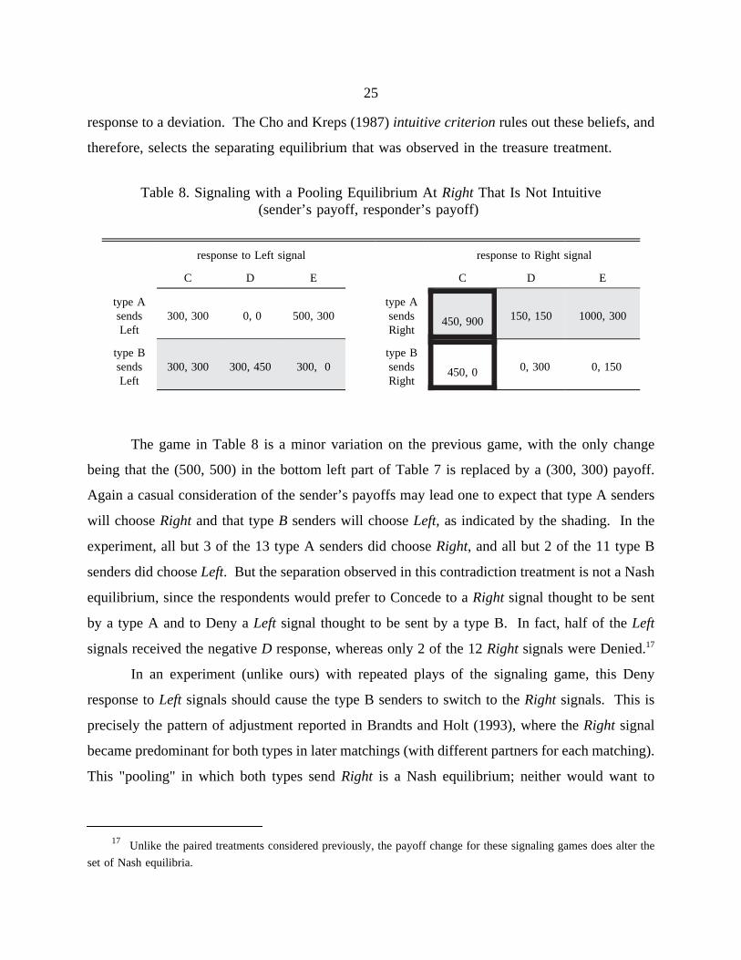
The game in Table 8 is a minor variation on the previous game, with the only change

Table 8. Signaling with a Pooling Equilibrium AtRight That Is Not Intuitive(sender’s payoff, responder’s payoff)

response to Left signal response to Right signal

C D E C D E

type AsendsLeft

300, 300 0, 0 500, 300type AsendsRight

450, 900 150, 150 1000, 300

type BsendsLeft

300, 300 300, 450 300, 0type BsendsRight

450, 0 0, 300 0, 150

being that the (500, 500) in the bottom left part of Table 7 is replaced by a (300, 300) payoff.

Again a casual consideration of the sender’s payoffs may lead one to expect that type A senders

will chooseRight and that typeB senders will chooseLeft, as indicated by the shading. In the

experiment, all but 3 of the 13 type A senders did chooseRight, and all but 2 of the 11 type B

senders did chooseLeft. But the separation observed in this contradiction treatment is not a Nash

equilibrium, since the respondents would prefer to Concede to aRight signal thought to be sent

by a type A and to Deny aLeft signal thought to be sent by a type B. In fact, half of theLeft

signals received the negativeD response, whereas only 2 of the 12Rightsignals were Denied.17

In an experiment (unlike ours) with repeated plays of the signaling game, this Deny

response toLeft signals should cause the type B senders to switch to theRight signals. This is

precisely the pattern of adjustment reported in Brandts and Holt (1993), where theRight signal

became predominant for both types in later matchings (with different partners for each matching).

This "pooling" in which both types sendRight is a Nash equilibrium; neither would want to

17 Unlike the paired treatments considered previously, the payoff change for these signaling games does alter the

set of Nash equilibria.

26

switch if they anticipated receiving aD response to theLeft signal. Of course, theD response

to Left is only appropriate if the respondent thinks the deviantLeft signal comes from a type B

sender. But these beliefs about the deviant are ruled out by the intuitive criterion argument given

above: the type B sender gets 450 in the poolingRight equilibrium, and there is no payoff on

the left side of the bottom row of table 8 that would be better for this sender type. In contrast,

the type A sender who also gets 450 in equilibrium, could possibly get a 500 payoff (from an

E response) to a deviation on the top row, left side of the table. There is a second Nash

equilibrium for the game in Table 8: both types sendLeft and respondent Concedes toLeft and

DeniesRight. The beliefs that support these responses, that a deviant Right signal is sent by a

type B, are not ruled out by the intuitive criterion, since the type B sender could possibly obtain

a payoff increase (from 300 to 450) from such a deviation. There is no support for this

"intuitive" equilibrium, either in the one-shot games or in repeated-matching design of Brandts

and Holt.18

The important lesson from this contradiction treatment is that restrictions on what beliefs

are "reasonable" must be derived from an analysis of the process of adjustment to equilibrium.

Once people get to an equilibrium (e.g. with both types sending signalRight), when the

respondent sees a deviant signal, the inference about the type that deviated will be based on the

type that tended to send that signal in the past, before behavior converged to the other signal.

In repeated signaling games, beliefs "off the equilibrium path" are determined by the out-of-

equilibrium behavior actually observed earlier during the process of adjustment. This learning-

based analysis of beliefs can be quite different from the deductive analysis used in the

refinements literature, which begins by looking at what payoffs playersdo get in equilibrium and

then looking at which type of sender could conceivably do better by deviating. In addition, a

better understanding of behavior in one-shot games, however complex, will help us predict the

initial type/signal correlation that may have a big influence on respondents’ beliefs even after one

18 This is essentially the refinement recommended by Gibbons (1997) for this type of game, and any equilibriumruled out by the intuitive criterion in a two-stage signaling game will be ruled out by stronger refinements like "divinity"or "strategic stability." Cho and Kreps (1987) show that, in the context of these two-stage signaling games, anyequilibrium ruled out by the intuitive criterion will also be ruled out by stronger refinements like "divinity" or "strategicstability," so the Brandts and Holt (1993) experiment is inconsistent with these refinements as well.

27

of the signals is no longer being used very often in later periods of a repeated game.

VI. NOISY DECISION MAKING AND INTROSPECTION INONE-SHOT GAMES

A Nash equilibrium can be found by considering only thesignsof payoff differences.

The games considered thusfar indicate that payoffmagnitudesmay matter, and that the directions

of deviation from Nash may be affected by payoff asymmetries. Biases in behavior can be self-

reinforcing in a dramatic manner in situations with a lot of payoff interdependence, as in a

traveler’s dilemma. In all of the games considered, however, there are payoff conditions where

Nash or the relevant refinement yields accurate predictions. This section describes a model of

noisy introspection that is intended to explain both the treasures and the contradictions for these

one-shot games. Recall that the Nash equilibrium requires perfect payoff maximization (no

errors) and consistency of actions and beliefs (no surprises). Our approach is to allow decision

errors that are sensitive to the magnitudes of payoff differences, as in a logit probabilistic choice

model. Play in many types of one-shot games is likely to contain surprises, no matter how

carefully players think about the payoffs before deciding. Therefore, we also relax the second

Nash assumption, that of consistency of actions and beliefs, by introducing a process of iterated

stochastic conjectures.

A payoff-sensitive choice rule can be based on an assumption that decision probabilities

are positively related to expected payoffs. The logit rule, for example, specifies that the choice

probabilities, pi, for options i = 1,...,m, are proportional to an exponential function of the

associated expected payoffsπie:

where the sum in the denominator ensures that the probabilities sum to one. The expected

(1)

payoffs in (1) are determined by a player’s beliefs about the rival. Letqi, i = 1,...,m, denote

players’ "belief probabilities." For instance, if a player thinks that all options are equally likely

to be chosen by the opponent, thenqi is simply 1/m for all i. The logit choice rule (1) maps

belief probabilities to choice probabilities, i.e.p = φµ(q), whereφµ represents the map on the right

28

side of (1). The "error parameter," µ, determines how sensitive choice probabilities are to payoff

differences. As µ goes to infinity, the arguments of the exponential expressions go to zero, and

the probabilities go to 1/m, regardless of expected payoffs. Thus a high µ represents noisy

decision making that makes choices essentially random. In contrast, dividing expected payoffs

by a low value of µ means that payoff differences are blown up, making choice probabilities

sensitive to payoff differences. Hence the "noisy best response" rule in (1) includes perfectly

rational behavior and completely random behavior as limiting cases.

We model the process of pre-play introspection as being stochastic, since it is very likely

that speculation about others’ decisions is highly subjective. Consider a symmetric, two-player

game in normal form withm decisions for each player. The simplest way to proceed is to begin

introspection by assuming that all possible decisions made by the other player are equally likely,

and use the 1/m probabilities to calculate the expected payoffs,πie, associated with each decision.

These expected payoffs can be used in (1) to generate a new set of conjectured probabilities,

those that are logit probabilistic responses to the initial conjectures. Iterating in this manner, the

thought process will produce more refined conjectures.19 However, this iterative procedure

becomes increasingly complex, and we will assume that the error rate grows (geometrically) with

each further iteration. With a vector of initial belief probabilities,p0, the vector of noisy best

response probabilities is given by the logit functions in (1):p = φµ(p0), where µ is an error rate

associated with the decision. There is likely to be more error associated with beliefs about the

other player’s responses, so we increase the error parameter for one iteration tot µ, wheret > 1.

Thus p = φµ(φtµ(p0)) represents the noisy (µ) responses to an even noisier (tµ) response top0.

This process can be iterated backwards, with the "telescoping" parametert > 1 determining how

fast the error rate blows up with further iterations; the error rate for thenth iteration is given by

19 For an alternative approach, see Capra (1998). In her model, beliefs are represented by degenerate distributionsthat put all probability mass at a single point. The location of the belief points is,ex ante, stochastic. A deterministicmodel of introspection in 2 × 2 games is presented in Olcina and Urbano (1994). This model uses an axiomatic approachto select a prior distribution, which is revised by a simulated learning process. This latter process is essentially a partialadjustment from current beliefs to best responses to current beliefs. The model has the attractive property that it selectsthe risk-dominant Nash equilibrium. Since the simulated learning process has no noise, it will converge to the uniqueNash equilibrium in mixed strategies in the asymmetric matching pennies games, which is an undesirable feature of themodel in light of the one-shot data reported here. Our conjecture is that it will not track data patterns in the traveler’sdilemma game either, since the (noise-free) best-responses in this game are unaffected by the magnitude of theRparameter that has such a large impact on the observed decisions.

29

tn-1 µ. We are interested in the choice probabilities in the limit as the number of iterations goes

to infinity:

One issue is whether the limit in (2) converges. In Goeree and Holt (2000b) we use

(2)

continuity arguments to show that this limit is well defined fort > 1. A second issue is what to

do about the seemingly arbitrary initial probability vector. Note that, sinceφ∞ maps the whole

probability simplex to a single point, the process is independent of the initial belief vectorp0.

The geometrically increasing error rate in (2) captures the idea that it becomes more and more

complex to think further back. For at value between 2 and 4, say, the process converges quickly

and the iterated probabilities remain more or less the same after several steps.20 Finally, the

limit caset = 1 is of special interest. For some games (e.g. matching pennies) the process will

not converge whent = 1, but when it does, the limit probabilities,p*, must be invariant under

the logit map:φµ(p*) = p*. A fixed point of this type constitutes a "logit equilibrium," which

is a special case of the quantal response equilibrium defined in McKelvey and Palfrey (1995,

1996). It is in this sense that the logit equilibrium arises as a limit case of the noisy introspective

process defined in (2). Whent > 1, the choice probabilities on the left side of (2) generally do

not match the belief probabilities at any stage of the iterative process on the right. In other

words, the introspective process allows for surprises, which are likely to occur in oneshot games.

For given values of the telescope and error parameters, the predicted distribution of

decisions can be found by iterating the stochastic best responses to any initial distribution,

20 The convergence proof in Goeree and Holt (2000b) allows the telescope parameter to be person specific and todiffer for different levels of introspection. The only restriction is that the telescope parameters be strictly positive andthat there be more noise at higher levels of iteration. Instead of increases in error parameters from µ totµ to t2µ ..., forexample, the increase can be from µ tot1µ to t2µ, where 1 <t1 < t2. This formulation is flexible and allows many specialcases. Ift1 is very large, the model essentially generates a µ stochastic best response to a uniform distribution over allof the other player’s decisions, which is the way we start the simulations in Capra,et al. (1999). Similarly, if µ =∞, thechoice probabilities on the left side of (2) are uniform as is the case for Stahl and Wilson’s (1995) "level-0 rationality."If µ goes to zero andt goes to infinity, we have a (non-stochastic) best response to a uniform distribution, whichcorresponds to Stahl and Wilson’s "level 1 rationality." Higher levels can be generated similarly. Roughly speaking, lowvalues oft in our model correspond to higher rationality levels in their formulation, in the sense that the precision of thethought process is relatively insensitive to the number of iterations. Rather than assuming a fixed number of iterations,(2) allows parsimonious representation of a wide range of rationality levels.

30

starting with tn-1µ and reducingn until reaching 1 for the final (µ) stochastic response. The

outcome of this process is typically independent of the starting value ofn, as long as it is larger

than 5 or 6, but we use higher values just to be safe. With asymmetries, there is a noisy best

response function for each player, and these functions alternate in the iteration process in (2).

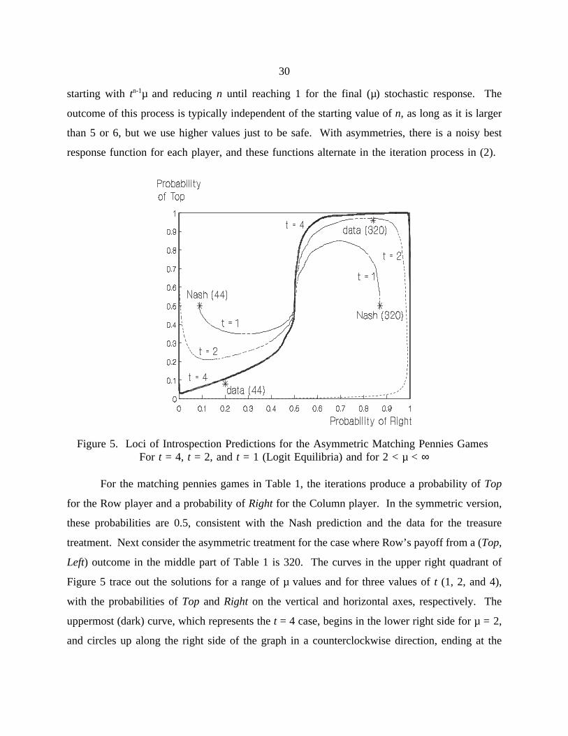
For the matching pennies games in Table 1, the iterations produce a probability ofTop

Figure 5. Loci of Introspection Predictions for the Asymmetric Matching Pennies GamesFor t = 4, t = 2, andt = 1 (Logit Equilibria) and for 2 < µ < ∞

for the Row player and a probability ofRight for the Column player. In the symmetric version,

these probabilities are 0.5, consistent with the Nash prediction and the data for the treasure

treatment. Next consider the asymmetric treatment for the case where Row’s payoff from a (Top,

Left) outcome in the middle part of Table 1 is 320. The curves in the upper right quadrant of

Figure 5 trace out the solutions for a range of µ values and for three values oft (1, 2, and 4),

with the probabilities ofTop and Right on the vertical and horizontal axes, respectively. The

uppermost (dark) curve, which represents thet = 4 case, begins in the lower right side for µ = 2,

and circles up along the right side of the graph in a counterclockwise direction, ending at the

31

center point (0.5, 0.5) as µ goes to infinity. Notice that this line passes near the asterisk at (0.84,

0.96) which represents the actual choice proportions for the "320" contradiction treatment. The

curve in the lower left part of the figure is the analogous locus for the "44" contradiction

treatment (bottom part of Table 1), and again this line passes close to the asterisk representing

the data proportions. The dashed curves in upper-right and lower-left regions represent the loci

of solutions witht values of 1 and 2. Thet = 1 case traces the logit equilibria, starting at the

Nash mixed equilibria for the case of no error, µ = 0, and again ending up in the center as µ goes

to infinity.21 Unlike the one-shot game case, many of the deviations from Nash predictions in

games with repeated random matching are well approximated by a logit equilibrium (McKelvey

and Palfrey, 1995; Goeree and Holt, 1999; Reynolds, 1999).

Space constraints prevent a detailed analysis of each of the ten treasure/contradiction

games presented here, but in the remainder of this section we will sketch how the introspective

model explains the qualitative features of conformity in the treasure treatments and divergence

from Nash predictions in the contradiction treatments. To derive point predictions we need to

fix values for the error and telescope parameters: we use out-of-sample estimates of µ = 6 (from

Capraet al., 2000) andt = 4 (from Goeree and Holt, 2000b). The introspection model tracks the

data in the traveler’s dilemma quite closely, producing predicted claim averages of 180 forR =

180 and 280 forR = 5, while the actual data averages were 201 and 280 respectively. The

predictions of the introspective model also conform nicely with the data in the coordination game

that has a range of Nash equilibria for each integer on [110, 170]: the prediction and data

averages are 155 and 156 respectively for the low-effort-cost treatment and 125 and 130 for the

high-effort-cost treatment. The introspection model predicts the general pattern of behavior for

the matrix coordination game in Table 2 and the prevalence of Non-Nash decisions by Column

in Table 3, but the effects of the treatment change are "over-predicted" in each case.22

21 It may not be a coincidence that thet = 4 lines fit reasonably well. We used maximum-likelihood techniqueson data from 32 (unrelated) one-shot 2 × 2 matrix games to estimatet = 4.1 (.4), with the standard error in parentheses.The data were for a series of variations of prisoner’s dilemma, chicken, and matching pennies games, both symmetric andasymmetric, as reported in Goeree and Holt (2000b).

22 For Table 2, the predicted rate of coordination on the (H, H) outcome whenx = 0 is 100%, whereas the subjectsonly achieved an 80% coordination rate. Withx = 400, the predicted coordination rate on the (L, L) outcome is 83%,as compared to only 16% in the data. A similar pattern is observed for the Kreps game in Table 3: the introspection

32

Table 9 shows data for the two-stage Trust Game in Figure 3 and the Threat Game in

Table 9. Two-Stage Trust and Threat Games: Data Averages (Introspection Predictions)

TreatmentSafe Outcome

(not subgame perfect)(S)

PunishmentOutcome

(R, P)

Risky Outcome(subgame perfect nash)

(R, N)

Trust Game(Figure 3)

Treasure 16% (36%) 0% (0%) 84% (64%)

Contradiction 52% (98%) 12% (1%) 36% (1%)

Threat Game(Figure 4)

Treasure 12% (8%) 0% (0%) 88% (92%)

Contradiction 32% (28%) 32% (30%) 36% (42%)

Figure 4. The introspection predictions are shown in parentheses to the right of the data

averages. These predictions generally track the data shifts away from the "risky" subgame-

perfect Nash decision when the cost of punishment is reduced to 2 cents, although this shift is

strongly over-predicted for the Trust Game treatments in the top two rows. The introspection

model also predicts the failure of the proposers to fully capitalize on their strategic advantage in

the two-stage bargaining games. For the treasure treatment with a Nash demand of 300, the data

and introspection predictions are 283 and 270 respectively, whereas with a Nash demand of 450

the data and introspection predictions are 338 and 371 respectively. For the signaling game, the

introspection model predicts the strong separation observed in the data, both when it is a Nash

equilibrium (treasure) and when it is not (contradiction). In the private value auction, the

introspection correctly predicts higher bids in the (0, 3, 6) treatment with low upside risk, as

observed in the data. But the slight overbidding for the treasure treatment is not predicted, which

may be due to risk aversion or some other omitted factor.

The analysis of introspection is a relatively understudied topic in game theory, as

compared with equilibrium refinements and learning, for example. Our model of noisy iterated

introspection does a fairly good job of organizing the qualitative patterns of conformity and

model (with µ = 6 andt = 4) predicts that 100% of the column decisions will be on the Non-Nash decision, as comparedto 68% in the data, and the heavy-handed treasure treatment that raises the (Bottom, Right) payoffs is predicted to drawabout 99% of Row and Column decisions, whereas the data averages are 96% and 84%.

33

deviation from the predictions of standard theory, but there are obvious discrepancies. We hope

that this paper will stimulate further theoretical work on models of behavior in one-shot games.

One potentially useful approach may be to elicit beliefs directly as the games are played (Schotter

and Narkov, 1998; Offerman, 1997).

VII. CONCLUSION

Games played only once are interesting because many games are in fact only played once;

single play is especially relevant in applications of game theory in other fields, e.g. international

conflicts, election campaigns, and legal disputes. The decision makers in these contexts, like the

subjects in our experiments, typically have experience in similar games with other people. One-

shot games are also appealing because they allow us to abstract away from issues of learning and

attempts to manipulate others’ beliefs, behavior, or preferences (e.g. cooperativeness). This paper

reports the results of ten pairs of games that are played only once by subjects who have

experience with other one-shot and repeated games. The Nash equilibrium (or relevant

refinement) provides accurate predictions for standard versions of these games. In each case,

however, there is a matched game for which the Nash prediction clearly fails, although it fails

in a way that is consistent with economic intuition. The results for these experienced subjects

show:

1) Behavior may diverge sharply from the unique rationalizable (Nash) equilibrium in a

social (traveler’s) dilemma. In these games, the Nash equilibrium is located on one side of the

range of feasible decisions, and data for the contradiction treatment have a mode on theopposite

side of this range. The most salient feature of the data is the extreme sensitivity to a parameter

that has no effect on the Nash outcome.

2) Students suffering through game theory classes may have good reasons when they have

trouble understanding why a change in one player’s payoffs only affects theother player’s

decision probabilities in a mixed-strategy Nash equilibrium. The data from matching pennies

experiments show strong "own-payoff" effects that are not predicted by the unique (mixed-

strategy) Nash equilibrium. The Nash analysis seems to work only by coincidence, when the

payoff structure is symmetric and deviation risks are balanced.

3) Effort choices are strongly influenced by the cost of effort in coordination games, an

34

intuitive result that is not explained by standard theory, sinceany common effort is a Nash

equilibrium in such games. Moreover, as Kreps conjectured, it is possible to design coordination

games where the majority of one player’s decisions correspond to the only action that is not part

of any Nash equilibrium.

4) Subjects often do not trust others to be rational when irrationality is relatively costless.

Moreover, "threats" that arenot credible in a technical sense may nevertheless alter behavior in

simple two-stage games when carrying out these threats is not costly.

5) Deviations from Nash predictions in alternating-offer bargaining games and in private-

value auctions are inversely related to the costs of such deviations. The effects of these biases

can be quite large in the games considered.

6) It is possible to set up a simple signaling game in which the decisions reveal the

signaler’s type (separation), even though the equilibrium involves pooling. Moreover, this

separation coincides with respondent’s beliefs (about signal/type correlation) that are ruled out

by all standard refinements of the sequential Nash equilibrium.

So what should be done? Reinhard Selten, one of the three game theorists to share the

1995 Nobel Prize, has said: "Game theory is for proving theorems, not for playing games."23

Indeed, the internal elegance of traditional game theory is appealing, and it has been defended

as being a normative theory about how perfectly rational people should play games with each

other, rather than a positive theory that predicts actual behavior. It is natural to separate

normative and positive studies of individual decision making, which allows one to compare actual

and optimal decision making. This normative-based defense is not convincing for interactive

games, however, since the best way for one to play a game depends on how othersactuallyplay,

not on how some theory dictates that rational peopleshouldplay. John Nash, one of the other

Nobel recipients, saw no way around this dilemma, and when his experiments were not providing

support to theory, he lost whatever confidence he had in the relevance of game theory and

focused his later research in more purely mathematical topics (Nasar, 1998).

Nash seems to have undersold the importance of his insight, and we will be the first to

admit that we begin the analysis of a new strategic problem by considering the equilibria derived

23 Selten reiterated this point of view in a personal communication to the authors.

35

from standard game theory, before considering the effects of payoff and risk asymmetries on

incentives to deviate. But in an interactive game, biases can have a reinforcing effect that drives

behavior well away from Nash predictions, and economists are starting to explain such deviations

using computer simulations and theoretical analyses of learning and decision error processes.

There has been relatively little theoretical analysis of games played once, where learning is

impossible, and the model of noisy iterated introspection presented here offers some promise in

that it explains the qualitative features of the deviations from Nash predictions enumerated above.

Taken together, these new approaches to a stochastic game theory enhance the behavioral

relevance of standard game theory. And looking at laboratory data is less stressful than before.

36

References

Anderson, Simon P., Jacob K. Goeree, and Charles A. Holt (1998a) "Rent Seeking with Bounded

Rationality: An Analysis of the All-Pay Auction,"Journal of Political Economy, 106(4),

August 1998, 828-853.

Anderson, Simon P., Jacob K. Goeree, and Charles A. Holt (1998b) "A Theoretical Analysis of

Altruism and Decision Error in Public Goods Games,"Journal of Public Economics, 70,

297-323.

Anderson, Simon P., Jacob K. Goeree, and Charles A. Holt (1998c) "Minimum Effort

Coordination Games: Stochastic Potential and the Logit Equilibrium," forthcoming,Games

and Economic Behavior.

Basu, Kaushik (1994) "The Traveler’s Dilemma: Paradoxes of Rationality in Game Theory,"

American Economic Review, 84(2), 391-395.

Beard, T. Randolph, and Richard O. Beil, Jr. (1994) "Do People Rely on the Self-interested

Maximization of Others - An Experimental Test,"Management Science, February 1994,

40(2), 252-262.

Bernheim, D. (1984) "Rationalizable Strategic Behavior,"Econometrica, 52, 1007-1028.

Bolton, Gary E. (1998) "Bargaining and Dilemma Games: From Laboratory Data Towards

Theoretical Synthesis,"Experimental Economics, 1:3 257-281.

Bolton, Gary E., and Axel Ockenfels (1999) "A Theory of Equity, Reciprocity, and Competition,"

American Economic Review, forthcoming.

Brandts, Jordi and Charles A. Holt (1993) "Adjustment Patterns and Equilibrium Selection in

Experimental Signaling Games,"International Journal of Game Theory, 22, 279-302.

Brandts, Jordi, and Charles A. Holt (1995) "Naive Bayesian Learning and Adjustment to

Equilibrium in Signaling Games," Working Paper, University of Virginia.

Capra, C. Monica (1998) "Noisy Expectation Formation in One-Shot Games: An Application to

the Entry Game," working paper, University of Virginia.

Capra, C. Monica, Jacob K. Goeree, Rosario Gomez, and Charles A. Holt (1999) "Anomalous

Behavior in a Traveler’s Dilemma?"American Economic Review, 89:3 (June), 678-690.

37

Capra, C. Monica, Jacob K. Goeree, Rosario Gomez, and Charles A. Holt (2000) "Learning and

Noisy Equilibrium Behavior in an Experimental Study of Imperfect Price Competition,"

January 2000.

Cho, In-Koo and David M. Kreps (1987) "Signaling Games and Stable Equilibria,"Quarterly

Journal of Economics, 102, 179-221.

Cooper, Russell, Douglas V. DeJong, Robert Forsythe, and Thomas W. Ross (1992)

"Communication in Coordination Games,"Quarterly Journal of Economics, 107, 739-771.

Davis, Douglas D. and Charles A. Holt (1993)Experimental Economics, Princeton: Princeton

University Press.

Eckel, Catherine and Rick Wilson (1999) "The Human Face of Game Theory: Trust and

Reciprocity in Sequential Games," Discussion Paper, Rice University.

Faith, Thomas and Charles Noussair (1996) "A Laboratory Study of Mixed Strategy Play,"

Working Paper, Purdue University.

Fehr, Ernst, and Klaus Schmidt (1997) "A Theory of Fairness, Competition, and Cooperation,"

forthcoming,Quarterly Journal of Economics.

Fudenberg, Drew and Jean Tirole (1993)Game Theory, Cambridge, MA: MIT Press.

Fudenberg, Drew and David K. Levine (1998)Learning in Games, Cambridge, MA: MIT Press.

Gibbons, Robert (1997) "An Introduction to Applicable Game Theory,"Journal of Economic

Perspectives, 11(1), Winter 1997, 127-149.

Goeree, Jacob K. and Charles A. Holt (1998) "An Experimental Study of Costly Coordination,"

working paper, University of Virginia.

Goeree, Jacob K. and Charles A. Holt (1999) "Stochastic Game Theory: For Playing Games, Not

Just For Doing Theory,"Proceedings of the National Academy of Sciences, 96,

September, 10564-10567.

Goeree, Jacob K. and Charles A. Holt (2000a) "Asymmetric Inequality Aversion and Noisy

Behavior in Alternating-Offer Bargaining Games," forthcoming,European Economic

Review.

Goeree, Jacob K. and Charles A. Holt (2000b) "Models of Noisy Introspection," draft, University

of Virginia.

38

Goeree, Jacob K., Charles A. Holt, and Thomas Palfrey (1999) "Quantal Response Equilibrium

and Overbidding in Private Value Auctions," Discussion Paper, Caltech.

Harrison, Glenn (1989) "Theory and Misbehavior of First-Price Auctions,"American Economic

Review, 79, 749-762.

Lucking-Reiley, David (1999) "Using Field Experiments to Test the Equivalence Between

Auction Formats: Magic on the Internet,"American Economic Review, 89(5), 1063-1080.

Kahneman, Daniel, Jack L. Knetsch, and Richard H. Thaler (1991) "The Endowment Effect, Loss

Aversion, and Status Quo Bias: Anomalies,"Journal of Economic Perspectives, 5:1

(Winter), 193-206.

Kahneman, Daniel, Paul Slovic, and Amos Tversky, eds. (1982)Judgement Under Uncertainty:

Heuristics and Biases, Cambridge: Cambridge University Press.

McKelvey, Richard D. and Thomas R. Palfrey (1992) "An Experimental Study of the Centipede

Game,"Econometrica, 60, 803-836.

McKelvey, Richard D. and Thomas R. Palfrey (1995) "Quantal Response Equilibria for Normal

Form Games,"Games and Economic Behavior, 10, 6-38.

McKelvey, Richard D. and Thomas R. Palfrey (1996) "A Statistical Theory of Games,"Japanese

Economic Review, 47, 186-209.

McKelvey, Richard D., Thomas R. Palfrey, and Roberto A. Weber (1997) "The Effects of Payoff

Magnitude and Heterogeneity on Behavior in 2 × 2Games with Unique Mixed Strategy

Equilibria," forthcoming,Journal of Economic Behavior and Organization.

Mailath, George (1998) "Do People Play Nash Equilibrium? Lessons from Evolutionary Game

Theory,"Journal of Economic Literature, XXXVI(3), 1347-1374.

Nasar, Sylvia (1998)A Beautiful Mind, New York: Simon and Schuster.

Ochs, Jack (1994) "Games with Unique, Mixed Strategy Equilibria: An Experimental Study,"

Games and Economic Behavior, 10, 202-217.

Ochs, Jack (1995) "Coordination Problems," in J. Kagel and A. Roth (eds.),Handbook of

Experimental Economics, Princeton: Princeton University Press, 1995, 195-249.

Offerman, Theo (1997)Beliefs and Decision Rules in Public Goods Games: Theory and

Experiments, Dordrecht: Kluwer Academic Press.

39

Olcina, Gonzalo, and Amparo Urbano (1994) "Introspection and Equilibrium Selection in 2×2

Matrix Games,"International Journal of Game Theory, 23, 183-206.

Pearce, D. (1984) "Rationalizable Strategic Behavior and the Problem of Perfection,"

Econometrica, 52, 1029-1050.

Reynolds, Stanley S. (1999) "Sequential Bargaining with Asymmetric Information: The Role of

Quantal Response Equilibrium in Explaining Experimental Results," Discussion Paper,

University of Arizona.

Rosenthal, Robert W. (1981) "Games of Perfect Information, Predatory Pricing and the Chain-

Store Paradox,"Journal of Economic Theory, 25, 92-100.

Rubinstein, A. (1982) "Perfect Equilibrium in a Bargaining Model,"Econometrica, 50, 97-100.

Selten, R. (1975) "Re-examination of the Perfectness Concept for Equilibrium Points in Extensive

Games,"International Journal of Game Theory, 4, 25-55.

Selten, R. and J. Buchta (1994) "Experimental Sealed Bid First Price Auctions with Directly

Observed Bid Functions," in Budescu, I. E. D. and Zwick, R., eds.,Games and Human

Behavior: Essays in Honor of Amnon Rapoport, Hillside, N.J.

Schotter, Andrew and Yaw Narkov (1998) "Equilibria in Beliefs and Our Belief in Equilibrium:

An Experimental Approach," working paper, New York University.

Stahl, Dale and P. Wilson (1995) "On Players’ Models of Other Players: Theory and

Experimental Evidence,"Games and Economic Behavior, 10, 218-254.

Straub, Paul G. (1995) "Risk Dominance and Coordination Failures in Static Games,"Quarterly

Review of Economics and Finance, 35(4), Winter 1995, 339-363.

Van Huyck, John B., Raymond C. Battalio, and Richard O. Beil (1990) "Tacit Coordination

Games, Strategic Uncertainty, and Coordination Failure,"American Economic Review, 80,

234-248.