Tensor-based methods for system identificationPart 1: Tensor tools

Gérard Favier1 and Alain Y. Kibangou2

1 Laboratoire I3S, University of Nice Sophia Antipolis, CNRS, Les Algorithmes- Bât.Euclide B, 2000 Route des lucioles, B.P. 121 - 06903 Sophia Antipolis Cedex, France

favier@i3s.unice.fr2 LAAS-CNRS, University of Toulouse, 7 avenue Colonel Roche, 31077 Toulouse,

Franceakibango@laas.fr

Abstract. This paper first aims at introducing the main notions relativeto tensors, also called multi-way arrays, with a particular emphasis ontensor models, uniqueness properties, tensor matricization (also knownas unfolding) and the alternating least squares (ALS) algorithm that isthe most used method to estimate the matrix components of a tensor. Theinterest for tensors in signal processing will be illustrated by means ofsome examples (tensors of statistics, Volterra kernels, tensors of signals).In a second part, we will show how a tensor approach allows to solve theparameter estimation problem for both linear and nonlinear models, bymeans of deterministic or stochastic methods.

Key words: Tensor models; System identification; Blind identification;Volterra systems; Wiener-Hammerstein systems.

1 Brief historic review and motivations

The word tensor was introduced in 1846 by William Rowan Hamilton, irishmathematician famous for his discovery of quaternions and very well known inthe automatic control community for his theorem (Cayley-Hamilton’s theorem)stating that any square matrix cancels its characteristic polynomial. The tensornotion and the tensor analysis began to play an important role in Physics withthe introduction of the theory of relativity by Albert Einstein, around 1915, thenin mechanics for representing the constraint and deformation state of a volumesubject to forces by means of a stress tensor and a deformation tensor respec-tively. Tensor decompositions were introduced by Hitchcock in 1927 [1], then

−

! " # $ $ % & " ' # # ( $ % & ' $ ' ' %%

) $ ' # *+ , - % # # * . . . .

2

developed and applied in psychometrics by Tucker [2] in 1966, and Carroll andChang [3] and Harshman [4] in 1970, who introduced the most common ten-sor models, respectively called Tucker, CANDECOMP and PARAFAC models.Such tensor models became very popular tools in chemometrics in the nineties[5].

Tensors, also called multi-way arrays, are very useful for modeling and inter-preting multidimensional data. Applications of tensor tools can now be found inmany scientific areas, including image processing, computer vision, numericalanalysis, data mining, neuroscience and many others.

Tensors first appeared in signal processing (SP) applications in the context ofthe blind source separation problem solved in using cumulant tensors [6, 7]. In-deed, moments and cumulants of random variables or stochastic processes canbe viewed as tensors [8], as will be illustrated later on by means of some exam-ples. First SP applications of the PARAFAC model were made by Sidiropoulosand his co-workers in the context of sensor array processing [9] and wirelesscommunication systems [10], in 2000. The motivation for using tensor toolsin the SP community was first connected to the development of SP methodsbased on the use of high-order statistics (HOS). Another motivation followsfrom the multidimensional nature of signals, as it is the case, for instance, withthe emitted and received signals in wireless communication systems [11]. An-other illustration is provided by the kernels of a Volterra model.

The tensor algebra, also called multilinear algebra, constitutes a generalizationof linear algebra. Whereas this last one is based on the concepts of vectors andvector spaces, the multilinear algebra relies upon the notions of tensors and ten-sor spaces. As matrices arise for representing linear applications, the tensors areassociated with the representation of multilinear applications.

Nowadays, there exist several mathematical approaches for defining a tensor. Ina simplified way, a tensor can be viewed as a mathematical object described bymeans of a finite number of indices, this number being called the tensor order,and satisfying the multilinearity property. So, a tensor H ∈K I1×I2×···×In , of or-der n, with elements in the field K = ℜ or C , depending on whether the tensorelements are real-valued or complex-valued, and dimensions (I1, I2, · · · , In), willhave for entries hi1i2···in with i j = 1,2, · · · , I j, j = 1,2, · · · ,n. Each index i j is as-

−

3

sociated with a coordinate axis, also called a mode or a way. The tensor H is

characterized byn∏j=1

I j elements, also called coefficients or scalar components.

Particular cases

– A scalar h is a tensor of order zero (without index).– A vector h ∈ K I is a first-order tensor, with coefficients hi, i = 1, · · · , I,

and a single index.– A matrix H ∈K I×J is a second-order tensor, with coefficients hi j and two

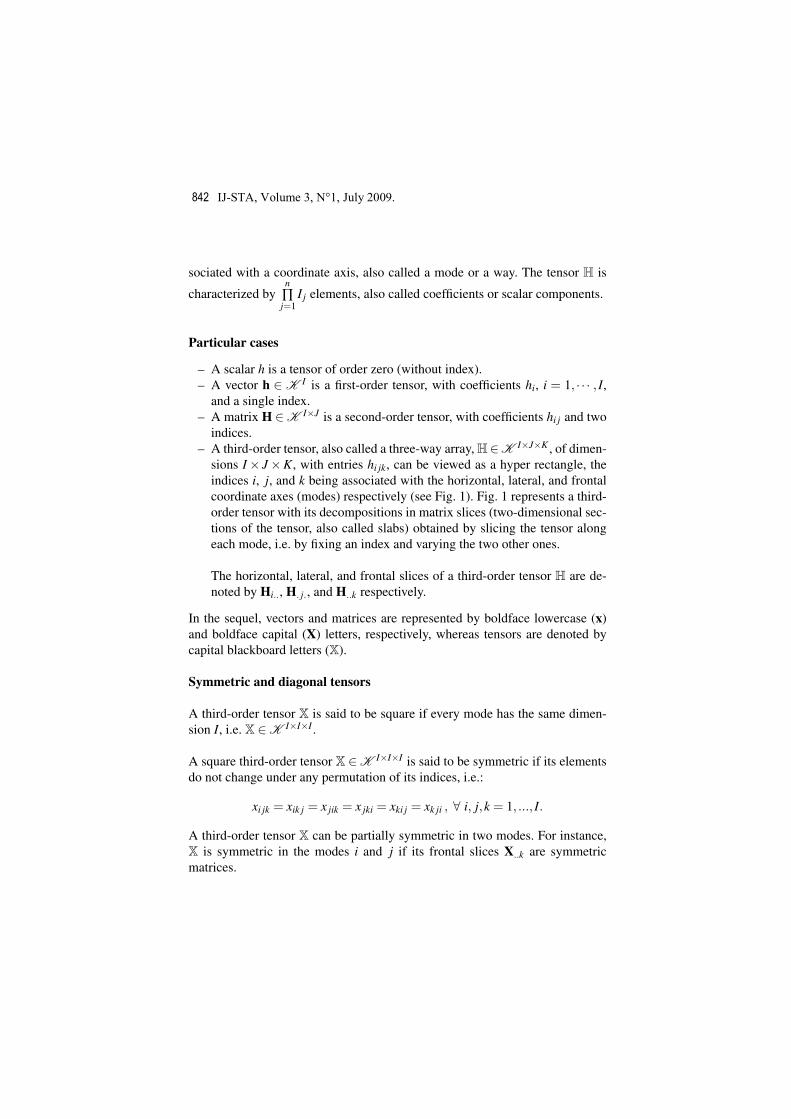
indices.– A third-order tensor, also called a three-way array,H∈K I×J×K , of dimen-

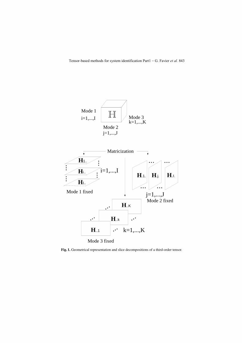
sions I× J×K, with entries hi jk, can be viewed as a hyper rectangle, theindices i, j, and k being associated with the horizontal, lateral, and frontalcoordinate axes (modes) respectively (see Fig. 1). Fig. 1 represents a third-order tensor with its decompositions in matrix slices (two-dimensional sec-tions of the tensor, also called slabs) obtained by slicing the tensor alongeach mode, i.e. by fixing an index and varying the two other ones.

The horizontal, lateral, and frontal slices of a third-order tensor H are de-noted by Hi.., H. j., and H..k respectively.

In the sequel, vectors and matrices are represented by boldface lowercase (x)and boldface capital (X) letters, respectively, whereas tensors are denoted bycapital blackboard letters (X).

Symmetric and diagonal tensors

A third-order tensor X is said to be square if every mode has the same dimen-sion I, i.e. X ∈K I×I×I .

A square third-order tensor X ∈K I×I×I is said to be symmetric if its elementsdo not change under any permutation of its indices, i.e.:

xi jk = xik j = x jik = x jki = xki j = xk ji , ∀ i, j,k = 1, ..., I.

A third-order tensor X can be partially symmetric in two modes. For instance,X is symmetric in the modes i and j if its frontal slices X..k are symmetricmatrices.

!"#$%"!&''(

4

Hi=1,...,I

j=1,...,J

k=1,...,KMode 3

Mode 2

Mode 1

......

H1..

Hi..

HI..

......

i=1,...,I......

H.1. H.j. H.J.

......

j=1,...,J

......

H..1

H..k

H..K

......

k=1,...,K

Matricization

Mode 1 fixed

Mode 2 fixed

Mode 3 fixed

Fig. 1. Geometrical representation and slice decompositions of a third-order tensor.

−#

5

A third-order tensor X is diagonal if xi jk 6= 0 only if i = j = k. The diagonaltensor with ones on its superdiagonal is called the identity tensor.

The above definitions can be easily extended to tensors of any order n > 3.

2 Examples of tensors in SP

2.1 Tensors of statistics

Third-order cumulants of three real vector random variables

Let x, y, and z be three real-valued vector random variables, of respective di-mensions M1, M2, and M3. The cumulant Cx,y,z = cum(x,y,z) is a third-ordertensor, with elements [Cx,y,z]m1,m2,m3

= cum(xm1 ,ym2 ,zm3). The modes 1, 2, and3 correspond to the components of each vector x, y, and z respectively.

Fourth-order cumulants of a real scalar stochastic process

Let x(k) be a discrete-time, stationary, real-valued, scalar stochastic process. Itsfourth-order cumulants define a third-order tensor, with entries [C4x]τ1,τ2,τ3

=cum(x(k),x(k− τ1),x(k− τ2),x(k− τ3)). The modes 1, 2, and 3 are associatedwith the time lags τ1, τ2, and τ3.

Spatio-temporal covariances of a real-valued vector stochastic process

Let x(t)∈ℜM be the vector of signals received on an M sensor array, at the timeinstant t. The spatio-temporal covariance matrices Cxx(k) = E

[x(t + k)xT (t)

],

k = 1, · · · ,K, define a third-order M×M×K tensor, with entries [Cxx]i, j,k =E [xi(t + k)x j(t)]. The two first modes i and j are spatial (sensor numbers)whereas the third mode k is temporal (covariance time lag).

Third-order space cumulants of a real-valued vector stochastic process

Let x(t) ∈ ℜM be the vector of signals received on an M sensor array, at thetime instant t. The third-order space cumulants cum(x,x,x) define a third-orderM×M×M tensor Cxxx, with elements [Cxxx]i, j,k = cum(xi(t),x j(t),xk(t)). Thethree modes i, j, and k are spatial, the signals being considered at the same timeinstant t.

!"#$%"!&''(

6

2.2 Kernels of Volterra models

SISO Volterra models

A P-th order Volterra model for a single-input single-output (SISO) system, isgiven by:

y(n) = h0 +P

∑p=1

Mp

∑m1=1

· · ·Mp

∑mp=1

hp(m1, · · · ,mp)p

∏j=1

u(n−m j)

where u(n) and y(n) denote respectively the input and output signals, P is thenonlinearity degree of the Volterra model, Mp is the memory of the pth-orderhomogeneous term, and hp(m1, · · · , mp) is a coefficient of the pth order kernel.This kernel can be viewed as an pth order Mp×Mp×·· ·×Mp tensor.

MIMO Volterra models

In the case of a multi-input multi-output (MIMO) Volterra model, with u(n) ∈ℜnI and y(n) ∈ℜnO , where nI and nO denote respectively the number of inputsand outputs, the input-output relationship, for s = 1, ...no, is given by:

ys(n) = hs0 +

P

∑p=1

nI

∑j1=1

· · ·nI

∑jp=1

Mp

∑m1=1

· · ·Mp

∑mp=1

hsj1,··· , jp(m1, · · · ,mp)

p

∏k=1

u jk(n−mk)

where hsj1,··· , jp

(m1, · · · ,mp) is the kernel of the sth output, acting on the productof p delayed input signals (with time delays m1, · · · , mp), these signals beingpossibly associated with different inputs ( j1, · · · , jp). This Volterra kernel isnow of order 2p and dimensions Mp×·· ·×Mp×nI ×·· ·×nI with p temporalmodes corresponding to the delays m1, · · · , mp and p space modes associatedwith inputs j1, · · · , jp.

2.3 Tensors of signals

Signals received by a communication system oversampled at the receiver

The signals received on an M antennas array, with an oversampling rate equalto P, and over a time duration of N symbol periods, constitute a tensor X ∈C M×N×P, with entries xm,n,p , m = 1, · · · ,M, n = 1, · · · ,N, p = 1, · · · ,P, thethree modes being associated with an antenna number (m), a symbol period (n),

−)

7

and an oversampling period (p).

Signals received by a CDMA (Code Division Multiple Access) system

At the transmitter, each symbol to be transmitted is spread by means of a spread-ing code of length J, with a period Tc = T/J, where T is the symbol period. So,each symbol is converted into J chips. A block of N signals received by M an-tennas can then be viewed as a third-order tensor X ∈ C M×N×J , with entriesxm,n, j, m = 1, · · · ,M, n = 1, · · · ,N, j = 1, · · · ,J.

Signals received by an OFDM (Orthogonal Frequency Division Multiplex-ing) system

In an OFDM system, the symbol sequence to be transmitted is organized intoblocks of F symbols in the frequency domain. In this case, the received signalsconstitute a third-order tensor X ∈ C M×N×F , with entries xm,n, f , m = 1, · · · ,M,n = 1, · · · ,N, f = 1, · · · ,F .

We can conclude that these three received signals have two modes in common(m and n), and differ from one another in the third mode (p, j, or f ). An unifiedtensor model of PARAFAC type was put in evidence for these three communi-cation systems [11].For illustrating these tensors of received signals, let us consider the case of aCDMA system [10]. In presence of Q users and in absence of noise, the signalreceived by the m-th antenna (m = 1, · · · ,M), at the n-th symbol period (n =1, · · · ,N), can be written as:

xm,n, j =Q

∑q=1

amqsnqc jq (1)

where amq denotes the fading coefficient of the channel between the q-th userand the m-th receive antenna, snq is the symbol transmitted by the q-th user, atthe n-th symbol period and using the j-th spreading code c jq. The set of sig-nals received by the M receive antennas, during N symbol periods and using Jspreading codes per user, constitutes a third-order tensor X ∈ C M×N×J . Equa-tion (1) corresponds to a PARAFAC model ( See Section 4.1).

!"#$%"!&''(

8

Xm=1,..., M

n=1,..., N

p=1,..., PMode 3

Mode 2

Mode 1

j=1,..., J

f=1,..., F

or

or

mn

p, j, or f

Fig. 2. Tensors of signals received by the three communication systems.

3 Some recalls on matrices and matrix decompositions

In this section, we recall some definitions relative to matrices and some matrixdecompositions.

For a matrix A ∈ C I×J , we denote by Ai. and A. j its i-th row vector and j-thcolumn vector respectively.

3.1 Column-rank and row-rank

For a matrix A∈ℜI×J , the number of linearly independent rows (columns) of Ais called the row-rank (column-rank) of A. The row-rank and the column-rankof a matrix are equal. This number, denoted by r(A), is called the rank of A.We have:

r(A)≤min(I,J)

– A is said to be full rank if r(A) = min(I,J) and rank-deficient if r(A) <min(I,J).

– A is said to be full column-rank if r(A) = J, i.e. if the J columns are inde-pendent.

−*

9

– Analogously, A is said to be full row-rank if r(A) = I, i.e. if the I rows areindependent.

For a square matrix A ∈ ℜI×I , if r(A) < I, then det(A) = 0 and A is calledsingular; if A is full-rank, then det(A) 6= 0 and A is called nonsingular.

For A ∈ℜI×J , we have:

r(AAT ) = r(AT A) = r(A)

For any full column-rank matrix C and full row-rank matrix B, with appropriatedimensions, we have :

r(A) = r(AB) = r(CA) = r(CAB).

3.2 The rank theorem

For any matrix A ∈ℜI×J , we have:

dimR(A)+dimN (A) = J

where R(A) = Ax/x ∈ℜJ is the column space, also called the range space,of A, and N (A) = x/Ax = 0 is the nullspace of A, with dimR(A) = r(A).From this theorem, we can conclude that:

– If A is full column-rank (dimR(A) = J), we have dimN (A) = 0 and con-sequently N (A) = 0.

– If A is rank-deficient (dimR(A) < J), we have dimN (A) > 0, which im-plies N (A) 6= 0.

3.3 k-rank (or Kruskal-rank)

The notion of k-rank was introduced by Kruskal [12] for studying the unique-ness of the PARAFAC decomposition of a given tensor.

Consider a matrix A ∈ ℜI×J of rank r(A). The k-rank of A is the largest inte-ger k such that any set of k columns of A is independent. It is denoted by kA.The k-rank is more constraining than the column-rank in the sense that kA = kmeans that any set of k columns of A is independent, whereas r(A) = k impliesthat there exists at least one set of k independent columns and any set of k + 1columns is dependent. So, we have: kA ≤ r(A).

!"#$%"!&''(

10

– If A ∈ℜI×J is full column-rank, then kA = J.– If A ∈ℜI×J has no all-zero column, but contains at least two proportional

columns, then kA = 1.– If A ∈ℜI×J has an all-zero column, then kA = 0.

Examples

A1 =

1 1 11 1 01 1 0

⇒ r(A1) = 2, kA1 = 1

A2 =

1 0 10 1 10 0 0

⇒ r(A2) = kA2 = 2

A3 =

1 0 00 1 00 0 0

⇒ r(A3) = 2, kA3 = 0

3.4 The vectorization operator vec(.)

The vec-operator put the matrix A ∈K I×J in the form of a column vector ofdimension IJ, denoted by vec(A), by stacking all the column vectors of A:

A =(A.1 · · · A.J

) ∈K I×J ⇒ vec(A) =

A.1...

A.J

∈K IJ

The matrix A is said to be vectorized, and we have:

v = vec(A)⇔ v(i−1)J+ j = ai j.

3.5 Kronecker and Khatri-Rao products

These matrix products are used for matricizing tensors.

The Kronecker product of two matrices A ∈K I×J and B ∈K K×L, denoted byA⊗B, is the partitioned matrix C ∈K IK×JL defined as:

C = A⊗B =

a11B a12B · · · a1JBa21B a22B · · · a2JB

......

. . ....

aI1B aI2B · · · aIJB

−(

11

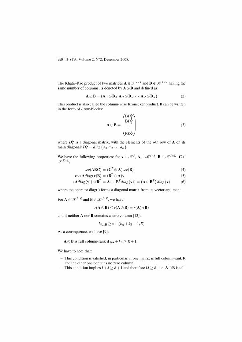
The Khatri-Rao product of two matrices A ∈K I×J and B ∈K K×J having thesame number of columns, is denoted by A¯B and defined as:

A¯B =(A.1⊗B.1 A.2⊗B.2 · · · A.J ⊗B.J

)(2)

This product is also called the column-wise Kronecker product. It can be writtenin the form of I row-blocks:

A¯B =

BDA1

BDA2

...BDA

I

(3)

where DAi is a diagonal matrix, with the elements of the i-th row of A on its

main diagonal: DAi = diag

(ai1 ai2 · · · aiJ

).

We have the following properties: for v ∈ K J , A ∈ K I×J , B ∈ K J×K , C ∈K K×L,

vec(ABC) = (CT ⊗A)vec(B) (4)vec(Adiag(v)B) = (BT ¯A)v (5)

(Adiag(v))¯BT = A¯ (BT diag(v)

)=

(A¯BT )

diag(v) (6)

where the operator diag(.) forms a diagonal matrix from its vector argument.

For A ∈K I×R and B ∈K J×R, we have:

r(A¯B)≤ r(A⊗B) = r(A)r(B)

and if neither A nor B contains a zero column [13]:

kA¯B ≥min(kA + kB−1,R)

As a consequence, we have [9]:

A¯B is full column-rank if kA + kB ≥ R+1.

We have to note that:

– This condition is satisfied, in particular, if one matrix is full column-rank Rand the other one contains no zero column.

– This condition implies I +J ≥ R+1 and therefore IJ ≥ R, i. e. A¯B is tall.

/ !"&$%&+&''

12

3.6 Moore-Penrose matrix pseudo-inverse

The Moore-Penrose pseudo-inverse of a matrix A ∈ K I×J is a J× I matrix,denoted by A†, that satisfies the four following conditions:

AA†A = A, A†AA† = A†, (AA†)T = AA†, (A†A)T = A†A.

The Moore-Penrose pseudo-inverse always exists and is unique. See its expres-sion in terms of the SVD in the next section.

If A ∈ C I×J is full column rank, its Moore-Penrose pseudo-inverse is given by:

A† = (AHA)−1AH .

The calculation of A† needs to inverse a J× J matrix.

If A is a nonsingular matrix, then A† = A−1.

3.7 Principal component analysis (PCA)

Consider a matrix A ∈ ℜI×J . If r(A) = R, then there exists a set of R pairs ofvectors

ur ∈ℜI ,vr ∈ℜJ ; r = 1, · · · ,R

such that:

A =R

∑r=1

urvTr (7)

or

A =R

∑r=1

ur vr

where the symbol denotes the vector outer product defined as follows:

ur ∈ℜI , vr ∈ℜJ ⇒ ur vr ∈ℜI×J ⇔ (ur vr)i j = uirv jr.

The scalar writing of this matrix decomposition is the following :

ai j =R

∑r=1

uirv jr, i = 1, · · · , I, j = 1, · · · ,J. (8)

This writing corresponds to a bilinear decomposition of A by means of R com-ponents, each term urvT

r , called a dyad, being a rank-one matrix. That means

−)

13

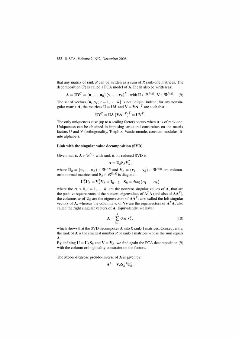
that any matrix of rank R can be written as a sum of R rank-one matrices. Thedecomposition (7) is called a PCA model of A. It can also be written as:

A = UVT =(u1 · · · uR

)(v1 · · · vR

)T, with U ∈ℜI×R, V ∈ℜJ×R. (9)

The set of vectors ur,vr; r = 1, · · · ,R is not unique. Indeed, for any nonsin-gular matrix ΛΛΛ , the matrices U = UΛΛΛ and V = VΛΛΛ−T are such that:

UVT = UΛΛΛ(VΛΛΛ−T )T = UVT .

The only uniqueness case (up to a scaling factor) occurs when A is of rank one.Uniqueness can be obtained in imposing structural constraints on the matrixfactors U and V (orthogonality, Toeplitz, Vandermonde, constant modulus, fi-nite alphabet).

Link with the singular value decomposition (SVD)

Given matrix A ∈ℜI×J with rank R, its reduced SVD is:

A = URSRVTR ,

where UR =(u1 · · · uR

) ∈ ℜI×R and VR =(v1 · · · vR

) ∈ ℜJ×R are column-orthonormal matrices and SR ∈ℜR×R is diagonal:

UTRUR = VT

RVR = IR ; SR = diag(σ1 · · · σR

)

where the σi > 0, i = 1, · · · ,R, are the nonzero singular values of A, that arethe positive square roots of the nonzero eigenvalues of AT A (and also of AAT ),the columns ui of UR are the eigenvectors of AAT , also called the left singularvectors of A, whereas the columns vi of VR are the eigenvectors of AT A, alsocalled the right singular vectors of A. Equivalently, we have:

A =R

∑r=1

σrurvTr , (10)

which shows that the SVD decomposes A into R rank-1 matrices. Consequently,the rank of A is the smallest number R of rank-1 matrices whose the sum equalsA.By defining U = URSR and V = VR, we find again the PCA decomposition (9)with the column orthogonality constraint on the factors.

The Moore-Penrose pseudo-inverse of A is given by:

A† = VRS−1R UT

R .

/ !"&$%&+&''

14

3.8 LS solutions of a set of linear equations

The least squares (LS) solutions of the set of linear equations Ax = y, withx ∈ ℜJ , y ∈ ℜI , A ∈ ℜI×J , are such that ‖Ax−y‖2

2 is minimized with respectto x. The LS solutions, denoted by xLS, are solutions of the normal equations:

AT AxLS = AT y.

It is important to mention that, even if the set of equations Ax = y is incon-sistent, i.e. it admits no exact solutions, which corresponds to y /∈ R(A), theset of normal equations AT Ax = AT y is always consistent, i.e. it always ad-mits at least one solution [14]. Indeed, AT y ∈R(AT ) = R(AT A) implies thatthe second member of the normal equations belongs to the column space of itscoefficient matrix (AT A), which is the condition to satisfy for ensuring the con-sistency of a system of linear equations.

The LS solution is unique if and only if A is full column-rank. In this case, wehave:

xLS = (AT A)−1AT y = A†y (11)

When A is rank-deficient, there exists an infinite number of LS solutions andthe general solution of the normal equations is given by:

xLS = A†y+(I−A†A)z (12)

where z is any vector of ℜJ . The second term of this sum belongs to thenullspace of A, which means R(I−A†A) = N (A). Indeed, we have:

A(I−A†A)z = (A−AA†A)z = 0

and consequently:

AT AxLS = AT A(A†y+

(I−A†A

)z)= AT AA†y = AT AA†Ax = AT Ax = AT y

which shows that xLS defined in (12) satisfies the normal equations.

We have to note that xLS = A†y is the LS solution of minimal Euclidean norm.

3.9 Low-rank approximation of a matrix using its SVD[15]

Let us consider a matrix A ∈ ℜI×J of rank R, admitting URSRVTR as reduced

SVD, with the singular values σ1 ≥ σ2 ≥ ·· · ≥ σR > σR+1 = · · ·= σmin(I,J) = 0

−)#

15

and denote by ‖A‖2F its Frobenius norm3. Its best rank-K approximation (K ≤

R), in the sense minB/r(B)=K

‖A−B‖2F , is given by the sum of the K rank-one ma-

trices of its SVD (10) associated with the K largest singular values:

AK =K

∑k=1

σkukvTk

and we have ‖A−AK‖2F =

R∑

k=K+1σ2

k .

This property is not valid for higher-order tensors.

4 Main tensor models

It is important to notice that, in SP applications, tensor models are generallydeduced from the underlying structure of the system under study and not fromalgebraic transforms applied to the data tensors. So, in the sequel, we will usethe terms tensor model (also called multiway model or multilinear model) in-stead of tensor decomposition.

We first present the most well-known and used tensor model, the so calledPARAFAC (Parallel Factor) model. Then, we will briefly describe several othertensor models (Tucker, PARATUCK2, CONFAC).

4.1 The PARAFAC model

The following decomposition of the third-order tensor X ∈ℜI×J×K :

xi jk =R

∑r=1

airb jrckr, i = 1, · · · , I, j = 1, · · · ,J, k = 1, · · · ,K, (13)

is called the PARAFAC decomposition ofX. Equation (13) is a generalization ofequation (8) to the third-order. It is a trilinear decomposition with R componentsthat can be also written as:

X=R

∑r=1

A.r B.r C.r, with A ∈ℜI×R, B ∈ℜJ×R, C ∈ℜK×R. (14)

3 The Frobenius norm of A ∈ℜI×J is defined as: ‖A‖2F = ∑

i, ja2

i j = trace(AT A).

/ !"&$%&+&''

16

Each term of the sum, called a triad, is a third-order rank-one tensor, i.e. theouter product of three vectors, also called an indecomposable tensor. So, PARAFACcorresponds to a decomposition of the tensor into a sum of R rank-one tensors.This is illustrated in Fig.3 .

=

A.1

B.1

C.1

A.R

B.R

C.R

XI

J

K ...+ +

Fig. 3. PARAFAC decomposition of a third-order tensor.

The column vectors A.r, B.r, and C.r are of respective dimensions I, J, and K.They contain the coefficients air, b jr, and ckr of the three matrix factors (alsocalled loadings or components) A, B, and C of the PARAFAC decomposition.

The PARAFAC model can be easily extended to any order N > 3:

xi1i2...iN =R

∑r=1

∏n

a(n)inr , in = 1, ..., In, n = 1, ...N, (15)

or equivalently

X=R

∑r=1

A(1).r A(2)

.r · · · A(N).r , with A(n) ∈ C In×R, n = 1, · · · ,N.

In certain applications, the matrix factors are used to interpret the underlyinginformation contained in the data tensors. In other applications, these factorscontain the information of interest on the system under study.

So, in wireless communication applications, tensors of transmitted and receivedsignals are decomposed into matrix factors that contain both the structure (de-sign) parameters and the information of interest on the communication system.

−))

17

For instance, with future multiuser MIMO systems where a base station willsimultaneously transmit data via multiple transmit antennas to several usersequipped with multiple receive antennas, tensor modeling can be used for blockspace-time spreading, i.e. each data stream is spread across both space (anten-nas) and time (symbols) dimensions [16]. In this case, the design parameterscorresponding to the tensor dimensions, are the number of transmit/receive an-tennas, the temporal spreading factor (number of spreading codes), the num-ber of data streams transmitted per block, and the number of symbol periods,whereas the information of interest to be recovered concerns the channel, thetransmitted symbols and eventually the spreading codes.

In the case of tensor-based blind identification methods for FIR linear systems,like the ones described in the second part of the paper, that are based on theuse of fourth-order output cumulants, the cumulant tensor admits a PARAFACmodel that is directly obtained from the transformation of the output signalsinto fourth-order cumulants.

In the same way, with the tensor-based approach for Wiener-Hammerstein non-linear system identification, the tensor corresponding to the third-order Volterrakernel associated with the Wiener-Hammerstein system to be identified, admitsa PARAFAC model that directly results from the underlying structure of theoriginal nonlinear system.

It is important to notice that the PARAFAC model captures the trilinear struc-ture in the data, but this model is linear in its parameters, i.e. the coefficients ofeach matrix factor. This property is exploited in the ALS algorithm for estimat-ing the PARAFAC parameters (see section 4.4).

In practice, a tensor of data is always represented as the sum of two terms : astructural term corresponding to the tensor model and a residual term containingboth the measurement noise and the modeling error, which means that (13) isin general replaced by:

xi jk =R

∑r=1

airb jrckr + ei jk, i =, · · · , I, j = 1, · · · ,J, k = 1, · · · ,K,

where ei jk denotes the components of the residual tensor E. An analysis of theseresiduals allows to quantify the fit of the tensor model with the data. The sumof squares of these residuals ( ‖E‖2

F = ∑i, j,k

e2i jk ) is often used as an objective

/ !"&$%&+&''

18

function for estimating the PARAFAC parameters, and as a test for stoping theALS algorithm.

Tensor rank

The rank of a third-order tensor X ∈ ℜI×J×K is the smallest number R of tri-linear factors in its PARAFAC decomposition, i.e. the smallest number R suchthat (13) is exactly satisfied.Other definitions exist for the rank of a tensor: symmetric rank, maximum rank,typical rank, generic rank.

Any symmetric tensor X ∈ C I×I×···×I of order N can be decomposed as a sumof R symmetric rank-1 tensors [17]:

X=R

∑r=1

A.r A.r · · · A.r, (16)

with the matrix factor A ∈ C I×R.

The symmetric rank (over C ) is defined as the minimum number R of symmet-ric rank-1 factors in the decomposition (16).

The maximum rank is defined as the largest achievable rank for a given setof tensors. For instance, the set of all third-order tensors X ∈ ℜI×J×K has amaximum rank, denoted by Rmax(I,J,K), such that [18]:

max(I,J,K)≤ Rmax(I,J,K)≤min(IJ, IK,JK).

Typical and generic ranks of tensors are more abstract concepts that are outsidethe scope of this paper ( See [19]).

Remarks

– Unlike matrices, the rank of a tensor can be larger than its largest dimen-sion, i.e. R can be larger than max(I,J,K).

– Kruskal [18] showed that the maximum possible rank of a third-order 2×2×2 tensor is equal to 3.

– The maximum possible rank of a third-order 3×3×3 tensor is equal to 5.– From a practical point of view, the rank of a tensor is difficult to determine.

−)*

19

Uniqueness properties

Uniqueness is a key property of the PARAFAC decomposition. Four kinds ofuniqueness can be defined [20]:

– Strict uniqueness: The matrix factors can be obtained without any ambigu-ity.

– Quasi-strict uniqueness: The matrix factors can be obtained up to columnscaling.

– Essential uniqueness: The matrix factors can be obtained up to column per-mutation and scaling.

– Partial uniqueness: One or two matrix factors are essentially unique, whilethe other(s) matrix factor(s) is (are) not.

Consider the third-order tensor X ∈ℜI×J×K . The PARAFAC decomposition ofX is said to be essentially unique if two sets of matrix factors (A,B,C) and (A,B, C) of the PARAFAC decomposition are linked by the following relations:

A = AΠ∆Π∆Π∆ 1, B = BΠ∆Π∆Π∆ 2, C = CΠ∆Π∆Π∆ 3,

where ΠΠΠ is a permutation matrix, and ∆∆∆ i = diag(di

11 · · · diRR

), i = 1,2,3, are

diagonal matrices such that:

∆∆∆ 1∆∆∆ 2∆∆∆ 3 = IR, i.e. d1rrd

2rrd

3rr = 1, r = 1, · · · ,R.

These permutation and scaling ambiguities are evident from the writings (13) or(14). The permutation matrix ΠΠΠ is associated with a reordering of the rank-onecomponent tensors, whereas the diagonal matrices ∆∆∆ i, i = 1,2,3, correspond toa scaling of the columns A.r, B.r, and C.r by the diagonal elements d1

rr , d2rr, and

d3rr respectively, so that the PARAFAC decomposition can be rewritten as:

X=R

∑r=1

(d1rrA.r) (d2

rrB.r) (d3rrC.r).

The first uniqueness results are due to Harshman [4, 21]. The most general suf-ficient condition for essential uniqueness is due to Kruskal [12, 18] and dependson the concept of k-rank.

/ !"&$%&+&''

20

Kruskal’s theorem

A sufficient condition for essential uniqueness of the PARAFAC decomposition(13), with (A, B, C) as matrix factors, is:

kA + kB + kC ≥ 2R+2. (17)

Remarks

– Condition (17) does not hold when R = 1. Uniqueness was proved byHarshman [21] in this particular case.

– Condition (17) is sufficient but not necessary for essential uniqueness. How-ever, it has recently been proved in [22] that (17) is also a necessary condi-tion for R = 2 and R = 3.

– Other sufficient uniqueness conditions for the case where one of the matrixfactors is full column rank are given in [23].

– The Kruskal’s condition was extended to complex-valued tensors in [10]and to N-way tensors (N>3) in [24]. The PARAFAC model (15) of order N,with matrix factors A(n), n = 1, · · · ,N, is essentially unique if:

∑n

kA(n) ≥ 2R+N−1.

4.2 Other third-order tensor models

Tucker models [2]

The Tucker model decomposes a tensor into a core tensor multiplied by a matrixalong each mode. For a third-order tensor X ∈ℜI×J×K , we have:

xi jk =P

∑p=1

Q

∑q=1

R

∑r=1

gpqraipb jqckr, i = 1, · · · , I, j = 1, · · · ,J, k = 1, · · · ,K. (18)

gpqr being an element of the third-order core tensor G ∈ℜP×Q×R.The Tucker model can also be written as :

X=P

∑p=1

Q

∑q=1

R

∑r=1

gpqrA.p B.q C.r

showing that X is decomposed into a weighted sum of PQR outer products,each weight corresponding to an element of the core tensor. This kind of tensor

−)(

21

model is more flexible due to the fact that it allows interactions between thedifferent matrix factors, the weights gpqr representing the amplitudes of theseinteractions.When P, Q , and R are smaller than I, J, and K, the core tensorG can be viewedas a compressed version of X.

The Tucker model can be viewed as the generalization of SVD to higher-ordertensors, and a Tucker model with orthogonal matrix factors is called an higher-order SVD (HOSVD) [25]. For an Nth-order tensor, the computation of itsHOSVD leads to the calculation of N matrix SVDs of unfolded matrices.

It is important to notice that the PARAFAC model with orthogonal matrix fac-tors occurs only if the tensor is diagonalizable, but, in general, tensors cannotbe diagonalized [26].

X = I

KP

Q

J

R

P

Q

R

A B

C

G

Fig. 4. Representation of the Tucker model for a third-order tensor.

The PARAFAC model is a special Tucker model corresponding to the casewhere P = Q = R and the core tensor is diagonal (gpqr = 1 if p = q = r and= 0 otherwise).

The Tucker model can be easily extended to any order N > 3:

xi1,··· ,iN =R1

∑r1=1

· · ·RN

∑rN=1

gr1,··· ,rN

N

∏j=1

ai jr j , i j = 1, · · · , I j, j = 1, · · · ,N.

From equation (18), it is possible to deduce two simplified Tucker models:

!"&$%&+&''

22

Tucker 2 model

xi jk =P

∑p=1

Q

∑q=1

hpqkaipb jq, i = 1, · · · , I, j = 1, · · · ,J, k = 1, · · · ,K. (19)

Comparing (19) with (18), we can conclude that a Tucker2 model is a Tuckermodel with one matrix factor equals to the identity matrix (C = IK) and R = K.

Tucker 1 model

xi jk =P

∑p=1

hp jkaip, i = 1, · · · , I, j = 1, · · · ,J, k = 1, · · · ,K. (20)

Tucker1 model is a Tucker model with B = IJ , C = IK , J = Q and R = K. Inthis case, two of the matrix factors are equal to the identity matrix.

It is important to notice that, unlike PARAFAC, Tucker models are not uniquein the sense that each matrix factor can be determined only up to a rotation ma-trix. Indeed, if a matrix factor is multiplied by a rotation matrix, application ofthe inverse of this rotation matrix to the core tensor gives the same tensor model.

PARATUCK2 model

The PARATUCK2 model of a third-order tensor X ∈ℜI×J×K is given by [27]:

xi jk =P

∑p=1

Q

∑q=1

aipcAkpgpqcB

kqb jq, i = 1, · · · , I, j = 1, · · · ,J, k = 1, · · · ,K. (21)

This model allows interactions between the columns of the matrix factors Aand B, along the third-mode, through the interaction matrices CA ∈ ℜK×P andCB ∈ℜK×Q, the matrix G ∈ℜP×Q defining the amplitude of these interactions.

The PARATUCK2 model was recently used for blind joint identification andequalization of Wiener-Hammerstein communication channels [28] and for space-time spreading-multiplexing in the context of MIMO wireless communicationsystems [29].

−,

23

CONFAC model

For a third-order tensor X ∈ℜI×J×K , the CONFAC model is given by [30]

xi jk =N

∑n=1

P

∑p=1

Q

∑q=1

R

∑r=1

g(n)pqraipb jqckr, i = 1, · · · , I, j = 1, · · · ,J, k = 1, · · · ,K.

(22)with N ≥max(P,Q,R) and g(n)

pqr = ψpnφqnωrn.The matricesΨΨΨ ∈ℜP×N , ΦΦΦ ∈ℜQ×N , and ΩΩΩ ∈ℜR×N , with respective elementsψpn, φqn, and ωrn, are called constraint matrices. They define the existence ornot of interaction (coupling) between the different modes.

X = I

K

G

P

Q

J

R

P

Q

R

A B

C

=ΨΨΨΨ.1

...ΦΦΦΦ.1ΨΨΨΨ.Ν

ΦΦΦΦ.Ν

ΩΩΩΩ.1 ΩΩΩΩ.Ν

G

+ +

Fig. 5. Representation of the CONFAC model for a third-order tensor.

The constraint matrices are chosen such that:

– Their elements ψpn, φqn, and ωrn are equal to 0 or 1, the value 1 implyingthe existence of an interaction whereas the value 0 implies no interaction.

– The columns of ΨΨΨ , ΦΦΦ , and ΩΩΩ , are canonical basis vectors of the Euclideanspaces ℜP , ℜQ, and ℜR respectively.

!"&$%&+&''

24

– ΨΨΨ , ΦΦΦ , and ΩΩΩ are full rank, which implies that each basis vector is containedat least once in each constraint matrix.

The CONFAC model illustrated in Fig. 5, can be viewed as a constrained Tuckermodel the core tensor of which admits a PARAFAC decomposition. Indeed,equation (22) is identical to (18) with: gpqr = ∑

ng(n)

pqr = ∑n

ψpnφqnωrn, which

corresponds to a PARAFAC model for the core tensor that depends on the con-straint matrices ΨΨΨ , ΦΦΦ , and ΩΩΩ .

The CONFAC model was used for designing new MIMO communication sys-tems [30]. Another constrained tensor model that can be viewed as a simplifiedversion of the CONFAC tensor model, is proposed in [31].

4.3 Matricization of a third-order tensorThe transformation that consists in putting a tensor of order larger than two un-der the form of a matrix is called matricization and the tensor is then said to bematricized.

Slice matrix representations

As illustrated in Fig. 1, a third-order I×J×K tensorH, with entries hi jk, can bematricized in matrix slices along each mode. Each matrix slice, denoted by Hi..,H. j., and H..k, contains the elements of a horizontal, lateral and frontal slice,respectively. These matrices can be explicited as follows:

Hi.. =

hi11 hi12 · · · hi1Khi21 hi22 · · · hi2K

......

. . ....

hiJ1 hiJ2 · · · hiJK

∈K J×K , H. j. =

h1 j1 h2 j1 · · · hI j1h1 j2 h2 j2 · · · hI j2

......

. . ....

h1 jK h2 jK · · · hI jK

∈K K×I

H..k =

h11k h12k · · · h1Jkh21k h22k · · · h2Jk

......

. . ....

hI1k hI2k · · · hIJk

∈K I×J .

In the case of the PARAFAC model with matrix factors (A, B, C), these matrixslices are given by:

Hi.. = BDAi CT , H. j. = CDB

j AT , H..k = ADCk BT , (23)

−,#

25

where DAi , DB

j , DCk are the following diagonal matrices of dimension R×R:

DAi = diag

(ai1 ai2 · · · aiR

)= diag(Ai.)

DBj = diag

(b j1 b j2 · · · b jR

)= diag(B j.)

DCk = diag

(ck1 ck2 · · · ckR

)= diag(Ck.)

Unfolded matrix representations

By stacking the matrices associated with a same type of slices, we get threedifferent unfolded matrix representations of the tensor H. These unfolded ma-trices, denoted by H1, H2, and H3, are defined as follows:

H1 =

H..1...

H..K

∈K IK×J , H2 =

H1.....

HI..

∈K JI×K , H3 =

H.1....

H.J.

∈K KJ×I .

(24)The three unfolded matrix representations of H are different from the point ofview of the organization of their elements but they are equivalent in terms ofinformation they contain since each one contains all the elements of the tensor.

In the case of the PARAFAC model, applying formula (3) to equations (23) and(24) leads to:

H1 = (C¯A)BT , H2 = (A¯B)CT , H3 = (B¯C)AT . (25)

Another way for unfolding the tensor consists in columnwise stacking the ma-trix slices, which leads to the following unfolded matrix representations:

H1 =(H..1 · · · H..K

)= A(C¯B)T ∈K I×JK ,

H2 =(H1.. · · · HI..

)= B(A¯C)T ∈K J×KI ,

H3 =(H.1. · · · H.J.

)= C(B¯A)T ∈K K×IJ .

In the case of the CONFAC model with matrix factors (A,B,C) and constraintmatrices (ΨΨΨ ,ΦΦΦ ,ΩΩΩ ), we have:

H1 =(CΩΩΩ¯AΨΨΨ)(BΦΦΦ)T , H2 =(AΨΨΨ¯BΦΦΦ)(CΩΩΩ)T , H3 =(BΦΦΦ¯CΩΩΩ)(AΨΨΨ)T .(26)

!"&$%&+&''

26

Comparing (26) with (25), we can conclude that the CONFAC model can beviewed as a constrained PARAFAC model in the sense that the factors (A,B,C)are replaced by the constrained factors (AΨΨΨ ,BΦΦΦ ,CΩΩΩ ). Indeed, (22) can berewritten as:

xi jk = ∑n

(∑p

aipψpn

)(∑q

b jqφqn

)(∑r

ckrωrn

)= ∑

n(AΨΨΨ)in(BΦΦΦ) jn(CΩΩΩ)kn,

which is a PARAFAC model with matrix factors (AΨΨΨ ,BΦΦΦ ,CΩΩΩ ).

4.4 Alternating Least Squares (ALS) algorithm

Identifying a PARAFAC model consists in estimating its matrix factors (A,B,C)from the knowledge of the data tensorH or equivalently its unfolded matrix rep-resentations. This parameter estimation problem can be solved in the LS sense,i.e. in minimizing the Frobenius norm of the residual tensor E, or equivalentlythe Frobenius norm of one of its unfolded matrices deduced from (25). So, forinstance, the LS cost function to be minimized can be written as :

minA,B,C

‖E3‖2F = min

A,B,C

∥∥H3− (B¯C)AT ∥∥2F (27)

The ALS algorithm originally proposed in [4] and [21], consists in replacing theminimization of the LS criterion (27) by an alternating minimization of threeconditional LS cost functions built from the three unfolded representations (25).Each cost function is minimized with respect to one matrix factor conditionallyto the knowledge of the two other matrix factors, this knowledge being providedfirst by the initialization and then by the estimates obtained at the previousiteration :

minA

∥∥H3− (Bt−1¯Ct−1)AT ∥∥2F ⇒ At

minB

∥∥H1− (Ct−1¯At)BT ∥∥2F ⇒ Bt

minC

∥∥H2− (At ¯Bt)CT ∥∥2F ⇒ Ct .

So, the initially trilinear LS problem that needs to use a nonlinear optimiza-tion method, is transformed into three linear LS problems that are successivelysolved by means of the standard LS solution. As we recalled in Section 3.8,these three LS problems admit an unique solution if anf only if A¯B, B¯C,

−,)

27

and C¯A are full column-rank, which directly leads to the following LS solu-tion uniqueness condition [32]:

minr(A¯B),r(B¯C),r(C¯A= R.

We have to note that the sufficient Kruskal’s condition (17) implies the abovecondition.

The ALS algorithm is summarized as follows:

1. Initialize B0 and C0 and set t = 0.2. Increment t and compute:

(a) At =((Bt−1¯Ct−1)

† H3

)T.

(b) Bt =((Ct−1¯At)

† H1

)T.

(c) Ct =((At ¯Bt)

† H2

)T.

3. Return to step 2 until convergence.

So, ALS is an iterative algorithm that successively estimates, at each iteration,one matrix factor in keeping the two other ones fixed to their previous esti-mated value. The computation loop is repeated until a convergence test is satis-fied. This test is built either from the estimated parameters, or using a criterionbased on the tensor reconstructed with the estimated parameters. It generallyconsists in detecting if an estimated parameter variation between two consec-utive iterations or a model fit error becomes smaller than a predefined threshold.

The ALS algorithm can be easily extended to both higher-order PARAFACmodels and to Tucker models with orthogonality constraints on the matrix fac-tors.

The main advantage of the ALS algorithm is its simplicity. However, its con-vergence can be very slow and convergence towards the global minimum is notguaranteed. That is much depending on the initialization. Different solutionsexist for improving the ALS algorithm in terms of speed of convergence andstability [33–35].

5 Conclusion

In this first part of the paper, the main definitions and properties relative to ten-sors have first been recalled before giving a brief review of the most used tensor

!"&$%&+&''

28

models. Some examples of tensors encountered in SP have been described forsignal and system modeling.Tensors constitute a very interesting research area, with very promising applica-tions in various domains. However, fundamental properties of tensors in termsof rank and uniqueness remain to be better understood. New tensor models andtensor decompositions are to be studied, and more robust parameter estimationalgorithms are necessary to render tensor-based SP methods even more effi-cient and attractive. Low-rank approximation of tensors of rank larger than oneis also a very important open problem with the objective of tensor dimension-ality reduction, which is very useful for tensor object feature extraction andclassification. More generally, tensor simplification, like diagonalization for in-stance, by means of transforms, is also an open issue. Finally, other applicationsof tensor tools can be considered as, for instance, for multidimensional filteringwith application to noise reduction in color images and seismic data [36] andalso to channel equalization.In the second part of this paper, we present three examples of tensor-basedmethods for system identification.

References

1. Hitchcock, F.: The expression of a tensor or a polyadic as a sum of products. J.Math. Phys. Camb. 6 (1927) 164–189

2. Tucker, L.: Some mathematical notes of three-mode factor analysis. Psychometrika31(3) (1966) 279–311

3. Caroll, J., Chang, J.: Analysis of individual differences in multidimensional scalingvia an N-way generalization of "Eckart-Young" decomposition. Psychometrika 35(1970) 283–319

4. Harshman, R.: Foundation of the PARAFAC procedure: models and conditions foran "explanatory" multimodal factor analysis. UCLA working papers in phonetics16 (1970) 1–84

5. Bro, R.: PARAFAC. Tutorial and applications. Chemometrics and Intelligent Lab-oratory Systems 38 (1997) 149–171

6. Cardoso, J.F.: Eigen-structure of the fourth-order cumulant tensor with applicationto the blind source separation problem. In: Proc. Int. Conf. on Acoustics, Speech,and Signal Processing (ICASSP), Albuquerque, New Mexico, USA (1990) 2655–2658

7. Cardoso, J.F.: Super-symmetric decomposition of the fourth-order cumulant tensor.Blind identification of more sources than sensors. In: Proc. Int. Conf. on Acoustics,Speech, and Signal Processing (ICASSP), Toronto, Ontario, Canada, (1991) 3109–3112

−,*

29

8. McCullagh, P.: Tensor methods in statistics. Chapman and Hall (1987)9. Sidiropoulos, N., Bro, R., Giannakis, G.: Parallel factor analysis in sensor array

processing. IEEE Trans. on Signal Processing 48(8) (2000) 2377–238810. Sidiropoulos, N., Giannakis, G., Bro, R.: Blind PARAFAC receivers for DS-CDMA

systems. IEEE Trans. on Signal Processing 48(3) (2000) 810–82311. de Almeida, A.L.F., Favier, G., Mota, J.C.M.: PARAFAC-based unified tensor mod-

eling for wireless communication systems with application to blind multiuser equal-ization. Signal Processing 87(2) (2007) 337–351

12. Kruskal, J.: Three-way arrays: rank and uniqueness of trilinear decompositions,with application to arithmetic complexity and statistics. Linear Algebra Applicat.18 (1977) 95–138

13. Sidiropoulos, N., Liu, X.: Identifiability results for blind beamforming in incoherentmultipath with small delay spread. IEEE Trans. on Signal Processing 49(1) (2001)228–236

14. Meyer, C.: Matrix analysis and applied linear algebra. SIAM (2000)15. Eckart, C., Young, G.: The approximation of one matrix by another of lower rank.

Psychometrika 1 (1936) 211–21816. de Almeida, A.L.F., Favier, G., Mota, J.C.M.: Multiuser MIMO system using block

space-time spreading and tensor modeling. Signal Processing 88(10) (2008) 2388–2402

17. Comon, P., Golub, G., Lim, L.H., Mourrain, B.: Symmetric tensors and symmetrictensor ranks. SCCM technical report 06-02, Stanford University (2006)

18. Kruskal, J.: Rank, decomposition and uniqueness for 3-way and n-way arrays. InCoppi, R., Bolasco, S., eds.: Multiway data analysis. Elsevier, Amsterdam (1989)8–18

19. Comon, P., ten Berge, J.: Generic and typical ranks of three-way arrays. Technicalreport, I3S (2006)

20. Kibangou, A., Favier, G.: Blind equalization of nonlinear channels using tensordecompositions with code/space/time diversities. Signal Processing 89(2) (2009)133–143

21. Harshman, R.: Determination and proof of minimum uniqueness conditions forPARAFAC 1. UCLA working papers in phonetics 22 (1972) 111–117

22. ten Berge, J., Sidiropoulos, N.: On uniqueness in CANDECOMP/PARAFAC. Psy-chometrika 67(3) (2002) 399–409

23. Jiang, T., Sidiropoulos, N.: Kruskal’s permutation lemma and the identification ofCANDECOMP/PARAFAC and bilinear models with constant modulus constraints.IEEE Trans. on Signal Processing 52(9) (2004) 2625–2636

24. Sidiropoulos, N., Bro, R.: On the uniqueness of multilinear decomposition of n-wayarrays. Journal of Chemometrics 14 (2000) 229–239

25. De Lathauwer, L., De Moor, B., Vandevalle, J.: A multilinear singular value decom-position. SIAM J. Matrix Anal. Appl. 21 (2000) 1253–1278

26. Kolda, T.: Orthogonal tensor decompositions. SIAM J. Matrix Anal. Appl. 23(1)(2001) 243–255

!"&$%&+&''

30

27. Harshman, R., Lundy, M.: Uniqueness proof for a family of models sharing featuresof Tucker’s three-mode factor analysis and PARAFAC/CANDECOMP. Psychome-trika 61(1) (1996) 133–154

28. Kibangou, A., Favier, G.: Blind joint identification and equalization of Wiener-Hammerstein communication channels using PARATUCK-2 tensor decomposition.In: Proc. EUSIPCO, Poznan, Poland (2007)

29. de Almeida, A.L.F., Favier, G., Mota, J.C.M.: Space-time spreading-multiplexingfor MIMO antenna systems using the PARATUCK2 tensor decomposition. In:Proc. EUSIPCO, Lausanne, Switzerland (2008)

30. de Almeida, A.L.F., Favier, G., Mota, J.C.M.: A constrained factor decompositionwith application to MIMO antenna systems. IEEE Trans. on Signal Processing 56(6)(2008) 2429–2442

31. de Almeida, A.L.F., Favier, G., Mota, J.C.M.: Constrained tensor modeling ap-proach to blind multiple-antenna CDMA schemes. IEEE Trans. on Signal Process-ing 56(6) (2008) 2417–2428

32. Liu, X., Sidiropoulos, N.: Cramer-Rao lower bounds for low-rank decompositionof multidimensional arrays. IEEE Trans. on Signal Processing 49(9) (2001) 2074–2086

33. Bro, R.: Multi-way analysis in the food industry. Models, algorithms and applica-tions. PhD thesis, University of Amsterdam, Netherlands (1998)

34. Tomasi, G., Bro, R.: A comparison of algorithms for fitting the PARAFAC model.Comp. Stat. Data Anal. 50(7) (2006) 1700–1734

35. Rajih, M., Comon, P., Harshman, R.: Enhanced line search : a novel method toaccelerate PARAFAC. (SIAM J. Matrix Anal. (To appear))

36. Muti, D., Bourennane, S.: Survey on tensor signal algebraic filtering. Signal Pro-cessing 87(2) (2007) 237–249

−,(