``Tensor products'' between metric spaces and Banach spaces

“Tensor products” between metric spaces andBanach spaces

J. Alejandro Chávez-Domínguez

Department of MathematicsTexas A&M University

BIRSMarch 8th, 2012

Algebraic tensor products

Tensor products are normally used to linearize bilinear maps.

E × F

��

ϕ // G

E ⊗ F

ϕ̃<<y

yy

yy

What sense could there possibly be in thinking about tensorproducts of a metric space with a Banach space?

Tensor products and Banach spaces

In Banach space theory, tensor products are used for morethan linearizing bilinear maps.

There are many different choices for a “reasonable” norm onE ⊗ F.

Most importantly, there are deep connections between tensornorms and operator ideals.

Duality relations

It often happens that

(E ⊗α F)∗ ≡ A(E,F∗)

for some tensor norm α and some operator ideal A.

Examples:1 (E ⊗π F)∗ ≡ L(E,F∗).

2 (E ⊗dp F)∗ ≡ Πp′(E,F∗).

3 (E ⊗w2 F)∗ ≡ Γ2(E,F∗).

All of these examples have nonlinear counterparts.

Tensoring with the identity

Another type of result takes the form

T ∈ A(E,F) ⇔ ‖T ⊗ idG : E ⊗α G→ F ⊗β G‖ <∞ ∀G.

with A an operator ideal and α, β tensor norms.Examples:

1 T ∈ Πp(E,F)⇔∥∥∥T ⊗ idG : E ⊗dp′ G→ F ⊗d1 G

∥∥∥ <∞∀G.

2 T ∈ Mq,p(E,F)⇔∥∥∥T ⊗ idG : E ⊗dp′ G→ F ⊗dq′ G

∥∥∥ <∞∀G.

Again, these and other examples have nonlinear counterparts.

Duality results

A baby example for duality

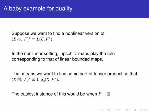
Suppose we want to find a nonlinear version of(E ⊗π F)∗ ≡ L(E,F∗).

In the nonlinear setting, Lipschitz maps play the rolecorresponding to that of linear bounded maps.

That means we want to find some sort of tensor product so that(X �π F)∗ ≡ Lip0(X,F∗).

The easiest instance of this would be when F = R.

The Arens-Eells space

The Arens-Eells space of a metric space X (denoted Æ(X)),also known as the free Lipschitz space of X (denoted F (X))satisfies

F (X)∗ ≡ X# := Lip0(X,R) = {f : X → R : Lip(f ) <∞, f (0) = 0}.

It was introduced in [Arens/Eells 1956], and has been used inBanach space theory [Godefroy/Kalton 2003], [Kalton 2004].

Molecules and the Arens-Eells space

A molecule on a metric space X is a finitely supportedm : X → R such that ∑

x∈X

m(x) = 0.

Note that the space of molecules is a vector space.Those of the form amxx′ where

mxx′ := χ{x} − χ{x′}

with a ∈ R and x, x′ ∈ X are called atoms.The Arens-Eells space of X is the space of molecules withthe norm

‖m‖F (X) := inf{ n∑

j=1

|aj|d(xj, x′j) : m =

n∑j=1

ajmxjx′j

}.

Properties of the Arens-Eells space

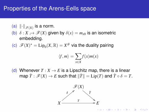
(a) ‖·‖F (X) is a norm.(b) δ : X ↪→ F (X) given by δ(x) = mx0 is an isometric

embedding.(c) F (X)∗ = Lip0(X,R) = X# via the duality pairing

〈f ,m〉 =∑x∈X

f (x)m(x)

(d) Whenever T : X → E is a Lipschitz map, there is a linearmap T̂ : F (X)→ E such that ‖T̂‖ = Lip(T) and T̂ ◦ δ = T.

F (X)

T̂

""DDDDDDDD

X

δ<<zzzzzzzz T // E

Duality for L(E,F)

Theorem

(E ⊗π F)∗ = L(E,F∗).

Where for w ∈ E ⊗ F

‖w‖π = inf

n∑

j=1

‖uj‖ · ‖vj‖ : w =

n∑j=1

uj ⊗ vj

and the identification is given via trace duality, considering anelement in E ⊗ F as a map F∗ → E. That is, forw =

∑nj=1 uj ⊗ vj ∈ E ⊗ F and T : E → F∗,

〈T,w〉 = tr(w ◦ T) =

n∑j=1

〈Txj, yj〉.

Vector valued molecules

Definition (C, 2011)

Let X be a metric space and E a Banach space.An E-valued molecule on X is a function m : X → E such that∑

x∈X

m(x) = 0.

An E-valued atom is a function of the form vmxx′ withx, x′ ∈ X and v in E.Every E-valued molecule on X can be expressed as a sumof E-valued atoms.

Projective norm for vector valued molecules

For an E-valued molecule m, let

‖m‖π := inf{ n∑

j=1

‖vj‖ d(xj, x′j) : m =

n∑j=1

vjmxjx′j

}.

We will denote by X �π E the space of E-valued molecules on Xwith the projective norm. It is not hard to show that

(X �π E)∗ = Lip0(X,E∗)

with the duality given by the pointwise pairing

〈T,m〉 =∑x∈X

〈T(x),m(x)〉.

It was known that Lip0(X,E∗) is a dual space [J. Johnson,1970], but as far as I know the approach via molecules is new.

“Products” of operators

Proposition (C, 2012)

Let S : X → Z be a Lipschitz map mapping 0 to 0, and T : E → Fa bounded linear map. Then there is a unique operatorS � T : X �π E → Z �π F such that

(S � T)(vmxy) = (Tv)m(Sx)(Sy), for all v ∈ E, x, y ∈ X.

Furthermore, ‖S �π T‖ = Lip(S) ‖T‖.

Justifying the “projective” name

Recall that a linear operator T : E → F is a linear quotient if it issurjective and

‖w‖ = inf{‖v‖ : v ∈ E, Tv = w

}for every w ∈ F.

On the other hand, a map S : X → Z is called a C-co-Lipschitz iffor every x ∈ X and r > 0,

f(B(x, r)

)⊇ B

(f (x), r/C

).

A map that is Lipschitz, co-Lipschitz and surjective is aLipschitz quotient.

Theorem (C, 2012)

Let S : X → Z be a Lipschitz quotient with Lipschitz andco-Lipschitz constants equal to 1, and mapping 0 to 0, and letT : E → F be a linear quotient map. ThenS �π T : (X �π E)→ (Z �π F) is also a linear quotient map.

Example: X = a graph-theoretic tree

Recall

‖m‖π = inf{ n∑

j=1

‖vj‖ d(xj, x′j) : m =

n∑j=1

vjmxjx′j

}

Note we can consider only representations where the pairs(xj, x′j) are endpoints of edges. Since X is a tree, everymolecule has only one such representation so

X �π E ≡ `N1 (E)

where N = # of edges of X.I suspect a similar result should work for more general metrictrees as in [Godard 2010].

Reasonable tensor norms

A tensor norm α is called reasonable if it satisfies(a) α(u⊗ v) ≤ ‖u‖ · ‖v‖ for every u ∈ E, v ∈ F.(b) α∗(u∗ ⊗ v∗) ≤ ‖u∗‖ ‖v∗‖ for every u∗ ∈ E∗, v∗ ∈ F∗.

Reasonable tensor norms are characterized by being betweenthe projective and injective tensor norms: a tensor norm α isreasonable if and only if ε ≤ α ≤ π, where

‖w‖ε = sup

n∑

j=1

〈u∗, uj〉〈v∗, vj〉 : w =

n∑j=1

uj ⊗ vj, u∗ ∈ BE∗ , v∗ ∈ B∗F

.

Reasonable molecular norms

A norm ‖·‖ on the space of E-valued molecules on a metricspace X is called reasonable if

(i) ‖vmxx′‖ ≤ ‖v‖ d(x, x′) for all x, x′ ∈ X, v ∈ E.(ii) |〈v∗ ◦ m, f 〉| ≤ ‖v∗‖Lip(f ) ‖m‖ for all v∗ ∈ E∗, m ∈M(X,E)

and f ∈ X#.Reasonable molecular norms are also characterized by beingbetween the projective and injective norms: a molecular norm αis reasonable if and only if ε ≤ α ≤ π, where

‖m‖ε = sup{ n∑

j=1

[f (xj)− f (x′j)

]v∗(vj)

: m =

n∑j=1

vjmxjx′j, f ∈ BX# , v∗ ∈ BE∗

}.

The injective norm

The injective norm is also deserving of its name: it behaveswell under injections.

However, it is not so interesting for us because it “forgets” aboutthe metric space and only takes into account the structure ofF (X). In fact,

X �ε E ≡ F (X)⊗ε E.

p-summing operators

E, F Banach spaces, T : E → F a linear map, 1 ≤ p ≤ ∞.

T is called p-summing if there exists C > 0 such that for anyv1, . . . vn in E we have n∑

j=1

‖Tvj‖p

1/p

≤ C supφ∈BE∗

n∑j=1

|φ(vj)|p1/p

.

The p-summing norm of T is

πp(T) := inf C.

The space of p-summing operators from E to F is denoted

Πp(E,F).

Chevet-Saphar norms

Theorem (Saphar 1970)

(E ⊗dp F

)∗= Πp′(E,F∗).

Where

Definition (Chevet 1969, Saphar 1965,1970)

For 1 ≤ p ≤ ∞ and w ∈ E ⊗ F, define p′ by 1/p + 1/p′ = 1 and

‖w‖dp:= inf

{supφ∈BE∗

[ n∑j=1

|φ(uj)|p′]1/p′

·[ n∑

j=1

‖vj‖p]1/p

: w =

n∑j=1

uj ⊗ vj

}.

p-summing operators

Definition (Pietsch, 1966)

E, F Banach spaces , T : E → F a linear map , 1 ≤ p ≤ ∞.


j=1

‖Tvj‖p

1/p

≤ C supφ∈BE∗

n∑j=1

|φ(vj)|p1/p


πp(T) := inf C.

Lipschitz p-summing operators

Definition (Farmer/Johnson, 2009)



j=1

‖Tvj‖p

1/p

≤ C supφ∈BE∗

n∑j=1

|φ(vj)|p1/p


πp(T) := inf C.





j=1

‖Tvj‖p

1/p

≤ C supφ∈BE∗

n∑j=1

|φ(vj)|p1/p


πp(T) := inf C.



X, Y metric spaces , T : E → F a linear map , 1 ≤ p ≤ ∞.


j=1

‖Tvj‖p

1/p

≤ C supφ∈BE∗

n∑j=1

|φ(vj)|p1/p


πp(T) := inf C.



X, Y metric spaces , T : E → F a linear map , 1 ≤ p ≤ ∞.


j=1

‖Tvj‖p

1/p

≤ C supφ∈BE∗

n∑j=1

|φ(vj)|p1/p


πp(T) := inf C.



X, Y metric spaces , T : X → Y a Lipschitz map , 1 ≤ p ≤ ∞.


j=1

‖Tvj‖p

1/p

≤ C supφ∈BE∗

n∑j=1

|φ(vj)|p1/p


πp(T) := inf C.





j=1

‖Tvj‖p

1/p

≤ C supφ∈BE∗

n∑j=1

|φ(vj)|p1/p


πp(T) := inf C.




T is called Lipschitz p-summing if there exists C > 0 such thatfor any v1, . . . vn in E we have n∑

j=1

‖Tvj‖p

1/p

≤ C supφ∈BE∗

n∑j=1

|φ(vj)|p1/p


πp(T) := inf C.




T is called Lipschitz p-summing if there exists C > 0 such thatfor any v1, . . . vn in E we have n∑

j=1

‖Tvj‖p

1/p

≤ C supφ∈BE∗

n∑j=1

|φ(vj)|p1/p


πp(T) := inf C.




T is called Lipschitz p-summing if there exists C > 0 such thatfor any x1, . . . xn, x′1, . . . x

′n in X we have n∑

j=1

‖Tvj‖p

1/p

≤ C supφ∈BE∗

n∑j=1

|φ(vj)|p1/p


πp(T) := inf C.






j=1

‖Tvj‖p

1/p

≤ C supφ∈BE∗

n∑j=1

|φ(vj)|p1/p


πp(T) := inf C.






j=1

d(Txj,Tx′j)p

1/p

≤ C supφ∈BE∗

n∑j=1

|φ(vj)|p1/p


πp(T) := inf C.






j=1

d(Txj,Tx′j)p

1/p

≤ C supφ∈BE∗

n∑j=1

|φ(vj)|p1/p


πp(T) := inf C.






j=1

d(Txj,Tx′j)p

1/p

≤ C supf∈BX#

n∑j=1

∣∣f (xj)− f (x′j)∣∣p1/p


πp(T) := inf C.






j=1

d(Txj,Tx′j)p

1/p

≤ C supf∈BX#

n∑j=1

∣∣f (xj)− f (x′j)∣∣p1/p


πp(T) := inf C.






j=1

d(Txj,Tx′j)p

1/p

≤ C supf∈BX#

n∑j=1

∣∣f (xj)− f (x′j)∣∣p1/p

The Lipschitz p-summing norm of T is

πLp (T) := inf C.

Duality for Lipschitz p-summing operators

Theorem (C 2011)

(X �dp F

)∗= ΠL

p′(X,F∗).

Where ΠLp denotes the Lipschitz p-summing operators of

[Farmer/Johnson 2009] and

Definition (C 2011)

For an E-valued molecule m on a metric space X,

‖m‖dp= inf

{(∑j

λpj ‖vj‖p

)1/psup

f∈BX#

(λ−p′

j |f (xj)− f (x′j)|p′)1/p′

: m =∑

j

vjmxjx′j, λj > 0

}.

Linear factorization through Hilbert space

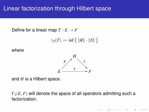
Define for a linear map T : E → F

γ2(T) := inf{‖R‖ · ‖S‖

}where

HS

��@@@

@@@@

E

R??~~~~~~~ T // F

and H is a Hilbert space.

Γ2(E,F) will denote the space of all operators admitting such afactorization.

Duality for Γ2(E,F)

Theorem

(E ⊗w2 F)∗ = Γ2(E,F∗)

Where for w ∈ E ⊗ F

‖u‖w2= inf

{( n∑j=1

‖uj‖2)1/2( n∑

i=1

‖vi‖2)1/2

:

u =∑

ij

aijuj ⊗ vi, ‖(aij) : `n2 → `n

2‖ ≤ 1}

and the identification is given again via trace duality.

Lipschitz factorization through subsets of Hilbert space

Define for a Lipschitz map T : X → Y

γLip2 (T) := inf

{Lip(R) · Lip(S)

}where

ZS

��???

????

X

R??�� T // Y

and Z is a subset of a Hilbert space.

Duality for ΓLip2

The norm on molecules that gives the duality for ΓLip2 is

‖m‖w2= inf

{( n∑i=1

‖vi‖2)1/2( m∑

j=1

d(x,x′j)2)1/2

:

m =

n∑i=1

vimyiy′i, myiy′i

=

m∑j=1

aijmxjx′j, ‖(aij) : `m

2 → `n2‖ ≤ 1

}

Tensoring with the identity

Representation theorems

Operator ideals satisfying certain technical properties can becharacterized by theorems of the following form:

Representation theorem

A linear operator T : E → F belongs to the operator ideal A ifand only if for every Banach space G, the map

T ⊗ idG : E ⊗α G→ F ⊗β G

is continuous.

Here, α and β are certain tensor norms.

Example

A linear operator T : E → F is p-summing if and only if for everyBanach space G the map

T ⊗ idG : E ⊗dp′ G→ F ⊗π G

is continuous.

Moreover, in this case

πp(T) = infG‖T ⊗ idG‖

A nonlinear version

Theorem (C, 2011)

TFAE:(a) T : X → Y is Lipschitz p-summing.(b) For every Banach space E (or only E = Y#),∥∥∥T � idE : X �d′p E → Y �π E

∥∥∥ <∞

(q, p)-mixing operators

Theorem

Let T : E → F be a linear map, 1 ≤ p ≤ q ≤ ∞. TFAE:(a) ∃ C > 0 such that for every S : F → G,

πp(S ◦ T) ≤ Cπq(S).

(b) For every Banach space G (or only G = `q′),∥∥∥T ⊗ idG : E ⊗dp′ G→ F ⊗dq′ G∥∥∥ <∞

Similarly

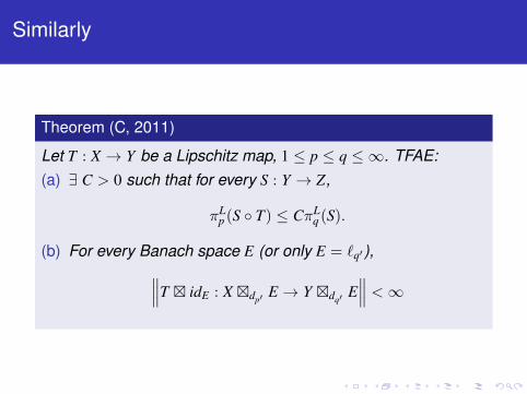
Theorem (C, 2011)

Let T : X → Y be a Lipschitz map, 1 ≤ p ≤ q ≤ ∞. TFAE:(a) ∃ C > 0 such that for every S : Y → Z,

πLp (S ◦ T) ≤ CπL

q (S).

(b) For every Banach space E (or only E = `q′),∥∥∥T � idE : X �dp′ E → Y �dq′ E∥∥∥ <∞

Date post:	12-Feb-2022
Category:	Documents
Upload:	others
View:	7 times
Download:	0 times

``Tensor products'' between metric spaces and Banach spaces

Documents