TENSOR PRODUCTS OF SPACES OF MEASURES ANDVECTOR INTEGRATION IN TENSOR PRODUCT SPACES

by

Donald P. Story

A DISSERTATION PRESENTED TO THE GRADUATE COUNCIL OF THEUNIVERSITY OF FLORIDA IN PARTIAL FULFILLMENT OF THE

REQUIREMENTS FOR THE DEGREE OFDOCTOR OF PHILOSOPHY

UNIVERSITY OF FLORIDA

1974

To my Parents

Whose faith in me never waivered,

ACKNOWLEDGMENTS

I would like to thank Kira whose encouragement during

the past two years has given me strength. I am indebted to

each member of my committee; special thanks are due to Dr.

James K. Brooks, who directed my research and guided my studies

in measure and integration theory, and to Dr. Steve Saxon for

his summer seminars on topological vector spaces. Finally,

I would like to thank Brenda Hobby for her excellent typing

job.

TABLE OF CONTENTS

Page

Acknowledgments iii

Abstract v

Introduction 1

Chapter

I. Tensor Products of Vector Measures 4

II. Tensor Products of Spaces of Measures 16

III. Pettis and Lebesgue Type Spaces andVector Integration 46

IV. The Fubini Theorem 88

Bibliography 112

Biographical Sketch 114

Abstract of Dissertation Presented to the GraduateCouncil of the University of Florida in Partial Fulfillmentof the Requirements for the Degree of Doctor of Philosophy

TENSOR PRODUCTS OF SPACES OF MEASURES ANDVECTOR INTEGRATION IN TENSOR PRODUCT SPACES

By

Donald P. Story

August, 1974

Chairman: J. K- BrooksMajor Department: Department of Mathematics

This dissertation investigates the concepts of measure

and integration within the framework of the topological tensor

product of two Banach spaces. In Chapter I, basic existence

theorems are given for the tensor product of two vector measures.

The topological tensor product of certain spaces of measures

is studied in Chapter II, where the space of all measures with

the Radon-Nikodym Property and the space of all measures with

relatively norm compact range are identified in terms of tensor

products. Chapter III discusses the theory of integration of

vector valued functions with respect to a vector measure; the

value of the integral is in the inductive tensor product of

the range spaces, and the integral is a generalization of B. J.

Pettis' weak integral. Normed Pettis and Bochner-Lebesgue

spaces are considered and the Vitali and Lebesgue Dominated

Convergence theorems are proved. Finally, in Chapter IV, the

integration theory of Chapter III is used with the product

measures discussed in Chapter I and II, to prove some Fubini

theorems for product integration.

INTRODUCTION

This dissertation concerns the topological tensor product

of certain spaces of measures, and integration theory for vector

valued functions with respect to a vector-valued measure.

The tensor product of spaces of scalar measures with

arbitrary Banach spaces has been studied by Gil de Lamadrid

[13] and most recently by D. R. Lewis [16]; however, with the

introduction of the notions of the inductive product measure

in 1967 by Duchon and Kluvanek [11], and the projective product

measure in 1969 by Duchon [9] , it is possible to study the

topological tensor product of two spaces of measures. The

existence of the inductive and projective product measures

was shown in [9] and [11] by essentially two different methods.

In Chapter I, we generalize a lemma of Duchon and Kluvanek

from which we obtain those product measures directly. In

Chapter II, we then study various tensor products of spaces

of measures; using tensor products we obtain various isometric

embeddings into natural spaces of vector measures. Character-

izations of certain spaces of vector measures are obtained

as a consequence of this study; for example, we identify

in Chapter II the space of all X-valued measures, where X is

a Banach space, on which the vector form of the Radon-Nikodym

theorem is valid. Aside from its own intrinsic value, the

study of tensor products of spaces of measures can be used

to attack the very important problems of establishing criteria

1

for weak and norm compactness of sets of vector measures;

this method is exemplified by Lewis 1 paper on weak compactness

[16].

For X and Y Banach spaces, probably the most natural

integration theory for X-valued functions with respect to

a Y-valued measure is developed in Chapter III; in this chapter,

we define the strong, the weak, and the "Pettis" integrals,

which are successively inclusive. Each of these integrals

takes its values in the inductive tensor product space X ®£

Y.

On the space of strongly integrable functions, a norm is defined

which makes it into a Banach space and integral convergence

is characterized by norm convergence; the strong integral

reduces to the Bochner integral when the measure is scalar

valued, and is a special case of the Brooks-Dinculeanu integral

defined in [5] . The weak integral is proven to be a particular

case of Bartle's bilinear integral [1] . In his general theory,

Bartle defines an integral which is Z-valued, where Z is a

Banach space, where he presupposes the existence of a fixed

bilinear map from X*Y into Z. In our context, the bilinear

map is the canonical one from X*Y into X ®£

Y, and we obtain

Bartle's theory; however, more can be said. A norm can be

defined on the space of weakly integrable functions which

characterizes integral convergence, and the Lebesgue Dominated

Convergence theorem is obtained as well as the Vitali Convergence

theorem. Finally, we define the Pettis integral for weakly

measurable X-valued functions with respect to a Y-valued

measure. In case the measure is scalar valued, the Pettis

integral is precisely Pettis' weak integral defined in [17],

and for strongly measurable functions, reduces to the weak

integral.

In Chapter IV, the notion of tensor product measure

as discussed in Chapters I and II, and the integration theory

of Chapter III, are combined to obtain vector forms of the

Fubini theorem. In order to obtain the main result (Theorem

IV. 3. 6) it was necessary to assume that one of the two measures

has the Beppo Levi Property, a property analogous to the

Beppo Levi theorem. This property seems essential in proving

a general Fubini theorem, and it avoids making the even stronger

assumption that both measures have finite variation.

Throughout the dissertation, some related topics in

Operator Theory are discussed.

CHAPTER I

TENSOR PRODUCTS OF VECTOR MEASURES

1. Basic Notions .

We shall begin by establishing notation and basic concepts

used throughout this dissertation.

X, Y, and Z will always denote abstract Banach spaces

over the same scalar field (real or complex) . The norm of

a vector x e X is the number |x|. X* is the continuous dual

of X and X * denotes the unit sphere of X*, that is, X, * =

{x*eX* : | x* | =1 } . If x e X and x* e X*, then the action of

x* on x is denoted by x* (x) , <x*,x>, or <x,x*>. The scalar

field is denoted by $, unless otherwise specified. R is the

set of real numbers, R the nonnegative real numbers, R# =

R u{°°}, and to is the collection of all natural numbers.

An algebra A of subsets of a pointset S is a family of

subsets of S closed under finite unions and complements. Q

is a a-algebra of subsets of S if ft is an algebra of subsets

of S and is closed under countable unions. The ordered pair

(S,ft) consisting of a pointset S and a a-algebra of subsets

of S form a measurable space. Any function y:A —> X is called

a set function on A . A set function y is countably additive

(a-additive) if for every disjoint sequence (A.) £ A, with

u.A. e A implies11 r

ydj^) = Xiy(A

i) ,

where the convergence of the infinite series is unconditional.

4

The set function y is finitely additive if the above equality

holds for every finite disjoint family (A£) i=1 S A. A set

function y:A —> X is a measure if the algebra A is a a-algebra

and y is a-additive. A measure y will sometimes be referred

to as a vector valued measure, an X-valued measure, or simply

a vector measure. A measure which takes its values in the

scalar field $ is called a scalar measure; if the range of

a measure is R , it is a positive measure.

For A e A, let 11(A) denote the collection of all measurable

partitions of A, that is, the collection of all finite disjoint

nfamilies (A.)7 , c A such that A = ^^ •

The set function y has a variety of associated R '-valued

set functions: the semivariation of y, the quasivariation of

y, and the total variation of y. They are defined for A e A

as follows:

(1) Semivariation:

||y|| (A) = sup{|i|1

aiy(A

i ) |:aie$,|a

i |.< 1, (A^J^ell (A) }

(2) Quasivariation:

y(A) = sup{ |y (B) | :BeA, BcA}

(3) Total variation:

| y |

(A) = sup{i| 1

|y(Ai

) |: (A±

) V^n (A) } .

Sometimes it is convenient to extend the definition of

the semivariation of y from the algebra A to the power set

of S as follows: for E £ S,

l|y||(E) = inf { j| y ||(A) :AeA , EcA}.

We remark that if y is an X-valued set function on the

algebra A, and x* e X*, then we can define a scalar set function

x*y by x*y (A) = <x*,jj(A)>, AeA. We now state a proposition

which will help establish a relationship between the three

variation set functions and which is of vital importance

throughout this dissertation.

1.1 Proposition . (Dinculeanu [7, p. 55]) For A e A,

Hull (A) = sup Jx*y| (A).X fc X

]_

It is well known that if X is a scalar set function on

A, then A (A) < | A [(A) < 4A (A) for all A e A, from this we see

that x*y (A) < |x*y|(A) < 4x*y (A) , for all x* e X*. Taking

the supremum over X, * we get

y(A) < ||u|| (A) < 411(A) , A € A.

Thus, the semivariation and the quasivariation are equivalent

in the sense that y(A) = if and only if ||y|| (A) = 0. If

A is a a-algebra and y is a measure, then y has bounded

semivariation: sup ||y||(A) < +°°. In the same situation, weAeA

may still have |y| (S) = +°°; it is for this reason that the

semivariation of a vector measure is used as a "control" set

function. If |y| (S) < +°°, y is said to have bounded variation

or finite total variation. If y is scalar set function, then

|y|(A) =|| y ||

(A) for all AeA.

Let y:A —* X and A : A — R be set functions. We write

y « A and say y is absolutely continuous with respect to A if

lim y (A) = 0, A e A,

A(A)+0

that is, given e > 0, there exists a 5 > such that for all

A e A such that A (A) < 5 we have ]u(A) |< e.

If (u ) , is a family of set functions on A, then (y )

is uniformly bounded provided

sup{|u (A)|:AeA,a e A} < +°°.

The family (y ) is pointwise bounded if for each A e A

sup{ I y (A) I :aeA} < +°°.

It is a result of Nikodym's [12, p. 309] that if (v a ) is a

pointwise bounded family of scalar measures, then (ua ) is

uniformly bounded.

We say that the scalar measure A:ft —> R is a control

measure for the vector measure y:ft -+ X, where fi is a o-algebra,

if y« A and A (A) < y(A) for all A e fl; consequently, we have

y(A) -> if and only if A (A) -*•. We state the following

theorem taken from Dunford and Schwartz [12].

1.2 Theorem . Let y:fi — X be a vector measure. Then

(1) There exists a control measure A for y

;

(2) There exists a sequence (x *) c X1* such that |x

n*y|(A) =

for every n e to if and only if ||y|| (A) = 0, where A e ft.

Proof. Part (1) follows from Corollary IV. 9.3 and Lemma IV. 10.

5

of [12]. Part (2) is derived from the proof of Theorem IV. 9.

2

of [12]. D

Finally, the end of a proof and the end of a numbered

remark will be denoted by D.

2. Tensor Products .

This dissertation is mainly interested in the topological

tensor products of Banach spaces, and the tensor product of

vector measures. We shall state the definitions of the former

concept, and give basic existence theorems for the latter.

A standard reference for topological tensor products is Treves

[18].

We state here in the form of a theorem, the definition

of the algebraic tensor product of X and Y.

2.1 Theorem . A tensor product of X and Y is a pair (M,<J>)

consisting of a vector space M and a bilinear mapping $ of

X x Y into M such that the following conditions be satisfied.

(1) The image of X x Y spans the whole of M;

(2) X and Y are ^-linearly disjoint, that is, if ^K^ £ x

n nand {y.}. , c Y such that . E, 4> (x. ,y. ) = 0, then the linear

J i i=l - i=l i i

independence of one set of vectors implies that each

member of the other set is the zero vector.

There are many equivalent definitions for the tensor

product of two spaces as well as constructions available.

The map $ is called cannonical, and the space M is unique up

to vector space isomorphism. This follows from the universal

mapping property of M; namely, if G is a vector space and

b:X><Y —> G is a bilinear map, then there exists a unique linear

map b:M -> G such that b = b°<j>. The space M is usually denoted

by X ® Y, and the elements of the cannonical image of X x Y

by <f>(x,y) = x®y; consequently, any element may be written in

nthe form . £,x.®y. for x. e X and y. e Y.i=li J i i i

X ® Y is the tensor product of X and Y endowed withn

the e-norm (least crossnorm): for 9= .E.x.Sy.

,

n|6

|

= sup{| ,| <x*,x.xy*,y.>

|: (x*,y*) eX

1*xY

1*}

.

The completion of the normed linear space X ® Y is the Banach

space X ® Y and is called the inductive (or weak) tensor

product of X and Y. X® Y is X ® Y equipped with the TT-norm

(qreatest crossnorm) : for e X® Y,

lei = inf{ . I, |x. I

• ly. I :9 = .E.x.Sy.}.1

' TT 1=1 ' 1 '

lJ 1 ' 1=1 1 J 1

The space X ® Y is the completion of X 8 Y and is calledcTT

cTT

the projective (or strong) tensor product of X and Y. Obviously,

I 8 I <I 9 I , 8 e X0Y

.

i i E i ijf'

Let (S,ft) and (T,A) be two measurable spaces, and

y:fi —> X and v:A —> Y measures. 0. ® A will denote the algebra

of finite disjoint unions of measurable rectangles of the

set S x T; Q ® A is the a-algebra generated by Q ® A and is

called the product a-algebra. We are concerned with the

existence of "product" measures, y v , on ft ® A with values

in X ® Y or X ® Y subject to the identity u®v (ExF) = u(E)®v(F),£ TT

for E e ft and F e A.

We begin by making the following definition.

The semivariation of y with respect to Y (for y-e or tt)

and Y is the R -valued set function ||y|| on ft defined by

M|r (A) = sup{|iZ1y(A

i)®y.| :yie Y,| Yi |< 1 , (A

j_)

*=l

e* (A) }

2.2 Lemma . For each A e ft, |jy||^(A) = ||m||(A)

10

Proof . ||u||g(A) = sup{|iE1u(A

i)@y

i | £:(A

i )^=1en(A) ,y i

eY,!Yi|<l}

= sup{|i| 1

x*y(Ai

) -y± \

: (A±

) elf (A) , |y._| <l / x*eX1*}

< sup{i£ 1

|x*y(Ai

)i

: (Ai

) eH (A) ,x*€X1*}

= sup{ |x*y|

(A) :x*eX*}

= Hull (A).

The last equality is due to Proposition 1.1. Thus ||y|| £(A) <

Hull (A).

Now let e > be given, there exists (A.) .

1e H (A) and

scalars (a.) with |a.| < 1 such that

|| y I!(A) = e +

| i| 1aiy(A

i ) |.

Choose y e Y with jy| = 1 and y* e Y * such that y* (y) = 1;

this is possible by the Hahn-Banach theorem. Then if y. = cuy

for 1 < i < n, then y*yi

= cu and |yi |

< 1. Thus,

||y|| (A) < e +| i|1

y*(yi)y(A

i ) |

< z +\ il1Y i

^(A± )\

e

* e + llwlle(A).

Since e > was arbitrary, it follows that ||y||(A) <

Y 1 1 M Y||u|| (A). Consequently, ||y||(A) = ||y|| £

(A). D

We now state a generalization of a lemma due to Duchon

and Kluvanek which appears in [11]

.

(S,ft) and (T,A) are measurable spaces. For vector measures

y:ft —* X and v:A —> Y, define

y®v:ft®A —> X®Y by y®v(u.E.*F.) = £.y (E.) ®v (Fi

) , where

11

u E'xF. is a finite disjoint union, E. e ft and F. e A. Theniii 11y®v is a finitely additive set function on the algebra ft ® A.

2.3 Lemma . (Duchon and Kluvanek) Let y = £ or it and suppose

(1) (y ) is a family of X-valued measures on ft and (v ) is

a family on Y-valued measures on A

;

(2) sup ||u aH*(S) < +°° and sup ||v

g||(T) < +»;

(3) X:ft —> R+

and cj> : A -* R+

are positive measures such that

|| y ||(•) « X uniformly in a and

Ct y

v D « 4> uniformly in 3.p

Then for the family (y a©Vg) of X ® Y-valued finitely additive

set functions on ft © A, we have y 0vfl« A^ uniformly in a and

3 on ft A, where Xx$ : o.® A -> R is the usual product measure

of X and $

.

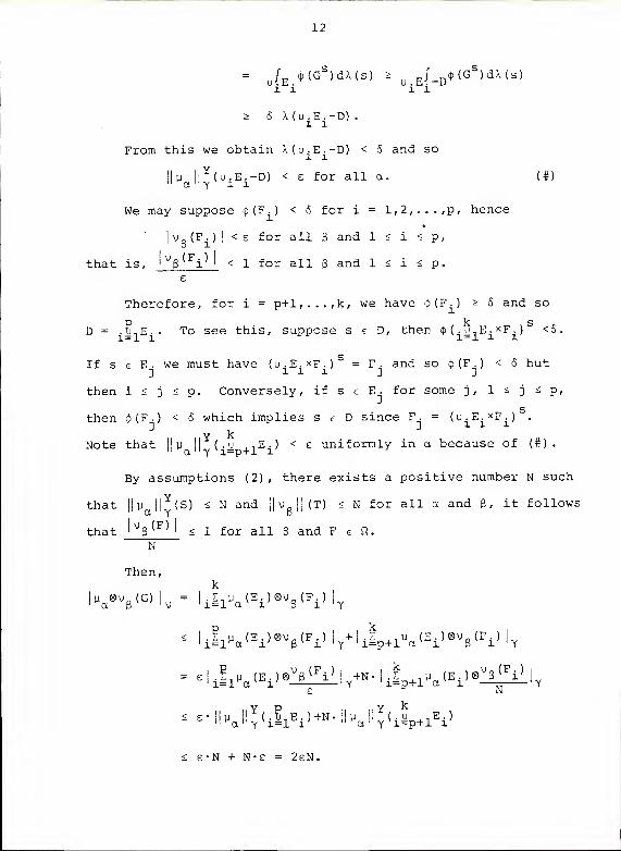
Proof . We must show to every e > 0, there exists a 6 >

such that whenever G e ft®A and Xx<j>(G) < 5 , we have

|y ®vR(G) | < c, for all a and 3.

To that end, let e > be given, there exists 6 > such that

X(E) < 6 implies ||y ||

Y(E) < e uniformly in a, and

(J)(F) < 6

implies |v D (F)| < e uniformly in 3.

k 2Suppose G = .ji-E.xF. € ft®A and Xx^ (G) < 5 where (E

i) £ ft

is disjoint and (F.) £ A.

Recall that for s e S, the s-section of G is

GS = {teT: (s,t)eG}.

k sWrite D = {s£

i^ 1Ei:<^(G )<6}.

We then have

62

> Xx<j>(G) = / <j>(Gs)dX(s)

12

=u /E

_<j)(GS)dA(s) > uE /_D

4>(GS)dA(s)

11 11

> 6 A(u.E.-D)11

From this we obtain X(u.E.-D) < <5 and so

11 u ||

Y(u.E.-D) < e for all a. (#)

11 a " y l l

We may suppose <j) (F .) < 6 for i = l,2,...,p, hence

|Vg (F. ) |

< e for all B and 1 < i < p,

that is, l

vg(F

i)

j

< 1 for all 6 and 1 < i < p.

Therefore, for i = p+l,...,k, we have <J>(F.) * 6 and so

p k sD =

. u,E.. To see this, suppose s e D, then $ (.u. E- X F. ) <6.

If s e E . we must have (u.E.xF.) = F. and so tj)(F.) < 6 but

then 1 < j < p. Conversely, if s e E . for some j, 1 < j < p,

sthen <$>(F.) < & which implies s e D since F. = (u.E.xF.) .

Y ^Note that II u || (.u ,,E.) < e uniformly in a because of (#).

'• a " y i=p+l i

By assumptions (2) , there exists a positive number N such

that|| y || (S) < N and ||v

g ||(T) < N for all a and 8, it follows

that l

V3(F)

j

< 1 for all 6 and F e ft.

N

Then,

,l ii 1 Ua

(Ei)®v

6(F

i )l

Y+l iip+1Pa

(Ei)0v

6(F

i)

|

y

- ^^(E^Z^I/N.lj^lE.,^^E N

, e-||ya N^( iS 1

Ei

)+N.||y

a |^( iup+1

E:L

)

< e-N + N-e = 2eN.

13

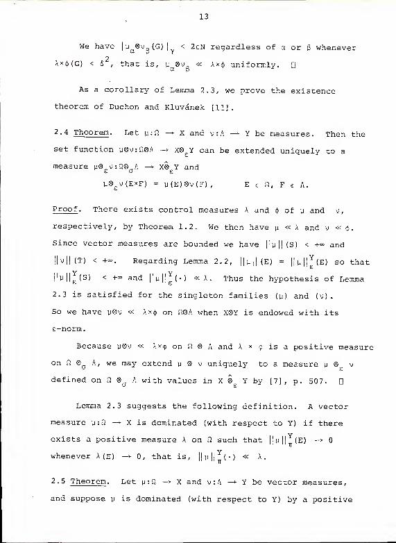
We have |ya®Vg(G)| < 2eN regardless of a or 3 whenever

2Ax<j,(G) < fi ' that is, y ®v_ « Axcp uniformly. Q

As a corollary of Lemma 2.3, we prove the existence

theorem of Duchon and Kluvanek [11]

.

2.4 Theorem . Let y : ft—* X and v:A — Y be measures. Then the

set function y®v:ft®A —> x®£Y can be extended uniquely to a

measure y® v:Q® A —* x® Y and

y®£V(ExF) = y(E)®v(F), E e ft, F e A.

Proof. There exists control measures A and of y and v,

respectively, by Theorem 1.2. We then have y « A and v « <{>.

Since vector measures are bounded we have ||y|| (S) < +« and

||v||(T) < +-. Regarding Lemma 2.2, ||y||(E) =||y||

Y(E) so that

i V V||y||

£(S) < +=° and ||y|| (•) «A. Thus the hypothesis of Lemma

2.3 is satisfied for the singleton families (y) and (v)

.

So we have y®v « Ax^ on fi®A when X®Y is endowed with its

£-norm.

Because y@v « Ax^ on n ® A and A x $ is a positive measure

on 0. ®a

A, we may extend y ® v uniquely to a measure y ® v

defined on Q ®q

A with values in X 8 Y by [7], p. 507. Q

Lemma 2.3 suggests the following definition. A vector

measure y:Q —> X is dominated (with respect to Y) if there

exists a positive measure A on Q such that ||y|| (E) -*

whenever A (E) —> , that is, ||y|| (•) « A.

2.5 Theorem . Let y : ft —> X and v:A —> Y be vector measures,

and suppose y is dominated (with respect to Y) by a positive

14

measure A. Then there exists a unique measure y@^v:fl®aA —

>

X® Y which extends y ® v; consequently, y® v (E*F) = u(E)®v(F)TT TT

for E e fl and F e A.

Proof. Choose a control measure <j> of v. Then v « <j> and

||y||Y

(-) « A. According to Lemma 2.3, y®v « \x<\> on fi ® A

provided |[y|| (S) < +°°. If this is shown, the theorem is

proven because the extension is guaranteed by [7], p. 507.

To show Null (S) < +°°, there exists 5 > such thatII M

|f

A(E) < 6 implies ||y||Y<E) < 1. By Saks lemma ([12], IV. 9. 7),

there exists E,,E2,...,E e tt disjoint such that S = u

iEi

Yand each E. is either an atom or X (E. ) < 6. Since ||u||

iT

(S) <

.£ ||y||Y(E.) and ||y|j^(E

i) < 1 for all those i for which

ME.) < <S, to show ||y||Y<S) < +°°, it suffices to prove that

if E is an atom, then ||y|| (E) < +co.

Let E e tt be an atom of A, that is, if G c E and G e Q

then X (G) =0 or A (G) = X(E). Because y is a-additive, it is

bounded, so we can find a number N such that| y (A)

|< N-A(E),

for all A e Q. Now for G c E, G e CI, either A (G) =0 (in

which case ||y||Y

(G) = 0, hence |y(G)( =0) or A (G) = A (E) ;

in either case, we have |y(G)| < NA (G)

.

Now

||u||Y

(E) = sup {| iE1y(G

i)®y i l

7T:yi

eY,|yi

|

< l,(Gi

) e n(E)}

< sup {iZ1|y(G

i ) |: (G

i)en(E)}

< N.J, A(G.)1=1 l

= N-A (E) < +°°,

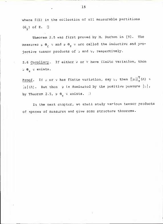
15

where 11(E) is the collection of all measurable partitions

(G. ) of E.1

Theorem 2.5 was first proved by M. Duchon in [9]. The

measures y ® v and y ® v are called the inductive and pro-

jective tensor products of y and v, respectively.

2.6 Corollary. If either y or v have finite variation, then

y ® v exists.IT

YProof . If y or v has finite variation, say y, then ||y|| u

(A) <

|y|(A). But then y is dominated by the positive peasure |y|,

by Theorem 2.5, y &^ v exists.

In the next chapter, we shall study various tensor products

of spaces of measures and give some structure theorems.

CHAPTER IITENSOR PRODUCTS OF SPACES OF MEASURES

1. Algebraic Tensor Products of Spaces of Measures .

M. Duchon seemed to have developed the theory of product

measures primarily for the study of Borel and Bairs measures

on locally compact Hausdorff spaces [8] and for the study of

convolutions of Borel measures defined on a compact Hausdorff

topological semigroup with values in a Banach algebra. Here,

however, we develope the study of tensor products of abstract

spaces of measures.

Throughout this chapter, (S,ft) and (T,A) will denote

fixed but arbitrary measurable spaces; X and Y are Banach

spaces.

The space ca(S,fi;X), or simply ca(fi;X), is the space

of all measures y : Q —* X. ca(Q;X) is a Banach space when

equipped with the semivariation norm ||•

||(S) . When X = $

,

we write ca(fi) instead of ca(fi;$). In this case, the semi-

variation norm is identical with the total variation norm

I- I(S).

When various subspaces of ca(ft;X) are under consideration,

descriptive letters are placed in juxtaposition with "ca," for

example: cabv(ft;X) is the subspace of ca(ft;X) consisting of

all those measures with finite total variation, Ccabv(Q;X)

is the subspace of all measures of finite total variation

and with relatively norm compact range. Any subspace of

16

17

ca(-Q;X) consisting of measures with finite total variation

will have as its norm, the total variation norm |

• |(S)

rather than the semivariation norm. Since||

•|| (S) &

| |

(S) ,

the total vairation norm defines on this subspace a topology

which is, ingeneral, strictly finer than the topology induced

by the semivariation norm.

Recall that from the universal mapping property of tensor

products, any bilinear map from the Cartesian product of two

Banach spaces into a third Banach space induces a unique

linear map from the algebraic tensor product of the first two

spaces into the third (see the remarks following Theorem

1.2.1). The following theorem establishes the basic algebraic

structure in which we shall be working throughout this chapter.

1.1 Theorem . (a) The bilinear map<f>

:(y,v) -* y®£v induces

an algebraic isomorphism which embeds ca(Q;X) ca(A;Y) into

ca(SxT,ft0 A;X® Y)

.

(b) The bilinear map <j> :(u,v) —* M® u vinduces an algebraic

isomorphism which embeds cabv(fi;S) ca(A;Y) into ca(S><T,

ft0 A;X0 Y)

.

a it

Proof. Since y0 v always exists whenever y and v are measures,

the map $ is defined on ca(ft;X) x ca(A;Y) and takes its

values in ca(M Q,-,X® Y);y® v exists whenever y has finite

total variation, so that <j> is defined on cabv(J2;X) x ca(A;Y)

and has its range in ca (J18 A;X8 Y) . It is not difficult to

see that <j> and<J>

are bilinear.

In order to prove that the unique linear maps induced

by<J>

and<f>

are isomorphisms, it suffices, according to

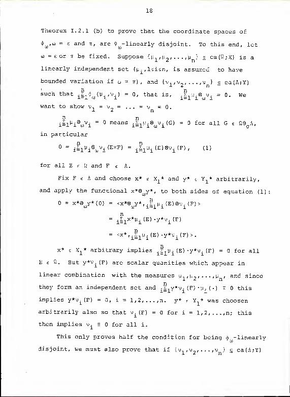
18

Theorem 1.2.1 (b) to prove that the coordinate spaces of

uitD = £ and tt , are $ -linearly disjoint. To this end, let

w = £ or 7T be fixed. Suppose {y , y2,...,y } £ ca(^;X) is a

linearly independent set (y.,l<i<n, is assumed to have

bounded variation if to = tt) , and {v,,v„,...,v } c ca(A;Y)12 n -n n

such that .Z 4 (y ,v ) = 0, that is, .I,y.® v. = 0. We1-1 0) 1 1 1=1 1 (j i

want to show v. = v„ = . . . = v =0.12 n

.Z y.0 v. = means .£,y.® v. (G> = for all G e ft® A,-L— X i tt) 1 1—1 1 U) 1 O

in particular

= i^iVi^^) =i£1 M i

(E)®vi(F) , (1)

for all E c \l and F e A.

Fix F e A and choose x* e X * and y* e Y * arbitrarily,

and apply the functional x*®wy*, to both sides of equation (1)

= x*® y* (0) = <x*® y*, . Z.y . (E)®v. (F)

>

coJ

or i=l l l

n=

i£ 1x*y

i(E) •y*v

±(F)

= <x*,iZ1yi(E) •y*v

±(F)>.

x* e X±* arbitrary implies

i| 1 P i(E) -y*v . (F) = for all

E e Si. But y*^i(F) are scalar quanities which appear in

linear combination with the measures \i^ ,\i~> , . • ,u , and since12 n

they form an independent set and .£-,y*v. (F)-y. (•) = this

implies y*v±(F) = 0, i = 1, 2, . . . ,n. y* e Y* was choosen

arbitrarily also so that V.(F) = for i = 1,2, ...,n; this

then implies v. = for all i.

This only proves half the condition for being c£> -linearly

disjoint, we must also prove that if {v,,v?,...,v } c ca(A;Y)

19

forms a linearly independent set and d-^/V^' • • • 'V^) - ca(fi;X)

such that . E,p.ev. = 0, then u = y = ... = u = 0. The1= 1 1 lii 1 ± £ II

proof of this is analogous to the above proof.

Thus the linear maps induced by <$> and ^ are isomorphisms

which proves (a) and (b) . Q

1.2 Corollary . cabv(Q;X) ® cabv(A;Y) c cabv (S^AjXQ^Y)

algebraically.

Proof. In view of Theorem 1.1, we have

cabv(fi;X) @ cabv(A;Y) c cabv(Q;X) 9 ca(A;Y)

c ca(ft® A;X® Y) .

It suffices therefore to prove that all measures in the

space on the left have finite variation. Let \i e cabv(fi;X)

. . ^n n „ n .

and v e cabv(A;Y) and take disjoint sets Gn

= j^^^i iin

ft®A, n = 1,2, ... ,p. Then

Jl^V (Gn>U * nil 5ilv(= 1

n)*v(Fin)|

ir

= nIlik

f1 l^^in )|-|v(F

i

n)|

^nlliflMO-MO- JlitlulxlvKE^F^)

= |y|x|v|(J LGn).

It follows that for any G e ft®A we have|

uQ^v|

(G) <

|u |

x.|v

|

(G) , hence for all G c ^10QA.

Thus |u® v|(Sxt) < |u|-<;|v| (S*T) < +°°, so that cabv(ft;X) ®

cabv(A;Y) consists of measures with finite variation and

therefore lies in cabv(fi®aA; XQ^Y) .

20

1.3 Remark . Duchon [9] has shown that |y® v[(G) =jy|x|v|(G)

for all G e fi© A whenever both y and v have finite variation. D

Topological embeddings of (a) in Theorem 1.1 will be

considered later in this chapter; first, however, we prove

the following theorem.

1.4 Theorem . (a) The bilinear map ty : (y,x) —> xy induces

an isometric algebraic isomorphism on ca(fi)® X into ca(ft;X).

(b) The bilinear map ty :(y,x) -* xy induces an isometric

algebraic isomorphism on ca(ft)® X into cabv(Q;X).

Thus ca(Q)® X c ca(fi-X) and ca(Q)® X c cabv(ft;X)e -

tt-

isometrically

.

Proof . The proof of that ca(fi)® X c cabv(ft;X) isometrically

will be postponed until Theorem 2.3 infra , where we shall

characterize this space; we state (b) now only for completeness.

It is clear that ca(Q)®X c ca(ft;X) by considering the

bilinear map (y,x) — xy , where xy e ca(ft;X) is defined by

(xy) (E) = x-y(E). Consequently, ca(f2)®X consists of all X-valued

n"step-measures" on 0, of the form . E,x.u.(«) for x. £ x andc i=l 11 i

y i€ ca(„Q) .

nThe step measure .Lx.ii. has finite total variation sincer i=l l i

y. has finite variation for each i = l,2,...,n. We can therefore

consider ca(S7)®X as an algebraic subspace of cabv(Q;X). Part

(a) claims that when we consider ca(^)®X as a subspace of

ca(^;X), the e-norm is exactly the norm induced on ca(^)®X

by ca(fi;X), namely, the semivariation norm. Part (b) claims

that the TT-norm is the total variation norm. Here we prove

the isometry of part (a)

.

21

nTo that end, let .Z.x.y. e ca(n)®X, From the general

theory, the s-norm can be defined as the norm of £.x,u-

when it is considered as a linear map from X* into ca(ft)

defined by <E.x.u,x*> = £ .x* (x. )M • • Thusj 1 l

K x XXXIZ.x.y. I

= fuP

.|£.x*(x.)y.

I(S)

=xf?g Jx*(£i

xipi

)|(s)f

(1)

= ll^x.uJKs) (2)

In going from (1) to (2) , we have invoked the Dinculeanu

result, Proposition I. 1.1. Thus the e-norm is equal to the

semivariation norm. Q

We now prove two technical lemmas followed by a theorem

which gives insight into the algebraic structure of vector

measures defined on product c-algebras and taking their values

in a Banach space X, that is, measures of the form \:ttQ A -* X.

This situation is, of course, a bit more general than measures

X of the form u® v , oj = e or ir , which take their values in

the tensor product of two Banach spaces.

1,5 Lemma. Let A,,A_,...,A be n linearly independent scalar1 2 n J ^

measures defined on fi. Then there exists sets E, ,E ,...,E12 n

in f2 such that the determinant of the n x n matrix (A. (E.))„ v „li

n A n

is non-zero. We write

$(A1,A-,. ..,A ;E, ,E-,...,E) = det(A (E.)) nxn * 0.

l 2. nlz n i 3 n*n

Proof . The proof is by induction on n.

Case n=2 . Suppose X ,A„ form a linearly independent set of

scalar measures on Q such that $(A, , A_;E, ,E„) = for all

22

choices of E, ,E2

e n « This means that

X1(B

1).X

2(E

2) - X

l(E2)X

2(El ) =

for all E ir E 2e SI. Fix E

2e fl and let E

1vary over Q. \

1

and X2

independent implies X2(E

2) = and A

1(E

2) = 0. Since

E 9was arbitrary we have X = X

2= 0, a contradiction.

Case n = k+1 . Suppose the lemma is true whenever n < k, and

that {X ,X , . . . ,A ,,X } is a linearly independent set of k + 1

scalar measures such that for all choices of E,,E2 , . . - E

k+1e ft

*<V X2 VW E1' E 2 Ek'W = °" (1)

Writing the determinent in (1) in terms of its first row

expansion:

ill(-l)i+1

Xi(E

1).$(X

1X.,..,,X k+1 ;E

2,E

3 V Ek-H

)= °' (2)

where X. means that X. is deleted from the list of entries.

Since the measures (X.}.^j" are linearly independent and

(2) is valid as E, varies over ft, we obtain

•<*1 V"" Xk+l

;E 2' E 3Ek'W =

° (3)

for any i and any choice of (E.)!£i eft. (3) is a contradictionJ j ^

of our induction hypothesis since we are back to the case

n = k.

By Theorem 1.1, the spaces cabv(ft;X) ca(A) and ca(ft) ®

cabv(A;X) lie algebraically in ca(ft8QA;X) and, in fact, lie

in cabv(ft8 A;X) ; consequently, we may consider the set-theoretic

intersection of these two subspaces:

I(ft,A;X) = cabv(ft;X)®ca(A) nca(ft)®cabv(A;X)

23

1.6 Lemma . If 9 e I(fl,A;X), then there exists an integer

n > 1 and vectors x,,x2,...,x , scalar measures V^/J^' * * * ,yn

€

nca(fl) and v i/ v2"*" v

ne ca(A) such that 8 =

i£ 1xi (y i

xvi

)

•

Proof. Without loss of generality, we may assume 8*0.P _

8 e cabv(ft;X)®ca(A) implies 8 =j_i 1

Vi®v

i

for y~. e cabv(ft;X) and v. e ca(J2). 8 e ca(fl) ®cabv (A; X)

implies 8 = .£ y.®\T. for u . e ca(fi) and \T e cabv(A;X).

We assume henceforth that p < n, and that each family

{y~}, {v.}, {y-}, {v~. } is a linearly independent family of

measures.

By Lemma 1.5, there exists sets F,,F2,...,F e A such

that $(v1,v

2, . . . ,v ;F,,F

2, .. .,F J

* 0. Write as simply $ * .

With this observation, we use Cramer's rule to solve

the system

v1(F

1)y~(-)+v

2(F

1)y~(-) + ...+v

p(F

1)y~ (•) = .1^ (F

]_) y . ( •

)

v1(F

2)y-(.)+v

2(F

2)y-(.) + ...+v

p(F

2)y~(-) = ^v" (F

2 ) y . (•

)

v1(Fp)y-

1(-) +v

2(Fp)y-

2(Fp)y-(.) + ...+v

p(Fp)y-(-) = .^v" (F

p) y .

(• ) .

Define for i = l,2,...,p and j = l,2,...,n the vector

x j = ^ • '- Vi-1

(Fa (i-D ) V

'iiF

o (i)} V i+1

{Fo (i+D } ' '

'

'

i ae sp

J-j

where S is the symmetric group on p-letters; obviously,

X"? e X for all i and j .

l— n i

Thus by Cramer's rule y ±(') =

-iiixi^-j(")

for x = 1,2/ ""P'

Substituting this into 8 = . £,vT®v. we get

24

Jl jIlX>j XVi)?

the lemma is proved upon re-indexing this representation. D

1.7 Theorem . I(n,A;X) = X®ca (fl) ®ca (A)

.

Proof. From Lemma 1.6 we have I(ft,A;X) £ x®ca (fi) ®ca (A)

since any member of I(Q,A;X) can be represented in the form

S.x.(y.xv.) where x. e X, u. e ca(fi) and v. e ca(A), which1111 i i i

clearly puts it in X®ca (ft)®ca (A)

.

Conversely, if 9 e X®ca(ft) ®ca (A) , then we can write

8 as 9 = E.x.m. where x. e X and m. e ca(fi)®ca(A). Let iill i 1

be fixed, we can write m. in the form m^ = £jM-j x v. where

y1

e ca(ft) and v1

e ca(A). Now we have that

x. (y1xv

1) = (x.y

1)® v

1e cabv(fi;X) ® ca(A), but

x.(u1xv

1) = y

1®(x.v1

) e ca(fl) ® cabv(A;X). Thus x. (y^xv.) eID J 3 x 3 ! 3 J

I(fl,A;X) and therefore x.nu = I.x^uNv^) e I(fl,A;X), and in

turn 8 = E.x.m. e I(J2,A;X). D

2. The Radon-Nikodym Property

We now introduce a notion which has not appeared in

the literature — that of the Radon-Nikodym property of a

measure.

A vector valued measure r:fi —> X which has finite total

variation is said to have the Radon-Nikodym property, or

simply the R-N property, if whenever X:Q. —> R. is a positive

measure such that x « X, then there exists a Bochner integrable

function f:S —*• X such that

25

t(E) = / £f dX

for all E e R. We say that f is the Radon-Nikodym derivative

of x with respect to X and write f = -tt- or dp= f dX

.

Recall that a Banach space X has the Radon-Nikodym

property if for every measurable space (S,fl) and any vector

measure x:ft —+ X of finite variation, x can be written as

an indefinite Bochner integral with respect to any positive

measure 1 on 2 for which x « A. Thus, the Banach space X

has the Radon-Nikodym property if and only if every vector

measure that takes its values in X has the Radon-Nikodym

property. The R-N property of a Banach space is a global

property whereas the R-N property of a measure is a local

property.

The R-N property of a measure is important in classifying

certain tensor products of spaces of measures. In preparation

for this, we establish an important lemma.

2.1 Lemma . Suppose x:ft —> X is a vector measure of bounded

variation such that x « X « v, where X and v are two positive

measures on ft. If x has a Radon-Nikodym derivative with respect

to v, then it has a derivative with respect to X.

Proof . By the Lebesgue Decomposition Theorem, write v = u+i

where y « X and i l X. Since i l X, there exists E e 0,

such that i(E ) = but X (S-E ) = 0. From u« X, there exists

h e L*(S,ft,X) such that u (E) = J £h dX

.

Thus

x(E) = /_f dv = /_f dU + / f di = / fh dX+ / f di

26

Assert that /_f di = for all E e J2.

Case I . E c E . Since i (E ) = 0, we must have i (E) =0

and so / f di =

Case II. E c s-E . Since A (S-E ) = 0, we have A (E) =0o o

and so /„fh dA = 0; furthermore, t «A and A(E) =0 implies' E

T(E) = 0.

Thus

= t(E) =/E

fh dA+/E

f di = 0+/£f di

or / f di = 0.

Cases I and II are sufficient to conclude / f di =

since E = (EnE ) u En (S-E ) and the integral /f di is additive.

Thus x(E) = Lfh dA, that is fh = ^ and the lemma isE uA

proved. D

2.2 Theorem . Let (t.) c cabv(ft;X) such thatk£1 hk

|(S) < +=°.

If x has the R-N property for each k e w, then so does the

00

measure t = ,Lt, .

Proof . We remark first that the infinite series E^ t^ does

define the measure because the series l^ t. (E) converges

absolutely for each E 6 2:

kJ1|Tk(E)

I

< jJjJtJ (E) <k| 1

|Tk|(S) < +» by hypothesis.

To show x has the R-N property, begin by supposing t << A

,

where A is a positive measure on ft.

Note that ,?, |x, |(E) converges and consequently defines

a a-additive measure on Q such that x^ «kI 1 l

Tk l

for each

n e a).

27

Write v = X+ El

T v l'then v is a positive measure on

Q such that X « v; consequently, T « X « v. We intend to

show t has a Radon-Nkodym derivative with respect to v,

and then use Lemma 2.1 to prove the theorem.

Indeed, for each n e u> we have also that x « v. xn n

has by assumption the R-N property; hence x (E) = / f dv

for some f e B (S,fi,v), where B (S,ft,v) is the space ofn x x

Bochner integrable X-valued functions.

Write |fn l 1

= /s|fjdv and note |tJ(S) = |f

n | r 1^^is the norm of f in B (S,Q,v)

.

n x

co - oo . ,

Since E, f , = E, T (S) < +°° and Bv (S,f2,v) is an=l ' n ' 1 n=l n X

Banach space, ?,f converges in norm to a function f er n=l n 3

CO

Bv (S,n,v), that is, f = E-f .

X n=l n

But then

t(E) =nSlTn

(S) = JJ^ dv = /E nIlfndv = /E

f dv.

That is, f = -r^. By Lemma 2.1 then, -r^- exists, which means,dv qa

since A was arbitrary, x has the R-N property. Q

We now prove a theorem which identifies the space ca(£3)® X.

This is a generalization of a theorem of Gil de Lamadrid [13] ,

where he identifies C*(H)®7TX, C* (K) is the dual of the Banach

space of all continuous functions on a compact Hausdorff

space H. C* (H) is of course the space of all regular Radon

measures on H. Our setting is based on an abstract measurable

space (S,fi) . Lamadrid' s identification was that CMH)®^ was

the class of all regular X-valued Radon measures of bounded

variation which can be represented as an absolutely series

28

of "step measures." Theorem 2.2 implies that such a represen-

tation does have the R-N property. Our approach is quite

different than his and the result was independently obtained.

2.3 Theorem . Let (S,ft) be a measurable space and X a Banach

space. Then ca(ft)® X is isometrically embedded in Ccabv(ft;X),

the space of all X-valued measures with bounded variation and

relatively norm compact range.

Furthermore, ca(fi)® X is the Banach space of all X-valued

measures on ft with the R-N property. Symbolically,

ca(ft)® X = RNca(ft;X)

.

TT

Proof . By Theorem 1.4, ca(ft)®X c cabv(ft;X). It is clearn

that any measure 8 = . L. x.A. e ca(Q)®X has relative norms 1=1 j l

compact range since each A. does. To show the initial assertion,

if suffices to prove that on ca(fi)@X, the ir-topology is identical

to the bounded variation norm. Indeed, if the n-norm on

ca(£2)®X is the variation norm then since Ccabv(Q;X) is a

Banach space, the completion ca(Q)§ X of ca(Q)®X is just the

closure of ca(ft)®X in Ccabv(ft; X) , hence ca(K)® X c Ccabv(fi;X).

nTake 6 =

. £,x.u. where x. e X and \i . e ca(fl) . Then1=1 11 l l

|0|(S) =| i| 1

xiy i

[(S) < .|1|x

i|-|y| (S).

If we take the infimum on the right hand sice over all represen-

tations of 9 in the form Z.x.u. we obtain |8|(S) < 19 I .

i iKi in' i i

-u

n nSuppose again 9 = . £ x.u. e ca(Q)8X, and put X = .Z.|y.|,

then p . « X for each i. Write f . = x which exists by the1

dA

classical Radon-Nikodym theorem. f. e L (a) and

29

f =ii 1

xifi

£ BX(A). Note that f = — , that |y i

|(S) = If^i

where | f.

| is the norm off. in L ( A ) , andj

[(S )

= | f|

^

,

where |fL is the norm of f in BX(X) .

Define 3 £ BX (A) and M £ ca(Q)®X as follows

k _ _ i k - ,

B = { .^ 1xi g i

:xieX,g

i£L (A), and f =

jJLixi9i

X ~a .e.

}

k _ k _M = { .£,x.v. :x.€X,v

ieca(n) and 9 =

i |:1xivi>-

There exists an injection ij;:B —> M defined by

k k k —di(.Z,x.g.) =

. E,x. /, ,g dA; furthermore if • I-.x.g. and

k. £,x.v. are in correspondence, then1=1 l l

Jil*~iH9ili- Ji |x"i'

ivi|(s) '

We conclude that

infj.lx-l-lgj, .inf^lx-l-lvjhS) (#)

for we have argued that for each number from the left side,

there is a number from the right side which is at least as

small.

It is well known that B (A) = X&^L1(X) isometrically

(see Treves [18]). Since f e B (A) we have that | f

|

1= |f|

ffr

but If^ = igf ilil^il-lgili so thatl

9l

< s) =l

f li= |f U'

kOn the other hand,

|6

| w= inf

j_I 1 1

x^^|

•|vi |

(S) .

Thus from (#), |8|(S) =|f

| ^ 2: 16^. We already have

|8|(S) < |9| so that |6|(S) = 16^, which proves the first

assertion.

We now prove ca(Q,)®^X = RNca^-X).

30

If x e RNca(ft;X), then x necessarily has finite total

variation; put X = |t|. Then x « X and since x has the

R-N property, there exists f £ BX(X) such that x(E) =/

£f dX

for all E e ft.

Since f is Bochner integrable, we may write f in the

form f(s) = Lx L (S) X-a.e., where x e X and E e ft

n=l n^E n n

(the family (E ) is not in general pairwise disjoint) , and

possessing the property that !il xn l

A ( En )< +°°- This is a

well-known result which can be derived from Theorem III. 5.

5

infra , or see Brooks [3]

.

Define x :ft -* X for each n e to by x (E) = x X (EnE ) .

n n n ii

x is easily seen to have the R-N property and t e ca(ft)®X,n n

also JJtJCS) =nSL

|xn|-X(S

n ) < +-. (1)

So we have

x(E) =J E

t dX = / E n!1XnCEn

dX - J^EoE^,

or x(E) = ?,t (E) for E e ft. (2)n=l n

nAs remarked above x

ne XQ^ca (ft) , hence j^^ e XQ^catft).

n oo . .

Note that (1) implies the sequence tkSiT

]c-rn=i

1S Cauchy in

X® ca(ft). From the first half of the proof, the ^r-norm isIT

equal to the variation norm, so for n < m positive integers

m m mLet, =

, z x, (s) < i xj (s) — oI k^n k ' 7T ' k=n k ' k=n ' k '

as n and m approach infinity because of (1) . Regarding (2) ,

E„x, must converqe in variation to x since it convergesk=l k

to x setwise. Therefore x e XQ^catft) since it is the sum of

a sequence (x ) in X® ca(ft). Thus we have RNca(ft;X) c XQ^catft)

31

Conversely, if t e X0 ca(Q), then from the general theory

of projective products (see Treves [18] , Cp. 45) , there exists

CO| || .

x e X and X e ca(ft) such that E. x • X (S) < +°° and suchn n n— i n n

that t (E) = ?,x A (E) , where the series will converge absolutelyn=l n n

in X. Write t = x A ; t clearly has the R-N property forn n n n

each n e oj, also t = ?„T and ?. I t I (S) < +<*>, We concluden=l n n=l ' n

'

from Theorem 2.2 that t has the R-N property and so x e RNca(ft;X).

Therefore X® ca(fi) c RNca(ft;X), hence we have equality. D

2.4 Corollary . A measure y:fi —> X with bounded variation has

the R-N property if and only if y is expressible as an indefinte

Bochner integral with respect to some measure \:ti —> R .

Proof . If f has the R-N property, then y is expressible as

an indefinite Bochner integral with respect to any measure

with which y is absolutely continuous.

Conversely, if y (E) = / f dA for some positive measure

A, then there exists a sequence of simple functions (f )

converging to f A-a.e. such that | f -f j . =/ s

|fn-f|d\ -+ 0.

Write y (E) = / e f dA ; consequently, y^ e ca(fi)® X. Wen o n n n

will show that y e ca(ft)® X so that by Theorem 2.3, y will

have the R-N property. Because ca(f2)®7TX is isometrically

embedded in cabv(fi; x), it suffices to show that the sequence

y e ca(ft)® X converges in variation to y. This is indeed

the case because |y -y|(S) = |fn"f|iand Ji^ooH f

n~ f

II 1 = 0. D

2.5 Corollary . A Banach space X is a Radon-Nikodym space if

and only if ca(S,ft)® X = cabv(S,ft;X) for every measurable space

(S,fl)

.

32

Proof . One always has ca(S,H)§ X c cabv(S,^;X) to begin

with. If X is a Radon-Nikodym space, then that means any

X-valued measure on ft has the R-N property, that is, we have

containment in the other direction, hence equality.

Conversely, if ca(S,fl)® X = bvca(S,Q;X) for every measur-

able space, then, regarding Theorem 2.3, this means every

X-valued measure of bounded variation has the R-N property

regardless of the measurable space (S,ft). This is the definition

of X being a Radon-Nikodym space. Q

2.6 Remark . In particular ca(S,Q)@ X = bvca(S,^;X) if X is

a reflexive Banach space of if X is a separable dual space. Q

We have shown by Theorem 2.3 that ca(ft)Q X lies isometrically

isomorphically in Cbvca (fi;X) . The question is raised whether

this isomorphism is onto. The answer is no in general as

demonstrated by the following example.

2.7 Example . This is an example of a vector valued measure

with bounded bariation and relative norm compact range which

does not have the R-N property. This is an example due to

Yosida [19]

.

Let S = [0,1], fl = 8 the a-field of Baire sets of [0,1]

and A: 8 — R the Lebesgue measure. Denote by m [1/3,2/3]

the Banach space of real-valued functions E, - C(9) defined on

[1/3,2/3] and normed by ||c|| = sup|£(9)|.8

Define an m [1/3 , 2/3] -valued function x(s) = £(9;s) on

[0,1] by :

| if o < s < 6;

x(s) (9) = £(9;s) = I ,

|3 if 9 .< s * 1.

33

Yosida has shown that x(s) satisfies the Lipschitz

condition: |x(s)-x( s ')| < 3 1 s- s '| for all s,s' e [0,1].

Define a set function on the class of intervals of [0,1]

by x(I) = x(s)-x(s') where s is the right end point of I and

s 1 is the left end point. The set function x has its values

in m[l/3,2/3], and extends to the class of Baire sets on

[0,1] as a set function with values in m[l/3,2/3]. Because

of the Lipschitz condition, |x(B)| < 3A (B) for B e 8 , ito

follows x is a-additive, A-continuous, and of finite total

variation. Yosida has shown in [19] , that x cannot be

expressed as a Bochner integral with respect to Lebesgue

measure A even though x « X. We shall show that x has

relatively norm compact range.

According to Dunford-Schwartz [12], IV. 5. 6, a bounded

set K in m [1/3, 2/3] is relatively compact if and only if for

every z > 0, there exists a finite collection {E, ,E-,...,E }12' n

of disjoints sets with union [1/3,2/3] and points 8 e E,

such that sup |f (8)-f (6, ) |< e, for all f e K and k = 1,2,3,. ...n.

0eEkk

It shall be shown that {x(l):lel}, where I is the algebra

of unions of disjoint intervals of [0,1], is relatively norm

compact in m [1/3, 2/3].

Because x is a-additive, its range is bounded.

Let e > be given. Choose n so large that 1/n < e.

FOr k= °' 1 ' 2 9n- X'^fine E

k=

(| +^, § + |±i). E_

k

has length 1/27 n. Write 6 as the midpoint of E, .

Let < k < 9n-l and I e I be fixed. We claim for any

9 e Ek

that |x(I) (9)-x(I) (9 k ) |< e.

34

Suppose to begin with that 9 e E, and 8, < 6 . We may

m i+iwrite x(I) in the form x(I)(6) =

iI 1(~l) ~*(s

±) (Q) , where

S]_

> s2

> s3

> > s

Let q be the largest integer such that s > 9 and p4 K

be the greatest integer such that s > 9. Since 8, < 8,P K

we have p < q.

Thus,

x(I)(8) =4 £ 1 (-l)-

TX5(8#s.) = .S^-l) 1* 1 ^ J

ny

i=li+1 r ,

i=l i^ +i-S+i'

-1 '

i+1 s.

and

.(DCe^-J^-D^Vi*^.-!) 1*1!!.

So that

x(I) (9) - x(I) (9 k ) |

=

V 1

.? l( -l)i+1 B

i-1

-si-

1

X L 9-1 9,-1k

+ .?4. 1

(-Di+1 S

i -Si_1

+ •?+1 (-D

i+1 Si "

Si

1=P+1 X 97^T1=q+1 — 87

Simplifying, we get9 -9

x(I)(9) - x(I)(9k )! < .^(-D^^s.-l)

(__ ljrv „

;L)

l.,(-Di+1

sk

- 9

i=p+l l 8 (8.-1)i

+ l4+1 -'i+1 '->

(6k-l)

m i+1ak

(- 1)

lsiW,i=q+l

Write |x(I) (8) - x(I) (9k ) |

< Q1

+ Q2

+ Q3

+ Q4

(1)Q-l

= 8k-e

(9k-l) (8-1)

ig1(-l)

i+1(s

i-l)|s 2

(8 k-l) (8-1)

< 18 9. -9 < -=-r- since1 k ' 54n

,9, e E, which has half width

of l/54n.

So Q, < ~.1 3n

3 5

(2)

36

Throughout this section V:& —* X is a measure, and

\:tt —y R+

is a control measure for y. We shall denote by

II the collection of all measurable partitions of S; that

is, it e II if and only if tt = {F ,F2,...,F } where F. e Q are

npairwise disjoint, X (F

.) > and S = . u -F . . Partially order

II as follows: for tt , tt ' e II, write tt > tt ' if and only if every

member of tt lies in some member of tt' .

For each tt e II, define y :ti —> X by

^ (E) =fItt X7fT

xf(e)

'for E e n '

and where A„(E) = A (EnF) . Since A is a control measure wer

have that y « y and in fact A„ « u; also, observe y (F) = y (F)TT F TT

for each F e tt .

It is clear that for each tt e n, y^ £ ca(fi)8 X and with

the partial ordering of H, (y ) is a net (or generalized sequence)tt

of measures in ca(ft)® X (See Dunford and Schwartz [12], Section

1.7). We shall show that if y has relatively norm compact

range, then lim y = y is semivariation.

3.1 Lemma . If the Banach space X is the scalar field, then

lim |yff-u| (S) =

Proof. Because y « A and y is scalar valued, there exists

a A-integrable function f such that y (E) = / f dA for each

E e n, by the Radon-Nikodym Theorem.

For tt s IT, define

V s> - fItt aTfT/f

f d^ V s)'

s e S;

consequently, we have

ME) = L f dPTT

J E TT

37

From [12] (IV. 8. 18), lim f = f is L1(X) . Because the

TT n

L (A) -norm of a function is the total variation of its indefi-

nite integral, we have limlu-y |(S) =0. DTT IT'

We use this lemma to prove the same result for the general

case of X being an arbitrary Banach space and y a measure with

relatively norm compact range. We remark that Theorem 3.2

was proven by Lewis [16] ; here we present a more direct proof

of the theorem.

3.2 Theorem . If p:(l -> X is a vector measure with relatively

norm compact range, then lim i! y-y II (S) = 0, and consequently,TT TT

y e ca(n)®£X.

Proof. Let A, II and (y ) be as above, and defineTT

ca(ft,A) = {<j>eca(fi) :<j>« A}.

Define on ca(£2,A), for each tt e II , the linear operator

U^ by U d> = <}> , where <j> e ca(ft,A) . By Lemma 3.1, lim U<J)

= <p

in ca(fi,A); consequently, by the Phillips' Lemma [12, IV. 5. 4],

lim U d> = <jj uniformly on compact subsets of ca(n,A) .

For each x* e X,*, we have x*y e ca(fi,A) so that

l^mlU^ (x + y)-x*y|(S) = lim|x*y -x*y

|(S) = 0.

Since sup |x*y -x*y|(S) = |jy -yll(S), in order to showx*eX, * it

'

tt

lim|| y -y|| (S) = 0, it suffices to show, therefore, that

lim|x*y -x*y| (S) = uniformly for x* e X *, that is,

lim U (x*y) = x*y uniformly for x* e X,*. From the aboveTT TF

J 1

discussion, we need only show that V = {x*y:x*eX *} is a

compact subset of ca(^,A).

38

To this end, let (x *y) £ V; we shall show that there is

a subsequence which converges in variation. Since V is weakly

sequentially compact by [12, IV. 10 . 4] , there exists xQ* e X,*

and a subsequence (x* ) of (x *) such that x* y — xQ*y weakly

in ca(fi,A), that is lim x* y (E) = x *y (E) for each E e fi.

i ni

u

Since y has relatively norm compact range, the set R = {y(E):EeP„}

is relatively compact in X; but x* — x * pointwise on R implies,

by the Banach-Steinhaus theorem, x* —> x * uniformly on Rn.

Jy

Thus, lim sup |x* y (E) -x n *y (E) |= 0. But then

ii EcP ' ^ MV'

= lim sup |x* y(E)-x *y(E)| > \ lim|

x* y-x *y|(S)i E£i2 "i

u ! i

(see the remarks following Proposition I. 1.1).

It follows then that x* y —* x *y in variation, and thatn.l

r is compact. Thus limlly -y||(S) = 0.IT <*

Finally, y e ca(Q)® X since it is the limit in norm of

a net (y ) of elements from ca(fi)® X. GTT £

3.3 Theorem . ca(ft)® X = Cca(Q;X) isometrically , where Cca(^;X)

is the Banach space of X-valued measures with relatively norm

compact range.

Proof. It is clear that any of the step measures which comprise

the space ca(fl)0X have relatively norm compact range because

they are linear combinations of elements of X with bounded

scalar measures; consequently, each step measure is bounded

with range in a finite dimensional subspace of X, hence has

relatively norm compact range.

By Theorem 1.3, ca(ft)® X is isometrically embedded in

ca(Q;X) and consequently in Cca(fi;X). The closure of ca(fi)®£X

39

in Cca(ft;X) is ca(ft)0 X and ca(ft)§ X £ Cca(ft;X). By Theorem

3.2, we have reverse inclusion. Q

3.4 Corollary . If (S,ft) and (T,A) are measurable spaces with

X and Y Banach spaces, then

Cca(SxT,ft® A;X® Y) = Cca (S, ft; X)

®

£Cca (T, A; Y)

.

Proof . This follows from Theorem 3.3 and the associativity

of the inductive tensor product of four Banach spaces. Q

3.5 Corollary . ca(SxT,ft® A) = ca (S , ft) ®£ca (T , A) .

Proof . Any scalar measure has a bounded range, hence a

relatively norm compact range.

4. The Space ca (ft ; X) ®^ca ( A; Y)

In this section (S,ft) and (T,A) are measurable spaces

with X and Y Banach spaces. We shall prove that the e-norm

on ca (ft;X)®ca (A; Y) is the semivariation norm, and that

ca(ft;X)0 ca(A;Y) can be isometrically embedded in a certain

space of separately continuous bilinear maps.

Recall that X*®Y* is a vector subspace of (X©£Y)* since

each x* e X* and y* e Y* defines a linear functional x*®£y* e

(X® Y) * such that <x*® v*,x®y> = x*(x)-y*(y) and |x*9 y* |

=

|x*|*|y*|. Observing the definition of the e-norm, we see that

the set

r = {x*® y* : x*eX1*, y*eY

1*}

is a norming family for X® Y. Also, for each y e ca(ft;X),

v e ca(A;Y), x* e X* and y* e Y*, the linear functional x*®£y*

acting on the vector measure y® v yields scalar measure defined

40

by:

<x*® y*, y® v> (G) = x*y xy*v(G),

where G e ft® A

.

Thus, x*® y* can be thought of as a linear map from

ca(ft;X) ® ca(A;Y) into ca(ft®aA); furthermore, x*®

£y* is

continuous when the former space has on it the e-norm and

the latter space is supplied with the total variation norm.

We prove this in the next lemma.

4.1 Lemma . Let x* e X* and y* £ Y*. x* ® y* when considered

as a linear map from ca(ft;X) ®£

ca(A;Y) into ca(ft©aA) defined

by <x*® y*, y® v> = x*y x y*v is a continuous linear map.

Moreover, |x*® y*| = |x*|*|y*|.

Proof . The maps <x*,y> = x*y and <y*,v> - y*v are defined

from ca(ft;X) (resp. ca(A;Y)) into ca(ft) (resp. ca(A)), are

both clearly linear and they are both continuous since by

Proposition I. 1.1,

|x*y|(S) < |x*|-||y|| (S) and |y*v|(T) < |y* |•

|| v ||(T) .

From the general theory of tensor products, the map

x*® y* is continuous from ca(ft;X) ®_ ca(A;Y) into ca(fi)® ca(A)

(see Treves [18], Theorem 43.6), and |x*®£y*| = |x*|-|y*|.

The map x*® y* can be extended to ca (Q; X)

®

£ca (A; Y) with

values in ca(fi)® ca (A) . By Corollary 3.5, ca(ft®aA) =

ca(ft)® ca(A) . Q

From this lemma, we observe the next proposition which

shall be used in this chapter and in Chapter IV.

41

n4.2 Proposition . Let. . Z y . ® v. e ca(fi;X) ® ca(A;Y). Then

the semivariation of this measure is given by

|| i| 1 y i®evi ||

(SxT) = sup| i| 1

x*uixy*v

i |

(SxT) ,

where the supremum is taken over x* e X,* and y* e Y i*-

Proof. The collection T = {x*® y*:x*eX * and y*eY *} ise 1 1

a norming family for X® Y ,- therefore by Proposition 1,1.1,

n

iS^^v.IKsxt) =

(x*^5 )er l<x*®£y*,

i4 1 Mi®evi>l(Sx T )

The proposition follows then from this equality and

Lemma 4.1. Q

If we now endow ca(Q;X) ® ca(A;Y) with the semivariation

norm it is easy to see from the above proposition that this

is a cross norm:

II P® v|I(SxT) = sup|x*uxy*v

|

(SxT) = sup|x*y|

(S) • |y*v|

(T)

= Hull (S) • ||v|| (T) ,

where all supremums are taken over X * x Y *.

Also from Lemma 4.1, we have ||0|[(SxT) < |8| for any

e ca(i'2;X)®£ca(A;Y) ; indeed, for x* e X,* any y* e Y * the

function x* ® y* is continuous and |x*® y* |= |x*|*|y*| = 1

so that |x*® y*9

|

(Sxt) s |6| . Now taking the supremum over

X * x y^^* we get by Proposition 4.2, ||9||(Sxt) < |e| . We

shall see that in fact, equality reigns.

4.3 Theorem . For any 9 e ca(ft;X)® ca(A;Y), we have ||9||(Sxt)

| 9 | , that is,

ca(n,-X)® ca(A;Y) c ca(Q® A;X® Y) isometrically

.

42

Proof . Let y*e ca(fi;X)* and v* e ca(A;Y)* and consider

y*®v* e ca(Q;X)* ® ca(A;Y)*. The norm of y* 8 v* associated

with the semivariation norm is defined by

|y*®v*| = sup|i| 1y*(M i

) •v*(vi

) |, (1)

where the supremum is taken over all elements p =. £ u.® v.1=1 1 £ 1

such that ||p||(SxT) < 1. We claim that this norm is a crossnorm:

|y*®v*|

= |y*|•|v*|

.

It is clear that |y*|*|v*| < |y*®v*| by considering the

supremum in (1) as being over a smaller class, namely, over

all p = y®£v such that y e ca(Q;X), v e ca(A;Y) and ||p||(SxT) < 1,

Now let p = Zi y

i® v. be arbitrary with ||p|j(SxT) < 1.

Since y* is a linear functional on ca(Q;X) and Z.v*(v.)y. e

ca(ft;X) we have

|ZiP*(u

i) •v*(v

i) |

< |y*| • ||Ziv* (v

i )u i j| (S) . (2)

Choose (E.) c n, a finite collection of pairwise disjoint

sets and scalars (a.) c $ with|a .

|< 1 such that

|U*| •||2iv*(v

i)y

i || (S) <§ + |u*|-|SjajZiv*(v

i )y i(E

j}

|

£+ [y*|-|v*|- ||Z.a.Z,y, (Ejv.ll (T) .2 + |y*l-|v*|-l|z

joj

i:

i u i(E

j)v

i

Again choosing sets (F, ) c A pairwise disjoint and scalars

(3k ) £ $ with |8k |< 1 such that

|y*|.|v*|.||Zja.Z

iy i(E

j)v

i ||(T)

< | + |y*|.|v*|.|ZkBk

EjajZiy i

(Ej)®v.(F

k )

|

Combining these inequalities with (2) we get

|Ziy*(y

i) •v*(v

± ) |

< e+|y*| •|v*|-|^j^k

ct

jSk

Zi y i

®£vi(E

jxF

k )i

(3)

4 3

Now since the family {E..x.F } . is pairwise disjointj k 3 , k

and covers S x T, and |a.g|

< 1 for all j and k, we see thatJ k

the quantity on the right hand side of (3) is one of the numbers

overwhich the supremum is taken in the definition of the

semivariation of the measure £.y.® v..11 e l

Thus,

|ZiM*(y i

) •v*(vi

) |

< £+|y*| • |v*| • ||Sini»evi ||

(Sxt) .

But now since p = I.y.® v. was arbitrary with ||p|| (SxT) < 1,

taking the supremum over all such p, we get by definition

|y*®v* |< E+| u*

|

•| v* | .

Since e > was arbitrary, we get |y*®v*| < |u*|*|v*|

and the assertion that |y*®v*| = |y*|*|v*| is proved.

Finally in order to prove |8| = ||8|| (Sxt) for any

8 e ca(fi;X)® ca(A;Y), if suffices to prove this for 8 of

n ,11111the form . E.y.Qv.. We have shown that y*®v* = y* • v* ,

this means

|y*®v*(8)| < |y*®v*| • ||8 ||(SxT) =

|

y*|

•|v*

|

•|| 8

||(SxT) .

So that

|9|e

= sup|Ziy*(y

i) •v*(v

i )

|

= sup |<y*®v£2.y.® v.>|

< sup|y*| -|v*| ||8|] (Sx T )

=||8

||(SxT ) ,

where the supremum is taken over |y*| =1 and |v*| = 1.

Thus, |8| <|| 8

)](Sxt). Since we have already observed

the reverse inequality, the theorem is proved, Q

44

4.4' Corollary . ca(Q;X)® Y c ca(n;X®£Y) isometrically

.

Proof . Let T = {0} and A = {T,cf>}, the power set of T, then

ca(T,A;Y) = Y isometrically. Apply Theorem 4.3. Q

Let X,Y, and Z be Banach spaces. Then b (X,Y; Z) will denote

the vector space of all separately continuous bilinear maps

from X X Y into Z. Separately continuous bilinear maps need

not be bounded; however, they are bounded whenever each factor

of the product space on which they are defined is a dual space.

For this reason, the space B(X*,Y*;Z) can be normed by

|b| = sup | b (x*,y*) | where the supremum is taken over X *xY *.

This topology on B(X*,Y*,Z) is the topology of uniform

convergence on equicontinuous (simply bounded) subsets of

X* x Y* of the form A * B. B(X*,Y*;Z) equipped with this

norm topology is denoted by B (X*,Y*;Z). It is not difficult

to see that B (X*,Y*;Z) is a Banach space.

Analogous to the usual embedding of ca(ft;X)® ca(A;Y)

into B (ca(fi;X) *,ca(2;Y) *;$) , from which the definition of

the e- topology was derived to begin with, we have the following

theorem.

4.5 Theorem . There exists an isometric isomorphism from

ca(ft;X)® ca(A;Y) into B (X* ,Y* ; ca (Q® A) )

.

Proof . Define @ :ca(U;X) * ca(A;Y) -*- B (X*, Y* ;ca (ft®aA) ) by

@(u,v) (x*,y*) = x*y x y*v. g is a bilinear map; using once

again the universal mapping property of tensor products,

there exists a unique linear map

®:ca(ft;X) ® ca(A;Y) -> B (X* , Y* ; ca (fi®aA) ) such that

®(y® v) (x*,y*) = x*y x y*v.

45

To prove that 8 is a one-to-one and an isometry, it

suffices to show it is an isometry.

ni

Let 6 = . Z,y.® v., and prove ®(8) = 6 .

|®(6)j = sup|Q (6) (x*,y*)|

= sup| i|1

x*y xy* v ](SxT)

=|| || (SxT) where the supremums are taken over X,* x y, :

By Theorem 4.3, |9| = ||9||(Sxt).

Thus I 8(9) |= |9| . D

There are a few advantages as well as disadvantages to

embedding ca(Q;X)® ca(A;Y) in B£(X* , Y*; ca (ft®

aA) ) rather than

B (ca (Q;X) *,ca (A;Y) *;$) . Because we know very little of the

structure of the duals of ca(fi;X) and ca(A;Y), it may be

advantageous to use the embedding B.(X* ,Y*;ca (£2® A) ) , the

structure of the Banach spaces X* and Y* may be well-known or

more easily worked with. The range space of the bilinear

maps of B (X* , Y*;ca (ft® A) ) is more complicated than the scalar

bilinear maps of the other embedding, though quite a lot is

known of the structure of ca(ft® A). At any rate, both

embeddings induce the e-norm on ca(ft;X) ® ca(A;Y).

CHAPTER IIIPETTIS AND LEBESGUE TYPE SPACES

AND VECTOR INTEGRATION

1. Measure Theory

Throughout this chapter, (S,ft) is a measureable space,

X and Y are Banach spaces, and y:ft —*- Y is a vector measure.

A set A c S is y-null if there exists a set E e ft such

that A c E and ||y||(E) = 0. The phrase "y-almost everywhere,"

or y-a.e., refers to u-null sets.

An X-valued ft-simple function is a function of the form

f(s) =. E,x. C_ (s) , where x. e X, (E

.) e ft is pairwise disjoint,

l—l it. l il

and £_ (s) is the characteristic function of E. . The setsEi

X

E. are called the characteristic sets of f. The vector spacel

of all such simple functions will be denoted by S (ft) , and

when X = $, by S(ft). A function f:S -*- X is y-measurable if

there exists a sequence of simple functions from sx ( fi ) converging

to f pointwise y-a.e. The same function is weakly y-measurable

if for each x* e X*, the scalar function x*f is y-measurable.

Obviously, any y-measurable function is weakly y-measurable;

the two concepts coincide if X is separable, by a theorem

due to Pettis [17]. A scalar function f:ft -+• $ is ^-measurable

_ \provided f (B) e ft for every Borel set B. Any ft-measurable

function is y-measurable, and any y-measurable function is

equal y-a.e. to a Sl-measurable function.

A sequence (f ) of y-measurable functions converges in

y-measure to a function f means

46

lim||li||([|f -f|> € ]) =n il

for each e > 0. In this case, f is y -measurable and there

exists a subsequence (f ) which converges pointwise to f

y-a.e., this is the theorem of F. Riesz. The Riesz theorem

and the Egorov theorem are valid for vector measures because

we can choose a control measure X for y. The measures y and

A have the same null sets, and therefore the same measurable

functions; convergence in y-measurable is equivalent to

convergence in A-measure . Since these two theorems are

valid for X, they are valid for y as well. Consequently,

any sequence of functions converging y-a.e. also converges

in y-measure. The phrases "in y-measure" and "y-a.e." are

virtually interchangeable.

2 . Normed Spaces of y-measurable Functions .

If f is weakly y-measurable, we can consider a number

of scalar integrals associated with f in order to define a

variety of seminomas on the space of X-valued weakly y-measurabls

functions.

Define the two seminorms N and N* on the space of weakly

y-measurable X-valued functions as follows:

(1) N(f) = supjs|f|d|y*y|;

1

(2) N*(f) -(x*su

?)eXi *xYiJs|x*f|d|y*y|.

We remark that N and N* are indeed seminorms because each

is the supremum of seminorms. Since (x*f | s ]f J

pointwise

for x* e X*, we have immediately that < N*(f) < N(f) < + =°.

48

The N-seminorm, which is a Lebesque-Bochner type, was

introduced by Brooks and Dinculeanu [5]; this seminorra will

sometimes be referred to as the strong seminoma. The N*-

seminorm, which is a Pettis type seminorm, will be called the

weak seminorm. These seminorms, of course, depend on many

parameters such as the measure u, and the Banach spaces X

and Y; it will be clear from the context which parameters

are being considered.

If f is X-valued, then |f | is scalar valued, and we shall

write N(f) = N*(

| f |) . Note that it is always the case that

N*(f) = sup N(|x*f|).x*ex,*

We list some properties of these seminorms

2.1 Proposition . (1) N and N* are subadditive and homogeneous;

(2) N*(f) = N(f) for f scalar valued;

(3) N*(f) = sup N*(f? ,), N(f) = sup N(f? .);

(4) N(sup f ) = sup N(f ) whenever (f ) is increasingn n n n n

and positive;

(5) N(E f ) £ £ N(f ) for every sequence of positive

functions (f )

;

n

(6) N(lim inf f ) < lim inf N(f );x' n n n n

(7) N(f) < +» implies f is finite y-a.e. for f R*-valued.

Proof. Numbers (1), (2), and (3) are clear from the definitions.

(4): sup N(fn ) = sup sud /s

|fn |d|y*y|

=y^*

SnP /sfn d|Y * P|

V^* ^SSHP f

nd

I y* U

l

= N(SHP fn } '

49

(5): N(E f ) = N(sup If) = sup N( If)n n k n=l n k n=l n

< sup ZJ(f ) = Z N(f ) .

k n=l n' n n'

(6): From Fatou's lemma,

/slim

ninf|f

n|d|y*y| < lim

ninf

/

g|

f

R| d |y*y |

.

So for y* e Y*

/slim

ninf|f

n|d|y*u| < su^lim

ninf J s |

fj d |y*y|

= lim inf sup L |

f

n |d|y*u

|

y*eY. *J S l n

= lim inf N(f )

.

n n

Finally, (6) is obtained by taking the supremum of the

left-hand inequality over Y *.

(7): If f is R*-valued, and N(f) < +», then for each y* e Y *,

f is finite |y*y|-a.e., from the classical theory. By Theorem

1.1.2, u-null sets are determined by only a countable family

of {|y*y|}, that is, there exists (y *) c Y * such that a subset

A c S is y-null if and only if A is |y *y|-null for each

new. As a result, f is finite u-a.e.

The set F (S,^,y;Y) of functions f:S —* X which areA

y-measurable and satisfy N(f) < +ro is a vector space with

seminorm N. When no confusion will arise, we write F (y)

for Fv (S,Q,y;Y) . The set Wv (S ,

Q

f y ; Y) , or simply Wv (y), isXX X

the set of all functions f which are X-valued and y-measurable

that satisfy N*(f) < +°°. W (y) is also a vector space with

seminorn N*. It is clear that F (y) c W (y) and the topologyx x

induced on F (y) by the seminorm N* is weaker than the N-norm

topology of F (y) since N*(f) < N(f).

50

Brooks and Dinculeanu [5] have shown, and it follows

from (5) in Proposition 2.1, that the system (F (y) ,N) is

a Banach space if functions equal y-a.e. are identified.

(W (y) ,N*) need not be a Banach space however, since it mayX

not be complete, even if functions equal y-a.e. are identified

We can make W (u) into a complete metric space by con-A

sidering the metric:

d(f,g) = N*(f-g) + inf {a+||y|| ( [jf-g| >a] ) }, f,g e W

x(y).

Recall that the second term in the definition is itself

a metric equivalent to convergence in y-measure (see Dunford

and Schwartz [12], p. 102^.

2.2 Proposition . The semimetric space (W (y),d) is complete.

Proof. Suppose (f ) £ Wv (u) is d-Cauchy, then (f ) is Cauchyn x n

in y-measure; consequently, there exists a function f from S

into X which is u-measurable and to which (f ) converges in

y-measure, that is, lim|| y || ( [ |

f -f|>e] ) = 0, for each e > 0.

n n

To show lim d(f ,f) = 0, it suffices to show lim N*(f -f) = 0.n n n n

Let x* e X,* be fixed. Since |x*f -x*f j<

I

fn-f

I

pointwise, we must have x*f —> x*f in y-measure too. Now

for each y* e Y±*, J s

| x*fn~x*fm

| d |y*y |

< N*(fn-fm), so (x*f

n >

is Cauchy in L. (y*y) , the classical Lebesgue space. But

x*f —* x*f in y-measure implies x*f —* x*f in y*y-measure,n n

so therefore x*f —> x*f in L, (y*y).

Let e > be given, choose K e oj such that whenever

m,n > K, N* (f -f ) < e.

ButJ

|x*f -x*f |d|y*y| < N* (fn-fffl) <£ ' for every

(x*,y*) e X1*xY

1* and m,n > K.

51

Because x*f —* x*f in L, (y*y) for each (x*,y*) e X^x 1^*

we have lim L|x*f -x*f |d|y*y| = L | x*f -x*f |d jy*y |

.

m o n iu onm

Therefore, for n > K,

/ |x*f -x*f|d|y*y| = lim / |x*f -x*f |d|y*y |s e.on m "

Taking the supremum over X **Y*, we get N* (f -f ) < e for all

n > K. D

This semimetric topology of W (u) is the topology whereA

a sequence (f ) c W (y) converges to a function f in V?x (y)

if and only if N* (f -f) —> and f —> f in y-measure. It

is possible, though we shall not do so here, to consider a

slightly more general space, the space of weakly y-measurabl

e

functions with finite N*-seminorm.

We next prove that N* is a norm on W (y) , if we agreeA

to identify two functions which disagree only on a y-null set.

2.3 Proposition . If f e W (y) and f = g y-a.e. for some X-valued

function g on S , then g e W (u) and N*(f-g) = 0, in particular,A

N*(f) = N*(g) .

Conversely, if N*(f) = 0, then f = y-a.e.

Proof . It is clear that g is y-measurable since it is equal

y-a.e. to a y-measurable function.

Now for each x* e X* and y* e Y * , x*f = x*g y-a.e.,

and therefore |y*y|-a.e. since |y*y| < ||y|| by Proposition

I. 1.1. This being the case, from the Lebesgue theory of

integration we have / |x*f-x*g |d |y*y |= 0. N*(f-g) = is

obtained by taking the supremum over X,*xY1*.

Conversely, N*(f) = implies sup__ /c |

x*f |d |y*yI

= 0,x*eX* °

for each y* e Y *. This supremum is the Pettis norm of f

52

with respect to the measure |y*y|; it follows then from

Pettis [17] that f = |y*y|-a.e. By Theorem 1.2.1, we have

f = y-a.e. D

Thus the space (W (y),d) is complete metric space; inX

fact, it is a Frechet space. To see this, it suffices to

show that lim d(af,0) = 0, where a e $ and f e Wv (y). This

fact was proven in Dunford and Schwartz [12], p. 329.

Notice that S„(Q) is a vector subspace of both F (u)A A

and W (y) . We shall denote by Bx (y) , the closure of Sx

(ft)

in F v (y) and remark that B (u) is a Banach space with normX A

N. Pv (u) will denote the closure of Sv (ft) in the metricX A

topology of W (y) ; P v (y) is a Frechet space.X A

As a result we have

(1) f e Bv (y) if there exists a sequence (f ) £ S (ft)X n a

converging y-a.e. to f such that lim N(f -f) = 0.n n

(2) f e P (y) if lim N*(f -f) = for some sequenceX n n

(f ) c S v (ft) converging y-a.e. to f.n x

For a simple function g we have N*(g) < N(g), therefore,

Bv (u) £ P v (y). If X = *, we write B v (y) = B(y) and Py (y) = P(y)XX A A

2.4 Proposition . B(y) = P(y) and N(f) = N*(f) for all f eB(y).

Proof . By Proposition 2.1 (2), N(f) = N*(f) whenever f is

scalar valued and y-measurable . Thus N = N* on S (ft) so

B(y) = P(y) . D

2.5 Proposition . Any bounded, y-measurable, X-valued function

on S is in B (y)

.

53

Proof. Let g:S —> X be bounded and y-measurable and write

K = suplg(s) |. There exists a sequence (g ) c S (ft) convergings £ 5 n a

in y-measurable to g and uniformly bounded by 2K.

For given e > 0, there exists Mew such that n > M

implies ||v|| ( I |g-g | >e] ) <e. Write En

= [Jg-g |>e].

When n > M,

N(g -gn }=

yi^§1* / s

|g-gn id|y*p|

'Y*e?f /EJ

g-gJ di y *

yl

+y^§* / S-E

nl g

-gnl d l y*M

l

£ 3K.||U|| (En ) + E-Hvll (S-E

n )

< 3K£ + £• ||p|| (S) = e(3K+||y|| (S) ) .

Therefore, lim N(g-g ) = and g e B (y) . D

Because Bv (y) c W (y) , it follows that W (y) containsXX X

the bounded, y-measurable functions too.

2.6 Propos i tion . A function f e W (y) is in P (y) if and onlyx x

oo

if lim N* (f C. ) = for every sequence (A ) c Q with fhA„ = db

.

n A n n— i nn

Proof . HJ Suppose f e P (y) , then letting e > be arbitrary,

choose a simple function g such that N*(f-g) < x.

Now if (A ) c fl and n.A = dp, and K = supjg(s)|

, thenn n— x n s e S

there exits Mew such that n > M implies ||y|| (A ) < ^ .

For n > M,

N*(fC ) < N*(f-g) + N*(g?A ) < | + K- ||u|| (An ) < e.

n n

(*-) Assume N* (f C, )—* whenever n n A = a.

v' ^A n=l n v

n

Put B = [If I <n] and A = S-B„; obviously „!!,& = *. fCr,n ' ' n n n— x n o

is bounded, so it is in Py(w) by Proposition 2.5. Since

lim N*(f-fc_, ) = lim N*(f?_ ) = by assumption, f e Pv (y). Dn B

n n An

X

54

2.7 Proposition . For f e W (y) , f £ P (y) if and only if

N*(fs(#)

) «y.

Proof . The condition N*(f?. .) «y means for any e > 0,

there exists 5 > such that if ||y|| (A) < 6, then N*(f£a ) < e.

(—^ Let £ > be given, choose a simple function g so that

2KN*(f-g) < §. Put K = sup|g(s)|, then for II y II (A) < -% we

have

N*(f?A ) < N*(f-g) + N*(gcA )

< | + K-N*(CA ) = | + K- !|u|| (A)

K!

+ K2~K

= £ '

Thus for|| y ||

(A) < ^ , we have N* (f X, ) < e.

(+-) Let n,A =tf> . Then |[y|| (A )

—> so by assumption

lim N*(fC, ) = 0. This implies by Proposition 2.6 thatn n

f e Px (y) . D

2.8 Remark . In Propositions 2.6 and 2.7, the properties

of N* that distinguish it from N where not used; consequently,

2.6 and 2.7 remain valid when W (y) , Pv (y) and N* are replacedA A

with F (y) , B (y) and N, respectively.AX3. Convergence Theorems .

We now consider convergence properties of the N*-norm

in order to obtain criteria for a function to be in px (y)

given that it is the pointwise limit of a sequence of functions

in PX(H)

•

3.1 Theorem. (Vitali Convergence Theorem) Let (f ) £ Pv (y)— - -—— il A

and f:S -> X. Suppose (1) f —> f in y-measure;

(2) N*(f L, x ) «y uniformly in n.\

v n ( •

)

Then f e Pv (y) and lim N*(f-f ) = 0.A H H

55

Conversely, if f —> f in P (y) , that is, in the d-metric,

then (1) and (2) hold.

Proof . We first show that (f ) is d-Cauchy. Since by

(1) , (f ) is Cauchy in y-measure, it suffices to show this

sequence is N*-Cauchy.

For s > given, there exists, by assumption (2) , a

5 > such that ||y||(A) < 5 implies N* (f c ) < J for all

new.

f —* f in y-measure implies the existence of M e oj

such that. ||y ||([|f

n-fm |

>jrfl ^H (s)

]) < 6' when n ' m - M -

Fix m,n > M and write B = U fn" fm l

>3

| |y

£

| |

(S)I •

N*(fn-fm ) <- N*(f

n-fm CB ) + N*(WS.B )

S N*(fn CB ) + N*(fm CB ) + N*(f

n-fm C s _B )

3 3 3-riuH (S)rJ U S-B ; ~

So (f ) is N*-Cauchy as well as in y-measure, thus

(f ) is d-Cauchy. Since Py (y) is complete and f —> f in

y-measure, we see that lim N*(f -f) = and f e P (u).n n x

Conversely, suppose d(f ,f) — 0; then f —* f in

y-measure and N*(f -f) —> 0.n

Let e > be given, there exists Mew such that n > M

implies N*(f z, ) < N*(f? ) + | for all A e n. This follows

from the inequality

N*(f £J - N*(f?J * N*(f -f) .

n^A A n

Since feP v (y), we have N*(f£, ,) «y. Thus there existsA ( •

)

a 6 > so that N*(f£ ) < -| whenever ||y|| (A) < 6. For n > M,

N*(f <;J < N*(fC») + |<-| + |-=£ whenever ||y|| (A) < 5.n A A z z z

56

Because f,,f2,...,f

M e px (u), it must be true that N* (f^c .

.) « y

,

for k = 1,2,...,M. There are only finitely many, so we may

find a single 5, > such that ||y||(A) < 6, implies N*(f ? ) < e,

1 < k < M. Finally, putting 5- = min {5,6 }, we see that

N*(f £,) < e for all new whenever ||y||(A) < S~. This is

condition (2) ; condition (1) follows from the assumption

that d(f ,f) -* 0. Dn

3.2 Theorem. (Lebesgue Dominated Convergence) Let (f ) c P (y) .— n a

Assume g e P(y) and f:S — X such that

(1) f —v f in y-measure;n

(2) |f|

< |g| pointwise y-a.e. for every new.

Then f e Px (y) and N*(fn~f)

—> 0.

Proof . Note that |x*f|

< |f|

< |g| pointwise y-a.e. for every

n e u and x* e X * . Let A e fl.

N *(Va> = xSS^ NU * fn^ " N(^A } '

g e P(y), and P(y) = B(y), so N(g£, .) «y

by Proposition 2.7. By the above inequality we then have

N*(f L. ,) «y uniformly in n e oj.n^ ( •

)

By the Vitali Theorem 3.1, f e ?x (u) and N* (f

n~f )

-*- 0. Q

3.3 Corollary . (Bounded Convergence) If |f|

< M pointwise

y-a.e., for every n, where M is some positive constant, then

f e Px (y) and N*(f

n~f) -+ 0.

Proof . Put g(s) = M for s e S. g is a constant function so

g e P(y) by Proposition 2.5. Apply Theorem 3.2. Q

57

3.4 Remark. No crucial role was played by the N*-norm;

consequently, the Vitali and Lebesgue Dominated Convergence

theorems are valid when N* and Pv (u) is replaced by N andA

B (u) , with only minor changes in the proof.

Brooks and Dinculeanu [5] have studied the space Bx(y)

in more detail and generality. Under suitable conditions,

the space B (u) is weakly sequentially complete, a workable

dual space has been identified, and sufficient conditions

have been given for subsets of Bx (y) to be weakly compact.

The space Py (M) is more difficult to work with because it

is not a Banach space but a Frechet space.

4 . Integration .

Let y:ft —* Y be countably additive and X a Banach space.

In this section we develop an integration theory for functions

in P„(y) and Bx(y) .

Suppose f(s) = .|, xi ? E

(s) where x^e X and (E^ c ft

forms a measurable partition of S, define for any E e ft,

Lf ® dy = .Z,x.® y (EnE. ) .1 E £ 1=1 l l

We note that the value of the integral of a simple function

lies in the space X Y.

4.1 Proposition . (1) The integral of a simple function is

well defined.

(2) The integral is linear, homogeneous,

and countably additive.

Proof . Suppose f =i|1

x^g and g = .J^ Xj ?A _

. Then

n m _f"9 " iil j=l

(Xi-

XjKE.A,

and

/Ef ®

£dy -

/£g ®

£dy = il-jX^ y(EnE

i)

- .J^x ®y(EnA.)D=l 3 J

n= . I. x.®(;.E,y (EnE. nA . ) )

- .1, x.® ( . Z, y (EnE . nA . ) )1=1 l 3 = 1 i j 3 = 1 3 i=l i 3

n m m n= .Z\ .Z n x .®y (EnE. nA. ) - .Z, . E , x .®y (EnE . nA

.

)

1=1 3=1 3 i 3 3=1 1=1 3 13n m .

= ,£, .Z, (x.-x.) ® y(EnE. nA ) = J_f-g ® dy .

1—1 j — 1 13 * j " *

This proves the linearity and uniqueness; indeed, if

f = g y-a.e. then whenever ||y|| (E nA.

) * 0, we have x. - x. = 0.1 3

1 -J

It is always true then that ||y[| (EnE^A. ) = or xi

- x". = 0;

therefore

,

, , n m _/ E

f ®£dy -

/ Ef ®

£dy =

i|=1 j^ 1

(xi-x

j) ®y(EnE

inA

j) = 0.

This proves the integral is well defined.

In order to show the countable additivity of the indefinite

integral of a simple function, it suffices to consider a simple

function of the form f(s) = x£E(s), for some x e X and E e fi

.

00

indeed, if (A ) c Q is disjoint and A = u,A , then sincen n=l n

00

y is a-additive, y(EnA) = E y (EnA ) converges unconditionally

in Y.

00

It is clear that J, x®y(EnA ) converges unconditionally

in X® Y andE

00 co

Z,x®y (EnA ) = x® E,y(EnA ) = x®y (EnA .

n=l M n n=l n

But this is equivalent to

Lf® dy = Z.L f® dy. DJ A e n=l J A e

n

4.2 Propositon . Let f e S (ft) . Then for every (x*,y*) e X**Y*,

(x*®£y*) JE

f®£dy = JE

x*fd(y*y).

59

Furthermore,

|J Ef®

edy|

£< N*(fCE ).

Proof . The first assertion follows immediately upon writing

the integral as a finite sum determined by the simple function

f. The cannonical image of X * x Y * in (X ® Y) * is norming

for X ® Y so that£

|/ Ef®

£dy|

£= sup

|(x*®

£y*)|

Ef®

£dy|

= sup |/ sx*(f?

E)d(y*u)

|

£ N*(f?A ) ,

where the supremum is over (x*,y*) e X * x Y *. D

4.3 Corollary. Let f e Sv (fl) and x (E) = / f® dy , for E e Q.

Then t : <T2— X ® Yisa vector measure and t« u.

e

Proof . The fact that t is a vector measure follows from

Proposition 4.1. Observing Proposition 4.2, |t(E)| < N*(fC£ ).

N*(fc, x) « U by Proposition 2.6, so t « y. D

5. The Weak and Strong Integrals .

Consider a function f e P (y). There exists a sequenceA

(f ) c S„(fi) which converges to f in y-measure and lim N*(f -f)=0.n — x n n

The sequence (f ) is said to determine f. Now, for each E e fl,^ n

the sequence {/^f ® dy} is Cauchy in the norm of X Y.n J E n £J £

Indeed, by Proposition 4.2,

|/_f ® dy - /^f ® dy I< N*(f -f )

.

IJ En£ ; Em£'£ n m

Define /_,f® dy = lim /_f ® dy , E e fl.E £ n E n £

This integral takes its values in X ® Y and is called the

weak integral of f over E with respect to y

.

The weak integral in unambigously defined for if (f )

and (g ) both determined f, then lim N* (f-f ) = and

60

lim N*(f-g ) = 0.n n

|Lf ® dy - /_g ® dul < N*(f -g )

< N*(f -f) + N*(f-g )

From this we see that

lim /_f ® dy = lim /_g ® dy

.

n J E n c n J En e

Let now f £ B (y) and (f ) £ S (ft) a determining sequencex n x

for f in B v (y), that is, lim N(f-f ) = 0.

Because

|/_f -8 dy - / f ® dul < N(f -f ) ,IJ Ene ; Eme'e n m'

we see that the sequence (/pf ® dy } is Cauchy in the norm

of X Y; hence, it tends to a limit in that space.

Define the strong integral of f by

/ f® dy = lim /_f dy , for E e fl.J E e n J EneSince B v (y) c P v (y) and the norm N < N*, it follows

X X

if f e B v (y), then any sequence in S (ft) that determines f

in B v (y) also determines f in P (y); consequently, a determiningX X

sequence for f in B (y) defines the same value in X® Y forX t.

both the weak and strong integrals. In this way we see that

the strong integral is well defined and can be unambiguously

denoted in the same way as the weak integral.

We next consider the countable additivity of these

integrals as well as a decomposition theorem for weakly

integrable functions.

5.1 Propositon . The indefinite integral of a weakly (resp.

strongly) integrable function is countably additive.

61

Proof . The countable additivity of the strong integral will

follow from the countable additivity of the weak. To that

end, let f e Px (u) and write T (E) = /E

f®£dy, where E e Q.

.

There exists a sequence (f ) of simple functions that determines

f in Px(y) •

If x (E) = jff ® du, then by definition lim t (E) = x (E)n J E n e

J n^ 00 n

for every E e Q..

By Proposition 4.1, each x is countably additive, and

by Corollary 4.3, x «y for each new; therefore, by the

vector form of the Nikodym theorem ([12], IV. 10. 6), x is

countably additive. Q

5.2 Proposition . If f e P (u) , then for each x* e X * and

y* e Y *, we have x*f e L (y*y), the classical Lebesgue space.

Furthermore, /px*f d(y*y) = (x*® y*) /„f® dy

.

Proof . The first assertion follows from the inequality

/ |x*f|d|y*y| < N*(f) < +°°. The left-side of this inequality

is the L1-norm of x*f in L

1(y*y), that is ||x*f||

1< +°°. The

second assertion follows by considering a determining sequence

for f, Proposition 4.2, and the continuity of x*® y*. D

5.3 Proposition . If f e px (y) '

thenI ^E

f®e

dvi' e

" N*(fC£).

If f e Bx (y), then |/E

f®£dy|

£< N(fC£ ).

Proof . For f e P (y)

,

--'- x

/ f® dyl = sup |(x*® y*)/ f® dyE e

= sup |/ sx*(f?

E) d(y*y)

|

62

< sup / |x*(f£_) |d|y*y

= N*(f?E

)

.

The second assertion follows because B (u) <= Pv (y) and

N*(f) < N(f) . D

5.4 Theorem. If h = .£,x.c_ e P,r (y), where x. eX and thei=l i s E. X l

l

family (E.)£ ft is pariwise disjoint, then for each E e ft

we have

. 00

Jh® dy = .2, x.®y(EnE.), and the series converges

unconditionally in X © Y.

Proof . Define t (E) = / h® dy

.

00

Since x is a-additive, Proposition 5.1, and S = -y.-,E. ,

00 00

we have x (E) = x(.u.EnE.) = . Z,x(EnE.) where the last series1=1 l i=l l

converges unconditionally in X 8 Y.

Now for each i, x{EnE.) = /_ _ h® dp, and for (x*,y*) e1 riDt • £

X * x Y *, we have

x*® y*x(EnE.) = f„ _ x*h d(y*u) = x* (x.

) -y*y (EnE .

)

zJ l ; EnE. * 1 J l

l

= x*® y* (x.®u (EnE. ) )

.

But this implies x(EnE.) = x-®y(EnE.) because {x*® y* |(x* ,y*) e

X * x Y *} is norming for X ® Y.

Thus /„h® dy = x (E) = .?,x(EnE.) =.|, x . ®y (EnE . ) converges

unconditionally in X 8 Y.

5.5 Theorem . (Decomposition Theorem) Suppose f e P (y)»

then f can be written in the form f = g + h y-a.e., where

(1) g is bounded (hence g e B (y));

(2) h = .?,x.£„ where x. e X and E. e tt are disjoint.v

' 1=1 i E, ii

63

Furthermore

,

(#)/ f® du = /^g® dy + . £. x. ®p (EnE. ) where the last series

converges unconditionally for each E e ft.

Proof . Since f is y-measurable , it has an almost separable

range, so that we assume from the beginning that the range

of f is separable.

Let a 10 be summable. Define, for each n, S(n,f(s))n

to be the sphere of radius a about f (s) . For each n, f (S) £

u S(n,f(s)). The range of f is separable metric space —

hence it is Lindelof; consequently, there exists a sequence

(s.n

) in S such that f(S) £ *u°S (n, f (s^) ) .

Pettis has proved in [17] that the function s—> | f (s) -f (s . )|

is u-measurable, hence A.n

=- |f-f(s.n)| ([0,a ) ) eft is y-measurable

Define E±

n= A

j_

n- gj Aj,

nand write f

R(s) = ^"f (s^Hj, (s).

Note that for each n, S = . u,E. and E. n E. = ({> for i * j.1=1 l l jT J

Obviously, for any n, and s e S , we must have s e E. for some

i; but this implies that ]f (s)-f (s. ) |< a and, therefore,

If (s) - f (s) I< a . This means f —> f uniformly on S.

1 n ' n n J

Write g(s) = I, (f ,,(s)-f (s) ) , then g is measurable,3 n= 1 n+ 1 n 3

and bounded since |g(s)|< I, If ,,(s)-f (s) I < 2 E,a .1

' n=l n+1 n n=l n

Finally, define E. = E. , x. = f(s. ) and h(s) = f,(s) =

• ^ftS. 1)^ 1(S) = ^,(3).

1 1

We clearly have f(s) = g(s) + h(s), for all s e S, because

f(s) = iiip.fn(s) = f

x(s) + iti< f

n+i<s>-V s)) - h < s >

+ g< s >-

64

g is bounded so that g e Py (y) (Proposition 2.5); consequently

h e P (y) , since h = f - g and f,g e Px (y).

(#) follows from Theorem 5.4. Q

The Decomposition theorem is similar to the one published

by Brooks in [3]

.

We now turn to a deeper study of the weak and strong

integrals by comparison with well known, more familiar integrals.

6. The Weak Integral and its Relationships to Other Integrals .

The purpose of this section is to explore the various

relationships between the weak integral, the general bilinear

integral of Bartle [1], and a Pettis-type integral which will

be introduced below.

Let us first consider the Bartle general bilinear integral.

Bartle considers y-measurable functions f : S —+ X and a measure

y:ft — Y with a bilinear map b from X * Y into a third space

Z. In our context, b:Xxy -+ X8 Y is the canonical bilinear

map defined by b(x,y) = x®y. Note that jb(x,y)| = |x|-|y|.

Bartle requires the "control" set function for the measure

p to be|| y |!

:Q —> R , the semivariation of y with respect to

X (and e), defined in Chapter I. From Lemma 1.2.2, we have

that ||y||Y

(A) = ||y||(A) for every A e Q. Consequently, Bartle ' s

control set function turns out to be the "usual" one. It is

important to note, that the measure then has the *-property

(see Bartle [1] )

.

In order for a function f from S into X to be integrable

in the sense of Bartle, there must exist a sequence (f ) cs (.1)n a

65

converging y-a.e. such that the sequence {/„f dy } is Cauchy

is the norm of X ®^ Y for each E e fi, where the integral of

a simple function is defined in the usual fashion. In this

case, one defines

(B)/Efdy=lim/

Efndu.

We say the sequence (f ) determines the Bartle integral of f.

We now consider the relationship between the weak integral,

defined for functions in P (y), and the Bartle integral.A.

6.1 Theorem . A function f:S —> X is Bartle integrable if and

only if f e P (y). Moreover,

(1) a sequence (f ) £ S y(^) determines the Bartle integral

of f if and only if lim N*(f -f) = 0;n n

(2) / f 8 dy = (B)/ f dy for every E e 12.

Proof . If f e P (y) , then there exist a determining sequence

(f ) c Sv (8) for f in Pv (u), that is, lim N*(f-f ) = 0. Fromn x a n n

our observations preceding the definition of the weak integral

in section 5, the sequence {/„f ® dy} is Cauchy in X 8 Y

for every E e Q. Since the Bartle and weak integrals of simple

functions obviously coincide, (f ) determines the Bartlen

integral of f , f is Bartle integrable, and

/ Ef ®

£dy = (B)/

£f dy.

Conversely, suppose f:S —> X is Bartle integrable, that

is, there exists a sequence (f ) c S (P.) converging to f

y-a.e. such that lim /_ f dy exists in X Y for everyn J E n £

E s Jl, the limit being (B) / f dy . We wish to show f e P (y) ,

to do so, it suffices to show that lim N*(f-f ) = 0, this willn n

also prove (1)

.

66

Write

x (E) = (B)Lf dy and x n (E) = (B) /_f dy , E £ ft.

Bv the definition of the Bartle intearal, lira x (E) = T n (E)• n n u

for each E e ft. The measures x are integrals of simple

functions so they are a-additive and xn« y for each n e uj;

consequently, by the vector form of the Vitali-Hahn-Saks theorem

(see [12,111.7.2]) , we have xn« y uniformly for new.

Because |x*0 y*x I< II x II for x* e X * and y* e Y *,

we have|x*® y*x

|

« y uniformly for n e oj, x* e X^* and

y* e Y*. Note that |

x*0£y*x

n |(E) = J£

| x*fR

| d |

y*y|for E e ft.

Taking the supremum over X,* x Y,*, we have N *( fn ?(.))

<<: y

uniformly in n e oj. But f -* f y-a.e., and N*(fn?,

») « y

uniformly implies by the Vitali Theorem 3.1, that f e Pjj(u)

and lim N* (f -f) = 0. The validity of (2) follows becausen n

(f ) determines the weak and Bartle integrals of f .

n

In [12] , Dunford and Schwartz developed a theory of

integration of scalar valued functions with respect to a

vector valued measure. This theory is that of Bartle' s for

X = 0, in this case we shall say a scalar function is Bartle-

Dunford-Schwartz integrable, or B-D-S integrable. We have

the following corollary to Theorem 6.1.

6.2 Corollary . A scalar valued, y-mearurable function f is

B-D-S integrable if and only if f e P(y).

6.3 Remark. By Proposition 2.4, P(y) = B(y); we shall denote

this space by D(y). From Corollary 6.2, D(y) is the Banach

space of all scalar functions which are B-D-S integrable with

respect to y.

67

7. A Pettis-type Integral .

In this section, we will introduce an integral which

is more general than the weak integral in the sense that

more functions are integrable. The definition of this integral

is reminiscent of B. J. Pettis' integral introduced in [17],

and it will be shown that for strongly measurable functions,

P v (y) is exactly the class of all functions integrable in

the new sense. Again, y:ft —> Y is a-additive.

A function f:S —> X is X® Y- integrable, or Pettis-integrable

,

on a set E e ft, if there exists an element 8_ e X® Y such that

for all x* e X* and y* e Y* we have x*®£y* (9

E) = /E

x*fd(y*y).

We shall denote the element 8 by (P)/ f dy . A function of

this type is X® Y-integrable if it is X® Y-integrable over every

set E e ft. Any X® Y-integrable function is weakly y-measurable

.

Because X* ® Y* is a subspace of (X®£Y) * which is norming

for x® Y, the Pettis integral as defined above is single

valued, linear, and finitely additive. Note that if Y is the

scalar field, then this integral is Pettis' "weak" integral.

7.1 Theorem . If f is X® Y-integrable, then the range of the

indefinite integral of f is bounded.

Proof. Put t (E) = (P)/^ f dy and consider the familyE

K = {x*® y*i:x*eX * and y*eY1*}.

We have K c ca(S,ft)

.

For E e ft, |x*®_y*i(E)| < |x* |

•|y*|

•

|

t (E)

|

£=

|

t (E) |.

This shows the set K to be pointwise bounded; by a result

of Nikodym ([12], IV. 9. 8), the set K is uniformly bounded.

68

that is, there exists a number M such that |x*® y*x(E) | < M

for all x* e X * and y* e Y *. Taking the supremum over

X * x Y * we get j x (E) j< M for all E e Q , that is, x is

bounded.

7.2 Corollary . If f is an X 8 Y-integrable, then N* (f ) < +°°.

Thus if f is y -measurable, f e W (u)

.

Proof. By Theorem 7.1, sup|

(P) / fdy/| < M,Eett " £

for some number M.

Consequently, for x* e X,* and y* e Y * we have

/s|x*f |d|y*u| < 4 sup|/

Ex*fd(y*y)

|

= 4 suplx*®r.y* (P)/,,f du|

Eefi e b

< 4 sup|(P)/

fif dy

|

< 4M < +oo.

If f is n-measurable and N*(f) < +°°, then by definition,

f e Wx(u) . D

We now prove the countable additivity of the indefinite

integral of a Pettis-integrable function. Pettis proved that

the weak integral of [17] was countably additive by showing

weak countable additivity implies countable additivily; in

our context, it is not clear that we have weak countable

additivity.

7.3 Remark . The dual of X ®£

Y is J(X,Y), the space of integral

forms on X x y. For any functional z e (X®£Y)*, there exists

closed and bounded subsets P c X* and Q c Y* and a positive

69

Radon measure v on the w*-compact set P x Q with total variation

< 1, such that for all 9 e X® Y

z(9) = /pxQ9(x*,y*) dv(x*,y*).

Here we consider 9 as a bounded bilinear map on X* x y* restricted

to P x Q ; the integral is the ordinary Lebesgue integral.

7.4 Theorem . Let f be X® Y-integrable. Then the indefinite

integral of f is countably additive.

Proof. Suppose (E.) c Q is a disjoint family and E =. u,E..

l - J 2 o 1=1 1

Write t (A) = (P)/,f dp for A e fl. We want to show . ?,t(E.)J A K 1=1 i'

converges unconditionally in X ® Y and converges to t (E )

.

Because of the Pettis lemma ( [12] IV. 10 . 1) , it suffices

to prove that t is weakly countably additive, that is,

<z,x(E )> = .Z,<z,t(E.)> for each z e (X® Y) * with |z] <1.i=l i e '

'

Let z be fixed.

Indeed, z is an integral form on X x Y, regarding Remark

7.3, there exists closed and bounded subsets P c x* and Q c Y*,

and a Radon measure v on P x q such that

z(9) = /pxQ9(x*,y*) dv(x*,y*), for 9 e X®£Y.

Define Ti(x*,y*) = / x*f d(y*y) for i = o,l,2,

i00

Note that T (x*,y*) = -I-.T. (x*,y*) for x* e P and y* e Q,

and that T. e C (P*Q) for i = 0,1,2,....

Write K = sup {|x*[-|y*| : x*eP and y*eQ} < +°° , and

since x is bounded by Theorem 7.1,

M = sup|T (A)

j< +°°.

AeH £

Finally, define F = .u.E., then for x* e P and y* e Q we have1 n i=l l 2

70

Li1Ti(x* f y*)| =

| i21/E_x*f d(y*u)

|

= |/ x*f d(y*y)

|

n

= |<X*8 V*, (P)/p f dU>n

< |x*|.|y*l'I (P)/F

f dy|n

< K-M < +«.

n oo

Thus the sequence {.Z,T.} , is pointwise dominated by^ i=l l n=l

K'M on P x Q. By the Lebesgue Dominated Convergence Theorem

/pxQT (x* ; y*)dv(x*,y*) = J^/p^i (x* ,y*) dv (x*,y*) .

But this says

<z,t(Eo)> = /pxQ <T(Eo ), (x*,y*)>dv(x*,y*)

= /PxQ <(P)/Ef dy, (x*,y*)>dv(x*,y*)

= /px0 /Ex*f d(y*y) dv(x*,y*)

o

=/px Q

To(x *' y *

) dv (x *'**)

=ili/pxQ

Ti(x*'^* ) dv(x*,y*)

= iL/pxn/E x * f d ^*^ dv(x*,y*)i

=il 1 /pxQ

<(P)/E

f dy, (x*,y*)>dv(x*,y*)

=i£1

<z,x (Ei

) >

.

That is, <z,t(E )> = .?, <z ,x (E .) > , and the theorem is

proved.

7.5 Theorem . If f is X® Y-integrable, then the indefinite

Pettis integral of f is absolutely continuous with respect

to y

.

71

Proof . Write t (A) = (P)/ f dy ; t is an X® Y-valued measure

on ft by Theorem 7.4; consider K c ca(S,ft) defined by

K = {x*® y*x:x*eX * and y*eY *}.e 1 1

It is clear that K « y, that is, x*® y*T « y for each

x*® y*x e K. Furthermore, the family K is uniformly strongly

To

additive; this means that for any disjoint sequence (E.) £ Q,

we have lim x*® y*x(E.) = uniformly for x*® y*x e K,

see this, by Theorem 7.4, the series . £,x(E.) converges

unconditionally in X 8 Y, from the Orlicz-Pettis lemma [17]

,

we have lim|x(E.)| = 0. Since |x*® y*x(E-)| < |x(E.)j for

x* e X * and y* e Y * , we must have limjx*® y*x(E.)| =

uniformly for x* e X, * and y* e Y *.

In [2] , Brooks has shown that K « p. and K uniformly

strongly additive together imply K « y uniformly, that is,

x*® y*x «y uniformly for x* e X * and y* e Y,*

.

Given e > 0, there exists 5 > such that when E e 11

and ||y|| (E) < 5, then|x*® y*x (E)

j< z. Taking the supremum

over X,* x y *, we have |x(E)| < e whenever ||y||(E) < 6,

that is, x « y.

7.6 Corollary . If f is X® Y-integrable, then N*(f?. >) « y.

Proof . Let x (A) = (P)/ f dy . By Theorem 7.4, x « y which

implies x*® y*x « y uniformly for x* e X * and y* e Y * . But

this means for every e > 0, there exists a 6 > such that

whenever E e 0, and ||y|| (E) < 6, then

|x*®£y*x|(E) = /E

|x*f |d|y*y| < e

72

uniformly for x* e X * and y* e Y i*- Taking supremum over

X * x y * we get N*(f?_) < e whenever ||y[|(E) < 6.J. X E

We now prove that for y-measurable functions , to be in

P (y) and to be X® Y-integrable are equivalent notions andA £

the weak and Pettis integrals coincide.

7.7 Theorem . A y-measurable function f is X® Y-integrable if

and only if f e P (y) . In this case,

/ f® dy = (P)/P f dy for every E e ft,E £

Proof . Suppose f is y-measurable, by Theorem 7.1, N*(f) < +°°»

hence f £ W (y) ; from Corollary 7.6, N*(f£, . ) «y, which

is sufficient, by Proposition 2.7, to imply that f e P (y)

.

A

Conversely, if f e P ( y) , then by Proposition 5.2, we

have (x*® y*)/ f® dy = /£x*f d(y*y) for each x* € X,*, y* e Y-*

and E e ft. Thus it is true that for each E e ft, there exists

a vector e XQ^Y, namely 8 = /r- f® d U , such that x*® y* (9_) =

/_x*fd(y*y); this is the definition of the Pettis integral.

Therefore, f is X® Y-integrable and (P) jf f dy = /„f® dy . D£ J E ' E £

7.8 Remark. Using a Pettis definition, we can define an integral

for functions in W (y) in such a way that this integral, forA

functions in P (y) , is the weak integral defined in sectionA

5. For f e W (y), define a linear map on (X® Y) * as follows:

z -> /AxB /Ex*f d(y*y) dv(x*,y*),

where z e (X® Y) * and / ( • ) dv (x* ,y*) is the representation

for z as an integral form -- see Remark 7.3. We designate

73

this linear map by (P)/Ef dy and is defined on (X®

£Y)*.

Since N*(f) < +°°, it is easy to see that (P)/ f dy is aE

continuous linear functional on (X® Y)*, hence (P) / fdye (X® Y) **.

Indeed, we can choose, for each |z| < 1, positive Radon measures

v on X, * x Y* such that z represented as an integral form isz 1 1

9 ->/x * xy A e(x*,y*)dv z

{x*,y*),6 e X®£Y.

For | z |< 1 , we have

|<z, (P)/Efdu>| =|/x * xY JE

x*fd(y*y)dvz(x*,y*)

|

* / x *xY J E|x*f |d|y*y|dv

z(x*,y*)

< N*(f^^) < +°°.E

Thus |(P)/£fdu| < N*(f;

E), that is, (P)/

£fdy e (X®

£Y)**.

Theorem 7.7 states that for f e ?x (y) we have /E

f®£dy =

(P)/Efdy e X®

£Y.

7.9 Remarks . We have defined a general integral which takes

its values in the inductive tensor product of two Banach

spaces. In the most general case, the integral is that of

Bartle's bilinear integral with the improvement that convergence

of integrals is characterized by norm convergence. Bartle's

integration theory yielded a Vitali convergence theorem; however,

in our context, Lebesgue's Dominated convergence theorem is

obtained as well.

A generalization of the Pettis integral is given. If

the range space of the measure is the scalar field, our

definition is exactly the Pettis definition and N* (• ) = ((•))

1-

It was shown that the weak and Pettis integral are equivalent

for strongly measurable functions.

74

If the range space of the functions is the scalar field,

then the definition of the weak integral is equivalent to the

Bartle-Dunford-Schwartz integral

.

Finally, if X = Y ~ $, then the weak integral is the

Lebesgue integral for scalar functions

.

8. The Strong Integral .

The strong integral was defined for the functions in

B (u) , and had its values in X ® Y. We now show that theA £

strong integral is included in the integral of Brooks and

Dinculeanu introduced in [5] . They defined a Lebesgue

space of integrable functions with respect to an operator

valued measure. We shall outline very briefly the basic

development of the theory in [5] .

Let E and F be Banach spaces and consider an operator

valued measure m:fi —* L(E,F), where L(E,F) is the space of

bounded linear operators from E into F. For each z e F*,

define m : o, —> e* by m (A) x = <m(E)x,z>; m is countably

additive and of finite total variation. For an m-measurable

function f:S —> E, define N, (f ) = sup./ |f|d|m |. Letting

F (N,) be the collection of all m-measurable functions f with

N, (f) < +°°, it follows that F (N, ) is a Banach space whi-L L I

ch

contains S (fi) . Finally, L„ (N, ) is the closure in F_ (N, ) ofILi .!li X £ X

sE(n)

.

An integral can be defined for functions f e F (N. )

E J.

as follows: / gfdm is the vector in F** defined by

<z,/ c,fdm> = /-fdm , where z e F*.

If f e L (N ) , then / f dm £ F; indeed, the integral of

75

simple functions is F-valued, the mapping f —* /gf dm from

L_(N, ) to F** is continuous, and the simple functions S_(ft)Ex •£»

are dense in L (N.. )

.

The following theorem shows that the strong integral

is included in the integral of Brooks and Dinculeanu.

8.1 Theorem . Let y:ft —* Y and define m:ft — L(X,X0 Y) by

m(A)x = x®y (A) . Then

(1) f is y-measurable if and only if f is m-measurable;

(2) N(f) = N, (f) for all y-measurable f:S —> X;

(3) LX(N

X ) - Bx{v) '

(4) / sf dm = /s

f ®£

dy, f e Bx(u).

The proof of this theorem is contained in the following

sequence of lemmas

.

8.2 Lemma . f is y-measurable if and only if f is m-measurable.

Proof. It suffices to prove y and m have the same null sets.

For E e ft, each of the following are pairwise equivalent:

E is y-null; suply(EnA)] = ;

sup sup . |x®y(EnA)l = 0;Aeft x*eX 1

* £

m(EnA)X| = 0;

suplm(EnA) 1=0;A £ ft

E is m-null. D

3 Lemma . Let V = {x*®py* :x*eX

1* ,y*eY

1* } . Then

N, (f ) = sup/ c |f|d|m |, feS(ft).1 0)61 S W

76

Proof. Write f(s) = J^Cg (s) where (a.) c $ and (E.) c ni 1

arp disjoint. Put J(f) = sup/ |f|d|ra |, then J(f) < m (f)

since Y c (x® Y) *

.

- elLet e > be given, there exists z e (X® Y) * such that

Nx(f) < e+/

x|f|d|mz |= e + .^ |

a .|

|mz |

(E.) .

There exists an integer p e oj and set Ai e ft, 1 < j < pJ

and 1 < j < n, such that

Pmzl (V s

e7R7T+ iiJ m

z(Aii>i ' i

Substituting this into the above inequality:

Nl(

f) s £+ .|l|a

i |{ I-^-r+ .fjm^A..)!}

= 2e+Z.Zj|ai||m

z(Aij )I.

Choose for each pair (i,j), x\. e x with |x..| < 1 and

Then

Nl(

f) S 2. + Z.Ej|aJ {^-T+ |

m2 (Aij )X.

j|}

= 3e + ZiZjja.||<^

ij®y(A

ij ), z >|.

Choose complex numbers 9. . with |8. .I < 1 andlj i j

| <x\. ^y (A±j

) , Z> |= 6

i j<X ®p (A

Xj ) , z>

=<9ij

xij®y(A

ij),z>.

Substituting once again,

N, (f) < 3e + E I.|a.|<8..x. .®y (A. .) , z>1 i j > i ' xj xj xj '

'

77

= 3e + <z,E .E . a. 8. .x. .®u (A. .)>

< 3e + lE.E . la. |0 • .x. .®y (A. . ) I

' 1 j ' 1' lj lj 1 j ' £

Since V is norming for X ® Y, there exists x*® y* e T

such that if a) = x*® y*, then

N, (f ) < 3e + e +|E.E.|a.|9. . <x*® y*,x\ .®y (A. .) >

I

< 4e + E.E . la. I• Im (A. . )x\ . I

l ] ' x '' w lj lj '

< 4e + E. la. IS . Im I (A. .)i 1 i ' j ' w 1 ij'

= 4e + Ei|o

i|.|m

u |(E.)

= 4c + / s|f|d|mj

< 4e + J(f)

.

Thus N, (f) < 4e + J(f) which is sufficient to conclude

Nx(f) < J(f), and in turn; N^f) = J(f). D

8.4 Lemma . For all f:S —*• X y-measurable we have

N, (f) = J(f) where J(f) = sup / |f|d|m |.

Proof . Case I : N (f) = +°°.

Let n e w be arbitrary, there exists z e (X® Y)* such

that n < / |f|d|m |. We can choose a simple function g e S(Q)

with < g(s) < |f(s)| for all s e S and

n < /sg d|m

z|

.

By Lemma 8.3, N, (g) = J (g) , since g < [f| we also have

J(g) < J(f) ; finally,

n < / sg djm

z|

< H±(g) = J(g) < N-^f).

This implies that N, (f) = +« so that for this case N, (f) = J(f)

78

Case II : N (f) < +».

Letting e > 0, we can choose z e (X® Y) * such that

Nx(f) < |+ /s

|f|d|mz |

Choose g > simple such that g < |f| and

/s|f|d|m

2|

< | + /sg d|m

z|.

Thus,

N1(f) < e + /s

gd|mz

|<e + N^g)

= e + J(g)

< E + J(f).

We deduce N (f) < e+J(f), that N (f) < J(f) and N (f)

J(f). D

8.5 Lemma . Given co = x*® y* e T, |m|(E) < |y*u| (E) for

every E e Q. Conversely, for each y* e Y *, there exists

x* e X * such that |y*u|(E) < |m

j(E) , where co = x*® y* and

E e n.

Proof . Given to = x*® y* e V, E e f! and e > , we can choose

(A.) c o, a partition of E and vectors (x. ) c X with |x.| < 1

so that

m I (E) < e+Z . |m (A. )x.

= £+2i]x*(X

i )

I

•|y*y (A

i )

|

< e+Z±|y*y

J

(Aj_) < e+|y*y

|(E)

In this way we obtain the inequality |m|

(E) < |y*u| (E) .

Let (A.) £ o, be an arbitrary partition of E e fi. Choose

x e X with |x| < 1 and x* e X * such that x* (x) = 1. Then if

we put oj = x*® y*, we have

79

Zi|y*u(A)| - z .|x*Cx.) |'|y*y(A.)

|= £.|m (A.)x|

-< ^kjA.Jj S jmJ(E).

From this we obtain [y*y| (E) < [m 1(E). Q

8.6 Lemma. N(F) = N^f) for all y-measurable f:S -> X.

Proof. By Lemma 8.4, it suffices to show N(f) = J(f), where

N(f) = sup / |f)d|y*y| and j(f) = sup / c |f|d|m I.y*eY1* b ^ e f

J S co1

The equality follows from 8.5. Since |y*y|(-) < |m l(-) forco

'

some co e T given y* e y * we have

/s |f|d|y*m < Is \f\d\mJ

and therefore N(f) < J(f).

Also, given co e r,jm^

|(-) < |y*y|(-) for some y* 6 Y *

which implies in much the same way as above that J(f) < N(f).

Putting these two together: N(f) = J(f). D

8.7 Lemma . L^*^) = Bx (y) and /g

f dm =/s

f@£dy, f e B (y).

Proof. By Lemma 8.6, N(f) = N-^f) for all y-measurable f,

and since the spaces L^N^ and Bx (y) are the closure of S (fl)

with respect to norms u and N, respectively, we must haveW = V^'To prove the second assertion, it suffices to prove it

for simple functions; this is because S v (fi) is dense in B (y)A X

( = LX(N,)) and the linear maps

f -> /sf®

£dy and f -* / f dm

are continuous from B (y) into X ® Y. To show / f dm = Lf® dyA £ ' S S £

for f e Sx (y), we need only show / f dm = </_f® dy,z>, where

80

z e (X® Y) * Writing f(s) = Z.x.£_ (s) where x.e X and£ I " X X E

.

XX

(E. ) c ft are disjoint, we have

/ sf dm

z= Z

imz(E

i)x

i= E

i<x

i0y(E

i),z>

= <ZiX;L®y (E

i) ,Z> = </

sf®

edu,z>. D

This ends the proof of Theorem 8.1. Q

8.8 Remark . For the elementary cases, the strong integral

reduces to some well-known integrals. For X = $ , we have

the Bartle-Dunford-Schwartz integral as proven in section 6.

If Y = $, that is, if y is a scalar measure, the strong

integral takes its values in X, the range space of the functions

integrated; in this case, we clearly have the Bochner integral

with N the Bochner norm.

9. The Spaces P ™(y) and Bv°°(y).* A A

In preparation to proving some theorems concerning the

topological properties of the weak and strong integrals, as

well as the classification of certain natural linear operators,

it is necessary to make a few remarks on essentially bounded

measurable functions. As throughout this chapter y:ft —> Y

is a vector measure.

Let f:S —> X be weakly y-measurable . Define the following

functions

:

(1) N (f) = u-ess sup|f(s)| = inf sup |f(s)|,00 ses H s e S-H

where the infimum is taken over all y-null sets H c S.

(2) N* (f) = sup (y-ess sup I x*f (s ) I ) .

x*exx* seS

81

It is clear that N* (f) = sup N (X*f) and thatX*£X

1*

°°

< N* (f) < N (f) < +00.00 00 '

The magnitude of N*oo(f) and N

oo(f) depends on the collec-

tion of y-null sets. Sometimes this dependence will be

denoted by N*oo(f;y) and N

oo(f;u). For example, if vAl —* R

is a positive measure such that v «u, then the collection

of all v-null sets contains the y-null sets; consequently,

any y-measurable function is also v-measurable . It is always

true, therefore, that N*co(f;v) < N* (f;y) and N (£;v) < Nw (f;y)

for any y-measurable function f, because the infimum in N* (f;v)

and N<jo(f;v) is taken a larger collection of null sets.

A weakly p -measurable function f is weakly y-essentially

bounded if N*oo

(f) < +°°, and is (strongly) y-essentially

bounded if N^Cf) < +°°; obviously, if it is y-essentially

bounded, then it is weakly y-essentially bounded.

Define the following spaces:

00

(1) P (y) is the space of all weakly y-measurable functions

f:S —* X which are weakly y-essentially bounded.

00

(2) B (y) is the space of all y-measurable, y-essentiallyx

bounded functions f:S —* X.

00 00

We have B (y) c p (y) , and the inclusion is in generalXX00 00

strict. If X xs separable, then B (y) = P (y) (see Pettisx x

[17]). The space B (y) with the norm N^ (• ) is a Banach space

if we identify functions equal y-a.e., Py (y) is a normed

linear space with norm N*^ () . For the case X = $ , the spaces

CO 00 00

Bv (y) = P (y) and we shall denote this space by L (y)

,

XXthe classic Lebesgue space of y-essentially bounded scalar

82

functions with norm

11*11.= IU '^11 *

= M ~ esf e l

up U( s) I ' <J>

e L°°(y).

9.1 Proposition . If f e B (y) , then f e B (y) and

(#) N(fC_) < N (f).||y|| (E)

for E e J2.

Proof. Since f e B__ (y), f is y-measurable . For each y* e Y *,X J.

we have y*y « y and consequently

N (f;y*y) < N (f;y) < +».CO ' -* ^ co '

CO 1Thus f e L (y*y) e L (y*y) and

/ E|f jd|y*yj < N

aj(f,y*y) • |y*y|(E)

< N^ ( f: ; M ) -J

| y 11(E).

Taking the supremum over X * of the left hand side,

N(f?E

) < Noo(f;y) • ||y|| (E) < +oo

This proves part of the assertion and shows f e F (y) since

N(f) < +<». Also, N(fC, .) « y, by Proposition 2.7 and

Remark 2.8, f e B (y) . QX

9.2 Proposition . If f e B °°(y) and <£ e L°°(y), then f e B (y)

and N(f CE ) < N^ ( f ) -iU 1 1

^ '1

1Vi

i|(E) , for E e a.

Proof . Obviously Nro

(f<i>) £ N^ (f ) •|| <p \\ m .

The result then follows from Proposition 9.1:

N(f<J>? ) < Nro

(ff.-i) - |jy II(E) < Njf)- IklL'lluH (E). D

CO

9.3 Proposition . If f<+>e Px (u) and $ e L (y), then f £ ?x (u)

and

N*(f<|>) < IUII N*(f) .

83

Proof . Let x* e X* and y* e Y * be arbitrary, then x*f e

1 00 ..

L (y*u) by Proposition 5.2 and<J> e L (y*y). From Holder's

inequality, we have for E e 0,

/El*x*f|d|y*y| < ||<f IL /E

|x*f|d|y*y|

S II* IL N *( f ?E }

Taking the supremum over X * x Y * of the left-hand side:

N*(f*CE ) £ H^IL N*(f?

E ). (#)

f e P (y) implies N* (f 5 , .) « U by Proposition 2.7; this

fact and (#) combine together to imply that N* (f §r, . , ) « y,

but then f* e Px (vO by Propositon 2.7 again. The second

assertion is (#) for E = S. Q

10. Compact Operators .

Let X and Y be Banach spaces and V a bounded linear map

from X to Y. V is said to be a compact operator if V maps

bounded sets in X onto relatively compact subsets of Y.

Compact operators (and weakly compact operators) have been

studied by many people in connection with integral representa-

tions of operators on spaces of continuous functions; see

Dunford and Schwartz [12] for a discussion of the known results

in compact operators

.

In this section, we classify a certain natural linear

operation as being compact provided the measure u:S —> Y has

a relatively norm compact range.

oo ^

10.1 Lemma . Let f e S (12) . Define a map V:L (y) -»> X®£Y by

V(<|>) = / d>f®edu.

84

V is linear and continuous. Furthermore, V is a compact

operation if y has a relatively norm compact range.

Proof . Let f e S (Q) and cf> e L°°(u). Then by Proposition

9.2, f<j> e B ™(y) and therefore f<J) e Bv (y) by Proposition 9.1.

The map V(4>) = /qf<}>® dy is then well-defined since the integral

exists, and maps L°°(y) into X ®£Y. V is clearly linear; it

is also bounded:

|v| =\\m=i

Usf^ dv{c

< sup N (f)- lUIL-llull (S)

II II.- 1

= N^f) • ||ii|| (S) < +00.

Suppose y has relatively norm compact range; by Theorem

II. 3. 2, y e ca(n)®£Y; consequently, there exists a sequence

(y,) c ca(ft)®Y of step measures such that ||y-y k ||(S) —» 0.

We may assume, according to Theorem II. 3.2, that uk

« y

nk k kfor each k e w; in fact, we may take y^ =

iI]_Yj_viwhere

yk

e Y, vk

e ca(fl) and vk « y.xx i

For each k e to, define V. (<|>) = /sf^®

£dy

k. Then

V :L°°(y) —> X® Y, this is because f<t> e Bx°°(u)

and y k« y

implies f<f> e Bx

°°

(y )c B

x (y k) which makes V

kwell-defined.

V. is bounded:k

IV*) I ' No„t f 'Vll*'" U lJI oo- II ^ II(S)

< N (f;y)-|| *;y||OT || U H IS).

We have used here the fact that uk« U implies N

oo(f;y

k ) $

Nw (f;y) and || <j> ;y Jl^ *II * ; U II „ ( see the remarks in section

9). We have thus shown that |v|< Not(f ;y )

•|| y ||

(S) < +°°.

85

Assert that the operators V are compact for each k e to.

nProof of assertion. Let k e w be fixed and write y, = .£,y.v.

k i=lJ i i

where y. e Y and v. e ca(Q) with v. « y. We again deduce that

CO CO CO

<J>e L (v.), f e Bv (v.) and so f$ e B (v.) for i = l,2,...,n.

co oo

Since v. « y we have L (y) £ l (v.) for each i. Define

V^:L°(v.) -> X by vj(^) = fe ft|) dv.. This is well-definedK 1 K o X

since ftp € B (v.) for each ^ e L (v.) by Proposition 9.2.

Since f is a simple function and \> . is a scalar measure, we

can apply a lemma of Pettis [17], Lemma 6.11, to conclude

i °°

V, xs a compact operator on L (v . ) . Because v. « y, we

always have ||'^;v.|| < ||ij>;y|| for all ty e L (v.), thus any

set in L°°(y) which is bounded in the ||. ; u H^-norm, is bounded

in the ||-;v. H^-norm and so V will map this set into a

relatively compact subset of X -- this means then that V,

restricted to L (y) is a compact operator.

It is easy to see that V, (<j>) = . Z. v£ (<j))®y . , for<J>

e L°°(y);JC X—IK X

since each V, is compact, and V, is a finite sum of compact

operators, V, is compact too. This proves the assertion.

Now for(f)

e L (y) with[| tjjjl^ = 1,

I

(V-Vk )<J,|

=|/ s

f4»®£d(y-y

k )| £

* g*§ J s|f*|d|y*(y-y

k)

s Nm {f)-||4>|L -||y-y, ||(S)

k

= Noo{f) - |iy-y k il

(S)

Thus |V-Vk |

< Noo

(f) • ||y-y || (S) . But since ||y-y ||(S)->

we also have |V-V,|

—> 0; hence V —> V in the uniform operator

86

topology of L(L (y) ,X®£Y) . By Lemma VI. 5. 3 of [12], V is

a compact operator since it is the limit in the uniform

operator topology of compact operators . Q

10.2 Theorem . Suppose y : ft —> Y has relatively norm compact

range. Then for each f e P (y), the map

V(4>) = / sf<j)0

edu,

is a compact operator from L (y) into X ® Y.

Proof . By Proposition 9.3, f<j> e Pyd-O so V is well-defined.

Since f e Pv (y), there exists a sequence (f ) c S„(fi) whichA n x

determines f in P (y) , that is, f -> f in y-measure and

N* (f-f ) -+ 0.n

Define V (<f>) = / f 4>@£dy. By Lemma 10.2, V :L°°(y) —

>

X®£Y is a compact operator. Let

<J>e L°°(y) with || 4>|| = 1.

|(V-vn )<fr| = |/s

(f-fn)^ £

dy|£

< N*((f-fn

)<|,)

<||<fr|| 08

N*(f-fn )

= N*(f-f ) .

n

Thus |v-V|

< N*(f-f ) ; since N* (f-f )-* we haven n n

—> V in then

also. D

10.3 Corollary . If the range of y is relatively norm compact,

then the indefinite integral of any function in Pv (u) has

a relatively norm compact range too.

Proof . Let B = U E:E£ft}. Then B c L°°(y) is bounded. For

any f e Px (y), the map V(<£) = / f(J>® dy is a compact operator,

87

therefore, sends the set B onto a relatively norm compact

subset of X ® Y. But V(B) = {V(C_):Eeft} = {f f® dyrEeft},

that is, V(B) is the range of the indefinite integral /f® du.

V(B) is relatively norm compact in X 8 Y. Q

ia.4 Corollary . The indefinite integral of functions in B (y)Ahas a relatively norm compact range if y does.

Proof. Recall Bx (y) c P

x (y) and apply Corollary 10 .3. Q

10.5 Corollary . Let y have relative norm compact range. Then

Pv (y) c ca(ft)@ x© YA £ £

isometrically.

Proof. The space ca (ft)®£X®

eY is the space of all X® Y-valued

measures on ft with relatively norm compact range by Theorem

II. 3. 3.

Define T:Pv (y) -> ca(Q)8 X® Y by

T(f) = /(

.)

f®£dy, feP

x (y) .

By Theorem 10.2, the indefinite integral T(f) has relatively

norm compact range so that T(f) e ca(ft)® X® Y. T is clearly

linear, it suffices to show N*(f) = ||T(f)||

(S) for T to be

an isometry since the norm on ca(ft)® x®£Y is the semivariation

norm by Theorem II. 3. 3. But this is obvious, from Proposition

I . 1 . 1 we have

||T(f)|| (S) =

, * §PP* ,. ,.|x*® y*T(f) I (S)

(x*,y*)?X1*xY

1*

'e^ '

;

So that

|T(f)||(S) = sup / c |x*f |djy*y I

' " (x*,y*)eX1*xY

1* Jsl

'

U '

|T(f)||

(S) = N*(f). D

CHAPTER IVTHE FUBINI THEOREM

1. Preliminaries .

Throughout this chapter, (S,Q) and (T,A) are measurable

spaces; X and Y are Banach spaces; y:ft — X and v:A —» Y are

vector measures. The symbol Q®A denotes the algebra of

rectangles of Q and A while ft® A is the a-algebra generated

by ft® A.

We shall consider three Fubini type theorems for integrals

of scalar functions with respect to the inductive product

measure y® v. In section 2, we prove the multiplicative

property of product integration; it is obtained in the most

general form possible. The classic Fubini theorem is proven

in section 3 with only minimal restrictions placed in the

hypothesis. The existing vector valued Fubini theorems place

severe restrictions on the measures by requiring both measures

to have finite total variation (see [10] and [14] ) ; we require

that only one of the measures, y or v, have the Beppo Levi

Property. Finally, in section 4, we derive a Fubini theorem

for continuous function.

We use the integration theory developed in Chapter 2

throughout this chapter. Recall that for a vector valued

measure A: ft —> X, the spaces P(6(^) and B*(X) coincide (Proposition

III. 2. 4), and they define the Banach space of all scalar functions

integrable in the Dunford-Schwartz sense with respect to X

88

89

(Corollary III. 6. 2) . As in Remark III . 6 . 3 , we use the notation

D(S,ft,A;X) or simply D(X) for this space. Consequently,

we shall write D(u) for D(S,n,u;X), D(v) for D(T,A,v;Y), and

D(y® v) for D(Sxt,Q® A,y® v;X© Y)

.

E O £ £

In this chapter, the variables of integration will some-

times be written in for clarity; for example:

(1) /sf du will be written /g

f(s) dy(s'), f e D(y);

(2) ^SxTh d ^®ev ) wil1 be written / h(s, t) d (y® v) (s, t) ,

for h e D(y® v) .

2. The Product Theorem .

In this section, all functions are measurable; f and g,

with or without subscripts, will always denote functions defined

on S and T, respectively.

2.1 Proposition . Suppose f and g are scalar simple functions.

The function (fg) (s,t) = f (s)g(t) is a scalar simple function

on S x t and for each E e Q and F e A

/£xFfg d(y®£v) = /E

f dy®/Fg

dv

.

Proof. Suppose f(s) = .£,a.C_ (s) and g(t) = JLb.,5-, (t) .1-1 1 i,^ j-l j F.

tn m

/E xFf^ d( ^ct V

> = W ill jIlaibj5E .xF. d^V )

n m n m=

ill j^ 1

aibj(y®a

v) (EEixFF

j) = ^ ^a^y {EE

±) ®v (FF .

)

, n m=

(i|1

aiy(EE

i ) ® (

jZ1b_.v(FF ))

= / f dy ® / g dv. D

90

2.2 Lemma . Let f and g be scalar simple functions.

Define T (E) = / f dy , for E e fi,

a^d p(F) = /Fgdv, for F e A.

Then x® p (G) = / fg d(y® v) for each G e ft® A

.

Proof. Both t and p are a-additive taking their values in

X and Y, respectively. The inductive product measure always

exists and agrees with the indefinite integral /fg d(y® v) on

the algebra of rectangles:

T®£p (ExF) = x (E)®p(E)

= / Ef dy®/

pgdv

= /ExFfg d(y®£v),

by Proposition 2.1.

T®£p agrees with /fg d(y®

£v) on ft®A, so they must agree

on ft®aA because both measures have unique extensions from the

algebra to the o-algebra. Q

We now prove the main theorem of this section.

2.3 Theorem . Suppose f e D(u) and g e D(v). Then fg e D(y® v)

and^E><F

fg d( ^®cv

) = /Ef d^ ® /pg

dv '

for each E e fi and F e A.

Proof . Let A and 4> be control measures for y and v, respectively.

Let (f ) and (g ) be two sequences of simple functions which

determines the integrals of f and g, respectively.

Define xn(E) = /^dy and pn

(F) =/pgn

dv for n = 1,2,3,...,

and E e Q, F e A. By the Vitali-Hahn-Saks Theorem, x « Xn

Pn«

(f>uniformly in n.

91

No

2.2.

Now by Lemma 1.2.3, we have t ® p « \x$ uniformly

® A. Write y = x ® p .n n £ n

te that Yn(G) = /G

fngnd (A®£V) , for G e ^A, by Lemma

Assert that (y^) converges on fi©A. To see this, letk

A ~ i=lEixF

ibe a dis J°int union, E. e SI, F. e A.

For n,m e u, we have

|Yn (A)-Ym (A)| =l i|1 tn®£

Pn(E

ixF

i) - VWE.xf.)!

= lJiV Ei

, ®Pn< F i> " Tm (E

i)@ Pm

(FiH

<- iljt^.E.) - Tn (E1 )|.|Pn

(Fi )|

+ Jll Tm (Ei

) i*|Pn(P

i ) - Pm (F.)|.

The sequences {^(E) } and {p n(F)} are Cauchy in X and Y,

respectively since

lira xn(E) = /E

f dy and lim pn(F) =

/ p f dv .

Therefore, lim|tn(E.) - t^)

|= 0, 1 < i < k,

^Aj{S

|p n(F

i ) ~ Pm(F

i)

I= 0, 1 , i , k.

From this and the above inequalities we have that

lim| y (A) - Y (A) 1=0;

n , m n m '

that is, (Yn(A)} is Cauchy in X® Y and therefore converges in

X® Y£

The measures (y ) converging on fi®A and y « X x *n n r

uniformly on n A are sufficient to imply that the sequence

(Yn ) converges on Q&qA ([4], Corollary 4).

92

Thus, lim y (G) = lim /_f g d(p® v) exists for each

G £ ft® A, and f g —*• fg pointwise p® v-a.e.; this implies

by Theorem III. 6.1, fg £ D(p® v) and the sequence (f g } of

simple functions determines the integral of fg

.

Consequently, since the theorem is true for simple functions,

we have,

/Expfg d(p®£v) = lim /Exp f

ngnd(p®

£v)

= Xkm U f

n d ^ ® /F 9ndy

= /Ef dy 8 Jp g dp. D

2.4 Remark . The crucial point in the proof of Theorem 2.3

was invoking Lemma 1.2.3 to conclude x ® p « A x $ uniformly

von ft ® A; this is because for the inductive product ||t ||"(') =

||t ||(-) so that condition (3) of that lemma is fulfilled

(x « X uniformly if and only if[| t [|

« A uniformly). For

the projective product measure, p® v, the proof of Theorem 2.3

will not work since x « A uniformly and p « $ uniformly

need not imply x ® p « Ax<f> uniformly on ft®A ; consequently,

further hypothesis may be required for a result analogous to

Theorem 2.3 for pQ^v. If p and v both have finite variation

the Theorem 2.3 is true for p® v. Q

2.5 Corollary . Let f e D(p) and g e D(v). Then for each

E £ ft and F e A,

(1) the function s —* / f (s) g (t) dv (t) is a member of Bv (p);r x

(2) the function t —+ / f (s) g (t) dp (s) is a member of B (v)

;

(3) /ExF f (s)g(t)d(p®£v) (s,t) = /E /p

f (s)g(t)dv(t)®£dp(s)

= /F /Ef (s)g(t)dp(s)®

£dv(t) .

93

Proof. Fix E e ft and F e A and write

x = /Ef du and y = / g dv

where x e X and y e Y.

Obviously, yf(.) e By (ii) and x-g(.) e Bx(v); indeed,

if tfn) £ S(Q) determines f in D(y), that is, N(f-f ) -* o,

then the sequence (yfn

) c sy

(fi) determines yf:

N(yfn-yf) = ^sug

# /s|yf

n-yf |d|x*u

|

= |y| -N(fn-f)

.

Thus lira N(yfn-yf) =

| y |iim N^-f) = 0, and yf e By (y)

Similarly, xg e Bx ( v ).

Because /Eyf

n®£du - (/^dyJSy, we must have

/Eyf®

£du = (/£

f dy)®y too.

Finally,

/pf (sjg(t)dv(t) = f(s)/

Fg(t)dv= yf(s)

so that (1) is just the function s — yf ( s ) which we have

shown to be in By (y), and using Theorem 2 . 3 we have

/ExFf (s)g(t)d(u® £v) (s,t) = /£

f(s)dy(s) ® /pg(t)dv(t)

= /Ef(s)dia(s) ® y

= /Eyf(s) ®

£dy(s)

= /E /Fg(t)dv(t)f (s) ®£

dy(s)

= /E /pf (s)g(t)dv(t) 8

£dy(s).

Condition (2) and the second equality of condition (3)

are proved similarly. Q

94

3. The Classic Fubini Theorem .

In this section, we shall use the following notation

for the norms of the spaces D(y® v), D(y), and B (v) which

was introduced in Chapter III.

(1) For h € D(y®£v)

,

N(h) -(x * ry

f?PXi

*xV JSxT |h(a,t)|d|x*uxy*v|(s,t) f

(see Remark 3.4 infra )

;

(2) for f e D(u)

N (f) = sup / |f (s) |d|x*y| (s);1 x*eX * °

(3) for g e Bx(v) ,

N2(g) = sug

# /T|g(t) |d|y*v| (t) .

Let A e ft® A. For s e S and t e T, the s-section ando

the t-section of A are, respectively,

AS

= {teT: (s,t)eA},

and Afc

= {seS: (s,t) eA}.

From the classical theory of Lebesgue integration, we know

that A Se A and A

te ft.

3.1 Theorem. Let A e ft® A thena

(1) the map t -> y (At

) from T into X is in B (v)

;

(2) the map s —> v (A ) from S into Y is in By (y);

(3) y®£v(A) =

/T(A

t)®

edv(t) = / s

(AS)®

edy(s) .

Proof . Let H be the class of all sets A e ft® A for which

the conclusions (1), (2), and (3) hold. We shall show that

H is a monotone class containing the algebra of rectangles.

95

H contains the class of rectangles. If A = . u.E.xF.,3 1=1 l l

where (E.) are disjoint, then

v(AS ) =i| 1

v(Fi)r

E(s),

i

which is a Y-valued simple function, clearly in By (y)

.

Also,

s k,

/sv(A

s)®

£dy(s) = ilifs

v{FinE < s >®

edu( s )

i

k k=

i| 1y(E

i)®v(F

i) =

i^ 1p®

£v(E

ixF

i)

= M®£V(A) .

This proves (2) and half of (3).

PWe can write A =

. O.E'. X F'. where now the sets (F'. ) are3=1 3 3 3

pairwise disjoint and undergo a similar analysis to obtain

(1) and (3) .

Thus if A e ft®A, then A satisfies (1) , (2) and (3) and

therefore, A e H. Finally we conclude P»®A £ H.

We now demonstrate that H is a monotone class.

Suppose (A ) c H is a monotone sequence and A = lim A ,cc n n nt t

then u® v (A) = lim p® v (A ) and u (A ) = lim \i (A ) and£ n £ n n n

v(AS

) = lim v(As ) for each s e S and t e T.n n

The functions \i (A^) e Bx(v ^ and v ^ A

rPe By( y )

since An

e tf

and (1) and (2) hold. Now because vector measures are bounded

we see that there exists constants P and Q such that |y (A ) |

< P

and |v(AS

) |

< Q for all n e to, s e S, and t e T. By the

Bounded Convergence Theorem (Corollary III. 3. 3), y (A ) e B (v),

v(AS

) e Bv (u), y(A^) -» y(A fc

) in Bv (v) and v(A®) -> v(As ) in

BY (y).

96

Consequently

y®v(A) = lim y® £ v(A ) = lim /m y(At)® dv(t)

z n ^ n n T n e

= /Ty(At )®

£dv(t).

Similarly,

y®£v(A) = /s

v(AS )®£du(s)

.

This proves (1), (2) and (3) so A e H, and H is a monotone

class.

H then is a monotone class containing the algebra ft ® A

so it must necessarily be the a-algebra ft® A; that is H = ft® Aa a

and the theorem holds for all A e ft® A. Q

3.2 Corollary . Let h e D(y®cv) be an ft®

aA-simple function. Then

(1) the function s —> h(s,t) is in D(y) for each t e T;

(2) the function t -*• / h(s,t) dy is in Bv (v);

(3) /sxTh(s,t) d ^®£v )(S/t) = /T / s

h(s,t) dy(s) ® dv(t).

nProof. Suppose h(s,t) = .E

na.C^ (s,t) where a. e <2> and

(Gi

) c ft®^A is disjoint.

Fix t e T, the function in (1) is ht(s) = h(s,t) and is

an ft-simple function since

ht(s) = h(s,t) =

i|1ai

CQ

(s,t) =iS 1

ai

; t(s).

l G •

l

So h e D(y) as claimed in (1)

.

/sht(s)dy(s) =

i| 1aiy(G^) .

tSince u(G.) e B (v) by Theorem 3.1, we have the function1 A

g(t) = / sht(s)dy(s) in B

x(v) .

Also, by Theorem 3,1.

/SxTh(s,t)d(y® £v) (s,t) =

i|1ai(y®

£v) (G

i)

97

nr t

=iZ1ai /T

y(G^)®£dv(t)

= /T i£ 1aiy(G^)®

£dv(t)

= /T / sht (s)dy(s)@

£dv(t)

= /T / sh(s,t)dy(s)®

£dv(t) .

3.3 Proposition . Let T c x * be norming for X. Then for

each f e D(y) we have N, (f ) = sup / |f|d|x*u|.1 x* e r

s

Proof . It suffices to show equality for f a simple function

because simple functions are dense in D(y).

Since T c x * we have N. (f) > sup /_J

f j d I x*yI

, wej. x x* e r ^

need to prove the reverse inequality.

nLet e > be fixed, and suppose f(s) =

. Z,a.r (s) , where1— i. 1 £ .

1

E±

e 0. are disjoint. Finally, let xQ* e X,* be arbitrary.

/ s|f|d|x

o*u|=

i£1 |a

i||x

o*ii|(E

i).

Choose for each i, sets A. e Q, 1 < j < p, pairwise

disjoint such that E. = .Z, A. andi 3=1 ij

|x*y| (Ei ) < | + .|1

|x*u(A. )|

.

j

Also choose complex numbers 8. , 1 < i < n, 1 < j < p,

With |9. I< 1 such that |x*u(A. )| = 9. x*y(A. ).

3 3 3 3

Thus,

/_ |f |d|x *y|

< -| + .?, [a. I .I.e. x *y (A. )J S' ' ' O ' 2 i=l' i'i = l i. o i.J3 3

* !+ ^V'illl'iljll 9!.^*!^ 1

<~~2 + lill^ilill 9!.^^.)

'3 3

98

Since r is norming, there exists x* e T such that

iJlKljIl 9^^! <! + |<x*,iI1

!ai i

j?18ij

y(Aij

)>|

Therefore,

/ s|f|d|x

o*y| < e +

| il 1|a

i |

j!10._x*y(A

i _)|

<; e +i|1

|ai i

j| 1

|x*y| (A±

= £ +i|1

|ai|-|x*y| (E

i )

= e + / s|f|d|x*y|.

We conclude from this that / |f|d|x *y|

< sup / |f|d|x*u|,o O x £ " "

and since x e X * was arbitrary, N, (f) < sup / | f | d | x*u | . Do 1 J- x*e i

•=>

3.4 Remark . Proposition 3.3 shows that the definition of the

N-norm for D(y® v) in the beginning of this section is identical

to the definition of the N-norm given in Chapter III. Since

the set T = {x*® y* :x*eX * ,y*eY1*} is norming for X @

£Y,

we have

sup {/ |h|d|x*yxh*v| :x*8 y*eT}

= sup {/ s[h|d|z(y®

£v) | :ze(X®

£Y)*},

where the right-hand supremum is the definition of the N-norm

as in Chapter III, that is, the supremum is taken over the

entire unit ball of the dual. Obviously, when working with

products measures, the supremum over Y is much more convenient

and useful. D

99

3.5 Proposition . Let Z be a Banach space and A : 0, — Z a

vector measure. Suppose A is a sub sigma algebra of Q, X

is the restriction of X to A, and X is a Banach subspace of

Z which contains the range of X. Then

(1) D(S,A,T;X) c D(S,fl,A;Z) isometrically;

(2) / Ef dl = / E

f dA for all E e A and f e D(S,A,X;X).

Proof. Since A c Q , we have S(A) c S (Q) . To prove (1) it

suffices to prove S ( A) c S (JJ) isometrically; that is, for

h e S ( A) ^ we shall prove

the left hand number is the norm of h in D(S, A,X;X) and the

right hand number is the norm of h in D{S,fi,A;Z).

nWrite h(s) =

ilia i?E ( s ) where (E.) c A i s a pairwise

disjoint family. Since X is the restriction of A to A we

have for E e A

/ f dX = Z.a X(EnE.) = Z.a.A(EnE.) = / h dA

,

Ej li 1 ii x ' E

which proves (2) for simple functions.

If we restrict each member of z1* to X, then each member

z* e Z^ when considered as a functional on X has norm < 1

and furthermore, the family Z * restricted to X is norming family

for X. By Proposition 3 . 3 we have that the norm on D(S,A,X;X) is

zSup^/

s|f|d|z*A| =

xfu

§iJs

,f|d|x*X|,

where each z* is restricted to X. But for he S (A) we have

XS?§ Jsl hl

d'

x *Xf

= J^ */s|l»|d|z*T|

i^Jslhld= sup./„jh!d:z*A

100

This proves S(A) c S (fi) isometrically . Taking the

closures of these spaces we get

D(S,A,X;X) c D(S,fi,A;Z) isometrically,

which proves (1) . Finally (2) follows from (1) and the fact

(2) is true for A-simple functions. Q

We now define a condition on the measure y : Q. —+ X which

seems crucial in proving the Fubini theorem for vector valued

measures

.

The measure y has the Beppo Levi Property (BLP) if every

increasing sequence (f ) of positive Q-simple functions with

sup N,(f ) < +oo, is a Cauchy sequence in D(u); consequently

we have sup f e D(y) .

n n

A detailed study of the Beppo Levi Property appears in

[5] where a sufficient condition under which y has the BLP

is given: the condition is that the range space X of p is

weakly sequentially complete.

Finally, recall that a o-algebra is separable it if

is the a-algebra generated by some countable subfamily of its

members.

3.6 Theorem . (Fubini) Suppose y:Q — X has the Beppo Levi

Property; in particular, this condition is satisfied if X is

weakly sequentially complete. Let h be a non negative function

in D(SxT;Q® A;y® v;X@ Y) . Then

t t(1) for v-almost every t e T, h e D(y) where h (s) = h(s,t);

(2) the function defined v-a.e. by t —* / f (s)dy(s) is in

Bx(v),

(3) /SxTh(s,t)d(y»Ev) (s,t) = /T /g

h (s, t)dp (s)®edv (t)

.

101

Proof . The norms N, N , N- which appear in the proof will be

those defined in the introduction of this section.

We begin by assuming that h is ft® A-measurable, that

is h (B) c ft®aA for all Borel subsets B c $. in this case

we can get a sequence (h ) of increasing positive ft® A-simple

functions converging pointwise everywhere to h. By the Lebesgue

Dominated Convergence Theorem (Theorem III. 3. 2), (h ) determinesn

h in D(y® v)

.

Let A be the a-algebra generated by the collection of

all characteristic sets of the functions h , and new. Sincen

there are countably many such characteristic sets, A is a

separable a-algebra. Each characteristic set lies in a a-algebra

generated by countably many retangles; consequently, there

exists separable a-algebras ft' c ft and A' c A such that

A c ft1 ® A'. Let y and v be the restrictions of y(resp. \j) to

ft' (resp. A'); finally, let X' and Y 1 be the closed subspaces

generated by the ranges of y and v, respectively. X' and Y'

are separable Banach spaces, and y® v:ft'® A 1 —>• X'® Y' is£0 £

the restriction of y® v to ft' ® A'. By Proposition 3.5,

D(SxT,ft'8 A* ,y® v/X'S Y") £ D (SxT, ft® A, y® v;X% Y) isometricallyO £ £ O £ £ -1

and /SxT h d(M®£~) = /SxT h d(y®

£v) for all h e D ( y®

£v)

.

Now since each h is A-measurable it is Q'® A '-measurable,n a

hence (h ) c S(fl'®aA'). Also, (h ) is Cauchy in D(y® v) and

since (h ) c D("y0 v), (h ) is Cauchy in D(y@ v) because then £ n £

norms of these spaces agree. Consequently, h e D(y® v) and

(h ) determines h in D(y® v)

.

n £

102

From this discussion then, we can assume that Q and

A are separable a-algebras, and X and Y are separable Banach

spaces to begin with.

For each t e T, the t-section h (s) = h(s,t) is y-measurable

since it is a pointwise limit of ^-simple functions (h )

.

Since X is separable, we can find a countable set (x *) c

X * which is norming for X. By Proposition. 3.3 the N,-norm

on D(u) is

N, (f) = sup/_f(s)d|x *u| (s), f e D(u).J- n b n

For each n e co, define

gn(t) =

j sht(s)d|x

n*y

|

(s) .

Then g is defined on T with values in the extended real^n

number system R#. Since for each t, h is fi-measurable, from

the classic theory, g is A-measurable . We now define

g(t) = sup g (t) and note that g is A-measurable since the

supremum of a countable family of measurable functions is

measurable

.

Note that g(t) = N, (h1

) , and

N2(g) =

yf£?J T

g(t)d|y*v| (t) =ysu| JT

sup/sh(s,t)d|x

n*y|d|y*v|

sup sup/ / h(s,t)d|x *u|d|y*v|

> sup / h(s,t)d|x *y*y*v| (s,t)r

-i * x\ o x x n

y*e'

SUPy*eY-

= N(h) .

Thus N,?(g) = N(h) < +°°, which implies g is finite v-a.e.,

or N-j^Ch11

) < +<» for almost all t[v].

For each t e T, we have (h ) is a sequence of simple

functions on S which increase to h . Also, sup N, (h ) <N, (h ) <+ c

n^ In 1

103

for' v-almost every t e T. Because y has the Eeppo Levi property,

we conclude that h e D(y) and lim N, (h -h ) = for v-almostn-*-°° ± n

every t e T. This proves assertion (1)

.

As a result, if we define

Hn(t) = / s

h^ dy(s) and H(t) =/ s

ht(s) dy (s) ,

then H maps T into X is defined everywhere on T, while H

is defined only v-a.e. on T; furthermore lim H (t) = H(t)Jn->°° n

v-a. e.

Since H is a y-integral of t-sections of the simple

function h , by Corollary 3.2 (2), we have H e B„(v). Butn J -1 n X

this implies H is v-measurable , and since H —> H v-a.e.n n

we conclude H is v-measurable. Actually, we shall show (H )2 n

is Cauchy in B (v)

.

X

Now for each n, m e w, we have

WV =

y|^ vt/T

|Hn(t)-H

n(t)|d|y*v|(t)

*(x*,y*?cXl *xY

*Vsl hn(s ' t)-V s ' t) Id|x*y|(s)d|y*v| (t)

= N(h -h )

.

n m

But lim N(h -h ) =0, so lim N-(H -H ) = 0. Thus we haven,m n m n ,m 2 n m

(H ) c B (y) is Cauchy in Bv (u) and H —> H v-a.e.; therefore,n a An

since B v (v) is complete, we have H e B v (v) and lim N« (H-H ) = 0.A x n ^ n

This then implies lim / H (t)® dv(t) = / H(t)8 dv(t).

Finally,

/SxTh(s,t)d(y® £v)(s,t) = lim /SxThn

(s, t) d(y®£v) (s, t)

= lim/T / s

hn(s,t)dy(s)®

£dv(t) = lim/

THn(t)

®

£dv ( t)

= /„H(t)® dv(t) = J /_h(s,t)dy(s)® dv(t) .

104

In this series of equalities, we used the fact that

this theorem is true for the simple functions h , by Corollary

3.2.

The theorem is proven if h is n®aA-measurable

.

Suppose now h e D(y® v) hence h is y® v-measurable

We can get a sequence (h^) c S(fi®aA) of non negative

functions which increases y® v-a.e. to h. Define h(s,t) =

lim h (s,t), then h = h y® v-a.e. and h is fi® A-measurable.C (J

Thus the theorem holds for h.

Assert that for v-almost every t e T we have

h (s) = h (s) u-a.e. (#)

Indeed, let A and be control measures for y and v, respectively.

Then A * 4> is a control measure for y®„v; consequently h is

Ax^-measurable and h = h Ax<f>-a.e. From the classical theory,

for <j>-almost every t e T, we have h^s) = ht(s) A-a.e. But

this is exactly (#) since y and A have the same null sets as

does v and<J>

.

We have shown h e D(y) for almost every t e T; because

n = h y-a.e., we have h e D(y) and

/sh (s)dy(s) = / s

ht(s)dy(s) v-a.e.

But the function t -> / ht (s)dy(s) is in B (v) by the

first part of the proof, therefore so is the function

t —> / sh (s)dy (s) , and

/T /sh (s)dy (s)®

£dv(t) = /T /s

ht(s)dy(s)®

£dv(t) .

Thus

/SxTh(s,t)d(y® £v) (s,t) = /SxTh(s,t)d(y® £

v) (s,t)

105

= /T /sh(s,t)du(s)®

£dv(t)

= /T J sh(s f t)dy(s)0

£dv(t). D

4. Fubini Theorem on C(SxT)

.

In this section, the pointsets S and T will be compact

Hausdorff spaces. The space C(S) is the Banach space of

continuous scalar valued functions on S supplied with its

standard uniform norm |

•| . For the case of continuous

functions on S x T, one obtains a Fubini theorem without

the Beppo Levi property.

The class of Borel sets of S, denoted by 8(S), is the

a-algebra generated by the family of all compact subsets of S.

Let X be a Banach space; then u is an X-valued Borel measure

on S provided y is a countably additive set function defined

on B(S) with values in X. The measure y is regular if for

any E e 8(S) and any e > 0, there exists a compact set C on

an open set U with C c e c U such that |u(H) | < e for every

H e 8(S) with H c U - c.

Miloslav Duchon has shown in [8] that if U:8(S) —* X

and u:B(T) —> Y are regular Borel measures, then there exists

a unique regular Borel measure p on S x T with values in

X ® Y which extends \i ®„ v . Recall that u v is defined

on 8(S) ®a

8(T) while p is defined on the Borel sets of

S x T, that is, on B(Sxt); in general 8(S)®a8(T) c 8 (Sxt)

properly.

We use freely in the next two theorems the well-known

fact that C(Sxt) = C(S)0 C(T) isometrically

.

106

4.1 Theorem . Suppose y:8(S) — X and v:8(T) —* Y are Borel

measures. If h e C(SxT), then

/SxTh(s,t)d(y® £v)(s,t) = fs /T

h(s,t)dv(t)®£dy (s) . (#)

If, in addition, y and v are regular Borel measures, then

/SxTh(s,t)dp(s,t) = /SxTh(s,t)d(y® £v) (s,t) ,

where p is the unique Borel measure obtained by extending

y ®£vform 8(S) ®

aB(T) to 8(S><T).

Proof . Suppose y and v are regular. Since h e C(SxT), it

is bounded and 8 (S><T) -measurable, so by Proposition III. 2. 5,

h e D(SxT,8(SxT) ,p;X0£Y) . Also, since C(SxT) = C(S)® C(T),

h is 8(S) ®a 8 (T)- measurable, hence h e D(SxT;8(S)0 8 (T) ,

y®cv;X®

£Y). 8(S) ®

a8{T) is a sub a-algebra of 8 (Sxt) and

y ®£

v is the restriction of p to 8(S) ® 8 (T) , so by

Proposition 3.5, D(y® v) c D(p) isometrically and

/SxTh(s,t)d(y® £v) (s,t) -

J SxTh(s,t)dp(s,t) ,

this proves the second assertion.

To prove (#) , we divide the proof into two cases.

Case I . Suppose h e C(S) ® C(T), so that h(s,t) = .2 f.(s)g.(t)

for some f±

e C(S) and g ie C(T). In this case, (#) is a

direct consequence of Corollary 2.5.

Case II . Let h e C(Sxt) be arbitrary. Because C(Sxt) =

C(S)® C(T), there exists a sequence (h ) c C(S)®C(T) such^* n

that lim|h -hi = 0, that is lim h (s) = h(s) uniformly forn n u n n

s e S. By Proposition III. 9.1 we have

107

N(hn-h) < N

oo(hn-h)-||y||(S) = |h

n-h|

u -||y|| (S),

where N is the norm in the space D(y® v) . Thus h —> h in

D(y®£v).

sThe function h (t) = h(s,t) is continuous on T for each

ss e S, hence h e D(v) . Define

fn(s) = /T

h^(t)dv(t) and f(s) = /Tht(t)dv(t)

f(s)-fn(s)| < sug J T

|hs(t)-h^(t) |d|y*v| (t)

n' J T n

Then

1

< |h-hn l u

-||v|| (T),

by Proposition III. 9.1 again. This shows that f —* f

uniformly on S; since f is obviously continuous, f is continuous

and so f , f e B (y) for all n e u.

But f —> f uniformly implies as before that f — f

in B (u) ; thus

/ sf (s)®

£dy(s) = lim / s

fn(s)8

£dy(s) .

Finally, regard the definition of f and f , and apply

Case I:

/s / Th(s,t)dv(t)®

£dy(s) = /g

f (s)®£dy (s)

= lim/ f (s)® dy (s)n J S n e

= lim/s /T

hn(s,t)dv(t)®

£dy(s)

= lim/ SxThn(s,t)d(y®

£v) (s,t)

= /SxTh(s,t)d(u® £v) (s,t) .

4.2 Remark . Unlike Theorem 3.6, the order of integration

in (#) of Theorem 4.1 is not important; thus

/ S / Th(s,t)dv(t)®

£dy{s) =

/T /Sh(s,t)dy(s)®

£dv(t) . Q

108

We may know apply this theorem to operator theory. An

operator U:C(S) —* X is weakly compact if U sends bounded sets

onto relatively weakly compact subsets of X. A necessary

and sufficient condition [12, IV. 7. 3] for the operator U to

be weakly compact is the existence of a regular Borel measure

y:8(S) —> X such that

U(f) = / sf (s)dy(s) , f £ C(S) .

Any compact operator (see definition in Section 4,

Chapter III) is weakly compact. The weakly compact operator

U is a compact operator if and only if y has relatively norm

compact range [12, IV. 7. 7].

The measure y is called the measure associated with U.

Suppose now that P:C(S) —* X and Q:C(T) —> Y are operators,

then the map P®Q defined on C(S) ® C(T) into X ® Y by

n nP®Q(.2. f.g.) = . Z.P(f

. )®Q(g • ) , where Z.f.g. is a typical1= 1 1^1 1=1 X ^^ ± 1 1^1 Jtf

element of C(S) ® C(T), is a linear operator which extends

to domain of definition to C(S) ® C(T) and is denoted by

P ®£

Q; moreover | P® Q| = |p|-|Q| (see [18], Chapter 46).

Since C(S) ® C(T) = C (S*T) , P ®, Q is an operator on C(S*T).

4.3 Theorem . Suppose P:C(S) -* X and Q:C(T) -*- Y are weakly

compact (compact) operators. Then P® Q:C(S ;<T) —> X^ Y is

a weakly compact (compact) operator.

Moreover, if y is the Borel measure associated with P

and v is the Borel measure associated with Q, then the

X®£Y-valued Borel measure associated with P® Q is p , the

unique Borel extension of y® v. Thus,

109

P®£Q(h) =

/ SxTh(s,t)dp(s,t) = / SxT

h(s,t)d(y®£v) (s,t) (#)

for every h e C (SxT)

.

nProof . Suppose h e C(S) ® C (T) and h =

iI 1fi9 i

for fA

e c ( s )

and g. e C (T) . Then

P®£Q(h) = Z

iP(f.)®Q(g

i) = Z

i / Sfidp®/

Tg idv

= VsxT fig i

d(^ £V) =

^SxTh d^V } -

By Theorem 4.1, /SxT h d(y®£v) = /SxT

h dp.

Thus P®£Q(h) =

/ SxT h dp, h e C(S) ® C(T), where p

is the unique Borel extension of u® v . Since this equality

is valid on a dense subset of C(S*T), and the linear maps

P® Q and h —> / Cvr71 h dp are continuous on C(S*T) / we have

P®£Q(h) = /SxT h dp

for all h e C(S XT). To prove (#), we now apply Theorem 4.1

once again. This also shows that P® Q is a weakly compact

operator since it has an integral representation with respect

to the Borel measure p:8(SxT) —* X ® Y

.

To prove that P ® Q is a compact operator if P and Q

are compact, it is necessary to show that P 8 Q maps bounded

subsets of C(SxT) onto relatively compact subsets of X §£

Y.

Because C(Sxt) c l (y® v) isometrically and

P®£Q(h) = /SxTh d(y®

£v)

,

it suffices, by Theorem m.9.2, to show y® v has relatively

norm compact range.

110

To this end, since P is compact, y has relatively norm

compact range; by Theorem III. 3. 2, there exists a sequence

(y ) c x0ca(Q) such that lim lly -u||(S) = 0.n - n n

Note that

lim|| (u 8 v) - (y® v) ||

(Sxt)n n e t-

= lim|| (y -y)® v|| (S*T)

n n e

= lim ||y -y|| (S) • ||v|| (T)n n

= 0.

To show y® v has relatively norm compact range we need

only have to show that, for each n e to, y ® v has relatively

norm compact range, since, in this case y® v will be the limit,

in semivariation, of measures in Cca (ft® A; X® Y) , hence would

belong to this space and have relatively norm compact range.

kLet n e a) be fixed, and write y =

j£]_x4^i ' where x^ e X,

and A. is a non-negative measure on ft.l

Q is a compact operator so v has relatively norm compact

range. Let J be a balanced, convex, compact subset of Y which

contains the range of v. Put a = max A. (S). Obviously the set1 !

k a

C = .E n x.®aJ is a compact subset of X® Y. Claim C containsi=l i £

the range of y ® v. To see this, let G = u.E.*F., where then £ J J J

sets e . e ft are pairwise disjoint and F. e A. Then3 3

y n@£v(G) = Z .y

n(Ej)®v(Fj)

= Z .Z.x.A. (E.)®v(F.)II

J- i i 3 3

= ZiEjxi®A.(E

j)v(F

i)

= E.x.QZ.A (E.)v(F.) .

BIBLIOGRAPHY

[1] R. G. Bartle, "A General Bilinear Vector Integral,"Studia Math. 15, 337-352 (1956)

.

[2] J. K. Brooks, "Eqicontinuous Sets of Measures andApplications to Vitali's Integral Convergence Theoremand Control Measures," Adv. in Math. 9, 1-7 (1972).

[3] J. K. Brooks, "Representations of Weak and StrongIntegrals in Banach Spaces," Proc. Nat. Acad. Sci.63, 266-270 (1969)

.

[4] J. K. Brooks, "Interchange of Limit Theorems for FinitelyAdditive Measures," Revue Romaine (to appear).

[5] J. K. Brooks and N. Dinculeanu, "Lebesgue-Type Spacesfor Vector Integration, Linear Operators, Weak Complete-ness and Weak Compactness," J. Math. Anal. Appl. (to

appear)

.

[6] N. Dinculeanu, Vector Measures , Pergamon Press, Oxford,1967.

[7] N. Dinculeanu and I. Kluvanek, "On Vector Measures,"Proc. London Math. Soc. 17, 505-512 (1967).

[8] M. Duchon, "On Tensor Product of Vector Measures inLocally Compact Spaces," Mat. casop. 19, 324-329 (1969).

[9] M. Duchon, "On the Projective Tensor Product of VectorValued Measures II," Mat. casop. 19, 228-234 (1969).

[10] M. Duchon, "The Fubini Theorem and Convolution of VectorValued Measures," Mat. casop. 23, 170-178 (1973).

[11] M. Duchon and I. Kluvanek, "Inductive Tensor Productsof Vector Valued Measures," Mat. casop. 17, 108-112 (1967).

[12] N. Dunford and R. Schwartz, Linear Operators , Part I_,

Interscience, New York, 1958.

[13] J. Gil de Lamadrid, "Measures and Tensors," Trans. Amer.Math. Soc. 114, 98-121 (1965).

[14] J. E. Huneycutt, "Products and Convolutions of VectorValued Set Function," preprint.

112

113

[15] I. Kluvanek, "An Example Concerning the ProjectiveTensor Product of Vector Measures," Mat. casop. 20,

81-83 (1970).

[16] D. R. Lewis, Conditional Weak Compactness in CertainInductive Tensor Products," Math. Ann. 201, 201-209

(1973)

.

[17] B. J. Pettis, "On Integration in Vector Spaces," Trans,

Amer. Math. Soc . 44, 277-304 (1938).

[18] F. Treves, Topological Vector Spaces , Distributionsand Kernals , Academic Press, New York, 1967.

[19] K. Yosida, Functional Analysis , Springer-Verlag, NewYork, 19 68.

BIOGRAPHICAL SKETCH

Donald P. Story was born on December 17, 1946, in El Paso,

Texas. Son of a career air force officer, he attended various

schools throughout the United States, Britain, and France.

Upon graduating from Chowtawhatehee High School, Shalimar,

Florida, in 1965, he entered Okaloosa-Walton Junior College,

Niceville, Florida. In 1967, he enrolled in the University

of Florida as an undergraduate, and after receiving a B.A.

in Mathematics in 1969, continued on as a graduate student

at the University of Florida. He became a member of the

American Mathematical Society in 1972.

114

I certify that I have read this study and that in myopinion it conforms to acceptable standards of scholarlypresentation and is full adequate, in scope and quality,as a dissertation for the degree of Doctor of Philosophy.

J./K. Brooks, ChairmanProfessor of Mathematics

I certify that I have read this study and that in myopinion it conforms to acceptable standards of scholarlypresentation and is fully adequate, in scope and quality,as a dissertation for the degree of Doctor of Philosophy.

D . S . KimAssistant Professor of Mathematics

I certify that I have read this study and that in myopinion it conforms to acceptable standards of scholarlypresentation and is fully adequate, in scope and quality,as a dissertation for the degree of Doctor of Philosophy.

Z. R. Pop-StcrjanovicProfessor of Mathematics

I certify that I have read this study and that in myopinion it conforms to acceptable standards of scholarlypresentation and is fully adequate, in scope and quality,as a dissertation for the degree of Doctor of Philosophy.

-. r.-' * w,S. A. SaxonAssistant Professor of Mathematics

I certify that I have read this study and that in my

opinion it conforms to acceptable standards of scholarly

presentation and is fully adequate, in scope and quality,

as a dissertation for the degree of Doctor of Philosophy.

A. K. VarmaAssociate Professor of Mathematics

I certify that I have read this study and that in my

opinion it conforms to acceptable standards of scholarly

presentation and is fully adequate, in scope and quality,

as a dissertation for the degree, of Doctor of Philosophy.

<fa^JL kLi^f-G. W. HempAssociate Professor' of Engineering,Science and Mechanics

This dissertation was submitted to the Department of Mathematics

in the College of Arts and Sciences and to the Graduate Council,

and was accepted as partial fulfillment of the requirements for

the degree of Doctor of Philosophy.

August, 1974

Dean, Graduate School

UNIVERSITY OF FLORIDA

3 1262 08553 0425