1 4. Seismic Methods 4.1 Introduction ● In seismic surveying, seismic waves are created by controlled sources and propagate through the subsurface. ● These waves will return to the surface after reflection or refraction at geological boundaries. ● Instruments distributed along the surface detect the ground motion caused by these returning waves and measure the arrival times of the waves at different ranges from the source.
Transcript
1
4. Seismic Methods
4.1 Introduction● In seismic surveying, seismic waves are created by
controlled sources and propagate through the subsurface.
● These waves will return to the surface after reflection or refraction at geological boundaries.
● Instruments distributed along the surface detect the ground motion caused by these returning waves and measure the arrival times of the waves at different ranges from the source.
2
Introduction
● These travel times will be converted to depth values.
→ subsurface geological interfaces can be systematically mapped
● Seismic methods represent a natural development of the already longestablished methods of earthquake seismology.
● In earthquake seismology travel times of earthquake waves are recorded at seismological observatories. They provide information on the gross internal layering of the earth.
3
Introduction
● In the same way, but on a smaller scale seismic surveying provides a detailed picture of subsurface geology.
● Artificial sources, such as explosions, are used in the seismic method. Location, timing and source characteristics are, unlike earthquakes, under the direct control of the geophysicists.
4
Introduction
● Seismic methods represent the single most important geophysical method in terms of the amount of survey activity and the very wide range of its applications.
● The method is particularly well suited to the mapping of layered sedimentaries and is therefore widely used in the search for oil and gas.
● The method is also used for the mapping of near surface sedimentary layers, the location of the water table, engineering application, determination of the depth to bedrock.
● Seismic surveying can be carried out at land or at sea.
5
4.2 Seismic Waves
To understand the different types of seismic waves that can propagate through the ground away from a seismic source some elementary concepts of stress and strain need to be considered.
6
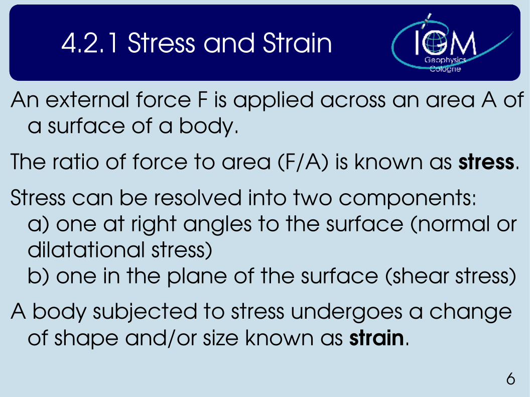
4.2.1 Stress and Strain
An external force F is applied across an area A of a surface of a body.
The ratio of force to area (F/A) is known as stress.
Stress can be resolved into two components: a) one at right angles to the surface (normal or dilatational stress)b) one in the plane of the surface (shear stress)
A body subjected to stress undergoes a change of shape and/or size known as strain.
7
Stress and Strain
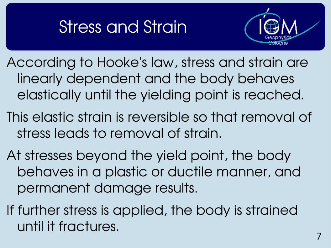
According to Hooke's law, stress and strain are linearly dependent and the body behaves elastically until the yielding point is reached.
This elastic strain is reversible so that removal of stress leads to removal of strain.
At stresses beyond the yield point, the body behaves in a plastic or ductile manner, and permanent damage results.
If further stress is applied, the body is strained until it fractures.
8
Stress and Strain
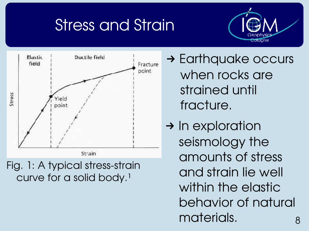
Fig. 1: A typical stressstrain curve for a solid body.¹
→ Earthquake occurs when rocks are strained until fracture.
→ In exploration seismology the amounts of stress and strain lie well within the elastic behavior of natural materials.
9
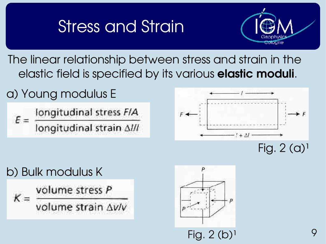
Stress and Strain
a) Young modulus E
b) Bulk modulus K
The linear relationship between stress and strain in the elastic field is specified by its various elastic moduli.
Fig. 2 (a)¹
Fig. 2 (b)¹
10
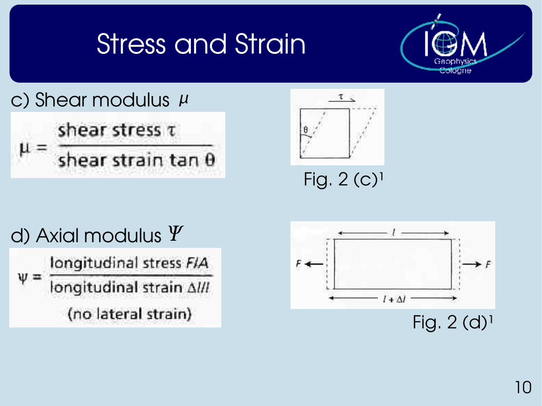
Stress and Strain
c) Shear modulus
d) Axial modulus
Fig. 2 (c)¹
Fig. 2 (d)¹
11
4.2.2 Types of Seismic Waves
Seismic waves are parcels of elastic strain energy that propagate from a seismic source such as an earthquake or an explosion.
The strains associated with the passage of a seismic pulse may be assumed to be elastic (except in the vicinity of the source!)
The propagation of seismic pulses is determined by the elastic moduli and densities of the materials through which they pass.
There are two groups of seismic waves: body waves and surface waves.
12
4.2.2.1 Body waves
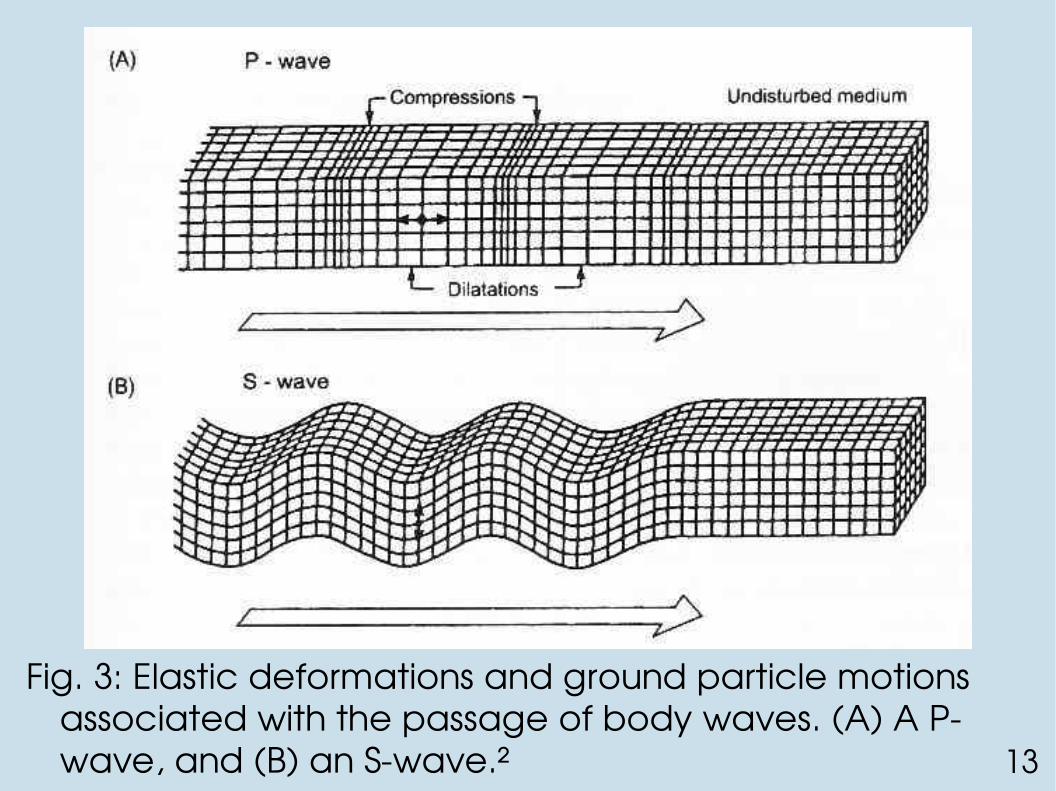
● Pwave (longitudinal, primary or compressional wave)Material particles oscillate about a fixed point in the direction of wave propagation by compressional and dilatational strain.
● Swave (transverse, secondary or shear wave)Particle motion is at right angles to the direction of wave propagation and occurs by pure strain.
Fig. 3: Elastic deformations and ground particle motions associated with the passage of body waves. (A) A Pwave, and (B) an Swave.² 13
14
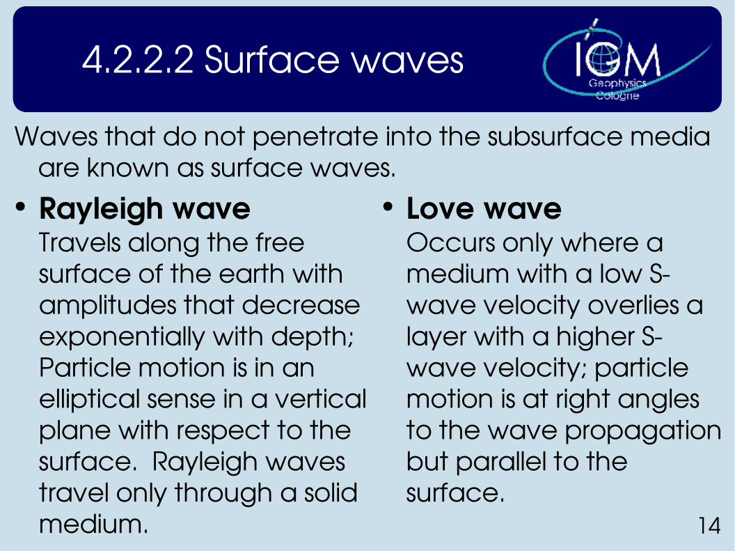
4.2.2.2 Surface waves
● Rayleigh waveTravels along the free surface of the earth with amplitudes that decrease exponentially with depth; Particle motion is in an elliptical sense in a vertical plane with respect to the surface. Rayleigh waves travel only through a solid medium.
● Love waveOccurs only where a medium with a low Swave velocity overlies a layer with a higher Swave velocity; particle motion is at right angles to the wave propagation but parallel to the surface.
Waves that do not penetrate into the subsurface media are known as surface waves.
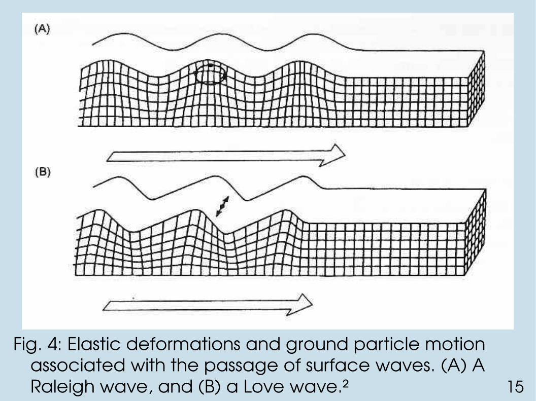
Fig. 4: Elastic deformations and ground particle motion associated with the passage of surface waves. (A) A Raleigh wave, and (B) a Love wave.² 15
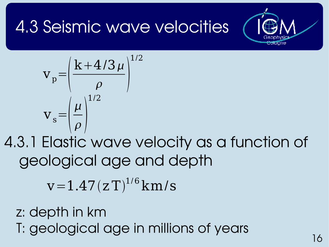
4.3 Seismic wave velocities
v p= k4 /3 1/2
v s= 1/2
4.3.1 Elastic wave velocity as a function of geological age and depth
v=1.47 zT1/6km /s
z: depth in kmT: geological age in millions of years
16
17
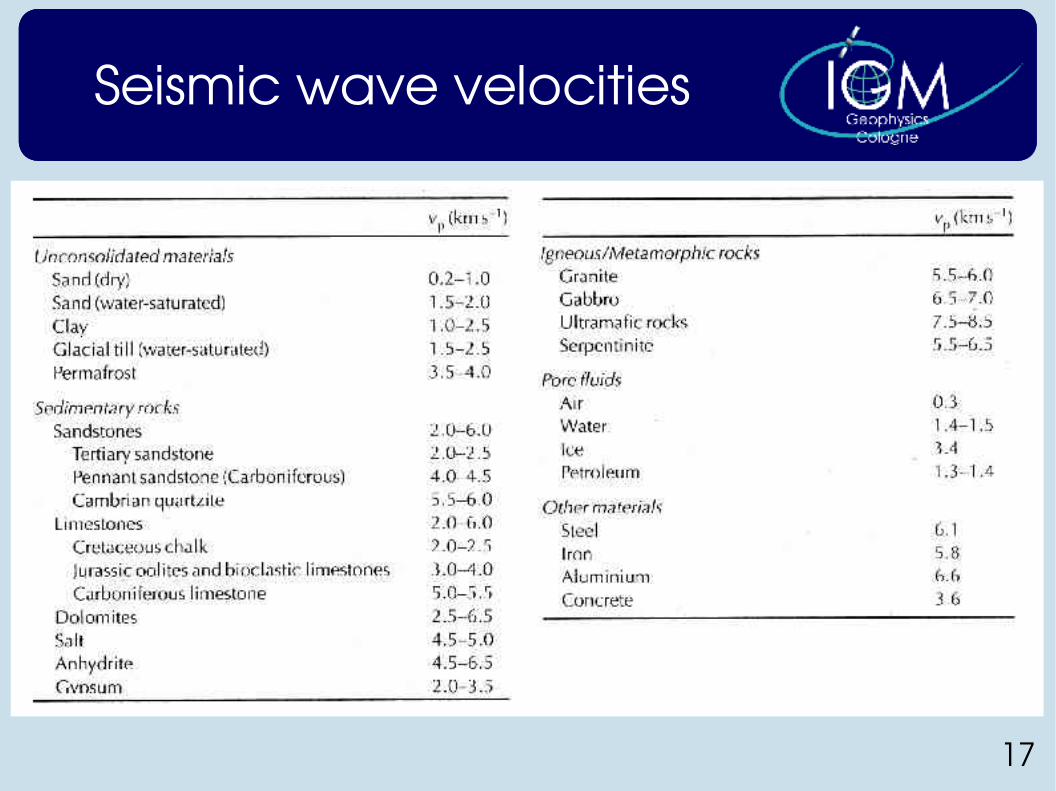
Seismic wave velocities
18
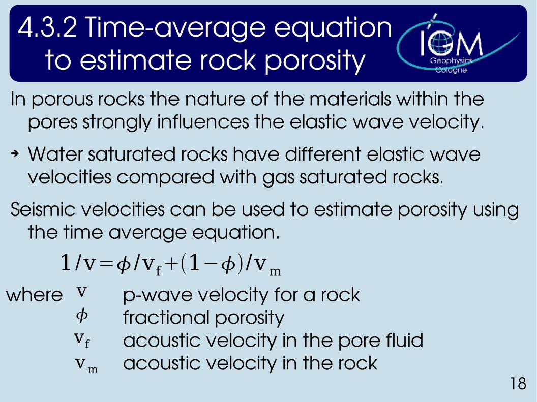
4.3.2 Timeaverage equation to estimate rock porosity
In porous rocks the nature of the materials within the pores strongly influences the elastic wave velocity.
➔ Water saturated rocks have different elastic wave velocities compared with gas saturated rocks.
Seismic velocities can be used to estimate porosity using the time average equation.
1 /v=/vf1−/vmwhere pwave velocity for a rock
fractional porosityacoustic velocity in the pore fluid
acoustic velocity in the rock
vvfvm
19
4.4 Ray paths in layered media
At an interface between two rock layers there is generally a change in propagation velocity resulting from the difference in physical properties of the two layers.
At such an interface, the energy within an incident seismic pulse is partitioned into transmitted and reflected pulses.
The relative amplitudes of the transmitted and reflected pulses depend on the velocities (v) and densities ( ) and the angle of incidence.
20
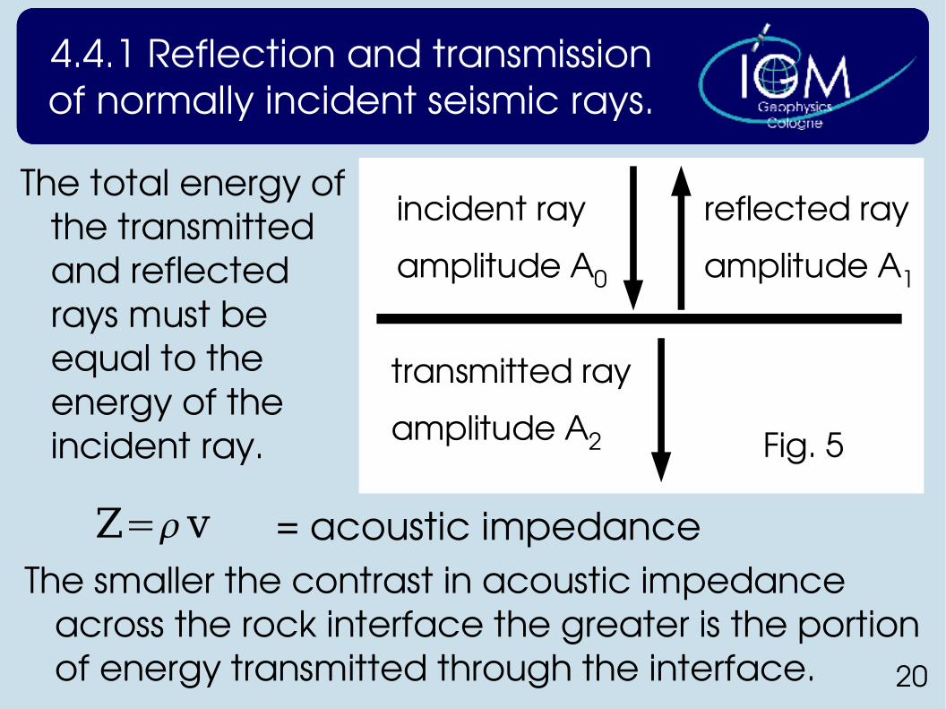
incident ray
amplitude A0
transmitted ray
amplitude A2
reflected ray
amplitude A1
Fig. 5
4.4.1 Reflection and transmission of normally incident seismic rays.
The total energy of the transmitted and reflected rays must be equal to the energy of the incident ray.
Z=v = acoustic impedanceThe smaller the contrast in acoustic impedance
across the rock interface the greater is the portion of energy transmitted through the interface.
21
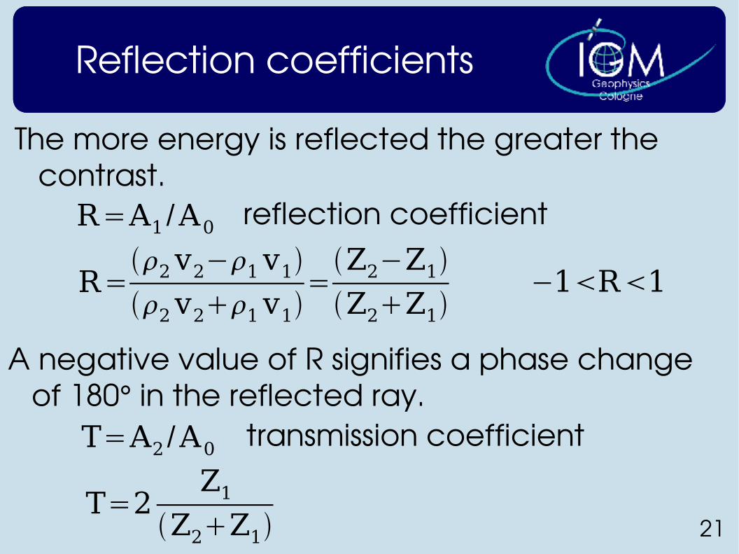
Reflection coefficients
The more energy is reflected the greater the contrast.R=A1 /A0 reflection coefficient
R=2v2−1v12v21v1
=Z2−Z1Z2Z1
−1R1
A negative value of R signifies a phase change of 180° in the reflected ray.
T=A2 /A0 transmission coefficient
T=2Z1
Z2Z1
22
4.4.2 Reflection and refraction of obliquely incident rays
In the case of incident waves reflected and transmitted waves are generated as described in the case of normal incidence.
When a Pwave is incident at an oblique angle on a plane surface, four types of waves are generated:
● reflected and transmitted Pwaves● reflected and transmitted Swaves
23
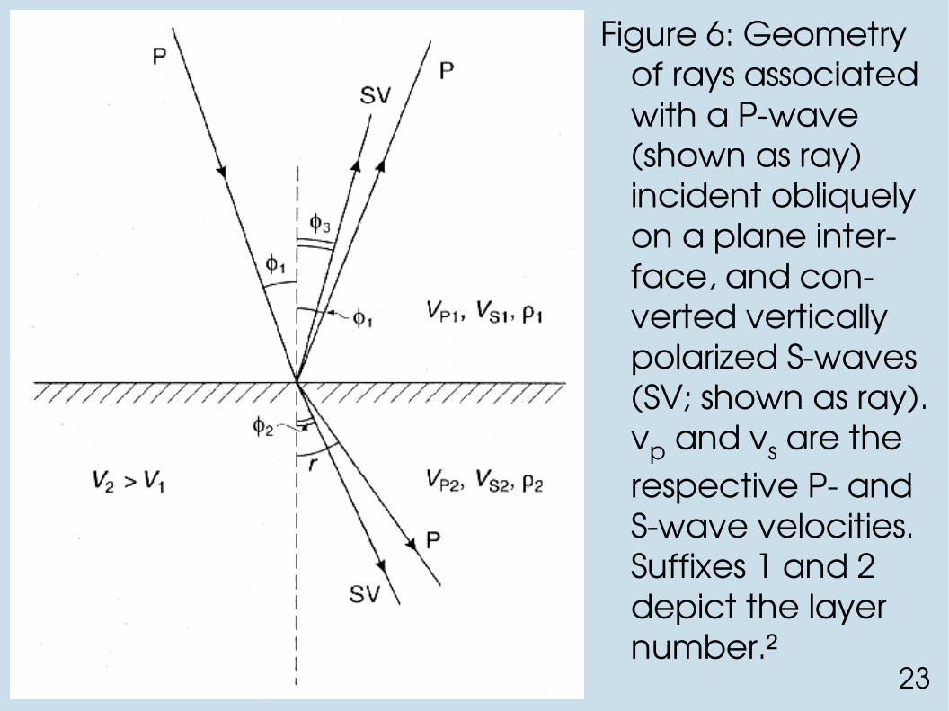
Figure 6: Geometry of rays associated with a Pwave (shown as ray) incident obliquely on a plane interface, and converted vertically polarized Swaves (SV; shown as ray). vp and vs are the respective P and Swave velocities. Suffixes 1 and 2 depict the layer number.²
24
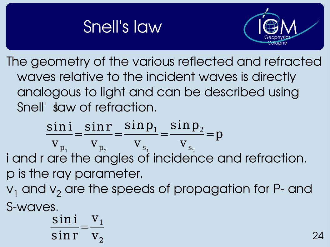
Snell's law
The geometry of the various reflected and refracted waves relative to the incident waves is directly analogous to light and can be described using Snell's law of refraction.
sin iv p1
=sinrv p2
=sinp1v s1
=sinp2v s2
=p
i and r are the angles of incidence and refraction.p is the ray parameter. v1 and v2 are the speeds of propagation for P and Swaves.
sin isinr
=v1v2
25
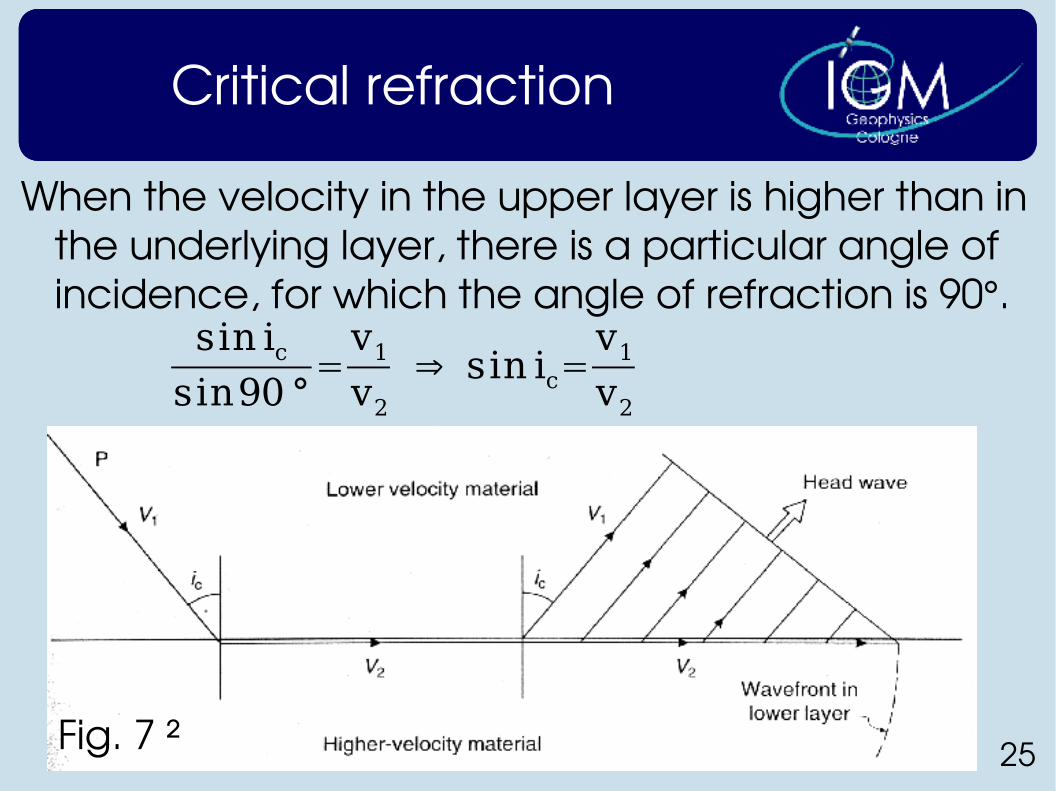
Critical refraction
When the velocity in the upper layer is higher than in the underlying layer, there is a particular angle of incidence, for which the angle of refraction is 90°.
Fig. 7 ²
sin icsin90 °
=v1v2
⇒ sin ic=v1v2
26
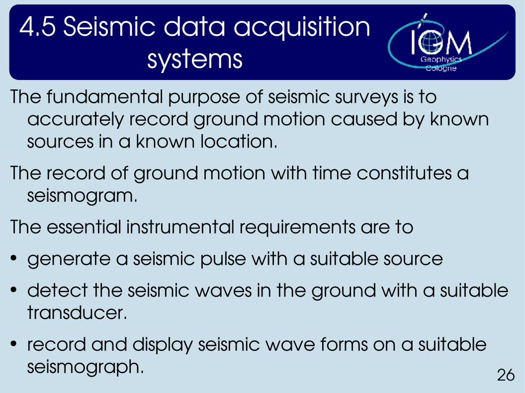
4.5 Seismic data acquisition systems
The fundamental purpose of seismic surveys is to accurately record ground motion caused by known sources in a known location.
The record of ground motion with time constitutes a seismogram.
The essential instrumental requirements are to● generate a seismic pulse with a suitable source● detect the seismic waves in the ground with a suitable
transducer.● record and display seismic wave forms on a suitable
seismograph.
27
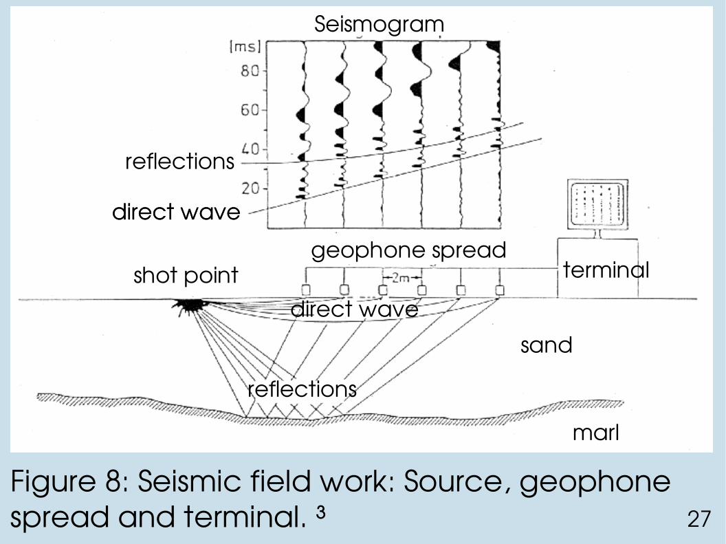
Seismogram
reflections
direct wave
direct wavedirect wave
reflections
geophone spread
sand
marl
Figure 8: Seismic field work: Source, geophone spread and terminal. ³
shot point terminal
28
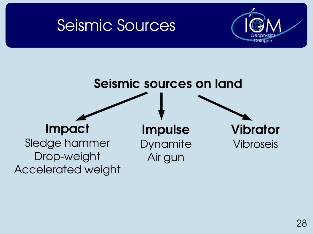
Seismic Sources
Seismic sources on land
ImpactSledge hammer
DropweightAccelerated weight
ImpulseDynamite
Air gun
VibratorVibroseis
29
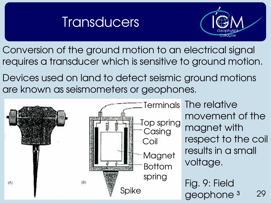
Transducers
Conversion of the ground motion to an electrical signal requires a transducer which is sensitive to ground motion.
Devices used on land to detect seismic ground motions are known as seismometers or geophones.
The relative movement of the magnet with respect to the coil results in a small voltage.
Fig. 9: Field geophone ³
Terminals
Top springCasingCoil
MagnetBottomspring
Spike
30
4.7 Seismic reflection surveying
4.7.1 Introduction and general considerations
Seismic reflection is the most widely used geophysical technique. Important details about the geometry of the structure and about the physical properties can be derived.
Its predominant applications are hydrocarbon exploration and research into crustal structure with depths of penetration of several kilometers.
31
Introduction and general considerations
Since 1980 the method has been applied increasingly to engineering and environmental investigations (< 200 m)
➔ hydrogeological studies of aquifers➔ shallow coal exploration➔ preconstruction ground investigations for pipe,
cables and sewerage schemes
32
Introduction and general considerations
The essence of the seismic reflection technique is to measure the time taken for a seismic wave to travel from a source down into the ground where it is reflected back to the surface and then detected at a receiver.
The time is known as the two way travel time (TWTT).
The most important problem in seismic reflection surveying is the translation of TWTT to depth.
While travel times are measured, the one parameter, that most affects the conversation of to depth is seismic velocity.
➔ two unknowns (depth + velocity)
33
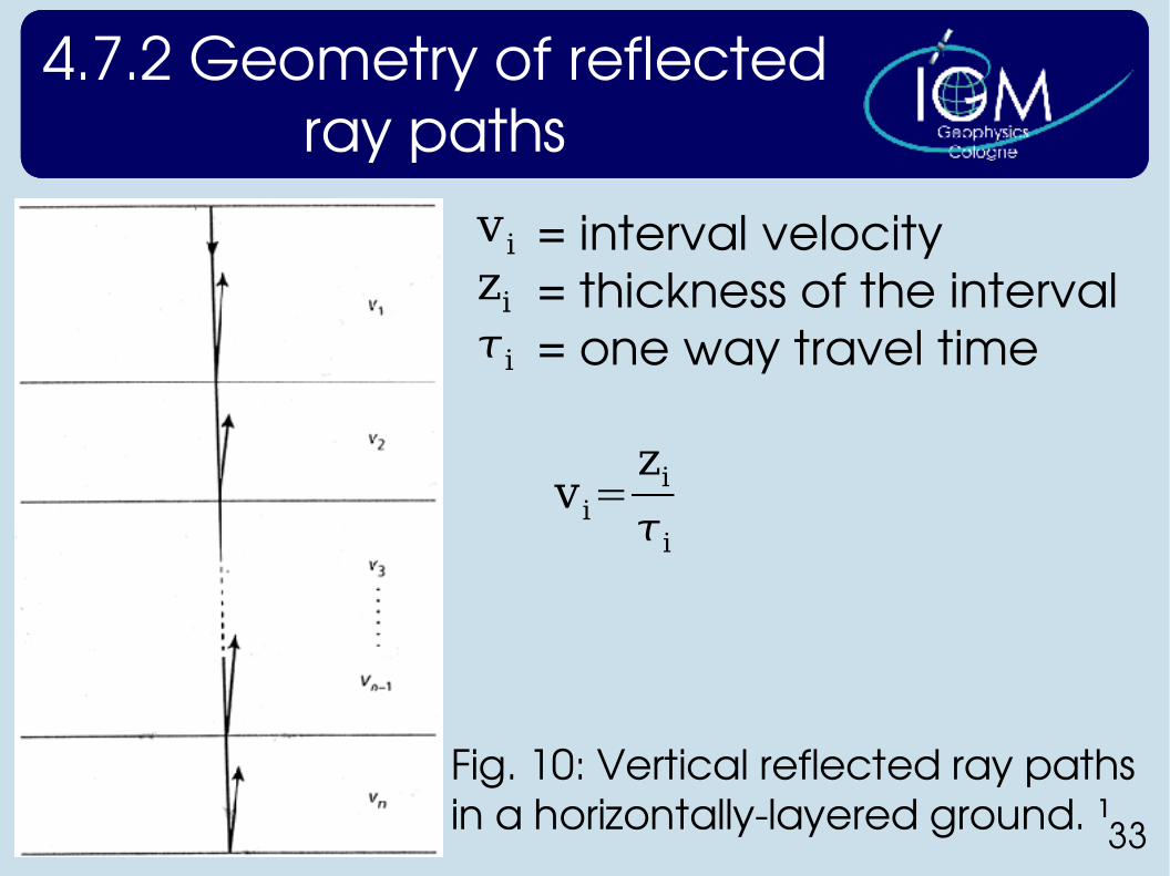
4.7.2 Geometry of reflected ray paths
Fig. 10: Vertical reflected ray paths in a horizontallylayered ground. ¹
vizii
= interval velocity= thickness of the interval= one way travel time
vi=zii
34
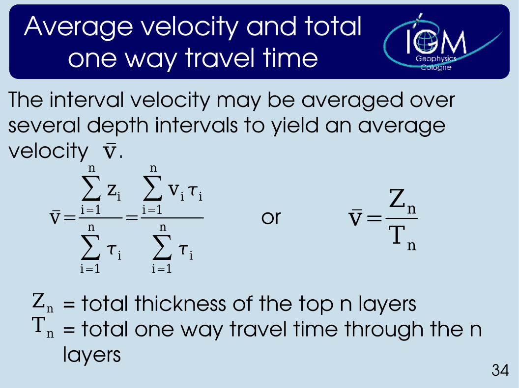
Average velocity and total one way travel time
The interval velocity may be averaged over several depth intervals to yield an average velocity .v
v=∑i=1
n
zi
∑i=1
n
i
=∑i=1
n
v i i
∑i=1
n
i
or v=ZnTn
ZnTn
= total thickness of the top n layers= total one way travel time through the n layers
35
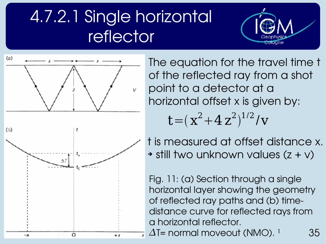
4.7.2.1 Single horizontal reflector
Fig. 11: (a) Section through a single horizontal layer showing the geometry of reflected ray paths and (b) timedistance curve for reflected rays from a horizontal reflector. T= normal moveout (NMO). ¹
The equation for the travel time t of the reflected ray from a shot point to a detector at a horizontal offset x is given by:
t=x24z21/2 /v
t is measured at offset distance x.➔ still two unknown values (z + v)
36
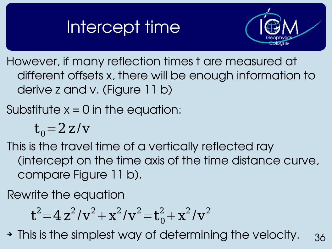
Intercept time
However, if many reflection times t are measured at different offsets x, there will be enough information to derive z and v. (Figure 11 b)
Substitute x = 0 in the equation:
t0=2z /vThis is the travel time of a vertically reflected ray
(intercept on the time axis of the time distance curve, compare Figure 11 b).
Rewrite the equation
t2=4z2 /v2x2 /v2=t02x2 /v2
➔ This is the simplest way of determining the velocity.
37
Velocity determination
➔ Plot t2 against x2
The graph will produce a straight line of slope 1/v2.The intercept on the time axis will give the vertical two way travel time, t0 , from which the depth to the reflector can be found.
This method is unsatisfactory, since the values of x are restricted.
A much better method of determining velocity is by considering the increase of reflected travel time with offset distance, the moveout.
38
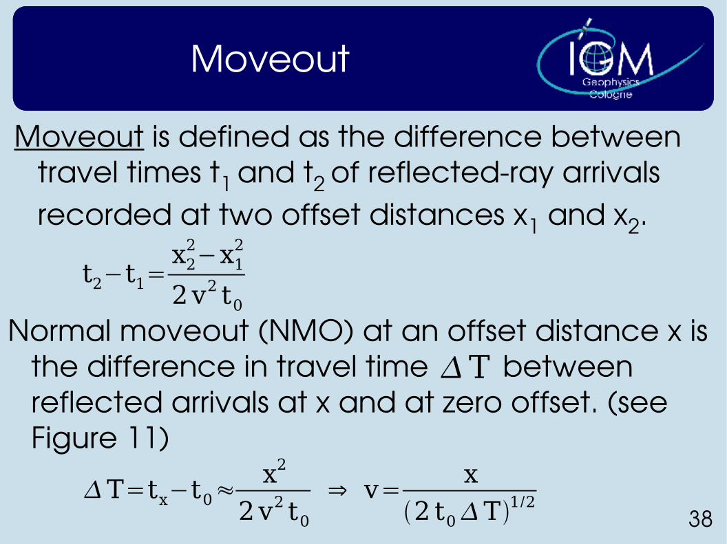
Moveout
Moveout is defined as the difference between travel times t1 and t2 of reflectedray arrivals recorded at two offset distances x1 and x2.
t2−t1=x22−x1
2
2v2 t0Normal moveout (NMO) at an offset distance x is
the difference in travel time between reflected arrivals at x and at zero offset. (see Figure 11)
T
T=tx−t0≈x2
2v2 t0⇒ v= x
2 t0T1/2
39
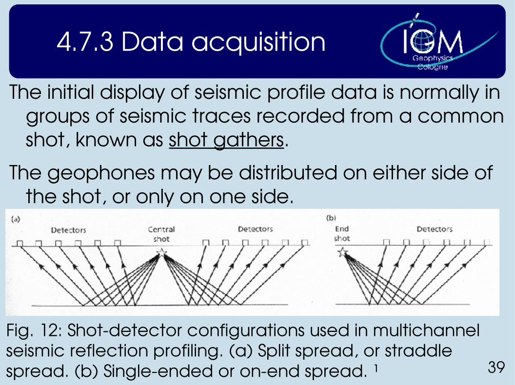
4.7.3 Data acquisition
Fig. 12: Shotdetector configurations used in multichannel seismic reflection profiling. (a) Split spread, or straddle spread. (b) Singleended or onend spread. ¹
The initial display of seismic profile data is normally in groups of seismic traces recorded from a common shot, known as shot gathers.
The geophones may be distributed on either side of the shot, or only on one side.
40
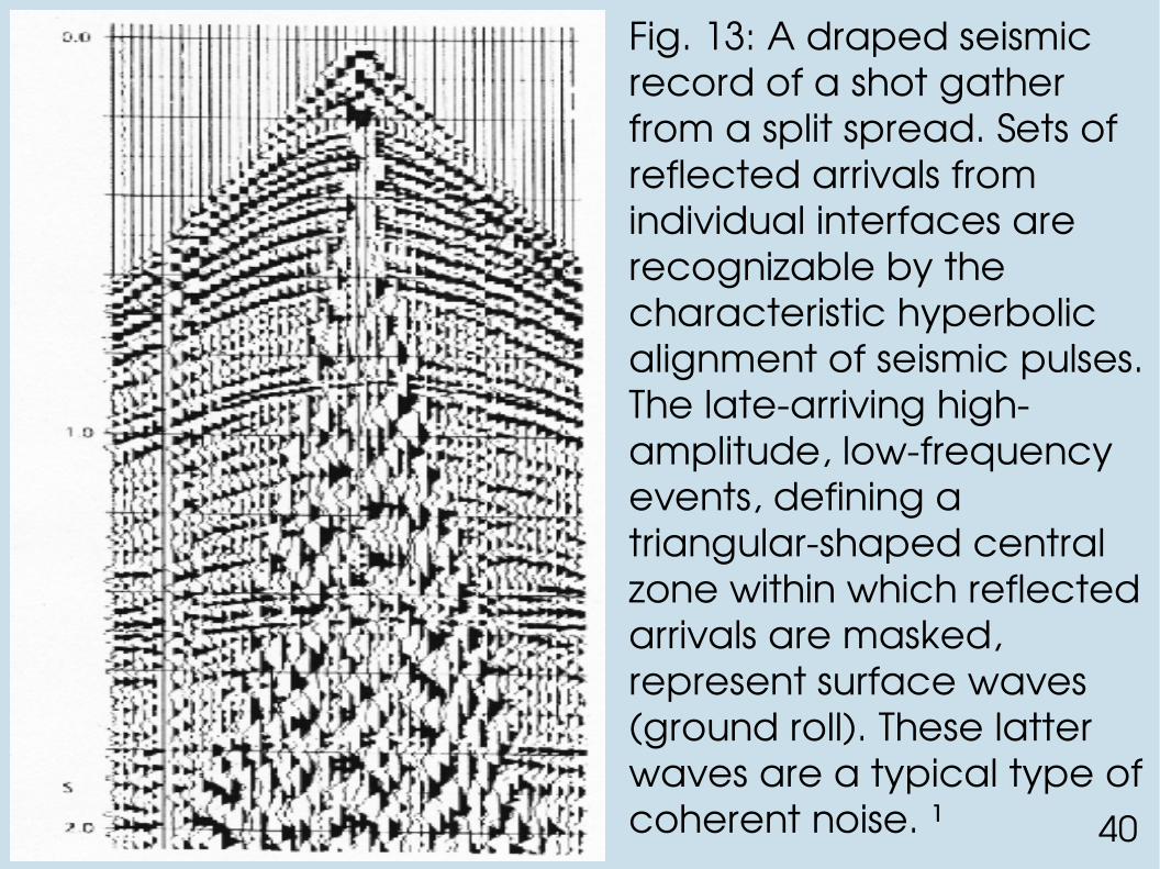
Fig. 13: A draped seismic record of a shot gather from a split spread. Sets of reflected arrivals from individual interfaces are recognizable by the characteristic hyperbolic alignment of seismic pulses. The latearriving highamplitude, lowfrequency events, defining a triangularshaped central zone within which reflected arrivals are masked, represent surface waves (ground roll). These latter waves are a typical type of coherent noise. ¹
41
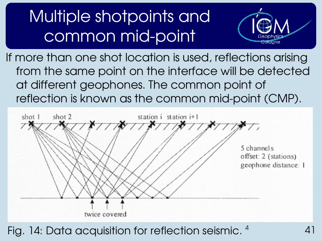
Multiple shotpoints and common midpoint
If more than one shot location is used, reflections arising from the same point on the interface will be detected at different geophones. The common point of reflection is known as the common midpoint (CMP).
Fig. 14: Data acquisition for reflection seismic. 4
42
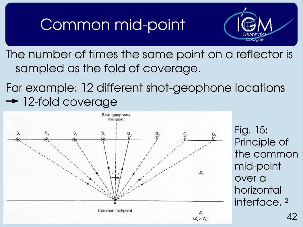
Common midpoint
The number of times the same point on a reflector is sampled as the fold of coverage.
For example: 12 different shotgeophone locations 12fold coverage
Fig. 15: Principle of the common midpoint over a horizontal interface. ²
43
Common midpoint gather
The CMP gather lies in the heart of seismic processing for two main reasons:
1) The variation of travel time with offset, the moveout will depend only on the velocity of the subsurface layers (horizontal uniform layers).
➔ The subsurface velocity can be derived.
2) The reflected seismic energy is usually very weak. It is imperative to increase the signalnoise ratio of most data.
44
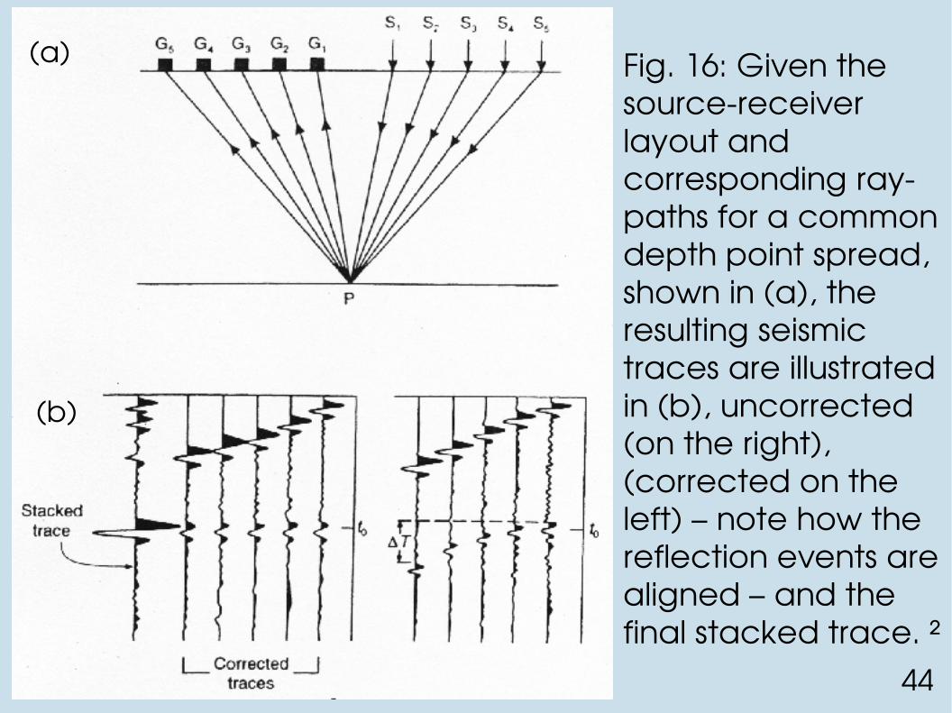
Fig. 16: Given the sourcereceiver layout and corresponding raypaths for a common depth point spread, shown in (a), the resulting seismic traces are illustrated in (b), uncorrected (on the right), (corrected on the left) – note how the reflection events are aligned – and the final stacked trace. ²
(a)
(b)
45
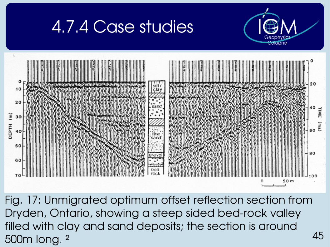
4.7.4 Case studies
Fig. 17: Unmigrated optimum offset reflection section from Dryden, Ontario, showing a steep sided bedrock valley filled with clay and sand deposits; the section is around 500m long. ²
46
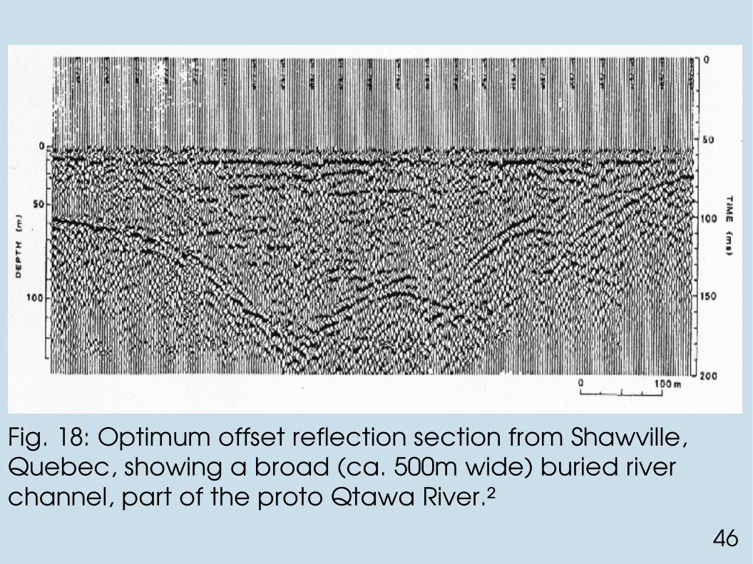
Fig. 18: Optimum offset reflection section from Shawville, Quebec, showing a broad (ca. 500m wide) buried river channel, part of the proto Qtawa River.²
47
4.8 Seismic refraction surveying
The seismic refraction surveying method uses seismic energy that returns to the surface after traveling through the ground along refracted ray paths.
The most commonly derived geophysical parameter is the seismic velocity of the layers present.
A number of geotechnical parameters can be derived from seismic velocity.
In addition to the more conventional engineering applications of foundation studies for dams and major buildings, seismic refraction is increasingly being used in hydrogeological investigations to determine saturated aquifer thickness, weathered fault zones.
48
4.8.1 General Principles
The refraction method is dependent upon there being an increase in velocity with depth.
The direction of travel of a seismic wave changes on entry into a new medium.
The amount of change of direction is governed by the contrast in seismic velocity across the boundary according to Snell's law.
49
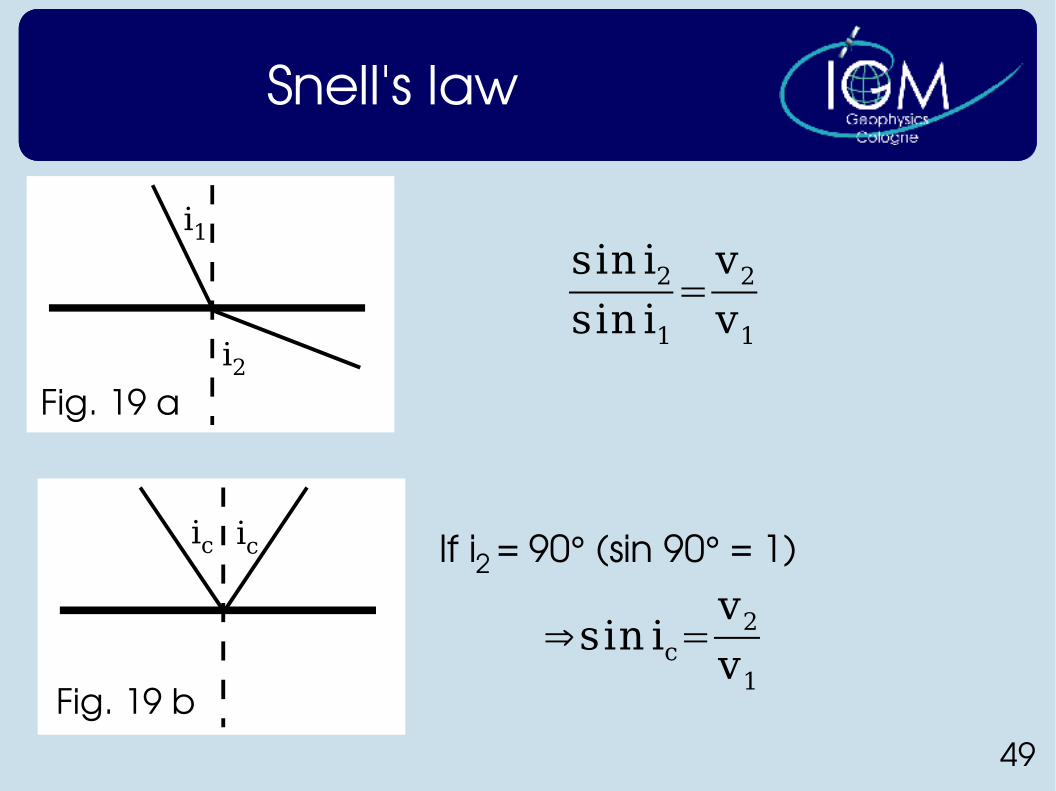
Snell's law
i1
i2
sin i2sin i1
=v2v1
If i2 = 90° (sin 90° = 1)ic ic
⇒sin ic=v2v1
Fig. 19 a
Fig. 19 b
50
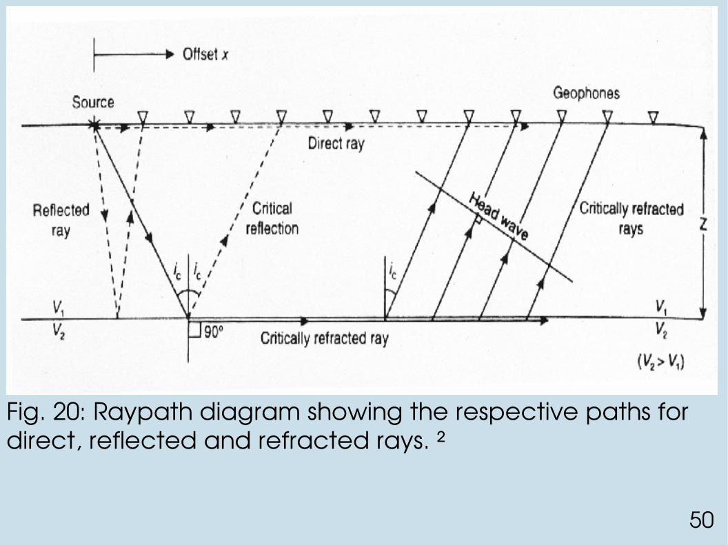
Fig. 20: Raypath diagram showing the respective paths for direct, reflected and refracted rays. ²
51
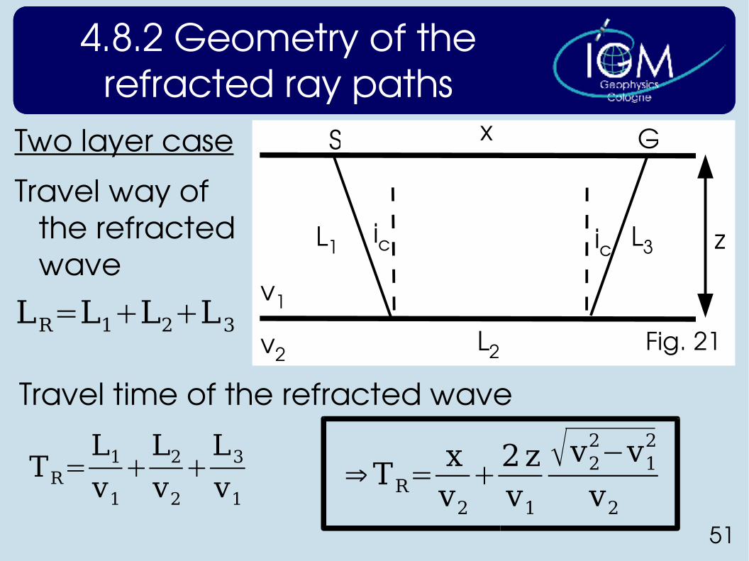
4.8.2 Geometry of the refracted ray paths
Two layer case
Travel way of the refracted wave
Fig. 21v2
v1
L1
L2
L3ic ic
xS G
z
LR=L1L2L3
Travel time of the refracted wave
TR=L1v1
L2v2
L3v1
⇒TR=xv2
2zv1
v22−v12v2
52
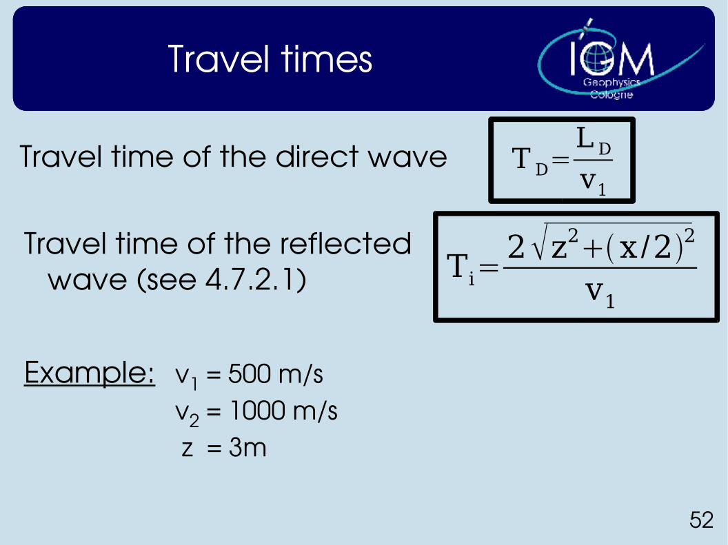
Travel times
Travel time of the direct wave T D=L D
v1
Travel time of the reflected wave (see 4.7.2.1) Ti=
2z2x /22
v1
T D=L D
v1
Example: v1 = 500 m/sv2 = 1000 m/s z = 3m
53
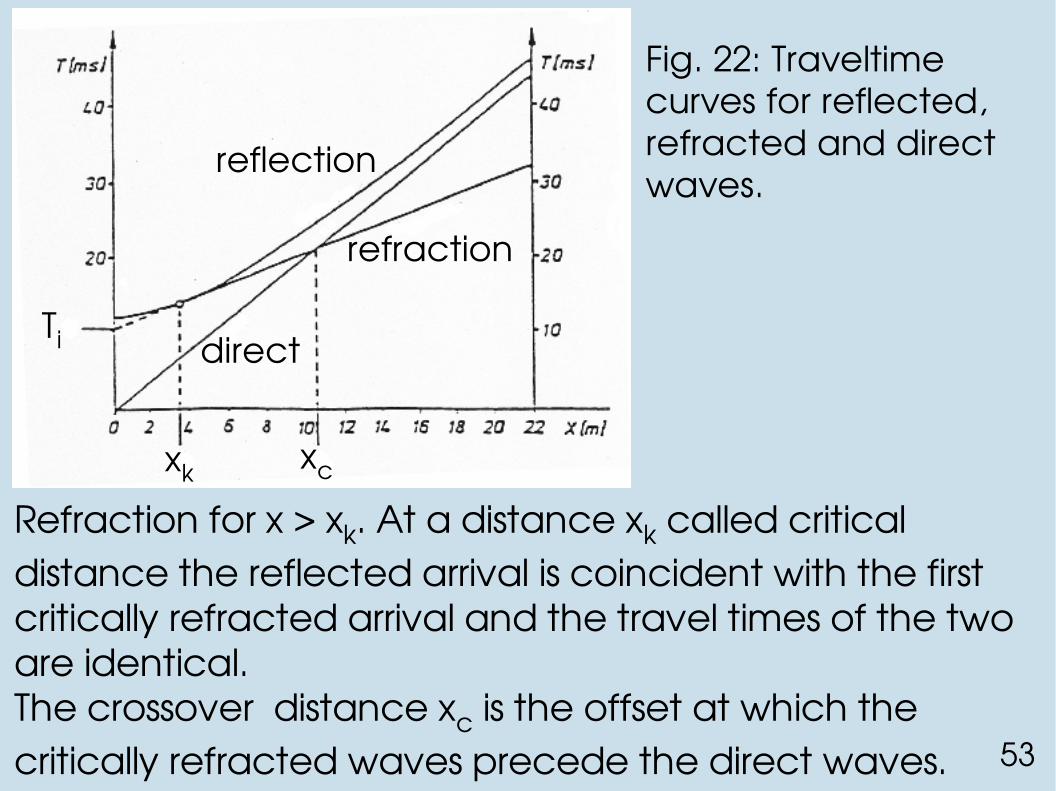
Refraction for x > xk. At a distance xk called critical distance the reflected arrival is coincident with the first critically refracted arrival and the travel times of the two are identical.The crossover distance xc is the offset at which the critically refracted waves precede the direct waves.
Fig. 22: Traveltime curves for reflected, refracted and direct waves.
xk xc
direct
refraction
reflection
Ti
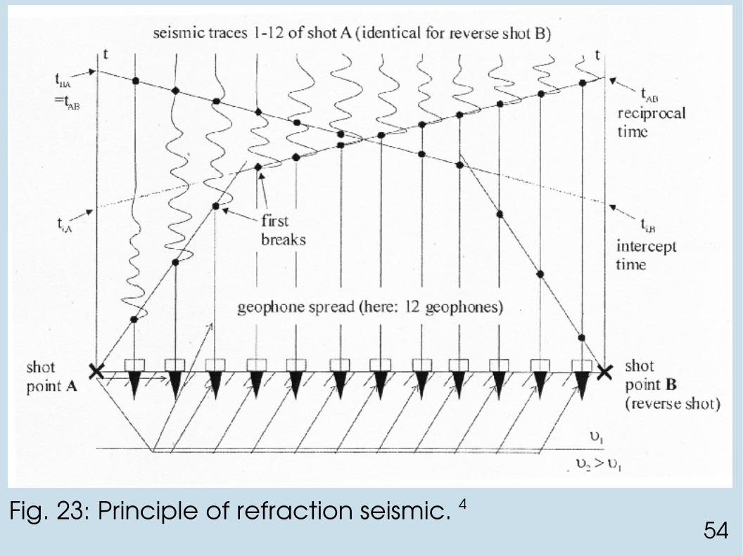
54Fig. 23: Principle of refraction seismic. 4
55
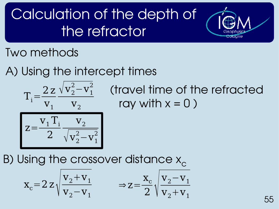
Calculation of the depth of the refractor
Two methods
A) Using the intercept times
Ti=2zv1
v22−v12v2
(travel time of the refracted ray with x = 0 )
z=v1Ti2
v2
v22−v12
B) Using the crossover distance xc
xc=2z v2v1v2−v1⇒z=
xc2 v2−v1v2v1
56
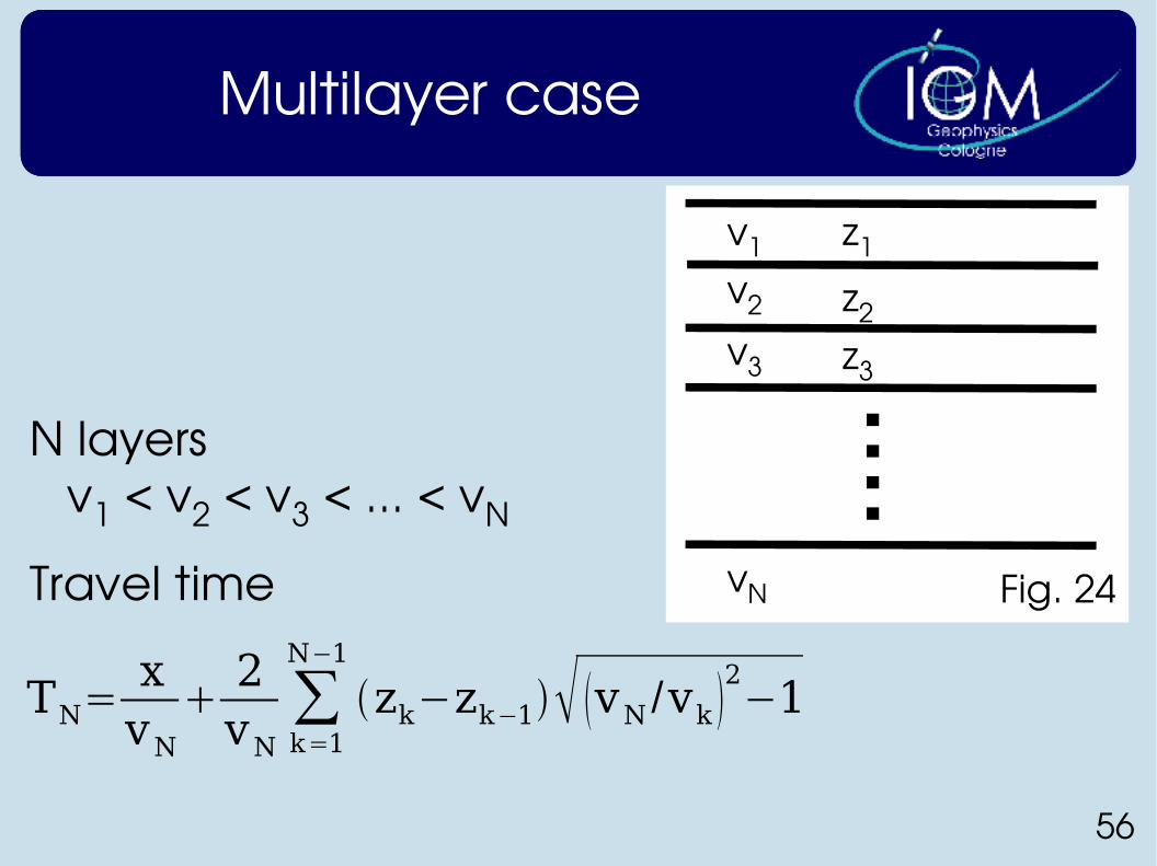
Multilayer case
N layersv1 < v2 < v3 < ... < vN
Travel time
v1
v2
v3
vN
z1
z2
z3
Fig. 24
TN=xvN
2vN
∑k=1
N−1
zk−zk−1 vN /vk 2−1
57
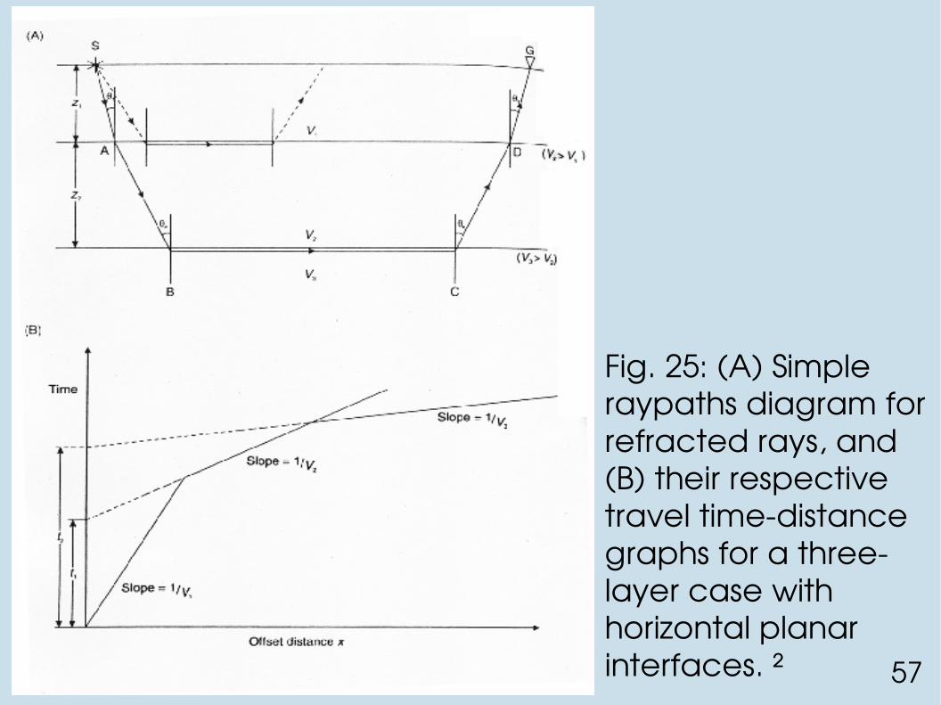
Fig. 25: (A) Simple raypaths diagram for refracted rays, and (B) their respective travel timedistance graphs for a threelayer case with horizontal planar interfaces. ²
58
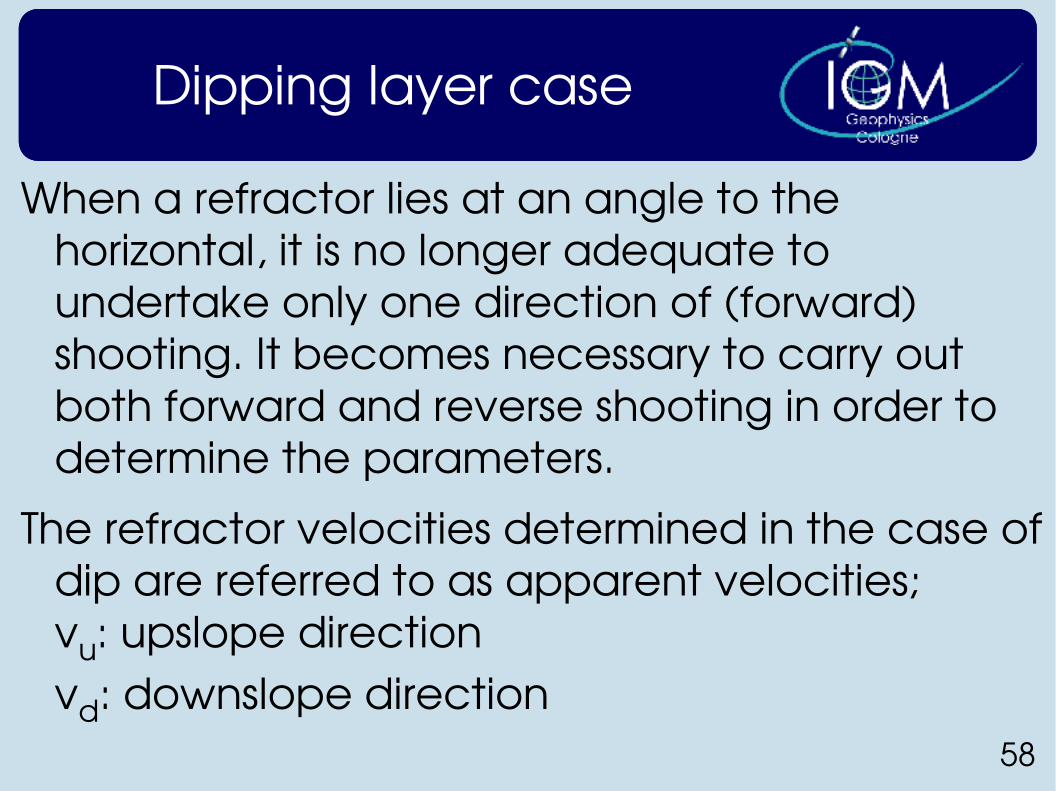
Dipping layer case
When a refractor lies at an angle to the horizontal, it is no longer adequate to undertake only one direction of (forward) shooting. It becomes necessary to carry out both forward and reverse shooting in order to determine the parameters.
The refractor velocities determined in the case of dip are referred to as apparent velocities;vu: upslope directionvd: downslope direction
59
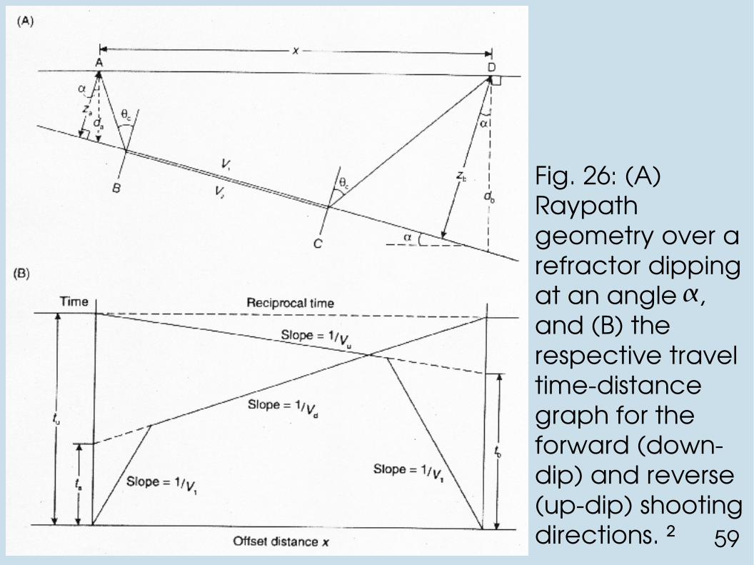
Fig. 26: (A) Raypath geometry over a refractor dipping at an angle , and (B) the respective travel timedistance graph for the forward (downdip) and reverse (updip) shooting directions. ²
60
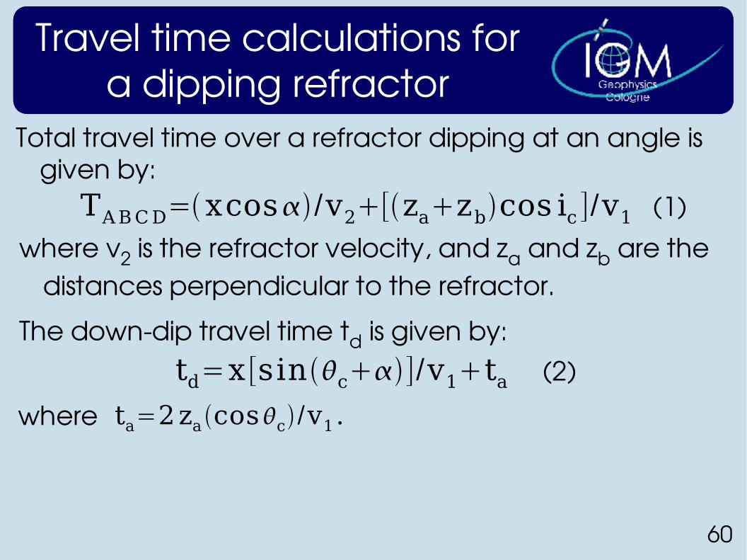
Travel time calculations for a dipping refractor
Total travel time over a refractor dipping at an angle is given by:TABCD=xcos/v2[zazbcos ic ]/v1
where v2 is the refractor velocity, and za and zb are the distances perpendicular to the refractor.
The downdip travel time td is given by:td=x [sinc]/v1ta
where ta=2zacosc /v1 .
(1)
(2)
61
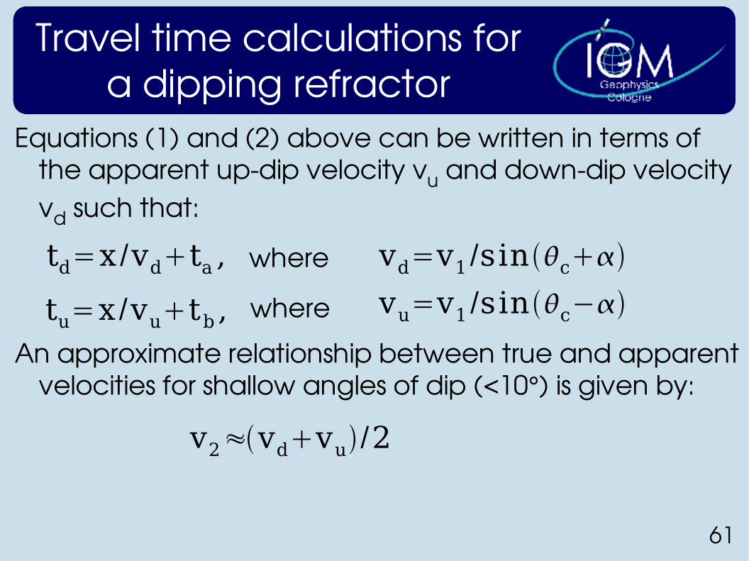
Travel time calculations for a dipping refractor
Equations (1) and (2) above can be written in terms of the apparent updip velocity vu and downdip velocity vd such that:
td=x /vdta ,
tu=x /vutb ,
where
where
vd=v1 /sinc
vu=v1 /sinc−
An approximate relationship between true and apparent velocities for shallow angles of dip (<10°) is given by:
v2≈vdvu /2
62
References
1) Kearey, P., Brooks, M.: An Introduction to Geophysical Exploration, Blackwell, 2002
2) Reynolds, J. M.: An Introduction to Applied and Environmental Geophysics, Wiley, 1998
3) Kirsch, R.: Umweltgeophysik in der Praxis: Untersuchung von Altablagerungen und kontaminierten Standorten, Script
4) Dietrich, P.: Introduction to Applied Geophysics, Script, Sept. 2002