TERM PROJECT

PTE 599 Advanced Production Engineering

DESIGN OF WATER INJECTION SYSTEM FOR OIL AND GAS PRODUCTION USING

PIPESIM STEADY STATE MULTIPHASE FLOW SIMULATOR

Thomas John, Nithin

USC ID: 5988 3597 37

TABLE OF CONTENTS

1. Project Review 1

2. Project Outline 2

3. Calculations & Plots 3

4. Conclusion 15

PROJECT REVIEW

The primary objective of the term project was to design a water injection system for oil and gas

production using PIPESIM Steady State Multiphase Flow Simulator. The PIPESIM Simulator is

used for design and diagnostic analysis of oil and production systems, from initial pore to the final

process. The software delivers the most comprehensive steady state flow assurance workflows

in oil and gas industry, supporting field management and production operations decisions.

Moreover, the software enables optimized well performance through comprehensive modeling of

completion and artificial lift systems. Analysis and optimization of complex production and

injection networks is made facile by PIPESIM Simulator.

Due to the reduction of reservoir pressure after long production hours, it becomes difficult to

produce the remaining oil or gas reserves by natural means. Artificial and gas lift systems have

made it possible to continue production at optimum levels even at rapidly declining reservoir

pressures. In addition to the above, secondary recovery mechanisms, such as; a water injection

system for waterflooding process to improve oil recovery can be utilized. Waterflooding is use of

water injection to increase production from oil reservoirs. The injection of water into the reservoir

increases the reservoir pressure to its initial level and maintains the pressure at that level.

Waterflooding by water injection is all the more advantageous because the water produced along

with oil can easily be separated and re-injected into the reservoir. This ensures safe disposal and

reuse of water; which makes waterflooding one of the least expensive oil recovery mechanisms.

Thus, it is imperative to study more about the waterflooding mechanism by designing an efficient

water injection system.

PROJECT OUTLINE

The water injection system design includes six injection wells and associated pumps to meet the

required production rate. The system is to be designed for 35,400 BPD of water injection. The

following deliverables are required from the system design:

Maximum water injection pressures at the wells

Capacity of pump

Discharge pressure of pump

Number of pump stages required

Maximum horsepower (HP)

Fluid velocity of injection water at each junction joint

Operation costs

In addition to the above, we are also required to determine pressure drop (PD) across each line

based on injection line sizes. The following assumptions were taken into consideration for the

design process:

Specific gravity (SG) of produced water = 1.180

Formation fracture gradient = 0.78 psi/ft.

Safety factor (SF) for wellhead pressure (Pwh) = 100 psi

Electricity cost = 5.15¢ per kWh

Surface temperature = 60 degF

Pipeline roughness = 0.001 in.

Pipeline wall thickness = 0.5 in.

Inner diameter (ID) and type of trunk line = 6 in. Schedule 80

Inner diameter (ID) and type of injection line = 3 in. Schedule 80

Flat terrain, no valleys or mountains

Each well has equal amount of injection fluid

CALCULATIONS

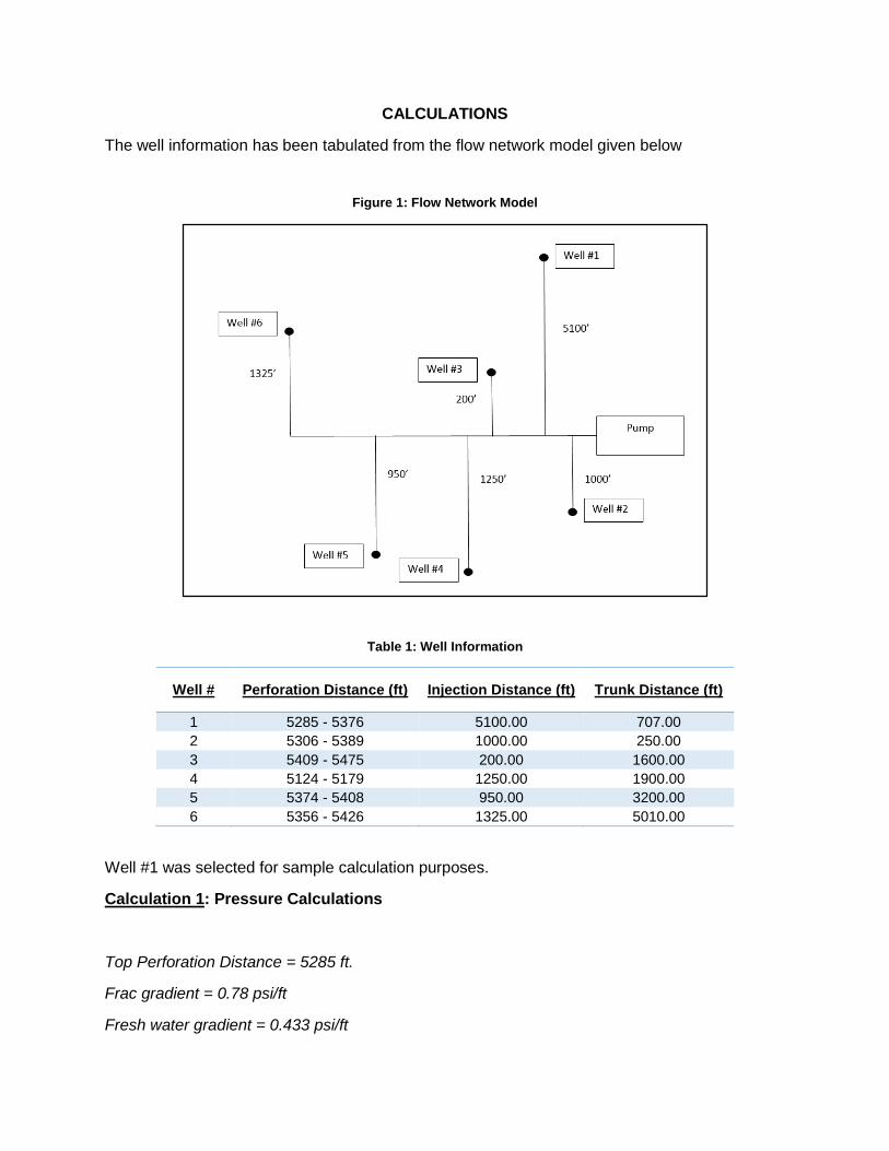
The well information has been tabulated from the flow network model given below

Figure 1: Flow Network Model

Table 1: Well Information

Well # Perforation Distance (ft) Injection Distance (ft) Trunk Distance (ft)

1 5285 - 5376 5100.00 707.00

2 5306 - 5389 1000.00 250.00

3 5409 - 5475 200.00 1600.00

4 5124 - 5179 1250.00 1900.00

5 5374 - 5408 950.00 3200.00

6 5356 - 5426 1325.00 5010.00

Well #1 was selected for sample calculation purposes.

Calculation 1: Pressure Calculations

Top Perforation Distance = 5285 ft.

Frac gradient = 0.78 psi/ft

Fresh water gradient = 0.433 psi/ft

Specific Gravity of water = 1.18

Fracture Pressure = Frac Gradient x Top Perf Distance

Pf = 0.78 x 5285 = 4122.30 psi

Hydrostatic Pressure = Specific Gravity x Fresh water gradient x Top Perf Distance

Ph = 1.18 x 0.433 x 5285 = 2700.32 psi

Wellhead Pressure = Fracture Pressure – Hydrostatic Pressure

Pwh’ = 4122.30 – 2700.32 = 1421.98 psi

Wellhead Pressure assuming a safety factor of 100 psi

Pwh = 1421.98 – 100 = 1321.98 psi

The results are tabulated in Table 2.

Table 2: Wellhead Pressure Calculation

Well # Frac Pressure,

Pf (psi) Hydrostatic

Pressure, Ph (psi) Wellhead

Pressure, Pwh (psi)

1 4122.3 2700.32 1321.98

2 4138.68 2711.05 1327.63

3 4219.02 2763.67 1355.35

4 3996.72 2618.05 1278.67

5 4191.72 2745.79 1345.93

6 4177.68 2736.59 1341.09

Calculation 2: Injection Line Calculations

For injection line calculations, the overall pump flow rate was equally divided among the six wells

to calculate pressure difference and trunk-injection junction pressures for each well.

Figure 2: Viscosity as a function of Temperature

Table 2: Schedule N80 Pipe Data

Injection Rate = 5900 BPD

Inner diameter of injection line = 2.90 inches = 0.2417 feet (From Table 3)

Viscosity = 1.129 cP (From Figure 2)

Water Density = 62.4 ppg

Specific Gravity of produced fluid = γf = 1.18

Fluid Velocity = 4 × q

inj × 5.615

π × d2 × 86400

v f = 4 × 5900 × 5.615

π × 0.24172× 86400

= 8.36 ft/ sec

Reynold's Number =

1488 × d × v f× ρw

× γf

μ

NRe =1488 × 0.2417 × 8.36 × 62.4×1.18

1.129 = 196144.98

Friction Factor = 1

√fm

= 1.14-2 log (eD+21.25

NRe0.90

)

eD = Relative Pipe Roughness = Absolute roughness / D = (0.001 / 2.90)

1

√fm = 1.14-2 log ( 0.001

2.90⁄ +21.25

196144.980.90

)

fm = 0.0181

The pressure difference between wellhead pressure and junction pressure is given by:

∆P = 0.433 × Lsinθ + 1.15×10-5

×fm × γ

f × q

inj× L

D5

Since there is no elevation, θ is taken as 0 and hence equation reduces to;

∆P = 1.15×10-5

×fm × γ

f × q

inj× L

D5

∆P = 1.15×10-5

×0.0181 ×1.18 ×5900× 5100

2.905

= 212.42

Junction Pressure = Wellhead Pressure + DeltaP

Pressurejuction = 1321.98 + 212.42 = 1534.40 psi

The results are tabulated in Table 4.

Table 4: Junction Pressure Calculation

Well # Length,

L (ft)

Injection Rate, q_inj

(BPD)

Wellhead Pressure, Pwh (psi)

Fluid Velocity, v (ft/s)

Reynolds Number,

NRe

Friction Factor,

fm

DeltaP (psi)

Junction Pressure, Pj (psi)

1 5100.00 5900.00 1321.98 8.36 196144.98 0.0181 212.42 1534.40

2 1000.00 5900.00 1327.63 8.36 196144.98 0.0181 41.65 1369.28

3 200.00 5900.00 1355.35 8.36 196144.98 0.0181 8.33 1363.68

4 1250.00 5900.00 1278.67 8.36 196144.98 0.0181 52.06 1330.73

5 950.00 5900.00 1345.93 8.36 196144.98 0.0181 39.57 1385.50

6 1325.00 5900.00 1341.09 8.36 196144.98 0.0181 55.19 1396.28

Calculation 3: Trunk Line Calculations

For trunk line calculations, the cumulative injection for each well was taken into consideration.

The inner diameter (ID) of trunk line was determined to be 5.761 inches (0.4801 feet) from Table

3.

Similar equations for injection line calculations were used to obtain results for trunk line; displayed

in Table 5.

Table 5: Trunk Line Calculations

Well #

Length, L (ft)

Cumulative Injection

Rate, qcinj (BPD)

Wellhead Pressure, Pwh (psi)

Fluid Velocity, v (ft/s)

Reynolds Number,

NRe

Friction Factor,

fm

DeltaP/section (psi)

DeltaP to each section

(psi)

2 457 35400.00 1321.98 12.72 592418.46 0.0150 18.39 18.39

1 250 29500.00 1327.63 10.60 493682.05 0.0153 7.10 25.49

3 893 23600.00 1355.35 8.48 394945.64 0.0156 16.59 42.09

4 300 17700.00 1278.67 6.36 296209.23 0.0161 3.24 45.32

5 1300 11800.00 1345.93 4.24 197472.82 0.0170 6.56 51.89

6 1810 5900.00 1341.09 2.12 98736.41 0.0189 2.54 54.43

Calculation 4: Discharge Pressure Calculation

Discharge pressure can be calculates by:

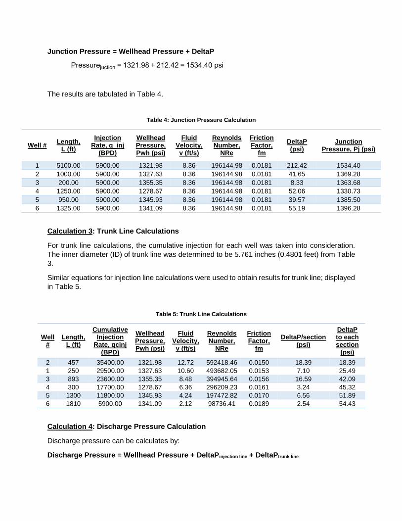
Discharge Pressure = Wellhead Pressure + DeltaPinjection line + DeltaPtrunk line

Discharge Pressure at well #1 = 1321.98 + 212.42 + 25.49 = 1559.89 psi

The results are tabulated in Table 6.

Table 6: Discharge Pressure Calculations

Well # Wellhead Pressure,

Pwh (psi) DeltaP, injection

(psi) DeltaP, trunk (psi)

Discharge Pressure, Pd (psi)

1 1321.98 212.42 25.49 1559.89

2 1327.63 41.65 18.39 1387.67

3 1355.35 8.33 42.09 1405.77

4 1278.67 52.06 45.32 1376.05

5 1345.93 39.57 51.89 1437.39

6 1341.09 55.19 54.43 1450.71

The maximum value of discharge pressure is taken as 1559.89, corresponding to well #1. The discharge pressure should not exceed the maximum injection pressure for each well.

From the maximum discharge pressure, we can calculate actual injection pressure for each well.

Actual Injection Pressure = Maximum discharge pressure – DeltaPtotal

Actual Injection Pressure = 1560 – (212.42 + 25.49) = 1322.09 psi

The results are tabulated in Table 7.

Table 7: Actual Injection Pressure Calculations

Well # Discharge

Pressure, Pd (psi) Total Pressure

Drop (psi) Actual Injection

Pressure, Pinj' (psi)

1 1560.00 237.91 1322.09

2 1560.00 60.04 1499.96

3 1560.00 50.42 1509.58

4 1560.00 97.38 1462.62

5 1560.00 91.46 1468.54

6 1560.00 109.62 1450.38

Calculation 5: Pump Design Calculations

Pump discharge pressure = 1559.89 psi

Total pump capacity = 35,400 BPD

Pressure per stage = 80 psi/stage (From Figure 3)

Pump efficiency = 0.80 (From Figure 3)

Number of stages = Pump discharge pressure / Pressure per stage

Number of stages = 1559.89 / 80 = 19 stages

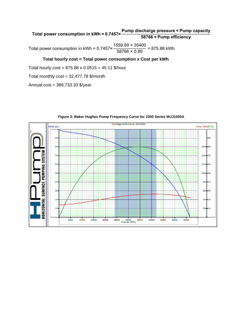
Total power consumption in kWh = 0.7457×Pump discharge pressure × Pump capacity

58766 × Pump efficiency

Total power consumption in kWh = 0.7457×1559.89 × 35400

58766 × 0.80 = 875.88 kWh

Total hourly cost = Total power consumption x Cost per kWh

Total hourly cost = 875.88 x 0.0515 = 45.11 $/hour

Total monthly cost = 32,477.78 $/month

Annual cost = 389,733.33 $/year

Figure 3: Baker Hughes Pump Frequency Curve for 1000 Series WJJ1000A

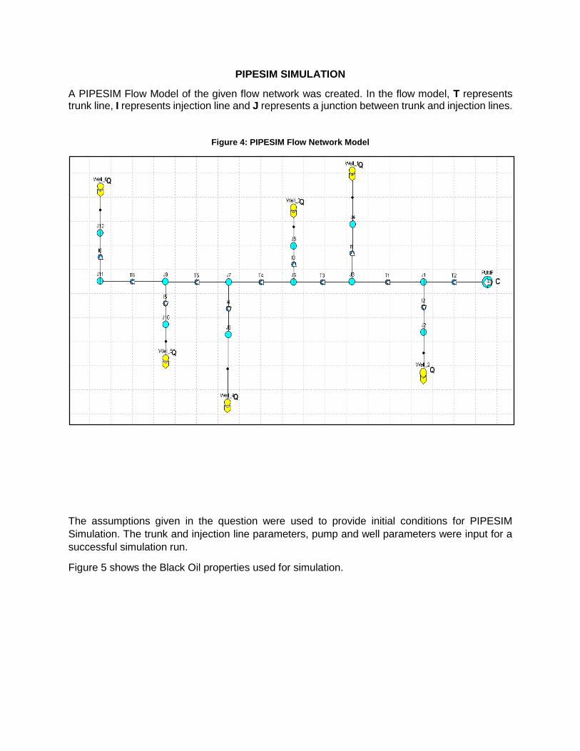
PIPESIM SIMULATION

A PIPESIM Flow Model of the given flow network was created. In the flow model, T represents trunk line, I represents injection line and J represents a junction between trunk and injection lines.

Figure 4: PIPESIM Flow Network Model

The assumptions given in the question were used to provide initial conditions for PIPESIM

Simulation. The trunk and injection line parameters, pump and well parameters were input for a

successful simulation run.

Figure 5 shows the Black Oil properties used for simulation.

Figure 5: Black Oil Properties

The simulation was run and the results so obtained were tabulated on Table 8.

Table 8: PIPESIM Simulation Run Results

No. Branch Name

Type Temperature,

degF Pressure, psia

Water Cut, %

Mass Flow Rate, lb/s

1 T_2 Trunk_Junction 60.017 1564.22 100 142.92

2 I_1 Injection_Junction 60.408 1406.27 100 23.27

3 I_2 Injection_Junction 60.093 1533.59 100 24.04

4 I_3 Injection_Junction 60.095 1533.11 100 24.34

5 I_4 Injection_Junction 60.175 1500.84 100 23.32

6 I_5 Injection_Junction 60.171 1502.35 100 24.03

7 I_6 Injection_Junction 60.203 1489.13 100 23.89

8 T_1 Trunk_Junction 60.041 1554.94 100 118.87

9 T_3 Trunk_Junction 60.078 1541.31 100 95.60

10 T_4 Trunk_Junction 60.079 1539.38 100 71.26

11 T_5 Trunk_Junction 60.085 1537.05 100 47.93

12 T_6 Trunk_Junction 60.099 1531.47 100 23.89

13 Well_1 Sink 60.4 1409.33 100 23.27

14 Well_2 Sink 60.092 1533.98 100 24.04

15 Well_3 Sink 60.094 1533.39 100 24.34

16 Well_4 Sink 60.173 1501.38 100 23.32

17 Well_5 Sink 60.181 1498.25 100 24.03

18 Well_6 Sink 60.218 1483.12 100 23.89

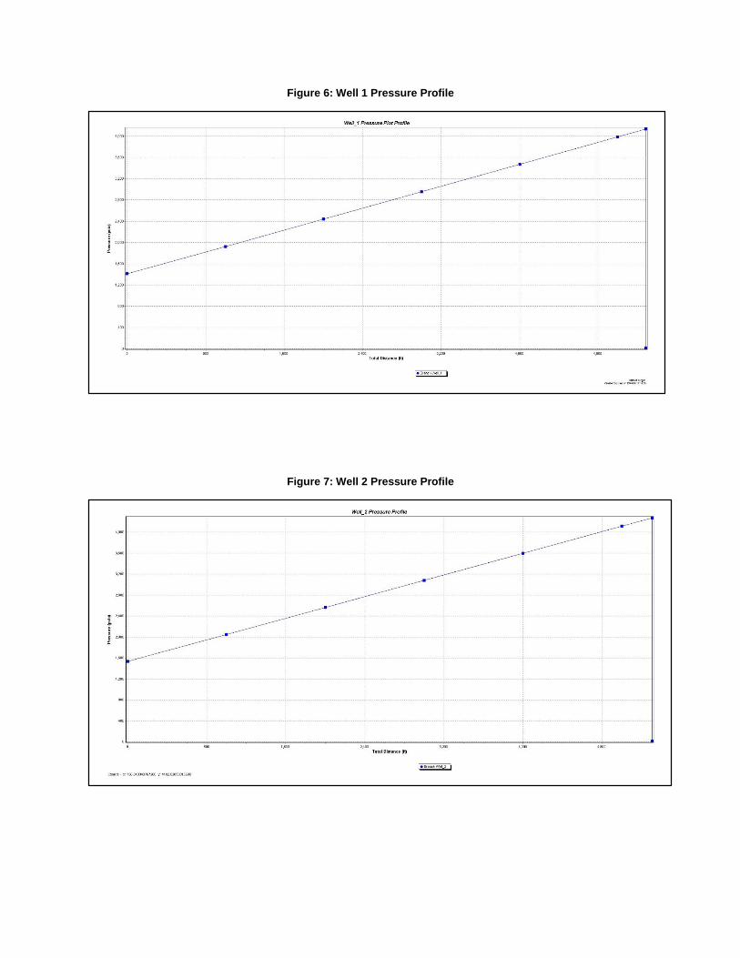
Figure 6: Well 1 Pressure Profile

Figure 7: Well 2 Pressure Profile

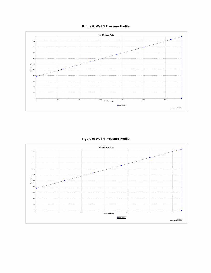
Figure 8: Well 3 Pressure Profile

Figure 9: Well 4 Pressure Profile

Figure 10: Well 5 Pressure Profile

Figure 11: Well 6 Pressure Profile

CONCLUSION

The calculated values and PIPESIM Model run values were compared and displayed in Table 9.

Table 9: Comparison of Actual Injection Pressures

Well # Calculated Discharge

Pressure, psi

PIPESIM Generated Discharge Pressure,

psi Error, %

1 1322.09 1406.27 6.37

2 1499.96 1533.59 2.24

3 1509.58 1533.11 1.56

4 1462.62 1500.84 2.61

5 1468.54 1502.35 2.30

6 1450.38 1489.13 2.67

On comparison of the calculated values and simulation generated values, we observe some

difference in the values. This difference may be due to the following reasons:

The temperature of fluid that flows through the pipeline may change due to friction. Thus,

the actual temperature in the pipeline may be more than our assumption of 60 degF.

Since the software employs a numerical approach to calculations, the results may be more

accurate, as compared to the analytical approach employed in MS Excel calculations.

Factors such as fluid velocity, friction factor and pipeline roughness may change during

fluid flow in the pipeline. This can also lead to calculation discrepancies.

Hand calculations are subjected to human error, which may not be the case for the values

generated by the PIPESIM software.