XM‐1100), which measures absorbance of each sample between
1,100 and 2,498 nm with 2‐nm increments. The NIR measures were
repeated for each sample and averaged.
2.7 | Statistical analyses
2.7.1 | Modelling NIR spectra to Leptocybe scores
We developed a programmable analysis pipeline in R (R Core Team,
2016) to process NIR spectral data and to fit chemometric models.
The process of building NIR models involves the use of mathematical
pretreatments (transformations) applied to the NIR spectra. The objec-
tive of applying those transformations is to remove the scattering of
diffuse reflections associated with sample particle size from the spec-
tra to improve the subsequent regression. The most widely used trans-
formation techniques can be divided into two categories: (a) scatter
correction methods and (b) spectral derivatives (Rinnan, van den Berg,
& Engelsen, 2009). In this study, we corrected the spectra using mul-
tiplicative scatter correction, standard normal variate and detrend
from the scatter correction methods; and a second derivative of
Savitzky–Golay smoothing with two different window sizes of 5 and
7 points from the spectral derivatives methods. Additionally, we com-
bined transformations by pairs applying scattering correction methods
prior to differentiation. Preprocessing of our NIR spectral data was
done using the R packages “ChemometricsWithR” (Wehrens, 2011)
and “Prospectr” (Stevens & Ramirez‐Lopez, 2013), we generated as
outcome a total of 12 data sets of predictor variables including the
raw spectra (Table S2A).
Local outliers factors were calculated for all observations on each
spectral database and used to identify outliers based on density and
distance (Breunig, Kriegel, Ng, & Sander, 2000). Individuals with local
outliers factors values greater than 2 were excluded from the analysis,
using a local outliers factors algorithm implemented in the R package
“DMwR” (Torgo, 2015). The percentage of individuals classified as
outliers for each set of models is given in Table S2B. Transformed
and outlier free databases were used to develop the NIR prediction
models for LS1, LS2, and IBV. For this purpose, we used partial least
squares implemented in the R‐package “pls” (Mevik & Wehrens,
2007). Two modelling scenarios were contemplated: first, we grouped
the observations by site and fitted models for each site, and second,
we used individual NIR spectra to fit models across all sites. For all
scenarios, we evaluated the performance of our models using leave‐
one‐out cross‐validation. Desirable partial least squares NIR models
are the ones that (a) maximize the coefficient of determination (R2),
(b) maximize the percentage of the variance explained for X and Y
on the training population (ExpVar_Y and ExpVar_X), (c) minimize the
standard errors of cross‐validation: root mean squared error of predic-
tion (RMSEP), and (d) have a small number of latent variables (projec-
tion factors).
2.7.2 | Modelling terpenes to Leptocybe scores
Bayesian model selection (Raftery, 1995) was performed in R, using
the “bicreg” function in the Bayesian model averaging (BMA) package
(Raftery, Hoeting, Volinsky, Painter, & Yeung, 2017), to identify which
of the 48 measured terpenes (predictor variables) were the most
important for predicting L. invasa infestation (Table S3A). We also con-
sidered the sums of certain groups of terpenes as possible predictor
variables (Table S3B). Terpenes were combined as a result of biological
motivation or high pairwise correlations (r > .6). Biological motivation
was based on either (a) shared intermediate carbocation (biosyntheti-
cally related through same intermediate precursor) or (b) the fact that
terpene X is a precursor of terpene Y (biosynthetically related by
“descent”); see Keszei, Brubaker, and Foley (2008) Figure 3a.
Instead of using stepwise variable selection to choose candidate
covariates, BMA accounts for uncertainty in variable selection by
averaging over the best models. The Bayesian information criterion
was used as a criterion for model selection and to estimate the poste-
rior probability of a given model. Terpene variable selection was per-
formed for the three dependent variables, LS1, LS2, and IBV,
respectively, using the same two modelling scenarios mentioned
above (first, models were fit per site and, second, across all sites).
To test whether the BMA model parameters were consistent, we
performed leave‐one‐out cross‐validation: the BMA analysis was
repeated n times, with n the number of individuals in the sample.
For each of these different training data sets (in accordance with the
leave‐one‐out cross‐validation strategy; the data of a different individ-
ual were excluded per iteration), the model with the lowest Bayesian
information criterion was used to estimate model coefficients,
whereafter the L. invasa screening value of the excluded individual
was predicted using the estimated model coefficients. Finally, a
leave‐one‐out cross‐validation R2 value was calculated by correlating
the predicted with the observed L. invasa screening values.
2.7.3 | Modelling NIR spectra to terpene scores
We build terpene composition models for samples as a function of
their NIR spectrum, following the same steps described above (trans-
formation to the spectral data, outlier identification, and partial least
squares modelling). Terpene models were performed only at site
SQF (site at which we found the best models, see Table 1 and Table
S5) and for the subset of terpenes that we found were the most
important for predicting L. invasa infestation. We also considered the
same combinations of terpenes mentioned in the previous section
(Table S3B) for fitting partial least squares models.
3 | RESULTS
3.1 | Leptocybe invasa infestation
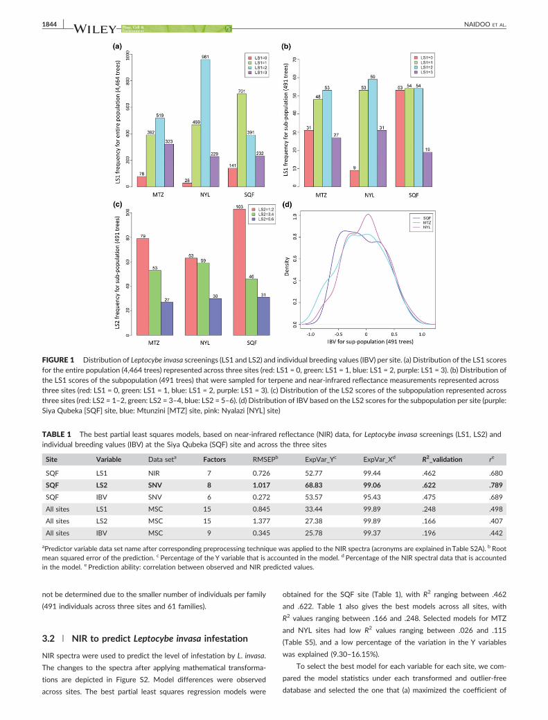
The distribution of LS1 across the three sites is indicated in Figure 1a.
The subpopulation was sampled for terpene and NIR measurements,
and the distribution of LS1, LS2, and IBV within this subpopulation is
shown in parts b, c, and d of Figure 1. The heritability values for the
E. grandis full population (126 families for LS1) and subpopulation
(61 families for LS2) at each site are indicated in Table S4. The type
B genetic correlations for LS1, for each pairwise combination of the
sites, were .71 (MTZ:NYL), .84 (MTZ:SQF), and .74 (SQF:NYL). The
type B genetic correlation for the three sites combined was .77, sug-
gesting that there was a relatively low level of G × E with little change
in family ranking between the sites. G × E for the subpopulation could
FIGURE 1 Distribution of Leptocybe invasa screenings (LS1 and LS2) and individual breeding values (IBV) per site. (a) Distribution of the LS1 scores
for the entire population (4,464 trees) represented across three sites (red: LS1 = 0, green: LS1 = 1, blue: LS1 = 2, purple: LS1 = 3). (b) Distribution ofthe LS1 scores of the subpopulation (491 trees) that were sampled for terpene and near‐infrared reflectance measurements represented acrossthree sites (red: LS1 = 0, green: LS1 = 1, blue: LS1 = 2, purple: LS1 = 3). (c) Distribution of the LS2 scores of the subpopulation represented acrossthree sites (red: LS2 = 1–2, green: LS2 = 3–4, blue: LS2 = 5–6). (d) Distribution of IBV based on the LS2 scores for the subpopulation per site (purple:Siya Qubeka [SQF] site, blue: Mtunzini [MTZ] site, pink: Nyalazi [NYL] site)
TABLE 1 The best partial least squares models, based on near‐infrared reflectance (NIR) data, for Leptocybe invasa screenings (LS1, LS2) andindividual breeding values (IBV) at the Siya Qubeka (SQF) site and across the three sites
Site Variable Data seta Factors RMSEPb ExpVar_Yc ExpVar_Xd R2_validation re
SQF LS1 NIR 7 0.726 52.77 99.44 .462 .680
SQF LS2 SNV 8 1.017 68.83 99.06 .622 .789
SQF IBV SNV 6 0.272 53.57 95.43 .475 .689
All sites LS1 MSC 15 0.845 33.44 99.89 .248 .498
All sites LS2 MSC 15 1.377 27.38 99.89 .166 .407
All sites IBV MSC 9 0.345 25.78 99.37 .196 .442
aPredictor variable data set name after corresponding preprocessing technique was applied to the NIR spectra (acronyms are explained inTable S2A). b Rootmean squared error of the prediction. c Percentage of the Y variable that is accounted in the model. d Percentage of the NIR spectral data that is accountedin the model. e Prediction ability: correlation between observed and NIR predicted values.
1844 NAIDOO ET AL.
not be determined due to the smaller number of individuals per family
(491 individuals across three sites and 61 families).
3.2 | NIR to predict Leptocybe invasa infestation
NIR spectra were used to predict the level of infestation by L. invasa.
The changes to the spectra after applying mathematical transforma-
tions are depicted in Figure S2. Model differences were observed
across sites. The best partial least squares regression models were
obtained for the SQF site (Table 1), with R2 ranging between .462
and .622. Table 1 also gives the best models across all sites, with
R2 values ranging between .166 and .248. Selected models for MTZ
and NYL sites had low R2 values ranging between .026 and .115
(Table S5), and a low percentage of the variation in the Y variables
was explained (9.30–16.15%).
To select the best model for each variable for each site, we com-
pared the model statistics under each transformed and outlier‐free
database and selected the one that (a) maximized the coefficient of
NAIDOO ET AL. 1845
determination (R2_validation), the prediction ability (r), and the per-
centage of the variance explained for X and Y on the training popu-
lation (ExpVar_Y and ExpVar_X), (b) minimize the standard errors
cross‐validation: RMSEP, and (c) have a small number of projection
factors. Table 2 shows all model statistics that were obtained for
each data set when modelling LS2 for the SQF site. For this case, a
standard normal variate transformed data set gives the best model.
Model diagnostic plots were also created for each data set and were
used to select the number of latent variables (factors) of each model.
Note that for LS2 under the standard normal variate data set (model
diagnostic plots in Figure 2), 8 factors give the highest R2 and the
lowest RMSEP. NIR models under the second scenario (across all
sites) did not perform well.
3.3 | Terpenes to predict Leptocybe invasainfestation
A descriptive analysis on the terpene measurements (48 terpenes) was
performed to explore the data. Figures S3A,B and S4, respectively,
show the hierarchical clustering dendrogram of the terpene measure-
ments across all sites, a graphical display of the all‐versus‐all terpene
correlation matrix, and a principal component analysis biplot
representing the relationship between the terpenes and the individual
trees grouped per site. From these analyses, it is evident that there are
groups of terpenes that are highly correlated, so we needed to find a
subset of terpenes to fit our models that minimize the likelihood of
TABLE 2 Partial least squares models, based on near‐infrared reflectanc
Data seta Factors RMSEPb ExpVar_Y
SNV 8 1.017 68.83
MSC 8 1.022 68.44
DT 5 1.075 62.68
SG5 5 1.079 67.33
SG7 5 1.073 65.94
SNV_SG5 5 1.084 68.02
SNV_SG7 5 1.077 66.55
MSC_SG5 5 1.085 68.01
MSC_SG7 5 1.078 66.54
DT_SG5 5 1.084 68.02
DT_SG7 5 1.077 66.55
NIR 5 1.120 60.33
aPredictor variable data set name after corresponding preprocessing technique wmean squared error of the prediction. c Percentage of the Y variable that is accoin the model. e Prediction ability: correlation between observed and NIR predic
FIGURE 2 Model diagnostics of Leptocybeinvasa screening 2 (LS2) with a standardnormal variate transformed database at theSiya Qubeka site. RMSEP = root meansquared error of the prediction
having multicollinearity problems. Figure S5A–C shows boxplots of
terpene concentration, separated by site.
The best BMA models were obtained for the SQF site (see Table
S6A–D for all BMA results). A summary of the most important terpenes
for predicting LS1, LS2, and IBV at the SQF site and across all sites,
together with the relevant model statistics, is presented in Table 3.
Seven terpenes from models at the SQF site were selected for further
analysis, that is, NIR modelling to predict terpene content. Figure 3
shows the hierarchical clustering dendrogram of the terpene measure-
ments at the SQF site, with the seven selected terpenes highlighted and
scattered across different clusters: T.2 (monoterpene 2), T.3 (α‐pinene),
(sesquiterpene 2), and T.46 (sesquiterpene 3). These terpenes were
the result of the top BMA model for both LS1 (R2 = .306) and LS2
(R2 = .346), and six of these terpenes were included in the model with
the highest R2 value (R2 = .302) for IBV (Table 3).
Performing leave‐one‐out cross‐validation on the BMA models at
the SQF site (and considering only the top Bayesian information crite-
rion‐ranked model per BMA run), four of the seven selected terpenes
were present in more than 90% of the models (monoterpene 2, α‐
pinene, γ‐terpinene, and sesquiterpene 3), and the remaining three
terpenes were added if the presence in more than 50% of the models
were considered (iso‐pinocarveol, sesquiterpene 1, and sesquiterpene
2). An additional three terpenes were added if the presence in more
than 35% of the models were considered (monoterpene 5, terpene
34, and terpene 37). The average number of factors (terpenes included
e (NIR) data, for Leptocybe invasa screening 2 at the Siya Qubeka site
c ExpVar_Xd R2_validation re
99.06 .622 .789
99.09 .619 .787
93.66 .577 .76
84.29 .574 .757
86.37 .578 .76
84.51 .569 .755
86.66 .575 .758
84.52 .569 .754
86.66 .574 .758
84.51 .569 .755
86.66 .575 .758
98.48 .540 .735
as applied to the NIR spectra (acronyms are explained inTable S2A). b Rootunted in the model. d Percentage of the NIR spectral data that is accountedted values.
TABLE 3 Bayesian model selection to identify the most important terpenes for predicting Leptocybe invasa infestation based on L. invasascreenings (LS1, LS2) and individual breeding values (IBV) at the Siya Qubeka (SQF) site and across all three sites. The model with the highest R2
value out of the top five Bayesian information criterion‐ranked models is reported
Cases where the indicated terpenes were not considered important for predicting L. invasa infestation.aTerpenes selected for near‐infrared reflectance modelling. bThe model number out of the top five Bayesian information criterion‐ranked models. cThenumber of variables selected for that model. d Leave‐one‐out (LOO) cross‐validation (CV) R2 value. eThe Bayesian information criterion (BIC) is a criterionfor model selection among a finite set of models. The model with the lowest BIC is preferred. fThe posterior probabilities of the models selected.
1846 NAIDOO ET AL.
in a model) across the cross‐validation models was 7 (min = 4 and
max = 7), and the average R2 was .34 (min = .27 and max = .36).
BMA models that were obtained across the top five LS1, LS2, and
IBV models from data of the MTZ site (average R2 = .129), the NYL
site (average R2 = .08), and across all sites (average R2 = .07) did not
perform well and were thus not considered in further analyses.
To further improve the BMAmodels for LS2 in the SQF site, differ-
ent combinations of predictor variables were included together with
individual terpenes as input to separate BMA analyses. Note that when
the sum of a group of monoterpenes was included, the separate mono-
terpenes (that made up the sum) were not included as predictor vari-
ables for that analysis. However, it was not possible to obtain a higher
R2 value than when the seven individual terpenes mentioned above
were included in the model (calibration R2 = .35 and validation R2 = .29).
3.4 | NIR to predict terpenes (SQF site)
Prediction models for terpene concentration were run for the seven
terpenes selected under BMA (see list of terpenes above). For those
terpenes, the best models were obtained for T.10 (iso‐pinocarveol),
T.3 (α‐pinene), and T.8 (γ‐terpinene) with R2 values ranging between
.188 and .333 and with prediction abilities between .433 and .577
(Table 4). Table 5 shows summary statistics of the best models obtained
when terpenes were combined based on either biological motivation or
high pairwise correlations (r > .6). Selection of best models was made
according to the following conditions: small number of latent variables
(factors) that minimize the RMSEP, maximize the proportion of varia-
tion explained for both the dependent and independent variables, and
maximize the cross‐validation R2. Prediction abilities of those models
ranged between .481 for sum(T3‐T5,T7,T10,T13‐T15) and .683 for
sum(T05,T07), the latter being the terpene combination for which we
obtained the best model with a 47% of the trait variation.
4 | DISCUSSION
We sought to associate terpene profiles with Leptocybe damage in a
subpopulation of an E. grandis breeding trial. There was phenotypic var-
iation of Leptocybe damage in the first year of L. invasa infestation
(Figure 1a) with the NYL site showing more Score 2 phenotypes (with
galls) and the SQF site showing more Score 0 phenotypes (absence of
galls). Within the subpopulation, the LS1 scores in NYL showed a higher
frequency of 3 and a lower frequency of 0 than the other two sites
(Figure 1b). In the second round of phenotyping after reinfestation by
L. invasa, all individuals showed the presence of galls (Score 1, Figure 1
c) with SQF appearing to contain more of the healthy phenotype (higher
frequency of Scores 1 and 2) compared with the other sites.
We detected 48 terpenes in the E. grandis individuals; however,
only a subset could be identified and were previously identified in
Eucalyptus species (Kainer et al., 2017; Padovan, Keszei, Wallis, &
Foley, 2012; Wallis et al., 2011). Eucalypts often contain distinct foliar
chemical variation within a species, termed “chemotypes,” where the
foliar chemical profile of one subpopulation is dominated by one or
FIGURE 3 Hierarchical clustering
dendrogram of the 48 measured terpenes atthe Siya Qubeka site. The seven terpenesselected for near‐infrared reflectancemodelling are boxed
NAIDOO ET AL. 1847
TABLE 4 The best partial least squares models, based on near‐infrared reflectance (NIR) data, to predict terpene content at the Siya Qubeka site
Variable Data seta Factors RMSEPb ExpVar_Yc ExpVar_Xd R2_validation re
aPredictor variable data set name after corresponding preprocessing technique was applied to the NIR spectra (acronyms are explained inTable S2A). b Rootmean squared error of the prediction. c Percentage of the Y variable that is accounted in the model. d Percentage of the NIR spectral data that is accountedin the model. e Prediction ability: correlation between observed and NIR predicted values.
1848 NAIDOO ET AL.
few chemicals, whereas another subpopulation is dominated by differ-
ent chemicals (Keszei et al., 2008; Padovan et al., 2014). Ecologically,
this type of variation is important as some pest or herbivores prefer-
entially eat only one chemotype (Moore et al., 2014; Padovan, Keszei,
Köllner, Degenhardt, & Foley, 2010). Although there has been no pre-
vious record of chemotypic variation in E. grandis, two closely related
species, Eucalyptus pelita and E. urophylla, have two described mono-
terpene chemotypes each, which are dominated by 1,8‐cineole and
α‐pinene and 1,8‐cineole and p‐cymene, respectively (Padovan et al.,
2014). We tested whether this progeny trial contained distinct
chemotypes but could not identify any. The terpene profile of every
individual was dominated by α‐pinene. Previous attempts to identify
chemotypic variation in E. grandis did not test many individuals
(Brophy & Southwell, 2002), which prompted us to test for such vari-
ation in a larger population; however, due to some degree of intro-
gression due to the ongoing inbreeding programme of E. grandis in
South Africa, the potential full chemical variation of this species has
still not been elucidated.
Using the phenotypes captured for the 491 E. grandis individuals
over two infestation seasons, we successfully developed models to
predict L. invasa infestation scores based on NIR spectra (Tables 1
and 2) and terpene content (Table 3). We also related NIR to ter-
penes (Tables 4 and 5). The selected models, indicated in bold text
in Tables 2, 3, and 5, explain 62%, 29%, and 47% of the trait varia-
tion, respectively. The performance of models was evaluated using
leave‐one‐out cross‐validation. In general, models with RMSEP
values smaller than .3 indicate very good predictive models
(Veerasamy et al., 2011).
TABLE 5 The best partial least squares models, based on near‐infrared reQubeka site
Variable Data seta Factors RMSEP
sum(T10,T14)f SG7 9 0.207
sum(T5,T7)f SG7 13 1.181
sum(T7,T15)g SG7 12 1.154
sum(T6,T8)g DT_SG7 12 1.249
sum(T5,T7,T15)g SG7 12 1.249
sum(T3‐T5,T7, T10,T13‐T15)g SG7 8 2.958
aPredictor variable data set name after corresponding preprocessing technique wmean squared error of the prediction. c Percentage of the Y variable that is accoin the model. e Prediction ability: correlation between observed and NIR predictegReason for combining terpenes: biological motivation; based on (a) shared inteprecursor) or (b) terpene X is precursor of terpene Y (biosynthetically related b
There was a marked discrepancy in site for models that explained
the NIR and terpene association with L. invasa scores. In both cases,
that is, using NIR and terpene data, the only site that passed our
criteria of acceptable models was SQF. This is in agreement with our
calculations of heritability for LS2 per site. For MTZ and NYL, we
found negligible heritability values, so the variation of the L. invasa
score is mainly due to environmental conditions or random experi-
mental variation. In contrast, SQF had a heritability value of 0.16,
being the only test in which genetic variation was found between indi-
viduals (Table S4) contributing to better models. G × E could not be
determined for the 491 individuals, but a low G × E was estimated
for the full E. grandis population. Table S1 indicates that there were
some slight differences in the environmental data for the three sites.
SQF and MTZ had higher moisture content than NYL. The MTZ site
contains a hardy grass, which is thought to compete with E. grandis
growth during establishment. The percentage stocking at 4‐year was
88% for SQF, 81% for NYL, and 67% for MTZ. The average diameter
at breast height was highest at site SQF (Table S1). Collectively, this
suggests that SQF has the best growth conditions out of the sites
sampled. Interestingly, SQF had a higher proportion of Scores 0 and
1 for LS1 and Scores 1 and 2 for LS2 than the other two sites—indicat-
ing a more resistant phenotype (Figure 1a,c).
When modelling terpene effects on L. invasa score, we found that
the terpenes that most contributed to the models act in opposing direc-
tions (seeTable S3C and coefficients in Table S6A). One group, includ-
ing α‐pinene, γ‐terpinene, and sesquiterpene 1, showed increasing
damage to trees with increasing concentration of terpenes. α‐Pinene
has a relatively high vapour pressure (3 mmHg at 20 °C) compared with
flectance (NIR) data, to predict monoterpene combinations for the Siya
b ExpVar_Yc ExpVar_Xd R2_validation re
59.55 94.39 .349 .591
82.90 96.96 .466 .683
78.94 96.75 .461 .679
72.41 96.67 .335 .579
78.57 96.75 .454 .674
50.97 93.15 .231 .481
as applied to the NIR spectra (acronyms are explained inTable S2A). b Rootunted in the model. d Percentage of the NIR spectral data that is accountedd values. fReason for combining terpenes: high pair‐wise correlation (r > .6).rmediate carbocation (biosynthetically related through same intermediatey “descent”). This is based on Keszei et al. (2008) Figure 3a.
NAIDOO ET AL. 1849
other monoterpenes and is therefore more volatile than most monoter-
penes commonly found in eucalypts. Ladybeetles are attracted to α‐
pinene from persimmon (Diospyros kaki; Zhang, Xie, Xue, Peng, &Wang,
2009), whereas trap catch of the invasive pine bark beetle Hylurgus
ligniperda was increased to over 200‐fold when α‐pinene was used as
an attractant (Kerr, Kelly, Bader, & Brockerhoff, 2017); therefore, we
could expect α‐pinene to act as a volatile cue for L. invasa oviposition.
γ‐Terpinene levels were constitutively higher in the susceptible clone
GC540 compared with the resistant E. grandis clone TAG5 and were
induced to much higher levels upon insect oviposition (Oates et al.,
2015). Interestingly, the levels of γ‐terpinene decreased in the resistant
genotype after infestation (Oates et al., 2015). It is feasible that γ‐
terpinene may play a role in promoting susceptibility to the insect pest;
however, this remains to be demonstrated.
The other group of terpenes (including monoterpene 2, iso‐
pinocarveol, sesquiterpene 2, and sesquiterpene 3) acting in the oppo-
site direction may play a direct role in defence against L. invasa, where
higher concentrations of the compound lead to reduced damage by
L. invasa. Evidence from other systems indicates that this could be
achieved through different ways, such as direct toxic effect on larvae
leading to either death or reduced growth of larvae (McLean et al.,
1993), or through indirect defences by attracting parasites through
tritrophic ways (reviewed in Gershenzon & Dudareva, 2007). Several
parasitoids of L. invasa have been identified with some being
adopted for biological control (e.g., Seletrichoides neseri, Ophelimus
maskelli, and Seletrichoides kyceri; reviewed in Zheng et al., 2014);
however, the volatile cues that attract these parasitic wasps have
not been investigated. In a study by Visser, Wegrzyn, Steenkmap,
Myburg, and Naidoo (2015), artificial inoculation of the E. grandis
clone TAG5 with the fungal pathogen Chrysoporthe austroafricana
led to the induction of iso‐pinocarveol systemically, in leaf tissue.
This E. grandis clone was also found to be resistant to L. invasa
(Oates et al., 2015).
In summary, we produced models for terpene to L. invasa infes-
tation, NIR to terpenes, and NIR to L. invasa interactions in E. grandis
that explained 29% (Table 3, bold text), 47% (Table 5, bold text), and
62% (Table 2, bold text) of the trait variation, respectively. These
methods developed in this study can be utilized as a guideline to
model other plant–insect interaction systems as NIR may be a more
cost‐effective approach to modelling resistance. One approach to
improve the model would involve setting up a similar experiment
in a controlled environment where the best and the worst
performing individuals were cloned and exposed to L. invasa so that
robust phenotypes may be observed. In this manner, stronger asso-
ciations could be derived for terpenes and resistance to L. invasa
revealing important cues that could act as attractants and repellents
against the insect pest.
ACKNOWLEDGMENTS
The authors acknowledge funding from the National Research Foun-
dation (NRF) South Africa Bioinformatics and Functional Genomics
Programme (Grant ID 89669) and the Department of Science and
Technology Eucalyptus genomics platform grant. We thank Ms Jessie
Au and Dr Amanda Padovan for assistance with the leaf sample prep-
Alves, M. D. C. S., Filho, S. M., Innecco, R., & Torres, S. B. (2004). Alelopatiade extratos voláteis na germinação de sementes e no comprimento daraiz de alface. Pesquisa Agropecuária Brasileira, 39, 1083–1086.
Breunig, M. M., Kriegel, H.‐P., Ng, R. T., & Sander, J. (2000). LOF: Identify-ing density‐based local outliers. ACM SIGMOD Record, 29, 93–104.
Brophy, J. J., & Southwell, I. A. (2002). Eucalyptus chemistry. In J. J. W.Coppen (Ed.), Eucalyptus—The genus Eucalyptus (pp. 102–160). London:Taylor and Francis.
Burdon, R. D. (1977). Genetic correlation as a concept for studying geno-type‐environment interaction in forest tree breeding. Silvae Genetics,26, 168–175.
Carr, D. J., & Carr, S. G. M. (1970). Oil glands and ducts in EucalyptusL'Herit. II: Development and structure of oil glands in the embryo. Aus-tralian Journal of Botany, 18, 191–212.
Chang, R., Arnold, R., & Zhou, X. (2012). Association between enzymeactivity levels in Eucalyptus clones and their susceptibility to the gallwasp, Leptocybe Invasa, in South China. Journal of Tropical Forest Sci-ence, 24, 256–264.
Coppen, J. J. W. (2003). Eucalyptus: The genus Eucalyptus. London: CRCPress LLC.
De Moraes, C. M., Lewis, W. J., Paré, P. W., Alborn, H. T., & Tumlinson, J. H.(1998). Herbivore‐infested plants selectively attract parasitoids. Nature,393, 570–573.
Degenhardt, J., & Gershenzon, J. (2003). Terpenoids. In T. Brian, D. Mur-phy, & B. Murray (Eds.), Encyclopedia of applied plant sciences (pp.500–504). Amsterdam: Elsevier.
Dittrich‐Schröder, G., Harney, M., Neser, S., Joffe, T., Bush, S., Hurley, B. P.,… Slippers, B. (2014). Biology and host preference of Selitrichodesneseri: A potential biological control agent of the Eucalyptus gall wasp,Leptocybe invasa. Biological Control, 78, 33–41.
Dittrich‐Schröder, G., Wingfield, M. J., Hurley, B. P., & Slippers, B. (2012).Diversity in Eucalyptus susceptibility to the gall forming wasp L. invasa.Agricultural and Forest Entomology, 14, 419–427.
Dudareva, N., Andersson, S., Orlova, I., Gatto, N., Reichelt, M., Rhodes, D.,… Gershenzon, J. (2005). The nonmevalonate pathway supports bothmonoterpene and sesquiterpene formation in snapdragon flowers. Pro-ceedings of the National Academy of Sciences, 102, 933–938.
Durand, N., Rodrigues, J. C., Mateus, E., Boavida, C., & Branco, M. (2011).Susceptibility variation in Eucalyptus spp in relation to Leptocybe invasaand Ophelimus maskelli, two invasive gall wasps occurring in Portugal.Silva Lusitana, 19–31.
Edwards, P. B., Wanjura, W. J., & Brown, W. V. (1993). Selective herbivoryby Christmas beetles in response to intraspecific variation in Eucalyptusterpenoids. Oecologia, 95, 551–557.
Edwards, P. B., Wanjura, W. J., Brown, W. V., & Dearn, J. M. (1990). Mosaicresistance in plants. Nature, 347, 434.
Eyles, A., Davies, N. W., Yuan, Z. Q., & Mohammed, C. (2003). Hostresponses to natural infection by Cytonaema sp. in the aerial bark ofEucalyptus globulus. Forest Pathology, 33, 317–331.
Gershenzon, J., & Dudareva, N. (2007). The function of terpene naturalproducts in the natural world. Nature Chemical Biology, 3, 408–414.
Giamakis, A., Kretsi, O., Chinou, I., & Spyropoulos, C. G. (2001). Eucalyp-tus camaldulensis: Volatiles from immature flowers and highproduction of 1,8‐cineole and β‐pinene by in vitro cultures. Phyto-chemistry, 58, 351–355.
Gomes, V. J., Longue, D., Colodette, J. L., & Ribeiro, R. A. (2014). The effectof eucalypt pulp xylan content on its bleachability, refinability anddrainability. Cellulose, 21, 607–614.
Henery, M. L., Wallis, I. R., Stone, C., & Foley, W. J. (2008). Methyljasmonate does not induce changes in Eucalyptus grandis leaves thatalter the effect of constitutive defences on larvae of a specialist herbi-vore. Oecologia, 156, 847–859.
Iqbal, Z., Akhtar, M., Qureshi, T. M., Akhter, J., & Ahmad, R. (2011). Varia-tion in composition and yield of foliage oil of Eucalyptus polybractea.Journal of the Chemical Society of Pakistan, 33, 183–187.
Javaregowda, J., & Prabhu, S. T. (2010). Susceptibility of eucalyptus speciesand clones to gall wasp, Leptocybe invasa Fisher and La Salle(Eulophidae: Hymenoptera) in Karnataka. Karnataka Journal of Agricul-tural Science, 23, 220–221.
Kainer, D., Bush, D., Foley, W. J., & Külheim, C. (2017). Assessment of anon‐destructive method to predict oil yield in Eucalyptus polybractea(blue mallee). Industrial Crops and Products, 102, 32–44.
Keefover‐Ring, K., Thompson, J. D., & Linhart, Y. B. (2009). Beyond sixscents: Defining a seventh Thymus vulgaris chemotype new tosouthern France by ethanol extraction. Flavour and Fragrance Journal,24, 117–122.
Kelly, J., La Salle, J., Harney, M., Dittrich‐Schroder, G., Hurley, B. P., &Undefined, O. (2012). Selitrichodes neseri n. sp, a new parasitoid ofthe eucalyptus gall wasp Leptocybe invasa Fisher & La Salle (Hymenop-tera: Eulophidae: Tetrastichinae). Zootaxa, 3333, 50–57.
Kerr, J. L., Kelly, D., Bader, M. K. F., & Brockerhoff, E. G. (2017). Olfactorycues, visual cues, and semiochemical diversity interact during host loca-tion by invasive forest beetles. Journal of Chemical Ecology, 43, 17–25.
Keszei, A., Brubaker, C. L., & Foley, W. J. (2008). A molecular perspectiveon terpene variation in Australian Myrtaceae. Australian Journal of Bot-any, 56, 197–213.
Kim, I. K., Mendel, Z., Protasov, A., Blumberg, D., & La Salle, J. (2008). Tax-onomy, biology, and efficacy of two Australian parasitoids of theeucalyptus gall wasp, Leptocybe invasa Fisher & La Salle (Hymenoptera:Eulophidae: Tetrastichinae). Zootaxa, 1910, 1–20.
Külheim, C., Padovan, A., Hefer, C., Krause, S. T., Köllner, T. G., Myburg, A.A., … Foley, W. J. (2015). The Eucalyptus terpene synthase gene family.BMC Genomics, 16, 450.
Kulkarni, H. (2010). Screening eucalyptus clones against Leptocybe invasaFisher and La Salle (Hymenoptera: Eulophidae). Karnataka Journal ofAgricultural Science, 23, 87–90.
Lawler, I. R., Stapley, J., Foley, W. J., & Eschler, B. M. (1999). Ecologicalexample of conditioned flavor aversion in plant‐herbivore interactions:Effect of terpenes of Eucalyptus leaves on feeding by common ringtailand brushtail possums. Journal of Chemical Ecology, 25, 401–415.
McLean, S., Foley, W. J., Davies, N. W., Brandon, S., Duo, L., & Blackman,A. J. (1993). Metabolic fate of dietary terpenes from Eucalyptus radiatain common ringtail possum (Pseudocheirus peregrinus). Journal of Chem-ical Ecology, 19, 1625–1643.
Mendel, Z., Protasov, A., Fisher, N., & La Salle, J. (2004). Taxonomy andbiology of Leptocybe invasa gen. & sp. n. (Hymenoptera: Eulophidae),an invasive gall inducer on Eucalyptus. Australian Journal of Entomology,43, 101–113.
Mevik, B.‐H., & Wehrens, R. (2007). The pls package: Principal componentand partial least squares regression in R. Journal of Statistical Software,18, 1–23.
Mewalal, R., Rai, D. K., Kainer, D., Chen, F., Külheim, C., Peter, G. F., &Tuskan, G. A. (2017). Plant‐derived terpenes: A feedstock for specialtybiofuels. Trends in Biotechnology, 35, 227–240.
Moore, B., Andrew, R., Külheim, C., & Foley, W. (2014). Explaining intra-specific diversity in plant secondary metabolites in an ecologicalcontext. The New Phytologist, 201, 733–750.
Morrow, P. A., & Fox, L. R. (1980). Effects of variation in Eucalyptusessential oil yield on insect growth and grazing damage. Oecologia,45, 209–219.
Mutitu, K. E. (2003). A pest threat to Eucalyptus species in Kenya. KEFRITechnology Reports, 12.
Nyeko, P. (2005). The cause, incidence and severity of a new gall damageon Eucalyptus species at Oruchinga refugee settlement in Mbarara dis-trict, Uganda. Uganda Journal of Agricultural Science, 11, 47–50.
Nyeko, P., Mutitu, E. K., & Day, R. K. (2009). Eucalyptus infestation byLeptocybe invasa in Uganda. African Journal of Ecology, 47, 299–307.
Nyeko, P., & Nakabonge, G. (2008). Occurence of pests and diseases intree nurseries and plantations in Uganda. Sawlog Production GrantScheme, Kampala, Uganda.
Oates, C. N., Külheim, C., Myburg, A. A., Slippers, B., & Naidoo, S. (2015).The transcriptome and terpene profile of Eucalyptus grandis revealsmechanisms of defense against the insect pest, Leptocybe invasa. Plant& Cell Physiology, 56, 1418–1428.
Padovan, A., Keszei, A., Köllner, T. G., Degenhardt, J., & Foley, W. J.(2010). The molecular basis of host plant selection in Melaleucaquinquenervia by a successful biological control agent. Phytochemistry,71, 1237–1244.
Padovan, A., Keszei, A., Külheim, C., & Foley, W. J. (2014). The evolutionof foliar terpene diversity in Myrtaceae. Phytochemistry Reviews, 13,695–716.
Padovan, A., Keszei, A., Wallis, I. R., & Foley, W. J. (2012). Mosaic Eucalypttrees suggest genetic control at a point that influences several meta-bolic pathways. Journal of Chemical Ecology, 38, 914–923.
Padovan, A., Webb, H., Mazanec, R., Grayling, P., Bartle, J., Foley, W. J., &Külheim, C. (2017). Association genetics of essential oil traits in Euca-lyptus loxophleba: Explaining variation in oil yield. Molecular Breeding,37, 73.
Pateraki, I., Heskes, A., & Hamberger, B. (2015). Cytochromes P450 for ter-pene functionalization and metabolic engineering. In J. Schrader, & J.Bohlmann (Eds.), Biotechnology of isoprenoids (pp. 107–139). Cham:Springer International Publishing.
Quang Thu, P., Dell, B., & Isobel Burgess, T. (2009). Susceptibility of 18eucalypt species to the gall wasp Leptocybe invasa in the nursery andyoung plantations in Vietnam. ScienceAsia, 35, 113–117.
R CoreTeam (2016). R: A language and environment for statistical computing.Vienna, Austria: R Foundation for Statistical Computing. Retrievedfrom https://www.R‐project.org/
Raftery, A. A., Hoeting, J., Volinsky, C., Painter, I., & Yeung, K. Y. (2017).Bayesian model averaging. Retrieved from https://cran.r‐project.org/web/packages/BMA/BMA.pdf
Raftery, A. E. (1995). Bayesian model selection in social research. Sociolog-ical Methodology, 25, 111–163.
Rinnan, Å., van den Berg, F., & Engelsen, S. B. (2009). Review of the mostcommon pre‐processing techniques for near‐infrared spectra. Trends inAnalytical Chemistry, 28, 1201–1222.
Rivas, F., Parra, A., Martinez, A., & Garcia‐Granados, A. (2013). Enzymaticglycosylation of terpenoids. Phytochemistry Reviews, 12, 327–339.
Schimleck, L. R., & Rimbawanto, A. (2003). Near infrared spectroscopy forcost effective screening of foliar oil characteristics in a Melaleucacajuputi breeding population. Journal of Agricultural and Food Chemistry,51, 2433–2437.
Schnee, C., Kollner, T. G., Gershenzon, J., & Degenhardt, J. (2002). Themaize gene terpene synthase 1 encodes a sesquiterpene synthase cata-lyzing the formation of (E)‐β‐farnesene, (E)‐nerolidol, and (E,E)‐farnesolafter herbivore damage. Plant Physiology, 130, 2049–2060.
Squillace, A. E. (1974). Average genetic correlations among offspring fromopen‐pollinated forest trees. Silvae Genetics, 23, 149–156.
Stevens, A., & Ramirez‐Lopez, L. (2013). An introduction to the prospectrpackage. R package Vignette R package version 0.1.3. Retrieved fromhttps://cran.r‐project.org/web/packages/prospectr/vignettes/prospectr‐intro.pdf
Stone, C., & Bacon, P. E. (1994). Relationships among moisture stress,insect herbivory, foliar cineole content and the growth of river redgum Eucalyptus camaldulensis. Journal of Applied Ecology, 31, 604–612.
Torgo, L. (2015). Functions and data for “Data Mining with R”. Retrievedfrom https://cran.r‐project.org/web/packages/DMwR/DMwR.pdf
Turlings, T. C., Loughrin, J. H., McCall, P. J., Rose, U. S., Lewis, W. J., &Tumlinson, J. H. (1995). How caterpillar‐damaged plants protect them-selves by attracting parasitic wasps. Proceedings of the NationalAcademy of Sciences, 92, 4169–4174.
Veerasamy, R., Rajak, H., Jain, A., Sivadasan, S., Varghese, C. P., & Agrawal,R. K. (2011). Validation of QSAR models‐strategies and importance.International Journal of Drug Design & Disocovery, 2, 511–519.
Visser, E. A., Wegrzyn, J. L., Steenkmap, E. T., Myburg, A. A., & Naidoo, S.(2015). Combined de novo and genome guided assembly and annotationof the Pinus patula juvenile shoot transcriptome. BMCGenomics, 16, 1057.
Wallis, I. R., Keszei, A., Henery, M. L., Moran, G. F., Forrester, R., Maintz, J.,… Foley, W. J. (2011). A chemical perspective on the evolution of var-iation in Eucalyptus globulus. Perspectives in Plant Ecology, Evolution andSystematics, 13, 305–318.
Webb, H., Foley, W. J., & Külheim, C. (2014). The genetic basis of foliar ter-pene yield: Implications for breeding and profitability of Australianessential oil crops. Plant Biotechnology, 31, 363–376.
Wehrens, R. (2011). Chemometrics with R—Multivariate data analysis in thenatural sciences and life sciences Retrieved from https://cran.r‐project.org/web/packages/ChemometricsWithR/ChemometricsWithR.pdf
Wiley, J., & Skelley, P. (2008). A Eucalyptus pest, Leptocybe invasa Fisherand LaSalle (Hymenoptera: Eulophidae), genus and species new to Flor-ida and North America. Florida Department of Agriculture and ConsumerServices, 38870–38871.
Wilson, N. D., Watt, R. A., & Moffat, A. C. (2001). A near‐infrared methodfor the assay of cineole in eucalyptus oil as an alternative to the officialBP method. The Journal of Pharmacy and Pharmacology, 53, 95–102.
Wingfield, M., Slippers, B., Hurley, B., Coutinho, T., Wingfield, B., & Roux, J.(2008). Eucalypt pests and diseases: Growing threats to plantation pro-ductivity. South African Journal of Science, 70, 139–144.
Wong, Y. F., Perlmutter, P., & Marriott, P. J. (2017). Untargeted metabolicprofiling of Eucalyptus spp. leaf oils using comprehensive two‐dimen-sional gas chromatography with high resolution mass spectrometry:Expanding the metabolic coverage. Metabolomics, 13, 46.
Wylie, F., & Speight, R. (2012). Insect pests in tropical forestry. Wallingford,UK: CABI Publishing.
Zhang, Y., Xie, Y., Xue, J., Peng, G., & Wang, X. (2009). Effect of volatileemissions, especially α‐pinene, from persimmon trees infested by Jap-anese wax scales or treated with methyl jasmonate on recruitment ofladybeetle predators. Environmental Entomology, 38, 1439–1445.
Zheng, X. L., Li, J., Yang, Z. D., Xian, Z. H., Wei, J. G., Lei, C. L., … Lu, W.(2014). A review of invasive biology, prevalence and management ofLeptocybe invasa Fisher & La Salle (Hymenoptera: Eulophidae:Tetrastichinae). African Entomology: Journal of the Entomological Societyof Southern Africa, 22, 68–79.
Zhu, F. l., Ren, S., Qiu, B., Huang, Z., & Peng, Z. (2012). The abundance andpopulation dynamics of Leptocybe invasa (Hymenoptera: Eulophidae)galls on Eucalyptus spp. in China. Journal of Integrative Agriculture, 11,2116–2123.
SUPPORTING INFORMATION
Additional supporting information may be found online in the
Supporting Information section at the end of the article.
How to cite this article: Naidoo S, Christie N, Acosta JJ, et al.
Terpenes associated with resistance against the gall wasp,
Leptocybe invasa, in Eucalyptus grandis. Plant Cell Environ.