Sofia University "St. Kliment Ohridski" Faculty of Physics Department Meteorology and Geophysics Terrestrial water storage anomaly during the 2007 heat wave in Bulgaria Master Thesis of Biliana Rumenova Mircheva f.n. 180073 Thesis supervisor: /Assoc. prof. G. Guerova/ Head of Department: /Assoc. prof. N. Rachev/ Reviewer: /Head assist. prof. M. Tsekov/ Sofia April 2016
Transcript
Sofia University "St. Kliment Ohridski"Faculty of Physics
Department Meteorology and Geophysics
Terrestrial water storage anomalyduring the 2007 heat wave in
3.1 (a) Temperature time series for period 2003-2013; (b) movingaverage of length 6; (c) monthly mean temperatures for 2003-2013 (dashed line) and for 2007 (thick line); (d) anomalies for2007 versus 2003-2013. . . . . . . . . . . . . . . . . . . . . . . . 25
3.2 (a) Precipitation time series for period 2003-2013; (b) movingaverage of length 6; (c) monthly mean precipitation for 2003-2013 (dashed line) and for 2007 (thick line); (d) precipitationanomalies for 2007 versus 2003-2013. . . . . . . . . . . . . . . . 26
3.3 (a) IWV time series for period 2003-2013; (b) moving averageof length 6; (c) monthly mean IWV for 2003-2013 (dashed line)and for 2007 (thick line); (d) IWV anomalies for 2007 versus2003-2013. . . . . . . . . . . . . . . . . . . . . . . . . . . . . . 27
3.4 (a) TWS variations time series for period 2003-2013 with smooth-ing radii of 300 km (R1 - black line), 500 km (R2 - red line) and700 km (R3 - blue line); (b) moving average of length 6; (c)monthly mean TWS changes for 2003-2013 (dashed line) andfor 2007 (thick line); (d) TWS anomalies for 2007 versus 2003-2013. . . . . . . . . . . . . . . . . . . . . . . . . . . . . . . . . 28
4.1 Temperature (top) and precipitation anomalies (bottom) for2007 from SYNOP observations (black circles) and ALADIN-Climate model (red circles). . . . . . . . . . . . . . . . . . . . . 33
4.2 IWV anomaly for 2007 from GNSS observations (black circles)and ALADIN-Climate model (red circles). . . . . . . . . . . . . 34
4.3 TWS anomaly for 2007 from GRACE observations (black cir-cles) and ALADIN-Climate model (red circles). . . . . . . . . . 34
List of Tables
2.1 Coordinates of observation and model grid point. . . . . . . . . 20
4.1 Correlation coefficient of 2007 anomalies of temperature (T),precipitation (PP), IWV and TWS. . . . . . . . . . . . . . . . . 31
4.2 Observation and model anomalies for 2007 versus 2003-2008. . . 31
4
5
Abstract
Heat waves have large adverse social, economic and environmental effects in-cluding increased mortality, transport restrictions and a decreased agriculturalproduction. The estimated economic losses of the 2007 heat wave in SoutheastEurope exceed 2 billion EUR with 19 000 hospitalisation in Romania only. Theaim of this study is to investigate the anomalies of temperature, precipitation,integrated water vapour (IWV) and terrestrial water storage (TWS) in 2007compared to 2003-2013, that could have lead to the heat wave.
The heat wave month (July 2007) was 2◦ C hotter than the 2003-2013mean in Sofia, Bulgaria. The 2007 annual precipitation was on 10 % higherthan the 2003-2013 mean, but in spring the negative precipitation anomalyin April was followed by a large positive anomaly in May. A large negativeprecipitation anomaly is recorded in July 2007. In alignment with the precip-itation, IWV computed from a GNSS station in Sofia shows a large positiveanomaly in May 2007, while a negative anomaly in July. The terrestrial waterstorage anomaly, derived from the GRACE mission, has one month of delayand with a negative anomaly recorded in August 2007. It is possible that isdue to the slower soil response to the atmospheric drying and the heat.
Intercomparison is performed for the period 2003-2008 with ALADIN-Climate regional climate model. The following can be concluded for 2007anomalies in the model and observations: 1) a strong correlation for tem-perature and IWV anomalies data sets and 2) a weak relation between theprecipitation and TWS anomalies data set.
Chapter 1
Introduction
Climate change include variations in water and energy cycles on Earth. Ac-cording to Stocker et al. (2013) the global mean temperature increases yearafter year with 2015 being the hottest year in the records. Higher global tem-perature leads to changes in the hydrological cycle. For example increase oftemperature with 1◦ C leads to 7 % increase in water vapour, in agreement withthe Clausius-Clapeyron equation (Dai , 2006). Thus more water is evaporatedproviding appropriate conditions for intensive and powerful storms, reducingthe ground water content and increasing in the frequency of occurrence of ex-treme weather events in different parts of the world (Matzarakis et al., 2007).
Presented in figure 1.1 are the components of hydrology cycle: wa-ter vapour, liquid water, rain and water storage on earth surface and be-low. A complete description of the global water cycle is still a challenge. Atpresent, the hydrology cycle components like evaporation, cloud formation,evapo-transpiration, soil moisture content are studied in isolation and inte-grated in some way using computer models (Trenberth et al., 2006). Despitethe efforts, the global picture of the hydrology cycle and its changes is stillunclear. There is a lack of information due to the difficulties of collecting dataover oceans and other inaccessible terrains. There are uncertainties in quanti-ties of river run-off, stream flows, ice sheets and groundwater content. Routinemonitoring of hydrology components requires the collection and processing oflarge quantity of data.
6
Introduction 7
Figure 1.1: Water cycle components, image credit: web (b).
Essential component of the hydrology cycle is the Terrestrial WaterStorage (TWS) defined as all forms of water above and beneath the surface ofthe Earth. TWS is an aggregation of the amounts of ground water, soil mois-ture, surface water, snow, ice and vegetation water content. Thus TWS vari-ability is the sum of changes in snow, soil moisture, and ground water. TWSvaries in space and time. For understanding TWS major role in the climatesystem it is necessary to measure and analyse its spatio-temporal variations bydifferent methods. The TWS changes can be produced using combination ofadvanced land surface models for evaporation, precipitation and soil moisturecontent, reliable observations, and statistical assimilation techniques. Becauseof the complexity of TWS structure and components it is difficult to get a pre-cise global or regional description. In the past decades satellite missions werethe main source of data to study Earth’s hydrological components includingTWS.
One such missions is the Gravity Recovery And Climate Experiment(GRACE). GRACE is a polar orbiting twin satellite launched in 2002. GRACE
Introduction 8
Figure 1.2: Global TWS anomaly trend for 2003-2009, image credit: web (c).
maps changes in Earth’s gravity field, which can be converted to water massvariations and column-integrated TWS variations. The ability of obtaininginformation below the first several centimetres of the land surface is whatmakes GRACE so valuable for hydrological researches and applications suchas drought monitoring. The GRACE mission has been completed, but theGRACE Follow-On (GRACE-FO) mission will be deployed in 2017 (web, e)and will be used to continue the monitoring of gravity anomalies. With itsglobal coverage GRACE provides global maps of TWS anomalies. In figure1.2 are shown the significant changes in terrestrial water mass trends, on aglobal scale that occurred between 2003 and 2009. For example there are lossesin Alaskan and Himalayan glaciers, Greenland, Patagonia ice fields and WestAntarctica. Also there is depletion of groundwater in India, Northern China,West Australia and La Plata in South America. According to GRACE datapositive trends of TWS have areas in Amazon, East Australia and South Africa.
Introduction 9
The anomaly of TWS has been studied worldwide. For example Ramillien et al.(2014) report that in South Africa, in the area of Zambezi river basin, therehas been an increase of water mass since 2006. The results show also depletionof water in North Sahara and occurrence of large lake drainage areas.
GRACE data can be useful tool for drought monitoring. For exampleChew and Small (2014) study an area in USA severely affected by droughtin 2012 for more than two months. They used data from GRACE and 15GNSS stations for period from 2006 to 2013 and compared it with hydrologicaland model data. They found that anomalies caused by the drought began inMarch 2012. Interestingly the minimum of TWS variations were found insummer 2013 i.e. more than a year after the drought. Differently from 2012the soil moisture content in August 2013 was above average. This study findsthat the TWS anomalies persisted for more than a year after that significantdrought. In contrast, standard drought indices showed a more rapid recovery.According to Zaitchik et al. (2008) assimilation of GRACE data in models cancontribute to large-scale drought monitoring. They analyse the water storageand fluxes in the Mississippi River basin using assimilation of GRACE dataand independent measurements.
Figure 1.3: Greenland ice mass change, image credit: NASA/JPL.
GRACE can be used to study the losses from land ice and rising of the
Introduction 10
Figure 1.4: Greenland total ice mass change, after Harig and Simons (2012).
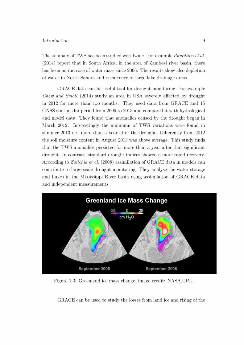
sea level. Figure 1.3 illustrates the changes in Greenland’s ice mass as measuredby GRACE and analysed by international researchers for the period betweenSeptember 2005 (left) and September 2008 (right). The study is led by theDenmark National Space Institute in Copenhagen. The research indicates thatthe ice-loss acceleration began moving up the northwest coast of Greenland inlate 2005. The team drew their conclusions by comparing data from GRACEwith continuous GPS measurements made from long-term sites on bedrock onthe edges of the ice sheet. Obviously apart of the losses there is increasing ofthe ice mass in the central area of Greenland. Figure 1.4 shows the amount oftotal mass change processed by Princeton researchers. The plot is extractedfrom Harig and Simons (2012) and shows that Greenland experienced a steadyice loss of 200 Gt annuallyGardner et al. (2013) show that in many regions,local measurements give larger ice mass losses than satellite-based estimates.The largest mass losses for the 2003-2009 period form GRACE are in ArcticCanada, Alaska, coastal Greenland, the southern Andes, and high-mountainAsia, but there was little loss from glaciers in Antarctica. Over the research
Introduction 11
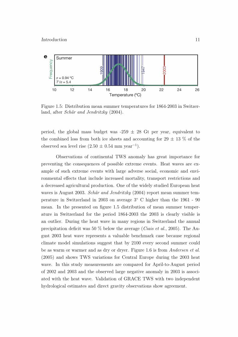
Figure 1.5: Distribution mean summer temperatures for 1864-2003 in Switzer-land, after Schär and Jendritzky (2004).
period, the global mass budget was -259 ± 28 Gt per year, equivalent tothe combined loss from both ice sheets and accounting for 29 ± 13 % of theobserved sea level rise (2.50 ± 0.54 mm year−1).
Observations of continental TWS anomaly has great importance forpreventing the consequences of possible extreme events. Heat waves are ex-ample of such extreme events with large adverse social, economic and envi-ronmental effects that include increased mortality, transport restrictions anda decreased agricultural production. One of the widely studied European heatwaves is August 2003. Schär and Jendritzky (2004) report mean summer tem-perature in Switzerland in 2003 on average 3◦ C higher than the 1961 - 90mean. In the presented on figure 1.5 distribution of mean summer temper-ature in Switzerland for the period 1864-2003 the 2003 is clearly visible isan outlier. During the heat wave in many regions in Switzerland the annualprecipitation deficit was 50 % below the average (Ciais et al., 2005). The Au-gust 2003 heat wave represents a valuable benchmark case because regionalclimate model simulations suggest that by 2100 every second summer couldbe as warm or warmer and as dry or dryer. Figure 1.6 is from Andersen et al.(2005) and shows TWS variations for Central Europe during the 2003 heatwave. In this study measurements are compared for April-to-August periodof 2002 and 2003 and the observed large negative anomaly in 2003 is associ-ated with the heat wave. Validation of GRACE TWS with two independenthydrological estimates and direct gravity observations show agreement.
Introduction 12
Figure 1.6: 2003 TWS anomaly for Central Europe, after Andersen et al.(2005).
Monitoring of water vapour and TWS is of interest in South-east Eu-rope, since the heat waves are a common summer feature in the region. Forexample, the heat wave in July 2007 had large geographical extension reach-ing Bulgaria. The heat wave continued six days from 19 to 25 July. Theatmospheric circulation leading to the heat wave is characterized by northerlydisplacement of the subtropical jet stream allowing the subtropical African airto reach the Balkan Peninsula as far as 50◦ N. On figure 1.7 is shown the airtongue spreading over the Mediterranean sea and Balkan Peninsula at 00 UTCon 23 July 2007.
The aim of this thesis is to investigate the anomalies of observed andmodelled temperature, precipitation, IWV and TWS during the 2007 heatwave inSouth-east Europe. In chapter 2 are presented the data and the methodused. Chapter 3 and 4 presents the 2007 anomalies of temperature, precipita-tion, IWV and TWS in observations and model, respectively. The conclusion
Introduction 13
Figure 1.7: Temperature at 850 hPa (1.5 km msl.) on 23 July 2007 00 UTC.,after Simeonov et al. (2013).
are given in Chapter 5.
Chapter 2
Data and methods
In this work are used surface and satellite observations in combination withsimulations with a regional climate model ALADIN-Climate. The observationand simulations are archived in the Sofia University Atmospheric Data Archive(Guerova et al., 2014). On figure 2.1 is shown the scheme of the data used inthis work. The first column is for the ALADIN-Climate simulations describedin section 2.4, the second is for the data flow of GNSS derived IWV (see section2.3). It is to be noted that SYNOP observations (see the arrow in figure 2.1)are used to obtain GNSS IWV. The surface observations from synoptic station(SYNOP) are in column three (see section 2.2) and the GRACE data set is incolumn four (see section 2.1).
ALADIN − Climate
extract
��
IGS
extract
��
Ogimet
extract
��
GRACE
extract
��1D parameter
T [C],IWV [mm],pp[mm],TWS[kg/m2]
��
GNSS
ZTD[mm]
SY NOP
T [K],p[hPa],r[mm/12h]
��
1D parameter
TWS[m]
��GCM
��
GNSS_OUT
��
SY NOP
ww ��
GRACE
��Tm PPm IWVm TWSm GNSS IWV T PP TWS
Figure 2.1: SUADA table names and data flow used in this thesis.
14
Data and methods 15
2.1 GRACE data
GRACE satellite mission is a cooperation between the National Aeronauticsand Space Administration (NASA) and the German Research Centre for Geo-sciences (GFZ). GRACE mission is of two identical satellites that fly 220 kmapart on a polar orbit at 500 km above surface. Figure 2.2 illustrates theGRACE twin satellite connected with highly precise K-band microwave sys-tem which measures the gravity anomaly as a change in the distance betweenthe satellites. Such variations in the distance between the satellites are pos-sible when the lead spacecraft passes above large concentration of mass i.e.a stronger gravity pulls it away from the second GRACE satellite behind inthe same orbital plane. These measurements, along with GNSS based locationinformation are used to compute monthly gravity field solutions (web, d).
Figure 2.2: GRACE mission - twin satellites on polar orbit (500 km) connectedwith laser link, image credit: web (a).
In figure 2.3 is presented the GRACE processing scheme. The satellite
Data and methods 16
orbits are processed in daily arcs. For each arc initial conditions, stochas-tic accelerations and accelerometer scale factors are estimated (Level 1 data).The spherical harmonic coefficients of the gravity field are set up togetherwith the arc-specific parameters. The daily Normal EQuations (NEQs) withrespect to the kinematic orbits of GRACE satellites and with respect to theK-Band range-rate observations are combined and the arc-specific parametersare pre-eliminated from the combined NEQs. Finally the reduced NEQs areaccumulated to monthly batches to solve for the gravity model parameters.The result are mathematical functions defined on surface of a sphere - spher-ical harmonics, which solutions are spherical harmonic coefficients. GRACEcoefficients are objective mainly for continental water storage (Level 2 data),but also include errors from the correction models and noise (Swenson andWahr , 2006).
The temporal variations of the gravity filed over the continents are at-tributed to: 1) the hydrological cycle, 2) ice mass changes in the polar, subpolarregions and large glaciers, and 3) post glacial rebound. Using a priori modelsof known gravitational accelerations the static gravity field of the Earth, whichrepresents 99 % of the observed signal, its time variations are removed. Polarmovements, atmosphere and ocean mass changes also are removed in order toanalyse the continental hydrology component of water storage. For this pur-pose are used global ocean circulation models and reanalysis from EuropeanCentre for Medium-Range Weather Forecasts (ECMWF) and National Centresfor Environmental Prediction (NCEP).
In this study is used GRACE Level 2 monthly gravity variations, repre-sented in equivalent water height. The variations were computed from GRACEsatellite observations and derived from Astronomical Institute at University ofBern (AIUB-RL02) series of monthly gravity fields (Meyer et al., 2016). Valuesare calculated within a radius of 300, 500 and 700 km around Sofia. A Gaus-sian bell curve was applied for weighting. The radius given is the half widthradius of the Gaussian bell curve, which is a common procedure for smoothingof GRACE derived gravity models.
Data and methods 17
Level 1GRACE observation
velocities and position (GPS)accelerometer data
inter-satellite K-Band range
��Residuals of observationfor continental hydrology
��Partial derivatives
of observations versusspherical harmonics
��Normal equations
(First order)
��Stokes Coefficients
��Level 2
Terrestrial water storage anomaly(TWS anomaly)
Figure 2.3: GRACE processing scheme for TWS derivation.
2.2 Surface synoptic data
In this thesis are used surface synoptic observations (SYNOP) of temperatureand precipitation from Sofia station of the National Institute of Meteorologyand Hydrology (NIMH). The data is acquired from OGIMET, which is an on-line weather information server, and is uploaded in SUADA. Data is placedat SYNOP table of the database. The SYNOP table contains unprocessedmeteorological data. The surface temperature (T) and precipitation (PP) areextracted from SUADA and monthly mean time series and anomalies are com-puted using MATLAB and R programs. Errors of the observation are ± 0.1◦
C for temperature and ± 0.5 mm for precipitation.
Data and methods 18
2.3 GNSS tropospheric products
The GNSS tropospheric products are from the first processing campaign ofthe International GNSS Service (IGS) (Byun and Bar-Sever , 2009; Rebischunget al., 2012). IGS is a scientific consortium from over 200 worldwide nationalagencies, universities and research institutions from more than 80 countries. Itcomputes and maintains a global network of over 350 permanent, continuouslyoperated GNSS sites. IGS provides data for total tropospheric delay in zenithdirection (ZTD). The GNSS station in Sofia (SOFI) is processed since 1997.The SUADA contains continuous GNSS data for SOFI from 1997 to 2015. Toderive IWV from the ZTD the 2 meter surface pressure (ps) and temperature(ts) from SYNOP are used as bellow:
ZWD = ZTD − 2.2768ps
1− 0.00266cos(2θ)− 0.00028h(2.1)
IWV =106
(k3/Tm + k2)Rv
ZWD, (2.2)
where k2, k3 and Rv are constant, Tm is the weighted mean atmospheric tem-perature, h is the height and θ is the latitude variation of the gravitationalacceleration.
After computing the IWV values they are stored in GNSS_OUT tableof SUADA. Errors of the GNSS IWV are less than 1 mm.
2.4 Regional climate model ALADIN-Climate
ALADIN-Climate is a Regional Climate Model (RCM) developed in an inter-national cooperation at Mètèo France. It was created merging the dynamicsof the numerical weather prediction model ALADIN and the parameteriza-tion schemes from ARPEGE-Climate global climate model. The currentlyused version of ALADIN-Climate is described in Csima and Horányi (2008).ALADIN-Climate parameterization schemes include: 1) Fouquart and Mor-crette radiation scheme (Morcrette, 1989), 2) ISBA land scheme (Noilhan and
Data and methods 19
Planton, 1989) of four layers of soil temperature without a deep relaxation,two soil moisture layers (with parameterization of soil freezing) and a singlelayer snow model (with variable albedo and density), based on Douville et al.(1995), 3) deep convection scheme designed according to Bougeault (1985),4) cloud scheme by Ricard and Royer (1993), and 5) large-scale precipitationscheme following Smith (1990). Lateral boundary conditions for ALADIN-Climate simulation are from ERA-Interim reanalysis developed at ECMWFand described in (Dee et al., 2011). The RCM is integrated over the EURO-CORDEX domain presented in figure 2.4 for the hindcast period of 1989-2008.ALADIN-Climate spatial resolution is 50 km (0.44◦) with 31 vertical levels.
Figure 2.4: ALADIN-Climate RCM domain.
In this work ALADIN-Climate data are used for the period 2003-2008since it is the only common set with the observations. Data is achieved in
Data and methods 20
SUADA database in table GCM. Extracted is one model grid point with lati-tude 42◦ 25’ N, longitude 23◦ 25’ E and altitude 1130 m asl. In table 2.1 areshown ALADIN-Climate model coordinates and those of SYNOP station Sofiaand GNSS station SOFI.
Station name longitude (East) latitude (North) altitude (m asl)SYNOP-Sofia 23◦ 35’ 42◦ 41’ 590GNSS-SOFI 23◦ 25’ 42◦ 29’ 1120ALADIN-Cl. 23◦ 25’ 42◦ 25’ 1130
Table 2.1: Coordinates of observation and model grid point.
Chapter 3
Observation anomalies: 2007 vs2003-2013
In this section observations from SYNOP, GNSS and GRACE are presentedfor period 2003-2013.
3.1 Temperature and precipitation anomaly from
observations
On figure 3.1 a, b, c, d are shown: 1) monthly mean temperatures time series, 2)moving average of length 6, 3) monthly mean temperatures for 2007 comparedwith period 2003-2013, and 4) monthly anomalies for 2007. As can be seenfrom figure 3.1a the temperature has an annual cycle. The peak is in summermonths - June, July and August and minimum is in winter time - Decemberand January. On figure 3.1b is filtered data by moving average of length 6.By this filter are smoothed high frequency variations and is reduced the effectof all cycles with periods smaller or equal to six months. Clearly seen is thesteady increase of temperature trend in the summer of 2007. When comparedto 2003-2013 mean (3.1c, dashed line), it is obvious that temperature in first8 months of 2007 are higher. Next months to the end of 2007 the temperature
21
Results 22
is lower than the 2003-2013 monthly means. From figure 3.1d is seen that thetemperature anomaly in July 2007 is positive - 2.3◦ C above 2003-2013 mean.Interestingly the largest positive anomaly is in January - almost 5.4◦ C abovethe 2003-2013 mean.
Figure 3.2 presents: 1) precipitation time series, 2) moving averageof length 6, 3) monthly mean precipitation for 2007 compared with period2003-2013, and 4) precipitation anomaly for 2007. According to figure 3.2aprecipitation time series do not show annual cycle. There are more than onepeak per year. Maximums of precipitation appear in the end of spring (May,early summer June) and autumn (September and October), although thereare some exceptions. In 2005 the peaks are in winter (December) and summer(August). In 2009 again precipitation maximums appears in winter (January)and summer time (August). Winter maximum can be seen again in December2010, January 2012 and February 2013. Most of the minimums can be noticedin spring (Mart and April) and in the end of autumn (November). Significantminimums in the end of winter and early spring are obtained in February 2008and 2009 and in March 2003 and 2012. Large summer minimums are seenonly in August 2003, July 2007 and August 2008. In summary this figureshows the irregular behaviour of precipitation, but it can be said that thelarge peaks are slowly moved from early spring and autumn to winter andsummer, respectively. In addition it can be seen that the amplitude of peaksbecomes smaller over time. This is confirmed in figure 3.2b. The filtered data ofprecipitation show decrease after 2006. At figure 3.2c is shown monthly meanprecipitation for 2007 (white bars) and 2003-2013 (green bars). Maximum for2003-2013 monthly mean precipitation is 85 mm in June with a minimum of30 mm in November. In 2007 the monthly mean precipitation reaches 175 mmin May and 5 mm in July. The anomalies are plotted in figure 3.2d. In July2007 precipitation anomaly reached -60 mm - the absolute minimum for thisyear. In January 2007 the precipitation is in the norm.
Results 23
3.2 IWV anomaly from observations
On figure 3.3a, b, c, d are shown: 1) monthly mean IWV time series, 2) mov-ing average of length 6, 3) monthly mean IWV for 2007 and 2003-2013 and 4)monthly anomalies for 2007, respectively. From 3.3a is seen that, similar tothe temperature, monthly mean IWV has annual cycle. Each year starts withupward trend and peaks in summer (June, July or August) followed by down-ward trend and minimum in winter season (December, January or February).Also according to 3.3a the minimums as well as the maximums of IWV in-crease their amplitude almost each following year. On figure 3.3b is shown theIWV moving average with length 6. As it can be seen the lowest IWV valuesare in the end of 2006 and the beginning of 2007. Large maximum is recordedin summer 2009. On figure 3.3c is shown the monthly mean IWV values for2007 (thick line) versus 2003-2013 (dashed line). In first four months of 2007IWV is constant then increases in May. Clearly IWV in July 2007 is smallerthan 2003-2013. Until the end of 2007 IWV is below or close to the norm. Onfigure 3.3d is plotted the IWV anomaly and the first negative anomaly is inApril followed by July, September and December. Positive anomaly in May is2 mm above the mean for 2003-2013 period. The largest negative anomaly isin July and is 3.5 mm under the norm.
3.3 TWS anomaly from observations
Figure 3.4 a, b, c, d shows: 1) TWS anomaly time series, 2) moving averageby length 6, 3) monthly mean TWS anomalies and, and 4) 2007 anomaly. Onfigure 3.4a is shown TWS variations in centimetres for ten year period from2003 to 2013 for 3 smoothing radii - 300 km (R1 - black line), 500 km (R2 -red line), and 700 km (R3 - blue line). As can be seen the TWS variationshave annual cycle. Each year starts with upward trend of TWS anomaly andafter passing its peak in February, March or April a downward trend leads tothe minimum in August, September or October. Then in next months TWSstarts to increase again. What differs every year is the amplitude of TWSanomaly. Also the maximums and minimums are indicative for significant
Results 24
changes in some of the water cycle components. For example the minimum ofmore than -15 cm (for R1) in the TWS anomaly trend that appears in 2003 islikely linked to the heat wave occurred in Europe. Second lowest magnitudeof TWS variations is noticed in summer of 2007. In August, a month afterappearance of Balkan heat wave TWS value reached -10 cm. On figure 3.4bis seen moving average of length 6 for GRACE data using only the radius of300 km. Clearly seen is the negative TWS trend in summer months of 2007.The largest negative TWS anomaly is also in summer 2007 (figure 3.4c). InAugust 2007 TWS anomaly has a minimum of -10 cm. All months in 2007,with exception of November and December, have negative TWS anomaly orare close to the mean.
Results 25
Figure 3.1: (a) Temperature time series for period 2003-2013; (b) movingaverage of length 6; (c) monthly mean temperatures for 2003-2013 (dashedline) and for 2007 (thick line); (d) anomalies for 2007 versus 2003-2013.
Results 26
Figure 3.2: (a) Precipitation time series for period 2003-2013; (b) movingaverage of length 6; (c) monthly mean precipitation for 2003-2013 (dashedline) and for 2007 (thick line); (d) precipitation anomalies for 2007 versus2003-2013.
Results 27
Figure 3.3: (a) IWV time series for period 2003-2013; (b) moving average oflength 6; (c) monthly mean IWV for 2003-2013 (dashed line) and for 2007(thick line); (d) IWV anomalies for 2007 versus 2003-2013.
Results 28
Figure 3.4: (a) TWS variations time series for period 2003-2013 with smoothingradii of 300 km (R1 - black line), 500 km (R2 - red line) and 700 km (R3 -blue line); (b) moving average of length 6; (c) monthly mean TWS changesfor 2003-2013 (dashed line) and for 2007 (thick line); (d) TWS anomalies for2007 versus 2003-2013.
Chapter 4
RCM anomalies: 2007 vs2003-2008
In this section observations from SYNOP, GNSS and GRACE are comparedwith ALADIN-Climate model simulations. All data is processed for period2003-2008. On plots are presented monthly anomalies in 2007 when comparedto 2003-2008, for both observation and model. Correlation coefficient of tem-perature, precipitation, IWV and TWS pairs is given in table 3.2.
4.1 Temperature and precipitation anomaly RCM
At figure 4.1a are shown monthly temperature anomalies for 2007 from SYNOPobservation (black circles) and ALADIN-Climate model (red circles). In theSYNOP data first eight months of 2007 are with positive temperature anomalyand the remaining four are with negative. Large positive anomaly occurs inJanuary - above 5◦ C. In July the anomaly reaches up to 3◦ C. Only onedifference in ALADIN-Climate model is seen with a negative anomaly in April.The month with highest temperature anomaly (5◦ C) in ALADIN-Climate isin June. When compared the result the following features stand out: 1) largepositive temperature anomaly in January, 2) positive anomaly in July, and3) large negative anomaly in November. The model data results are in good
29
Results 30
agreement with SYNOP observations and correlation is 0.70.
On figure 4.1b are shown monthly precipitation anomalies for 2007.When compared the following features stand out: 1) in first quarter (January-March) precipitation anomalies are in good agreement and the amplitude dif-ferences are in the range of 10 mm, 2) in the next quarter the precipitationanomalies have big discrepancy, 3) both data sets have negative anomaly inJuly, and 4) precipitation anomalies are in agreement for the next months withexception of September. Here the mismatches are more than the coincidences,although in July precipitation anomaly is negative and then is positive in Au-gust in both observation and RCM. Correlation coefficient for precipitationanomaly data pair is 0.32, which indicates poor agreement.
4.2 IWV anomaly RCM
Monthly IWV anomalies are shown on figure 4.2 Again two methods are com-pared - GNSS data from station SOFI (black circles) and ALADIN-Climatemodel (red circles). When compared results the following features stand outfor 2007: 1) positive IWV anomaly in February, 2) negative IWV anomaly inApril, and 3) negative IWV anomaly in July. According to GNSS data theminimum value of IWV anomaly is in July(- 3 mm), while for the model min-imum is in September (-2 mm). The correlation coefficient of 0.73 suggestsstrong relation between GNSS and RCM.
4.3 TWS anomaly RCM
Monthly TWS anomalies from GRACE (black circles) and ALADIN-Climatemodel (red circles) are shown on figure 4.3 When compared the following fea-tures stand out for 2007: 1) downward trend of TWS anomaly from Februaryto May, 2) TWS is in range of 1 cm in June, and 3) large differences in thesecond half of the year after June. There is not a good agreement between thedata. That is confirm from the correlation coefficient of -0.68. Although the
Results 31
year/corr T P IWV TWS2007 0.70 0.32 0.73 -0.68
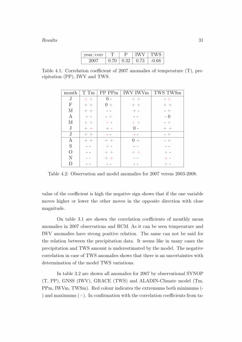
Table 4.1: Correlation coefficient of 2007 anomalies of temperature (T), pre-cipitation (PP), IWV and TWS.
Table 4.2: Observation and model anomalies for 2007 versus 2003-2008.
value of the coefficient is high the negative sign shows that if the one variablemoves higher or lower the other moves in the opposite direction with closemagnitude.
On table 3.1 are shown the correlation coefficients of monthly meananomalies in 2007 observations and RCM. As it can be seen temperature andIWV anomalies have strong positive relation. The same can not be said forthe relation between the precipitation data. It seems like in many cases theprecipitation and TWS amount is underestimated by the model. The negativecorrelation in case of TWS anomalies shows that there is an uncertainties withdetermination of the model TWS variations.
In table 3.2 are shown all anomalies for 2007 by observational SYNOP(T, PP), GNSS (IWV), GRACE (TWS) and ALADIN-Climate model (Tm,PPm, IWVm, TWSm). Red colour indicates the extremums both minimums (-) and maximums (+). In confirmation with the correlation coefficients from ta-
Results 32
ble 3.1, there is a good agreement between the SYNOP and ALADIN-Climatemodel as well as between the GNSS and RCM. The negative correlation be-tween GRACE and ALADIN-Climate is also confirmed by this table. Obvi-ously in almost each month the direction of GRACE TWS anomaly is oppositefrom the model results.
Results 33
Figure 4.1: Temperature (top) and precipitation anomalies (bottom) for 2007from SYNOP observations (black circles) and ALADIN-Climate model (redcircles).
Results 34
Figure 4.2: IWV anomaly for 2007 from observations (black circles) andALADIN-Climate model (red circles).
Figure 4.3: TWS anomaly for 2007 from observations (black circles) andALADIN-Climate model (red circles).
Chapter 5
Conclusions
In this thesis the synergy between surface and satellite observations is usedto study the behaviour of three components of the hydrology cycle namely,precipitation, water vapour and terrestrial water storage during the July 2007heat wave in South-east Europe. The e anomalies of temperature, precipi-tation, IWV and TWS in 2007 as compared to 2003-2013 indicate relationbetween them and the occurrence of the heat wave in July. Surface obser-vations show positive temperature anomalies for first eight months of 2007.The heat wave month (July 2007) was 2◦ C hotter than the 2003-2013 meanin Sofia, Bulgaria. There are significant negative precipitation anomalies inMarch, April and July 2007. According to GNSS data the minimum of IWV isin July 2007. GRACE data is in good agreement with the surface and GNSSresults and show minimums in spring and summer. The absolute minimum ofTWS anomaly is in August i.e. a month after the occurrence of the heat wave,possibly due to the slower response of the soil to the heating.
In addition the observed anomalies in 2007 are compared to simulationswith the regional climate model ALADIN-Climate. The comparison betweenanomalies from observations and ALADIN-Climate model gives: 1) strongcorrelation for temperature and IWV between the two data sets, and 2) weakrelation between the precipitation and TWS anomalies data set. The compar-ison shows that the precipitation and TWS amount tend to be underestimatedin the model. Precipitation and terrestrial water storage are very difficult to
35
Conclusions 36
simulate thus assimilation of GRACE observations in the climate model canbe a possible way to correct this deficiency.
The result of using GRACE data shows that there is strong capaci-ties of multi-satellite observations to monitor quantitatively the changes in thestorage of surface and sub-surface reservoirs associated with climate variabil-ity and human activities at a regional scale. In the near future the remotelysensed data sets like GRACE are likely to have large impact in regions likeBulgaria where in situ data are sparse. University of Bern is currently coordi-nating a project aiming to set European Gravity Service for Improved Emer-gency Management (EGSIEM, Jaeggi (2015)). EGSIEM objectives are: 1) todeliver the best time-variable gravity products for applications in Earth andenvironmental science research, 2) to reduce the latency and to increase thetemporal resolution of the gravity and related mass redistribution products,and 3) to develop gravity-based indicators for extreme hydrological events anddemonstrate their value for flood and drought forecasting and monitoring ser-vices. Primary input to EGSIEM is the GRACE and GRACE-FO (Follow-on,NASA-GFZ, due for launch in 2017) satellite mission data.
Acknowledgement 37
Acknowledgement
I would like to thank to:
• Assoc. prof. Guergana Guerova for being my thesis supervisor andhelping me during my study.
• Tzvetan Simeonov for his help with operating SUADA and GNSSprocessing.
• Dr. Ulrich Meyer, from the University of Bern for providing GRACEdata.
• Peter Szabo from the Hungarian Meteorological Service for providingALADIN-Climate data.
Bibliography
University of Texas at Austin center for space research, http://csr.utexas.edu/grace/publications/brochure/page11.html, a.
Global terrestrial observation system, http://www.fao.org/gtos/
gt-nethyd.html, b.
Global TWS anomaly, http://www.globalwaterforum.org/wp-content/
uploads/2013/08/Figure-3.png, c.
Gravity Recovery And Experiment, http://nasa.gov/Grace, d.
GRACE Follow-On, http://gracefo.jpl.nasa.gov, e.
Andersen, O. B., S. I. Seneviratne, J. Hinderer, and P. Viterb, GRACE-derived terrestrial water storage depletion associated with the 2003European heat wave, Geophysical research letters, 32, L18,405,doi:10.1029/2005GL023574, 2005.
Bougeault, P., A simple parameterization of the large-scale effects of cumulusconvection, Monthly Weather Review, 113 (12), 2108–2121, 1985.
Byun, S. H., and Y. E. Bar-Sever, A new type of troposphere zenith path delayproduct of the international GNSS service, Journal of Geodesy, 83 (3-4),1–7, 2009.
Chew, C. C., and E. E. Small, Terrestrial water storage response to the 2012drought estimated from GPS vertical position anomalies, 2014.
Ciais, P., et al., Europe-wide reduction in primary productivity caused by theheat and drought in 2003, Nature, 437 (7058), 529–533, 2005.
38
bibliography 39
Csima, G., and A. Horányi, Validation of the ALADIN-Climate regional cli-mate model at the Hungarian meteorological service, Időjárás, 112 (3-4),155–177, 2008.
Dai, A., Recent climatology, variability, and trends in global surface humidity,Journal of Climate, 19 (15), 3589–3606, 2006.
Dee, D., et al., The ERA-Interim reanalysis: Configuration and performanceof the data assimilation system, Quarterly Journal of the Royal Meteoro-logical Society, 137 (656), 553–597, 2011.
Douville, H., J.-F. Royer, and J.-F. Mahfouf, A new snow parameterization forthe Meteo-France climate model, Climate Dynamics, 12 (1), 21–35, 1995.
Gardner, A. S., G. Moholdt, J. G. Cogley, B. Wouters, and F. Paul, A rec-onciled estimate of glacier contributions to sea level rise: 2003 to 2009,Science, 304, 852–857, 2013.
Guerova, G., T. Simeonov, and N. Yordanova, The sofia university atmosphericdata archive (suada), Atmospheric Measurement Techniques, 7 (8), 2683–2694, 2014.
Harig, C., and F. J. Simons, Mapping Greenland’s mass loss in space and time,Proceedings of the National Academy of Sciences, 109 (49), 19,934–19,937,2012.
Jaeggi, A., European gravity service for improved emergency management-project overview and first results, in 2015 AGU Fall Meeting, Agu, 2015.
Matzarakis, A., C. De Freitas, and D. Scott, Developments in tourism climatol-ogy, in 3rd International Workshop on Climate, Tourism and Recreation,Freiburg, Citeseer, 2007.
Meyer, U., A. Jäggi, Y. Jean, and G. Beutler, AIUB-RL02: an improved timeseries of monthly gravity fields from GRACE data, Geophysical JournalInternational, p. ggw081, 2016.
Morcrette, J.-J., Description of the radiation scheme in the ECMWF model,European Centre for Medium-Range Weather Forecasts, 1989.
bibliography 40
Noilhan, J., and S. Planton, A simple parameterization of land surface pro-cesses for meteorological models, Monthly Weather Review, 117 (3), 536–549, 1989.
Ramillien, G., F. Frappart, and L. Seoane, Application of the regional watermass variations from GRACE satellite gravimetry to large-scale watermanagement in Africa, Remote sensing, 6, 2014.
Rebischung, P., J. Griffiths, J. Ray, R. Schmid, X. Collilieux, and B. Garayt,IGS08: the IGS realization of ITRF2008, GPS solutions, 16 (4), 483–494,2012.
Ricard, J., and J. Royer, A statistical cloud scheme for use in an AGCM, inAnnales Geophysicae, vol. 11, pp. 1095–1115, 1993.
Schär, C., and G. Jendritzky, Climate change: hot news from summer 2003,Nature, 432 (7017), 559–560, 2004.
Simeonov, T., K. Vassileva, and G. Guerova, Application of ground-basedGNSS meteorology in Bulgaria/Southeast Europe: case study 2007 heatwave, Annual of University of Sofia, 106, 88–100, 2013.
Smith, R., A scheme for predicting layer clouds and their water content in ageneral circulation model, Quarterly Journal of the Royal MeteorologicalSociety, 116 (492), 435–460, 1990.
Stocker, et al., IPCC, 2013: Climate Change 2013: The Physical ScienceBasis. Contribution of Working Group I to the Fifth Assessment Reportof the Intergovernmental Panel on Climate Change, Cambridge UniversityPress, Cambridge, United Kingdom and New York, NY, USA, 2013.
Swenson, S., and J. Wahr, Post-processing removal of correlated errors inGRACE data, Geophys. Research Lett., 33, 2006.
Trenberth, K. E., L. Smith, T.Qian, and J. Fasullo, Estimates of the globalwater budget and its annual cycle using observational and model data, 8,2006.
bibliography 41
Zaitchik, B. F., M. Rodell, and R. H. Reichle, Assimilation of GRACE ter-restrial water storage data into a land surface model: Results for theMississippi river basin, Journal of Hydrometeorology, 9, 535–548, 2008.