tesi.cab.unipd.ittesi.cab.unipd.it/43646/1/Tesi_Magistrale_Janjic.pdf · La sequenza di onde...

Design of an In-Vitro Set-up for Sonothrombolysis of human blood clots using

microbubbles

J O V A N A J A N J I C

Supervisor at UNIPD: Alfredo Ruggeri Supervisors at KTH: Anna Bjällmark, Malin Larsson

Università degli studi di Padova UNIPD

http://www.unipd.it

Royal Institute of Technology KTH STH

SE-141 86 Flemingsberg, Sweden http://www.kth.se/sth

Acknowledgments

I would like to start by thanking my supervisors Anna Bjällmark and Malin Larsson, for the help,guidance and constructive comments in all the stages of the thesis work.

Special thanks also to all my friends that have shared with me the invaluable experience of Erasmus,supporting me in all the di�cult moments.

Last but not the least, I wish to express my love and gratitude to my family and to my boyfriendEnrico for their understanding and endless love through the duration of my studies.

i

ii

Abstract

Several studies suggest that the use of ultrasound in conjunction with microbubbles (MBs) caninduce the lysis of the blood clots through acoustic cavitation and through the production ofmicrojets and microstreaming. However, there is no accordance about the optimal ultrasoundparameters that have to be considered in order to achieve the maximum thrombolytic e�ect, neithera clear agreement about the type of MBs that have to be used.

This project had two main goals: the design and optimization of an in-vitro set-up for thestudy of clot lysis within coronary arteries and its testing with ultrasound in conjunction with twodi�erent types of MBs. The MBs considered were the 3MiCRON MBs and the SonoVue MBs.

The ultrasound sequence was developed using a programmable ultrasound architecture (Vera-sonics, Inc) and was tested using commercially available clinical transducers.

Using the designed set-up and varying the ultrasound parameters (frequency, pulse length andpulse amplitude) it was possible to study the clot lysis e�ciency in conjunction with the two types ofMBs. For the 3MiCRON MBs no increase in clot lysis was found with the implemented ultrasoundparameters, while considering the SonoVue MBs, a 10% increase in clot lysis was found with 10mslong pulse delivered at 50V (peak-to peak value).

The obtained set-up had several aspects in common with the real situation of occluded coronaryarteries, although some limitations were present and further optimizations are required.

Further work is required in order to assess if di�erent combination of ultrasound parameters areable to lead to an increase in clot lysis when delivered with 3MiCRON or SonoVue MBs.

iii

iv

Sommario

Diversi studi suggeriscono che l'utilizzo di ultrasuoni e di microbolle (agenti di contrasto) puòindurre la lisi di trombi sanguigni attraverso il fenomeno della cavitazione acustica e tramite laproduzione di microgetti e microvortici. Tuttavia, non vi è un comune accordo su quali siano iparametri ultrasonori ottimali nè le microbolle da utilizzare al �ne di ottenere il massimo e�ettotrombolitico.

Questo lavoro di tesi presenta due obiettivi fondamentali: la progettazione ed ottimizzazione diun sistema in-vitro per lo studio della lisi dei trombi all'interno delle arterie coronarie e l'utilizzo ditale sistema in concomitanza con l'applicazione di ultrasuoni e di microbolle. Due tipi di microbollesono state prese in esame: 3MiCRON e SonoVue.

La sequenza di onde ultrasonore è stata sviluppata tramite un'architettura programmabile (Ve-rasonics, Inc) ed è stata trasmessa usando trasduttori clinici presenti in commercio .

Utilizzando il sistema sviluppato e variando i parametri ultrasonori (frequenza, lunghezza eampiezza dell'impulso) è stato possibile studiare l'e�cienza trombolitica degli ultrasuoni con i duetipi di microbolle. Applicando le microbolle 3MiCRON non è stato riscontrato alcun miglioramentonella lisi dei trombi, mentre considerando le microbolle SonoVue è stato notato un aumento dellatrombolisi del 10%, trasmettendo impulsi ultrasonori della durata di 10ms a 50V (valore picco-picco).

Il sistema progettato ha diversi aspetti in comune con la situazione reale di occlusione dellearterie coronarie, sebbene siano presenti alcune limitazioni e ulteriori studi di ottimizzazione sianonecessari.

Studi aggiuntivi sono inoltre necessari al �ne di chiarire se diverse combinazioni di parametriultrasonori siano capaci di condurre ad un aumento della trombolisi in combinazione con i due tipidi microbolle considerati.

v

vi

Contents

Introduction x

1 Background 11.1 Thrombosis . . . . . . . . . . . . . . . . . . . . . . . . . . . . . . . . . . . . . . . . . 1

1.1.1 Arterial Thrombosis . . . . . . . . . . . . . . . . . . . . . . . . . . . . . . . . 21.1.1.1 Coronary circulation and myocardial infarction . . . . . . . . . . . . 21.1.1.2 Ischemic Stroke . . . . . . . . . . . . . . . . . . . . . . . . . . . . . 31.1.1.3 Systemic embolism . . . . . . . . . . . . . . . . . . . . . . . . . . . . 4

1.1.2 Venous thrombosis . . . . . . . . . . . . . . . . . . . . . . . . . . . . . . . . . 41.1.2.1 Deep Venous thrombosis . . . . . . . . . . . . . . . . . . . . . . . . 5

1.2 Ultrasound principles . . . . . . . . . . . . . . . . . . . . . . . . . . . . . . . . . . . . 61.2.1 Ultrasound Physiscs . . . . . . . . . . . . . . . . . . . . . . . . . . . . . . . . 61.2.2 Ultrasound interaction with tissue . . . . . . . . . . . . . . . . . . . . . . . . 7

1.2.2.1 Re�ection . . . . . . . . . . . . . . . . . . . . . . . . . . . . . . . . . 71.2.2.2 Refraction . . . . . . . . . . . . . . . . . . . . . . . . . . . . . . . . 71.2.2.3 Attenuation . . . . . . . . . . . . . . . . . . . . . . . . . . . . . . . 8

1.2.3 Non linear propagation . . . . . . . . . . . . . . . . . . . . . . . . . . . . . . 81.2.4 Contrast agents . . . . . . . . . . . . . . . . . . . . . . . . . . . . . . . . . . . 10

1.3 Sonothrombolysis . . . . . . . . . . . . . . . . . . . . . . . . . . . . . . . . . . . . . . 121.3.1 Mechanisms of action and MBs in�uence . . . . . . . . . . . . . . . . . . . . . 121.3.2 Ultrasound thrombolysis techniques . . . . . . . . . . . . . . . . . . . . . . . 13

1.3.2.1 Catheter-delivered ultrasound thrombolysis . . . . . . . . . . . . . . 141.3.2.2 Transcutaneous-delivered HIFU external ultrasound . . . . . . . . . 141.3.2.3 Surface ultrasound delivery . . . . . . . . . . . . . . . . . . . . . . . 15

1.3.3 Safety and e�ciency aspects of Sonothrombolysis . . . . . . . . . . . . . . . . 15

2 Design, validation and optimization of the in-vitro set-up 172.1 Methods . . . . . . . . . . . . . . . . . . . . . . . . . . . . . . . . . . . . . . . . . . . 172.2 Results . . . . . . . . . . . . . . . . . . . . . . . . . . . . . . . . . . . . . . . . . . . . 232.3 The �nal in-vitro set-up . . . . . . . . . . . . . . . . . . . . . . . . . . . . . . . . . . 25

3 Clot lysis tests with ultrasound and MBs 273.1 Methods . . . . . . . . . . . . . . . . . . . . . . . . . . . . . . . . . . . . . . . . . . . 27

3.1.1 Production of 3MiCRON MBs . . . . . . . . . . . . . . . . . . . . . . . . . . 283.1.2 Production of SonoVue MBs . . . . . . . . . . . . . . . . . . . . . . . . . . . 28

vii

viii CONTENTS

3.1.3 Implemented protocols for ultrasound transmission . . . . . . . . . . . . . . . 293.1.3.1 Control tests: no MBs and no ultrasound application . . . . . . . . 303.1.3.2 3MiCRON and high frequency exposure . . . . . . . . . . . . . . . . 303.1.3.3 3MiCRON/SonoVue and low frequency exposure . . . . . . . . . . 313.1.3.4 SonoVue with longer pulse and lower voltage exposure . . . . . . . . 33

3.1.4 The Verasonics system . . . . . . . . . . . . . . . . . . . . . . . . . . . . . . . 343.1.5 The implemented codes . . . . . . . . . . . . . . . . . . . . . . . . . . . . . . 36

3.1.5.1 The Resource.Parameters attribute . . . . . . . . . . . . . . . . . . 363.1.5.2 The Transducer object . . . . . . . . . . . . . . . . . . . . . . . . . 363.1.5.3 The Resource object . . . . . . . . . . . . . . . . . . . . . . . . . . . 373.1.5.4 The TW object . . . . . . . . . . . . . . . . . . . . . . . . . . . . . 373.1.5.5 The TX object . . . . . . . . . . . . . . . . . . . . . . . . . . . . . . 383.1.5.6 The TPC object . . . . . . . . . . . . . . . . . . . . . . . . . . . . . 383.1.5.7 The TGC object . . . . . . . . . . . . . . . . . . . . . . . . . . . . . 393.1.5.8 The Receive object . . . . . . . . . . . . . . . . . . . . . . . . . . . . 393.1.5.9 The Sequence Control object and the Event object . . . . . . . . . . 39

3.2 Results . . . . . . . . . . . . . . . . . . . . . . . . . . . . . . . . . . . . . . . . . . . . 40

4 Discussion and Conclusions 434.1 Design and optimization of the in-vitro set-up . . . . . . . . . . . . . . . . . . . . . . 434.2 Test of the in-vitro set-up with ultrasound and MBs . . . . . . . . . . . . . . . . . . 44

4.2.1 Control tests . . . . . . . . . . . . . . . . . . . . . . . . . . . . . . . . . . . . 444.2.2 3MiCRON with high and low frequency exposure . . . . . . . . . . . . . . . . 444.2.3 SonoVue and low frequency exposure . . . . . . . . . . . . . . . . . . . . . . . 454.2.4 SonoVue with longer pulse and lower voltage exposure . . . . . . . . . . . . . 46

4.3 Conclusion . . . . . . . . . . . . . . . . . . . . . . . . . . . . . . . . . . . . . . . . . 464.4 Future work . . . . . . . . . . . . . . . . . . . . . . . . . . . . . . . . . . . . . . . . . 46

Appendix 52

List of Notations

SD Standard deviation

MB microbubble

t-PA tissue-plasminogen activator

rt-PA recombinant tissue plasminogen activator

HIFU High Intensity Focused Ultrasound

λ wavelength

ix

x Introduction

Introduction

Vascular thrombosis is the formation of clots of di�erent sizes within the vessels. The treatmentof this disease can be done pharmacologically or through an intravascular device (e.g. in�atableballoon), but both of these strategies produce serious shortcomings such as bleeding (e.g. intrac-erebral hemorrhage in the treatment of ischemic stroke) and blood vessels damage. Moreover, theydo not achieve optimal reperfusion of the microvasculature.

Several studies suggest that the use of ultrasound can induce the lysis of the clots throughacoustic cavitation and through the production of microjets and microstreamings. This applicationof US for the treatment of clots and for their reduction is de�ned as sonothrombolysis.

In addition, intravenously injected microbubbles (MBs) combined with ultrasound can furtherimprove thrombolysis, lowering the cavitation threshold.

There is no accordance about the optimal ultrasound parameters that have to be consideredin order to achieve the maximum thrombolytic e�ect, neither a clear agreement about the type ofMBs that have to be used. This is due to the unclear process of cavitation and rather unde�neddynamics of MBs within and around the clots.

Aim of the Project

This project had two main goals:

1. The �rst goal was to design an e�cient in-vitro set-up that enabled the study of the e�ects ofultrasound waves and MBs in the treatment of occluded vessels. The set-up had to reproducethe physiological situation of thrombosis in the coronary arteries and to allow estimation ofsonothrombolysis e�ciency. To achieve these aspects, optimization and validation processeswere performed in order to obtain a set-up as reliable as possible.

2. The second goal was to assess the ability of MBs to improve sonothrombolysis in conjunctionwith a speci�c sequence of ultrasound pulses delivered using linear transducers. In particular,a novel type of MBs, developed within the framework of the european project 3MiCRON,was studied in order to assess its capacity to enhance the thrombolysis. These new MBswere compared with commercially available SonoVue bubbles. The ultrasound sequence wasdeveloped using a programmable ultrasound architecture that enabled to study and to im-plement algorithms with variable ultrasound parameters such as frequency, pulse length andamplitude.

xi

xii Introduction

Structure of the work

Chapter 1: the de�nition of thrombus is given together with the di�erent types of disease thatcan cause. For each type of disease the actual treatments are also presented. In addition,a brief description of ultrasound principles and physics is presented together with a briefintroduction to contrast agents and their use in ultrasound. Moreover, sonothrombolysis isde�ned together with its mechanisms of action, safety aspects and the di�erent techniques ofultrasound delivery for clot lysis.

Chapter 2: the methods and the results for the design, optimization and validation of the in-vitroset-up are described.

Chapter 3: the methods and the results of the tests with ultrasound in conjunction with MBs arepresented. All the tests were performed using the in-vitro set-up obtained after optimizationand validation processes. Moreover, in this chapter, a description of the Verasonics systemand of the implemented algorithm is provided.

Chapter 4: the results obtained are analyzed and discussed. In addition, a conclusion with studylimitations and future developments is presented.

The MatLab code for pulse sequences programmed with Verasonics is given as an appendix.

Chapter 1

Background

1.1 Thrombosis

Ischemic heart disease and stroke, induced by vascular thrombosis, are the major causes of deathin the high-income countries [1].

Normally, cardiovascular system maintains equilibrium between anticoagulant and procoagulantstate. The �rst state is very important for the cells on the endothelium, whereas the second stateis important when vessel damage occurs.

Anticoagulation is necessary for maintaining normal blood �uidity and is regulated by agentsreleased by endothelial cells. These agents, called anticoagulant factors, are proteins able to interferewith the clotting process.

In the procoagulant state it is possible to distinguish two pathways that converge in a commonpathway and lead to the formation of �brin, a protein involved in blood clotting. These pathwaysare a serious of reactions during which speci�c enzymes are activated (they normally circulate in-activated) in a cascade-like behavior. These activated enzymes, called coagulation factors, catalyzedi�erent reactions leading to the formation of �brin. The �rst pathway is the extrinsic one, whichoccurs when an injury to a blood vessel is present and is started by a particular protein called tissuefactor. This factor activates several reactions until a factor named X, necessary for the commonpathway, is activated. On the other side, the intrinsic pathway starts when contact between speci�cproteins and a negatively charged surface, such as bacteria surface, occurs. Again, similar reactionsas in the extrinsic pathway follows leading to the activation of factor X. Factor X is the �rst en-zyme of the common pathway, which leads to the release of thrombin, allowing the conversion of�brinogen (a glycoprotein) in �brin. The latter is the main constituent of blood plug and is the�nal result of the coagulation process.

When the equilibrium between procoagulant and anticoagulant states is damaged, pathologicalstates occur. On one side, inadequate procoagulant state lead to the leakage of blood form thevascular system. On the other hand overactive coagulant state may lead to thrombosis and blood�ow interruption.

A thrombus is an intravascular coagulation of blood with a site-dependent composition of �brin,platelets, erythrocytes, leukocytes and serum [2]. Thrombus in arterial circulation contains a higherconcentration of platelets, whereas venous thrombus is rich in �brin. When a thrombus does notcontain �brin, it is called blood clot. Clots are made only of cells and they are more instable

1

2 CHAPTER 1. BACKGROUND

and fragile than thrombi. Thrombus is in general produced in the intravascular site and it is theresult of the coagulation cascade and the aggregation of platelets on the side of a vessel, whileclots are semisolid mass that are the result of only the coagulation cascade. For example, clotscan be obtained when blood is let to coagulate in a vial. Both thrombi and clots can be furtherdistinguished in white (arterial) or red (venous), depending whether the coagulation processes (and,in the case of thrombus formation, the platelets aggregation) occur within arterial or venous blood.Within the intravascular site, each of the two types of thrombi, arterial and venous, can lead todi�erent diseases.

If the thrombus breaks down, the small fragments can travel within the circulation leading tothe formation of emboli, which can obstruct vessels and produce tissue necrosis far away fromthe thrombus formation site. In the subsequent session a brief description of di�erent vascularthrombosis and their current treatments will be presented.

1.1.1 Arterial Thrombosis

Arterial thrombosis is the formation of thrombi in arteries and is characterized by high concentra-tions of platelets aggregates. Usually, it occurs in the presence of high blood �ow and many studieshave shown that arterial thrombi are caused by damage in the atherosclerotic plaques, which areformed by release of procoagulant factors [3].

1.1.1.1 Coronary circulation and myocardial infarction

The coronary circulation, which is responsible for the supply of blood to the heart muscle, originatesfrom the root of the aorta and it is structured in right and left coronary arteries. The right coronaryartery is responsible for sending the blood to the right atrium and right ventricle. In analogy, theleft coronary artery supplies the left atrium and left ventricle with blood. Furthermore, the leftcoronary artery is divided in left circum�ex artery and left anterior descending artery [2] (Figure1.1). The latter one is the most a�ected by emboli during coronary circulation disease [4]. Thecoronary arteries (approximately 4mm in diameter) are subdivided in smaller vessels until theyreach the size of a capillary network (40μm), which penetrate in the tissue and allow the exchangeof oxygenated blood to the heart cells.

The amount of cardiac output that goes into the coronary circulation is 5% and the provided O2

is used for oxidative processes and production of energy. Reduced oxygen supply for long periods,due to obstructions, can lead to myocardial necrosis (myocardial infarction). However, collateralblood vessels (originating from existing vessels through remodeling processes) may moderate thereduced �ow, diminishing tissue damage. Nevertheless, collateral �ow may be not su�cient and thepatient may feel pain in the chest (angina pectoris).

In order to treat patients with coronary artery disease, di�erent �brinolytic agents can be admin-istered. Some examples of �brinolytic agents are: tissue plasminogen activator (t-PA or recombinantrt-PA when manufactured using recombinant biotechnology), urokinase-type plasminogen activator(u-PA) and streptokinase.

When the drug delivery is not su�cient or cannot lead to a total reperfusion, mechanical proce-dure for revascularization may be necessary. Examples of this technique are coronary artery bypassgrafting and transluminal angioplasty. The latter procedure requires the use of an in�atable bal-loon, inserted using a balloon-tipped catheter. These techniques are used mostly for the treatmentof plaques, which are lesions within arteries. Plaques are characterized by accumulation of lipids

1.1. THROMBOSIS 3

Figure 1.1: Coronary arteries [2]

and �brous elements and the activation process is started by alteration of the endothelium and ac-tivation of the in�ammatory process [5, 6]. Plaques can become complex, growing and obstructingthe blood �ow. In this situation, mechanical procedures are used in order to �atten the plaque andrestore blood �ow [2]. However, clinical complications are most likely to occur when a plaque isdisrupted and leads to acute occlusion due to thrombus formation.

Both pharmacological and mechanical treatments have low e�ciency and can lead to dangerousside e�ects such as hemmorrage and blood vessels damage. Moreover, in the treatment of myocardialinfarction, these two methods often do not achieve reperfusion. This is because the principle aimof these techniques is to restore the patency of the vessel and not the reperfusion. With the term�patency� is meant the quantity of vessels that are unoccluded after the treatment (including alsothe vessels that were not completely obstructed before treatment), while the term �reperfusion�indicates the restored tissue perfusion within the myocardium [7]. A lack in reperfusion leads todisorganization of capillary structures, swelling and edema. All these processes converge to thephenomenon of no-re�ow that leads to the impossibility of late recovery because pharmacologicalagents are not able to reach the area [8]. Moreover, small particles may be produced within theinfarcted area and obstruct small arteries and arterioles downstream.

Di�erent studies have demonstrated that sonothrombolysis is a therapeutic technique that canachieve clot lysis and myocardial reperfusion and that ultrasound combined with MBs can treat theinfarcted zone even if the upstream artery remains occluded [9]. The mechanisms that are thoughtto be responsible for the reperfusion with this technique are the triggering of collateral perfusionand lysis of microemboli [9].

1.1.1.2 Ischemic Stroke

Another consequence of arterial thrombosis is ischemic stroke, during which the blood supply to thebrain is interrupted and brain cells do not receive the substances for maintaining their function. The


interruption of blood �ow arises from clots stopping in cerebral vessels after they have travelledlong distances [10]. When the blood supply to the brain is compromised, the ischemic cascadeoccurs, which is a sequence of events at cellular level that governs the progressive cells death. In apatient a�ected by an ischemic stroke it is possible to distinguish a zone of death cells surroundedby hypoperfused tissue called penumbra zone [11](Figure 1.2).

Figure 1.2: Ischemic area. Diagram of ischemic zones [12]

As for the myocardial infarction, thrombolytic agents can be used for the treatment of ischemicstroke and the most used is rt-PA. However, several studies have shown that this technique leads tointracerebral hemorrhage and bleeding [13]. Moreover, even without side e�ects, the thrombolytictreatment may be ine�cient and clot may still obstruct the brain vessels [14].

In addition, it is important to underline that not all the patient with ischemic stroke can betreated with thrombolytic agents because of di�erent factors such as comorbidity and protocolexclusions. Indeed, this type of drug must be administrated within three hours from symptommanifestation and patients that have taken heparin in the previous 48 hours should not be treatedwith thrombolytic therapy. Other reasons for exclusion are: another stroke in the previous threemonths, surgery within the preceding 14 days, systolic blood pressure greater than 185 mm Hg ordiastolic blood pressure greater than 110 mm Hg [15].

1.1.1.3 Systemic embolism

Thrombus can be disrupted forming emboli, which are small particles that move within the bloodstream and can reach limbs occluding an organ extremity. This can be seen through imaging,surgery or autopsy and it can occur in the absence of traumas or atherosclerosis.

1.1.2 Venous thrombosis

Venous thrombosis is the formation of thrombi in the veins and is characterized by high concen-trations of �brin. The most common type of venous thrombosis is deep venous thrombosis. Othertypes of venous thrombosis include portal vein, renal vein and cerebral venous sinus thrombosis.

1.1. THROMBOSIS 5

1.1.2.1 Deep Venous thrombosis

Deep vein thrombosis occurs within the deep veins and is the most frequent form of venous throm-bosis. Deep venous thrombosis usually originates from the veins of the calf and can be classi�edin proximal and distal. Proximal deep venous thrombosis involves thigh veins, while the distal oneinvolves calf veins. Complication of this type of thrombosis can lead to venous valvular insu�-ciency, venous chronic obstruction and pulmonary embolism, which is the most common outcome[16]. Pulmonary embolism is the obstruction of main artery in the lung. More than 90% of acutepulmonary embolisms are caused by emboli produced in the proximal deep venous thrombosis [17].

The treatment of this type of thrombosis implies the use of heparin and warfarin derivatives,which are anticoagulant drugs. This therapy prevents the propagation of the thrombus withoutlysis of the existing one [18].

Another possible treatment is through catheter-based deliver of thrombolytic agents reducingthe post-thrombotic syndrome that may occur after a deep venous thrombosis manifestation andmay lead to chronic venous ulcerations, swelling and pain, which are caused mostly by damages tovenous valves [17].


1.2 Ultrasound principles

In this section a brief introduction to the ultrasound principles will be presented. The aim is notto give an exhaustive description, rather an overview in order to better understand the subsequentchapters and the project aim.

1.2.1 Ultrasound Physiscs

Ultrasound waves are sinusoidal mechanical perturbations with a frequency (number of vibrationsper unit of time) greater than 20kHz. In order to propagate, the ultrasound waves need a medium.The molecules of the medium should not be too widely spaced like in gases, where the propagationof the waves is strongly reduced. For this reason, in some bodies regions, such as lungs, theultrasound has poor e�cacy. The propagation of ultrasounds occurs through consecutive phases ofcompression and rarefaction along the propagation direction (Figure 1.3). Therefore, displacement,velocity, pressure and acceleration of ultrasound can be described through a sinusoidal function,characterized by a speci�c frequency and wavelength.

Figure 1.3: Propagation of ultrasounds [19]

The elastic properties of the ultrasound waves in a medium are described by the followingPoisson's equation:

P = −B∂U∂x

(1.1)

where P is the acoustic pressure, B is the elastic modulus and U is the displacement of theparticle around the equilibrium position. Combining the equation 1.1 with the equation of motionfor a particle, it is possible to �nd the relation between the elastic modulus, density and the velocityof the wave, which is:

c =

√B

ρ(1.2)

with c being the velocity and ρ the density of the tissue. Therefore, low density and highsti�ness lead to high speed of sound.

1.2. ULTRASOUND PRINCIPLES 7

The velocity of sound is assumed constant in all the soft tissues and equal to 1540m/s.The energy transported in an ultrasound wave is usually characterized by an istantaneous acous-

tic intensity i(t) de�ned as

i(t) =p(t)2

ρc(1.3)

with p(t) being the instantaneous pressure. From equation (1.3) it is possible to see that theintensity increases with the pressure amplitude of the wave.

The ultrasound waves for diagnostic purposes (2-15MHz) are delivered through transducerswhich may be linear or phased-array. The former are larger in size with rectangular �eld of viewand, due to the high frequencies used, they are suitable for near surface applications. The phased-array transducers, instead, are smaller, with a sector �eld and they are more suitable for deepertargets.

The delivery of ultrasound waves can be continuous or pulsed, where the latter is characterizedby sequences of pulses of speci�ed duration spaced by an idle time. In this condition the importantparameters to consider are the pulse length and duty cycle. The latter is the percentage of timethat the ultrasound pulses are delivered as a fraction of the total time under consideration. Dutycycle is correlated with the pulse repetition frequency, where the latter is the number of pulses perunit of time. High values of pulse repetition frequency lead to high values of duty cycle.

1.2.2 Ultrasound interaction with tissue

When ultrasound wave propagates, it interacts with tissue through mainly three factors: re�ection,refraction and attenuation.

1.2.2.1 Re�ection

Re�ection is caused by an ultrasound wave travelling from a medium with impedance Z1 to anothermedium with di�erent impedance, Z2. Across the interface between the two media, part of theacoustic energy is re�ected back in the �rst medium. This type of interaction is very importantin image formation because the time point at which the returning signal occurs, gives informationabout the position of the target within the body.

1.2.2.2 Refraction

When the direction of an ultrasound wave is not perpendicular to the target surface and there isa change in the ultrasound speed between two di�erent materials, part of the wave that is notre�ected passes through the boundary and changes the direction of the propagation leading to therefraction e�ect. When there is an increase in the velocity of the ultrasound wave from one mediumto the other the angle to the normal of the boundary surface also increases as described by theSnell´s law:

sinϑisinϑt

=c1c2

(1.4)

where ϑi is the angle between the incident wave and the normal to the boundary, ϑt is the anglebetween the transmitted wave and normal to the boundary, c1 is the velocity in the �rst mediumand c2 is the velocity in the second medium.


1.2.2.3 Attenuation

Attenuation is responsible for reducing the intensity of the ultrasound signal traveling through amedium and is mainly caused by scattering and absortion.

For small targets the re�ection laws are not valid due to the fact that, when the wave impactson such targets, it is scattered over a large range of angles. Therefore scattering phenomena leadto changes in the sound direction of propagation.

Absorption is the conversion of the sound energy to other forms of energy. It is mainly caused bymolecular relaxation, which consists in the transformation of ultrasound energy in cellular energy(e.g. heat). Each molecule has a speci�c frequency of absorption and in biological tissue the ab-sorption increases with frequency. The total attenuation coe�cient α, which includes the previouslydescribed factors, is given by

α :=4II

4x(1.5)

where x is the displacement and I is the intensity and it is given by:

I = I0e−αx (1.6)

with I0 being the initial intensity.

The attenuation coe�cient of most tissues when expressed in dBcm−1 increases approximatelylinearly with frequency. Therefore, when imaging deep organs a low frequency must be used,whereas high frequency can only be used to image super�cial targets.

1.2.3 Non linear propagation

When ultrasound waves are propagating in tissue, they generate echoes at foundamental frequencyf0 and at harmonic frequency (mostly at 2f0). The echoes at harmonic frequency vary with thedepth (Figure 1.4) and they are caused by non-linear propagation of ultrasound in the tissue, mul-tiple re�ections and tissue compressibility. To understand the harmonic generation it is importantto consider the ultrasound pressure wave. Indeed, the velocity of the ultrasound wave is higher inthe phase of compression, when the pressure is positive. This leads to a distortion (Figure 1.5) ofthe transmitted wave that generates echoes with frequencies at multiple values of the transmittedone.


Figure 1.4: Harmonic production with increasing depth

Figure 1.5: Distortion of ultrasound wave. A: wave not distorted B: distorted wave

In imaging mode, harmonics can allow deep penetration and higher resolution because thetransmission is at the frequency f0 and reception at the harmonic 2f0. In addition, the harmonicsgeneration occurs only if the value of the acoustic pressure is higher than a threshold, leading tothe reduction of some artifacts due to, for example, lateral lobes. Lateral lobes are caused byultrasound waves that propagate in other directions than the frontal one. However, the intensityof such waves is too low to trigger the generation of the harmonics and therefore the signal is notdetected by the transducer.


1.2.4 Contrast agents

Non-linear propagation and harmonic generation may be enhanced with speci�c contrast agentscomposed by small (1-6µm) encapsulated microbubbles (MBs), which are injected intravenouslyand combined with speci�c contrast sequences in order to enhance the ultrasound e�ect. Severaltypes of MBs have been developed and in Table 1.1 some examples are listed.

Table 1.1: Characteristic of some contrast agents [19, 20].AGENT DISTRIBUTION

AREA

TYPE OF

AGENT

SHELL GAS BUBBLE

SIZE

LEVOVIST Europe, Japan,

Canada

Lipid

stabilised

bubble

Palmitic Acid Air 3-5μm

SONOVIST development stage Solid

microspheres

Cyano-

acrylate

Air Mean 2μm

DEFINITY USA, Europe,

Canada

Encapsulated

bubble

Lipid Per�uoropropane Mean 2μm

OPTISON USA, Europe,

Canada

Encapsulated

microsphere

Albumin Octa�uoropropane Mean

3.7μm

SONOVUE Europe, China Stabilised

bubble

Phospholipids SF6 2-3μm

(90%<8μm)

SONAZOID not

commercialized

Information

not available

Surfactant

membrane

Fluorocarbon Median

3.2μm

ALBUNEX not

commercialized

Encapsulated

bubbled

Albumin Air Mean 4μm

(Range

2-10μm)

Early agents contained air and the coating was made of albumin (Albunex). Later, agents weredeveloped with a �uorinated gas core (Optison) or per�uoropropane gas and protein shell (De�nity).

The �rst air-�lled MBs tend to collapse in saline and their weak shell decrease their ability tocross the circulation of lungs. The latest MBs, which are lipid coated, are more stable in saline andtheir size is consistent with the dimensions of the microcirculation.

The manufacturing process of MBs is done mostly by mechanical agitation and, after theirinjection they circulate similarly to red blood cells for an interval of time that is of the order ofminutes. When the MBs are reached by ultrasound waves with speci�c frequencies, their vibrationis enhanced, thus increasing the echo signal strength. MBs are strong scatterers and the maximalenhancement of the echo signal occurs when the applied frequency is close to the resonance frequencyof the MBs. This resonance frequency has values close to the ones used in diagnostic ultrasound.For example, the SonoVue MBs have a mean resonance frequency that ranges between 1-4MHz [21],which is a typical range at which most of the clinical transducers work. Therefore, the use of theseMBs does not require changes of the ultrasound machines or transducers.

The pressure value of the incident waves is another important factor to consider when analyzingthe MBs interaction with ultrasound. For low peak rarefactional pressure (around 100kPa) theoscillations of MBs corresponds to the rarefaction and compression of the ultrasound wave with afrequency close to the incident ultrasound frequency. For higher peak rarefactional pressure theoscillation of the MBs has a non-linear relationship to the driving pressure. The MBs expansion in


this case is no more sinusoidal and it is followed by a faster collapse. Rising even more, the peakrarefactional pressure leads to the destruction of the MBs, with gas di�using in the surroundingspace. When MBs collapse �uid jets are produced that can result in 16µm wide pit in the surfaceof cells [22].

The �rst imaging techniques that included dedicated contrast sequences for enhancing the sig-nal from the MBs and suppressing tissue signal, were based on the detection of the harmonicsreturned from each transmitted pulse. Each echo was received and �ltered in order to keep onlythe harmonics. Later techniques involved the use of low-amplitude pulse trains which consists ofpulses with alternated phase, amplitude or both phase and amplitude. Summation of the returnedechoes cancels the linear component coming from the tissues while keeping MBs echoes. Harmonicimaging with MBs has many applications in cardiology for the assessment of wall motion and per-fusion defects and great interest is raising in MBs applications for targeted ultrasound imaging.This technique involves the use of contrast agents having a ligand on the surface that binds to afunction-speci�c molecule. This leads to persistent enhancement during imaging [23], enabling todistinguish better the target area (where the contrast agent binds) from normal tissue.

Beside transmission frequency and peak rarefactional pressure, other important parameters arepulse duration, time between destructive pulses, MBs concentration and size distribution. Pulsehas to be short during imaging for better axial resolution, which is the smallest distance betweentwo targets along the beam axis that enables to obtain two separable images. Therefore, shortpulses will lead to short echoes from the MBs improving the image resolution.

In case of destructive pulse delivery, the time between two pulses should be enough for bubblesreplenishment, allowing new bubbles to reach the area of interest and to be disrupted emittingnon-linear echoes.

In perfusion imaging it was seen that there is a strong dependence between signal intensity andthe size distribution and concentration of the contrast agent administered [24]. Increasing the MBsconcentration led to better imaging of the interested area until a saturation point is reached. Forhigher concentration than the saturation value no improvement in image quality was seen. Also anincrease in MBs size led to better image quality through contrast enhancement.

In this project, two types of MBs were compared:

� SonoVue MBs. The SonoVue MBs (Bracco, Milan, Italy) contain sulphur hexa�uoride,which is a very stable molecule, without any interaction with other body molecules. The shellconsists of a phospholipidic membrane that is highly �exible, allowing the MBs to change thesize and shape. The mean size of these MBs is 2.5μm and the resonance frequency rangesbetween 1 and 4MHz [21].

� 3MiCRON MBs. The 3MiCRON MBs are air-�lled MBs characterized by a polymericshell, which is much thicker and sti�er than the SonoVue one. This leads to the need of highpressure values for the bubble oscillation and shell rupture.The mean size of these MBs is3μm and the resonance frequency is around 12MHz [25].


1.3 Sonothrombolysis

In the last years sonothrombolysis has become a very attractive alternative in the treatment ofthrombus and several studies were performed and are still ongoing in order to gain more knowledgeabout the process of interaction between ultrasound waves and thrombi.

Investigations of the use of ultrasound in the lysis of thrombi located in di�erent areas weredone in particular within brain, heart and peripheral arteries. The combination of ultrasund and�brinolytic drugs was also studied and the results showed that sonothrombolysis in these conditionsmay be enhanced (40% increase in clot mass loss), leading to the reduction of the concentration ofrt-PA needed. In particular, the use of ultrasound and rt-PA enhance thrombolysis in vitro and invivo [26, 27, 28], accelerating the recanalization through the increase of the transport and uptake ofrt-PA into the thrombus. It is important to underline that the enhancement of the lysis is not dueto the speci�c �brinolytic agent used. Indeed, in several studies, other anticoagulant drugs, such asurokinase [29], were used and the results are comparable with the ones obtained using rt-PA. Allthe �brinolytic agents used were able to reduce the clot size considerably when delivered togetherwith ultrasound.

Moreover, injection of MBs in combination with ultrasound and rt-PA may further improve theclot lysis and increase the thrombolytic therapy [26]. However, research about this combination isstill on going and the MBs potentiality in improving clot lysis is still under study.

Furthermore, ultrasound, either alone or in conjunction with �brinolytic agents and MBs, is avery attractive approach in treatment of thrombosis because of its ease of use, low costs and bedsideapplicability [30].

1.3.1 Mechanisms of action and MBs in�uence

The mechanisms of action of ultrasound in the lysis of thrombi are still poorly understood andmore studies are needed in order to understand the interaction between the ultrasound waves andthrombi. Some possible mechanisms of action of ultrasound waves are cavitation, vibration of solidstructure, acoustic streaming and heating. However, the latter is too mild to be considered as apossible cause of the thrombolytic e�ect [30].

The most studied mechanism is cavitation that is the formation of bubbles within ultrasound�eld that undergo oscillation and disruption. More in detail, when a �uid is exposed to an acousticpressure �eld, gas- and vapor-�lled bubbles are produced. This mechanism, when occurs within athrombus, generates fragments of �brin [31] characterized by irregularity and porosity [32].

There are two types of cavitation: stable cavitation and inertial cavitation. Stable cavitationoriginates from bubbles oscillating with a non-linear behavior and leading to the emission at fre-quencies that are multiple or submultiple of the central frequency. Stable cavitation is the maincause of microstreaming production, which is the formation of small streams within the �uid. Themicrostreaming patterns depend on the particular oscillation mode of the bubble. Microstreaminggenerates shear stress in the vicinity of a bubble and this may cause the reduction of the thrombiwhen the bubbles are in contact with their surface [33].

On the other side, inertial cavitation is generated by bubbles that collapse emitting broadbandnoise producing microjetting [26]. Microjetting causes the pitting on solid-surfaces, and, in thepresence of thrombi, the erosion of their outmost part. Cavitation is strictly correlated with clotmass loss and this mass loss was seen mainly in the presence of stable cavitation than in the presenceof inertial cavitation or both stable and inertial, as stated in [32]. In this article a distinction

1.3. SONOTHROMBOLYSIS 13

between stable cavitation inside and at the surface of the clot is presented. Inside the clot, thebubbles undergoing oscillation close to the �brin mesh expose new binding sites for plasmin thatwere previously not exposed. At the surface instead, bubbles are comparable to micropumps whichmake the removal of �brin debris easier. Further studies are necessary in order to better understandwhich of the two types of cavitation mechanisms plays the major role in thrombolysis.

The ability of ultrasound to induce cavitation is described through the Mechanical Index (MI),which is de�ned as follows:

MI =Pn√f

(1.7)

Where Pn is the peak negative pressure (MPa) and f is the ultrasound transmission frequency(MHz). The MI is displayed and can be changed in all ultrasound devices. The upper limit imposedby the FDA is 1.9 and higher values are considered dangerous [19].

Cavitation is triggered above a certain threshold and di�erent studies have found di�erent cavi-tation threshold values. For example, inertial cavitation in human blood was found to be 2.95MPaat 2.5Mhz and 6.2MPa at 4.3Mhz [34]. Therefore, cavitation thresholds depend on frequency of thepulse. Moreover, it was shown that continuous wave ultrasound led to lower cavitation thresholdsin the presence of rt-PA within the clot and the same trends were present for pulsed ultrasoundexposure [32]. The presence of contrast agents also lowered the cavitation threshold, thus less ultra-sound energy was needed (one-third) in order to produce the same cavitation e�ect as when MBswere not used.

The cavitation properties of MBs depend on their size, concentration and shell elasticity. It isnot easy to adjust MB's properties in order to enhance thrombolysis because most of the studiesare performed using the commercially available MBs. Therefore, it is very common to adjust theultrasound parameters according to the MBs used. Although the properties of the MBs are alreadyde�ned, it is important to understand how these characteristics may a�ect the sonothromboly-sis. In [35], the in�uence of shell elasticity and MB's size on the e�cacy of sonothrombolysis wasstudied. The results showed that increasing the Young's modulus increases the sonothrombolysis.However, too high values of the Young's modulus led to more sti� MBs shell, increasing the reso-nance frequency. Concerning the size, it was shown that smaller MBs lead to the need of higherconcentrations in order to achieve optimal clot lysis. For example, it was shown that the optimalconcentration with 1μm MBs was 5.4x108 MB/mL, �vefold greater than the optimal concentrationof 1.1x108 MB/mL for 3μm MBs [35].

1.3.2 Ultrasound thrombolysis techniques

Since the �rst application of ultrasound as thrombolytic technique several studies have been per-formed and di�erent ultrasonic approaches have been considered. It is possible to distinguish threemain techniques:

� Catheter based ultrasound delivery

� Pulsed High Intensity Focused Ultrasound (HIFU)

� Surface/transcutaneous ultrasound delivery

All these approaches were studied in vitro and in vivo, both in animal studies and in human clinicaltrials, with or without the use of pharmacological agents and/or MBs. In the following section abrief description of each of these techniques and the relative studies results will be presented.


1.3.2.1 Catheter-delivered ultrasound thrombolysis

There are two subtypes of catheter based ultrasound delivery for thrombolysis: the catheter-delivered transducer-tipped ultrasound and the catheter-delivered external transducer ultrasound.

The �rst one involves the transducer positioned directly on the tip of the catheter in orderto treat the thrombus with direct contact, without involving the surrounding tissue. Catheter-delivered transducer-tipped ultrasound system is in clinical use for the treatment of deep venousthrombosis and acute stroke [16] with frequencies ranging from 100kHz to 1.5MHz and intensitiesup to 2W/cm2 [36]. The advantage of this method is in the reduced risk of tissue damage aroundthe target. This technique was also combined with plasminogen activators (rt-PA or urokinase) inorder to accelerate drug delivery within the clot and enhance thrombolysis, as shown by Tachibanain several studies [37, 38]. Moreover, this technique was analyzed successfully with the combinationof both �brinolytic and contrast agents. The presence of contrast agent increased the rate ofthrombolysis by 33-51% [29].

In the second type of catheter-delivered ultrasound the transducers is positioned outside of thebody and a metal wire transmits the ultrasound signal to the tip of the catheter inserted in the body.The length of the wire a�ects the time necessary for clot disruption. This technique was shown tobe e�ective in the clot dissolution of acute myocardial infarction. With this method, the frequencyused is low, in the range from 19kHz to 45kHz, whereas the intensities are much higher if comparedto the transducer-tipped method, having values up to 24W/cm2 [36].The catheter-delivered externaltransducer method produce local cavitation, microstreaming and other mechanical e�ects, but itdoes not enhance drug delivery and for this reason this technique was not applied in conjunctionwith �brinolytic agents.

Both the types of catheter-delivered methods have the disadvantage of the invasive delivery ofultrasound, with the possibility of the wire and catheter �exion, torsion and the risk of perforationof the tissue.

1.3.2.2 Transcutaneous-delivered HIFU external ultrasound

High Intensity Focused Ultrasound is a technique that, compared to the previous one, is not invasiveand applies the ultrasound externally through a focused transducer, generally characterized by aspherically and curved shape.

The potential of HIFU as a therapeutic method was �rst studied by Lynn et al in [39] and itsapplicability in thrombus destruction was analyzed in [40], where a 500kHz pulsed ultrasound wasapplied through a transducer with 3 piezo-electric elements and a spherical ring shape. Moreover,the transducer had an acoustic lens with a focus point set at 45mm. The pulsed wave parameterswas found to be very important and critical for the success of the treatment. In this study nopharmacological agents were used and no damage to the surrounding tissue was detected. Onlyapplying higher intensities (≥45W/cm2) for longer times (>5 min) led to the damage of the tissue.More recently, in another study [41] the potential of HIFU was combined with t-PA, resulting in theenhancement of thrombolysis. The therapeutic transducer used in this study was a custom-builtconcave and spherical element with a diameter of 5cm.

In both [40] and [41] pulsed-wave has been found more e�ective than continuous wave and it wasshown that the parameters of ultrasound signals a�ect the results. In particular, pulse length andduty cycle play the major role for the achievement of thrombolysis e�ciency. Shorter duty-cyclecan reduce tissue damage, whereas longer duty-cycle leads to increased thrombolysis.

1.3. SONOTHROMBOLYSIS 15

Despite the di�erent studies that have been performed, more work is needed in order to under-stand the feasibility and safety of this technique.

1.3.2.3 Surface ultrasound delivery

Another non-invasive approach for the delivery of ultrasounds in order to achieve lysis of the clotsconsists in the use of diagnostic transducer (phased or curvilinear array), which, compared to theHIFU technique, leads to less possibilities of tissue damage through heating.

In [42] it was shown that diagnostic ultrasound, combined with rt-PA, can enhance enzymaticthrombolysis, reducing the recanalization time of vessels up to a depth of 50mm. The mean fre-quency applied in this study was 1.8MHz. In several other studies, surface ultrasound delivery wascombined with MBs in order to enhance the thrombolytic e�ciency. In [43] a diagnostic ultrasoundsystem with 4C1 transducer (ACUSON Sequoia 512, Siemens Medical Solutions, California) wasused in combination with MRX-801 MBs in order to assess if it was possible to achieve thrombusdissolution with high MI (1.9) impulses. The results, during a continuous infusion of MBs, lead toa 71% of success at 30 min of treatment in a canine model. In another study [44], high mechanicalindex impulses from a diagnostic transducer combined with platelet-targeted intravenous MBs haveshown improvement in recanalization of epicardial and microvascular areas in pigs. The transducerused was the 4V1c (Siemens Ultrasound Solution), operating at 1.5MHz with high MI (1.9). Re-garding recent studies, it is important to mention the in-vivo investigation described in [45]. Inthis study, the safety, feasibility and therapeutic e�ectiveness of the MB enhanced thrombolysiswas analyzed using high MI (1.1-1.7) US (iE33, S5-1 transducer, Philips) applied intermittently onpigs. In this study it was shown that inertial cavitation was the predominant mechanism in theclot lysis, enhanced with the use of a contrast agent similar to the commercially available De�nity.Moreover, high MI (>1.0) was found to further increase the reduction of chronic venous thrombi invivo.

1.3.3 Safety and e�ciency aspects of Sonothrombolysis

E�ciency and safety of sonothrombolysis were deeply analyzed and studies are still ongoing. It isnot easy to assess when to consider the use of ultrasound in combination with tPA or contrast agentscompletely riskless. Moreover, there is no accordance over the optimal ultrasound parameters inorder to perform e�cient and safe treatments. A great limitation for achieving this is the smallnumber of patients in the di�erent safety studies and the heterogeneities in the study protocols.However, some important results were obtained when analyzing the ultrasound exposure in patientswith di�erent types of thrombosis as it can be seen in the following paragraphs.

Cardiovascular thrombosis

Cardiovascular applications of sonothrombolysis resulted in higher success rate of complete lysisand reduced time needed for coronary artery �ow restoration than administration of thrombolyticagents alone. However, intensity exposure higher than 45W/cm2, for long periods (> 5 min), ledto arterial wall damage [46]. Moreover, ultrasound approaches such as catheter-based have invasivenature and still the design of these catheters is the major challenge due to di�culties in transmittingthe ultrasound wave unchanged along the wire. Other approaches, such as HIFU, with the use oflow frequencies, demonstrated the ability of ultrasound deep penetration, minimal tissue attenu-ation and mild temperature elevations. These elements are particularly important when treating


areas in the body which are di�cult to reach, such as the hearth, where it is necessary to focus thebeam transthoracically considering the high attenuation of the ribs [46]. Concerning contrast agentapplication, the combination of transcutaneous ultrasound with MBs in di�erent studies demon-strated no evidence of skin damage, lung parenchyma or coronary vasculature. Moreover, aftersonothrombolysis, the clot debris was less than 10μm in size.

Ischemic Stroke

Considering ischemic stroke treated with ultrasound, the safety was analyzed controlling the pres-ence of hemorrhage. In [47], it was found that sonothrombolysis in combination with intravenousthrombolytic agent led to higher likelihood of intracerebral hemorrhage than sonothrombolysisalone. In addition, low frequency and high intensity ultrasound has to be preferred in the treat-ment of ischemic strokes, as stated in [48]. Another parameter considered for the safety and e�cacyof sonothrombolysis was the possibility of re-occlusion in the �rst hours after the treatment. Usingdiagnostic 2MHz ultrasound probes ensures that this event will not occur.

On the opposite, other studies found that high frequency ultrasound waves were safer thanlow frequency waves. Indeed, in [49] high frequency appeared to be safe with small occurrenceof intracerebral hemorrhage and with greater likelihood of complete recanalization at 3 months.In that study, the author hypothesized that low frequency ultrasound was able to damage smallvessels, generating vasodilatation and opening of the blood-brain barrier, which is the separation(made of conjunctions around capillaries) between blood circulation and extracellular �uids in thecentral nervous system.

Another important result about safety of sonothrombolysis was achieved in [50], where theclinical tests were performed using per�utren-lipid MBs. This study demonstrated no increasedrisk of symptomatic intracranial hemorrhage (presence of intracranial blood diagnosed by repeatedcomputed tomography or magnetic resonance imaging scanning) in patients treated with intravenoustPA with MBs and 2MHz ultrasound.

Deep venous thrombosis

Thrombolysis using ultrasound was also found to be e�ective and safe in the treatment of deep ve-nous thrombosis, reducing the total infusion time of �brinolytic agents and lowering the likelihoodof bad outcomes such as bleeding. The reduction of the infusion time of �brinolytic agents is im-portant because long infusions lead to major bleeding complication. Catheter-based ultrasound canachieve venous recanalization, preservation of valvular function, prevention of pulmonary embolismand improvement of quality of life [51].

Pulmonary embolism

In the treatment of pulmonary embolism, the safety of sonothrombolysis was studied employinghigh-frequency, low-power ultrasound delivered through catheter-based technique in conjunctionwith �brinolytic agent (rt-PA) [52]. The results showed complete resolution of the clot burden after20 hours. As in the treatment of deep venous thrombosis, ultrasound can reduce the dose of lyticagents necessary in the treatment of pulmonary embolism. This aspect is very important whenconsidering patients with high risks of bleeding risk complications.

Chapter 2

Design, validation and optimization

of the in-vitro set-up

As stated in the introduction, the �rst goal of the present work was to develop an in-vitro set-upfor sonothrombosis and to evaluate its perfomance.

In this chapter the methods and results for the design and validation of the set-up are presented.Optimization was required because some problems arose when testing the set-up. The resultsobtained led to the de�nition of a �nal set-up which, afterwards, was used for the evaluation of thethrombolytic e�ect using ultrasound in conjunction with MBs.

The design of the set-up included decision about the materials for reproducing the vessel mim-icking phantom, mechanism of �ow delivery, methods for detecting sonothrombolysis e�ciency andmethods for clot production.

2.1 Methods

The starting point for the set-up realization was the information found in [9] where the authorsmodeled the microembolization in order to assess the role of sonothrombolysis in treating the no-re�ow phenomena, which was described in section 1.1.1.1. They used a 40μm pore mesh (cellstrainer; Falcon Franklin Lakes, NJ, USA) mounted across the lumen of an arti�cial blood vesselmade of rubber and with a diameter of 4mm (Figure 2.1). In this experiment the mesh wasoccluded with multiple microemboli and the ultrasound treatment was delivered using a single-element transducer at 1MHz in conjunction with per�uorobutane gas lipid-encapsulated MBs.

Using this set-up as a reference, a new one was developed. The obtained set-up presentedtwo main problems: air bubble formation within the system and leakages. In order to solve theseproblems, possible solutions were evaluated and the �nal set-up was de�ned form the results ofthese tests and optimizations.

The overall initial set-up is presented in Figure 2.2 and the main components were a vessel mim-icking phantom, a peristaltic pump, a pressure measuring device and a programmable ultrasoundsystem (the Verasonics) connected to a computer.

The vessel-mimicking material of the phantom was obtained mixing 400ml of deionized waterwith 15% of poly(vinyl alcohol) (PVA) and 3% of graphite as described in [53]. The PVA ensured

17

18CHAPTER 2. DESIGN, VALIDATION AND OPTIMIZATION OF THE IN-VITRO SET-UP

Figure 2.1: The set-up proposed in [7] consisting in a rubber �ow phantom containing a 40μm poremesh

Figure 2.2: The initial in-vitro set-up

mechanical characteristic similar to the soft tissues and the graphite was added in order to reproducescattering properties of tissues and tissue-like speckle texture. The mixture of PVA, graphite anddeionized water was stirred and heated up to 90°C and then poured in two moulds (made of delrinpolyacetal and polymethyl methacrylate), designed in order to obtain the shape of a rectangularprism (Figure 2.3) with a vessel lumen of 4mm in size (the same diameter as found in [9]). Thislumen size reproduce the real size of the coronary arteries, in particular the lumen of the left anteriordescending coronary artery. When the moulds were completely �lled with the mixture they werestored for 12 hours at -20°C. After that, the phantom was kept at room temperature for another 12hours. This freeze-thaw cycle was repeated three times in order to obtain optimal vessel-mimickingmaterial, with speed of sound, attenuation and backscattered characteristics similar to that of softtissues. It was noticed that the phantom shrank in size after the three freeze-thaw cycles, keeping,however, the predetermined lumen diameter.

The thickness of the phantom was chosen considering the ultrasound frequencies applied (4.09MHzand 11.25MHz) and the attenuation coe�cient (assumed equal to the soft tissues one, approximately0.5dBcm-1MHz-1, as found in previous tests done in the laboratories of KTH). When transmitting

2.1. METHODS 19

Figure 2.3: Vessel phantom

pulses at 4.09MHz the transducer was placed 25mm from the vessel lumen while the highest fre-quency (11.25MHz) led to the need of a smaller distance, which was equal to 10mm approximately.In this way, the ultrasound voltage in the clot area was reduced to the same value (43% of thetransmitted voltage) for both the thicknesses. In order to reproduce the microcirculation and tokeep the clots in the same position during the delivery of the �ow, a 40µm pore mesh (cell strainer;Falcon Franklin Lakes, NJ, USA, the same used in [9]) was placed across the vessel lumen. Forthis reason the vessel phantom was composed of two halves, which were connected after positioningthe mesh between them (Figure 2.3). This design enabled to change the mesh and to extract theremained clot, which is important when repeated measurements are being performed.

In order to reproduce the physiological �ow, a saline solution was delivered together with theMBs, using a peristaltic pump (Watson Marlow, Falmouth, United Kingdom). The peristaltic pumpwas set to a �ow velocity of approximately 8.75mm/s, which was the lowest velocity achievablewith the available pump. The �ow was delivered using plastic tubes 5mm in diameter and plasticconnectors were used as linkage between the tubes and the vessel phantom. After passing throughthe vessel, the �ow solution was collected in a second reservoir.

In order to keep the two halves of the phantom together, a system with a metallic rod wasused with two movable and �at elements mounted on it. The two elements were regulated in orderto keep the phantom in a stable vertical position. The set-up included also an ultra-miniatureoptical pressure transducer connected to the Samba 201/202 control unit (Life Science, Gothenburg,Sweden) in order to continuously measure the upstream pressure. The pressure sensor was kept4.5cm above the mesh for all the experiments and the data were collected using the Samba softwareinstalled on a portable computer. The sample frequency of the Samba unit was 10Hz and themeasured pressure was the relative pressure, which was computed after calibration of the sensoragainst ambient pressure. This calibration procedure was performed before each test.

The clots were produced using venous blood drawn from a healthy volunteer and stored in 4.5mltubes (BD Vacutainer, US) containing 0.5ml of citrate solution (0.105M), which prevents the blood


from coagulating. In order to produce clots, 750µl of blood were mixed with 60µl of CaCl2 solution(0,756M) in plastic Eppendorf tubes [54]. The CaCl2 solution was prepared mixing deionized waterwith granular anhydrous CaCl2 (Sigma-Aldrich, St. Louis, MO, US) using a magnetic stirrer. Thetubes containing the mixture of blood and CaCl2 were than incubated at room temperature for3 hours. The obtained clots were than cut in order to obtain a size comparable to the lumendiameter of the vessel (3-4mm approximately). As a complement to the pressure measurements,the clot mass loss (%) was computed after each experiment. The obtained clots before each testwere bottled on an absorbent paper and weighed on a 0.001g precision scale (Sartorius, Goettingen,Germany). After each test the clots were extracted from the vessel (taking apart the two halvesof the phantom), bottled and weighed again [55]. The clot mass loss (%) was expressed as thedi�erence between the initial and �nal weight divided by the mass before the test.

The obtained in-vitro set-up was tested before the application of ultrasound, in order to assess itsfunctionality. Two main problems arose after the realization of the entire set-up:

1. Air bubble formation within the �ow immediately after clot insertion

2. Leakages of the saline solution from the vessel phantom

The air bubbles problem

The �rst problem was related to the fact that the insertion of the clots required to stop the �ow,disconnect the uppermost tube delivering �ow to the phantom and extract the connector fromthe arti�cial vessel. When the connector was extracted and tube disconnected, air entered in thesystem and air bubbles were formed. In order to assess the e�ect of the air bubbles, three testswere performed following the normal procedure during clot insertion:

� Disconnect the uppermost tube and extract the connector from the phantom

� Mimic the insertion of a clot

� Reposition the connector

� Perform the calibration against ambient pressure of the Samba sensor

� Connect the tube with the pressure sensor to the connector

� Start the 3rpm (8,75mm/s) �ow and the pressure measurements

In the three tests, pressure measurements were performed only for 5min because after that time novariation in the pressure pattern was seen. This procedure enabled to see the consequences of airbubble formation from the pressure plots within the �ow. These pressure measurements served asbaseline data, to which the pressure data obtained during tests of possible solutions, were compared.

In order to eliminate air bubbles from the �ow, two solutions were evaluated:

1. A �ush was performed before starting the delivery of �ow with the peristaltic pump

2. An infusion syringe pump delivering continuous �ow was used instead of the peristaltic pump

2.1. METHODS 21

The �rst solution was to use a �ush to remove air bubbles. The �ush was delivered by settingthe peristaltic pump to run at a velocity equal to 30rpm for a time su�cient to remove the airbubbles within the �ow. As before, three pressure measurements were performed for 5min after�ush delivery.

The second solution for reducing air bubbles formation was to substitute the peristaltic pumpwith a syringe pump (Alaris, CareFusion, San Diego, California). Therefore, the set-up was changedin order to have continuous �ow. The pump used was an infusion syringe pump and the �ow velocitywas set to 1.5ml/min. The syringe (50ml capacity) was connected to the plastic tube that deliveredthe �ow to the phantom. The connector between the syringe and the pump had a stopcock (BDMedical, NJ, US) with an aperture allowing the possibility to connect a second syringe. Using thestopcock, it was possible to choose to deliver the �ow from one of the two syringes. Therefore,one syringe (50ml capacity) was used for the delivery of saline solution and MBs, while the secondsyringe (20ml) allowed the injection of the clots. Also for the set-up with the syringe pump threepressure measurements were performed for 5 min after mimicking the injection of a clot with the20ml syringe.

For each of the situations (normal condition, �ush delivery and continuous infusion) the threepressure curves were �ltered showing the pattern more clearly. The �ltering was performed av-eraging 200 data samples around the output point using the MatLab function �lter. The �lteredpressure measurements were normalized to the �rst value and the mean normalized pressure overtime for each situation was plotted together with the standard deviations bars.

The leakages problem

When the vessel of the PVA phantom was obstructed with a 3-4mm clot and the �ow was delivered,the saline solution with and without MBs started to leak in the area where the two halves of thephantom were connected. This leakage was present also when compressing the two halves witha higher force. The leakage was probably due to the low sti�ness of the phantom and the highpressure generated within the �ow when the clot was present. In particular, when the pressure rosedue to the clot obstruction, a higher force was applied on the vessel walls, which bent leading to achange in the overall shape of the phantom and allowing the leakage of the solution.

In order to have a sti�er phantom a di�erent material was tested. The material was ElastosilM4601 silicone rubber (Wacker, Germany), obtained mixing two liquid components (90% componentA and 10% component B). Moreover, an additional silicone �uid (AK 35, Wacker, Germany) wasadded (20% of the total) in order to obtain a lower sti�ness. The mixture was poured in the samemoulds used for the PVA phantom and left overnight to allow solidi�cation of the mixture. Thesilicone phantom and the PVA phantom were than tested in the previously described set-up. Threetests were performed per each of the two types of phantoms. Firstly, clots 4mm in size were bottledand weighed. Secondly, the clots were inserted in the vessel disconnecting the uppermost connector.Before reconnecting the tube the calibration of the pressure sensor against ambient pressure wasperformed. Afterwards, the tube with the pressure sensor was connected to the phantom and aninitial �ush was performed. After that, saline solution was delivered at 8.75mm/s for 20min andthe pressure measurements were recorded.

Beside the leakage testing, an additional test was performed in order to estimate the silicone


rubber attenuation coe�cient. For this estimation, a �at sample (thickness 10mm) of the siliconerubber was positioned in deionized water on a metal re�ector. A single element transducer (deliv-ering ultrasound at frequency of 2.25MHz) was positioned opposite to the re�ector and perpendic-ularly to the sample. The ultrasound was delivered using an ultrasonic pulser-receiver (Olympus,NJ, US).

The frequency spectrum was recorded using an oscilloscope (Tektronix, Beaverton, US). Thefrequency spectrum was computed �rstly with only the metal re�ector without the sample and,secondly, with the metal re�ector and the sample. The two spectra were than used for computingthe attenuation coe�cient knowing the distance of the transducer form the sample (10cm) and theultrasound velocity in water (1500m/s).

2.2. RESULTS 23

2.2 Results

The air bubbles problem

Figure 2.4 presents the mean normalized pressure pattern for the normal condition as for the twopresented solutions (�ush delivery and infusion pump application). The high standard deviationin pressure for the normal condition veri�es the instability caused by the presence of air bubblesand their travelling within the �ow. When using the �ush and the continuous infusion the meannormalized pressure had approximately a constant value during the time considered. Small standarddeviation bars veri�es the more stable situation.

The application of the continuous infusion pump led to a set-up more similar to the physiologicalsituation, where no �ushes are present and the velocity of the �ow is much lower than the velocityconsidered using the peristaltic pump. Moreover, qualitative observations enabled to notice reducedleakages using the continuous infusion pump.

Figure 2.4: Mean normalized pressure pattern for the three situations: normal condition (upper)using the peristaltic pump, after delivery of the �ush (mid) with the peristaltic pump and continuousinfusion (lower) with the syringe pump.

The leakages problem

The phantom made of silicone rubber, when connected to the peristaltic pump after clot insertion,led to reduced leakages, however not eliminating completely the problem. The silicone rubbermaterial was sti�er compared to the phantom made with PVA and graphite, thus the vessel walls


bent less. In Table 2.1 the initial clot mass are reported for both the types of phantom and for eachtest together with the mean pressure computed during �ow delivery.

Table 2.1: Initial clot mass and mean pressure value for each test during the �ow deliverySILICON

PHANTOM

INITIAL

MASS

(g)

MEAN

PRESSURE

VALUE ± SD

(mm Hg)

PVA

PHANTOM

INITIAL

MASS

(g)

MEAN

PRESSURE

VALUE ± SD

(mm Hg)

TEST 1 0.022 44.56 ± 3.91 TEST 1 0.029 -7.85 ± 0.48

TEST 2 0.020 70.91 ± 1.15 TEST 2 0.020 -11.22 ± 0.96

TEST 3 0.020 24.28 ± 2.33 TEST 3 0.025 -9.29 ± 0.52

The higher values of the mean pressure considering the silicon rubber phantom verify the reducedleakage. However, even if the general mean value of the pressure in the tests with silicone rubberphantom was higher than in the test with PVA phantom, di�erent pressure mean values for thesame phantom and similar clots weight were found. For example, in TEST 2 and TEST 3, usingthe rubber phantom, the initial clot weight was equal (0.02g). However, the mean pressure valueobtained for the TEST 3 and computed after the �ush was lower than the mean value obtainedfrom the TEST 2. This was due to the leakage still present with the silicone rubber phantom during�ow delivery.

Beside considerations of the ability of silicone rubber in reducing leakages, the acoustic atten-uation coe�cient was also computed. The graph of the attenuation coe�cient values expressedin dB/cm to the respect of the frequency (MHz) is shown in Figure 2.5. Since the single elementtransducer used was delivering ultrasound at 2.5MHz, the obtained attenuation coe�cient wascomputed considering this frequency. Therefore, at 2.5MHz the attenuation coe�cient value was8.05dB/cm. Assuming a linear dependence between the attenuation coe�cient and the frequency,the �nal attenuation coe�cient obtained was 3.2dBcm-1MHz-1, which was higher compared to theattenuation coe�cient of soft tissue (approximately 0.5dBcm-1MHz-1). Switching to a sti�er phan-tom could reduce the leakage, but the acoustic properties of the silicon material highly reduced theultrasound intensity in the clot region. With a 3dBcm-1MHz-1 attenuation coe�cient, consideringthe silicon rubber material, the surrounding tissue thickness required for having low attenuationwas too small. The good compromise between sti�ness and acoustic properties was not found.Therefore, the silicon rubber material was not considered in the �nal set-up.

2.3. THE FINAL IN-VITRO SET-UP 25

Figure 2.5: Acoustic attenuation of the silicon rubber material excited with ultrasound at 2.5MHz.

2.3 The �nal in-vitro set-up

Considering the results obtained during the optimization and validation of the initial in-vitro set-up a new �nal set-up was de�ned as shown in Figure 2.6. The silicone rubber material, eventhough was able to reduce the leakage problem, had a too high attenuation coe�cient in order tobe used during the ultrasound application. In order to have the same decrease in the transmissionvoltage as for PVA phantom (43% in the mesh region), the thickness required for the silicon vesselphantom was too small, leading to an unstable phantom. Therefore, the phantom made of PVA,graphite and deionized water was used in the �nal set-up, with the wall thickness equal to 25mm or10mm, depending on the frequency applied. The �nal set-up was similar to the initial one with theexception of the pump used for the delivery of �ow. Instead of the peristaltic pump, the infusionpump mentioned earlier was used. The new pump, delivering �ow with lower velocity (2mm/s),reduced the instability of the set-up due to the leakages phenomena, solving at the same time theair bubble problem. Indeed, injection of clots using a syringe and a connector with a stopcockstopped the air form entering in the system. Moreover, since the plastic of the tube was slightlytranslucent, it was possible to see the clots when injected and to stop compressing the syringe whenthey entered in the phantom vessel. Therefore, delivering the clots in this way did not requiredisconnecting the uppermost connector of the phantom, thus avoiding the formation of air bubbles.


Figure 2.6: The �nal in-vitro set-up

Chapter 3

Clot lysis tests with ultrasound and

MBs

The set-up obtained after the optimization process (Figure 2.6) was used for the tests of clot lysiswith ultrasound application in conjunction with MBs. Two types of MBs, the 3MiCRON MBs andSonoVue MBs, were considered.

The ultrasound sequences were programmed using the Verasonics architecture (Verasonics, Inc,Redmond, WA, USA) and delivered through the L12-5 50mm and L7-4 transducers (ATL/Philips,Bothell, WA, USA).

3.1 Methods

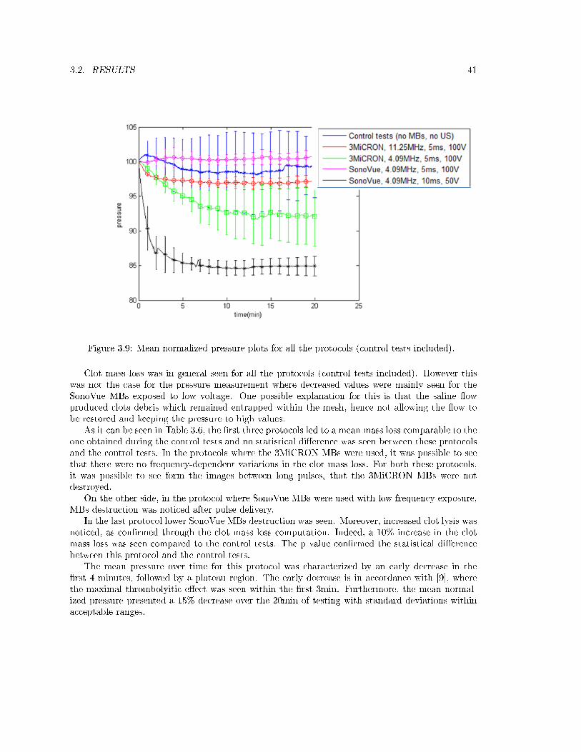
The two types of MBs were diluted in saline (NaCl) in order to have a concentration of 2x106MBs/mlas stated in [9]. Afterwards, MBs and NaCl solution were delivered to the vessel phantom using the50ml syringe and the infusion pump. When the MBs were seen in the clot area (applying B-modeimaging), the sequence of long pulses was started and after 20min the clot mass loss was computed.The upstream pressure was continuously recorded for 20 minutes. The pressure measurements andclot mass loss were compared in order to give an estimation of the thrombolytic e�ciency. Thetime for the tests was chosen in accordance to [9, 27] where it was seen that this time was su�cientfor the detection of the thrombolytic e�ciency.

During the tests, the ultrasound transducer was �xed by a metallic holder and kept in contactwith the phantom surface, which was previously covered with ultrasound gel. The transducer waspositioned longitudinally to the vessel.

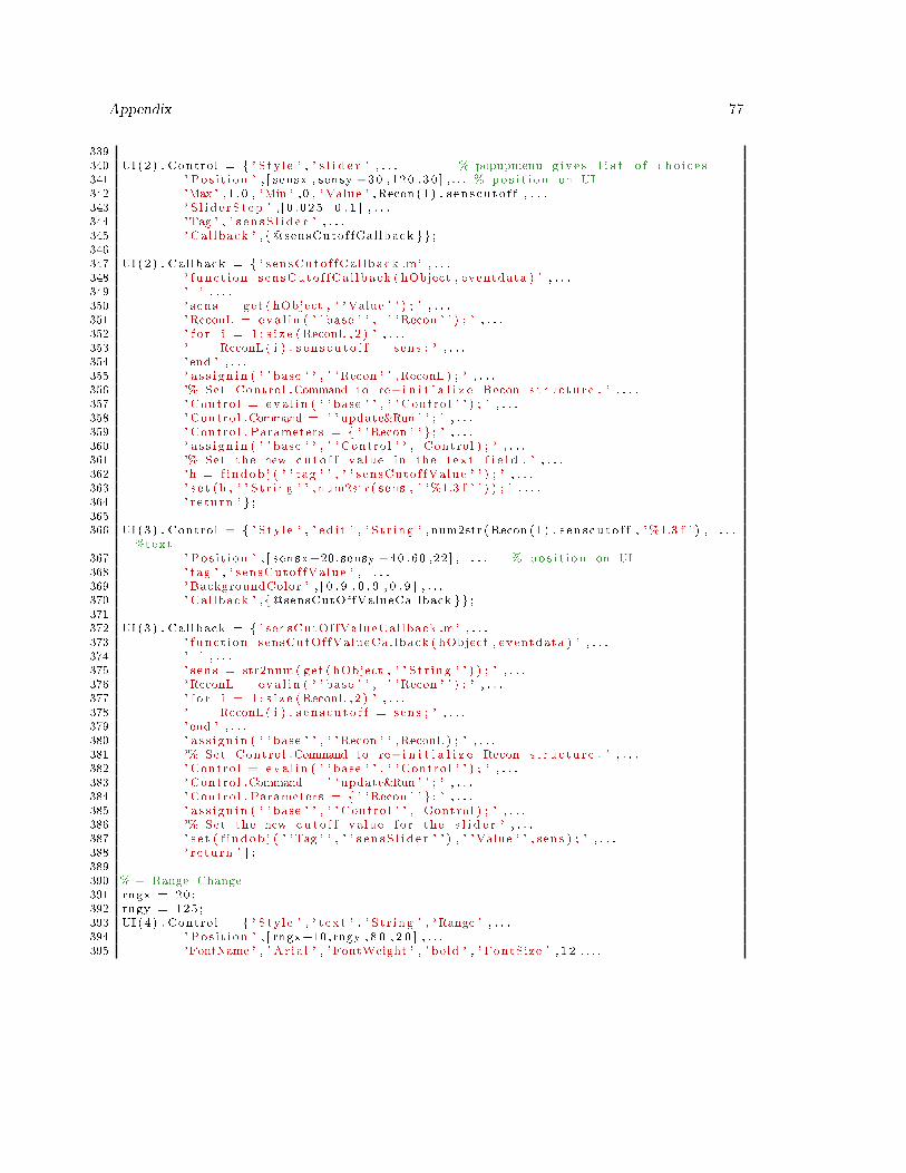
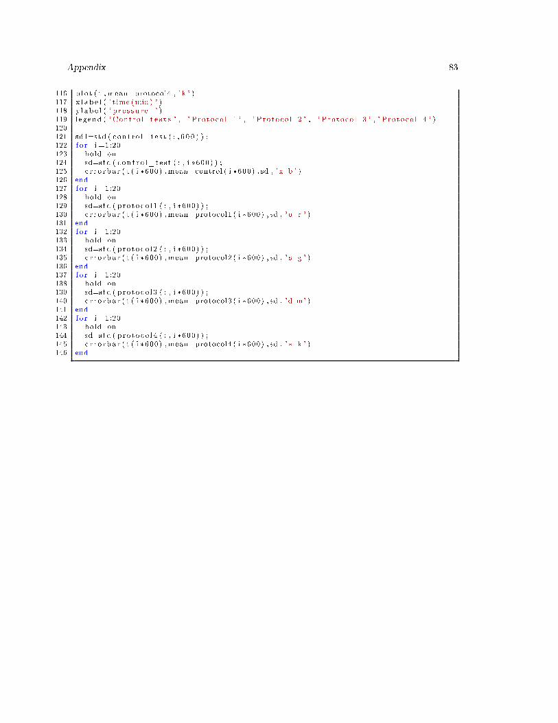
In order to develop the long pulse sequences that were transmitted to the clot area, a codewas programmed using the Verasonics software. The code was written in MatLab (MathWorks,Massachusetts, US) and completely reported in the Appendix.

In the following sections the MBs production, the implemented protocols and the Verasonicsultrasound system architecture are described.

27

28 CHAPTER 3. CLOT LYSIS TESTS WITH ULTRASOUND AND MBS

3.1.1 Production of 3MiCRON MBs

The production of the novel agent was described in [25] and was performed preparing two batchesthat were later added together. For each batch, 200 ml of MilliQ water were mixed with 4g PVA(2%) and heated up to 80 °C. When the mixture reached the desired temperature, 380mg of NalO4

were added and the solution was kept at 80°C for 1 hour continuously agitated with a magneticstirrer. After 1 hour the mixture underwent high shear stirring (8000rpm for 3 hours) in order toselectively split the head-to-head sequence contained in the PVA chains. This stirring was achievedusing an Ultra Turrax (IKA, Germany) at room temperature. The resulting batch was washed seventimes every 24 hours. The obtained MBs have a mean diameter of 3µm and they can be storedin water for months due to their high stability. Before their application, MBs concentration wasassessed using a light microscope and a counting chamber as described in the protocol presented byPretzl and Cerroni in [56]. Brie�y, MBs solution was diluted (1:5) and transferred into the Neubauercounting chamber that has squares with an area of 0.25x0.25mm and a depth of 0.1mm. The images(Figure 3.1) were taken with a transmission microscope (20x objective) and transformed in binarypictures using ImageJ Analysis Software. The binary pictures were than used by the softwarein order to count the particles. Four squares were imaged and analyzed and the mean numberof particles was used for the computation of the concentration. The obtained concentration was109MBs/ml.

Figure 3.1: Image of 3MiCRON MBs with transmission microscope (objective 20x)

3.1.2 Production of SonoVue MBs

The protocol for the SonoVue MBs preparation was �xed by the manufacturer that delivers theSonoVue contrast agent as a kit with a vial containing a lyophilized powder (25mg) and a syringepre�lled with sterile saline solution (5ml). To prepare the MBs the saline solution and the powderwere mixed for 20s. The obtained suspension can be stored for 6 hours and if the MBs accumulateat the upper surface the suspension should be shacked again before the application. The obtainedMBs have a concentration of 1-5x108MBs/ml.

3.1. METHODS 29

3.1.3 Implemented protocols for ultrasound transmission

In order to apply ultrasound with a frequency close to the resonance frequency of the two types ofMBs (1-4MHz for SonoVue and 12MHz for 3MiCRON), the L12-5 50mm transducer transmittingat a frequency equal to 11.25MHz (highest value achievable) and the L7-4 transducer transmittingat 4.09MHz (lowest value achievable) were used. Four protocols for ultrasound transmission weredeveloped and tested. For each of the protocols seven tests were performed. MBs were deliveredafter clot injection and, when they were seen in the clot region, ultrasound exposure was performedfor 20 minutes. Moreover, seven control tests with no ultrasound and no MBs were executed andused as reference. In Table 3.1 the di�erent protocols are summarized.

Table 3.1: The protocols developed and testedMBs

TYPES

TRANSDUCER/FREQUENCY

(MHz)

VOLTAGE

(V)

PULSE

DURATION

(ms)

DISTANCE

TRANSDUC-

ER/CLOT

(mm)

NUMBER

TRANSMIT-

TING

ELEMENTS

3MiCRON L12-5 50mm/11.25 100 5 10 56

3MiCRON L7-4/4.09 100 5 25 40

SonoVue L7-4/4.09 100 5 25 40

SonoVue L7-4/4.09 50 10 25 40

The ultrasound focus was set within the clot region and the long pulses were sent from a subsetof transducers elements in order to cover an area of 10-11mm that included the clot and a smallsurrounding region.

The distance between the transducer and the clot area was approximately 10mm in the �rstprotocol, where the L12-5 50mm transducer was used. In the remaining protocols, since the fre-quency applied was lower, the distance was set equal to 25mm. The highest voltage applied duringthe long pulse delivery was equal to 100V, the highest value achievable, due to safety aspects of thesystem.

Between the long pulses, idle time was set in order to enable the MBs replenishment. Indeed,with a �ow velocity equal to 2mm/s, the time necessary for the MBs replenishment was approxi-mately 6s.

During the exposure of the clots to ultrasound and MBs, no imaging was performed except atone time point to check the e�ective MBs replenishment. This imaging was performed during theidle time between two trains of pulses using the already built-in MatLab script provided with theVerasonic software and opportunely modi�ed for having imaging only during the idle time and notduring the transmission of the long pulses. In this way, in the case of MBs destruction within theclot region during the long pulse delivery, imaging enabled to see if the idle time was su�cient forletting new MBs to reach the area.

For each group of tests the clot mass loss was computed and the mean initial mass and meanmass reduction with the respective standard deviation was calculated. Statistical analysis wasperformed applying the student's t-test in order to compare the mass loss for each protocol withthe control group. Statistical signi�cance was de�ned as p<0.05.

Beside clot mass loss, three pressure measurements for three di�erent tests within each protocolwere considered. The pressure plots were only three due to the di�cult reproducibility of themeasurements caused by the leakages problem.


The pressure measurements of the three considered tests were �ltered using an average �lter.The �ltering was performed averaging 200 data around the output value using the MatLab function�lter. Afterwards, pressure plots were normalized to the �rst value and the mean normalized pressurewas plotted together with standard deviations bars. Normalization of the plots was necessary inorder to allow comparisons due to the fact that slightly di�erent values in the initial clot mass ledto di�erent initial pressure values.

Each long pulse delivered using the Verasonics system consisted in trains of pulses and in Table3.2 their characteristics are summarized for all the protocols. In the next sections the explanationof each pulse sequence will be provided.

Table 3.2: Train of pulses characteristics.PROTOCOL SINGLE PULSE

DURATION(μs)

IDLE TIME(μs)

NUMBEROF PULSES

3MiCRON andhigh frequency

88.18 35.82 40

3MiCRON and lowfrequency

240 7 20

SonoVue and lowfrequency

240 7 20

SonoVue withlonger pulse andlower voltage

240 7 40

3.1.3.1 Control tests: no MBs and no ultrasound application

Control tests were performed delivering saline solution without MBs after clots injection. Ultra-sound was used just for imaging purposes and the long pulses with high voltage were not applied.In order to image the clot area, the L7-4 transducer was used and B-mode images were obtainedusing the already built-in MatLab script provided with the Verasonic software.

3.1.3.2 3MiCRON and high frequency exposure

In this protocol, the 3MiCRON MBs and long ultrasound pulses (5ms), with a frequency equal to11.25MHz and voltage set to 100V, were applied (Table 3.1, �rst row).

The long pulses were sent from the 56 central elements of the L12_5 50mm transducer (Figure3.2). Each element transmitted trains of pulses obtained combining 40 pulses, each with durationof 88.18µs (Table 3.2, �rst row), which is the maximal single pulse duration achievable with theVerasonics architecture and with a frequency equal to 11.25MHz . The idle time between thesepulses had duration of 35.82µs. Therefore, 40 pulses with 88.18µs duration and 35.82µs of idle timeled to a train of pulses with total duration of 5ms. A schematic representation of the ultrasoundpulse sequence is shown in Figure 3.3.

3.1. METHODS 31

Figure 3.2: The ultrasound �eld using the L12-5 50mm transducer.

Figure 3.3: The ultrasound pulse sequence

3.1.3.3 3MiCRON/SonoVue and low frequency exposure

Two protocols were identical with the exception of MBs used. For both the types of MBs thefrequency applied was 4.09MHz and the long pulse had duration of 5ms (Table 3.2, second andthird row). The long pulses were sent from the 40 central elements (Figure 3.4) and they wereobtained combining 20 pulses, each with duration of 240µs, which is the maximal length achievablewith the Verasonics system and with a frequency equal to 4.09MHz (Table 3.2, second and third


rows). The idle time between these pulses had duration of 7µs. Therefore, combination of 20 ofthese pulses led to a train of pulses with duration of 5ms (Figure 3.5).

Figure 3.4: Ultrasound �eld with transducer L7-4.

3.1. METHODS 33

Figure 3.5: The ultrasound pulse sequence

3.1.3.4 SonoVue with longer pulse and lower voltage exposure

In this protocol SonoVue MBs were considered with ultrasound exposure at a frequency of 4.09MHz.The voltage was reduced by 50% and long pulse duration was doubled in comparison to the previousprotocols (Table 3.2, last row).

The long pulses were sent from the 40 central elements and in order to achieve 10ms duration, 40pulses of the same duration and the same idle time as in the previous two protocols were combined(Figure 3.6 and Table 3.2, last row).

Figure 3.6: The ultrasound pulse sequence.


3.1.4 The Verasonics system

The aim of this section is not to provide a complete description of the Verasonics architecture, butonly an overview in order to better understand the developed code. For a detailed explanation ofthe Verasonic system the reader should refer to the Verasonics Sequence Programming Manual.

The Verasonics system is an ultrasound system architecture (Figure 3.7 ) that enables imple-mentation of traditional and new ultrasound sequences. Moreover, it is very �exible in transmitting,receiving and processing ultrasound. The Verasonics architecture allows also the simulation of thesystem using a software simulator running on the host computer. This enables the possibility tocheck the programmed sequence before running it with the probe and the hardware.

Figure 3.7: The Verasonics system (picture taken from the Verasonics brochure)

The Software-based System

The system is programmed generating a collection of objects which are de�ned using a MatLabscript and characterized by speci�c attributes. After executing the script, a MatLab.mat �le isgenerated, which can be loaded into the system by the VSX program (Verasonic Script eXecution).This program performs checks on the script and adds other attributes necessary for the VerasonicsData Acquisition System (VDAS) hardware. At the same time a GUI and a display window aredisplayed. The GUI panel allows the user to change some parameters such as voltage, gain and thedynamic range, while the display window reproduces the image of the region where the ultrasoundwaves are delivered.

In the �nal step the sequence is loaded into the hardware sequencer and executed.

The VDAS Hardware

The VDAS hardware is schematically shown in Figure 3.8 . The front of the available 4 board systemis composed by a scanhead interface with two connectors for plugging the desired transducers. The128 channels of the �rst connector are connected to the 128 A transmitters and the 128 channels ofthe second connector are connected to the 128 B transmitters. The connectors include a system for

3.1. METHODS 35

detecting the presence of the probe and for allowing the execution of the sequence event without it.The acquisition modules are stored inside the chassis and they contain the circuitry for transmittingand receiving the signals for multiple channels. These modules contain also a local memory for thestorage of the received signals before sending them to the host computer. The VDAS hardwarecontains also a Transmit Power Controller module which has the high voltage supplier for thetransmitters. This module allows for high power bursts and extended pulse length.

Figure 3.8: The VDAS hardware (picture taken from the Verasonics Tutorial)

The Objects de�nition

The objects that have to be de�ned in the MatLab script in order to run the sequence can besubdivided in two groups:

1. The System objects: this group of objects is needed in order to de�ne the transducer used,the scanning format and the pixel data region. It also includes the resource object, whichcontains information about the storage bu�ers.

2. The Sequence objects: this set of objects include instructions for the transmission, recep-tion, reconstruction and processing of the ultrasound. Moreover, through the Event object,it is possible to de�ne the events for acquiring one or more frames of data.

Each object is de�ned and described by a set of attributes. For example, some of the Transducerattributes are:

� name: a string containing the scanhead name

� frequency : the center frequency expressed in MHz

� type: linear, curvilinear or 2D

� elementWidth: the element width expressed in wavelength

� spacing : the element spacing in wavelength

� radius: the radius of curvature

For a complete list of the attributes for the transducer and for all the other objects, the readershould refer to the Verasonics Tutorial.


3.1.5 The implemented codes

In order to program the Verasonics system and the transducer for the delivery of long train of pulses,the following objects have to be de�ned in the MatLab code: some initial resource parameters, thetransducer, the storage bu�er, the waveform, the transmission, the time gain controller, the receivingprocess, the control sequence and the list of the events.

For each of the protocols a code was implemented. The objects de�ned in these codes arepresented in the following section. The complete code for each protocol is reported in the Appendix.The distance units in the code are expressed in wavelengths (λ) computed considering the centralfrequency of each transducer (5MHz for the L7-4 and 9MHz for the L12-5 50mm).

3.1.5.1 The Resource.Parameters attribute

The resource.Parameters stores some attributes that are global and required for the con�gurationof the system. These parameters were set equal for all the codes. In the developed sequences theparameters that had to be de�ned were the number of transmit and receive channels (128 for both)and the speed of sound (1540m/s). The simulationMode and fakeScanhead attributes, when setto 1, allowed running the program respectively in simulation mode or without the probe. Theseattributes enabled to check the pulse sequence before running the program with the hardware andthe probe.

3.1.5.2 The Transducer object

For each ultrasound probe used, a Trans object was de�ned. Setting the Trans.name attributeequal to `L12-5 50mm' and to `L7-4' and running the function computeTrans led to the de�nitionof transducers with the characteristics presented in Table 3.3 .

Table 3.3: The transducer attributes.TRANS ATTRIBUTE DESCRIPTION L12-5 50mm L7-4

numelements Number ofelements in thetransducer

256 128

frequency Central frequencyof the transducer

9MHz(λ1=0.17µm)

5MHz(λ2=0.3µm)

spacing The spacingbetween the

elements, includingthe element width

1.14λ1 0.97λ2

maxHighVoltage Maximal voltage(half of the peak to

peak value)

50 50

impedance Compleximpedance at thecentral frequency

45-60i 45-60i

3.1. METHODS 37

3.1.5.3 The Resource object

If imaging is not needed, no storage bu�ers are needed. However the VSX program requires thatat least one storage bu�er is de�ned. For this purpose, for all the protocols, one odd RcvBu�erwas speci�ed for the storage of the data from the local memories on the VDAS modules. However,these data were not further processed. The RcvBu�er contained a number of frames that was setto 1 in order to let the program to run.

3.1.5.4 The TW object

The TW object de�nes the transmit waveform for each transmitter. The type was set to `para-metric' because it had to be generated by the VDAS hardware. The parametric waveform wasdescribed by the four descriptors in the TW.Parameters (A, B, C and D), di�erent for the twotransducers used, and by the extendBL attribute, always set equal to 1. In Table 3.4 the values setfor the two transducers are presented.

Table 3.4: The TW attributes. A value chosen according to Table 3.2.1.1 in the Verasonics SequenceProgramming Manual.

TW ATTRIBUTE DESCRIPTION L12-5 50mm L7-4

Parameters

A waveformfrequency

expressed by thenumber of transmitclock periods in a

half cycle

8 (11.25MHz) 22 (4.09MHz)

B the duty cycleperiod expressedby the number oftransmit clock

periods the positiveor negative drive isactive during thehalf cycle period

3 (37%) 8 (37%)

C the pulse lengthexpressed by thenumbers of half

cycle periods (0-31)

31 (1.38µs) 31 (3.7µs)

D the polarity: 1(�rst transmissionpositive) or -1

(�rst transmissionnegative)

1 1

extendedBL If set to 1 lead tothe multiplicationof the C value by

64

1 1


3.1.5.5 The TX object

This object de�nes all the aspects about the transmit waveform and the timing for each of theactive element in the transducer aperture. The attribute that were set equally in all the codeswere the waveform, the origin and the transmitter delay. For each of the active transmitter theused waveform was the one de�ned in the TW object. For this reason the waveform attributeof the TX object was set to 1. In this way, all the transmit elements were characterized by thesame waveform. The origin point, which is the point on the transducer that the beam appears tooriginate from, was de�ned setting the x, y, z coordinates equal to 0. The delay for each activetransmitter was computed calling the function computeTXDelays(TX(1)) that is already availablewithin the Verasonic software.

The attributes that were set di�erently for the two transducers were the focus value, the Apodarray for the selection of the active transmitters and the transducer aperture. These values arereported in Table 3.5.

TX ATTRIBUTE DESCRIPTION L12-5 50mm L7-4

focus Focal distance inwavelengths

60λ1 85λ2

aperture Selects asub-aperture of thefull array aperture

65 (becausetransmit

channels=128,while

Trans.numelements= 256)

Not needed

Apod Array with 0(transmitter on)and 1 (transmitter

o�) values

56 central valuesequal to 1. The

other 72 equal to 0.

40 central valuesequal to 1. The

other 88 equal to 0.

Table 3.5: The TX attribute

3.1.5.6 The TPC object

The Verasonics Transmit Power Controller is an object that provides for rapid changes in highvoltage output, allowing the use of di�erent power levels for di�erent modes of acquisition. Eachpower level can have its own set of unique attributes, including speci�cation of transmit drivevoltage level, and maximum power output. The collection of attributes for a given power level isreferred to as a pro�le, and up to four pro�les are supported in the current TPC �rmware, with a�fth available as a �high power� option. The TPC pro�le 5 allows use of the system at very hightransmit power levels. In particular, the "Extended Burst Option" utilizes a dedicated internalpower supply with 48 Watt capacity to power the HIFU transmit bursts. A large energy storagecapacitor provided within the system allows transmit for short bursts at much higher power levels,provided that enough time is allowed between bursts to recharge the capacitor from the internalsupply. The amount of transmit power available is highly dependent on the transmit burst duration,the number of active transmit channels, and the load impedance presented by the transducer to thesystem. The pro�le 5, when de�ned in the code, enabled the use of the extendBL attribute, whichwas necessary for having longer pulses.

3.1. METHODS 39

For the protocols where 100V were applied, the maximal voltage was set to 50V, meaning apeak to peak value of 100V, de�ning the maxHighVoltage and highVoltageLimit of pro�le 5 equalto 50.

3.1.5.7 The TGC object

When imaging is not needed, the Time Gain Compensation is not necessary. However, the VerasonicVDAS requires the de�nition of at least one TGC object that has to be referenced in the Receiveobject (see next paragraph). In the developed script the TGC object used was the same found inall the scripts already provided within the Verasonic software.

3.1.5.8 The Receive object

This object de�nes all the characteristics of the receive phase of an acquisition event. Therefore,when imaging is not required, this object is not needed. However, as the RcvBu�er had to be de�nedalso the associate Receive structure had to be set in order to run the VDAS program. Therefore,the MatLab code was taken from an already built in script just to de�ne a simple Receive objectand let the VDAS to run.

3.1.5.9 The Sequence Control object and the Event object

The SeqControl object provides the �ow control of the Events which are de�ned immediately after.For all the codes the �rst Event that had to be de�ned was the one that enabled to switch to

pro�le 5. The associated SeqControl commands used were `setTPCPro�le' with the argument setto 5 and the `noop' command set to 8ms. The �rst command enables the transmission using thehigh power pro�le 5, while the second set 8ms for ensuring enough time to change to pro�le 5, dueto the not immediate switching.

The Events for the delivery of the long train of pulses were slightly di�erent for the di�erentcodes depending on the number of single pulses that were sent. For having 5ms train of pulses at11.25MHz and 10ms at 4.09MHz, 40 events were required. on the other hand, for having 5ms trainof pulses at 4.09MHz, 20 events were required.

After the train of pulses was sent, 6s of idle time were set for MBs replenishment. After thisperiod of time the sequence was repeated from the second event (the one immediately after thesetting of the pro�le 5) using the SeqControl command `jump' . When the command `jump' wascalled, an unconditional branch was performed to the event indicated in the argument which in thespeci�c case was the number 2. In the end, the last events after the `jump' command were required inorder to run the VDAS program. Indeed, this program required that at least one `transferToHost 'command was set, generating a command needed by the VSX. The `transferToHost ' commandrequired that at least one receiving event was present. In order to satisfy this request a shamreceiving event using the fake Receive object and RcvBu�er was set.


3.2 Results

Table 3.6 summarizes the initial mean weight and the mean mass loss, with the corresponding pvalue, for the control tests and the four protocols. Moreover, in Figure 3.9 the change in upstreampressure over exposure time is presented.

Table 3.6: Initial mean weight and mean mass loss for each protocol (control tests included). NS=not signi�cant, n=number of clots tested.

PROTOCOL INITIALMEAN

WEIGHT±SD (g)

MEANMASS LOSS± SD (%)

p-value

Control tests(n=7)

0.064 ± 0.007 38 ± 9.6 -

3MiCRON andhigh frequency

(n=7)

0.054 ±0.01 37 ± 9.7 NS

3MiCRON andlow frequency

(n=7)

0.063 ± 0.01 37.2 ± 5.4 NS

SonoVue andlow frequency

(n=7)

0.051 ± 0.01 35.8 ± 6.3 NS

SonoVue withlonger pulse andlower voltage

(n=7)

0.063 ± 0.01 49 ± 7.9 0.025

3.2. RESULTS 41

Figure 3.9: Mean normalized pressure plots for all the protocols (control tests included).

Clot mass loss was in general seen for all the protocols (control tests included). However thiswas not the case for the pressure measurement where decreased values were mainly seen for theSonoVue MBs exposed to low voltage. One possible explanation for this is that the saline �owproduced clots debris which remained entrapped within the mesh, hence not allowing the �ow tobe restored and keeping the pressure to high values.

As it can be seen in Table 3.6, the �rst three protocols led to a mean mass loss comparable to theone obtained during the control tests and no statistical di�erence was seen between these protocolsand the control tests. In the protocols where the 3MiCRON MBs were used, it was possible to seethat there were no frequency-dependent variations in the clot mass loss. For both these protocols,it was possible to see form the images between long pulses, that the 3MiCRON MBs were notdestroyed.

On the other side, in the protocol where SonoVue MBs were used with low frequency exposure,MBs destruction was noticed after pulse delivery.

In the last protocol lower SonoVue MBs destruction was seen. Moreover, increased clot lysis wasnoticed, as con�rmed through the clot mass loss computation. Indeed, a 10% increase in the clotmass loss was seen compared to the control tests. The p value con�rmed the statistical di�erencebetween this protocol and the control tests.

The mean pressure over time for this protocol was characterized by an early decrease in the�rst 4 minutes, followed by a plateau region. The early decrease is in accordance with [9], wherethe maximal thrombolyitic e�ect was seen within the �rst 3min. Furthermore, the mean normal-ized pressure presented a 15% decrease over the 20min of testing with standard deviations withinacceptable ranges.


Chapter 4

Discussion and Conclusions

4.1 Design and optimization of the in-vitro set-up

As it can be seen from the results obtained during the validation process, the optimal set-up wasnot easy to achieve.

Several problems arose during the realization and the main ones were related to leakage problemsand air bubble formation.

The air bubbles formation was e�ectively solved switching from the peristaltic pump to theinfusion pump. Air bubbles led to the presence of some random peaks in the pressure patterns.After the �ush and during the continuous infusion the pressure curves were more regular and norandom peaks were present. Therefore, air bubbles formation was avoided. The solution chosen forthe �nal set-up was to use the continuous infusion pump because, beside eliminating the problemof the air bubbles formation, it led to a more realistic set-up.

The leakage problems a�ected the pressure measurements, which were not always reliable as theclot mass computation before and after each test.

The �nal in-vitro set-up presented several aspects similar to the physiological situation of oc-cluded coronary arteries. The vessel lumen was 4mm in size, comparable to the dimension of theleft anterior descending coronary artery. Moreover, the 40µm pore mesh reproduced the microcir-culation and the �ow velocity was 2mm/s, similar to the real situation value. Lastly, the materialof the phantom had acoustic properties comparable with the soft tissues ones.

On the other side, the distance between the clot region and the ultrasound transducer was notcomparable to the real distance between the probe and the coronary arteries. Moreover, in thereal situation the presence of the ribs and other body structures that can attenuate and scatter theultrasound waves makes the application of linear transducers not possible. Another limitation ofthe in-vitro set-up was the continuous �ow delivery, which is not present in the real situation wherethe �ow is pulsatile. Moreover, the implemented set-up did not allow estimation of the clot debrisstuck in the mesh.

43

44 CHAPTER 4. DISCUSSION AND CONCLUSIONS

4.2 Test of the in-vitro set-up with ultrasound and MBs

In general, using the Verasonics system, several limitations in the coding and implementation ofdi�erent combinations of ultrasound parameters were found. This was due to the fact that the entiresystem had power limitations and hardware constraints that did not allow realization of continuouslong pulses. Another general limitation for all the protocols (control tests included) was the lownumber of tests performed. Higher number of tests will enable more reliable statistics.

4.2.1 Control tests

The control tests, with no application of ultrasound and MBs led to a mean mass loss equal to 38± 9.6 %.

In another study [30], were ultrasound e�ciency was studied in a set-up were no �ow was present,the control test (20min of clot immersion in saline solution) led to a clot reduction of 29 ± 11%.The weighing procedure was similar to the one presented in this work. The higher clot mass lossfound in the present project was probably due to the �ow delivery, which may be able to furtherreduce the clot size. Another aspect to consider is that the clots produced in [30] are obtainedletting human blood to coagulate spontaneously after being drawn. The di�erent methods for clotsproduction may be another reason for di�erent values in clot mass loss. Moreover, the mean initialweight of the clots produced within this project was much lower than the mean weight of the clotsfound in [30], because of the 4mm diameter vessel. Indeed, the mean initial mass of the 3-4mmclots computed considering all the tests of all the protocols (control tests included) was 0.057 ±

0.01 g. In [30] that value was equal to 0.498 ± 0.073 with a size of approximately 1cm. The smalldimension of the clots used in the present project led to a more di�cult mass loss computation.

Comparing the results obtained computing the clots mass loss and the pressure measurementsduring the control tests it seemed that the pressure sensor was not able to detect the 38% massloss. Therefore, potential clot debris was probably bigger in size than the mesh pores (40µm),hence remaining stuck in the mesh and keeping the pressure to high values. In a real physiologicalsituation this will lead to the occlusion of the microcirculation (approximately 40µm in size). Afurther study with a microscope, in order to analyze the mesh, may con�rm this possibility.

4.2.2 3MiCRON with high and low frequency exposure

The frequency value of 4.09MHz, applied delivering 3MiCRON MBs was lower than the resonancefrequency. On the other side, the highest frequency applied was closer to the resonance frequency,but still not equal due to the transducer used and the Verasonics hardware limitation. The enhance-ment of the non-linear oscillation of 3MiCRON MBs is maximal when the resonance frequency isapplied. In the tests performed the MBs might have passed the clot and the mesh without any e�ectwhen delivering ultrasound at 4.09MHz and also the highest value may has not been su�cient. Ifnon-linear oscillation is considered as one possible reason for clot lysis, in the considered tests theoscillation may has not been enhanced su�ciently in order to increase the clot reduction.

In [30], application of ultrasound without MBs led to decreasing thrombolysis e�ciency withincreasing frequency. Considering this result, a limitation of the 3MiCRON MBs might be the needof very high frequencies in order to trigger an oscillation that can improve the clot lysis.

For both the protocols where 3MiCRON MBs were applied, the intensity delivered to the clotarea was reduced by 43% of the transmitted value. Therefore, of the 100V sent from the transducers,57V reached the clot. The voltage is the only indication of the ultrasound wave amplitude. No

4.2. TEST OF THE IN-VITRO SET-UP WITH ULTRASOUND AND MBS 45

information about the intensity or pressure was available due to the fact that the Verasonics systemenabled only the setting of the voltage. Thus, the mechanical index could not be computed andthe comparison with other studies mentioned in the background section was di�cult. The imagesafter the long trains of pulses did not show regions were no bubbles were present and one possibleexplanation of this could be that the intensity was not enough high to disrupt the MBs. 3MiCRONMBs have much sti�er shell than other lipid-encapsulated MBs, hence they may require very highvalues of intensity, not achievable with the L7-4 and L12-5 50mm transducers and the Verasonicssystem.

In [9], a peak-to-peak acoustic pressure of 1.5MPa led to high thrombolytic e�ciency in the�rst 5min of testing with 5ms pulse duration. In detail, the pressure decreased by 75% over 20minof testing. In the present work no pressure decrease was found, thus the value of 57V in the clotregion might not be su�cient for triggering the cavitation process or MBs oscillation. Moreover, in[34] it was seen that cavitation threshold increased with increasing frequencies values. Therefore,if the cavitation is supposed to be one of the main mechanisms of clot lysis, in the present studythe threshold could have been greatly increased applying a frequency equal to 11.25MHz.

The ultrasound train of pulse with duration of 5ms was chosen in accordance to the value usedin [9]. However, in [9] the pulse length was delivered form a single element transducer and the 5mspulse was continuous. In the present work the 5ms pulse was composed by several shorter pulseswith small idle times in between. More in detail, using the L12-5 50mm transducer, the longestpulse achievable with 11.25MHz had a duration of 88.18µs, while the L7-4 transmitting at 4.09MHzenabled pulses with maximal duration of 240µs . Thus, in order to obtain a longer pulse, several ofthese short pulses were combined. The idle time in between was the lowest achievable and smallervalues were not possible due to power limitations. Moreover, each pulse had a duty cycle equal to37%. Low values of duty cycle led to irregular waveforms, thus the �nal ultrasound wave did nothave a regular sinusoidal shape with alternating phases of compression and rarefaction.

Due to several power limitation of the system, good compromise between voltage, pulse duration,duty cycle and idle time between pulses had to be found. In order to transmit at 100V, the trainof 88.18µs and of 240µs pulses could not be longer than 5ms. All these limitation in pulse lengthmay a�ect the ultrasound e�ciency in clot lysis and ultrasound interaction with MBs.

4.2.3 SonoVue and low frequency exposure

For the SonoVue MBs it was seen that the pulse burst the bubbles, thus creating a dark area withinthe �ow where almost no bubbles were present. This result is in accordance to previous knowledge,namely that SonoVue bubbles are easier to break compared to the 3MiCORN MBs, which remainedintact when the same ultrasound pulse was delivered.

As seen in the results, this protocol led the conclusion that no improvement in clot lysis wasseen compared to the control tests. One possible explanation of this result is that the 100V pulseswere able to destroy the SonoVue bubbles without triggering any process of clot lysis. As stated inthe Background, several studies found that inertial cavitation (generated when MBs are disrupted)was less e�ective in clot lysis compared with stable cavitation. Stable cavitation was probably notpossible for SonoVue MBs due to their disruption. This could have led to ine�ective clot reduction.

The frequency applied, 4.09MHz was almost in the range of the resonance frequencies forSonoVue (1-4MHz), but the disruption of the bubbles did not allow evaluation of the e�ects ofMBs oscillation.


4.2.4 SonoVue with longer pulse and lower voltage exposure

According to the results obtained in the previous protocol, a new pulse sequence was developedfor the ultrasound application with SonoVue MBs. The lower voltage was set in order to reducethe bubble destruction which was still present but with lower severity. Furthermore, reducing thevoltage, it was possible to program a train of pulses with longer duration (10ms). Longer pulseswere implemented because they were seen e�ective in clot lysis in several studies. In [9], �ve pulseswith increased duration (from 0.1ms to 5ms) were compared, resulting in highest thrombolyitice�ciency with 5ms duration. Moreover, also in [30] it was seen that thrombolysis e�ciency (%)increased with pulse duration.

As seen in the results, the implemented pulse sequence, in conjunction with SonoVue MBs wasable to improve the clot lysis. This may be due to the fact that lower voltage reduced the MBsdestruction, while the longer pulse duration enabled the enhancement of MBs interaction with theclot. The MBs that were not destroyed were triggered with a pulse which, with longer duration andwith a frequency within the range of the resonance frequency for the SonoVue, could have improvedthe MBs oscillation. Furthermore, the MBs oscillation could have enhanced the cavitation withinthe clot area, increasing the clot lysis.

4.3 Conclusion

In the present work, a set-up for sonothrombosis was designed and tested.

The set-up presented several aspects that enabled its comparison with the physiological situationof coronary arteries occlusion, allowing testing of clot lysis with ultrasound exposure in conjunctionwith MBs. However, the set-up had also several limitations and two main problems were found: airbubbles formation within the �ow and leakages phenomena. The �rst one was completely solved,while the leakage was only reduced.

The obtained set-up and the implemented ultrasound sequences were able to allow a �rst studyof the sonothrombolysis with 3MiCRON and SonoVue MBs. From the developed protocols it wasseen that 10ms long pulses, delivered at 50V in conjunction with SonoVue MBs, were able toimprove the clot lysis by 10% compared to the control tests and to the tests where the 3MiCRONMBs were used.

4.4 Future work

The set-up has to be further optimized in order to eliminate the leakage problem and to obtain morereliable pressure measurements. Di�erent phantom materials and geometries should be consideredand tested in order to address these problems. Furthermore, the e�ciency of the clot lysis shouldbe computed considering also the clot debris stuck in the 40µm pore mesh. Developing a methodfor analyzing the material entrapped in the mesh, it will be possible to see if the reason of notvarying pressure over 20min was due to clot debris bigger in size than the mesh pores.

The programmed ultrasound sequences have to be further modi�ed and tested in order toevaluate possible e�ects in clot lysis with di�erent combination of ultrasound parameters. Di�erentpulse lengths, voltages and frequencies should be tested in order to �nd the right combinationfor higher thrombolytic e�ects when delivering 3MiCRON or SonoVue MBs. In addition, theapplication of di�erent transducers should be considered. For example, using a single-element

4.4. FUTURE WORK 47

transducer it will be possible to have fewer limitations compared with the programmable system,although the setting will be less realistic when compared to the clinical one.


Bibliography

[1] Media centre, WHO, The 10 leading causes of death by broad income group (2008), UpdatedJune 2011, http://who.int/mediacentre/factsheets/fs310/en/ (accessed 07/06/2013).

[2] Walter F. Boron, Emile L. Boulpaep, �Special circulation� in Medical Physiology, UpdatedEdition, Philadelphia: Elsevier Saunders 2005, ch 23, 562-565

[3] Lippi G et al., �Arterial thrombus formation in cardiovascular disease�, Nat. Rev Cardiol.,2011; 8(9); 502-512

[4] Robert S. Shwartz, �Microemboli and microvascular obstruction in acute coronary thrombosisand sudden coronary death�, Journal of the American College of Cardiology, 2009; Vol 53; No23.

[5] Aldons J. Lusis, �Atherosclerosis�, Nature,2000, vol 407; 233-241.

[6] Legein et al., �In�ammation and immune system interactions in atherosclerosis�, Cell. Mol.Life Sci., 2013, DOI 10.1007/S00018-013-1289-1.

[7] Linco� AM, Topol EJ, �Illusion of reperfusion.Does anyone achieve optimal reperfusion duringacute myocardial infarction?�, Circulation, 1993; 88; 1361-1374

[8] Ito H., �No re�ow phenomenon and prognosis in patients with acute myocardial infarction�,Nat. Clin. Pract. Cardiovasc. Med, 2006; 3; 499-506.

[9] Leeman E. et al., �E�ective of acoustic conditions on microbubble-mediated microvascularsonothrombolysis�, Ultrasound in Med and Biol, 2012; Vol 38; 9; 1589-1598

[10] Janice L. Hinkle, �Acute Ischemic Stroke review�, J Neurosci. Nurs., 2007; 39(5); 285-293, 310.

[11] Muir et al, �Imaging of acute stroke�, Lancet Neurology, 2006; 5; 744�768.

[12] Wolf-Dieter Heiss, �Systemic rtPA in Patients with Acute Ischemic Stroke�, Max-Planck-Institut für neurologische Forschung, Köln, Germany [Online]. Available:http://www.fac.org.ar/scvc/llave/stroke/heiss/heissi.htm (accessed 15-02-2013)

[13] Marler JR, �Tissue plasminogen activator for acute ischemic stroke�, N Engl J Med; 1995; 333;1581-1587

[14] Blakeley JO, Llinas RH. �Thrombolytic therapy for acute ischemic stroke�. J.Neurol.Sci.2007;261:55-62.

49

50 BIBLIOGRAPHY

[15] H.P. Adams et al., �Guidelines for Thrombolytic Therapy for Acute Stroke: A Supplement tothe Guidelines for the Management of Patients With Acute Ischemic Stroke A Statement forHealthcare Professionals From a Special Writing Group of the Stroke Council, American HeartAssociation� Stroke; a journal of cerebral circulation, 1996; 27; 1711-8.

[16] Robert J. Siegel, Huai Luo, �Ultrasound thrombolysis�, Ultrasonics,2008; 48; 312-320

[17] Denise E et al., �Advancements in Catheter-Directed Ultrasound-Accelerated thrombolysis�, JEndvasc Ther, 2011; 18; 418-434

[18] Hirsh J et al., Executive summary: American College of Chest Physicians evidence-basedclinical practice guidelines (8th edition), Chest. ,2008; 133(6 SUPPL. 6); 110S-112S

[19] Hoskins P.R. et al., �Physiscs�, in Diagnostic Ultrasound-Physics and equipment, London, UK,GMM, 2003, ch 1, 7-22.

[20] Ultrasound - Technology INformation Portal, http://www.us-tip.com/serv1.php?type=db, lastupdate 22/04/2013 (accessed 07/06/2013)

[21] Greis, �Technology overview: SonoVue (Bracco, Milan)�, Eur. Rad. Suppl, 2004;14[Suppl 8];11-15.

[22] Shengping Qin et al.,�Ultrasound contrast microbubbles in imaging and therapy: physis-cal principles and engineering� Phys Med Biol, 2009; 54(6): R27. DOI:10.1088/0031-9155/54/6/R01.

[23] Villanueva FS et al, �Targeted ultrasound imaging using microbubbles�, Cardiol. Clin., 2004;22(2); 283-98.

[24] Streeter Jason E. et al., �Improving sensitivity in ultrasound molecular imaging by tailoringcontrast agent size distribution: in vivo studies�, Mol Imaging, 2010; 9(2); 87-95.

[25] Cavalieri et al., �Stable Polymeric Microballoons as Multifunctional Device for BiomedicalUses: Synthesis and Characterization�, Langmuir, 2005;21; 8758-8764.

[26] Kathryn E. Hitchcock and Christy K. Holland, �Ultrasound-Assisted Thrombolysis for StrokeTherapy�, Stroke, 2010;41; S50-S53.

[27] Francis CW et al., �Ultrasound accelerates transport of recombinant tissue plasminogen acti-vator into clots� Ultrasound Med Biol., 1995; 21; 419-424.

[28] Saguchi T et al., �E�ective and safe conditions of low frequency transcranial ultrasonic throm-bolysis for acute ischemic stroke. Neurologica and histologic evaluation in a rat middle cerebralartery stroke model�, Stroke, 2008; 39;1007-1011.

[29] Tachibana K, Tachibana S., �Albumin microbubble echo-contrast material as an enhancer forultrasound accelerated thrombolysis�, Circulation, 1995;92;1148-50.

[30] Schafer et al., �In�uence of Ultrasound operating parameters on ultrasound-induced thrombol-ysis in vitro�, Ultrasound in Med. And Biol, 2005; vol 31, No 6; 841-847.

BIBLIOGRAPHY 51

[31] Rosenschein U et al., �Study of the mechanism of ultrasound angioplasty from human thrombiand bovine aorta� Am. J. Cardiol.,1994; 74; 1263-1266.

[32] Datta et al., �Correlation of cavitation with ultrasound enhancement of thrombolysis�, Ultra-sound Med Biol, 2006;32(8); 1257-1267.

[33] Collis et al., � Cavitation microstreaming and stress �elds created by microbubbles�, Ultrason-ics, 2010;50; 273-279.

[34] Deng et al., �In vitro measurements of inertial cavitation thresholds in human blood�, Ultra-sound Med BIol, 1997; 23; 619-624.

[35] Borelli et al, �In�uences of Microbubble Diameter and Ultrasonic Parameters on in VitroSonothrombolysis E�cacy�, J Vasc Interv Radiol, 2012; 23; 1677-1684.

[36] Stefan Pfa�enberger et al., �Ultrasound thrombolysis�, Thromb Haemost, 2005;94; 26-36.

[37] Tachibana K., Tachibana S., �Enhancement of �brinolysis with ultrasound energy�, J VascInterv Radiol, 1992; 3; 299-303.

[38] Tachibana K., Tachibana S., �Prototype therapeutic ultrasound emitting catheter for acceler-ating thrombolysis�, J Ultrasound Med, 1997; 16; 529-35.

[39] Lynn JG et al., �A new method for the generation and use of focused ultrasound in experimentalbiology�, J Gen Physiol.,1942; 28; 179-193.

[40] Rosenschein et al., �Ultrasound Imaging-Guided Noninvasive Ultrasound Thrombolysis: Pre-clinical Results�, Circulation, 2000; 102; 238-245.

[41] Frenkel et al., �Pulsed High-Intensity Focused ultrasound Enhances Thrombolysis in an in-vitromodel�, Radiology, 2006;239(1);86-93.

[42] Pfa�enberger et al., �Can a Commercial Diagnostic Ultrasound Device Accelerate Thrombol-ysis?: An in Vitro Skull Model�, Stroke, 2005; 36; 124-128.

[43] Xie et al., �Treatment of Acute Intravascular Thrombi With Diagnostic Ultrasound and Intra-venous Microbubbles�, JACC Cardiovasc Imaging, 2009; 2(4); 511-8.

[44] Xie et al., �Diagnostic Ultrasound Combined with Glycoprotein 2b/3a Targeted MicrobubblesImprove Microvascular Recovery Following Acute Coronary Thrombotic Occlusions�, Circula-tion, 2009; 119(10); 1378-1385.

[45] Kutty et al., �Microbubble Mediated Thrombus Dissolution with Diagnostic Ultrasound forthe Threatment of Chronic Venous Thrombi�, PloS One, 2012; 7(12); e51453.

[46] Nesser et al., �Therapeutic Ultrasound in Cardiology�, Herz, 2002; 27; 269-278.

[47] Skoloudik et al., �Safety and e�cacy of the sonographic acceleration of the middle cerebralartery recanalization: results of the pilot thrombotripsy study�, Ultrasound Med Biol, 2008;20;58-63

52 Appendix

[48] Bardon et al., �Safety and e�cacy of sonothrombolysis using bilateral TCD monitor-ing by diagnostic 2MHz probes- a pilot study�, Biomed Pap Med Fac, 2012; 156; DOI:10.5507/BP.2012.064.

[49] Rubiera et al., �Safety and E�cacy of Ultrasound-Enhanced Thrombolysis: A ComprehensiveReview and Meta-Analysis of Randomized and Nonrandomized Studies�, Stroke, 2010;41; 280-287.

[50] Alexandrov et al., �A Pilot Randomized Clinical Safety Study of Sonothrombolysis Augumen-tation With Ultrasound-Activated Per�utre-Lipid Microspheres for Acute Ischemic Stroke�,Stroke, 2008;39(5); 1464-1469.

[51] Parikh et al., �Ultrasound-accelerated Thrombolysis for the treatment of Deep Vein Thrombo-sis: Initial Clinical Experience�, J Vasc Interv Radiol, 2008; 19; 521-528.

[52] Moskovitz, �Ultrasound Accelerated Thrombolysis: A Safe and E�ective, Low-dose Throm-bolytic Therapy for Acute Pulmonary Embolism�, Vein, 2012; issue 3 volume 5.

[53] Malin Larsson et al., �Evaluation of the acoustic response of novel polymer-shelled contrastagents using clinical ultrasound systems� , Submitted to Ultrasonics, 2013.

[54] Devcic-Kuhar, �In vitro thrombolysis enhanced by standing and travelling ultrasound wave�elds� Ultrasound in Med. & Biol., 2002;Vol. 28, No. 9, 1181�1187.

[55] Xie et al., �E�ect of Attenuationc and Thrombus Age on the Success of Ultrasound and Mi-crobubble Mediated Thrombus Dissolution�, Ultrasound Med. Biol.,2011, 37(2), 280-288;

[56] Melanie Pretzl and Barbara Cerroni, �Standard protocol: concentration of MB/ml�, 3MiCRONproject, 2010.

Appendix

1 % F i l e name SetUpL12_5_50mmNoImaging1 .m:2 % code f o r Protoco l 13 % frequency : 11 .25MHz4 % pul s e l ength : 5ms5 % max vo l tage : 100V6 % time between t r a i n s o f long pu l s e s= 6 s78 c l e a r a l l910 % Spec i f y system parameters .11 Resource . Parameters . numTransmit = 128 ; % number o f t ransmit channe l s .12 Resource . Parameters . numRcvChannels = 128 ; % number o f r e c e i v e channe l s .13 Resource . Parameters . speedOfSound = 1540 ; % speed o f sound in m/ sec14 Resource . Parameters . simulateMode = 0 ; % 1=s imu la t i on ; 0=run with hardware15 Resource . Parameters . fakeScanhead=1; % 1= run without probe1617 % Spec i f y Trans s t r u c tu r e array .18 Trans . name = 'L12−5 50mm' ; % L12−5 t ransducer i s ' known '19 Trans . f requency = 9 . 0 ; % cente r f requency20 Trans = computeTrans ( Trans ) ; % L12−5 t ransducer i s ' known '21 Trans . maxHighVoltage = 50 ; % s e t a high vo l tage l im i t .22 Trans . impedance = 45−60 i ; % s e t t ransducer impedance .2324 % Spec i f y Media ob j e c t . ' pt1 .m' s c r i p t d e f i n e s array o f po int t a r g e t s .25 pt1 ;26 Media . f unc t i on = 'movePoints ' ;2728 % Spec i f y Resource .29 Resource . RcvBuffer (1 ) . datatype = ' in t16 ' ; % b i t s i z e o f the sample30 Resource . RcvBuffer (1 ) . rowsPerFrame = 4096 ; % s i z e f o r a c q u i s i t i o n s range31 Resource . RcvBuffer (1 ) . colsPerFrame = Resource . Parameters . numRcvChannels ;32 Resource . RcvBuffer (1 ) . numFrames = 1 ; % number o f frames ( not used )3334 % Spec i f y TW st ru c tu r e array .35 TW(1) . type = ' parametr ic ' ; % waveform type36 TW(1) . Parameters = [ 8 , 3 , 3 1 , 1 ] ; % A=11.25 MHz, B =37%, C =1.4us , D= 137 TW(1) . extendBL = 1 ; % i f equal to 1 , C value mu l t i p l i e d by 64 thus C=88.18 us3839 % Spec i f y TX s t ru c tu r e array .40 TX(1) . waveform=1; % same waveform f o r a l l the e lements41 TX(1) . Or ig in = [ 0 . 0 , 0 . 0 , 0 . 0 ] ; % beam o r i g i n42 TX(1) . f o cus =60 ; %focus at 10 mm43 TX(1) . aper ture = 65 ; % tx aper ture s t a r t s at element 65 .44 TX(1) . Apod =[ z e ro s (1 , 36 ) ones (1 , 56 ) z e r o s (1 , 36 ) ] ;% tx from 56 elem

53

54 Appendix

45 TX(1) . Delay= computeTXDelays (TX(1) ) ; % delay f o r each a c t i v e t r an smi t t e r4647 % Spec i f y P r o f i l e 5 .48 TPC(5) . name = ' long pu l s e ' ; % name o f the p r o f i l e49 TPC(5) . maxHighVoltage = 50 ; % max vo l tage f o r the p r o f i l e50 TPC(5) . h ighVoltageLimit =50; % high vo l tage l im i t based on used model5152 % Spec i f y TGC Waveform s t ru c tu r e .53 TGC. Cntr lPts = [500 , 590 , 650 , 710 , 770 , 830 , 890 , 950 ] ; % va lues a l r eady given54 TGC. rangeMax = 185 ; % max depth o f the range55 TGC.Waveform = computeTGCWaveform(TGC) ; % use func t i on a l r eady bu i l t in5657 % Spec i f y Receive s t r u c tu r e ( not used )58 Receive . Apod= ze ro s (1 , Resource . Parameters . numRcvChannels ) ;59 Receive . aper ture =1;60 Receive . startDepth=2;61 Receive . endDepth=185;62 Receive .TGC=1;63 Receive .mode=0;64 Receive . bufnum=1;65 Receive . framenum=1;66 Receive . acqNum=1;67 Receive . samplesPerWave=4;68 Receive . I npu tF i l t e r =[0 .0036 ,0 .0127 ,0 .0066 , −0 .0881 , −0 .2595 ,0 .6494 ] ;6970 % Spec i f y SeqControl s t r u c tu r e ar rays .7172 % jump back to s t a r t .73 SeqControl (1 ) . command = ' jump ' ;74 SeqControl (1 ) . argument = 2 ;75 % Change to P r o f i l e 5 ( long pu l s e )76 SeqControl (2 ) . command = ' setTPCProf i le ' ;77 SeqControl (2 ) . cond i t i on = ' immediate ' ;78 SeqControl (2 ) . argument = 5 ;79 % Set to a l low time f o r p r o f i l e change .80 SeqControl (3 ) . command = ' noop ' ;81 SeqControl (3 ) . argument = 8000 ;% time in us82 % Set time between long pu l s e s .83 SeqControl (4 ) . command = ' timeToNextAcq ' ;84 SeqControl (4 ) . argument = 124 ; % time in us85 % Set 4 s i d l e time (2 s more with SeqControl (7 ) )86 SeqControl (5 ) . command = ' timeToNextAcq ' ;87 SeqControl (5 ) . argument = 4000000; % time in us88 % Set re turn to MatLab89 SeqControl (6 ) . command = ' returnToMatlab ' ;90 % Set 0 .5 s i d l e time ( used f o r having 2 s more a f t e r SeqControl (5 ) )91 SeqControl (7 ) . command = ' noop ' ;92 SeqControl (7 ) . argument = 500000 ; % time in us9394 % nsc i s count o f SeqControl ob j e c t s95 nsc = 8 ;9697 % n i s count o f Events98 n = 1 ;99100 % Event f o r s e t t i n g the p r o f i l e 5101 Event (n) . i n f o = ' s e t TPCProfile ' ;102 Event (n) . tx = 0 ; % no TX

Appendix 55

103 Event (n) . rcv = 0 ; % no Rcv104 Event (n) . recon = 0 ; % no Recon105 Event (n) . p roce s s = 0 ; % no Proce s s ing106 Event (n) . seqContro l = [ 2 , 3 ] ; % SeqControl (2 ) and SeqControl (3 )107 n=n+1;108 % 40 Events f o r 5ms t r a i n o f pu l s e s109 f o r i = 1 : 40110 Event (n) . i n f o = ' long pu l s e ' ;111 Event (n) . tx = 1 ; % use 1 s t TX s t ru c tu r e .112 Event (n) . rcv = 0 ; % no Rcv113 Event (n) . recon = 0 ; % no r e c on s t ru c t i on .114 Event (n) . p roce s s = 0 ; % no pro c e s s i ng115 Event (n) . seqContro l = 4 ; % time between pu l s e s116 n = n+1;117 end118 % Id l e time 4+2=6s and Return to Matlab119 Event (n−1) . seqContro l = [ 5 , 6 ] ;120 f o r t=1:4121 Event (n) . i n f o=' wait ' ;122 Event (n) . tx = 0 ; % no TX123 Event (n) . rcv = 0 ; % no Rcv124 Event (n) . recon = 0 ; % no Recon125 Event (n) . p roce s s = 0 ; % no pro c e s s i ng126 Event (n) . seqContro l = 7 ; % i d l e time127 n=n+1;128 end129 % repeat sequence o f events from second event130 Event (n) . i n f o = 'Jump back to second event ' ;131 Event (n) . tx = 0 ; % no TX132 Event (n) . rcv = 0 ; % no Rcv133 Event (n) . recon = 0 ; % no Recon134 Event (n) . p roce s s = 0 ; % no pro c e s s i ng135 Event (n) . seqContro l = 1 ;% jump command136 n=n+1;137 % sham events f o r VDAS running138 Event (n) . i n f o = ' sham event ' ;139 Event (n) . tx = 1 ; % no TX140 Event (n) . rcv = 1 ; % no Rcv141 Event (n) . recon = 0 ; % no Recon142 Event (n) . p roce s s = 0 ; % no pro c e s s i ng143 Event (n) . seqContro l = 0 ;144 n=n+1;145 Event (n) . i n f o = ' sham event ' ;146 Event (n) . tx = 0 ; % no TX147 Event (n) . rcv = 0 ; % no Rcv148 Event (n) . recon = 0 ; % no Recon149 Event (n) . p roce s s = 0 ; % no pro c e s s i ng150 Event (n) . seqContro l = nsc ;151 SeqControl ( nsc ) . command = ' trans ferToHost ' ;152 nsc=nsc+1;153154 % Save a l l the s t r u c t u r e s to a .mat f i l e .155 save ( 'L12−5_50mmNoImaging1 ' ) ;

56 Appendix

1 % F i l e name SetUpL7_4NoImaging2_3 .m:2 % code f o r Protoco l 2 and f o r Protoco l 33 % frequency : 4 .09MHz4 % pul s e l ength : 5ms5 % max vo l tage : 100V6 % time between t r a i n s o f long pu l s e s= 6 s78 c l e a r a l l910 % Spec i f y system parameters .11 Resource . Parameters . numTransmit = 128 ; % number o f t ransmit channe l s .12 Resource . Parameters . numRcvChannels = 128 ; % number o f r e c e i v e channe l s .13 Resource . Parameters . speedOfSound = 1540 ; % speed o f sound in m/ sec14 Resource . Parameters . simulateMode = 0 ; % 1=s imu la t i on ; 0=run with hardware15 Resource . Parameters . fakeScanhead=1; % 1= run without probe1617 % Spec i f y Trans s t r u c tu r e array .18 Trans . name = 'L7−4 ' ; % L7−4 t ransducer i s ' known '19 Trans = computeTrans ( Trans ) ; % L7−4 t ransducer i s ' known '20 Trans . maxHighVoltage = 50 ; % s e t a high vo l tage l im i t .212223 % only f o r s imu la t i on24 % Spec i f y Media ob j e c t . ' pt1 .m' s c r i p t d e f i n e s array o f po int t a r g e t s .25 pt1 ;26 Media . f unc t i on = 'movePoints ' ;2728 % Spec i f y Resource .29 Resource . RcvBuffer (1 ) . datatype = ' in t16 ' ; % b i t s i z e o f the sample30 Resource . RcvBuffer (1 ) . rowsPerFrame = 4096 ; % s i z e f o r a c q u i s i t i o n s range31 Resource . RcvBuffer (1 ) . colsPerFrame = Resource . Parameters . numRcvChannels ;32 Resource . RcvBuffer (1 ) . numFrames = 1 ; % number o f frames ( not used )3334 % Spec i f y TW st ru c tu r e array .35 TW(1) . type = ' parametr ic ' ; % waveform type36 TW(1) . Parameters = [ 2 2 , 8 , 3 1 , 1 ] ; % A=4.09 MHz, B =37%, C =3.7us , D= 137 TW(1) . extendBL = 1 ; % i f equal to 1 , C value mu l t i p l i e d by 64 thus C=240us3839 % Spec i f y TX s t ru c tu r e array .40 TX(1) . waveform=1; % same waveform f o r a l l the e lements41 TX(1) . Or ig in = [ 0 . 0 , 0 . 0 , 0 . 0 ] ; % beam o r i g i n42 TX(1) . f o cus =85 ; %focus at 25 mm43 TX(1) . Apod =[ z e ro s (1 , 44 ) ones (1 ,40 ) z e r o s (1 , 44 ) ] ;% tx from 40 elem44 TX(1) . Delay= computeTXDelays (TX(1) ) ; % delay f o r each a c t i v e t r an smi t t e r4546 % Spec i f y P r o f i l e 5 .47 TPC(5) . name = ' long pu l s e ' ; % name o f the p r o f i l e48 TPC(5) . maxHighVoltage = 50 ; % max vo l tage f o r the p r o f i l e49 TPC(5) . h ighVoltageLimit =50; % high vo l tage l im i t based on used model5051 % Spec i f y TGC Waveform s t ru c tu r e .52 TGC. Cntr lPts = [500 , 590 , 650 , 710 , 770 , 830 , 890 , 950 ] ; % va lues a l r eady given53 TGC. rangeMax = 185 ; % max depth o f the range54 TGC.Waveform = computeTGCWaveform(TGC) ; % use func t i on a l r eady bu i l t in5556 % Spec i f y Receive s t r u c tu r e ( not used )57 Receive = repmat ( s t r u c t ( . . .

Appendix 57

58 'Apod ' , z e r o s (1 , Resource . Parameters . numRcvChannels ) , . . .59 ' aper ture ' , 1 , . . .60 ' startDepth ' , 2 , . . .61 ' endDepth ' , 185 , . . .62 'TGC' , 1 , . . .63 'mode ' , 0 , . . .64 ' bufnum ' , 1 , . . .65 ' framenum ' , 1 , . . .66 'acqNum ' , 1 , . . .67 ' samplesPerWave ' , 4 , . . . ' I npu tF i l t e r '

, [ 0 . 0036 ,0 . 0127 ,0 . 0066 , −0 .0881 , −0 .2595 ,0 . 6494 ] ) , . . .68 1 , Resource . RcvBuffer (1 ) . numFrames ) ;6970 % Spec i f y SeqControl s t r u c tu r e ar rays .7172 % jump back to s t a r t .73 SeqControl (1 ) . command = ' jump ' ;74 SeqControl (1 ) . argument = 2 ;75 % Change to P r o f i l e 5 ( long pu l s e )76 SeqControl (2 ) . command = ' setTPCProf i le ' ;77 SeqControl (2 ) . cond i t i on = ' immediate ' ;78 SeqControl (2 ) . argument = 5 ;79 % Set to a l low time f o r p r o f i l e change .80 SeqControl (3 ) . command = ' noop ' ;81 SeqControl (3 ) . argument = 8000 ;% time in us82 % Set time between long pu l s e s .83 SeqControl (4 ) . command = ' timeToNextAcq ' ;84 SeqControl (4 ) . argument = 124 ; % time in us85 % Set 4 s i d l e time (2 s more with SeqControl (7 ) )86 SeqControl (5 ) . command = ' timeToNextAcq ' ;87 SeqControl (5 ) . argument = 4000000; % time in us88 % Set re turn to MatLab89 SeqControl (6 ) . command = ' returnToMatlab ' ;90 % Set 0 .5 s i d l e time ( used f o r having 2 s more a f t e r SeqControl (5 ) )91 SeqControl (7 ) . command = ' noop ' ;92 SeqControl (7 ) . argument = 500000 ; % time in us9394 % nsc i s count o f SeqControl ob j e c t s95 nsc = 8 ;9697 % n i s count o f Events98 n = 1 ;99100 % Event f o r s e t t i n g the p r o f i l e 5101 Event (n) . i n f o = ' s e t TPCProfile ' ;102 Event (n) . tx = 0 ; % no TX103 Event (n) . rcv = 0 ; % no Rcv104 Event (n) . recon = 0 ; % no Recon105 Event (n) . p roce s s = 0 ; % no Proce s s ing106 Event (n) . seqContro l = [ 2 , 3 ] ; % SeqControl (2 ) and SeqControl (3 )107 n=n+1;108 % 20 Events f o r 5ms t r a i n o f pu l s e s109 f o r i = 1 : 20110 Event (n) . i n f o = ' long pu l s e ' ;111 Event (n) . tx = 1 ; % use 1 s t TX s t ru c tu r e .112 Event (n) . rcv = 0 ; % no Rcv113 Event (n) . recon = 0 ; % no r e c on s t ru c t i on .114 Event (n) . p roce s s = 0 ; % no pro c e s s i ng

58 Appendix

115 Event (n) . seqContro l = 4 ; % time between pu l s e s116 n = n+1;117 end118 % Id l e time 4+2=6s and Return to Matlab119 Event (n−1) . seqContro l = [ 5 , 6 ] ;120 f o r t=1:4121 Event (n) . i n f o=' wait ' ;122 Event (n) . tx = 0 ; % no TX123 Event (n) . rcv = 0 ; % no Rcv124 Event (n) . recon = 0 ; % no Recon125 Event (n) . p roce s s = 0 ; % no pro c e s s i ng126 Event (n) . seqContro l = 7 ; % i d l e time127 n=n+1;128 end129 % repeat sequence o f events from second event130 Event (n) . i n f o = 'Jump back to second event ' ;131 Event (n) . tx = 0 ; % no TX132 Event (n) . rcv = 0 ; % no Rcv133 Event (n) . recon = 0 ; % no Recon134 Event (n) . p roce s s = 0 ; % no pro c e s s i ng135 Event (n) . seqContro l = 1 ;% jump command136 n=n+1;137 % sham events f o r VDAS running138 Event (n) . i n f o = ' sham event ' ;139 Event (n) . tx = 1 ; % no TX140 Event (n) . rcv = 1 ; % no Rcv141 Event (n) . recon = 0 ; % no Recon142 Event (n) . p roce s s = 0 ; % no pro c e s s i ng143 Event (n) . seqContro l = 0 ;144 n=n+1;145 Event (n) . i n f o = ' sham event ' ;146 Event (n) . tx = 0 ; % no TX147 Event (n) . rcv = 0 ; % no Rcv148 Event (n) . recon = 0 ; % no Recon149 Event (n) . p roce s s = 0 ; % no pro c e s s i ng150 Event (n) . seqContro l = nsc ;151 SeqControl ( nsc ) . command = ' trans ferToHost ' ;152 nsc=nsc+1;153154 % Save a l l the s t r u c t u r e s to a .mat f i l e .155 save ( 'L7_4NoImaging2_3 ' ) ;

Appendix 59

1 % F i l e name SetUpL7_4NoImaging4 .m:2 % code f o r Protoco l 43 % frequency : 4 .09MHz4 % pul s e l ength : 10ms5 % max vo l tage : 50V6 % time between t r a i n s o f long pu l s e s= 6 s78 c l e a r a l l910 % Spec i f y system parameters .11 Resource . Parameters . numTransmit = 128 ; % number o f t ransmit channe l s .12 Resource . Parameters . numRcvChannels = 128 ; % number o f r e c e i v e channe l s .13 Resource . Parameters . speedOfSound = 1540 ; % speed o f sound in m/ sec14 Resource . Parameters . simulateMode = 0 ; % 1=s imu la t i on ; 0=run with hardware15 Resource . Parameters . fakeScanhead=1; % 1= run without probe1617 % Spec i f y Trans s t r u c tu r e array .18 Trans . name = 'L7−4 ' ; % L7−4 t ransducer i s ' known '19 Trans = computeTrans ( Trans ) ; % L7−4 t ransducer i s ' known '20 Trans . maxHighVoltage = 25 ; % s e t a high vo l tage l im i t .212223 % only f o r s imu la t i on24 % Spec i f y Media ob j e c t . ' pt1 .m' s c r i p t d e f i n e s array o f po int t a r g e t s .25 pt1 ;26 Media . f unc t i on = 'movePoints ' ;2728 % Spec i f y Resource .29 Resource . RcvBuffer (1 ) . datatype = ' in t16 ' ; % b i t s i z e o f the sample30 Resource . RcvBuffer (1 ) . rowsPerFrame = 4096 ; % s i z e f o r a c q u i s i t i o n s range31 Resource . RcvBuffer (1 ) . colsPerFrame = Resource . Parameters . numRcvChannels ;32 Resource . RcvBuffer (1 ) . numFrames = 1 ; % number o f frames ( not used )3334 % Spec i f y TW st ru c tu r e array .35 TW(1) . type = ' parametr ic ' ; % waveform type36 TW(1) . Parameters = [ 2 2 , 8 , 3 1 , 1 ] ; % A=4.09 MHz, B =37%, C =3.7us , D= 137 TW(1) . extendBL = 1 ; % i f equal to 1 , C value mu l t i p l i e d by 64 thus C=240us3839 % Spec i f y TX s t ru c tu r e array .40 TX(1) . waveform=1; % same waveform f o r a l l the e lements41 TX(1) . Or ig in = [ 0 . 0 , 0 . 0 , 0 . 0 ] ; % beam o r i g i n42 TX(1) . f o cus =85 ; %focus at 25 mm43 TX(1) . Apod =[ z e ro s (1 , 44 ) ones (1 , 40 ) z e r o s (1 , 44 ) ] ;% tx from 40 elem44 TX(1) . Delay= computeTXDelays (TX(1) ) ; % delay f o r each a c t i v e t r an smi t t e r4546 % Spec i f y P r o f i l e 5 .47 TPC(5) . name = ' long pu l s e ' ; % name o f the p r o f i l e48 TPC(5) . maxHighVoltage = 25 ; % max vo l tage f o r the p r o f i l e49 TPC(5) . h ighVoltageLimit =25; % high vo l tage l im i t based on used model5051 % Spec i f y TGC Waveform s t ru c tu r e .52 TGC. Cntr lPts = [500 , 590 , 650 , 710 , 770 , 830 , 890 , 950 ] ; % va lues a l r eady given53 TGC. rangeMax = 185 ; % max depth o f the range54 TGC.Waveform = computeTGCWaveform(TGC) ; % use func t i on a l r eady bu i l t in5556 % Spec i f y Receive s t r u c tu r e ( not used )57 Receive = repmat ( s t r u c t ( . . .

60 Appendix

58 'Apod ' , z e r o s (1 , Resource . Parameters . numRcvChannels ) , . . .59 ' aper ture ' , 1 , . . .60 ' startDepth ' , 2 , . . .61 ' endDepth ' , 185 , . . .62 'TGC' , 1 , . . .63 'mode ' , 0 , . . .64 ' bufnum ' , 1 , . . .65 ' framenum ' , 1 , . . .66 'acqNum ' , 1 , . . .67 ' samplesPerWave ' , 4 , . . . ' I npu tF i l t e r '

, [ 0 . 0036 ,0 . 0127 ,0 . 0066 , −0 .0881 , −0 .2595 ,0 . 6494 ] ) , . . .68 1 , Resource . RcvBuffer (1 ) . numFrames ) ;6970 % Spec i f y SeqControl s t r u c tu r e ar rays .7172 % jump back to s t a r t .73 SeqControl (1 ) . command = ' jump ' ;74 SeqControl (1 ) . argument = 2 ;75 % Change to P r o f i l e 5 ( long pu l s e )76 SeqControl (2 ) . command = ' setTPCProf i le ' ;77 SeqControl (2 ) . cond i t i on = ' immediate ' ;78 SeqControl (2 ) . argument = 5 ;79 % Set to a l low time f o r p r o f i l e change .80 SeqControl (3 ) . command = ' noop ' ;81 SeqControl (3 ) . argument = 8000 ;% time in us82 % Set time between long pu l s e s .83 SeqControl (4 ) . command = ' timeToNextAcq ' ;84 SeqControl (4 ) . argument = 124 ; % time in us85 % Set 4 s i d l e time (2 s more with SeqControl (7 ) )86 SeqControl (5 ) . command = ' timeToNextAcq ' ;87 SeqControl (5 ) . argument = 4000000; % time in us88 % Set re turn to MatLab89 SeqControl (6 ) . command = ' returnToMatlab ' ;90 % Set 0 .5 s i d l e time ( used f o r having 2 s more a f t e r SeqControl (5 ) )91 SeqControl (7 ) . command = ' noop ' ;92 SeqControl (7 ) . argument = 500000 ; % time in us9394 % nsc i s count o f SeqControl ob j e c t s95 nsc = 8 ;9697 % n i s count o f Events98 n = 1 ;99100 % Event f o r s e t t i n g the p r o f i l e 5101 Event (n) . i n f o = ' s e t TPCProfile ' ;102 Event (n) . tx = 0 ; % no TX103 Event (n) . rcv = 0 ; % no Rcv104 Event (n) . recon = 0 ; % no Recon105 Event (n) . p roce s s = 0 ; % no Proce s s ing106 Event (n) . seqContro l = [ 2 , 3 ] ; % SeqControl (2 ) and SeqControl (3 )107 n=n+1;108 % 40 Events f o r 10ms t r a i n o f pu l s e s109 f o r i = 1 : 40110 Event (n) . i n f o = ' long pu l s e ' ;111 Event (n) . tx = 1 ; % use 1 s t TX s t ru c tu r e .112 Event (n) . rcv = 0 ; % no Rcv113 Event (n) . recon = 0 ; % no r e c on s t ru c t i on .114 Event (n) . p roce s s = 0 ; % no pro c e s s i ng

Appendix 61

115 Event (n) . seqContro l = 4 ; % time between pu l s e s116 n = n+1;117 end118 % Id l e time 4+2=6s and Return to Matlab119 Event (n−1) . seqContro l = [ 5 , 6 ] ;120 f o r t=1:4121 Event (n) . i n f o=' wait ' ;122 Event (n) . tx = 0 ; % no TX123 Event (n) . rcv = 0 ; % no Rcv124 Event (n) . recon = 0 ; % no Recon125 Event (n) . p roce s s = 0 ; % no pro c e s s i ng126 Event (n) . seqContro l = 7 ; % i d l e time127 n=n+1;128 end129 % repeat sequence o f events from second event130 Event (n) . i n f o = 'Jump back to second event ' ;131 Event (n) . tx = 0 ; % no TX132 Event (n) . rcv = 0 ; % no Rcv133 Event (n) . recon = 0 ; % no Recon134 Event (n) . p roce s s = 0 ; % no pro c e s s i ng135 Event (n) . seqContro l = 1 ;% jump command136 n=n+1;137 % sham events f o r VDAS running138 Event (n) . i n f o = ' sham event ' ;139 Event (n) . tx = 1 ; % no TX140 Event (n) . rcv = 1 ; % no Rcv141 Event (n) . recon = 0 ; % no Recon142 Event (n) . p roce s s = 0 ; % no pro c e s s i ng143 Event (n) . seqContro l = 0 ;144 n=n+1;145 Event (n) . i n f o = ' sham event ' ;146 Event (n) . tx = 0 ; % no TX147 Event (n) . rcv = 0 ; % no Rcv148 Event (n) . recon = 0 ; % no Recon149 Event (n) . p roce s s = 0 ; % no pro c e s s i ng150 Event (n) . seqContro l = nsc ;151 SeqControl ( nsc ) . command = ' trans ferToHost ' ;152 nsc=nsc+1;153154 % Save a l l the s t r u c t u r e s to a .mat f i l e .155 save ( ' L7_4NoImaging4 ' ) ;

62 Appendix

1 % F i l e name SetUpL12_5_50mmImaging .m:2 % code f o r sending long pu l s e s with imaging in between3 % adapted from the Verasonic s c r i p t SetUpL12_5_50mmFlash_4B .m4 % LONG PULSES:5 % − f r equency : 11 .25MHz6 % − vo l tage : 100V7 % − pu l s e l ength : 88 .18 us / i d l e time : 35 .82 us8 % − t r a i n o f pu l s e s l ength : 5ms / i d l e time : 6 s9 % IMAGING:10 % − f r equency : 11 .25MHz11 % − vo l tage : 3V12 % − pu l s e l ength 0 .08 us13 % − three ape r tu r e s14 % 128 transmit channe l s are used f o r each o f 3 transmit ape r tu r e s . On rec e i v e , the15 % 128 channe l s are po s i t i on ed as f o l l ow s ( each char r ep r e s en t s 4 e lements ) :16 % IMAGING17 %18 % Element Nos . 1 1 1 219 % 6 8 2 7 9 520 % 1 5 6 9 2 3 621 % Aperture 1 : | | | | | | |22 % t t t t t t t t t t t t t t t t t t t t t t t t t t t t t t t t −−−−−−−−−−−−−−−−−−−−−−−−−−−−−−−−23 % r r r r r r r r r r r r r r r r r r r r r −−−−−−−−−−−−−−−−−−−−−−−−−−−−−−−−−−−−−−−−−−−24 % | | | | | | |25 % Aperture 2 : | | | | | | |26 % −−−−−−−−−−−−−−−−t t t t t t t t t t t t t t t t t t t t t t t t t t t t t t t t −−−−−−−−−−−−−−−−27 % −−−−−−−−−−−−−−−−−−−−−r r r r r r r r r r r r r r r r r r r r r r −−−−−−−−−−−−−−−−−−−−−28 % | | | | | | |29 % Aperture 3 : | | | | | | |30 % −−−−−−−−−−−−−−−−−−−−−−−−−−−−−−−− t t t t t t t t t t t t t t t t t t t t t t t t t t t t t t t t31 % −−−−−−−−−−−−−−−−−−−−−−−−−−−−−−−−−−−−−−−−−−−r r r r r r r r r r r r r r r r r r r r r32 % | | | | | | |33 %34 % The r e c e i v e data from each o f these ape r tu r e s are s to r ed under d i f f e r e n t acqNums

in the35 % Receive bu f f e r . The r e c on s t r u c t i on sums the IQ data from the 3 a q u i s i t i o n s and

computes36 % i n t e n s i t y va lue s to produce the f u l l frame .37 %38 % This v e r s i on does asynchronous a c q u i s i t i o n and pro c e s s i ng .39 %PULSE TRANSMISSION40 % Aperture 1 : | | | | | | |41 % −−−−−−−−−−−−−−−−t t t t t t t t t t t t t t t t t t t t t t t t t t t t t t t t −−−−−−−−−−−−−−−−424344 c l e a r a l l4546 % Spec i f y system parameters .47 Resource . Parameters . numTransmit = 128 ; % number o f t ransmit channe l s .48 Resource . Parameters . numRcvChannels = 128 ; % number o f r e c e i v e channe l s .49 Resource . Parameters . speedOfSound = 1540 ; % s e t speed o f sound in m/ sec50 Resource . Parameters . simulateMode = 0 ;51 Resource . Parameters . fakeScanhead=1;5253 % Spec i f y Trans s t r u c tu r e array .54 Trans . name = 'L12−5 50mm' ;55 Trans . f requency = 9 . 0 ;

Appendix 63

56 Trans = computeTrans ( Trans ) ; % L12−5 t ransducer i s ' known '57 Trans . maxHighVoltage = 50 ;58 Trans . impedance = 45−60 i ;5960 % Spec i f y SFormat s t r u c tu r e array .61 SFormat . t ransducer = 'L12−5 50mm' ;62 SFormat . scanFormat = 'RLIN ' ; % re c tangu l a r l i n e a r array scan63 SFormat . rad iu s = 0 ;64 SFormat . theta = 0 ;65 SFormat . numRays = 1 ; % Flat Focus66 SFormat . FirstRayLoc = [ 0 , 0 , 0 ] ; % x , y , z67 SFormat . rayDelta = 256*Trans . spac ing ; % spac ing in d i s t . between rays68 SFormat . startDepth = 2 ; % Acqu i s i t i on s t a r t depth in wavelength69 SFormat . endDepth = 185 ; % Acqu i s i t i on end depth in wavelength7071 % Spec i f y PData s t r u c tu r e array .72 PData . sFormat = 1 ; % use f i r s t SFormat s t r u c tu r e .73 PData . pdeltaX = 1 . 0 ;74 PData . pdeltaZ = 0 . 5 ;75 PData . S i z e (1 ) = c e i l ( ( SFormat . endDepth−SFormat . startDepth ) /PData . pdeltaZ ) ;76 PData . S i z e (2 ) = c e i l ( ( Trans . numelements*Trans . spac ing ) /PData . pdeltaX ) ;77 PData . S i z e (3 ) = 1 ; % s i n g l e image page78 PData . Or ig in = [−Trans . spac ing *( Trans . numelements−1) /2 ,0 , SFormat . startDepth ] ;7980 % only f o r s imu la t i on81 % Spec i f y Media ob j e c t . ' pt1 .m' s c r i p t d e f i n e s array o f po int t a r g e t s .82 pt1 ;83 Media . f unc t i on = 'movePoints ' ;8485 % Spec i f y Resources .86 Resource . RcvBuffer (1 ) . datatype = ' in t16 ' ;87 Resource . RcvBuffer (1 ) . rowsPerFrame = 4096*3; % th i s s i z e a l l ows f o r 3 acqs ,

maximum range88 Resource . RcvBuffer (1 ) . colsPerFrame = Resource . Parameters . numRcvChannels ;89 Resource . RcvBuffer (1 ) . numFrames = 245 ; % a l l ows 5 s o f imaging90 Resource . I n t e rBu f f e r (1 ) . datatype = ' complex ' ;91 Resource . I n t e rBu f f e r (1 ) . rowsPerFrame = 1024 ; % th i s i s f o r g r e a t e s t depth92 Resource . I n t e rBu f f e r (1 ) . colsPerFrame = PData . S i z e (2 ) ;93 Resource . I n t e rBu f f e r (1 ) . numFrames = 1 ; % one in te rmed ia t e bu f f e r needed .94 Resource . ImageBuffer (1 ) . datatype = ' double ' ;95 Resource . ImageBuffer (1 ) . rowsPerFrame = 1024 ;96 Resource . ImageBuffer (1 ) . colsPerFrame = PData . S i z e (2 ) ;97 Resource . ImageBuffer (1 ) . numFrames = 10 ;98 Resource . DisplayWindow (1) . T i t l e = ' Image Display ' ;99 Resource . DisplayWindow (1) . pde l ta = 0 . 4 5 ;100 Resource . DisplayWindow (1) . Po s i t i on = [250 ,250 , . . . % upper l e f t corner p o s i t i o n101 c e i l (PData . S i z e (2 ) *PData . pdeltaX/Resource . DisplayWindow (1) . pde l ta ) , . . . %

width102 c e i l (PData . S i z e (1 ) *PData . pdeltaZ /Resource . DisplayWindow (1) . pde l ta ) ] ; %

he ight103 Resource . DisplayWindow (1) . ReferencePt = [ PData . Or ig in (1 ) ,PData . Or ig in (3 ) ] ; % 2D

imaging (X,Z plane )104 Resource . DisplayWindow (1) . Colormap = gray (256) ;105106 % Spec i f y Transmit waveform s t ru c tu r e .107 % f o r imaging108 TW(1) . type = ' parametr ic ' ;109 TW(1) . Parameters = [ 8 , 4 , 2 , 1 ] ; % A=11.25MHz, B =50%, C =0.08us , D= 1

64 Appendix

110 % f o r long pu l s e s111 TW(2) . type = ' parametr ic ' ;112 TW(2) . Parameters = [ 8 , 3 , 3 1 , 1 ] ; % A=11.25MHz, B =37%, C =88.18us , D= 1113 TW(2) . extendBL = 1 ;114115 % Spec i f y TX s t ru c tu r e array .116 % imaging117 TX = repmat ( s t r u c t ( ' waveform ' , 1 , . . .118 ' Or ig in ' , [ 0 . 0 , 0 . 0 , 0 . 0 ] , . . .119 ' aper ture ' , 1 , . . .120 'Apod ' , ones (1 , Resource . Parameters . numTransmit ) , . . .121 ' f o cus ' , 0 . 0 , . . .122 ' S tee r ' , [ 0 . 0 , 0 . 0 ] , . . .123 ' Delay ' , z e r o s (1 , Resource . Parameters . numTransmit ) ) , 1 , 4) ;124 TX(2) . aper ture = 65 ; % Use the tx aper ture that s t a r t s at element 65 .125 TX(3) . aper ture = 129 ; % Use the tx aper ture that s t a r t s at element 129 .126 % f o r long pu l s e s127 TX(4) . waveform = 2 ;128 TX(4) . aper ture = 65 ;129 TX(4) . Apod =[ z e ro s (1 , 36 ) ones (1 , 56 ) z e r o s (1 , 36 ) ] ;130 TX(4) . f o cus =60 ; %focus at 10mm131 TX(4) . Delay= computeTXDelays (TX(4) ) ;132133 % Spec i f y TGC Waveform s t ru c tu r e .134 TGC. Cntr lPts = [500 , 590 , 650 , 710 , 770 , 830 , 890 , 950 ] ;135 TGC. rangeMax = SFormat . endDepth ;136 TGC.Waveform = computeTGCWaveform(TGC) ;137138 % Spec i f y TPC s t r u c t u r e s .139 % p r o f i l e 1 f o r imaging140 TPC(1) . name = ' 2D' ;141 TPC(1) . maxHighVoltage = 50 ;142 TPC(1) . h ighVoltageLimit = 50 ;143 % p r o f i l e 5 f o r long pu l s e s144 TPC(5) . name = ' long pu l s e ' ;145 TPC(5) . maxHighVoltage = 50 ;146 TPC(5) . h ighVoltageLimit =50;147148 % Spec i f y Receive s t r u c tu r e ar rays −149 % endDepth − add add i t i ona l a c q u i s i t i o n depth to account f o r some channe l s150 % having l onge r path l eng th s .151 % Inpu tF i l t e r − The same c o e f f i c i e n t s are used f o r a l l channe l s . The152 % c o e f f i c i e n t s below g ive a broad bandwidth bandpass f i l t e r .153 maxAcqLength = sq r t ( SFormat . endDepth^2 + (Trans . numelements*Trans . spac ing ) ^2) −

SFormat . startDepth ;154 wlsPer128 = 128/(4*2) ; % wavelengths in 128 samples f o r 4 samplesPerWave155 Receive = repmat ( s t r u c t ( 'Apod ' , z e r o s (1 , Resource . Parameters . numRcvChannels ) , . . .156 ' aper ture ' , 1 , . . .157 ' startDepth ' , SFormat . startDepth , . . .158 ' endDepth ' , SFormat . startDepth + wlsPer128* c e i l (

maxAcqLength/wlsPer128 ) , . . .159 'TGC' , 1 , . . .160 ' bufnum ' , 1 , . . .161 ' framenum ' , 1 , . . .162 'acqNum ' , 1 , . . .163 ' samplesPerWave ' , 4 , . . .164 'mode ' , 0 , . . .165 ' I npu tF i l t e r '

Appendix 65

, [ 0 . 0036 ,0 . 0127 ,0 . 0066 , −0 .0881 , −0 .2595 ,0 . 6494 ] , . . .166 ' cal lMediaFunc ' , 0) , 1 , 3* ( Resource . RcvBuffer (1 ) . numFrames ) ) ;167168 % − Set event s p e c i f i c Receive a t t r i b u t e s .169 f o r i = 1 : Resource . RcvBuffer (1 ) . numFrames % 3 a c q u i s i t i o n s per frame170 % −− 1 s t s yn th e t i c aper ture a c q u i s i t i o n f o r aper ture 1 .171 Receive (3* i −2) . Apod ( 1 : 8 5 ) = 1 . 0 ;172 Receive (3* i −2) . aper ture = 1 ;173 Receive (3* i −2) . framenum = i ;174 Receive (3* i −2) . acqNum = 1 ;175 Receive (3* i −2) . cal lMediaFunc = 1 ;176 % −− 2nd syn the t i c aper ture a c q u i s i t i o n f o r aper ture 65 .177 Receive (3* i −1) . Apod (22 : 107 ) = 1 . 0 ;178 Receive (3* i −1) . aper ture = 65 ;179 Receive (3* i −1) . framenum = i ;180 Receive (3* i −1) . acqNum = 2 ;181 % −− 3 rd syn the t i c aper ture a c q u i s i t i o n f o r aper ture 129 .182 Receive (3* i ) . Apod (44 : 128 ) = 1 . 0 ;183 Receive (3* i ) . aper ture = 129 ;184 Receive (3* i ) . framenum = i ;185 Receive (3* i ) . acqNum = 3 ;186 end187188 % Spec i f y Recon s t r u c tu r e ar rays .189 Recon = s t r u c t ( ' s e n s c u t o f f ' , 0 . 6 , . . .190 ' pdatanum ' , 1 , . . .191 ' rcvBufFrame ' , −1, . . . % use most r e c en t l y t r a n s f e r r e d frame192 ' IntBufDest ' , [ 1 , 1 ] , . . .193 ' ImgBufDest ' , [ 1 , −1 ] , . . . % auto−increment ImageBuffer each recon194 'RINums ' , [ 1 ; 2 ; 3 ] ) ;195196 % Def ine ReconInfo s t r u c t u r e s .197 ReconInfo = repmat ( s t r u c t ( 'mode ' , 3 , . . . % r ep l a c e IQ data .198 ' txnum ' , 1 , . . .199 ' rcvnum ' , 1 , . . .200 ' regionnum ' , 0) , 1 , 3) ;201 % − Set s p e c i f i c ReconInfo a t t r i b u t e s .202 ReconInfo (2 ) .mode = 4 ; % accumulate and de te c t IQ data in output bu f f e r .203 ReconInfo (2 ) . txnum = 2 ;204 ReconInfo (2 ) . rcvnum = 2 ;205 ReconInfo (3 ) .mode = 5 ; % accumulate and de te c t IQ data in output bu f f e r .206 ReconInfo (3 ) . txnum = 3 ;207 ReconInfo (3 ) . rcvnum = 3 ;208209 % Spec i f y Process s t r u c tu r e array .210 pers = 30 ;211 Process (1 ) . c lassname = ' Image ' ;212 Process (1 ) . method = ' imageDisplay ' ;213 Process (1 ) . Parameters = { ' imgbufnum ' , 1 , . . . % number o f bu f f e r to p roce s s .214 ' framenum ' , −1 , . . . % (−1 = lastFrame )215 ' pdatanum ' , 1 , . . . % number o f PData s t r u c tu r e to use216 'norm ' , 1 , . . . % norma l i za t i on method (1 means f i x ed )217 ' pgain ' , 1 . 0 , . . . % pgain i s image p ro c e s s i ng gain218 ' pers i s tMethod ' , ' s imple ' , . . .219 ' p e r s i s t L e v e l ' , pers , . . .220 ' i n t e rp ' , 1 , . . . % method o f i n t e r p o l a t i o n (1=4pt i n t e rp )221 ' compress ion ' , 0 . 5 , . . .% X^0.5 normal ized to output word

s i z e

66 Appendix

222 ' r e j e c t ' , 2 , . . .223 'mappingMode ' , ' f u l l ' , . . .224 ' d i sp l ay ' , 1 , . . . % d i sp l ay image a f t e r p r o c e s s i ng225 ' displayWindow ' , 1 } ;226227 % Spec i f y SeqControl s t r u c tu r e ar rays .228229 % jump back to s t a r t230 SeqControl (1 ) . command = ' jump ' ;231 SeqControl (1 ) . argument = 1 ;232 % se t p r o f i l e 1233 SeqControl (2 ) . command = ' setTPCProf i le ' ;234 SeqControl (2 ) . cond i t i on = ' immediate ' ;235 SeqControl (2 ) . argument = 1 ;236 % se t p r o f i l e 5237 SeqControl (3 ) . command = ' setTPCProf i le ' ;238 SeqControl (3 ) . cond i t i on = ' immediate ' ;239 SeqControl (3 ) . argument = 5 ;240 % al low time f o r sw i t ch in to p r o f i l e 5241 SeqControl (4 ) . command = ' noop ' ;242 SeqControl (4 ) . argument = 8000 ; % time in us243 % time between long pu l s e s244 SeqControl (5 ) . command = ' timeToNextAcq ' ;245 SeqControl (5 ) . argument = 124 ; % time in usec246 % 1 s not imaging and not t ransmi t t ing long pu l s e247 SeqControl (6 ) . command = ' timeToNextAcq ' ;248 SeqControl (6 ) . argument = 1000000; % 1 s249 % return to MatLab250 SeqControl (7 ) . command = ' returnToMatlab ' ;251 % time between ape r tu r e s f o r imaging252 SeqControl (8 ) . command = ' timeToNextAcq ' ;253 SeqControl (8 ) . argument = 200 ; % 200 usec254 % time between frames f o r imaging255 SeqControl (9 ) . command = ' timeToNextAcq ' ;256 SeqControl (9 ) . argument = 20000 ; % 20ms257258 % nsc i s count o f SeqControl ob j e c t s259 nsc = 10 ;260261 % n i s count o f Events262 n = 1 ;263264 Event (n) . i n f o = ' s e t TPCProfile ' ;265 Event (n) . tx = 0 ; % no TX266 Event (n) . rcv = 0 ; % no Rcv267 Event (n) . recon = 0 ; % no Recon268 Event (n) . p roce s s = 0 ;269 Event (n) . seqContro l = [ 2 ] ;270 n=n+1;271 % Acquire a l l frames de f ined in RcvBuffer272 f o r i = 1 : Resource . RcvBuffer (1 ) . numFrames273 i f i==Resource . RcvBuffer (1 ) . numFrames274 Event (n) . i n f o = ' s e t TPCProfile ' ;275 Event (n) . tx=0; % no tx276 Event (n) . rcv=0; % no rcv277 Event (n) . recon = 0 ; % no r e c on s t r u c t i on .278 Event (n) . p roce s s = 0 ; % no pro c e s s i ng279 Event (n) . seqContro l = [ 3 , 4 ] ;

Appendix 67

280 n=n+1;281 f o r t= 1 :40282 Event (n) . i n f o=' transmit long pu l s e ' ;283 Event (n) . tx=4;284 Event (n) . rcv=0; % no rcv285 Event (n) . recon = 0 ; % no r e c on s t ru c t i on .286 Event (n) . p roce s s = 0 ; % no pro c e s s i ng287 Event (n) . seqContro l = 5 ;288 n=n+1;289 end290 Event (n−1) . seqContro l = 6 ;291 Event (n) . i n f o=' re turn to Matlab ' ;292 Event (n) . tx=0;293 Event (n) . rcv=0;294 Event (n) . recon = 0 ; % no r e c on s t r u c t i on .295 Event (n) . p roce s s = 0 ; % no pro c e s s i ng296 Event (n) . seqContro l = 7 ;297 n=n+1;298 e l s e299 Event (n) . i n f o = ' 1 s t 3 rd o f aper ture . ' ;300 Event (n) . tx = 1 ; % use 1 s t TX s t ru c tu r e .301 Event (n) . rcv = 3* i −2; % use 1 s t Rcv s t ru c tu r e .302 Event (n) . recon = 0 ; % no r e c on s t r u c t i on .303 Event (n) . p roce s s = 0 ; % no pro c e s s i ng304 Event (n) . seqContro l = 8 ; % time between syn . aper . acqs .305 n = n+1;306307 Event (n) . i n f o = ' middle 3 rd o f aper ture . ' ;308 Event (n) . tx = 2 ; % use 1 s t TX s t ru c tu r e .309 Event (n) . rcv = 3* i −1; % use 1 s t Rcv s t ru c tu r e .310 Event (n) . recon = 0 ; % no r e c on s t r u c t i on .311 Event (n) . p roce s s = 0 ; % no pro c e s s i ng312 Event (n) . seqContro l = 8 ; % time between syn . aper . acqs .313 n = n+1;314 Event (n) . i n f o = ' l a s t 3 rd o f aper ture . ' ;315 Event (n) . tx = 3 ; % use 3 rd TX s t ru c tu r e .316 Event (n) . rcv = 3* i ; % use 3 rd Rcv s t r u c tu r e .317 Event (n) . recon = 0 ; % no r e c on s t r u c t i on .318 Event (n) . p roce s s = 0 ; % no pro c e s s i ng319 Event (n) . seqContro l = [ 9 , nsc ] ; % use SeqControl s t r u c t s de f ined below .320 SeqControl ( nsc ) . command = ' trans ferToHost ' ;321 nsc = nsc + 1 ;322 n = n+1;323324 Event (n) . i n f o = ' Reconstruct ' ;325 Event (n) . tx = 0 ; % no transmit326 Event (n) . rcv = 0 ; % no rcv327 Event (n) . recon = 1 ; % r e c on s t r u c t i on328 Event (n) . p roce s s = 1 ; % proc e s s i ng329 i f f l o o r ( i /5) == i /5 % Exit to Matlab every 5 th frame330 Event (n) . seqContro l = 7 ; % return to Matlab331 e l s e332 Event (n) . seqContro l = 0 ;333 end334 n = n+1;335 end336 end337

68 Appendix

338339340 Event (n) . i n f o = 'Jump ' ;341 Event (n) . tx = 0 ; % no TX342 Event (n) . rcv = 0 ; % no Rcv343 Event (n) . recon = 0 ; % no Recon344 Event (n) . p roce s s = 0 ; % no proce s s345 Event (n) . seqContro l = 1 ; % jump command346 n=n+1;347 Event (n) . i n f o = ' sham event ' ;348 Event (n) . tx = 1 ;349 Event (n) . rcv = 1 ;350 Event (n) . recon = 0 ; % no Recon351 Event (n) . p roce s s = 0 ; % no proce s s352 Event (n) . seqContro l = 0 ;353 n=n+1;354 Event (n) . i n f o = ' sham event ' ;355 Event (n) . tx = 0 ; % no TX356 Event (n) . rcv = 0 ; % no Rcv357 Event (n) . recon = 0 ; % no Recon358 Event (n) . p roce s s = 0 ; % no proce s s359 Event (n) . seqContro l = nsc ;360 SeqControl ( nsc ) . command = ' trans ferToHost ' ;361 nsc=nsc+1;362363364365 % User s p e c i f i e d UI Control Elements366 % − S e n s i t i v i t y Cutof f367 sensx = 170 ;368 sensy = 420 ;369 UI (1 ) . Control = { ' S ty l e ' , ' t ex t ' , . . . % popupmenu g i v e s l i s t o f cho i c e s370 ' S t r ing ' , ' Sens . Cutof f ' , . . .371 ' Pos i t i on ' , [ sensx+10, sensy , 1 0 0 , 2 0 ] , . . . % po s i t i o n on UI372 'FontName ' , ' Ar i a l ' , ' FontWeight ' , ' bold ' , ' FontSize ' , 1 2 , . . .373 ' BackgroundColor ' , [ 0 . 8 , 0 . 8 , 0 . 8 ] } ;374375 UI (2 ) . Control = { ' S ty l e ' , ' s l i d e r ' , . . . % popupmenu g i v e s l i s t o f cho i c e s376 ' Pos i t i on ' , [ sensx , sensy −30 , 1 2 0 , 3 0 ] , . . . % po s i t i o n on UI377 'Max ' , 1 . 0 , 'Min ' ,0 , ' Value ' , Recon (1 ) . s en s cu t o f f , . . .378 ' S l i d e rS t ep ' , [ 0 . 0 2 5 0 . 1 ] , . . .379 'Tag ' , ' s e n s S l i d e r ' , . . .380 ' Cal lback ' ,{ @sensCutof fCal lback }} ;381 UI (2 ) . Cal lback = { ' s ensCuto f fCa l lback .m' , . . .382 ' f unc t i on sensCuto f fCa l lback ( hObject , eventdata ) ' , . . .383 ' ' , . . .384 ' sens = get ( hObject , ' ' Value ' ' ) ; ' , . . .385 'ReconL = eva l i n ( ' ' base ' ' , ' ' Recon ' ' ) ; ' , . . .386 ' f o r i = 1 : s i z e (ReconL , 2 ) ' , . . .387 ' ReconL ( i ) . s e n s c u t o f f = sens ; ' , . . .388 ' end ' , . . .389 ' a s s i g n i n ( ' ' base ' ' , ' ' Recon ' ' ,ReconL ) ; ' , . . .390 '% Set Control .Command to re− i n i t i a l i z e Recon s t ru c tu r e . ' , . . .391 ' Control = eva l i n ( ' ' base ' ' , ' ' Control ' ' ) ; ' , . . .392 ' Control .Command = ' ' update&Run ' ' ; ' , . . .393 ' Control . Parameters = { ' 'Recon ' ' } ; ' , . . .394 ' a s s i g n i n ( ' ' base ' ' , ' ' Control ' ' , Control ) ; ' , . . .395 '% Set the new cu t o f f va lue in the text f i e l d . ' , . . .

Appendix 69

396 'h = f i ndob j ( ' ' tag ' ' , ' ' s ensCuto f fValue ' ' ) ; ' , . . .397 ' s e t (h , ' ' S t r ing ' ' , num2str ( sens , ' '%1.3 f ' ' ) ) ; ' , . . .398 ' r e turn ' } ;399400 UI (3 ) . Control = { ' S ty l e ' , ' e d i t ' , ' S t r ing ' , num2str (Recon (1 ) . s en s cu t o f f , '%1.3 f ' ) , . . .

%text401 ' Pos i t i on ' , [ sensx+20, sensy −40 ,60 ,22 ] , . . . % po s i t i o n on UI402 ' tag ' , ' sensCutof fValue ' , . . .403 ' BackgroundColor ' , [ 0 . 9 , 0 . 9 , 0 . 9 ] , . . .404 ' Cal lback ' ,{ @sensCutOffValueCallback }} ;405406 UI (3 ) . Cal lback = { ' sensCutOffValueCal lback .m' , . . .407 ' f unc t i on sensCutOffValueCal lback ( hObject , eventdata ) ' , . . .408 ' ' , . . .409 ' sens = str2num ( get ( hObject , ' ' S t r ing ' ' ) ) ; ' , . . .410 'ReconL = eva l i n ( ' ' base ' ' , ' ' Recon ' ' ) ; ' , . . .411 ' f o r i = 1 : s i z e (ReconL , 2 ) ' , . . .412 ' ReconL ( i ) . s e n s c u t o f f = sens ; ' , . . .413 ' end ' , . . .414 ' a s s i g n i n ( ' ' base ' ' , ' ' Recon ' ' ,ReconL ) ; ' , . . .415 '% Set Control .Command to re− i n i t i a l i z e Recon s t r u c tu r e . ' , . . .416 ' Control = eva l i n ( ' ' base ' ' , ' ' Control ' ' ) ; ' , . . .417 ' Control .Command = ' ' update&Run ' ' ; ' , . . .418 ' Control . Parameters = { ' 'Recon ' ' } ; ' , . . .419 ' a s s i g n i n ( ' ' base ' ' , ' ' Control ' ' , Control ) ; ' , . . .420 '% Set the new cu t o f f va lue f o r the s l i d e r ' , . . .421 ' s e t ( f i ndob j ( ' 'Tag ' ' , ' ' s e n s S l i d e r ' ' ) , ' ' Value ' ' , s ens ) ; ' , . . .422 ' r e turn ' } ;423424425 % − Range Change426 rngx = 20 ;427 rngy = 125 ;428 UI (4 ) . Control = { ' S ty l e ' , ' t ex t ' , ' S t r ing ' , 'Range ' , . . .429 ' Pos i t i on ' , [ rngx+10, rngy , 8 0 , 2 0 ] , . . .430 'FontName ' , ' Ar i a l ' , ' FontWeight ' , ' bold ' , ' FontSize ' , 1 2 , . . .431 ' BackgroundColor ' , [ 0 . 8 , 0 . 8 , 0 . 8 ] } ;432433 UI (5 ) . Control = { ' S ty l e ' , ' s l i d e r ' , . . .434 ' Pos i t i on ' , [ rngx , rngy −30 , 1 2 0 , 3 0 ] , . . .435 'Max ' ,320 , 'Min ' ,64 , ' Value ' , SFormat . endDepth , . . .436 ' S l i d e rS t ep ' , [ 0 . 1 , 0 . 2 ] , . . .437 ' Cal lback ' ,{ @rangeChangeCallback }} ;438439 UI (5 ) . Cal lback = { ' rangeChangeCallback .m' , . . .440 ' f unc t i on rangeChangeCallback ( hObject , eventdata ) ' , . . .441 ' ' , . . .442 ' simMode = eva l i n ( ' ' base ' ' , ' ' Resource . Parameters . simulateMode ' ' ) ; ' , . . .443 '% No range change i f in s imulate mode 2 . ' , . . .444 ' i f simMode == 2 ' , . . .445 ' s e t ( hObject , ' ' Value ' ' , e v a l i n ( ' ' base ' ' , ' ' SFormat . endDepth ' ' ) ) ; ' , . . .446 ' r e turn ' , . . .447 ' end ' , . . .448 ' range = get ( hObject , ' ' Value ' ' ) ; ' , . . .449 ' a s s i g n i n ( ' ' base ' ' , ' ' range ' ' , range ) ; ' , . . .450 ' SFormat = eva l i n ( ' ' base ' ' , ' ' SFormat ' ' ) ; ' , . . .451 ' SFormat . endDepth = range ; ' , . . .452 ' a s s i g n i n ( ' ' base ' ' , ' ' SFormat ' ' , SFormat ) ; ' , . . .

70 Appendix

453 ' e va l i n ( ' ' base ' ' , ' 'PData . S i z e (1 )=c e i l ( ( SFormat . endDepth−SFormat . startDepth) /PData . pdeltaZ ) ; ' ' ) ; ' , . . .

454 ' e va l i n ( ' ' base ' ' , ' ' [ PData . Region , PData . numRegions ] = createReg ions (PData ) ;' ' ) ; ' , . . .

455 ' e va l i n ( ' ' base ' ' , ' ' Resource . DisplayWindow (1) . Pos i t i on (4 ) =456 c e i l (PData . S i z e (1 ) *PData . pdeltaZ /Resource . DisplayWindow (1) . pde l ta ) ; ' ' ) ; '

, . . .457 ' Receive = eva l i n ( ' ' base ' ' , ' ' Rece ive ' ' ) ; ' , . . .458 ' Trans = eva l i n ( ' ' base ' ' , ' ' Trans ' ' ) ; ' , . . .459 'maxAcqLength=sq r t ( range^2+(Trans . numelements*Trans . spac ing ) ^2)−SFormat .

startDepth ; ' , . . .460 ' wlsPer128 = 128/(4*2) ; ' , . . .461 ' f o r i = 1 : s i z e ( Receive , 2 ) ' , . . .462 ' Receive ( i ) . endDepth=SFormat . startDepth+wlsPer128* c e i l (maxAcqLength/

wlsPer128 ) ; ' , . . . ' end ' , . . .463 ' a s s i g n i n ( ' ' base ' ' , ' ' Rece ive ' ' , Rece ive ) ; ' , . . .464 '% Update VDAS parameters o f Receive ob j e c t s . ' , . . .465 ' e va l i n ( ' ' base ' ' , ' 'updateVDAS( ' ' ' ' Rece ive ' ' ' ' ) ' ' ) ; ' , . . .466 ' e va l i n ( ' ' base ' ' , ' 'TGC. rangeMax = SFormat . endDepth ; ' ' ) ; ' , . . .467 ' e va l i n ( ' ' base ' ' , ' 'TGC.Waveform = computeTGCWaveform(TGC) ; ' ' ) ; ' , . . .468 ' Control = eva l i n ( ' ' base ' ' , ' ' Control ' ' ) ; ' , . . .469 ' Control .Command = ' ' update&Run ' ' ; ' , . . .470 ' Control . Parameters = { ' ' SFormat ' ' , ' 'PData ' ' , ' ' Rece ive ' ' , ' ' Recon

' ' , ' ' DisplayWindow ' ' , ' ' ImageBuffer ' ' } ; ' , . . .471 ' a s s i g n i n ( ' ' base ' ' , ' ' Control ' ' , Control ) ; ' , . . .472 ' a s s i g n i n ( ' ' base ' ' , ' ' a c t i on ' ' , ' ' displayChange ' ' ) ; ' , . . .473 'h = f i ndob j ( ' ' tag ' ' , ' ' rangeValue ' ' ) ; ' , . . .474 ' s e t (h , ' ' S t r ing ' ' , num2str ( range , ' '%3.0 f ' ' ) ) ; ' , . . .475 ' r e turn ' } ;476477478 UI (6 ) . Control = { ' S ty l e ' , ' e d i t ' , ' S t r ing ' , num2str ( SFormat . endDepth , '%3.0 f ' ) , . . .%

text479 ' Pos i t i on ' , [ rngx+20, rngy −40 ,60 ,22 ] , . . . % po s i t i o n on UI480 ' tag ' , ' rangeValue ' , . . .481 ' BackgroundColor ' , [ 0 . 9 , 0 . 9 , 0 . 9 ] } ;482483 c l e a r i j n sensx sensy rngx rngy prsx prsy484485 % Spec i f y f a c t o r f o r conver t ing sequenceRate to frameRate .486 frameRateFactor = 5 ;487 % Save a l l the s t r u c t u r e s to a .mat f i l e .488 save ( 'L12−5_50mmImaging ' ) ;

Appendix 71

1 % F i l e name SetUpL7_4Imaging .m:2 % code f o r sending long pu l s e s with imaging in between3 % adapted from the Verasonic s c r i p t SetUpL7_4FlashAngles .m4 % LONG PULSES:5 % − f r equency : 4 .09MHz6 % − vo l tage : 100V7 % − pu l s e l ength : 240 us / i d l e time : 11us8 % − t r a i n o f pu l s e s l ength : 5ms / i d l e time : 6 s9 % IMAGING:10 % − f r equency : 4 .09MHz11 % − vo l tage : 3V12 % − pu l s e l ength 0 .2 us13 % − seven ang l e s1415 c l e a r a l l1617 % Spec i f y system parameters .18 Resource . Parameters . numTransmit = 128 ; % number o f t ransmit channe l s .19 Resource . Parameters . numRcvChannels = 128 ; % number o f r e c e i v e channe l s .20 Resource . Parameters . speedOfSound = 1540 ;21 Resource . Parameters . simulateMode = 0 ;22 Resource . Parameters . fakeScanhead=1;2324 % Set imaging parameters25 na = 7 ; % Set na = number o f f l a s h ang l e s f o r 2D.26 dtheta2D = (36* pi /180) /(na−1) ; % s e t dtheta2D to range over +/− 18 degree s .2728 % Spec i f y Trans s t r u c tu r e array .29 Trans . name = 'L7−4 ' ;30 Trans = computeTrans ( Trans ) ; % known t ransduce r s .31 Trans . maxHighVoltage = 50 ;3233 % Spec i f y SFormat s t r u c tu r e array .34 SFormat . t ransducer = 'L7−4 ' ;35 SFormat . scanFormat = 'RLIN ' ; % re c tangu l a r l i n e a r array scan36 SFormat . rad iu s = 0 ;37 SFormat . theta = 0 ;38 SFormat . numRays = 1 ; % Flat Focus39 SFormat . FirstRayLoc = [ 0 , 0 , 0 ] ; % x , y , z40 SFormat . rayDelta = 128*Trans . spac ing ; % spac ing d i s t . between rays ( wvlnghts )41 SFormat . startDepth = 0 ; % Acqu i s i t i on s t a r t depth in wavelengths42 SFormat . endDepth = 150 ; % Acqu i s i t i on end depth in wavelengths434445 % Spec i f y PData s t r u c tu r e array .46 PData . sFormat = 1 ; % use f i r s t SFormat s t r u c tu r e .47 PData . pdeltaX = Trans . spac ing ;48 PData . pdeltaZ = 0 . 5 ;49 PData . S i z e (1 ) = c e i l ( ( SFormat . endDepth−SFormat . startDepth ) /PData . pdeltaZ ) ;50 PData . S i z e (2 ) = c e i l ( ( Trans . numelements*Trans . spac ing ) /PData . pdeltaX ) ;51 PData . S i z e (3 ) = 1 ; % s i n g l e image page52 PData . Or ig in = [−Trans . spac ing *( Trans . numelements−1) /2 ,0 , SFormat . startDepth ] ;5354 % only f o r s imu la t i on55 % Spec i f y Media ob j e c t . ' pt1 .m' s c r i p t d e f i n e s array o f po int t a r g e t s .56 pt1 ;57 Media . f unc t i on = 'movePoints ' ;

72 Appendix

585960 % Spec i f y Resources .61 Resource . RcvBuffer (1 ) . datatype = ' in t16 ' ;62 Resource . RcvBuffer (1 ) . rowsPerFrame = 4096*( na+1) ;63 Resource . RcvBuffer (1 ) . colsPerFrame = Resource . Parameters . numRcvChannels ;64 Resource . RcvBuffer (1 ) . numFrames = 235 ; % a l l ows 5 s o f imaging65 Resource . I n t e rBu f f e r (1 ) . datatype = ' complex ' ;66 Resource . I n t e rBu f f e r (1 ) . numFrames = 1 ; % one in te rmed ia t e frame needed67 Resource . I n t e rBu f f e r (1 ) . rowsPerFrame = PData . S i z e (1 ) ;68 Resource . I n t e rBu f f e r (1 ) . colsPerFrame = PData . S i z e (2 ) ;69 Resource . ImageBuffer (1 ) . datatype = ' double ' ; % image bu f f e r f o r imaging70 Resource . ImageBuffer (1 ) . rowsPerFrame = PData . S i z e (1 ) ;71 Resource . ImageBuffer (1 ) . colsPerFrame = PData . S i z e (2 ) ;72 Resource . ImageBuffer (1 ) . numFrames = 10 ;73 Resource . DisplayWindow (1) . T i t l e = ' Image Display ' ;74 Resource . DisplayWindow (1) . pde l ta = 0 . 3 ;75 Resource . DisplayWindow (1) . Po s i t i on = [250 ,150 , . . .76 c e i l (PData . S i z e (2 ) *PData . pdeltaX/Resource . DisplayWindow (1) . pde l ta ) , . . . % width77 c e i l (PData . S i z e (1 ) *PData . pdeltaZ /Resource . DisplayWindow (1) . pde l ta ) ] ; % he ight78 Resource . DisplayWindow (1) . ReferencePt = [ PData . Or ig in (1 ) ,PData . Or ig in (3 ) ] ;79 Resource . DisplayWindow (1) . Colormap = gray (256) ;808182 % Spec i f y Transmit waveform s t r u c t u r e s .83 % f o r imaging84 TW(1) . type = ' parametr ic ' ;85 TW(1) . Parameters = [ 2 2 , 1 7 , 2 , 1 ] ; % A=4.09MHz , B=77% duty cyc le , C=0.2us , D=186 % f o r long pu l s e s87 TW(2) . type = ' parametr ic ' ;88 TW(2) . Parameters = [ 2 2 , 8 , 3 1 , 1 ] ; % A=4.09MHz , B=37% duty cyc le , C=240us , D=189 TW(2) . extendBL = 1 ;909192 % Spec i f y TX s t ru c tu r e array .93 TX = repmat ( s t r u c t ( ' waveform ' , 1 , . . .94 ' Or ig in ' , [ 0 . 0 , 0 . 0 , 0 . 0 ] , . . .95 ' f o cu s ' , 0 . 0 , . . .96 ' S tee r ' , [ 0 . 0 , 0 . 0 ] , . . .97 'Apod ' , ones (1 , Resource . Parameters . numTransmit ) , . . .98 ' Delay ' , z e r o s (1 , Resource . Parameters . numTransmit ) ) , 1 , na+1) ;99100 % − Set event s p e c i f i c TX a t t r i b u t e s .101 i f f i x ( na /2) == na/2 % i f na even102 s ta r tAng l e = (−( f i x ( na /2) − 1) − 0 . 5 ) *dtheta2D ;103 e l s e104 s ta r tAng l e = − f i x ( na /2) *dtheta2D ;105 end106 f o r n = 1 : na % na transmit events f o r imaging107 TX(n) . S tee r = [ ( s ta r tAng l e+(n−1)*dtheta2D ) , 0 . 0 ] ;108 TX(n) . Delay = computeTXDelays (TX(n) ) ;109 end110111 TX(na+1) . waveform = 2 ;112 TX(na+1) . Apod =[ z e ro s (1 , 44 ) ones (1 ,40 ) z e r o s (1 , 44 ) ] ;113 TX(na+1) . Delay = computeTXDelays (TX(n+1) ) ;114 TX(na+1) . f o cu s =85; % 25mm115

Appendix 73

116 % Spec i f y TPC s t r u c t u r e s .117 % f o r imaging118 TPC(1) . name = ' 2D' ;119 TPC(1) . maxHighVoltage = 50 ;120 TPC(1) . h ighVoltageLimit = 50 ;121 % f o r long pu l s e s122 TPC(5) . name = ' long pu l s e ' ;123 TPC(5) . maxHighVoltage = 50 ;124 TPC(5) . h ighVoltageLimit =50;125126127 % Spec i f y Receive s t r u c tu r e ar rays .128 maxAcqLngth2D = sq r t ( SFormat (1 ) . endDepth^2 + (Trans . numelements*Trans . spac ing ) ^2)

− SFormat (1 ) . startDepth ;129130 wl4sPer128 = 128/(4*2) ; % wavelengths in a 128 sample block f o r 4 smpls per wave

round t r i p .131 wl2sPer128 = 128/(2*2) ; % wavelengths in a 128 sample block f o r 2 smpls per wave

round t r i p .132 Receive = repmat ( s t r u c t ( 'Apod ' , ones (1 , Resource . Parameters . numRcvChannels ) , . . .133 ' startDepth ' , SFormat (1 ) . startDepth , . . .134 ' endDepth ' , SFormat (1 ) . startDepth + wl4sPer128* c e i l (maxAcqLngth2D/

wl4sPer128 ) , . . . 'TGC' , 1 , . . .135 ' bufnum ' , 1 , . . .136 ' framenum ' , 1 , . . .137 'acqNum ' , 1 , . . .138 ' samplesPerWave ' , 4 , . . . % samplesPerWave f o r 2D139 'mode ' , 0 , . . .140 ' I npu tF i l t e r ' , [ 0 . 0036 ,0 . 0127 ,0 . 0066 , −0 .0881 , −0 .2595 ,0 . 6494 ] , . . .

' cal lMediaFunc ' , 1) , 1 , na *( Resource .RcvBuffer (1 ) . numFrames ) ) ;

141142143 % − Set event s p e c i f i c Receive a t t r i b u t e s .144 f o r i = 1 : Resource . RcvBuffer (1 ) . numFrames145 Receive ( na *( i −1)+1) . cal lMediaFunc = 1 ;146 f o r j = 1 : na147 Receive ( na *( i −1)+j ) . Apod ( 1 : Trans . numelements ) = 1 . 0 ;148 Receive ( na *( i −1)+j ) . framenum = i ;149 Receive ( na *( i −1)+j ) . acqNum = j ;150 end151 end152153154 % Spec i f y TGC Waveform s t r u c t u r e s .155 TGC(1) . Cntr lPts = [400 , 500 , 625 , 700 , 750 , 800 , 850 , 950 ] ;156 TGC(1) . rangeMax = SFormat (1 ) . endDepth ;157 TGC(1) .Waveform = computeTGCWaveform(TGC(1) ) ;158159 % Spec i f y Recon s t r u c tu r e ar rays .160 Recon = s t r u c t ( ' s e n s c u t o f f ' , 0 . 6 , . . .161 ' pdatanum ' , 1 , . . .162 ' rcvBufFrame ' ,−1 , . . .163 ' IntBufDest ' , [ 1 , 1 ] , . . .164 ' ImgBufDest ' , [1 , −1 ] , . . .165 'RINums ' , ( 1 : na+1) ) ;166167

74 Appendix

168 % Def ine ReconInfo s t r u c t u r e s .169 ReconInfo = repmat ( s t r u c t ( 'mode ' , 4 , . . . % de f au l t i s to accumulate IQ data .170 ' txnum ' , 1 , . . .171 ' rcvnum ' , 1 , . . .172 ' regionnum ' , 0) , 1 , na+1) ;173174 % Set s p e c i f i c ReconInfo a t t r i b u t e s .175 ReconInfo (1 ) .mode = 3 ; % r ep l a c e IQ data176 f o r j = 1 : na+1 % For each row in the column177 ReconInfo ( j ) . txnum = j ;178 ReconInfo ( j ) . rcvnum = j ;179 end180 ReconInfo ( na+1) .mode = 5 ; % accum and de t ec t181182 % Spec i f y Process s t r u c tu r e ar rays .183 cpt = 28 ; % de f i n e here so we can use in UIControl below pe r s f = 80 ;184 persp = 90 ;185 DopState = ' f r e q ' ;186 Process (1 ) . c lassname = ' Image ' ;187 Process (1 ) . method = ' imageDisplay ' ;188 Process (1 ) . Parameters = { ' imgbufnum ' , 1 , . . . % number o f ImageBuffer to

p roce s s .189 ' framenum ' , −1 , . . . % frame number in source bu f f e r (−1 =>

lastFrame )190 ' pdatanum ' , 1 , . . .191 'norm ' , 1 , . . . % norma l i za t i on method (1 means f i x ed )192 ' pgain ' , 1 . 0 , . . . % pgain i s image p ro c e s s i ng gain193 ' pers i s tMethod ' , ' s imple ' , . . .194 ' p e r s i s t L e v e l ' , 2 0 , . . .195 ' i n t e rp ' , 1 , . . . % method o f i n t e r p o l a t i o n (1=4pt i n t e rp )196 ' compress ion ' , 0 . 5 , . . . % X^0.5 normal ized to output word s i z e197 ' r e j e c t ' , 2 , . . .198 'mappingMode ' , ' f u l l ' , . . .199 ' displayWindow ' , 1 , . . .200 ' d i sp l ay ' , 1 } ; % d i sp l ay image a f t e r p r o c e s s i ng201202203 % Spec i f y SeqControl s t r u c tu r e ar rays .204205 % Jump back to s t a r t .206 SeqControl (1 ) . command = ' jump ' ;207 SeqControl (1 ) . argument = 1 ;208 % Change to P r o f i l e 1209 SeqControl (2 ) . command = ' setTPCProf i le ' ;210 SeqControl (2 ) . cond i t i on = ' immediate ' ;211 SeqControl (2 ) . argument = 1 ;212 % Change to P r o f i l e 5 ( long pu l s e )213 SeqControl (3 ) . command = ' setTPCProf i le ' ;214 SeqControl (3 ) . cond i t i on = ' immediate ' ;215 SeqControl (3 ) . argument = 5 ;216 % Set to a l low time f o r p r o f i l e change .217 SeqControl (4 ) . command = ' noop ' ;218 SeqControl (4 ) . argument = 8000 ; % time in us219 % Time between long pu l s e s220 SeqControl (5 ) . command = ' timeToNextEB ' ;221 SeqControl (5 ) . argument = 251 ; % time in us222 %1 s not imaging and not t ransmi t t ing long pu l s e223 SeqControl (6 ) . command = ' timeToNextAcq ' ;

Appendix 75

224 SeqControl (6 ) . argument = 1000000; %1 s225 % return to MatLab226 SeqControl (7 ) . command = ' returnToMatlab ' ;227 % Time between 2D f l a s h ang le a c q u i s i t i o n s228 SeqControl (8 ) . command = ' timeToNextAcq ' ;229 SeqControl (8 ) . argument = 200 ; % time in us230231 % nsc i s count o f SeqControl ob j e c t s232 nsc = 9 ;233234 % n i s count o f Events235 n = 1 ;236237 Event (n) . i n f o = ' s e t TPCProfile ' ;238 Event (n) . tx = 0 ; % no TX239 Event (n) . rcv = 0 ; % no Rcv240 Event (n) . recon = 0 ; % no Recon241 Event (n) . p roce s s = 0 ;242 Event (n) . seqContro l = 2 ;243 n=n+1;244 f o r i = 1 : Resource . RcvBuffer (1 ) . numFrames245 i f i==Resource . RcvBuffer (1 ) . numFrames246 Event (n) . i n f o = ' s e t TPCProfile ' ;247 Event (n) . tx=0;248 Event (n) . rcv=0;249 Event (n) . recon = 0 ; % no r e c on s t r u c t i on .250 Event (n) . p roce s s = 0 ; % no pro c e s s i ng251 Event (n) . seqContro l = [ 3 , 4 ] ;252 n=n+1;253 f o r t= 1 :20254 Event (n) . i n f o=' Transmit long pu l s e ' ;255 Event (n) . tx=(na+1) ;256 Event (n) . rcv=0;257 Event (n) . recon = 0 ; % no r e c on s t ru c t i on .258 Event (n) . p roce s s = 0 ; % no pro c e s s i ng259 Event (n) . seqContro l = 5 ;260 n=n+1;261 end262 Event (n−1) . seqContro l = 6 ;263 Event (n) . i n f o=' re turn to Matlab ' ;264 Event (n) . tx=0;265 Event (n) . rcv=0;266 Event (n) . recon = 0 ; % no r e c on s t r u c t i on .267 Event (n) . p roce s s = 0 ; % no pro c e s s i ng268 Event (n) . seqContro l = 7 ;269 n=n+1;270 e l s e271 % Acquire 2D frame272 f o r j = 1 : na273 Event (n) . i n f o = ' Acquire 2D f l a s h ang le ' ;274 Event (n) . tx = j ; % use next TX s t ru c tu r e .275 Event (n) . rcv = na *( i −1)+j ;276 Event (n) . recon = 0 ; % no r e c on s t ru c t i on .277 Event (n) . p roce s s = 0 ; % no pro c e s s i ng278 Event (n) . seqContro l = 8 ; %279 n = n+1;280 end281 Event (n−1) . seqContro l = [ nsc , nsc +1] ; % modify l a s t a c q u i s i t i o n Event ' s

76 Appendix

seqContro l282 SeqControl ( nsc ) . command = ' timeToNextAcq ' ; % s e t time between frames283 SeqControl ( nsc ) . argument = 20000 ; % 20000 usec = 20msec (~ 50 fp s )284 SeqControl ( nsc+1) . command = ' trans ferToHost ' ; % t r a n s f e r frame to host bu f f e r285 nsc = nsc+2;286 end287 Event (n) . i n f o = ' recons and 2D proce s s ' ;288 Event (n) . tx = 0 ; % no transmit289 Event (n) . rcv = 0 ; % no rcv290 Event (n) . recon = 1 ; % r e c on s t ru c t i on291 Event (n) . p roce s s = 1 ; % proce s s 2D292 Event (n) . seqContro l = 0 ;293 n = n+1;294 i f f l o o r ( i /3) == i /3295 Event (n) . i n f o = ' re turn to MATLAB' ;296 Event (n) . tx = 0 ; % no transmit297 Event (n) . rcv = 0 ; % no rcv298 Event (n) . recon = 0 ; % r e c on s t r u c t i on299 Event (n) . p roce s s = 0 ; % Exit to Matlab every 3 rd frame300 Event (n) . seqContro l = nsc ;301 SeqControl ( nsc ) . command = ' returnToMatlab ' ;302 nsc = nsc+1;303 n = n+1;304 end305 end306 Event (n) . i n f o = 'Jump ' ;307 Event (n) . tx = 0 ; % no TX308 Event (n) . rcv = 0 ; % no Rcv309 Event (n) . recon = 0 ; % no Recon310 Event (n) . p roce s s = 0 ;311 Event (n) . seqContro l = 1 ; % jump command312 n=n+1;313 Event (n) . i n f o = 'FAKE' ;314 Event (n) . tx = 1 ; % no TX315 Event (n) . rcv = 1 ; % no Rcv316 Event (n) . recon = 0 ; % no Recon317 Event (n) . p roce s s = 0 ;318 Event (n) . seqContro l = 0 ; % jump command319 n=n+1;320 Event (n) . i n f o = 'FAKE' ;321 Event (n) . tx = 0 ; % no TX322 Event (n) . rcv = 0 ; % no Rcv323 Event (n) . recon = 0 ; % no Recon324 Event (n) . p roce s s = 0 ;325 Event (n) . seqContro l = nsc ; % jump command326 SeqControl ( nsc ) . command = ' trans ferToHost ' ;327 nsc=nsc+1;328329330 % User s p e c i f i e d UI Control Elements331 % − S e n s i t i v i t y Cutof f332 sensx = 170 ;333 sensy = 420 ;334 UI (1 ) . Control = { ' S ty l e ' , ' t ex t ' , . . . % popupmenu g i v e s l i s t o f cho i c e s335 ' S t r ing ' , ' Sens . Cutof f ' , . . .336 ' Po s i t i on ' , [ sensx+10, sensy , 1 0 0 , 2 0 ] , . . . % po s i t i o n on UI337 'FontName ' , ' Ar i a l ' , ' FontWeight ' , ' bold ' , ' FontSize ' , 1 2 , . . .338 ' BackgroundColor ' , [ 0 . 8 , 0 . 8 , 0 . 8 ] } ;

Appendix 77

339340 UI (2 ) . Control = { ' S ty l e ' , ' s l i d e r ' , . . . % popupmenu g i v e s l i s t o f cho i c e s341 ' Pos i t i on ' , [ sensx , sensy −30 , 1 2 0 , 3 0 ] , . . . % po s i t i o n on UI342 'Max ' , 1 . 0 , 'Min ' ,0 , ' Value ' , Recon (1 ) . s en s cu t o f f , . . .343 ' S l i d e rS t ep ' , [ 0 . 0 2 5 0 . 1 ] , . . .344 'Tag ' , ' s e n s S l i d e r ' , . . .345 ' Cal lback ' ,{ @sensCutof fCal lback }} ;346347 UI (2 ) . Cal lback = { ' s ensCuto f fCa l lback .m' , . . .348 ' f unc t i on sensCuto f fCa l lback ( hObject , eventdata ) ' , . . .349 ' ' , . . .350 ' sens = get ( hObject , ' ' Value ' ' ) ; ' , . . .351 'ReconL = eva l i n ( ' ' base ' ' , ' ' Recon ' ' ) ; ' , . . .352 ' f o r i = 1 : s i z e (ReconL , 2 ) ' , . . .353 ' ReconL ( i ) . s e n s c u t o f f = sens ; ' , . . .354 ' end ' , . . .355 ' a s s i g n i n ( ' ' base ' ' , ' ' Recon ' ' ,ReconL ) ; ' , . . .356 '% Set Control .Command to re− i n i t i a l i z e Recon s t ru c tu r e . ' , . . .357 ' Control = eva l i n ( ' ' base ' ' , ' ' Control ' ' ) ; ' , . . .358 ' Control .Command = ' ' update&Run ' ' ; ' , . . .359 ' Control . Parameters = { ' 'Recon ' ' } ; ' , . . .360 ' a s s i g n i n ( ' ' base ' ' , ' ' Control ' ' , Control ) ; ' , . . .361 '% Set the new cu t o f f va lue in the text f i e l d . ' , . . .362 'h = f i ndob j ( ' ' tag ' ' , ' ' s ensCutof fValue ' ' ) ; ' , . . .363 ' s e t (h , ' ' S t r ing ' ' , num2str ( sens , ' '%1.3 f ' ' ) ) ; ' , . . .364 ' r e turn ' } ;365366 UI (3 ) . Control = { ' S ty l e ' , ' e d i t ' , ' S t r ing ' , num2str (Recon (1 ) . s en s cu t o f f , '%1.3 f ' ) , . . .

%text367 ' Pos i t i on ' , [ sensx+20, sensy −40 ,60 ,22 ] , . . . % po s i t i o n on UI368 ' tag ' , ' s ensCuto f fValue ' , . . .369 ' BackgroundColor ' , [ 0 . 9 , 0 . 9 , 0 . 9 ] , . . .370 ' Cal lback ' ,{ @sensCutOffValueCallback }} ;371372 UI (3 ) . Cal lback = { ' sensCutOffValueCal lback .m' , . . .373 ' f unc t i on sensCutOffValueCal lback ( hObject , eventdata ) ' , . . .374 ' ' , . . .375 ' sens = str2num ( get ( hObject , ' ' S t r ing ' ' ) ) ; ' , . . .376 'ReconL = eva l i n ( ' ' base ' ' , ' ' Recon ' ' ) ; ' , . . .377 ' f o r i = 1 : s i z e (ReconL , 2 ) ' , . . .378 ' ReconL ( i ) . s e n s c u t o f f = sens ; ' , . . .379 ' end ' , . . .380 ' a s s i g n i n ( ' ' base ' ' , ' ' Recon ' ' ,ReconL ) ; ' , . . .381 '% Set Control .Command to re− i n i t i a l i z e Recon s t ru c tu r e . ' , . . .382 ' Control = eva l i n ( ' ' base ' ' , ' ' Control ' ' ) ; ' , . . .383 ' Control .Command = ' ' update&Run ' ' ; ' , . . .384 ' Control . Parameters = { ' 'Recon ' ' } ; ' , . . .385 ' a s s i g n i n ( ' ' base ' ' , ' ' Control ' ' , Control ) ; ' , . . .386 '% Set the new cu t o f f va lue f o r the s l i d e r ' , . . .387 ' s e t ( f i ndob j ( ' 'Tag ' ' , ' ' s e n s S l i d e r ' ' ) , ' ' Value ' ' , s ens ) ; ' , . . .388 ' r e turn ' } ;389390 % − Range Change391 rngx = 20 ;392 rngy = 125 ;393 UI (4 ) . Control = { ' S ty l e ' , ' t ex t ' , ' S t r ing ' , 'Range ' , . . .394 ' Pos i t i on ' , [ rngx+10, rngy , 8 0 , 2 0 ] , . . .395 'FontName ' , ' Ar i a l ' , ' FontWeight ' , ' bold ' , ' FontSize ' , 1 2 , . . .

78 Appendix

396 ' BackgroundColor ' , [ 0 . 8 , 0 . 8 , 0 . 8 ] } ;397398 UI (5 ) . Control = { ' S ty l e ' , ' s l i d e r ' , . . .399 ' Po s i t i on ' , [ rngx , rngy −30 , 1 2 0 , 3 0 ] , . . .400 'Max ' ,320 , 'Min ' ,64 , ' Value ' , SFormat . endDepth , . . .401 ' S l i d e rS t ep ' , [ 0 . 1 2 5 , 0 . 2 5 0 ] , . . .402 ' Cal lback ' ,{ @rangeChangeCallback }} ;403404 UI (5 ) . Cal lback = { ' rangeChangeCallback .m' , . . .405 ' f unc t i on rangeChangeCallback ( hObject , eventdata ) ' , . . .406 ' ' , . . .407 ' simMode = eva l i n ( ' ' base ' ' , ' ' Resource . Parameters . simulateMode ' ' ) ; ' , . . .408 '% No range change i f in s imulate mode 2 . ' , . . .409 ' i f simMode == 2 ' , . . .410 ' s e t ( hObject , ' ' Value ' ' , e v a l i n ( ' ' base ' ' , ' ' SFormat . endDepth ' ' ) ) ; ' , . . .411 ' r e turn ' , . . .412 ' end ' , . . .413 ' range = get ( hObject , ' ' Value ' ' ) ; ' , . . .414 ' a s s i g n i n ( ' ' base ' ' , ' ' range ' ' , range ) ; ' , . . .415 ' SFormat = eva l i n ( ' ' base ' ' , ' ' SFormat ' ' ) ; ' , . . .416 ' SFormat . endDepth = range ; ' , . . .417 ' a s s i g n i n ( ' ' base ' ' , ' ' SFormat ' ' , SFormat ) ; ' , . . .418 ' e va l i n ( ' ' base ' ' , ' 'PData . S i z e (1 ) =419 c e i l ( ( SFormat . endDepth−SFormat . startDepth ) /PData . pdeltaZ ) ; ' ' ) ; ' , . . .420 ' e va l i n ( ' ' base ' ' , ' ' [ PData . Region , PData . numRegions ] = createReg ions (PData ) ; ' '

) ; ' , . . .421 ' e va l i n ( ' ' base ' ' , ' ' Resource . DisplayWindow (1) . Po s i t i on (4 ) =422 c e i l (PData . S i z e (1 ) *PData . pdeltaZ /Resource . DisplayWindow (1) . pde l ta ) ; ' ' ) ; ' , . . .423 ' Receive = eva l i n ( ' ' base ' ' , ' ' Rece ive ' ' ) ; ' , . . .424 ' Trans = eva l i n ( ' ' base ' ' , ' ' Trans ' ' ) ; ' , . . .425 'maxAcqLength = sq r t ( range^2 +426 ( Trans . numelements*Trans . spac ing ) ^2)−SFormat . startDepth ; ' , . . .427 ' wlsPer128 = 128/(4*2) ; ' , . . .428 ' f o r i = 1 : s i z e ( Receive , 2 ) ' , . . .429 ' Receive ( i ) . endDepth = SFormat . startDepth +430 wlsPer128* c e i l (maxAcqLength/wlsPer128 ) ; ' , . . .431 ' end ' , . . .432 ' a s s i g n i n ( ' ' base ' ' , ' ' Rece ive ' ' , Rece ive ) ; ' , . . .433 '% Update VDAS parameters o f Receive ob j e c t s . ' , . . .434 ' e va l i n ( ' ' base ' ' , ' 'updateVDAS( ' ' ' ' Rece ive ' ' ' ' ) ' ' ) ; ' , . . .435 ' e va l i n ( ' ' base ' ' , ' 'TGC. rangeMax = SFormat . endDepth ; ' ' ) ; ' , . . .436 ' e va l i n ( ' ' base ' ' , ' 'TGC.Waveform = computeTGCWaveform(TGC) ; ' ' ) ; ' , . . .437 ' Control = eva l i n ( ' ' base ' ' , ' ' Control ' ' ) ; ' , . . .438 ' Control .Command = ' ' update&Run ' ' ; ' , . . .439 ' Control . Parameters =440 { ' ' SFormat ' ' , ' 'PData ' ' , ' ' Rece ive ' ' , ' ' Recon ' ' , ' ' DisplayWindow ' ' , ' ' ImageBuffer

' ' } ; ' , . . .441 ' a s s i g n i n ( ' ' base ' ' , ' ' Control ' ' , Control ) ; ' , . . .442 ' a s s i g n i n ( ' ' base ' ' , ' ' a c t i on ' ' , ' ' displayChange ' ' ) ; ' , . . .443 'h = f i ndob j ( ' ' tag ' ' , ' ' rangeValue ' ' ) ; ' , . . . ' s e t (h , ' '

S t r ing ' ' , num2str ( range , ' '%3.0 f ' ' ) ) ; ' , . . .444 ' r e turn ' } ;445446 UI (6 ) . Control = { ' S ty l e ' , ' e d i t ' , ' S t r ing ' , num2str ( SFormat . endDepth , '%3.0 f ' ) , . . .%

text447 ' Pos i t i on ' , [ rngx+20, rngy −40 ,60 ,22 ] , . . . % po s i t i o n on UI448 ' tag ' , ' rangeValue ' , . . .449 ' BackgroundColor ' , [ 0 . 9 , 0 . 9 , 0 . 9 ] } ;

Appendix 79

450451 c l e a r i j n sensx sensy rngx rngy452 % Spec i f y f a c t o r f o r conver t ing sequenceRate to frameRate .453 frameRateFactor = 5 ;454 % Save a l l the s t r u c t u r e s to a .mat f i l e .455 save ( 'L7−4Imaging ' ) ;

80 Appendix

1 % F i l e name Contro l_tests .m:2 % code f o r f i l t e r i n g the Control t e s t s p r e s su r e data3 % the code i s equal f o r a l l the p r o t o c o l s ( only data are vary ing )45 c l e a r a l l6 c l o s e a l l7 c l c89 % T8 T4 and T10 are 12200x2 :10 %f i r s t column pre s su r e data11 %second column ze ro s12 T8=load ( ' t e s t 8 . txt ' ) ;13 T4=load ( ' t e s t 4 . txt ' ) ;14 T10=load ( ' t e s t 3 . txt ' ) ;151617 %moving average f i l t e r parameters18 A=1;19 B=ones (1 ,200) /200 ;2021 % cr ea t e in second column the time vec to r ( equal f o r a l l )22 i =1;23 [ r , c ]= s i z e (T4) ;24 tmax=r * 0 . 1 ;25 time=ze ro s ( r , 1 ) ;26 f o r j =0 : 0 . 1 : tmax−127 time ( i )=j ;28 i=i +1;29 end30 time ( : , 1 )=time ( : , 1 ) /60 ; %convert to minutes3132 %apply f i l t e r33 [ y4 , p4]= f i l t e r (B,A,T4 ( : , 1 ) ) ; % p4 f i n a l cond i t i on34 y4=f i l t e r (B,A,T4 ( : , 1 ) , p4 ) ; % p4 i n i t i a l c ond i t i on35 [ y8 , p8]= f i l t e r (B,A,T8 ( : , 1 ) ) ;36 y8=f i l t e r (B,A,T8 ( : , 1 ) , p8 ) ;37 [ y10 , p10]= f i l t e r (B,A, T10 ( : , 1 ) ) ;38 y10=f i l t e r (B,A, T10 ( : , 1 ) , p10 ) ;3940 %save from sample 20141 y1=y8 (201 :12200) ;42 y2=y4 (201 :12200) ;43 y3=y10 (201 :12200) ;44 t=time (1 : 12000 ) ;4546 %save in f i l e r e s u l t s Control47 save ( ' r e su l t s_Contro l ' , ' y1 ' , ' y2 ' , ' y3 ' , ' t ' )

Appendix 81

1 % F i l e name Pressure_normal ized .m:2 % Code f o r normal ized mean pre s su r e p l o t f o r a l l p r o t o c o l s ( f o r Comparison )3 c l e a r a l l4 c l o s e a l l5 c l c67 %% con t r o l group8 load ( ' r e su l t s_Contro l . mat ' ) %conta in s f i l t e r e d data in y1 , y2 , y39 y1=y1+(100−y1 (1 ) ) ;10 y2=y2+(100−y2 (1 ) ) ;11 y3=y3+(100−y3 (1 ) ) ;1213 %% Protoco l 114 load ( ' r e su l t s_pro to co l 1 . mat ' ) %conta in s f i l t e r e d data in y4 , y5 , y615 y4=y4+(100−y4 (1 ) ) ;16 y5=y5+(100−y5 (1 ) ) ;17 y6=y6+(100−y6 (1 ) ) ;1819 %% Protoco l 220 load ( ' r e su l t s_pro to co l 2 . mat ' )21 y7=y7+(100−y7 (1 ) ) ;22 y8=y8+(100−y8 (1 ) ) ;23 y9=y9+(100−y9 (1 ) ) ;2425 %% Protoco l 326 load ( ' r e su l t s_pro to co l 3 . mat ' )27 y10=y10+(100−y10 (1 ) ) ;28 y11=y11+(100−y11 (1 ) ) ;29 y12=y12+(100−y12 (1 ) ) ;3031 %% Protoco l 432 load ( ' results_SonoVue_50 ' )33 y13=y13+(100−y13 (1 ) ) ;34 y14=y14+(100−y14 (1 ) ) ;35 y15=y15+(100−y15 (1 ) ) ;3637 %% mean computation38 cont ro l_te s t =[y139 y240 y341 ] ;42 pro toco l 1 =[y443 y544 y645 ] ;46 pro toco l 2 =[y747 y848 y949 ] ;50 pro toco l 3 =[y1051 y1152 y12 ] ;53 pro toco l 4 =[y1354 y1455 y15 ] ;5657 mean_control=ze ro s (12000 ,1) ;

82 Appendix

58 f o r i =1:1200059 tmp=0;60 f o r j =1:361 tmp=tmp+cont ro l_te s t ( j , i ) ;62 end63 mean_control ( i )=tmp/3 ;64 c l e a r tmp65 end6667 mean_protocol1=ze ro s (12000 ,1) ;68 f o r i =1:1200069 tmp=0;70 f o r j =1:371 tmp=tmp+pro toco l 1 ( j , i ) ;72 end73 mean_protocol1 ( i )=tmp/3 ;74 c l e a r tmp75 end7677 mean_protocol2=ze ro s (12000 ,1) ;78 f o r i =1:1200079 tmp=0;80 f o r j =1:381 tmp=tmp+pro toco l 2 ( j , i ) ;82 end83 mean_protocol2 ( i )=tmp/3 ;84 c l e a r tmp85 end8687 mean_protocol3=ze ro s (12000 ,1) ;88 f o r i =1:1200089 tmp=0;90 f o r j =1:391 tmp=tmp+pro toco l 3 ( j , i ) ;92 end93 mean_protocol3 ( i )=tmp/3 ;94 c l e a r tmp95 end9697 mean_protocol4=ze ro s (12000 ,1) ;98 f o r i =1:1200099 tmp=0;100 f o r j =1:3101 tmp=tmp+pro toco l 4 ( j , i ) ;102 end103 mean_protocol4 ( i )=tmp/3 ;104 c l e a r tmp105 end106107 f i g u r e (6 )108 p l o t ( t , mean_control )109 hold on110 p l o t ( t , mean_protocol1 , ' r ' )111 hold on112 p l o t ( t , mean_protocol2 , ' g ' )113 hold on114 p l o t ( t , mean_protocol3 , 'm' )115 hold on

Appendix 83

116 p l o t ( t , mean_protocol4 , ' k ' )117 x l ab e l ( ' time (min ) ' )118 y l ab e l ( ' p r e s su r e ' )119 legend ( ' Control t e s t s ' , ' Protoco l 1 ' , ' Protoco l 2 ' , ' Protoco l 3 ' , ' Protoco l 4 ' )120121 sd1=std ( cont ro l_te s t ( : , 6 0 0 ) ) ;122 f o r i =1:20123 hold on124 sd=std ( cont ro l_te s t ( : , i *600) ) ;125 e r r o rba r ( t ( i *600) , mean_control ( i *600) , sd , ' x b ' )126 end127 f o r i =1:20128 hold on129 sd=std ( p ro toco l 1 ( : , i *600) ) ;130 e r r o rba r ( t ( i *600) , mean_protocol1 ( i *600) , sd , ' o r ' )131 end132 f o r i =1:20133 hold on134 sd=std ( p ro toco l 2 ( : , i *600) ) ;135 e r r o rba r ( t ( i *600) , mean_protocol2 ( i *600) , sd , ' s g ' )136 end137 f o r i =1:20138 hold on139 sd=std ( p ro toco l 3 ( : , i *600) ) ;140 e r r o rba r ( t ( i *600) , mean_protocol3 ( i *600) , sd , 'd m' )141 end142 f o r i =1:20143 hold on144 sd=std ( p ro toco l 4 ( : , i *600) ) ;145 e r r o rba r ( t ( i *600) , mean_protocol4 ( i *600) , sd , ' * k ' )146 end

Date post:	11-Sep-2018
Category:	Documents
Upload:	vuonglien
View:	215 times
Download:	0 times

tesi.cab.unipd.ittesi.cab.unipd.it/43646/1/Tesi_Magistrale_Janjic.pdf · La sequenza di onde...

Documents