Page 1
Secretaría Administrativa. Escuela de Doctorado. Casa del Estudiante. C/ Real de Burgos s/n. 47011-Valladolid. ESPAÑA
Tfno.: + 34 983 184343; + 34 983 423908; + 34 983 186471 - Fax 983 186397 - E-mail: [email protected]
PROGRAMA DE DOCTORADO EN INGENIERÍA INDUSTRIAL
TESIS DOCTORAL:
CONTROL SYSTEMS OF OFFSHORE HYDROGEN
PRODUCTION BY RENEWABLE ENERGIES
Presentada por Álvaro Serna Cantero para optar al grado de
Doctor por la Universidad de Valladolid
Dirigida por: Fernando Juan Tadeo Rico
Page 3
Álvaro Serna Cantero
CONTROL SYSTEMS OF OFFSHORE HYDROGEN
PRODUCTION BY RENEWABLE ENERGIES
Tese de doutorado submetida ao
Programa de Pós-Graduação em
Engenharia de Automação e Sistemas
para a obtenção do Grau de doutor em
Engenharia de Automação e Sistemas
pela Universidade Federal de Santa
Catarina (UFSC) e em Engenharia
Industrial pela Universidad de
Valladolid (UVA) em regime de
cotutela.
Orientadores:
Prof. Fernando Juan Tadeo Rico
(UVA).
Prof. Julio Elías Normey-Rico
(UFSC)
Florianópolis
2018
Page 4
Ficha de identificação da obra elaborada pelo autor, através do Programa de Geração Automática da Biblioteca Universitária da UFSC.
Serna, Álvaro Control systems of offshore hydrogen productionby renewable energies / Álvaro Serna ; orientador,Fernando Juan Tadeo Rico, coorientador, Julio ElíasNormey-Rico, 2018. 212 p.
Tese (doutorado) - Universidade Federal de SantaCatarina, Centro Tecnológico, Programa de PósGraduação em Engenharia de Automação e Sistemas,Florianópolis, 2018.
Inclui referências.
1. Engenharia de Automação e Sistemas. 2.Controle Preditivo. 3. Gestão de Energia. 4.Hidrogênio. 5. Eletrólise. I. Tadeo Rico, FernandoJuan. II. Normey-Rico, Julio Elías. III.Universidade Federal de Santa Catarina. Programa dePós-Graduação em Engenharia de Automação e Sistemas.IV. Título.
Page 5
Álvaro Serna Cantero
CONTROL SYSTEMS OF OFFSHORE HYDROGEN
PRODUCTION BY RENEWABLE ENERGIES
Esta Tese foi julgada adequada para obtenção do Título de
“Doutor em Engenharia de Automação e Sistemas”, e aprovada em sua
forma final pelo Programa de Pós-Graduação em Engenharia de
Automação e Sistemas da Universidade Federal de Santa Catarina e pelo
Programa de Ingeniería Industrial da Universidad de Valladolid
(Espanha).
Florianópolis, 26 de Fevereiro de 2018.
________________________
Prof. Daniel Coutinho
Coordenador do Curso
Universidade Federal de Santa Catarina
Banca Examinadora
___________________
Prof. Daniel Coutinho
Universidade Federal de
Santa Catarina
___________________
Prof. Carlos Bordons Alba
Universidad de Sevilla
______________
Prof. Jorge O. Trierweiler
Universidade Federal do Río
Grande do Sul
Page 7
Este trabajo está dedicado a mi
familia y a todos los que me han
apoyado durante los años de tesis.
Page 9
AGRADECIMIENTOS
In these lines I want to remember and thank all the people that
have contributed to this thesis in some way.
This thesis would not have been possible without the help of
my advisors, Fernando Tadeo and Julio E. Normey Rico. I want
to thank them for their tremendous dedication, their motivational
skills and their effort spent in helping me with valuable
comments and advice, and for guiding me during these four
years. I also want to thank my partners of the ‘Departamento de
Ingeniería de Sistemas y Automática’ of the ‘Universidad de
Valladolid’, and especially my colleagues José Luis, Carlos,
Tania, Cristian, Pedro, María, Jacobo, Imene and Johanna for the
good times in meetings and conferences. I wish them all the best.
I address my special thanks to the staff of the ‘Departamento de
Automação e Sistemas’ of the ‘Universidade Federal de Santa
Catarina’, particularly Vítor Mateus and André Tahim for always
being nice and helpful.
I also want to remember and give thanks to José Gabriel García
Clúa from the National University of La Plata, for the advices
about hydrogen he suggested me.
I would also like to express my deepest gratitude to Félix
García-Torres, for his advice and valuable contributions during
my research stay in the CNH2, and also for his hospitality during
my stay in Puertollano.
I also gratefully acknowledge the research grants program from
the ‘Universidad de Valladolid’ and the ‘Junta de Castilla y León’
and the European Commission (7th Framework Programme,
grant agreement 288145, Ocean of Tomorrow Joint Call 2011).
Y gracias a mi familia: a mi madre, a mi padre y a mi hermana
por vuestro gran apoyo y ayuda incondicional.
Thank you,
Álvaro
Page 11
“The Stone Age did not end for lack of stone, and
the Oil Age will end long before the world runs
out of oil”.
(William McDonough)
Page 13
RESUMO ESTENDIDO
Esta tese trata do projeto de um Sistema de Gestão de Energia
(SGE), utilizando Controle Preditivo (Model Predictive Control – MPC)
que busca equilibrar o consumo de energía renovável de um conjunto de
unidades de eletrólise. A energia gerada na plataforma é equilibrada
regulando o ponto de operação de cada unidade de eletrólise e suas
conexões ou desconexões, usando um MPC baseado em um algoritmo
de Programação Múltipla Inteira-Quadrática. Este algoritmo de Controle
Preditivo permite levar em conta previsões de potência e consumo de
energia disponível, melhorar o equilíbrio e reduzir o número de ligações
e desconexões dos dispositivos. Diferentes estudos de caso são
realizados em instalações compostas por unidades de geração de energia
elétrica a partir da energía das ondas e do vento. Osmose reversa é
considerada como um passo intermediário para a produção de agua que
alimenta um conjunto de eletrolizadores. A validação utilizando dados
medidos no local de destino das plataformas mostra o funcionamento
adequado do SGE proposto. Além disso, a tese também apresenta o
projeto de um sistema de controle a curto prazo (segundos) acoplado ao
SGE em uma microgrid baseada no hidrogênio. Finalmente, é
desenvolvido um estudo econômico dos componentes desta microgrid.
Palavras-chave: Energia Eólica. Energia das Ondas. Osmose
Inversa. Hidrogênio. Eletrólise. Eletrolisador Alcalino. Modelo de
Controle Preditivo. Sistema de Gestão de Energia.
Page 15
RESUMEN
Esta tesis trata sobre un proyecto de diseño de un Sistema de
Gestión de Energía (SGE), utilizando Control Predictivo (Model
Predictive Control – MPC) que busca equilibrar el consumo de energía
renovable con un conjunto de unidades de electrólisis productoras de
hidrógeno. La energía generada en la plataforma es equilibrada
regulando el punto de operación de cada unidad de electrólisis y sus
conexiones o desconexiones, usando un MPC basado en un algoritmo de
Programación Mixta-Entera Cuadrática. Este algoritmo de Control
Predictivo permite tomar en cuenta previsiones de potencia y consumo
de energía disponible, mejorar el equilibrio y reducir el número de
encendidos y apagados de los equipos. Diferentes casos de estudio son
realizados en instalaciones compuestas por unidades de generación de
energía eléctrica a partir de la energía de las olas y del viento. Se
considera la técnica de ósmosis inversa como paso intermedio para la
producción de agua que alimenta el conjunto de electrolizadores. La
validación se realiza utilizando datos meteorológicos medidos en el
lugar propuesto para el sistema, mostrando el funcionamiento adecuado
del SGE propuesto. Además, la tesis también presenta el estudio de un
sistema de control a corto plazo (segundos) acoplado al SGE en una
micro red basada en hidrógeno. Finalmente, se desarrolla un estudio
económico de los componentes de la micro red propuesta.
Palabras clave: Energía Eólica. Energía de las Olas. Ósmosis
Inversa. Hidrógeno. Electrólisis. Electrolizador Alcalino. Modelo de
Control Predictivo. Sistema de Gestión de Energía.
Page 17
ABSTRACT
This thesis deals with the design of an Energy Management
Systems (EMS), based on Model Predictive Control (MPC) to balance
the consumption of renewable energy by a set of electrolysis units. The
energy generated at the installation is balanced by regulating the
operating point of each electrolysis unit and its connections or
disconnections, using an MPC based on a Mixed-Integer-Quadratic-
Programming algorithm. This Predictive Control algorithm makes it
possible to take into account predictions of available power and power
consumption, to improve the balance and reduce the number of
connections and disconnections of the devices. For this, different case
studies are carried out on installations composed of wave and wind
energies. Reverse osmosis is considered as an intermediate step for
water production which feeds a set of electrolyzers. Validation using
measured data at the target location of the installations shows the
adequate operation of the proposed EMS. In addition, the thesis also
presents the design of a short term system control system (seconds)
coupled to the EMS for the hydrogen-based microgrid. Finally an
economic study of the components of this microgrid is developed.
Keywords: Wind Energy. Wave Energy. Reverse Osmosis.
Hydrogen. Electrolysis. Alkaline Electrolyzer. Model Predictive
Control. Energy Management System.
Page 19
LIST OF FIGURES
Figure 1.1 – H2OCEAN platform [http://www.h2ocean-project.eu/] ..........29
Figure 1.2 – Participants in H2OCEAN project ...........................................30
Figure 2.1 – Share of US primary energy demand, 1780-2100 ....................36
Figure 2.2 – World map of wave energy flux in kW per meter wave
front ..............................................................................................................37
Figure 2.3 – Wave period in January in North Atlantic Ocean ....................37
Figure 2.4 – Wave height in January in North Atlantic Ocean ....................37
Figure 2.5 – Example of a WEC coupled with a VAWT (H2OCEAN) .......38
Figure 2.6 – Scheme of the WEC proposed in H2OCEAN..........................39
Figure 2.7 – Energy profile given by a 1.6 MW WEC using data of Fig.
2.3 and 2.4. ...................................................................................................39
Figure 2.8 – Example of a WEC Power Matrix in 3D .................................40
Figure 2.9 – Example of a 30-100kW Vertical Axes Wind Turbine in
UK ................................................................................................................42
Figure 2.10 – Wind speed in January in North Atlantic Ocean ....................42
Figure 2.11 – Energy profile given by a 5 MW VAWT using the data of
Figure 2.10 ...................................................................................................43
Figure 2.12 – Energy profile given by the VAWT developed in the
H2OCEAN project. ......................................................................................43
Figure 2.13 – Industrial Reverse Osmosis system ........................................44
Figure 2.14 – Transport of water through an RO membrane .......................45
Figure 2.15 – Hydrogen-based car (Toyota Mirai). .....................................47
Figure 2.16 – Steam reforming of natural gas ..............................................48
Figure 2.17 – Partial oxidation process scheme ...........................................49
Figure 2.18 – Coal gasification process scheme ..........................................50
Figure 2.19 – Scheme of the electrolysis reaction ........................................52
Figure 2.20 – Alkaline electrolyzer stack .....................................................53
Figure 2.21 – PEM electrolyzer module ......................................................55
Figure 2.22 – PEM stack module .................................................................55
Figure 2.23 – Model Predictive Control (MPC) scheme ..............................57
Figure 2.24 – Receding horizon scheme ......................................................58
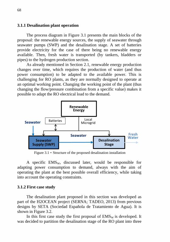
Figure 3.1 – Structure of the proposed desalination installation ..................68
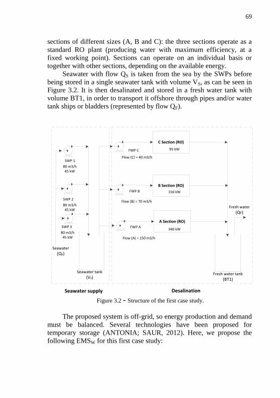
Figure 3.2 – Structure of the first case study ................................................69
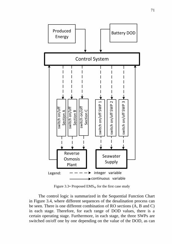
Figure 3.3 – Proposed EMSW for the first case study ..................................71
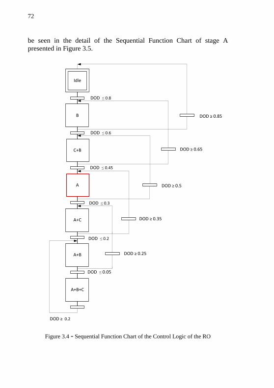
Figure 3.4 – Sequential Function Chart of the Control Logic of the RO .....72
Figure 3.5 – Detail of the Sequential Function Chart (Stage A) ..................73
Figure 3.6 – Scheme of the sizing for the first case study ............................75
Figure 3.7 – Effect of battery capacity (CP) on system performance (VS
5500 m3). ......................................................................................................77
Page 20
Figure 3.8 – Effect of seawater tank volume (VS) on system
performance (Cp 2400 Ah). ......................................................................... 77
Figure 3.9 – Power produced by renewable energies (Pw) .......................... 78
Figure 3.10 – Fresh water produced (QF) in each RO section ..................... 79
Figure 3.11 – Total fresh water produced (QF) ............................................ 79
Figure 3.12 – Total power consumed (PT) ................................................... 79
Figure 3.13 – Stored seawater ...................................................................... 79
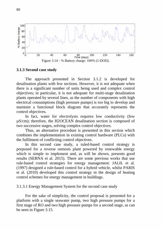
Figure 3.14 – % Battery charge 100%(1-DOD). .......................................... 80
Figure 3.15 – Structure of the second case study ......................................... 81
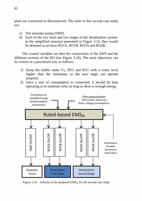
Figure 3.16 – Scheme of the proposed EMSW for the second case study .... 82
Figure 3.17 – Power available (PW) and consumed (PT) by the
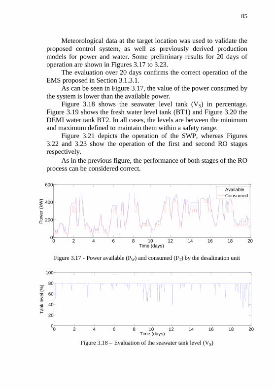
desalination unit ........................................................................................... 85
Figure 3.18 –Evaluation of the seawater tank level (VS) ............................. 85
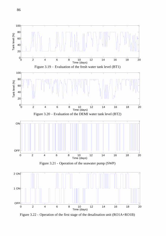
Figure 3.19 – Evaluation of the fresh water tank level (BT1) ...................... 86
Figure 3.20 – Evaluation of the DEMI water tank level (BT2) ................... 86
Figure 3.21 – Operation of the seawater pump (SWP) ................................ 86
Figure 3.22 – Operation of the first stage of the desalination unit
(RO1A+RO1B). ........................................................................................... 86
Figure 3.23 – Operation of the second stage of the desalination unit
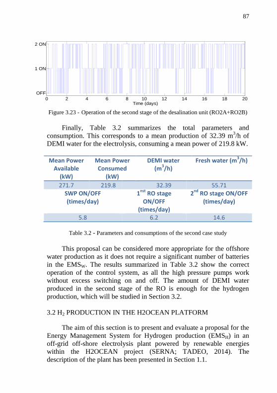
(RO2A+RO2B) ............................................................................................ 87
Figure 3.24 – Process diagram of the hydrogen plant .................................. 88
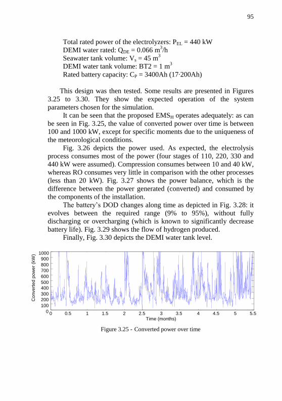
Figure 3.25 – Converted power along time .................................................. 95
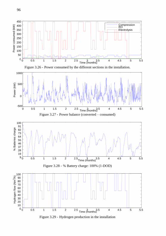
Figure 3.26 – Power consumed by the different sections in the
installation .................................................................................................... 96
Figure 3.27 – Power balance (converted – consumed) ................................ 96
Figure 3.28 – % Batteries charge: 100% (1 – DOD) ................................... 96
Figure 3.29 – Hydrogen production in the installation ................................ 96
Figure 3.30 – DEMI water tank level........................................................... 97
Figure 4.1 – Block structure of the renewable hydrogen plant .................... 103
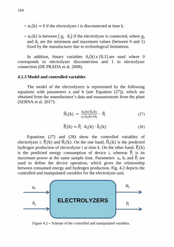
Figure 4.2 – Scheme of the controlled and manipulated variables .............. 104
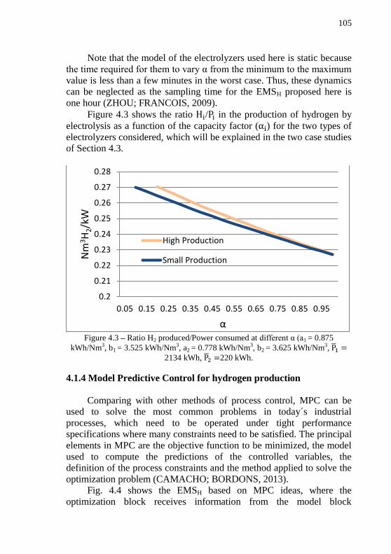
Figure 4.3 – Ratio H2 produced/Power consumed at different α ................. 105
Figure 4.4 – Proposed EMSH based on MPC ideas ...................................... 106
Figure 4.5 – Structure of the EMSH control algorithm................................. 119
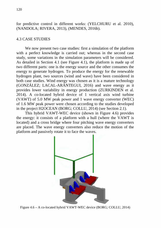
Figure 4.6 – A co-located hybrid VAWT-WEC device ............................... 120
Figure 4.7 – Meteorological predictions of wave period ............................. 121
Figure 4.8 – Meteorological predictions of wave height ............................. 121
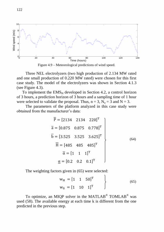
Figure 4.9 – Meteorological predictions of wind speed ............................... 122
Figure 4.10 – Power available and consumed for the first case study ......... 123
Figure 4.11 – Operation of electrolyzer i = 1 for the first case study. ......... 123
Figure 4.12 – Operation of electrolyzer i = 2 for the first case study .......... 124
Figure 4.13 – Operation of electrolyzer i = 3 for the first case study .......... 124
Page 21
Figure 4.14 – Hydrogen production for the first case study .........................125
Figure 4.15 – Power available and consumed for the second case study .....127
Figure 4.16 – Operation of electrolyzer i = 1 for the second case study ......127
Figure 4.17 – Operation of electrolyzer i = 2 for the second case study ......127
Figure 4.18 – Operation of electrolyzer i = 3 for the second case study ......128
Figure 4.19 – Operation of electrolyzer i = 4 for the second case study ......128
Figure 4.20 – Operation of electrolyzer i = 5 for the second case study ......128
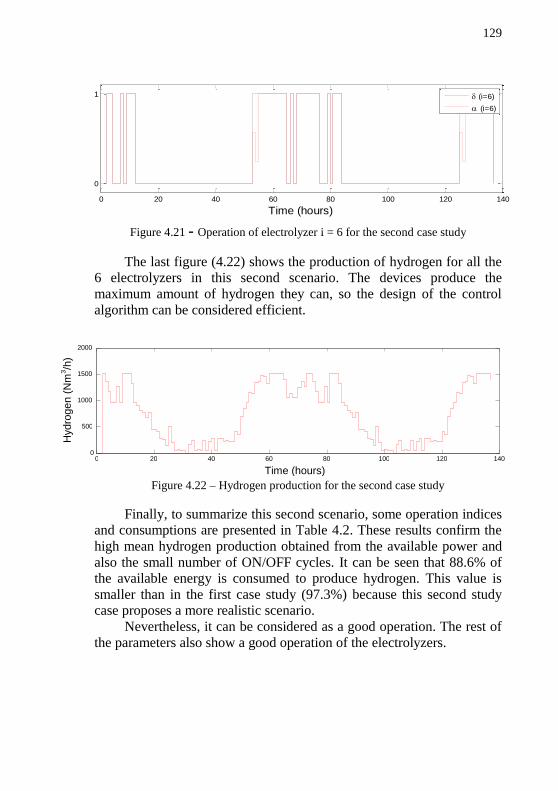
Figure 4.21 – Operation of electrolyzer i = 6 for the second case study ......129
Figure 4.22 – Hydrogen production for the second case study ....................129
Figure 5.1 – Coupling of the Long Term System with the Short Term
System for the hydrogen-based microgrid ...................................................135
Figure 5.2 – Components of the hydrogen-based microgrid ........................138
Figure 5.3 – Activation time (φ) between the on/off state (δ) and the
logical order signal to start-up (Λ) ................................................................144
Figure 5.4 – Block diagram coupling the LTS and the STS.........................146
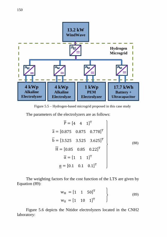
Figure 5.5 – Hydrogen-based microgrid proposed in this case study ..........150
Figure 5.6 – Nitidor electrolyzer in the CNH2 .............................................151
Figure 5.7 – Battery and ultracapacitor in the CNH2 ...................................151
Figure 5.8 – Available renewable power profile ..........................................152
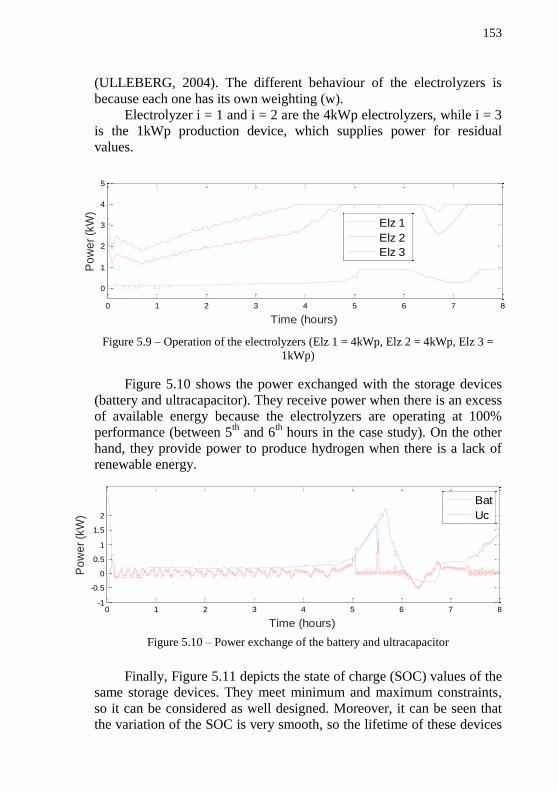
Figure 5.9 – Operation of the electrolyzers (Elz 1 = 4kWp, Elz 2 =
4kWp, Elz 3 = 1kWp) ..................................................................................153
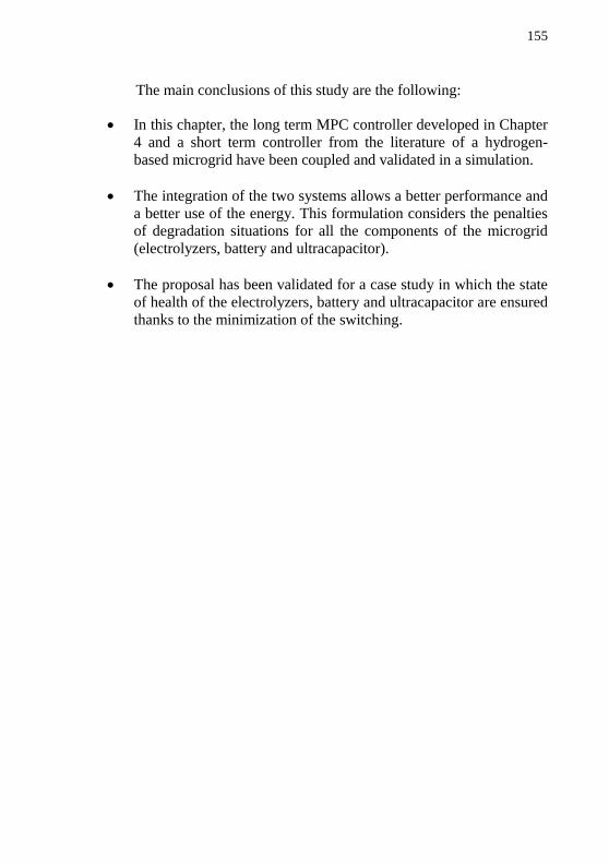
Figure 5.10 – Power exchange of the battery and ultracapacitor .................153
Figure 5.11 – Battery and ultracapacitor SOC .............................................154
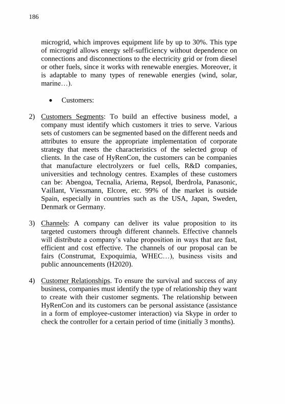
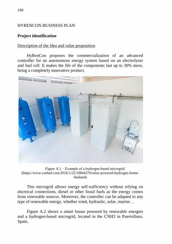
Figure A.1 – Example of a hydrogen-based microgrid ................................190
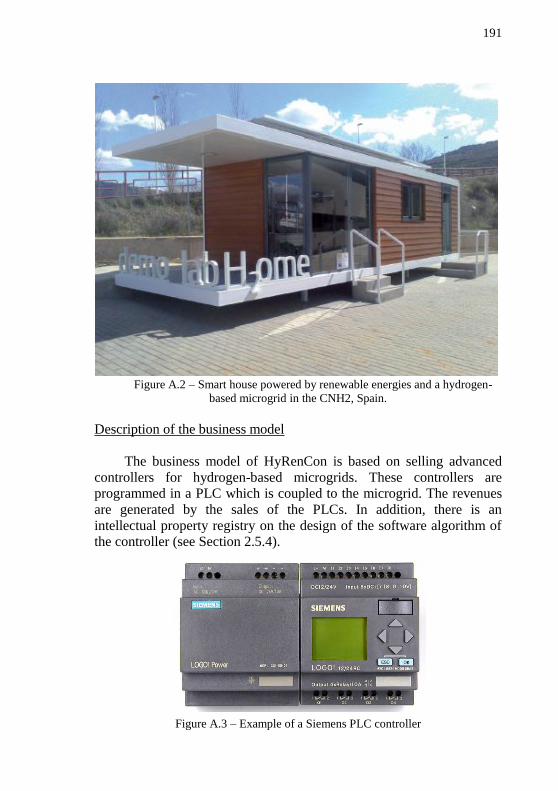
Figure A.2 – Smart house powered by renewable energies and a
hydrogen-based microgrid in the CNH2, Spain ...........................................191
Figure A.3 – Example of a Siemens PLC controller ....................................191
Figure A.4 – Possible customers of HyRenCon ...........................................192
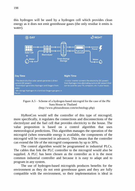
Figure A.5 – Scheme of a hydrogen-based microgrid for the case of the
Phi Suea House in Thailand .........................................................................198
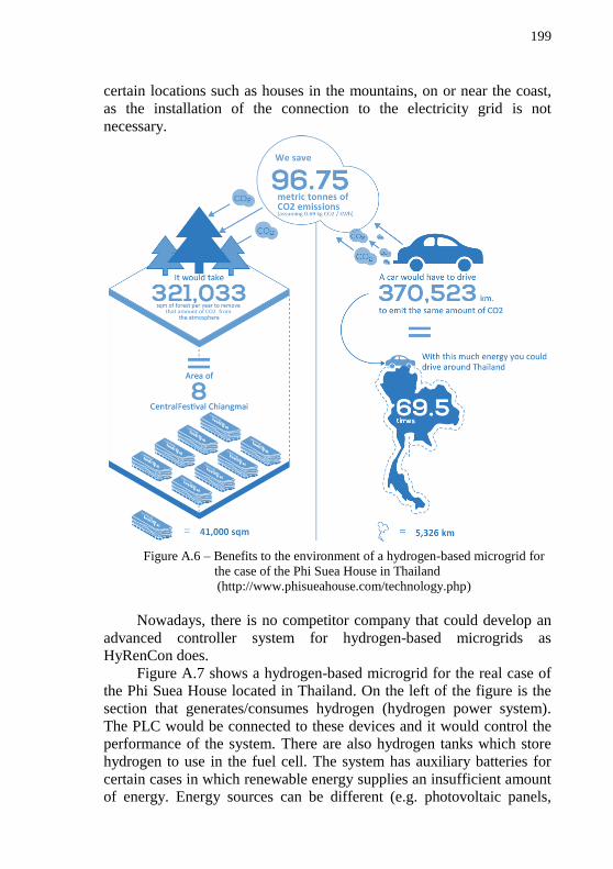
Figure A.6 – Benefits in the environment of a hydrogen-based microgrid
for the case of the Phi Suea House in Thailand ..........................................199
Figure A.7 – Scheme of the components of the hydrogen-based
microgrid ......................................................................................................200
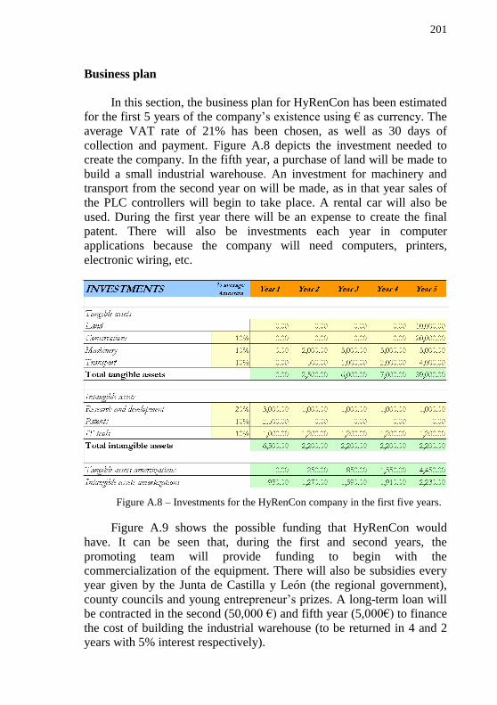
Figure A.8 – Investment for the HyRenCon company for the first five
years .............................................................................................................201
Figure A.9 – Financing for the HyRenCon company for the first five
years .............................................................................................................202
Figure A.10 – Sales for the HyRenCon company for the first five years .....202
Page 22
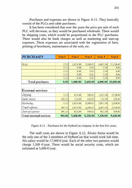
Figure A.11 – Purchases for the HyRenCon company for the first five
years ............................................................................................................. 203
Figure A.12 – Staff costs for the HyRenCon company for the first five
years ............................................................................................................. 204
Figure A.13 – Gains and losses over the first five years .............................. 204
Figure A.14 – Gain and losses for the HyRenCon company for the first
five years ...................................................................................................... 205
Page 23
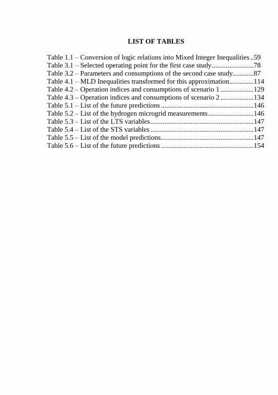
LIST OF TABLES
Table 1.1 – Conversion of logic relations into Mixed Integer Inequalities ..59
Table 3.1 – Selected operating point for the first case study ........................78
Table 3.2 – Parameters and consumptions of the second case study............87
Table 4.1 – MLD Inequalities transformed for this approximation..............114
Table 4.2 – Operation indices and consumptions of scenario 1 ...................129
Table 4.3 – Operation indices and consumptions of scenario 2 ...................134
Table 5.1 – List of the future predictions .....................................................146
Table 5.2 – List of the hydrogen microgrid measurements ..........................146
Table 5.3 – List of the LTS variables ...........................................................147
Table 5.4 – List of the STS variables ...........................................................147
Table 5.5 – List of the model predictions .....................................................147
Table 5.6 – List of the future predictions .....................................................154
Page 24
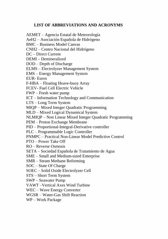
LIST OF ABBREVIATIONS AND ACRONYMS
AEMET – Agencia Estatal de Meteorología
AeH2 – Asociación Española de Hidrógeno
BMC – Business Model Canvas
CNH2 – Centro Nacional del Hidrógeno
DC – Direct Current
DEMI – Demineralized
DOD – Depth of Discharge
ELMS – Electrolyzer Management System
EMS – Energy Management System
EUR- Euros
F-HBA – Floating Heave-buoy Array
FCEV- Fuel Cell Electric Vehicle
FWP – Fresh water pump
ICT – Information Technology and Communication
LTS – Long Term System
MIQP – Mixed Integer Quadratic Programming
MLD – Mixed Logical Dynamical System
NLMIQP – Non Linear Mixed Integer Quadratic Programming
PEM – Proton Exchange Membrane
PID – Proportional-Integral-Derivative controller
PLC – Programmable Logic Controller
PNMPC – Practical Non-Linear Model Predictive Control
PTO – Power Take Off
RO – Reverse Osmosis
SETA – Sociedad Española de Tratamiento de Agua
SME – Small and Medium-sized Enterprise
SMR – Steam Methane Reforming
SOC – State Of Charge
SOEC – Solid Oxide Electrolyzer Cell
STS – Short Term System
SWP – Seawater Pump
VAWT –Vertical Axes Wind Turbine
WEC – Wave Energy Converter
WGSR – Water-Gas Shift Reaction
WP – Work Package
Page 25
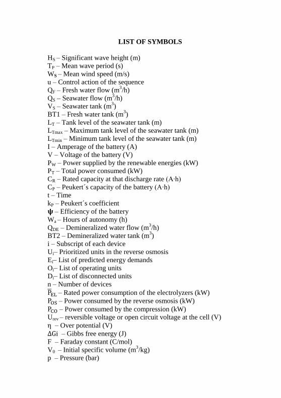
LIST OF SYMBOLS
HS – Significant wave height (m)
TP – Mean wave period (s)
WS – Mean wind speed (m/s)
u – Control action of the sequence
QF – Fresh water flow (m3/h)
QS – Seawater flow (m3/h)
VS – Seawater tank (m3)
BT1 – Fresh water tank (m3)
LT – Tank level of the seawater tank (m)
LTmax – Maximum tank level of the seawater tank (m)
LTmin – Minimum tank level of the seawater tank (m)
I – Amperage of the battery (A)
V – Voltage of the battery (V)
PW – Power supplied by the renewable energies (kW)
PT – Total power consumed (kW)
CR – Rated capacity at that discharge rate (A∙h)
CP – Peukert´s capacity of the battery (A∙h)
t – Time
kP – Peukert´s coefficient
𝛙 – Efficiency of the battery
Wa – Hours of autonomy (h)
QDE – Demineralized water flow (m3/h)
BT2 – Demineralized water tank (m3)
i – Subscript of each device
Ui– Prioritized units in the reverse osmosis
Ei– List of predicted energy demands
Oi– List of operating units
Di– List of disconnected units
n – Number of devices
PEL – Rated power consumption of the electrolyzers (kW)
POS – Power consumed by the reverse osmosis (kW)
PCO – Power consumed by the compression (kW)
Urev – reversible voltage or open circuit voltage at the cell (V)
η – Over potential (V)
ΔGi – Gibbs free energy (J)
F – Faraday constant (C/mol)
V0 – Initial specific volume (m3/kg)
p – Pressure (bar)
Page 26
R – Gas constant (J/mol)
γ – Ratio of specific heats
T – Temperature (K)
Epro – Activation energy for proton transport in the membrane (J/mol)
Eexc – Activation energy for the electrode reaction (J/mol)
π – Conductivity of the membrane (S/m)
RE – Resistive loss (Ω)
tm – Thickness of the membrane (m)
ac – Activity coefficient
i0 – Exchange current density (A/m2)
λ – Charge transfer coefficients
N – Prediction horizon
Nu – Control horizon
i – Subscript of each device
δi (k) – Binary variable: ON/OFF electrolysis unit i at instant k
δi (k) – Prediction of the binary variable of unit i at instant k
αi (k) – Capacity factor of electrolysis unit i at instant k
αi (k) – Prediction of the capacity factor of unit i at instant k
zi (k) – Auxiliary variable of electrolysis unit i at instant k
Δzi (k) – Increase of the auxiliary variable of unit i at instant k
Δzi (k) – Prediction of the increase of the auxiliary variable
Hi (k) – Hydrogen production of electrolysis unit i at instant k (Nm3/h)
Hi (k) – Prediction of the hydrogen production of unit i at instant k
Hi – Maximum H2 production (Nm3/h) of electrolysis unit i
ai – Slope of power model of electrolysis unit i (kWh/ Nm3)
bi – Offset of power model of electrolysis unit i (kWh/ Nm3)
αi αi – Minimum and maximum capacity factor of unit i
Pi (k) – Power consumption of electrolysis unit i at instant k (kW)
Pavailable (k) – Prediction of power available at instant k (kW)
wH – Weighting factor of the error
wδ – Weighting factor of the control variable
J – Quadratic cost function (Nm3/h)
T– Triangular matrix
gi (k) – Optimization model of electrolysis unit i at instant k
Q – Quadratic part of the cost function
L – Linear part of the cost function
A, B – Constraints matrices
f – Free response vector
G – System’s dynamic matrix
∆u – Vector of control increments
Page 27
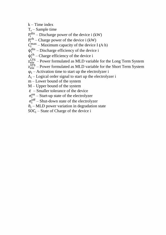
k – Time index
Ts – Sample time
Pidis – Discharge power of the device i (kW)
Pich – Charge power of the device i (kW)
Cimax – Maximum capacity of the device I (A∙h)
ψidis – Discharge efficiency of the device i
ψich – Charge efficiency of the device i
zeleLTS – Power formulated as MLD variable for the Long Term System
zeleSTS – Power formulated as MLD variable for the Short Term System
φi – Activation time to start up the electrolyzer i
Λi – Logical order signal to start up the electrolyzer i
m – Lower bound of the system
M – Upper bound of the system
ε – Smaller tolerance of the device
σion – Start-up state of the electrolyzer
σioff – Shut-down state of the electrolyzer
ϑi – MLD power variation in degradation state
SOCi – State of Charge of the device i
Page 29
SUMMARY
1 INTRODUCTION .............................................................. 29 1.1 MOTIVATION ............................................................................ 29
1.2 OBJECTIVES .............................................................................. 31
2 STATE OF THE ART ....................................................... 35 2.1 RENEWABLE ENERGIES ......................................................... 35
2.1.1 Wave Energy .............................................................................. 36 2.1.2 Wind Energy .............................................................................. 41 2.2 REVERSE OSMOSIS ................................................................. 44
2.3 HYDROGEN ............................................................................... 46 2.3.1 Hydrogen production................................................................. 47 2.3.1.1 Black Hydrogen ........................................................................... 48 2.3.1.2 Green Hydrogen ........................................................................... 51 2.3.1.3 Blue Hydrogen ............................................................................. 51 2.4 MODEL PREDICTIVE CONTROL ........................................... 56
2.4.1 MPC strategy.............................................................................. 56
2.4.2 Receding horizon ........................................................................ 58
2.4.3 Constraints ................................................................................. 59
2.5 CONTRIBUTIONS ..................................................................... 60
2.5.1 Journal papers............................................................................ 60 2.5.2 Conference papers ..................................................................... 60
2.5.3 Other contributions ................................................................... 61 2.5.4 Patent and intellectual property registration .......................... 62 2.6 ORGANIZATION OF THE THESIS .......................................... 63
2.7 SUMMARY AND CONCLUSIONS .......................................... 64
3 CONTROL OF THE H2OCEAN PLATFORM .............. 67 3.1 FRESH H2O PRODUCTION IN THE H2OCEAN PLATFORM 67
3.1.1 Desalination plant operation ...................................................... 68
3.1.2 First case study ............................................................................ 68
3.1.2.1 Energy Management System based on heuristic control ............... 70
3.1.2.2 Sizing of the first case study ......................................................... 74
3.1.2.3 Results and discussion .................................................................. 75
3.1.3 Second case study ........................................................................ 80
3.1.3.1 Energy Management System ........................................................ 80
3.1.3.2 Results and discussion .................................................................. 84
3.2 H2 PRODUCTION IN THE H2OCEAN PLATFORM ................ 87
3.2.1 Hydrogen plant operation for hydrogen production ............... 88
3.2.2 Energy Management System...................................................... 89
3.2.3 Sizing and modelling ................................................................... 89
3.2.3.1 Electrolyzers ................................................................................. 90
3.2.3.2 Hydrogen compression ................................................................. 93
3.2.3.3 Electricity storage ......................................................................... 94
Page 30
3.2.4 Results and discussion ................................................................ 94
3.3 SUMMARY AND CONCLUSIONS .......................................... 97
4 ENERGY MANAGEMENT SYSTEM FOR HYDROGEN
PRODUCTION BASED ON MPC ................................................ 101 4.1 MATERIALS AND METHOD .................................................... 102
4.1.1 Process description ..................................................................... 102
4.1.2 Manipulated variables ................................................................ 103
4.1.3 Model and controlled variables ................................................. 104
4.1.4 Model Predictive Control for hydrogen production ................ 105
4.2 PROPOSED ENERGY MANAGEMENT SYSTEM .................. 107
4.2.1 Control objectives ....................................................................... 107
4.2.2 Cost function and optimization problem .................................. 107
4.2.3 Approximation to an MIQP ....................................................... 109
4.2.4 Constraints .................................................................................. 113
4.2.5 Optimization ............................................................................... 114
4.2.6 MPC strategy .............................................................................. 118
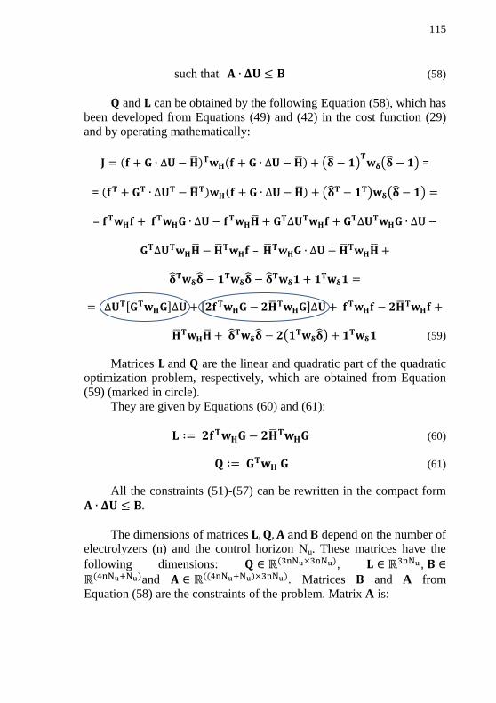
4.3 CASE STUDIES........................................................................... 120
4.3.1 First case study............................................................................ 121
4.3.2 Second case study ........................................................................ 125
4.4 SUMMARY AND CONCLUSIONS ........................................... 130
5 COUPLING OF A LOW LEVEL SYSTEM WITH A HIGH
LEVEL SYSTEM IN A H2 MICROGRID ................................... 135 5.1 HYDROGEN-BASED MICROGRIDS ........................................ 136
5.1.1 Components of the hydrogen-based microgrid ........................ 137
5.1.2 Electrolyzers ................................................................................ 138
5.1.3 Batteries and ultracapacitor ...................................................... 139
5.2 LONG TERM SYSTEM .............................................................. 140
5.2.1 Long term MPC design .............................................................. 141
5.1.2 Control objectives of the LTS .................................................... 141
5.3 SHORT TERM SYSTEM ............................................................ 143
5.3.1 Short term MPC design .............................................................. 145
5.3.2 Control objectives of the STS .................................................... 147
5.3.2.1 Ultracapacitor cost function .......................................................... 148
5.3.2.2 Battery cost function ..................................................................... 148
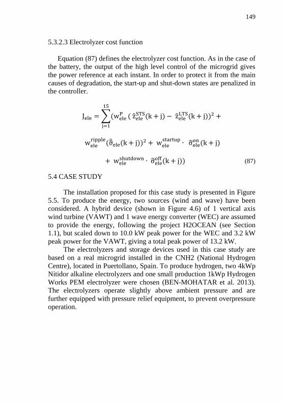
5.3.2.3 Electrolyzer cost function ............................................................. 149
5.4 CASE STUDY .............................................................................. 149
5.4.1 Controller implementation......................................................... 152
5.4.2 Results and discussion ................................................................ 152
5.5 SUMMARY AND CONCLUSIONS ........................................... 154
6 CONCLUSIONS ................................................................. 159 6.1 FINAL CONCLUSIONS .............................................................. 159
Page 31
6.2 FUTURE WORK .......................................................................... 161
ACKNOWLEDGEMENTS .............................................. 163
REFERENCES................................................................... 164
ANNEX ............................................................................... 183
Page 33
27
CHAPTER 1
INTRODUCTION
Page 35
29
1 INTRODUCTION
1.1 MOTIVATION
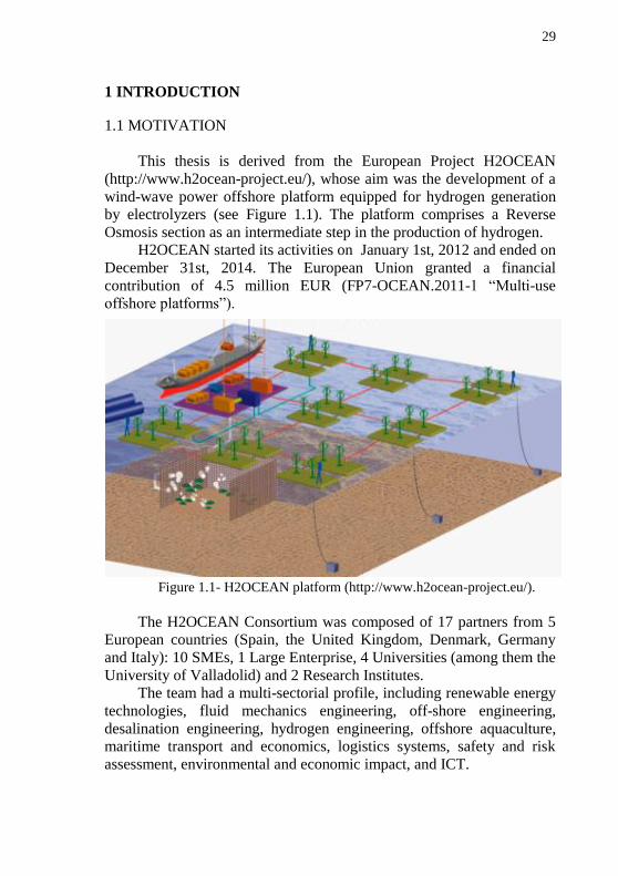
This thesis is derived from the European Project H2OCEAN
(http://www.h2ocean-project.eu/), whose aim was the development of a
wind-wave power offshore platform equipped for hydrogen generation
by electrolyzers (see Figure 1.1). The platform comprises a Reverse
Osmosis section as an intermediate step in the production of hydrogen.
H2OCEAN started its activities on January 1st, 2012 and ended on
December 31st, 2014. The European Union granted a financial
contribution of 4.5 million EUR (FP7-OCEAN.2011-1 “Multi-use
offshore platforms”).
Figure 1.1- H2OCEAN platform (http://www.h2ocean-project.eu/).
The H2OCEAN Consortium was composed of 17 partners from 5
European countries (Spain, the United Kingdom, Denmark, Germany
and Italy): 10 SMEs, 1 Large Enterprise, 4 Universities (among them the
University of Valladolid) and 2 Research Institutes.
The team had a multi-sectorial profile, including renewable energy
technologies, fluid mechanics engineering, off-shore engineering,
desalination engineering, hydrogen engineering, offshore aquaculture,
maritime transport and economics, logistics systems, safety and risk
assessment, environmental and economic impact, and ICT.
Page 36
30
Figure 1.2- Participants in H2OCEAN Project.
The University of Valladolid was the leader of Work Package 5.
The goals of this WP5 were the development and dimensioning of a
hydrogen installation for offshore platforms. The work done included:
1. Evaluation of existing electrolyzing technologies for marine
environments (AGERSTED, 2014).
2. Design of offshore desalination units for hydrogen generation
(TORRIJOS, 2012).
3. Development of an Energy Management System (EMS) for the
offshore hydrogen installation to minimize energy consumption
and balance production and consumption of energy (SERNA et
al. 2017).
The unique feature of the H2OCEAN concept, besides the
integration of different activities into a shared multi-use installation, was
the novel approach for the transmission of offshore-generated renewable
electrical energy through hydrogen. This concept allows effective
transport and storage of the energy, decoupling energy production and
consumption, thus avoiding the grid imbalance problem inherent to
current offshore renewable energy systems. Additionally, it circumvents
the need for a cable transmission system which takes up a significant
Page 37
31
investment share for offshore energy generation infrastructures,
increasing the price of energy (BAUER; LYSGAARD, 2015).
Offshore power links are known to be significantly expensive
(RUDDY et al. 2016), so the system is here assumed to be fully isolated
from the grid. Thus, the EMS balances power consumption with
production by connecting or disconnecting sections of the
electrolyzation plant (following a Smart Grid approach for the microgrid
in the plant), and using temporary storage of electricity for short-term
balances and increased autonomy (which is a relevant issue in offshore
installations). The importance of designing a control system to balance
the energy provided from renewable sources and the energy consumed
by the components of the installation (reverse osmosis, hydrogen
production, storage, etc.) was considered a key factor for its correct
operation. Therefore, the operation of the devices using an advanced
control strategy based on model predictive control ideas is very relevant
for these systems (MELO; CHANG CHIEN, 2014), so it is the focus of
the current thesis.
1.2 OBJECTIVES OF THE THESIS
The main objective of this thesis named, “Control system of
offshore hydrogen production by renewable energies”, is to develop an
Energy Management System (EMS) based on Model Predictive Control
(MPC) ideas that balances energy consumption with the renewable
energy supplied in stand-alone installations, in particular for offshore
installations.
For this, the modelling of the renewable energy sources (wave and
wind energy), plus the design of a control proposal for water generation
by reverse osmosis, and hydrogen production by electrolysis focusing on
the H2OCEAN platform is first carried out (Chapter 3).
Then, an advanced control system of the electrolysis section,
numerically optimizing the state-of-health of the devices, is developed
in Chapter 4.
Chapter 5 evaluates the coupling of low and high level controllers
of the hydrogen-based microgrids made up of electrolyzers, batteries
and ultracapacitor.
Finally, an economic study and a business plan for the
implantation of the controlled hydrogen-based microgrid in the market
are carried out in Annex A.
Page 39
33
CHAPTER 2
STATE OF THE ART
Page 41
35
2 STATE OF THE ART
2.1 RENEWABLE ENERGIES
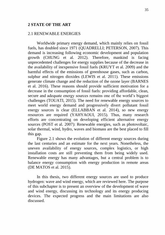
Worldwide primary energy demand, which mainly relies on fossil
fuels, has doubled since 1971 (QUADRELLI; PETERSON, 2007). This
demand is increasing following economic development and population
growth (CHUNG et al. 2012). Therefore, mankind is facing
unprecedented challenges for energy supplies because of the decrease in
the availability of inexpensive fossil fuels (KRUYT et al. 2009) and the
harmful effects of the emissions of greenhouse gases, such as carbon,
sulphur and nitrogen dioxides (LEWIS et al. 2011). These emissions
generate climate change and the reduction of the ozone layer (BARNES
et al. 2016). These reasons should provide sufficient motivation for a
decrease in the consumption of fossil fuels: providing affordable, clean,
secure and adequate energy sources remains one of the world’s biggest
challenges (TOUATI, 2015). The need for renewable energy sources to
meet world energy demand and progressively divert pollutant fossil
energy sources is clear (ELLABBAN et al. 2014), so new energy
resources are required (YAHYAOUI, 2015). Thus, many research
efforts are concentrating on developing efficient alternative energy
sources (POST et al. 2007): Renewable energies, such as photovoltaic,
solar thermal, wind, hydro, waves and biomass are the best placed to fill
this gap.
Figure 2.1 shows the evolution of different energy sources during
the last centuries and an estimate for the next years. Nonetheless, the
uneven availability of energy sources, complex logistics, or high
installation costs are still preventing them from being widely used.
Renewable energy has many advantages, but a central problem is to
balance energy consumption with energy production in remote areas
(DE MATOS et al. 2015).
In this thesis, two different energy sources are used to produce
hydrogen: wave and wind energy, which are reviewed here. The purpose
of this subchapter is to present an overview of the development of wave
and wind energy, discussing its technology and its energy producing
devices. The expected progress and the main limitations are also
discussed.
Page 42
36
Figure 2.1- Share of US primary energy demand, 1780-2100. (ROSER, 2016)
2.1.1 Wave energy
Wave energy can be extracted easily from the oceans to generate
renewable energy to fulfil human requirements (ZURKINDEN et al.
2014). In comparison with other energy sources, it is less developed
than wind, photovoltaic and fossil fuel technologies (CLÉMENT et al.
2002). Different studies have evaluated this technology in different
locations around the world, for example in the Atlantic Ocean
(IGLESIAS et al. 2009), the Pacific Ocean (LENEE-BLUHM et al.
2011) or the Mediterranean Sea (LIBERTI et al. 2013). Figure 2.2
depicts the flux of wave energy in the oceans and seas worldwide. These
studies indicate the potential hydrodynamic power in each location in
order to get an approximation of the energy that can be absorbed by a
device (converter) which transforms mechanical energy into electricity.
Wave energy is an indirect form of energy (ANTONIO, 2010), as it is in
fact wind that generates waves. When arriving at wave energy
converters, these waves give some of their energy, which is converted
into electricity. Similarly to wind energy, the main drawback of wave
energy is its variability on several time-scales (GARRET; MUNK,
1975): from wave to wave, with the state of the sea, and from month to month.
Page 43
37
Figure 2.2- World map of wave energy flux in kW per meter wave front.
(http://www.newslettereuropean.eu/new-way-wave-tidal-energy/).
The energy produced by waves depends on the wave period (TP)
and height (HS). Figures 2.3 and 2.4 show these parameters in a certain
location in the North Atlantic Ocean over 1 month in winter. It is these
parameters that are used in this thesis (Chapter 3). As can be seen, they
vary because of meteorological conditions:
Figure 2.3- Mean wave period in January in North Atlantic Ocean
(ROC, 2014)
Figure 2.4- Significant wave height in January in North Atlantic Ocean (ROC,
2014)
0 5 10 15 20 25 300
2
4
6
8
Time (days)
Wa
ve
heig
ht
(m)
0 5 10 15 20 25 304
6
8
10
12
14
Time (days)
Wa
ve
perio
d (
s)
Page 44
38
Wave energy converters
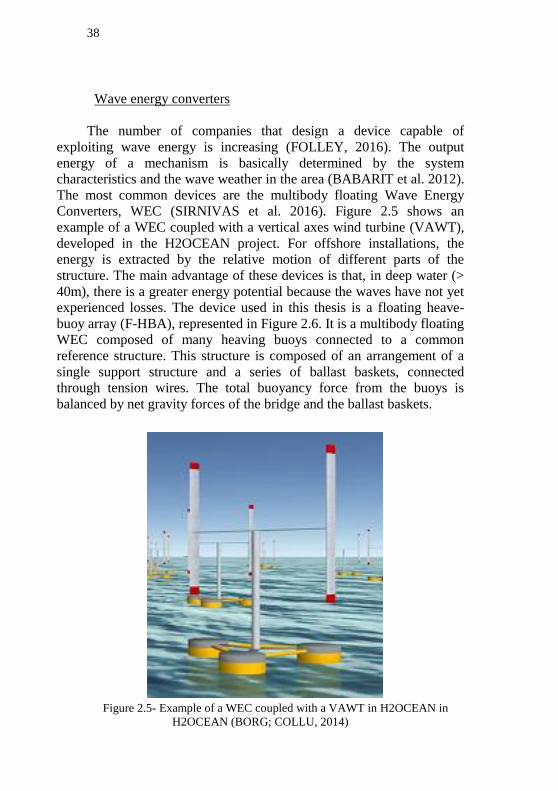
The number of companies that design a device capable of
exploiting wave energy is increasing (FOLLEY, 2016). The output
energy of a mechanism is basically determined by the system
characteristics and the wave weather in the area (BABARIT et al. 2012).
The most common devices are the multibody floating Wave Energy
Converters, WEC (SIRNIVAS et al. 2016). Figure 2.5 shows an
example of a WEC coupled with a vertical axes wind turbine (VAWT),
developed in the H2OCEAN project. For offshore installations, the
energy is extracted by the relative motion of different parts of the
structure. The main advantage of these devices is that, in deep water (>
40m), there is a greater energy potential because the waves have not yet
experienced losses. The device used in this thesis is a floating heave-
buoy array (F-HBA), represented in Figure 2.6. It is a multibody floating
WEC composed of many heaving buoys connected to a common
reference structure. This structure is composed of an arrangement of a
single support structure and a series of ballast baskets, connected
through tension wires. The total buoyancy force from the buoys is
balanced by net gravity forces of the bridge and the ballast baskets.
Figure 2.5- Example of a WEC coupled with a VAWT in H2OCEAN in
H2OCEAN (BORG; COLLU, 2014)
Page 45
39
Ballast
Tension wires
Support structure
Heaving buoys
Figure 2.6- Scheme of the WEC proposed in H2OCEAN
Figure 2.7 depicts the average power output that can be absorbed
by the specific wave energy converter (WEC) shown in Figure 2.5,
taking into account meteorological parameters described previously of
mean wave period and significant wave height.
Figure 2.7- Average power output provided by a 2.2 MW WEC using data of
Figs.2.3-2.4.
The buoys are connected to the submerged structure via a
hydraulic Power Take-Off (PTO) system, which converts the
mechanical energy of the device into electricity. In the case of wave
activated body WECs, they can be based on hydraulic components
(hydraulic rams and motors) combined with an electrical generator
(HENDERSON, 2006), or they can be fully electrical (ERIKSSON,
2007 and RUELLAN et al. 2010), which was assumed in this thesis due
to the special conditions of offshore platforms.
One of the key points in the structural design and energy extraction
capacity of the device is the response to different periods and wave
0 5 10 15 20 25 300
0.5
1
1.5
2
2.5
Time (days)
Wa
ve
Pow
er
(MW
)
Page 46
40
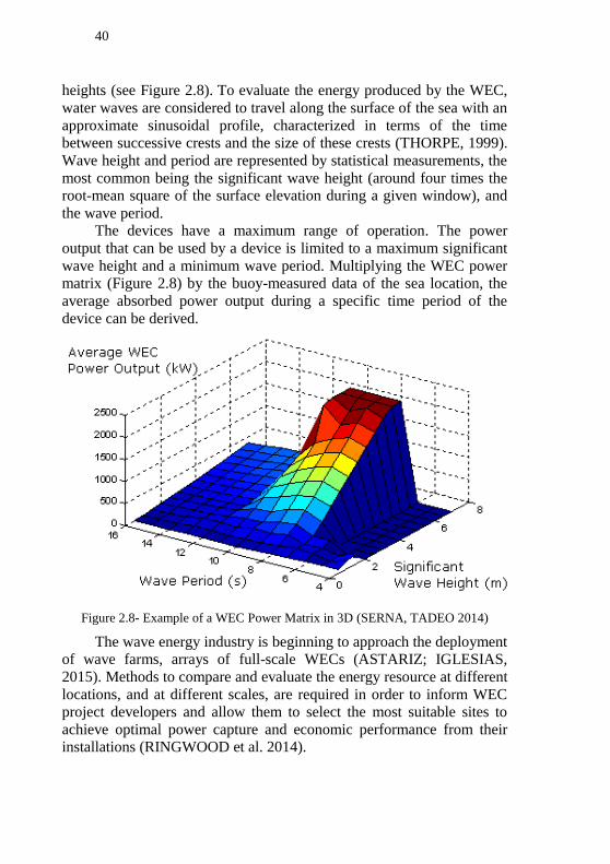
heights (see Figure 2.8). To evaluate the energy produced by the WEC,
water waves are considered to travel along the surface of the sea with an
approximate sinusoidal profile, characterized in terms of the time
between successive crests and the size of these crests (THORPE, 1999).
Wave height and period are represented by statistical measurements, the
most common being the significant wave height (around four times the
root-mean square of the surface elevation during a given window), and
the wave period.
The devices have a maximum range of operation. The power
output that can be used by a device is limited to a maximum significant
wave height and a minimum wave period. Multiplying the WEC power
matrix (Figure 2.8) by the buoy-measured data of the sea location, the
average absorbed power output during a specific time period of the
device can be derived.
Figure 2.8- Example of a WEC Power Matrix in 3D (SERNA, TADEO 2014)
The wave energy industry is beginning to approach the deployment
of wave farms, arrays of full-scale WECs (ASTARIZ; IGLESIAS,
2015). Methods to compare and evaluate the energy resource at different
locations, and at different scales, are required in order to inform WEC
project developers and allow them to select the most suitable sites to
achieve optimal power capture and economic performance from their
installations (RINGWOOD et al. 2014).
Page 47
41
2.1.2 Wind energy
Wind energy is a renewable energy source which is obtained from
air masses in movement (BURTON et al. 2001). Electric power is
generated by a turbine that converts a portion of the kinetic energy from
the wind into mechanical energy (BIANCHI et al. 2007). This
technology has matured to a level of development where it is generally
accepted (GONZÁLEZ; LACAL-ARÁNTEGUI, 2016). Wind power is
already playing an important role in electricity generation, especially in
countries such as Germany, Denmark, Korea or Spain (PÉREZ-
COLLADO et al. 2015), (HOU et al. 2017), (KIM; KIM, 2017). World
wind energy resources are substantial, and in many areas, such as the US
and Northern Europe, could in theory supply all of the electricity
demand (JACOBSON; DELUCCHI, 2011). However, the intermittent
character of the wind resources and the necessity of long distances for
energy transmission are considered the main drawbacks of wind energy.
Nowadays offshore farms are a promising technology (ESTEBAN
et al. 2011) and there is considerable hope that offshore wind farms may
be the solution (NG; RAN, 2016). Vast offshore areas are characterized
by higher and more reliable wind resources in comparison with
continental areas. However, offshore wind energy production is in a
quite preliminary phase (BALOG et al. 2016). There have been many
successes with offshore wind farms in Europe since installations began
in 1991 (SUBRAMANI; JACANGELO, 2014).
Vertical Axes Wind Turbine
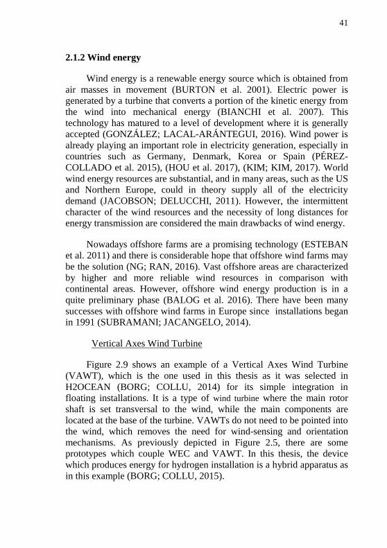
Figure 2.9 shows an example of a Vertical Axes Wind Turbine
(VAWT), which is the one used in this thesis as it was selected in
H2OCEAN (BORG; COLLU, 2014) for its simple integration in
floating installations. It is a type of wind turbine where the main rotor
shaft is set transversal to the wind, while the main components are
located at the base of the turbine. VAWTs do not need to be pointed into
the wind, which removes the need for wind-sensing and orientation
mechanisms. As previously depicted in Figure 2.5, there are some prototypes which couple WEC and VAWT. In this thesis, the device
which produces energy for hydrogen installation is a hybrid apparatus as
in this example (BORG; COLLU, 2015).
Page 48
42
Figure 2.9- Example of a 30-100kW Vertical Axes Wind Turbine in UK
(https://bobbischof.com/about/vertical-axis-wind-turbines-for-micro-generation/).
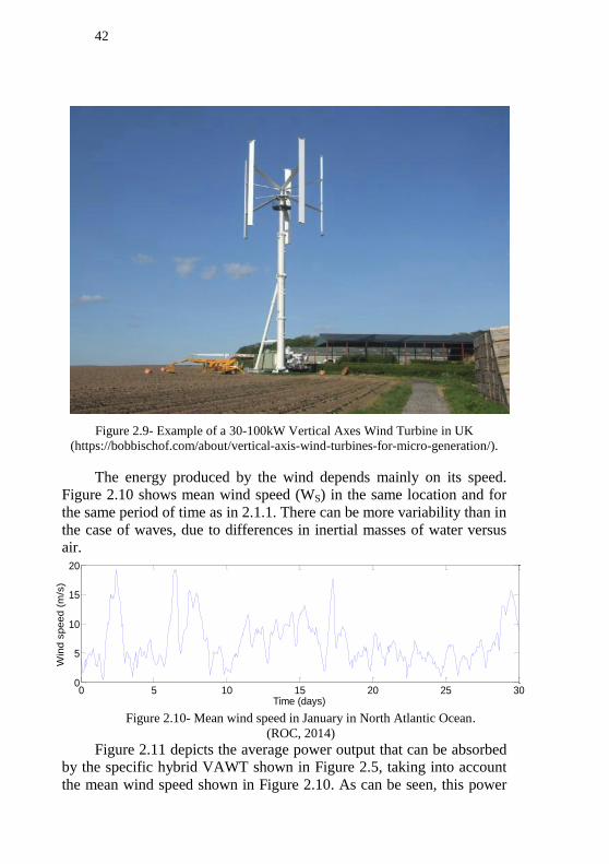
The energy produced by the wind depends mainly on its speed.
Figure 2.10 shows mean wind speed (WS) in the same location and for
the same period of time as in 2.1.1. There can be more variability than in
the case of waves, due to differences in inertial masses of water versus
air.
Figure 2.10- Mean wind speed in January in North Atlantic Ocean.
(ROC, 2014)
Figure 2.11 depicts the average power output that can be absorbed
by the specific hybrid VAWT shown in Figure 2.5, taking into account
the mean wind speed shown in Figure 2.10. As can be seen, this power
0 5 10 15 20 25 300
5
10
15
20
Time (days)
Win
d s
peed (
m/s
)
Page 49
43
is even more variable than wave power and depends strongly on
meteorological conditions.
Figure 2.11- Average power output provided by a 5 MW VAWT using data of
Figs.2.10
Wind turbines have a maximum range of operation. The average
power output that can be used by a device is limited to a certain range of
mean wind speeds. Figure 2.12 shows the relationship between power
output and mean wind speed in this specific VAWT:
Figure 2.12- Power profile of the VAWT developed in the H2Ocean project.
Unlike in the case of wave energy, in which energy depends on
two variables (wave period and height), wind energy only depends on
one variable (wind speed). Moreover, each VAWT has its own power
profile that depends on the wind speed and the VAWT characteristics.
0 5 10 15 20 25 300
2
4
6
Time (days)
Win
d P
ow
er
(MW
)
0 5 10 15 20 25 300
1
2
3
4
5
6
Wind speed (m/s)
Pow
er
pro
duce
d (
MW
)
Page 50
44
2.2 REVERSE OSMOSIS
Reverse Osmosis (RO) is an intermediate step which desalinates
seawater to produce demineralized water, because electrolysis only
operates with low conductivity water (less than a few µS). In the last
few decades, different techniques for fresh water production have been
developed. RO has become the most popular desalination technology
(especially for large-scale seawater desalination plants) (GUDE, 2016).
The required plant capacity, the product cost, the technology maturity
and the coupling of the renewable energy and the desalination systems
(GARCÍA-RODRÍGUEZ, 2003) determine RO as the best option for the
case proposed in this thesis. Figure 2.13 depicts a typical industrial RO
system.
Figure 2.13- Industrial Reverse Osmosis system
(http://www.pureaqua.com/what-is-reverse-osmosis-ro/).
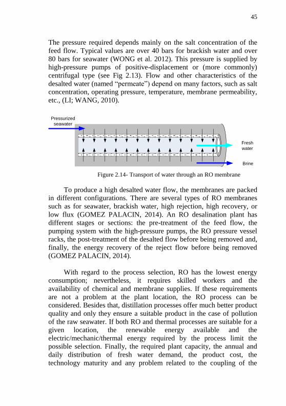
RO is a technique that uses a semipermeable membrane to remove
ions, molecules and large particles from seawater to produce drinkable
water (see Figure 2.14). In this technology, pressure is applied to
overcome the osmotic pressure, a colligative property that is driven by
chemical potential differences of the solvent. The result is that the solute
is retained on the pressurized side of the membrane, so pure water is
allowed to pass to the other side (AMBASHTA; SILLANPÄÄ, 2012).
Page 51
45
The pressure required depends mainly on the salt concentration of the
feed flow. Typical values are over 40 bars for brackish water and over
80 bars for seawater (WONG et al. 2012). This pressure is supplied by
high-pressure pumps of positive-displacement or (more commonly)
centrifugal type (see Fig 2.13). Flow and other characteristics of the
desalted water (named “permeate”) depend on many factors, such as salt
concentration, operating pressure, temperature, membrane permeability,
etc., (LI; WANG, 2010).
Fresh
water
Brine
Pressurized
seawater
Figure 2.14- Transport of water through an RO membrane
To produce a high desalted water flow, the membranes are packed
in different configurations. There are several types of RO membranes
such as for seawater, brackish water, high rejection, high recovery, or
low flux (GOMEZ PALACIN, 2014). An RO desalination plant has
different stages or sections: the pre-treatment of the feed flow, the
pumping system with the high-pressure pumps, the RO pressure vessel
racks, the post-treatment of the desalted flow before being removed and,
finally, the energy recovery of the reject flow before being removed
(GOMEZ PALACIN, 2014).
With regard to the process selection, RO has the lowest energy
consumption; nevertheless, it requires skilled workers and the
availability of chemical and membrane supplies. If these requirements
are not a problem at the plant location, the RO process can be
considered. Besides that, distillation processes offer much better product
quality and only they ensure a suitable product in the case of pollution
of the raw seawater. If both RO and thermal processes are suitable for a
given location, the renewable energy available and the
electric/mechanic/thermal energy required by the process limit the
possible selection. Finally, the required plant capacity, the annual and
daily distribution of fresh water demand, the product cost, the
technology maturity and any problem related to the coupling of the
Page 52
46
renewable energy and the desalination systems determine the selection
(GARCÍA-RODRÍGUEZ, 2003).
Offshore desalination plants powered by renewable energies are
being proposed as an alternative for a coastal desalination facility, for
those locations where the lack of suitable land makes a land-based
desalination plant inadequate (DAVIES, 2005). This is an offshore
plant, which makes the implementation of distillation processes difficult.
Thus, RO was selected as the desalination technique.
2.3 HYDROGEN
Hydrogen has been considered as an energy source since the
nineteenth century (HAMACHER, 2016). Because of global climate
change, carbon emissions into the atmosphere should be gradually
restricted (OPPENHEIMER; ANTTILA-HUGHES, 2016). Therefore,
current energy sources which feed homes, industries and transport
should be gradually replaced by alternative sources (GARCÍA-CLÚA,
2013). Hydrogen is a clean energy carrier independent of energy sources
(SUBRAMANI et al. 2016) and, when it is produced from renewable
energies, offers significant advantages (PANWAR et al. 2011). It is still
not a primary energy source such as oil or coal, although it can be
considered as an excellent energy vector. One advantage of hydrogen in
comparison with other energy sources is that it is everywhere. For
example, in water it is bound with oxygen, which is one of the most
abundant components on Earth, but it also can be linked with carbon in
compounds such as natural gas, coal or biomass.
Nowadays, the most common method to produce hydrogen is the
extraction of natural gas by steam reforming. However, this method
generates greenhouse gases and purity is not sufficient for fuel cells
which require a hydrogen purity of 99.99% (DAVIDS et al. 2016).
Furthermore, it is more convenient to develop different technologies to
obtain hydrogen from non-fossil fuels, such as wind and wave energy
sources (ACAR; DINCER, 2014). One way to obtain hydrogen is from
water separation in an apparatus called an electrolyzer. This hydrogen
can then be used in the reverse process occurring in fuel cells, which
releases energy that can then be used for different uses (for example in a
hydrogen car, as depicted in Figure 2.15).
Page 53
47
Figure 2.15- Hydrogen-based car Toyota Mirai
(http://www.popsci.com/how-hydrogen-vehicles-work).
2.3.1 Hydrogen production
Nowadays, worldwide hydrogen production was estimated at
around 50 million tons in 2013 and most of the production is obtained
from natural gas reforming (KROPOSKI et. al. 2006). This production
method currently prevails due to its profitability, but the sources from
which hydrogen can be obtained are varied. The state of the art of the
technologies associated to hydrogen production is very different; while
some technologies are still in a research stage, others are already well
known on a laboratory scale.
According to the origin of the extracted hydrogen, these processes
can be classified into three groups (VARKARAKI et al. 2007). The first
comprises the processes that extract hydrogen from fossil fuels (black
hydrogen). The second group includes processes with extraction from
biomass (green hydrogen). In the third group, hydrogen is obtained by
water separation (blue hydrogen). These are now reviewed below:
Page 54
48
2.3.1.1 Black H2
Steam reforming
Steam Methane Reforming, SMR, is the least expensive method
and therefore the most used to produce hydrogen nowadays (GARCÍA-
CLÚA, 2013). It is the most common technology for H2 production on a
large scale in the chemical industry and refineries. SMR is the
endothermic chemical reaction in which methane, the main component
of natural gas, reacts with steam to deliver a mixture of H2 gas and
carbon monoxide called syngas (TSUBOI et al. 2017). The heat required
for the reaction is normally obtained by combustion of the methane feed
gas. Reaction 2 is called WGSR (Water-Gas Shift Reaction). Figure
2.16 shows the SMR process:
CH4 + H2O + heat CO + 3H2 (1)
CO + H2O CO2 + H2 + heat (2)
Figure 2.16- Steam reforming of natural gas process
(https://wiki.uiowa.edu/display/greenergy/Steam+Reforming+of+Natural+Gas).
Steam reforming of most hydrocarbons only happens with certain catalysts (for example nickel is the most effective (KHO et al. 2017)).
The natural gas reforming provides energy conversion efficiencies of up
to 85% for large centralized systems (GARCÍA-CLÚA, 2013). The cost
of the overall process is highly dependent on the price of natural gas.
Page 55
49
Partial oxidation
Partial oxidation is a reforming process where the fuel is partially
burned. The exothermic reaction (3) provides the heat required by the
other reforming reactions, resulting in CO and H2. The CO produced is
then converted into H2 according to the WGSR reaction (2).
CH4 + ½ O2 CO +2H2 + heat (3)
This technique is often applied in refineries for the conversion of
waste into H2, CO, CO2 and H2O. Fuel oils, gasoline and methanol can
also be raw materials. Some shortcomings are its low efficiency, the
requirement of pure O2 and its high level of pollution, more than SMR
(GARCÍA-CLÚA, 2013).
Figure 2.17- Partial oxidation process scheme
(http://www.gasification-syngas.org/technology/syngas-production/).
Pyrolysis
Pyrolysis is the thermochemical decomposition of organic material
at elevated temperatures in the absence of O2. It involves the
simultaneous change of chemical composition and physical phase.
Hydrocarbons are transformed into H2 without producing CO2 if the
Page 56
50
decomposition is performed without O2 at a temperature of 1600° C in a
plasma reactor (DONG et al. 2015). The full reaction is given by
equation (4).
CH4 C +2H2 (4)
Gasification
Coal gasification is a process that converts solid coal into synthesis
gas mainly composed of H2, CO, CO2 and CH4. The reaction is
C +H2O + heat CO + H2 (5)
Coal can be gasified by controlling the mix of coal, oxygen and
steam into the gasifier (SHOKO et. al. 2006). Due to the fact that the
reaction is endothermic, additional heat is required as in the SMR. CO
produced is then converted to H2 and CO2 through the WGSR reaction
(see reaction 2). In most applications, H2 needs to be purified before
future applications. Despite this procedure being already commercially
available, nowadays, it can only compete with SMR in countries where
the cost of natural gas is very high (GARCÍA-CLÚA, 2013).
Figure 2.18- Coal gasification process scheme
(http://butane.chem.uiuc.edu/pshapley/environmental/l5/1.html).
Page 57
51
2.3.1.2 Green H2
The use of biomass as a renewable energy resource is nowadays
becoming a reality. The production of H2 from biomass can be divided
into three main categories (NI et al. 2006):
1. Direct production (e.g. pyrolysis/gasification, which are similar
to the “black H2” discussed in section 2.3.1.1).
2. Indirect means of production via reforming biofuels (e.g.
biogas, biodiesel).
3. Metabolic processes that disintegrate water via photosynthesis
to produce a WGSR reaction through photo-biological
organisms.
Producing H2 by extraction from biomass can be considered better
than in the case of fossil fuels, as the raw material consumes CO2 from
the atmosphere during its growth, so it is considered renewable and
carbon-free (GARCÍA-CLÚA, 2013).
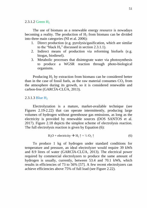
2.3.1.3 Blue H2
Electrolyzation is a mature, market-available technique (see
Figures 2.19-2.22) that can operate intermittently, producing large
volumes of hydrogen without greenhouse gas emissions, as long as the
electricity is provided by renewable sources (DOS SANTOS et al.
2017). Figure 2.18 depicts the simplest scheme of electrolysis reaction.
The full electrolysis reaction is given by Equation (6):
H2O + electricity H2 ↑ + ½ O2 ↑ (6)
To produce 1 kg of hydrogen under standard conditions for
temperature and pressure, an ideal electrolyzer would require 39 kWh
and 8.9 litres of water (GARCÍA-CLÚA, 2013). The electrical power
required by commercial electrolyzers to produce the same amount of
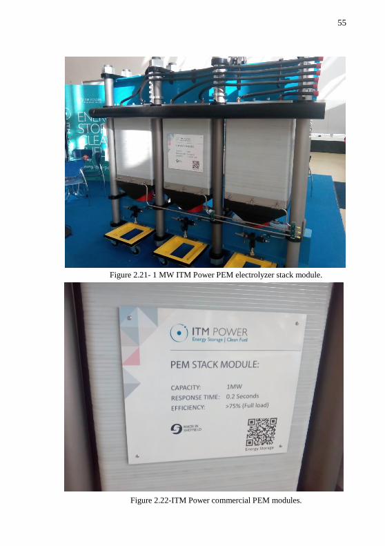
hydrogen is usually, currently, between 53.4 and 70.1 kWh, which
results in efficiencies of 73 to 56% [57]. A few recent electrolyzers can
achieve efficiencies above 75% of full load (see Figure 2.22).
Page 58
52
Figure 2.19- Scheme of the electrolysis reaction
(http://www.diracdelta.co.uk/science/source/w/a/water%20electrolysis/source.html#.
WJHVNH_iSyI).
There are two main types of low temperature electrolyzers: alkaline
(GANLEY, 2009) and proton exchange membrane, PEM (BARBIR,
2005), which are the most frequent in the market. Furthermore, there
exist high temperature electrolyzers (SOEC), but they are still only a
promising technology (SCHILLER et al. 2009).
Alkaline electrolysis
Alkaline electrolyzers generate H2 with a purity better than
99.97%, which is the quality used in the automotive industry
(PETERSEN, 2012). They are already available at the power levels
(about MW) that make the technology cost-efficient (see Refs
(VALVERDE et al. 2016), (RASHID et al. 2015), (MORGAN et al.
2013) and (XIANG et al. 2016) for details). An aqueous solution of 20
to 30% potassium hydroxide (KOH) is used as the ionically conductive
medium. The electrodes immersed in this electrolyte are polarized by
electrochemical reactions (7) and (8), resulting in the overall reaction (6)
presented before:
Cathode 2H2O + 2e- H2 ↑ + 2OH
- (7)
Anode 2OH- ½ O2 ↑ + H2O + 2e
- (8)
Page 59
53
Each cathode-anode pair forms a basic electrolysis cell that
operates at 1.9-2.5V DC. There are two types of cell design: unipolar
and bipolar. Unipolar cells are interconnected in parallel by single
polarity electrodes. In this way, high currents and low voltages are
obtained. Unipolar cells are simpler to repair than bipolar. Bipolar cells
are interconnected in series leading to higher battery voltages, thus,
electrodes assume both polarities. Each of the electrodes acts as an
anode on one face and as a cathode on the other, except those located at
the ends. The stack is connected via alternating layers of electrodes with
separation membranes and compressing the assembly with clamps. As
cells are relatively thin, the entire stack can be considerably smaller than
in the unipolar design. One disadvantage is that a cell cannot be repaired
without removing the entire stack. The main challenges for the future of
alkaline electrolysis are reducing costs and increasing energy efficiency
(GARCÍA-CLÚA, 2013). Figure 2.20 presents a bipolar design of an
alkaline electrolyzer stack.
Figure 2.20-Alkaline electrolyzer stack filled with a KOH pure solution
(http://www.alnooroils.com/en/post.php?id=26).
Page 60
54
PEM Electrolysis
A second electrolyzer technology that is commercially available is
the solid Polymer Electrolyte Membrane, or PEM. In a PEM
electrolyzer, the electrolyte is in a thin, solid, ion-conducting membrane
instead of the aqueous solution of alkaline electrolyzers. This allows
protons to transfer from the anode to the cathode and, in this way, H2
can be separated from O2 (GARCÍA-CLÚA, 2013). PEM electrolyzers
have advantages in terms of safety when compared with alternative
technologies (see (MANSILLA et al. 2013) and references therein);
moreover, they have already been successfully tested in marine
environments (DI BLASI et al 2013). Hydrogen is produced at the
cathode side and oxygen on the anode side, following reactions (9) and
(10). In the case of an acidic PEM cell, it is assumed that liquid water
splitting occurs according to the following half-cell reactions:
Cathode 2H
+ + 2e
- H2 ↑ (9)
Anode H2O ½ O2 ↑ + 2H+ + 2e
- (10)
Solvated protons formed at the oxygen-evolving anode of the PEM
cell migrate through the membrane to the cathode, where they are
reduced to molecular hydrogen. PEM technology is one of the most
promising water electrolysis technologies for direct coupling with
renewable electrical sources (ROZAIN et al: 2016, MENDES et al.
2016). Figures 2.21 and 2.22, respectively, show a PEM module and
stack.
High temperature electrolysis
Solid Oxide Electrolyzer Cells (SOECs) have attracted a great deal
of interest because they can convert electrical energy into chemical
energy, producing hydrogen with high efficiency (CARMO et al. 2013).
In 1985, Dönitz and Erdle were the first to report results from a solid
oxide electrolyzer (SOECs) using a supported tubular electrolyte.
Nowadays, preliminary lab-scale studies are mainly focused on the
development of novel, improved, low cost and highly durable materials
for SOECs.
Page 61
55
Figure 2.21- 1 MW ITM Power PEM electrolyzer stack module.
Figure 2.22-ITM Power commercial PEM modules.
Page 62
56
These studies focus on the development of the inherent
manufacturing processes, and the integration in efficient and durable
electrolyzers. Also interesting is the fact that SOECs could be used for
the electrolysis of CO2 to CO, and also for the co-electrolysis of
H2O/CO2 to H2/CO (syngas) (CARMO et al. 2013). The SOEC
technology is still a promising technology, but has a huge potential for
the future mass production of H2, if the issues related to operation and
durability of the ceramic materials at high temperature are solved
(REITER, 2016).
2.4 MODEL PREDICTIVE CONTROL
The term Model Predictive Control (MPC) does not designate a
specific control strategy, but a very ample range of control methods
which make explicit use of a model of the process to obtain the control
signal by minimizing an objective function. Three decades have passed
since milestone publications by several industrialists spawned a flurry of
research and industrial/commercial activities on MPC (LEE, 2011). This
control system has been popular in industry since the 1980s and there is
steadily increasing attention from control practitioners and theoreticians
(CAMACHO; BORDONS, 2013). Throughout the three decades of the
development, theory and practice supported each other quite effectively,
a primary reason for the fast and steady rise of the technology (LEE,
2011). MPC was originally studied and applied in the process industry,
where it has been in use for decades (MORARI; LEE, 1999). Now,
predictive control is being considered in other areas, such as power
electronics and drives (RODRIGUEZ et al. 2013). The reason for the
growing interest in the use of MPC in this field is the existence of very
good mathematical models to predict the behaviour of the variables
under control in electrical and mechanical systems (VAZQUEZ et al.
2014). Comparing with other methods of process control, MPC can be
used to solve the most common problems in today's industrial processes,
which need to be operated under tight performance specifications where
many constraints need to be satisfied (CHRISTOFIDES et al. 2013).
2.4.1 MPC strategy
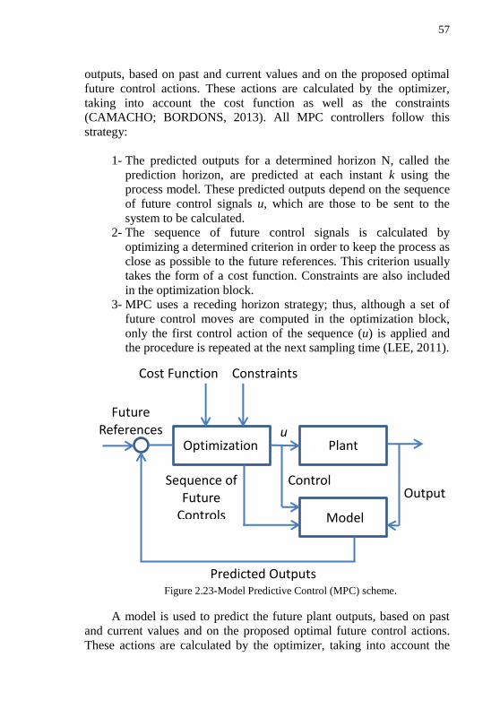
The principal elements in MPC are shown in Figure 2.23. The
main characteristic is the use of the model of the system for the
prediction of the future behaviour of the controlled variables
(VAZQUEZ et al. 2014). This model is used to predict the future plant
Page 63
57
outputs, based on past and current values and on the proposed optimal
future control actions. These actions are calculated by the optimizer,
taking into account the cost function as well as the constraints
(CAMACHO; BORDONS, 2013). All MPC controllers follow this
strategy:
1- The predicted outputs for a determined horizon N, called the
prediction horizon, are predicted at each instant k using the
process model. These predicted outputs depend on the sequence
of future control signals u, which are those to be sent to the
system to be calculated.
2- The sequence of future control signals is calculated by
optimizing a determined criterion in order to keep the process as
close as possible to the future references. This criterion usually
takes the form of a cost function. Constraints are also included
in the optimization block.
3- MPC uses a receding horizon strategy; thus, although a set of
future control moves are computed in the optimization block,
only the first control action of the sequence (u) is applied and
the procedure is repeated at the next sampling time (LEE, 2011).
Figure 2.23-Model Predictive Control (MPC) scheme.
A model is used to predict the future plant outputs, based on past
and current values and on the proposed optimal future control actions.
These actions are calculated by the optimizer, taking into account the
Output
Optimization Plant
Model
Future References
Constraints Cost Function
u
Sequence of Future
Controls
Predicted Outputs
Control
Page 64
58
cost function (where the future tracking error is considered) as well as
the constraints. The process model consequently plays a decisive role in
the controller. The chosen model must be capable of capturing the
process dynamics so as to precisely predict the future outputs, as well as
being simple to implement and to understand. The optimizer is another
fundamental part of the strategy as it provides the control actions
(CAMACHO; BORDONS, 2013).
2.4.2 Receding horizon
It is important to remark that one of the most important
characteristics of the MPC is the use of the receding horizon. At each
instant, the horizon is displaced towards the future, which involves the
application of the sequence calculated at each step k. In this type of
strategy, only the first control actions are taken at each instant and the
procedure is again repeated for the next control decisions in a receding
horizon fashion (unlike other classical control schemes such as PIDs, in
which the control actions are taken based on past errors). In the
receding-horizon strategy, only the first elements of the control variable
are used, rejecting the rest and repeating the calculations at the next
sampling time (CAMACHO; BORDONS, 2013).
Figure 2.24-Receding horizon scheme (PARASCHIV et al. 2009).
Page 65
59
2.4.3 Constraints
To solve MPC constraints in this thesis, the Mixed Logical
Dynamical System (MLD) will be used. The MLD was developed for
the first time by (BEMPORAD; MORARI, 1999) to associate the
performance of the system with discrete variables δ and continuous
variables α. MLD conversions make it possible to include binary and
auxiliary variables, introduced in a discrete-time dynamic system to
describe, in a unified model, the evolution of the continuous and logic
signals of the system.
The MLD MPC results in an optimization problem with a set of
linear constraints and integer (in this case Boolean) decision variables.
With the introduction of a series of basic conversions, given in Table
1.1, the non-linearity of the system, introduced by the combination of
logical and dynamic variables, is transformed into constraints of the
control algorithm (GARCÍA-TORRES, 2015). In Table 1.1, m and M
represent the lower and upper bounds of the system and ε > 0 is the
smaller tolerance of the device (BEMPORAD; MORARI, 1999).
Relation Logic MLD Inequalities
P1 AND (˄) S1 ˄ S2 δ1 = 1, δ2 = 1 P2
S3 ↔ (S1 ˄ S2) -δ1 + δ3 ≤ 0 -δ2 + δ3 ≤ 0
δ1 + δ2 – δ3 ≤ 1 P3 OR (˅) S1 ˅ S2 δ1 + δ2 ≥ 1 P4 NOT (~) ~ S1 δ1 = 0 P5 IMPLY (→) S1 → S2 -δ1 - δ2 ≤ 0 P6 IF (↔) S1 ↔ S2 -δ1 - δ2 = 0 P7 [aTx ≤ 0] → [δ = 1] aTx ≥ ε + (m - ε) P8 [δ = 1] → [aTx ≤ 0] aT ≤ M - Mδ P9
[aTx ≤ 0] ↔ [δ = 1] aT ≤ M – Mδ
aT ≥ ε + (m - ε) δ P10
Mixed Product
z = δ∙aTx
z ≤ Mδ z ≥ mδ
z ≤ aTx – m(1- δ) z ≥ aTx – M(1- δ)
Table 1.1 – Conversion of logic relations into Mixed Integer Inequalities.
Page 66
60
2.5 CONTRIBUTIONS OF THE THESIS
2.5.1 Journal papers
SERNA, A.; YAHYAOUI, I.; NORMEY-RICO, J. E.; de PRADA, C.;
TADEO, F. Predictive control for hydrogen production by electrolysis
in an offshore platform using renewable energies. International
Journal of Hydrogen Energy, 42(17) 12865-12876, 2017. IF (2016):
3.6.
SERNA, A.; TADEO, F.; NORMEY-RICO, J. E. Ruled-based control
of off-grid desalination powered by renewable energies. Renewable
energy and sustainable development, pp 205-213, 1, No1, 2015.
SERNA, A.; TADEO, F. Offshore hydrogen production from wave
energy. International Journal of Hydrogen Energy, 39(3), 1549-
1557, 2014. IF (2014): 3.3.
SERNA, A.; TADEO, F. Offshore desalination using wave energy.
Advances in Mechanical Engineering, 5, 539857, 2013. IF (2013):
0.5.
2.5.2 Conference papers
SERNA, A.; TADEO, F.; YAHYAOUI, I.; NORMEY-RICO, J. E.
Business background analysis for a controlled hydrogen-based
microgrid. In Proceedings of the 14th
International Workshop on
Advanced Control and Diagnosis (ACD), November 2017,
Bucharest, Romania.
SERNA, A.; TADEO, F.; NORMEY-RICO, J.E. Advanced control
based on MPC ideas for offshore hydrogen production. In Proceedings
of the 38th
Jornadas de Automática 2017, September, Gijón, Spain.
SERNA, A.; TADEO, F.; YAHYAOUI, I.; NORMEY-RICO, J. E.;
GARCIA-TORRES, F. Evaluation of a Long Term System coupled with
a Short Term System of a Hydrogen-Based Microgrid. In Proceedings of
the 8th
International Renewable Energy Congress (IREC), March
2017, Amman, Jordan. (pp. 1-6). IEEE.
Page 67
61
SERNA, A.; TADEO, F.; NORMEY-RICO, J. E.; AGERSTED, K.
Ruled-based control of off-grid electrolysis. In Proceedings of the 21st
World Hydrogen Energy Congress (WHEC), June 2016, Zaragoza,
Spain.
SERNA, A.; TADEO, F.; NORMEY-RICO, J. E. Mixed-Integer-
Quadratic-Programming based Predictive Control for hydrogen
production using renewable energy. In Proceedings of the 7th
International Renewable Energy Congress (IREC), March 2016,
Hammamet, Tunisia. (pp. 1-6). IEEE.
SERNA, A.; TADEO, F.; NORMEY-RICO, J. E. Control avanzado
basado en ideas de control predictivo para la producción de hidrógeno
mediante electrólisis. In Proceedings of the 14th
Simposio de Ingeniería
de Control CEA 2016, March 2016, Logroño, Spain.
SERNA, A.; TADEO, F.; NORMEY-RICO, J.E. Producción de
hidrógeno por energías renovables en una plataforma híbrida en alta
mar. In Proceedings of the 36th
Jornadas de Automática 2015,
September, Bilbao, Spain.
SERNA, A.; NORMEY-RICO, J. E.; TADEO, F. Model predictive
control of hydrogen production by renewable energy. In Proceedings of
the 6th
International Renewable Energy Congress (IREC), March
2015, Sousse, Tunisia. (pp. 1-6). IEEE.
SERNA, A.; TADEO, F.; TORRIJOS, D. Heuristic control of multi-
stage desalination plants under variable available power. In Proceedings
of the 15th
International Conference of Sciences and Techniques of
Automatic Control and Computer Engineering (STA), December
2014, Hammamet, Tunisia. (pp. 853-858). IEEE.
SERNA, A.; TORRIJOS, D.; TADEO, F., TOUATI, K. Evaluation of
wave energy for a near-the-coast offshore desalination plant. In
Proceedings of the International Desalination Association (IDA)
World Congress, October 2013, Tianjin, China.
2.5.3 Other contributions
Co-author of one chapter in the book titled “Advances in Renewable
Energies and Power Technologies: Volume 1: Solar and Wind Energy”
Page 68
62
ISBN: 9780128129593 and one chapter in the book titled: “Advances in
Renewable Energies and Power Technologies: Volume 2: Geothermal
and Biomass Energies, Fuel Cells and Smart Grids” ISBN:
9780128131855. Edited by Dr. Imene Yahyaoui. Elsevier, 1st January
2018.
YAHYAOUI, I.; ATIEH, A.; SERNA, A.; TADEO, F. Sensitivity
analysis for photovoltaic water pumping systems: Energetic and
economic studies. Energy Conversion and Management, 135, 402-
415, 2017. IF (2016): 5.6.
SERNA, A.; TADEO, F.; NORMEY-RICO, J. E. Control de la
producción de H2 por energías renovables en una plataforma híbrida en
alta mar. In the 3rd
Jornadas del Programa de Doctorandos de la
Universidad de Valladolid, September 2016, Valladolid, Spain. Poster presentation.
SERNA, A.; TADEO, F.; NORMEY-RICO, J.E. (2015, March).
Sistema de control en la producción de hidrógeno en alta mar mediante
energías renovables. In the 8th
Reunión de Jóvenes Investigadores
Iberoamericanos, March 2015, Tordesillas, Spain. Poster
presentation.
SERNA, A.; TADEO, F. Modelling of an offshore hydrogen production
from wave energy. In Proceedings of the 4th
International Renewable
Energy Congress (IREC), December 2012, Sousse, Tunisia. Oral
presentation.
SERNA, A.; TADEO, F.; de PRADA, C. The H2OCEAN Project: A
wind + wave power open-sea platform equipped for hydrogen
generation. In Offshore Wind Turbines Workshop, University of
Hull, September 2012, Hull, UK. Poster presentation.
2.5.4 Patent and intellectual property registration
Title: Offshore hydrogen production using wave energy
Author: ÁLVARO SERNA CANTERO
Reference number: VA-299-2013
Year: 2013
Right holder: University of Valladolid (Spain)
Page 69
63
Winner of the University of Valladolid “Prometeo” award 2013
whose aim is the stimulation of the application of knowledge, as well as
collaboration between knowledge-generating agents and specialists in
the transfer of knowledge and the promotion of a culture of innovation
and creativity. For this, this award provides incentives for the
development of market-oriented prototypes, achieving a set of products
that can be offered to meet the needs of the market.
2.6 ORGANIZATION OF THE THESIS
This thesis is organized as follows:
Chapter 1: This chapter introduces the thesis content. Section 1.1
gives the motivation, while section 1.2 give details of the objectives
proposed for this thesis.
Chapter 2: This chapter deals with the state of the art of the
technologies developed in the thesis. Section 2.1 is dedicated to
renewable energies. Section 2.2 gives a review of reverse osmosis.
Section 2.3 presents information about hydrogen economy and
production, followed by a summary of Model Predictive Control theory
(Section 2.4). Finally, the contributions of the thesis are detailed.
Chapter 3: This chapter focuses on the design of control strategies
for the production of water by Reverse Osmosis and hydrogen by
electrolysis within the H2OCEAN offshore platform. Section 3.1 is
dedicated to the fresh water production, whilst Section 3.2 deals with
hydrogen production. Finally, this chapter ends with some conclusions.
Chapter 4: This chapter develops an Energy Management System
of hydrogen production (EMSH) based on Model Predictive Control
ideas optimizing the connections and disconnections of the
electrolyzers. This numerical optimization solves a Mixed-Integer
Quadratic Programming algorithm with constraints.
Chapter 5: This chapter comprises the coupling of a short-term control system with the long-term EMSH proposed in Chapter 4 for a
hydrogen-based microgrid composed of electrolyzers, battery and an
ultracapacitor.
Page 70
64
Chapter 6: This chapter includes some conclusions and future
work.
Annex: This annex presents an economic study and a business
plan for the hydrogen-based microgrid proposed in Chapter 5.
2.7 SUMMARY AND CONCLUSIONS
In this chapter, an overall introduction of the technologies
developed in the thesis has been detailed:
Wind and wave energy are the energy sources chosen to produce
energy, as they can be easily obtained in the H2OCEAN platform.
Reverse Osmosis is the most adequate technology to transform
seawater into fresh water. It is very well known and commercially
available.
Electrolysis has been chosen to obtain hydrogen from water due to
its technological maturity and easy implementation.
Model Predictive Control is an advanced control strategy that can
be used to solve the most common problems in today's industrial
processes, which need to be operated under tight performance
specifications. Thus, it was chosen to design the Energy
Management System for hydrogen production that is fully
developed in Chapter 4.
The chapter ended with the contributions made by the author
during the thesis and the organization of the different chapters.
Page 71
65
CHAPTER 3
CONTROL OF THE H2OCEAN
PLATFORM
Page 73
67
3 CONTROL PROPOSAL FOR THE H2OCEAN PLATFORM
This chapter deals with the design of control strategies for the
production of water by Reverse Osmosis (RO) and hydrogen by
electrolysis in the renewable energy offshore H2OCEAN platform. The
purpose is to test the feasibility of these control systems in the
production of drinkable water and hydrogen using renewable energy in
out-of-sight installations. These tasks were defined in Section 1.1 as part
of the work done by the University of Valladolid for the H2OCEAN
project.
3.1 FRESH H2O PRODUCTION IN THE H2OCEAN PLATFORM
This section evaluates a control proposal design for water
production within the H2OCEAN project (see Section 1.1), which will
be evaluated for two different case studies.
First, the subsystems that compose the proposed desalination plant
are described. Then, for the first case study, an Energy Management
System for Water production (EMSW) based on heuristic control is
given, as well as a proposal for sizing these subsystems. The influence
of sizing on the expected performance is then studied for a specific
location using buoy-measured data.
Finally a second case study proposes a rule-based EMSW to control
the installation, due to its easier implementation so that low conductivity
water for electrolysis can be produced. This case study is also evaluated
using buoy-measured data.
The proposal presented here is based on dividing the desalination
plant into a few sections, which would be switched on or shutdown,
depending on the available energy (SERNA; TADEO, 2013). All of this
requires an EMSW which be will discussed later. Power consumption
adapts to power production by connecting or disconnecting sections of
the installation (following a Smart Grid approach for the microgrid in
the plant). The temporary storage of electricity in batteries for short-time
balances is selected for its smooth operation and for the increase in
autonomy.
A description of the different components of the desalination plant
is given in 3.1.1, whilst the first case study is proposed in section 3.1.2.
The second case study is presented in section 3.1.3.
Page 74
68
3.1.1 Desalination plant operation
The process diagram in Figure 3.1 presents the main blocks of the
proposal: the renewable energy sources, the supply of seawater through
seawater pumps (SWP) and the desalination stage. A set of batteries
provide electricity for the case of there being no renewable energy
available. Then, fresh water is transported (by tankers, bladders or
pipes) to the hydrogen production section.
As already mentioned in Section 2.1, renewable energy production
changes over time, which requires the production of water (and thus
power consumption) to be adapted to the available power. This is
challenging for RO plants, as they are normally designed to operate at
an optimal working point. Changing the working point of the plant (thus
changing the flow/pressure combination from a specific value) makes it
possible to adapt the RO electrical load to the demand.
Figure 3.1 - Structure of the proposed desalination installation
A specific EMSW, discussed later, would be responsible for
adapting power consumption to demand, always with the aim of
operating the plant at the best possible overall efficiency, while taking
into account the operating constraints.
3.1.2 First case study
The desalination plant proposed in this section was developed as part of the H2OCEAN project (SERNA; TADEO, 2013) from previous
designs by SETA (Sociedad Española de Tratamiento de Agua). It is
shown in Figure 3.2.
In this first case study the first proposal of EMSW is developed. It
was decided to partition the desalination stage of the RO plant into three
Seawater Supply (SWP)
Batteries
Desalination Stage
Renewable Energy
Seawater
Fresh Water
Seawater
Local Microgrid
Page 75
69
sections of different sizes (A, B and C): the three sections operate as a
standard RO plant (producing water with maximum efficiency, at a
fixed working point). Sections can operate on an individual basis or
together with other sections, depending on the available energy.
Seawater with flow QS is taken from the sea by the SWPs before
being stored in a single seawater tank with volume VS, as can be seen in
Figure 3.2. It is then desalinated and stored in a fresh water tank with
volume BT1, in order to transport it offshore through pipes and/or water
tank ships or bladders (represented by flow QF).
A Section (RO)A Section (RO)
Flow (A) = 150 m3/h
B Section (RO)B Section (RO)
C Section (RO)C Section (RO)
Flow (B) = 70 m3/h
Flow (C) = 40 m3/hSWP 1
SWP 2
SWP 3
Seawater supply Desalination
Seawater tank
(Vs)Fresh water tank
(BT1)
80 m3/h45 kW
80 m3/h45 kW
80 m3/h45 kW
95 kW
150 kW
340 kW
FWP C
FWP B
FWP A
Fresh water
(QF)
Seawater
(Qs)
Figure 3.2 - Structure of the first case study.
The proposed system is off-grid, so energy production and demand
must be balanced. Several technologies have been proposed for temporary storage (ANTONIA; SAUR, 2012). Here, we propose the
following EMSW for this first case study:
Page 76
70
3.1.2.1 Energy Management System based on heuristic control
A central component to ensure the smooth operation of the facility
is the control system, which should balance electricity production and
consumption by adapting the consumed loads: the power of the seawater
pumps (SWPs) and the high pressure pumps working in the different
sections of the RO.
The key decision variable, the Depth of Discharge (DOD) of a
battery, is the percentage of capacity to which it is discharged. Values
approaching 1 correspond to the battery being almost discharged. It is
assumed that the control algorithm is based on the two following ideas:
1) Main control variables are the connection/disconnection of the
different sections A, B and C in the RO and the SWPs (See
Figure 3.3).
- When the production is higher than the consumption, the energy
is stored so the DOD of the battery decreases: until the temporary
storage system is nearly full, different sections of the RO and the
SWP are switched on depending on the value of the DOD.
- If the DOD increases significantly because production is lower
than demand, sections of the RO and the SWP are switched off
(these sections are then automatically cleaned and maintenance
operations are carried out).
2) Another control variable is the connection/disconnection of the
three SWPs for safety conditions, as these pumps operate
independently from the RO plant:
- When the level of the seawater tank VS is higher than a certain
safety value (LT≥LTmax), the three SWPs are switched off
simultaneously.
- When the level of the seawater tank VS is lower than a certain
safety value (L≤LTmin), the three SWPs are switched on
simultaneously.
Page 77
71
Control System
Produced Energy
swit
ch o
n/o
ff
Sect
ion
A
swit
ch o
n/o
ff S
WP
1
swit
ch o
n/o
ff
Sect
ion
B
Reverse Osmosis
Plant
Legend: integer variable
swit
ch o
n/o
ff
Sect
ion
C
swit
ch o
n/o
ff S
WP
2
swit
ch o
n/o
ff S
WP
3
continuous variable
Seawater Supply
Battery DOD
Figure 3.3- Proposed EMSW for the first case study
The control logic is summarized in the Sequential Function Chart
in Figure 3.4, where different sequences of the desalination process can
be seen. There is one different combination of RO sections (A, B and C)
in each stage. Therefore, for each range of DOD values, there is a
certain operating stage. Furthermore, in each stage, the three SWPs are
switched on/off one by one depending on the value of the DOD, as can
Page 78
72
be seen in the detail of the Sequential Function Chart of stage A
presented in Figure 3.5.
Idle
B
C+B
A
A+C
A+B
A+B+C
DOD ≤ 0.45
DOD ≤ 0.3
DOD ≤ 0.2
DOD ≤ 0.05
DOD ≥ 0.2
DOD ≥ 0.25
DOD ≥ 0.35
DOD ≥ 0.5
DOD ≥ 0.65
DOD ≥ 0.85
DOD ≤ 0.8
DOD ≤ 0.6
Figure 3.4 - Sequential Function Chart of the Control Logic of the RO
Page 79
73
A.0No
Pump
A.1SWP1
A.2SWP1+2
A.3SWP1+2+3
DOD ≥ 0.35
DOD ≥ 0.4
L ≤ Lmin
L ≤ Lmax AND DOD ≤ 0.3
L ≤ Lmax AND DOD ≤ 0.35
L ≤ Lmax AND DOD ≤ 0.4
L ≤ Lmax AND DOD ≤ 0.45
To A+C
From C+B or A+C
DOD ≥ 0.5
To C+B
Stage A
A.0 A.1 A.2
A.1 A.2 A.3
L ≥ Lmax
Figure 3.5 - Detail of the Sequential Function Chart (Stage A)
For this case study, a standard Pb battery rack system is assumed,
as it has wide experience in marine applications. During charge, the
electrons are provided by an external power source. The nominal
voltage of the lead-acid cell is 2 volts (SZYMBORSKI, 2002). The
batteries are used to provide energy to the reverse osmosis plant and the
SWPs when not enough power is provided by the renewable energies.
I =PW−PT
V (11)
where I is the amperage of the battery, V is the voltage, Pw is the
power supplied by renewable energies, and PT is the total power
consumed by the SWP and the RO. The equation relating the capacity of
the battery and the amperage is as follows (SERNA; TADEO, 2013):
Page 80
74
dCR
dt= ψ
IkP
3600 (12)
where CR is the rated capacity at that discharge rate, t is the time,
kP is Peukert´s coefficient, and ψ is the efficiency of the battery. The
DOD is given by the expression below, where CP is Peukert´s capacity.
DOD = 1 −CR
CP (13)
The value of the % of battery charge is given by this simple
equation:
% Battery charge = (1 − DOD) ∙ 100 (14)
The DOD is used in more works (YAHYAOUI et al. 2014) to
control different devices, such as photovoltaic panels or batteries. It is
important to note the importance of the fact that the constant discharging
and charging of the batteries often leads to them becoming quickly
ineffective. Therefore, the battery capacity finally chosen for the
simulation in Section 3.1.2.3 aims to be the least harmful to the system.
3.1.2.2 Sizing of the first case study
In the proposed facility shown in Fig. 3.2, a central aspect of the
design for a specific location is the selection of the size of the
components, so as to ensure the autonomous operation of the facility
without excessive capital or operation costs. In particular, the following
parameters should be selected:
The maximum fresh water demand, QF (m3/h).
The total rated power consumption of the process, PT (kW).
The volume of the seawater tank, VS (m3).
The battery capacity, CP (Ah).
In this kind of renewable energy installations, it is important to
consider the variability of the source: thus, forecasts are usually needed
(LEI et al. 2009). In this case, we assume that a significant record of
data measured in the location where the Wave Energy Converters
(WECs) and Vertical Axis Wind Turbines (VAWTs) would be placed is
Page 81
75
available. The sizing of the proposed facility can be carried out on the
basis of the measured data. The proposed methodology to select the
plant parameters is then the following:
1) Using the measured data, the evolution of the power produced by
the renewable energy devices, PW (t), is estimated as explained in
Sections 2.1.1 and 2.1.2.
2) The total rated power consumption of the process PT is selected to
ensure that one or more of the different sections of the RO operate
for at least some of the time. This value must always be less than
PW.
3) The tank size VS is selected to ensure autonomy at all times (LTmin
≤ L ≤ LTmax).
4) The battery capacity CP is selected to ensure Wa hours of autonomy
at idle of all times and that the DOD is always between given
limits DOD < DOD < DOD.
Figure 3.6 shows inputs and outputs in the sizing scheme, taking into
account the variables of the desalination installation:
Figure 3.6 - Scheme of the sizing for the first case study
3.1.2.3 Results and discussion
The first case study proposes a desalination stage designed to
operate consuming between 95 kW and 585 kW of electricity (PT) as
shown in Fig. 3.2: section A is designed to produce 150 m3/h with a
consumption of 340 kW, whereas section B is designed to produce 70
m3/h with a consumption of 150 kW, and C produces 40 m
3/h
consuming 95 kW. The energy consumption of the RO units (power
consumed between water produced) is about 2.4 kWh/m3 and the plant
PT
QF
Wa
CP
VS RO
INSTALLATION
Page 82
76
recovery ratio (water input between water output) is about 50%
(SERNA; TADEO, 2013).
There are three seawater pumps (SWPs) that provide water from
the seawater intake to the seawater tank. Each pump works with a power
of 45 kW and a flow rate of 80 m3/h. These pumps are on-off pumps that
work (or not) while the tank level is between certain values: if the tank
level is higher than a safety value, all the pumps immediately switch off.
Thus, the tank level can be controlled as has been detailed in Figure 3.5.
To validate the proposed offshore platform and the sizing
methodology, this case study was carried out for a specific location in
the Atlantic Ocean, selected for its good wave regime. For this location,
buoy data was measured for 165 days (wind speed, wave heights, wave
periods, water salinity and temperature, etc.). Based on this data, an
installation was designed using the proposed sizing methodology. This
design was then tested assuming different platform parameters. The
simulation was modelled and performed using MATLAB® and
Simulink®.
Figure 3.7 shows the effect of the battery’s capacity on system
performance: the RO plant capacity and switch on-off times of the
SWPs and sections of the RO for a tank volume (VS) of 5500 m3. It also
shows that the amount of fresh water produced (QF) increases until a
battery capacity value of CP = 2400 Ah, remaining constant after this
value. The value of the number of times that the SWPs are switched on-
off is independent of the battery capacity. The number of times that the
RO is switched on-off decreases with the increase in the battery’s
capacity. Therefore, a battery capacity of 2400 Ah will be chosen to
evaluate the effect of the seawater tank size on system performance.
Figure 3.8 shows the effect of the seawater tank volume with the
same system parameters for the case of a battery capacity of 2400 Ah. It
also shows that the amount of fresh water produced, QF, is independent
of the seawater tank volume VS. The same behaviour has been seen with
the number of times that the sections of the RO are switched on-off. The
value of the number of times that the SWP are switched on-off decreases
in line with the tank volume VS. Thus, a volume of 7700 m3 it has been
chosen
Page 83
77
Figure 3.7 - Effect of battery capacity (CP) on system performance (VS = 5500 m3).
Figure 3.8 - Effect of seawater tank volume (VS) on system performance (CP = 2400
Ah).
0
10
20
30
40
50
60
70
80
90
100
101
102
103
104
105
106
107
108
109
110
0 1000 2000 3000
On
-Off
SW
P/R
O
Fre
sh w
ate
r (Q
F) 1∙1
03 m
3 /m
on
th
Battery capacity (Ah)
Water produced (m3/month)
On-Off SWP
On-Off RO
2400
0
5
10
15
20
25
30
100
101
102
103
104
105
106
107
108
109
110
0 5000 10000
On
-Off
SW
P/R
O
Fre
sh w
ate
r (Q
F) 1∙10
3m
3 /m
on
th
Tank volume (m3)
Water produced m3/month
On-Off SWP
On-Off RO
7700
Page 84
78
Finally, an operating point was selected (in bold), which is the first
presented in Table 3.1.
Battery capacity
(Ah)
Tank volume
(m3)
Fresh water (m
3/month)
On-Off SWP
(times/month) On-Off RO
(times/month)
2400 7700 106693 4.8 20.6
2400 5500 105860 8.2 19.8 1000 5500 103128 4.8 16.4
Table 3.1 - Selected operating point for the first case study
Figures 3.9 to 3.14 show different parameters at the operating point
on 165 days with buoy measurements. It can be seen that the proposed
system operates adequately:
Figure 3.9 represents the power produced by the renewable energy
sources (PW). The power produced depends on the values of the wave´s
height and period and on the wind speed.
Figure 3.10 shows that the value of the fresh water produced in
each RO section varies over time, according to the activation of the
stages of the RO illustrated in Figure 3.2.
Figure 3.11 shows the total fresh water produced (QF), which is the
sum of sections A, B and C. It can be seen that this value increases if the
value of the power produced (Figure 3.9) is high.
Figure 3.12 depicts the total power consumed, PT. This is
proportional to the total fresh water produced plus the power consumed
by the SWPs.
Figure 3.13 shows the stored seawater. The value is between the
minimum and maximum safety level.
Finally, Figure 3.14 depicts the value of the % Battery charge. As
expected, this value varies between 30% and 100%, so it never gets
discharged.
Figure 3.9 - Power produced by renewable energies (Pw)
0 20 40 60 80 100 120 140 160 0
500
1000
1500
Time (days)
Pow
er
pro
duce
d (
kW
)
Page 85
79
Figure 3.10- Fresh water produced (QF) in each RO section
Figure 3.11- Total fresh water produced (QF)
Figure 3.12 - Total power consumed (PT)
Figure 3.13 - Stored seawater
0 20 40 60 80 100 120 140 160 0
50
100
150
Time (days)
Flo
w r
ate
(m
3/h
)
Section A Section B Section C
0 20 40 60 80 100 120 140 160 0
50
100
150
200
250
300
Time (days)
Flo
w r
ate
(m
3/h
)
0 20 40 60 80 100 120 140 160 0
200
400
600
800
Time (days)
Pow
er
co
nsum
ed (
kW
)
0 20 40 60 80 100 120 140 160 0
2000
4000
6000
8000
Time (days)
Sto
red s
ea
wate
r (m
3)
Page 86
80
Figure 3.14 - % Battery charge: 100% (1-DOD).
3.1.3 Second case study
The approach presented in Section 3.1.2 is developed for
desalination plants with few sections. However, it is not adequate when
there is a significant number of units being used and complex control
objectives; in particular, it is not adequate for multi-stage desalination
plants operated by several lines, as the number of components with high
electrical consumptions (high pressure pumps) is too big to develop and
maintain a functional block diagram that accurately represents the
control objectives.
In fact, water for electrolysis requires low conductivity (few
µS/cm); therefore, the H2OCEAN desalination section is composed of
two successive stages, solving complex control objectives.
Thus, an alternative procedure is presented in this section which
combines the implementation in existing control hardware (PLCs) with
the fulfilment of conflicting control objectives.
In this second case study, a ruled-based control strategy is
porposed for a reverse osmosis plant powered by renewable energy
which is simple to implement and, as will be shown, presents good
results (SERNA et al. 2015). There are some previous works that use
rule-based control strategies for energy management: JALIL et al.
(1997) designed a rule-based control for a hybrid vehicle, whilst PARIS
et al. (2010) developed this control strategy in the design of heating
control schemes for energy management in buildings.
3.1.3.1 Energy Management System for the second case study
For the sake of simplicity, the control proposal is presented for a
platform with a single seawater pump, two high pressure pumps for a
first stage of RO and two high pressure pumps for a second stage, as can
be seen in Figure 3.15.
0 20 40 60 80 100 120 140 160 0
20
40
60
80
100
Time (days)
% B
atte
ry c
ha
rge
Page 87
81
The characteristics of each of the units of consumption are as
follows (SERNA; TADEO, 2015):
• A 51 kW SWP that provides a nominal flow rate of 256 m3/h (QS).
• The first stage of the RO plant, RO1, consists of two similar lines,
each designed to produce 57 m3/h (QF) of fresh water when
connected (with a recovery ratio of around 45%), consuming 155
kW per line (corresponding to approximately 2.7 kWh/m3) when
they are operating.
• The second stage, RO2, also consists of two similar lines, which,
when connected, produce 34 m3/h (QDE) of demineralized water
(recovery ratio of 75%), in each line, consuming around 38 kW per
line (approximately 1 kWh/m3 of demineralized water produced).
Figure 3.15 - Structure of the second case study
Parallel approaches can be easily extended for other configurations, perhaps using other components with different rated
powers and configurations. The main goal to ensure the smooth
operation of the facility is the control system, balancing power
consumption with the available power by deciding which units of the
QDE QF
HP2B
38kW
DEMI Water Tank BT2
(148 m3)
RO1A
RO1B
RO2A
RO2B
Seawater Intake
Seawater Tank VS
(500m3)
Fresh Water Tank BT1 (200 m3
)
256 m3/h 54000 µS/cm
HP1A
155kW
HP1B
155kW
34 m3/h 3 µS/cm
34 m3/h 3 µS/cm
HP2A
38kW
94 m3/h
57 m3/h 368 µS/cm
57 m3/h 368 µS/cm
Fresh Water (1st Stage)
DEMI Water (2nd Stage)
20 m3/h 368
µS/cm
68 m3/h 3 µS/cm
Brine
141 m3/h 91000 µS/cm
Brine
26 m3/h 570
µS/cm
SWP
51kW
QS
To electrolysis
Page 88
82
plant are connected or disconnected. The units in this second case study
are:
a) The seawater pump (SWP).
b) Each of the two lines and two stages of the desalination system:
in the simplified structure presented in Figure 3.15, they would
be denoted as sections RO1A, RO1B, RO2A and RO2B.
The control variables are then the connections of the SWP and the
different sections of the RO (see Figure 3.16). The main objectives can
be written in a prioritized way as follows:
1) Keep the buffer tanks VS, BT1 and BT2 with a water level
higher than the minimum, so the next stage can operate
properly.
2) Once a unit of consumption is connected, it should be kept
operating at its nominal value as long as there is enough energy.
Figure 3.16 – Scheme of the proposed EMSW for the second case study
Desalination First Stage
Desalination Second Stage
Seawater Pump
Ruled-based EMSW
Plant measurements: Tanks levels, pressures,
flows, energy consumptions.
RO
1A
On
/Off
RO
1B
On
/Off
SWP
On
/Off
Estimations of available energy (meteorological
predictions)
RO
2A
On
/Off
RO
2B
On
/Off
Estimations of water
demand to electrolysis
Page 89
83
Control strategy inside the EMSW
The control strategy is based on two consecutive steps defined by
different rules:
STEP 1) At each sampling time a prioritized list of units is created on
the basis of the current state of the plant (i.e., the tank levels
and the information of the units currently operating) and the
expected water demand. This list of prioritized units is
denoted asUii=1n ; a list of predicted energy demands is
associated, denoted as Eii=1n . These lists are generated
based on the knowledge of the process, so as to fulfil the
requirements. For example, the following algorithm is used
for this second case study, shown in Figure 3.15, to generate
Uii=1n :
a) Initialize: Ui = SWP, RO1A, RO1B, RO2A, RO2B b) At each sample time:
IF the level of VS is LOW THEN
increase the priority of SWP
decrease the priority of RO1A and RO1B
IF the level of BT1 is LOW THEN
increase the priority of RO1A and RO1B
decrease the priority of RO2A and RO2B
IF the level of BT2 is LOW THEN
increase the priority of RO2A and RO2B
IF the level of VS is HIGH THEN
decrease the priority of SWP
increase the priority of RO1A and RO1B
IF the level of BT1 is HIGH THEN
decrease the priority of RO1A and RO1B
increase the priority of RO2A and RO2B
IF the level of BT2 is HIGH THEN
decrease the priority of RO2A and RO2B
RO
2A
On
/Off
RO
2B
On
/Off
Page 90
84
STEP 2) Distribute the available energy from the units, following the
prioritized list Uii=1n ; when possible, energy is assigned to
those units with a higher priority. That is, a list of units that
would be operating during the next sample, denoted Ojj=1
m,
is generated, together with the corresponding list of predicted
energy demands EOjj=1
m. The disconnected elements would
be Djj=1
n−m, with the corresponding unsatisfied energy
demands EDjj=1
n−m. The energy consumed by the connected
units fulfil ∑ EOjmj=1 ≤ PW, while all the units in the set of
disconnected units fulfil PW − ∑ EOjmj=1 ≤ EDk ∀ k. These
lists can be generated by examining the list of predicted
energy demands,Eii=1n , generated in parallel with Uii=1
n ,
as given by the following algorithm at each sample time:
a) Initialize EO = ; ED = ; m=0;
b) FOR i = 1: n
IF Ei ≤ PW − ∑ EOjmj=1 THEN
m = m+1
Om = Ui
EOm = Ei
OTHERWISE
Di−m = Ui
EDi−m = Ei
3.1.3.2 Results and discussion
As a practical case study, the proposed control strategy was
applied to the second case study of a desalination plant producing up to
68 m3/h of demineralized (DEMI, QDE) water with the requirement of
low conductivity for the electrolysis process (3µS/cm) and up to 20 m3/h
of drinkable and service water. It consumes renewable electricity with
variable production. A schematic diagram was presented in Figure 3.15.
Page 91
85
Meteorological data at the target location was used to validate the
proposed control system, as well as previously derived production
models for power and water. Some preliminary results for 20 days of
operation are shown in Figures 3.17 to 3.23.
The evaluation over 20 days confirms the correct operation of the
EMS proposed in Section 3.1.3.1.
As can be seen in Figure 3.17, the value of the power consumed by
the system is lower than the available power.
Figure 3.18 shows the seawater level tank (VS) in percentage.
Figure 3.19 shows the fresh water level tank (BT1) and Figure 3.20 the
DEMI water tank BT2. In all cases, the levels are between the minimum
and maximum defined to maintain them within a safety range.
Figure 3.21 depicts the operation of the SWP, whereas Figures
3.22 and 3.23 show the operation of the first and second RO stages
respectively.
As in the previous figure, the performance of both stages of the RO
process can be considered correct.
Figure 3.17 - Power available (PW) and consumed (PT) by the desalination unit
Figure 3.18 – Evaluation of the seawater tank level (VS)
0 2 4 6 8 10 12 14 16 18 200
200
400
600
Time (days)
Pow
er
(kW
)
Available
Consumed
0 2 4 6 8 10 12 14 16 18 200
20
40
60
80
100
Time (days)
Tank level (%
)
Page 92
86
Figure 3.19 – Evaluation of the fresh water tank level (BT1)
Figure 3.20 – Evaluation of the DEMI water tank level (BT2)
Figure 3.21 - Operation of the seawater pump (SWP)
Figure 3.22 - Operation of the first stage of the desalination unit (RO1A+RO1B)
0 2 4 6 8 10 12 14 16 18 20
OFF
ON
Time (days)
0 2 4 6 8 10 12 14 16 18 20
OFF
1 ON
2 ON
Time (days)
0 2 4 6 8 10 12 14 16 18 20
OFF
ON
Time (days)
0 2 4 6 8 10 12 14 16 18 200
20
40
60
80
100
Time (days)
Tank level (%
)
0 2 4 6 8 10 12 14 16 18 200
20
40
60
80
100
Time (days)
Tank level (%
)
Page 93
87
Figure 3.23 - Operation of the second stage of the desalination unit (RO2A+RO2B)
Finally, Table 3.2 summarizes the total parameters and
consumption. This corresponds to a mean production of 32.39 m3/h of
DEMI water for the electrolysis, consuming a mean power of 219.8 kW.
Mean Power Available
(kW)
Mean Power Consumed
(kW)
DEMI water (m
3/h)
Fresh water (m3/h)
271.7 219.8 32.39 55.71 SWP ON/OFF (times/day)
1nst
RO stage ON/OFF
(times/day)
2nd
RO stage ON/OFF (times/day)
5.8 6.2 14.6
Table 3.2 - Parameters and consumptions of the second case study
This proposal can be considered more appropriate for the offshore
water production as it does not require a significant number of batteries
in the EMSW. The results summarized in Table 3.2 show the correct
operation of the control system, as all the high pressure pumps work
without excess switching on and off. The amount of DEMI water
produced in the second stage of the RO is enough for the hydrogen
production, which will be studied in Section 3.2.
3.2 H2 PRODUCTION IN THE H2OCEAN PLATFORM
The aim of this section is to present and evaluate a proposal for the
Energy Management System for Hydrogen production (EMSH) in an
off-grid off-shore electrolysis plant powered by renewable energies
within the H2OCEAN project (SERNA; TADEO, 2014). The
description of the plant has been presented in Section 1.1.
0 2 4 6 8 10 12 14 16 18 20
OFF
1 ON
2 ON
Time (days)
Page 94
88
To produce hydrogen, DEMI water with low conductivity is
necessary in the electrolysis process, so the proposal developed in
Section 3.1.3 is used. The EMSH is also composed of the electrolysis
unit of a compression unit to store the hydrogen for transport. Batteries
for the temporary storage of electricity for short-time balances are also
developed in this section. Fig. 3.24 shows the process diagram of the
hydrogen plant.
Figure 3.24 - Process diagram of the hydrogen plant
First, the subsystems that form the proposed plant are justified and
described in Section 3.2.1. The proposed EMSH is developed in Section
3.2.2. Then a proposal for sizing these subsystems is evaluated in
Section 3.2.3, based on simple mathematical models of the different
sections of the plant. Finally, the performance of the EMSH in a specific
location is tested in detail in Section 3.2.4 using measured data and
studying the influence of sizing on the expected performance.
3.2.1 Hydrogen plant operation
The system presented here is composed of primary energy sources,
wind and wave energies, which provide electricity in order to later
produce hydrogen using PEM electrolyzers from DEMI water. A set of
batteries which facilitate the balance of production and demand is also installed. Hydrogen is then transported to the final users by ships
(barges), after compression.
The process diagram depicted in Fig. 3.24 presents the four main
blocks of our proposal: the renewable energy sources, the RO unit, the
electrolysis unit and the compression unit used to compress the
Electrolysis
Batteries
Compression Reverse Osmosis
Renewable Energy
Seawater
Low pressure Hydrogen 1 bar
High pressure Hydrogen 200 bar
DEMI Water 3µS/cm
Page 95
89
hydrogen for transport.
3.2.2 Energy Management System for hydrogen production
A central component to ensure the smooth operation of the facility
is the control system that balances electricity production and
consumption, adapting the consumed loads (the RO unit, the
electrolyzers and the hydrogen compression). It is assumed that the
EMSH is based on the following ideas:
- When the production is higher than the consumption, the energy
is stored until the temporary storage system is nearly full (DOD
of the battery is near to 0); then sections of the electrolyzer and
compression systems are switched on.
- When the storage system is almost empty (DOD of the battery
is near to 1), sections of the electrolyzers and compression
systems are switched off (these sections are then automatically
cleaned and maintenance operations carried out).
- The desalination is just switched on/off depending on the
amount of DEMI water stored in the tanks and the
electrolyzation demand (see Section 3.1.3).
3.2.3 Sizing and modelling
In the proposed facility, a central aspect of the design for a specific
location is the selection of the component sizes, in order to ensure the
autonomous operation of the facility without excessive capital or
operation costs. In particular the following parameters should be
selected:
- The rated power consumption of the electrolyzers PEL.
- The flow of DEMI water that must be produced by the desalination
plant QDE, and the corresponding flow of inlet seawater QS (see
Fig. 3.16).
- The volumes of seawater and DEMI water stored in the storage
tanks (VS and BT2 respectively, see Fig. 3.16). - The total capacity of the EMSH batteries, CP.
As in the case of DEMI water production, it is important to take
into account the variability of the energy sources, so forecasts are
needed. It is assumed that a significant record of data measured in the
Page 96
90
location is available.
The proposed methodology to select the plant parameters is then
the following:
i) Using the measured data, the evolution of the power produced by
the renewable energy devices PW(t) is estimated.
ii) The rated power consumption of the electrolyzers PEL is selected
to ensure that the set of electrolyzers is in full operation for at
least λ% of the time (this parameter would be a trade-off between
the cost of the electrolyzers and the cost of the WECs and
VAWTs, as part of the produced energy will not be used.).
iii) The required flow of DEMI water produced by the desalination
system (QDE) can then be calculated from the water that is
required by the electrolyzers when the entire set is in operation.
The corresponding flow of inlet seawater QS can be directly
calculated from the recovery ratio.
iv) The tank sizes are selected to ensure Wa hours of autonomy at all
times.
v) The battery capacity CP is selected to ensure Wa hours of
autonomy at all times and the DOD is always between given
limits DOD < DOD < DOD.
3.2.3.1 Electrolyzers
Nowadays, PEM technology is one of the most promising water
electrolysis technologies for direct coupling with renewable electrical
sources (MILLET et al. 2013). The purpose here is to use a simple PEM
water electrolyzer model to predict energy and water consumptions and
hydrogen production, so a simplified electrochemical sub-model will be
described based on (GARCÍA-VALVERDE et al. 2011).
From a thermodynamic point of view, the minimum voltage to
start the water electrolysis reaction corresponds to the sum of the
reversible potential for each semi-reaction described in Section 2.3.1.3
at both electrodes.
These minimum potentials are affected by the pressure and
temperature conditions of the reactions. Moreover, in real systems, a
higher potential must be applied due to kinetic losses at the bipolar
plates, electrodes and internal resistances in the cell. Hence, when
current is flowing through the electrodes, the operating voltage for a
single cell (Vcell) is given by the reversible voltage and the sum of the
difference over the potentials. For PEM electrolytic cells:
Page 97
91
Vcell = Urev + ηelectrodes + ηΩ (15)
a) Reversible voltage
The reversible voltage or open circuit voltage at the cell (Urev)
depends on the temperature and pressure of reaction. This dependence
can be theoretically estimated from thermodynamic calculations on the
change of the Gibbs free energy or, from the electrochemical point of
view, using the Nernst equation for water electrolysis (16). Assuming H2
and O2 as ideal gases, water as an incompressible fluid and ideal gas-
liquid phase mixture, can simplify the calculations of the
thermodynamic variables and activity coefficients (acH2O,acH2,acO2
).
Urev(T, p) =ΔG(T)
nF+
RT
nF∙ ln [
acH2O
acH2∙(aO2)1/2] (16)
Nevertheless, for low-pressure or atmospheric applications, the
effect of the pressure can be neglected to simplify the model. Reversible
voltage for water electrolysis at constant atmospheric pressure is
empirically given by (17):
Urev(T) = 1.5184 − 1.5421 ∙ 10−3 + 9.523 ∙ 10−5TlnT + 9.84 ∙ 10−8T2 (17)
b) Electrodes over potential
Charge transfer and mass transport phenomena in the electrode
must be considered when current flows through the electrolytic cell.
These limitations on the semi-reactions are known as activation and
concentration over potentials, respectively. On each electrode, one of the
branches (oxidation at the anode and reduction at the cathode) will
dominate during operation. Thus, the anodic and cathodic activation
over the potentials (ηa and ηc respectively) can be written as:
ηa =RT
λasF∙ ln (
ia
i0,a) (18)
ηc =RT
λcsF∙ ln (
ic
i0,c) (19)
Page 98
92
where λ c and λ a are defined as the charge transfer coefficients for
the cathode and the anode, respectively. Many reactions tend towards
symmetry, so with no information available, it is usual to assume both
charge transfer coefficients as 0.5. In water electrolysis, s = 2, while i0a
and i0c are the exchange current densities for each electrode. The
activation over potential is highly affected by these values, which
depend on the electro catalyst used, the electrode morphology, the age,
pressure, temperature, and other factors. A value of i0ref at reference
temperature must be chosen from the literature, from the manufacturer’s
information, or obtained empirically by polarization curve fitting from
experimental data, so:
i0 = i0,ref ∙ exp[−
EexcR
(1
T−
1
Tref)]
(20)
where Eexc can be defined as the activation energy for the electrode
reaction. During the global reaction, each electrode has its own
contribution to the activation over potential (i.e, ηact = ηact,a+ ηact,c).
However, this contribution is not symmetric, the values of the exchange
current density at the anode electrode are tipically much lower at the
cathode side (e.g 10-7
A/cm2 in Pt-Ir anode and 10
-3 A/cm
2 in Pt cathode
at 80ºC) (CHOI et al. 2004). In this sense, the cathode contribution to
the activation over potential can be neglected. At high current densities
transport limitations cannot be neglected.
c) Resistive over potential
The ohmic over potential could be expressed by:
ηΩ = (REele + REion)i = REIi (21)
where Rele and Rion are the electronic and ionic contribution to the
resistive losses. The addition of the two contributions can be defined as
the normalized interfacial resistance (REi[Ω∙cm2]). REele increases with
the operation temperature; this is due to the electrical resistance of the
cell components, with the exception of the electrolyte (bipolar and
current collector plates, gas diffusion layers and electrode layers).
The ionic resistance of the membrane (REion) is due to the
resistance to proton transport in the polymeric membrane. Thus, ionic
resistance can be expressed as a function of the thickness (tm) and
conductivity (π) of the membrane.
Page 99
93
REion =tm
π (22)
The temperature dependence of the membrane conductivity is
modelled using an Arrhenius expression (NGUYEN, 1993):
π(T) = πref ∙ exp[
Epro
R(
1
Tref−
1
T)]
(23)
where Epro is a temperature independent parameter representing the
activation energy for proton transport in the membrane.
In practice, the main contribution to the resistive losses is expected to
arise from Rion, since the conductivity of the membrane is usually much
lower than the conductivity of the rest of the components. So, neglecting
the Rele contribution does not imply a significant error.
Finally, the power consumed by a single cell (PEL) is obtained by
equation (24), where Icell is the cell current.
PEL = Vcell ∙ Icell (24)
3.2.3.2 Hydrogen compression
For real gases far above their boiling temperature, the
thermodynamic process of compression can be described by the
adiabatic compression given by equation (25):
PCO = mH2 ∙ [γ
γ−1] ∙ p0 ∙ V0 ∙ [(
p1
p0)
γ−1
γ− 1] (25)
where PCO is the power consumed in the compression process, p0
the initial pressure at the outlet of the electrolyzers (1 bar), p1 the final
pressure (200 bar), V0 the initial specific volume, γ the ratio of specific
heats, and mH2 is the hydrogen production rate in kg/h (BOSSEL,
2006). In both isothermal and adiabatic compression, the compression
work is the difference between the final and initial energy states of the
gas. At identical final pressures, the different compression processes
yield different temperatures of the compressed medium.
Page 100
94
3.2.3.3 Electricity storage
The batteries are used to provide energy to the RO plant and
electrolyzers when not enough power is provided by the wave
converters.
I =PW−POS−PEL−PCO
V (26)
where I is the amperage of the battery, V is the voltage and P, with
different subscripts, are the power of the renewable energy devices (PW),
RO plant (POS), electrolysis (PEL) and compression (PCO).
The equation that relates the capacity of the battery, CP, and the
amperage, I, was shown previously in Equation (12). The key decision
variable, the Depth of Discharge, or DOD, was given by Equation (13).
3.2.4 Results and discussion
To validate the proposed EMSH and the sizing methodology, a case-
study was carried out for a specific location in the Atlantic Ocean,
selected for its good wave regime and proximity to potential hydrogen
consumers. For this location (longitude 9.5º W, latitude 40.0º S), buoy
data was measured for 5.5 months (wave heights and periods, wind
speed, water salinity and temperature).
Based on this data, a platform was designed using the proposed
EMSH in Section 3.2.2 for the following parameters of the models in
Section 3.2.3.
RO plant: Qs = 11.4 m3/h
Electrolysis: Tref = 320 K, T = 293 K, πref = 10000 S/m, i =
10000 A/m2, Eexc = 53990.06 J/mol, Epro = 18912.42 J/mol, tm =
0.0002 m, Icell = 55000A, R = 8.314 J/mol, F = 96485 C/mol
Compression: γ =1.41, V0 = 11.11 m3/kg, p0 = 1 bar, p1 = 200
bar.
Batteries: V = 12 V, k = 1.12, ψ = 0.9.
The results of the sizing of the components following the procedure proposed in Section 3.2.3 are the following:
Page 101
95
Total rated power of the electrolyzers: PEL = 440 kW
DEMI water rated: QDE = 0.066 m3/h
Seawater tank volume: Vs = 45 m3
DEMI water tank volume: BT2 = 1 m3
Rated battery capacity: CP = 3400Ah (17∙200Ah)
This design was then tested. Some results are presented in Figures
3.25 to 3.30. They show the expected operation of the system
parameters chosen for the simulation.
It can be seen that the proposed EMSH operates adequately: as can
be seen in Fig. 3.25, the value of converted power over time is between
100 and 1000 kW, except for specific moments due to the uniqueness of
the meteorological conditions.
Fig. 3.26 depicts the power used. As expected, the electrolysis
process consumes most of the power (four stages of 110, 220, 330 and
440 kW were assumed). Compression consumes between 10 and 40 kW,
whereas RO consumes very little in comparison with the other processes
(less than 20 kW). Fig. 3.27 shows the power balance, which is the
difference between the power generated (converted) and consumed by
the components of the installation.
The battery’s DOD changes along time as depicted in Fig. 3.28: it
evolves between the required range (9% to 95%), without fully
discharging or overcharging (which is known to significantly decrease
battery life). Fig. 3.29 shows the flow of hydrogen produced.
Finally, Fig. 3.30 depicts the DEMI water tank level.
Figure 3.25 - Converted power over time
0 0.5 1 1.5 2 2.5 3 3.5 4 4.5 5 5.5 0
100
200
300
400
500
600
700
800
900
1000
Time (months)
Convert
ed p
ow
er
(kW
)
Page 102
96
Figure 3.26 - Power consumed by the different sections in the installation.
Figure 3.27 - Power balance (converted – consumed)
Figure 3.28 - % Battery charge: 100% (1-DOD)
Figure 3.29 - Hydrogen production in the installation
0 0.5 1 1.5 2 2.5 3 3.5 4 4.5 5 5.5 -500
0
500
1000
Time (months)
Pow
er
(kW
)
0 0.5 1 1.5 2 2.5 3 3.5 4 4.5 5 5.5 9
19
28
37
46
55
64
73
82
91
100
Time (months)
% B
atte
ries c
harg
e
0 0.5 1 1.5 2 2.5 3 3.5 4 4.5 5 5.5 0
10
20
30
40
50
60
70
80
90
100
Time (months)
Hydro
ge
n flo
w (
Nm
3/h
)
0 0.5 1 1.5 2 2.5 3 3.5 4 4.5 5 5.5 0
50
100
150
200
250
300
350
400
450
Time (months)
Pow
er
co
nsum
ed (
kW
)
Compression RO Electrolysis
Page 103
97
Figure 3.30 - DEMI water tank level
This proposal can then be considered suitable for off-shore
hydrogen production as it does not require a significant number of
batteries in the EMSH. The results depicted in Figures 3.25 to 3.30 show
the correct operation of the control system, as the batteries work within
the proposed range and the hydrogen produced is considered sufficient
for different uses (hydrogen car, chemical industry, etc).
3.3 SUMMARY AND CONCLUSIONS
The innovative concept of the H2OCEAN platform was developed
in Chapter 1, whereas an overall introduction of the technologies
developed in the thesis (renewable energies, reverse osmosis,
electrolysis and Model Predictive Control) has been detailed in Chapter
2.
A proposal for the design of control strategies, more specifically
Energy Management Systems, to produce fresh water (EMSW) and
hydrogen (EMSH) by electrolysis in the H2OCEAN platform is studied
in this Chapter 3:
A proposal for the design of the facility, which consists of a
desalination system, a seawater supply and short-term energy
storage, has been proposed.
Some guidelines for sizing the plant for a specific location have
been given. This sizing is based on using buoy data at the proposed
location and a multi-component model-based simulation, which
makes it possible to reproduce the effect of measured sea
conditions (wave height, wave period and wind speed) on the water
production. To demonstrate the feasibility of the proposed
0 0.5 1 1.5 2 2.5 3 3.5 4 4.5 5 5.5 20
30
40
50
60
70
80
90
100
Time (months)
Tank level (%
)
Page 104
98
platform, both case studies have been evaluated for one specific
location.
The rule-based EMSW is proposed for two different case studies
based on adapting power consumption to power production by
connecting or disconnecting sections of the RO and using a
temporary storage of electricity for short-time balances.
The selected design was then evaluated in terms of DEMI water
production and the evolution of the platform parameters, as the
hydrogen section needs low conductivity water; showing how the
proposed design methodology makes it possible to produce DEMI
water in a sustainable way.
Then, a presentation of the proposed design for the electrolysis
unit, which consists of a PEM electrolyzer and hydrogen
compression, has been developed.
An EMSH based on adapting power consumption to power
production by connecting or disconnecting sections of the
electrolyzation plant is defined. This rule-based control system has
been developed with some guidelines for modelling the electrolysis
plant.
This proposal has been evaluated for a specific location in the
Atlantic Ocean, using buoy-measured data for sizing the proposed
platform at this location. The selected design was then evaluated in
terms of hydrogen production and the evolution of the platform
parameters, considering that the proposed EMSH is suitable and
well-sized.
Chapter 4 will develop a numerical optimization based on
advanced control (more specifically Model Predictive Control ideas) in
order to obtain a better performance for hydrogen production.
This algorithm improves the state of health of the electrolyzers
reducing the number of connections and disconnections of the devices.
Page 105
99
CHAPTER 4
ENERGY MANAGEMENT SYSTEM
FOR HYDROGEN PRODUCTION
BASED ON MPC
Page 107
101
4 ENERGY MANAGEMENT SYSTEM FOR HYDROGEN
PRODUCTION BASED ON MPC
The Energy Management System for Hydrogen production
(EMSH), developed in Chapter 3, is based on heuristic and rule-based
control systems. This chapter evaluates the design of the EMSH using
advanced algorithms based on Model Predictive Control (MPC) ideas to
balance the consumption of power by electrolysis units in an offshore
platform, with the aim of maximizing hydrogen production.
This approach is more advanced than the previous EMSH defined
for the H2OCEAN plant (see Section 3.2), as it takes into account a cost
function which optimizes the operation of the electrolysis plant.
We focus here only on the hydrogen production section,
maximizing production numerically while taking into account the
reduction in the number of connection/disconnections (in order to
improve the state of health of the electrolyzers). Moreover, the proposed
approach enables system operators to know in advance the expected
production and, therefore, schedule preventive-predictive maintenance
operations on the electrolyzer units.
For simplicity, in this work, renewable hydrogen is locally
generated by wind turbines and wave energy converters and it is fully
used (no storage or external sources are considered). However, the
results can be easily extended to the most common situation of using
only the excess of energy from renewable sources (VALVERDE et al.
2016), (GUTIÉRREZ-MARTÍN et al. 2010).
The EMSH developed in this chapter follows a smart grid approach
for the local micro grid (SERNA et al. 2017). In comparison with
previous works developed in Chapter 3 (SERNA; TADEO, 2014), this
proposal focuses on using an advanced control system to optimize
hydrogen production and improve the operation of the appliances.
The energy generated at the platform by wind and waves is
balanced by regulating the operating point of each electrolysis unit and
its connections or disconnections using an MPC. The term MPC does
not designate a specific control strategy, but a very wide range of
control methods which make an explicit use of a model of the process to
obtain the control signal by minimizing an objective function (see
Section 2.4).
The MPC presented in this chapter is based on a Mixed-Integer-
Quadratic-Programming (MIQP) algorithm, which makes it possible to
Page 108
102
take into account predictions of available power and power
consumption, thus improving the balance and reducing the number of
connections and disconnections of the devices. Furthermore, a non-
linear model with binary and continuous variables is developed in this
chapter, which is then transformed in such a way that an MIQP can be
used to solve the MPC optimization at each step.
Two case studies are presented in this chapter for different
installations composed of wave and wind energies feeding a set of
electrolyzers. The class of electrolyzers considered in this work are
high-pressure and temperature alkaline electrolyzers, as they generate
hydrogen with a purity better than 99.97%, which is the quality used in
the automotive industry (see Section 2.3.1.3), and are already available
at the power levels that make the technology cost-efficient (about MW).
Validation using measured data at the target location of the
platforms is presented in Section 4.3, showing the adequate operation of
the proposed EMSH.
This chapter is organized in the following manner: Section 4.1
presents the process description and summarizes the modelling of the
components and some MPC ideas. The proposed EMSH is presented in
Section 4.2, fully developing the optimization algorithm. Section 4.3
presents the two case studies and the validation using measured data
from a certain location in the Atlantic Ocean. Finally, some conclusions
are presented at the end of the chapter.
4.1 MATERIALS AND METHODS
This thesis falls within the innovative idea that consists of
hydrogen offshore production using a combination of renewable
energies. Besides the models of the plant described in Section 3.2, this
chapter focuses on the design of an advanced control algorithm of the
platform previously considered based on MPC ideas.
4.1.1 Process description
Fig. 4.1 depicts the components of the proposed renewable
hydrogen platform: two renewable energy sources (wave and wind)
supply electricity to the process (see Section 2.1). This electricity is
generated in a WEC (Wave Energy Converter) coupled to a VAWT
(Vertical Axes Wind Turbine) from a hybrid device, and is then used in
Page 109
103
the electrolyzers as scheduled by the EMSH that will be described in
Section 4.2.
An electrolyzer is a piece of electrochemical apparatus (something
that uses electricity and chemistry at the same time) designed to perform
electrolysis: splitting a solution into the atoms from which it is made by
passing electricity through it (see Section 2.3.1.3). The proposed EMSH
aims to adapt the production of hydrogen to the available energy using
degrees of freedom of the advanced control system, so the hydrogen
produced is maximized without degrading the electrolyzers.
Figure 4.1 - Block structure of the renewable hydrogen platform
4.1.2 Manipulated variables
The manipulated variables of the proposed EMSH are the operating
points for each electrolyzer, known as capacity factors. They are
mathematically denoted by αi(k), where k represents the discrete time in
samples (a sample time of 1 hour is used) and the suffix i is used to
identify each device. Moreover:
Electricity
Wind and Wave Energy
Alkaline Electrolyzers
Hydrogen (H2) to compression
DEMI Water (H2O)
from Reverse Osmosis
EMSH
Meteorological Data
Energy Produced
Manipulated Variables
Page 110
104
− αi(k) = 0 if the electrolyzer i is disconnected at time k.
− αi(k) is between [ αi αi] if the electrolyzer is connected, where αi
and αi are the minimum and maximum values (between 0 and 1)
fixed by the manufacturer due to technological limitations.
In addition, binary variables δi(k) ϵ 0,1 are used where 0
corresponds to electrolyzer disconnection and 1 to electrolyzer
connection (DE PRADA et al. 2008).
4.1.3 Model and controlled variables
The model of the electrolyzers is represented by the following
equations with parameters a and b (see Equation (27)), which are
obtained from the manufacturer’s data and measurements from the plant
(SERNA et al. 2017):
Hi(k) = αi(k)∙δi(k)
ai∙αi(k)+bi ∙ Pi
Pi(k) = Pi ∙ αi(k) ∙ δi(k)
Equations (27) and (28) show the controlled variables of
electrolyzer i: Pi(k) and Hi(k). On the one hand, Hi(k) is the predicted
hydrogen production of electrolyzer i at time k. On the other hand, Pi(k) is the predicted energy consumption of device i, whereas Pi is its
maximum power at the same sample time. Parameters ai, bi and Pi are
used to define the device operation, which gives the relationship
between consumed energy and hydrogen production. Fig. 4.2 depicts the
controlled and manipulated variables for the electrolysis unit.
Figure 4.2 - Scheme of the controlled and manipulated variables.
αi
δi
Hi
Pi ELECTROLYZERS
Page 111
105
Note that the model of the electrolyzers used here is static because
the time required for them to vary α from the minimum to the maximum
value is less than a few minutes in the worst case. Thus, these dynamics
can be neglected as the sampling time for the EMSH proposed here is
one hour (ZHOU; FRANCOIS, 2009).
Figure 4.3 shows the ratio Hi/Pi in the production of hydrogen by
electrolysis as a function of the capacity factor (αi) for the two types of
electrolyzers considered, which will be explained in the two case studies
of Section 4.3.
Figure 4.3 – Ratio H2 produced/Power consumed at different α (a1 = 0.875
kWh/Nm3, b1 = 3.525 kWh/Nm3, a2 = 0.778 kWh/Nm3, b2 = 3.625 kWh/Nm3, P1 =
2134 kWh, P2 =220 kWh.
4.1.4 Model Predictive Control for hydrogen production
Comparing with other methods of process control, MPC can be
used to solve the most common problems in today´s industrial
processes, which need to be operated under tight performance
specifications where many constraints need to be satisfied. The principal
elements in MPC are the objective function to be minimized, the model
used to compute the predictions of the controlled variables, the definition of the process constraints and the method applied to solve the
optimization problem (CAMACHO; BORDONS, 2013). Fig. 4.4 shows the EMSH based on MPC ideas, where the
optimization block receives information from the model block
0.2
0.21
0.22
0.23
0.24
0.25
0.26
0.27
0.28
0.05 0.15 0.25 0.35 0.45 0.55 0.65 0.75 0.85 0.95
Nm
3H
2/k
W
α
High Production
Small Production
Page 112
106
(electrolysis plant), which is responsible for computing the predictions
of the plant output in a defined horizon N (see Section 2.1.4). A model
(Equations (27) and (28)) is used to predict future outputs based on past
and current values and on the proposed optimal future control actions.
These actions are calculated by the optimizer, taking into account the
cost function (where the future tracking error is considered) as well as
the constraints (CAMACHO; BORDONS, 2013). This optimizer will be
developed in Section 4.2
Optimization based on MPC
Predictions of Available Power
Switc
h on
/off
el
ectr
olyz
er 1
Switc
h on
/off
el
ectr
olyz
er n
Switc
h on
/off
el
ectr
olyz
er 2
Electrolysis Plant
Switc
h on
/off
el
ectr
olyz
er 3
Figure 4.4 - Proposed EMSH based on MPC ideas
The MPC algorithm developed in this thesis follows the Practical
Non-Linear Model Predictive Control (PNMPC) method. The PNMPC
technique offers an alternative to solve the problem of linear
optimization using conventional optimizers, such as QP quadratic
programming or linear programming solutions (PLUCENIO, 2010). It
Page 113
107
only takes the Nu horizon control first terms into account. Therefore, the
process is assumed to be stable and without integrators. One of the
characteristics of this method, which makes it very popular in industry,
is the addition of constraints. Optimization (numerical because of the
presence of constraints) is carried out at each sampling instant and the
value of u(t) is sent to the process. The inconveniences of this method
are the size of the process model required and also the inability to work
with unstable processes (CAMACHO; BORDONS, 2013).
4.2 PROPOSED ENERGY MANAGEMENT SYSTEM
In Section 4.1, we mentioned that alkaline electrolyzers had been
selected to operate in the offshore platform. Two types of alkaline
electrolyzers (small production and high production) are modelled in
this work, as was depicted in Figure 4.2, n being the number of devices.
The control algorithm designed in this work aims to maximize the
hydrogen produced by electrolysis considering such different aspects as
the limitation in the available power and the operational constraints. The
following three main objectives must be fulfilled: 4.2.1 Control objectives
Objective 1: To maximize the hydrogen production, the difference
between the values of the prediction and its desired values for each
electrolyzer is minimized for all the devices along the prediction horizon
(N). Objective 2: To maximize the operation of the devices and avoid
unnecessary connections and disconnections, the discrete variables
defining the connection/disconnection condition should be, whenever
possible, equal to one (connection condition) along N. Objective 3: The energy consumed by the devices should always be
smaller than the energy supplied from the wind and waves
(Pavailable(k)) but will try to be equal. 4.2.2 Cost function and optimization problem
Equation (29) shows the quadratic cost function considered in this
work. It is solved in each sample time to maximize production, without
excess connections/disconnections:
Page 114
108
such that:
(30)
(29)
J = ∑∑[(Hi(k + j) − Hi(k + j))2wHi
N
j=1
n
i=1
+∑∑(δi(k + j) − 1)2wδi]
Nu
j=1
n
i=1
This equation considers, in a prediction and control horizons of N
and Nu samples respectively, the error between the predictions of
hydrogen produced (Hi) and its desired values (Hi), while also
penalizing the number of connections and disconnections. In
addition, wHi and wδi are the weighting factors for the error and the
control action δi, respectively. The first term of (29) is used for
Objective 1, while the second term of this equation aims to achieve
Objective 2 of section 4.2.1.
To solve this problem, the predictions of the hydrogen production
are expressed as a function of the future control actions αi and δi, and
the past values of these inputs and the outputs Hi and Pi. These
predictions are obtained using the electrolyzer models (27) and (28) (see
Sections 4.1.2 and 4.1.3). Thus, using Equation (29) with all the system
constraints and the electrolyzer models, it can be shown that the
optimization problem to be solved at each sample time is (30), where the
last constraint aims to solve Objective 3. The vector of predictions of
available power, Pavailable (k), is calculated over Nu using real
meteorological predictions: wave’s height and period and wind speed.
min(αi,δi) J
δi ∈ 0, 1
αi ≤ αi ≤ αi
Pi(k) = Pi ∙ αi(k) ∙ δi(k)
Hi(k) = αi(k)∙δi(k)
ai∙αi(k)+bi ∙ Pi
∑ Pi(k) ≤ Pavailable(k)
n
i=1
Page 115
109
Because of the non-linear model of the electrolyzer (see Equation
(27)) and the use of discrete (δ) and real (α) decision variables, the
problem to be solved by the MPC control algorithm is, at each k, an
NLMIQP (Non-Linear Mixed Integer Quadratic Problem), which is
complicated to solve. Hence, a simple solution is proposed in Section
4.2.3. Having once made this approximation, the PNMPC technique can
be implemented, as it uses linearized models of the system trajectory
(PLUCENIO, 2010).
4.2.3 Approximation to an MIQP
The main goal of this section is to transform the NLMIQP problem
(30) into a Mixed-Integer Quadratic Problem with linear constraints
(MIQP). To do so, each electrolyzer model is first modified using the
following change of variable:
zi(k) = αi(k) ∙ δi(k) (31)
where zi is now a real variable: zi∈ ℝ. The predictions of the
hydrogen production are now given by:
Hi(k) = zi(k)
ai∙αi(k)+bi ∙ Pi (32)
Pi(k) = Pi ∙ zi(k) (33)
Note that the predictions of the hydrogen produced do not depend
on past values because a static model for the electrolyzers was
considered. It can be seen in Equation (31) that Hi = 0 if δi = 0, therefore
Equation (34) can be rewritten to eliminate the dependence between αi
and Hi:
Hi(k) = zi(k)
ai∙zi(k)+bi∙ Pi (34)
Thereby, Hi is now a real function of the real variable zi. As zi is in
the [0,1] interval, a > 0 and b > 0, Hi (zi) is differentiable and continuous
in the interval [0,1]. In Equation (34), Hi (zi) is a nonlinear function, so
the relationship between z (k+j) and H (k+j) will not be linear either.
Page 116
110
It is necessary to make another approximation in the predictions to
modify the optimization problem into an MIQP which is less difficult to
solve.
To linearize future predictions of the hydrogen production, an
approximation using a first order truncation Taylor series has been done,
where Δzi(k) = zi(k + 1) − zi(k):
Hi(zi + Δzi) = Hi(zi ) +∂Hi
∂zi(zi ) Δzi (35)
Hence, simplifying the notation and enforcing the same method for
the N predictions of the hydrogen production gives Equation (36):
Hi(k + 1) = Hi(k) +bi
(ai∙zi(k)+bi)2 ∙ ∆zi(k + 1)
Hi(k + 2) = Hi(k) +bi
(ai∙zi(k)+bi)2 ∙ ∆zi(k + 1) + ∆zi(k + 2)
⋯
Hi(k + N) = Hi(k) +bi
(ai∙zi(k)+bi)2 ∙ ∑ ∆zi(k + j)
Nuj=0 (36)
In matrix form, it is given by (37):
𝐢 ∶=
[ Hi(k + 1)
Hi(k + 2)⋯⋯
Hi(k + N)]
=
=
[ Hi(k)Hi(k)
⋯⋯
Hi(k)]
+bi
(ai∙zi(k)+bi)2 ∙
[ 1 0 0 ⋯ 01 1 0 ⋯ 01 1 1 ⋯ 01 1 1 1 0⋮ ⋮ ⋮ ⋱ ⋮1 1 1 ⋯ 1]
[ ∆zi(k + 1)
∆zi(k + 2)⋯⋯
∆zi(k + Nu)]
(37)
Page 117
111
We now define gi ∶=bi
(ai∙zi(k)+bi)2 , vector 1 ∶= [1 1 … 1]
T
(dimension 1×N) and the following matrix T:
Nu
𝐓 ∶=
[ 1 0 0 ⋯ 01 1 0 ⋯ 01 1 1 ⋯ 01 1 1 1 0⋮ ⋮ ⋮ ⋱ ⋮1 1 1 ⋯ 1]
N (38)
Predictions are then given as follows for each i:
𝐢 = 1∙ Hi(k) + gi ∙T∙ ∆𝐢 (39)
where:
∆𝐢 ∶= [∆zi(k + 1)…∆zi(k + Nu)]T
(40)
and in the same way:
𝐢 ∶= [αi(k + 1)… αi(k + Nu)]T
(41)
𝐢 ∶= [δi(k + 1)… δi(k + Nu)]T
(42)
The vector which will be obtained at each sample time contains the
manipulated variables αi(k) and δi(k) and also the new variables
included in this approximation, Δzi(k). This vector, shown in Equation (43), is obtained at each sample
time using receding horizon estimation, so that each instant, the horizon
is displaced towards the future, which involves the application of the
first control signal of the sequence calculated at each step (see Section
2.4.1 and Fig. 2.24).
Hence, the relationship between the free variables and the
predictions can be rewritten by calculating the augmented vector of free
variables in the following vector 𝚫𝐮i (which has dimension 3Nu x 1):
Page 118
112
𝚫𝐮i ∶=
[ ∆zi(k + 1)
∆zi(k + 2)⋯
∆zi(k + Nu)
αi(k + 1)αi(k + 1)
⋯αi(k + Nu)
δi(k + 1)
δi(k + 2)⋯
δi(k + Nu) ]
∶=
[ ∆𝐢
𝐢
𝐢 ]
(43)
We now define the matrix Gi (dimensions N×3Nu):
Gi ∶= [gi∙T 0 0] (44)
where 0 is the matrix of appropriate dimensions (N×Nu) with all
entries equal to zero.
Thus, Equation (45) describes the hydrogen produced by a certain
device:
Hi = fi + Gi ∙ 𝚫𝐮𝐢 (45)
Gi is the system’s dynamics matrix, whereas Hi is a vector which
contains the system predictions along the horizon, 𝚫𝐮𝐢 represents the
vector of control increments and fi is the free response vector computed
using the nonlinear model written in Equation (34) (CAMACHO;
BORDONS, 2013).
Now, taking into account the set of n devices:
H ∶= [H1 H2 … Hn]T (46)
f ∶= [f1 f2 … fn]T (47)
ΔU ∶= [Δu1 Δu2 … Δun]T
(48)
Page 119
113
(53)
where H and f are N∙n×1 vectors and ΔU is a n∙3Nu ×1 vector.
It follows that:
H = f + G∙ΔU (49)
where: n∙3Nu
G ∶= [
𝐆𝟏 0 0 0 0 0 ⋯ 0 0 ⋯ ⋯ 00 𝐆𝟐 0 0 ⋮ ⋮ ⋯ ⋮ ⋮ ⋮ ⋯ ⋮0 0 ⋱ 0 ⋮ ⋮ ⋱ ⋮ ⋮ ⋮ ⋱ ⋮0 0 0 𝐆𝐧 0 0 ⋯ 0 0 ⋯ ⋯ 0
] N∙n (50)
Equation (48) relates, in a linear manner, the manipulated variables
(vector ΔU) and the controlled variables (vector H), thus the nonlinear
problems in (30) are eliminated.
4.2.4 Constraints
Constraints were defined in Section 4.2.2 (see Equation (30)).
They are mathematically given by:
αi(k + j) ≤ αi (51)
αi(k + j) ≥ αi (52)
The following constraint (53) must be considered to fulfil
Objective 3: At each sample (k), the total energy consumed should
always be smaller than the predicted energy available from the wind and
waves, Pavailable(k). Considering MPC ideas, the vector of predictions of
available power, Pavailable (k), is calculated over Nu using real
meteorological data such as wave height, wave period, and wind speed.
Hence, the constraint in the consumed energy is:
J = ∑Pi ∙ zi(k + j) ≤ Pavailable(k + j)
n
i=1
j = 1, 2, . . . , Nu
Besides constraints (51)-(53), in section 4.2.3 new decision
variables z were defined to simplify the optimization problem that had
to be solved as part of the MPC strategy. The constraints presented in
Page 120
114
this section are modified into an MLD (Mixed Logical Dynamical
System) (BEMPORAD; MORARI, 1999) to associate the performance
of the platform with the discrete variable δ and the continuous variable
α, and to linearize the model (see Section 2.4.3). More specifically, the
mixed product P10 was chosen from Table 2.1, where m and M
represent the lower and upper bounds of the system (αi and αi),
respectively. Relation Logic MLD Inequalities
P10 Mixed Product z = δ∙α
z ≤ Mδ z ≥ mδ
z ≤ α – m(1- δ) z ≥ α – M(1- δ)
Table 4.1 –MLD inequalities transformed for this approximation.
Thus, constraints (54)-(57) show this idea for all the cases where
the binary variable could be 0 or 1 and j = 1,...,Nu.
zi (k) + ∑ Δzi(k + l)jl=1 ≤ αi∙δi (k+j) (54)
zi (k) + ∑ Δzi(k + l)jl=1 ≥ αi∙δi (k+j) (55)
zi (k) + ∑ Δzi(k + l)jl=1 ≤ αi(k + j) − αi(1-δi (k+j)) (56)
zi (k) + ∑ Δzi(k + l)jl=1 ≥ αi(k + j) − αi(1-δi (k+j)) (57)
Thus, the constraints defined in Equations (51)-(57) are linear in
the decision variables Δz, α and δ; so the optimization problem can be
solved using Mixed-Integer Quadratic Programming (MIQP). 4.2.5 Optimization
We propose that the MPC problem of minimizing the cost function
(30), subject to (51)-(57) can be transformed into the following MIQP
given by Equation 58. This equation is solved at each sample time using
the receding horizon estimation:
𝐉 = min𝚫𝐔𝟏
𝟐𝚫𝐔𝐓 ∙ 𝐐 ∙ 𝚫𝐔 + 𝐋𝐓 ∙ 𝚫𝐔
Page 121
115
such that 𝐀 ∙ 𝚫𝐔 ≤ 𝐁 (58)
𝐐 and 𝐋 can be obtained by the following Equation (58), which has
been developed from Equations (49) and (42) in the cost function (29)
and by operating mathematically:
𝐉 = (𝐟 + 𝐆 ∙ ∆𝐔 − )𝐓𝐰𝐇(𝐟 + 𝐆 ∙ ∆𝐔 − ) + ( − 𝟏)𝐓𝐰𝛅( − 𝟏) =
= (𝐟𝐓 + 𝐆𝐓 ∙ ∆𝐔𝐓 − 𝐓)𝐰𝐇(𝐟 + 𝐆 ∙ ∆𝐔 − ) + (𝐓 − 𝟏𝐓)𝐰𝛅( − 𝟏) =
= 𝐟𝐓𝐰𝐇𝐟 + 𝐟𝐓𝐰𝐇𝐆 ∙ ∆𝐔 − 𝐟𝐓𝐰𝐇 + 𝐆𝐓∆𝐔𝐓𝐰𝐇𝐟 + 𝐆𝐓∆𝐔𝐓𝐰𝐇𝐆 ∙ ∆𝐔 −
𝐆𝐓∆𝐔𝐓𝐰𝐇 − 𝐓𝐰𝐇𝐟 – 𝐓𝐰𝐇𝐆 ∙ ∆𝐔 + 𝐓𝐰𝐇 +
𝐓𝐰𝛅 − 𝟏𝐓𝐰𝛅 − 𝐓𝐰𝛅𝟏 + 𝟏𝐓𝐰𝛅𝟏 =
= ∆𝐔𝐓[𝐆𝐓𝐰𝐇𝐆]∆𝐔 + [𝟐𝐟𝐓𝐰𝐇𝐆 − 𝟐𝐓𝐰𝐇𝐆]∆𝐔 + 𝐟𝐓𝐰𝐇𝐟 − 𝟐𝐓𝐰𝐇𝐟 +
𝐓𝐰𝐇 + 𝐓𝐰𝛅 − 𝟐(𝟏𝐓𝐰𝛅) + 𝟏𝐓𝐰𝛅𝟏 (59)
Matrices 𝐋 and 𝐐 are the linear and quadratic part of the quadratic
optimization problem, respectively, which are obtained from Equation
(59) (marked in circle).
They are given by Equations (60) and (61):
𝐋 ∶= 𝟐𝐟𝐓𝐰𝐇𝐆 − 𝟐𝐓𝐰𝐇𝐆 (60)
𝐐 ∶= 𝐆𝐓𝐰𝐇 𝐆 (61)
All the constraints (51)-(57) can be rewritten in the compact form
𝐀 ∙ 𝚫𝐔 ≤ 𝐁. The dimensions of matrices 𝐋, 𝐐, 𝐀 and 𝐁 depend on the number of
electrolyzers (n) and the control horizon Nu. These matrices have the
following dimensions: 𝐐 ∈ ℝ(3nNu×3nNu), 𝐋 ∈ ℝ3nNu, 𝐁 ∈ℝ(4nNu+Nu)and 𝐀 ∈ ℝ((4nNu+Nu)×3nNu). Matrices 𝐁 and A from
Equation (58) are the constraints of the problem. Matrix A is:
Page 122
116
𝐀 ∶=
[ 𝐀𝟏𝟏 𝐀𝟏𝟐 𝐀𝟏𝟑
𝐀𝟐𝟏 𝐀𝟐𝟐 𝐀𝟐𝟑
𝐀𝟑𝟏 𝐀𝟑𝟐 𝐀𝟑𝟑
𝐀𝟒𝟏 𝐀𝟒𝟐 𝐀𝟒𝟑
𝐀𝟓𝟏 𝐀𝟓𝟐 𝐀𝟓𝟑]
(62)
where:
𝐀𝟏𝟏 ∶=
[ P1 0 ⋯ 0 P2 0 ⋯ 0 ⋯ Pn 0 ⋯ 0
P1 P1 ⋯ 0 P2 P2 ⋯ 0 ⋯ Pn Pn ⋯ 0⋮ ⋮ ⋱ 0 ⋮ ⋮ ⋱ 0 ⋯ ⋮ ⋮ ⋱ 0P1 P1 ⋯ P1 P2 P2 ⋯ P2 ⋯ Pn Pn ⋯ Pn]
𝐀𝟏𝟐 = 𝐀𝟐𝟐 = 𝐀𝟑𝟐 = 𝐀𝟏𝟑 ∶= [
0 0 ⋯ 00 0 ⋯ 0⋮ ⋮ ⋱ ⋮0 0 ⋯ 0
]
𝐀𝟐𝟏 = 𝐀𝟒𝟏 ∶=
[ 1 0 ⋯ 0 0 0 ⋯ 01 1 ⋯ 0 ⋮ ⋮ ⋯ 0⋮ ⋮ ⋱ 0 ⋮ ⋮ ⋱ ⋮1 1 ⋯ 1 0 0 ⋯ 0
⋱⋱ ⋮
0 0 ⋯ 0 1 0 ⋯ 0⋮ ⋮ ⋯ 0 1 1 ⋯ 0⋮ ⋮ ⋱ ⋮ ⋮ ⋮ ⋱ 00 0 ⋯ 0 1 1 ⋯ 1 ]
4n∙Nu + Nu
3n∙Nu
Page 123
117
𝐀𝟑𝟏 = 𝐀𝟓𝟏 ∶=
[ −1 0 ⋯ 0 0 0 ⋯ 0−1 −1 ⋯ 0 ⋮ ⋮ ⋯ 0⋮ ⋮ ⋱ 0 ⋮ ⋮ ⋱ ⋮
−1 −1 ⋯ −1 0 0 ⋯ 0⋱
⋱ ⋮0 0 ⋯ 0 −1 0 ⋯ 0⋮ ⋮ ⋯ 0 −1 −1 ⋯ 0⋮ ⋮ ⋱ ⋮ ⋮ ⋮ ⋱ 00 0 ⋯ 0 −1 −1 ⋯ −1]
𝐀𝟒𝟐 ∶= [
−1 0 ⋯ 00 −1 ⋯ 0⋮ ⋮ ⋱ ⋮0 0 ⋯ −1
] 𝐀𝟓𝟐 ∶= [
1 0 ⋯ 00 1 ⋯ 0⋮ ⋮ ⋱ ⋮0 0 ⋯ 1
]
𝐀𝟑𝟐: = [
−α1(1) 0 ⋯ 0
0 −α1(2) ⋯ 0⋮ ⋮ ⋱ ⋮0 0 ⋯ −αn(Nu)
]
𝐀𝟑𝟑 ∶=
[ α1(1) 0 ⋯ 0
0 α1(2) ⋯ 0
⋮ ⋮ ⋱ ⋮0 0 ⋯ αn(Nu)]
𝐀𝟒𝟑 ≔
[ −α1(1) 0 ⋯ 0
0 −α1(2) ⋯ 0
⋮ ⋮ ⋱ ⋮0 0 ⋯ −αn(Nu)]
𝐀𝟓𝟑 ∶= [
α1(1) 0 ⋯ 0
0 α1(2) ⋯ 0⋮ ⋮ ⋱ ⋮0 0 ⋯ αn(Nu)
]
Matrix 𝐁 is given by Equation (63):
Page 124
118
𝐁 ∶=
[
Pavailable(k) − ∑ Pi ∙ zi(k)ni=1
Pavailable(k + 1) − ∑ Pi ∙ zi(k + 1)ni=1
⋯Pavailable(k + Nu) − ∑ Pi ∙ zi(k + Nu)
ni=1
−z1(k)−z2(k)
⋯−zn(k)
z1(k)z2(k)
⋯zn(k)
−z1(k) − α1
−z2(k) − α2
⋯−zn(k) − αn
−z1(k) − α1
−z2(k) − α2
⋯−zn(k) − αn ]
(63)
4.2.6 MPC strategy
As seen in Section 4.1.4, the MPC based on PNMPC ideas used in
this advanced control algorithm includes a quadratic cost function J (see
Equation (58)) which considers, in a horizon of N samples, the error
between the produced hydrogen (Hi) and its desired values (Hi) and also
the number of electrolyzers in operation (δi). J is solved at each sample
time using receding horizon estimation (see Section 2.4.1 and Fig. 2.24).
With this, the optimization problem solved each sample time aims
to optimize hydrogen production, (Hi), and minimize de consumption,
(Pi), (see the objectives in Section 4.2.1).
For the H2OCEAN platform presented in Section 1.1, the
predictions are wave height (HS), wave period (TP) and wind speed
(WS), but other different sources can be used for different proposals. The
n∙Nu
n∙Nu
n∙Nu
n∙Nu
Nu
Page 125
119
available power, Pavailable, over the control horizon, Nu, is given by
meteorological predictions. They are then transformed into predicted
available power by the WEC power matrix given in Figure 2.8 and the
VAWT power profile given in Figure 2.12, depicted in Section 2.1 for
the specific case of the H2OCEAN platform.
Then, the future predictions of the output (hydrogen production,
vector Hi) are expressed as a function of the future control actions
(vectors αi and δi) and the past values of the input and outputs. In the
case of the electrolyzers modelled in this chapter, only a static model is
considered. Thus a structure of the EMSH control algorithm proposed in
this Chapter is depicted in Figure 4.5.
HS, TP, WS…
𝐚𝐯𝐚𝐢𝐥𝐚𝐛𝐥𝐞
∆𝐢, 𝐢, 𝐢
Figure 4.5 – Structure of the EMSH control algorithm
This strategy can easily be implemented using such computer
software as MATLAB® and its optimization tool TOMLAB
®, which has
an MIQP optimization solver. This optimization solver has been used
Send to the plant 𝛅𝐢, 𝛂𝐢
Calculate 𝐢 and 𝐢 using (27)-(28)
Predict 𝐚𝐯𝐚𝐢𝐥𝐚𝐛𝐥𝐞 over the control horizon Nu
Solve optimization (58) subject to (51)-(57)
Forward 1 sampling period: k = k+1
Read measurements
Page 126
120
for predictive control in different works: (YELCHURU et al. 2010),
(NANDOLA; RIVERA, 2013), (MENDES, 2016b).
4.3 CASE STUDIES
We now present two case studies: first a simulation of the platform
with a perfect knowledge is carried out; whereas in the second case
study, some variations in the simulation parameters will be considered. As detailed in Section 4.1 (see Figure 4.1), the platform is made up of
two different parts: one is the energy source and the other consumes the
energy to generate hydrogen. To produce the energy for the renewable
hydrogen plant, two sources (wind and wave) have been considered in
both case studies. Wind energy was chosen as it is a mature technology
(GONZÁLEZ; LACAL-ARÁNTEGUI, 2016) and wave energy as it
provides lower variability in energy production (ZURKINDEN et al.
2014). A co-located hybrid device of 1 vertical axis wind turbine
(VAWT) of 5.0 MW peak power and 1 wave energy converter (WEC)
of 1.6 MW peak power were chosen according to the studies developed
in the project H2OCEAN (BORG; COLLU, 2014) (see Section 2.1). This hybrid VAWT-WEC device (shown in Figure 4.6) provides
the energy: it consists of a platform with a hull (where the VAWT is
located) and a cross bridge where four pitching wave energy converters
are placed. The wave energy converters also reduce the motion of the
platform and passively rotate it to face the waves.
Figure 4.6 – A co-located hybrid VAWT-WEC device (BORG; COLLU, 2014)
Page 127
121
To produce hydrogen, different NEL A485 electrolyzers (NEL-
Hydrogen, 2014) were chosen. The main gas storage containers are
located on two other floating units, well separated from both the
hydrogen production and each other. The alkaline electrolyzers operate
slightly above ambient pressure and are further equipped with pressure
relief equipment, to prevent overpressure operation. Electrochemical
reactions of these alkaline electrolyzers were shown in Section 2.3.1.3.
4.3.1 First case study
A simulation was carried out using one hybrid device of 5.0 + 1.6
MW for the energy production. Meteorological data provided by
Agencia Estatal de Meteorología (AEMET) from a certain location in
the Atlantic Ocean were used. Figure 4.7 shows wave period
predictions, whereas Figure 4.8 shows wave height predictions.
Figure 4.7 – Meteorological predictions of wave period.
Figure 4.8 – Meteorological predictions of wave height.
Figure 4.9 depicts wind speed predictions for the same location in
the Atlantic Ocean.
0 20 40 60 80 100 120 1406
8
10
12
14
Time (hours)
Wa
ve
perio
d (
s)
0 20 40 60 80 100 120 140 1.5
2
2.5
3
3.5
Time (hours)
Wave h
eig
ht
(m)
Page 128
122
Figure 4.9 – Meteorological predictions of wind speed.
Three NEL electrolyzers (two high production of 2.134 MW rated
and one small production of 0.220 MW rated) were chosen for this first
case study. The model of the electrolyzers was shown in Section 4.1.3
(see Figure 4.3). To implement the EMSH developed in Section 4.2, a control horizon
of 3 hours, a prediction horizon of 3 hours and a sampling time of 1 hour
were selected to validate the proposal. Thus, n = 3, Nu = 3 and N = 3.
The parameters of the platform analyzed in this case study were
obtained from the manufacturer’s data:
P = [2134 2134 220]T
a = [0.875 0.875 0.778]T
b = [3.525 3.525 3.625]T
H = [485 485 485]T
α = [1 1 1]T
α = [0.2 0.2 0.1]T
The weighting factors given in (65) were selected:
wH = [1 1 50]T
wδ = [1 10 1]T To optimize, an MIQP solver in the MATLAB
® TOMLAB
® was
used (58). The available energy at each time k is different from the one
predicted in the previous step.
(64)
(65)
0 20 40 60 80 100 120 1400
2
4
6
8
10
Time (hours)
Win
d s
pee
d (
m/s
)
Page 129
123
For this first case study of the EMSH presented in Section 4.2, some
results for 140 hours of operation are shown in Figures 4.10 to 4.14.
These results confirm the correct operation of the advanced control
system designed in this chapter for the parameters considered.
Figure 4.10 shows the power provided by the renewable energy
sources (black line) and the power consumed (red line) by the
electrolyzers.
As can be seen in the simulations, the controller maintains the
consumed power very close to the available one. As a consequence, the
hydrogen produced is near the achievable maximum. This happens
because, in this first case study, the parameters chosen for the
electrolyzers suppose an ideal operation.
It must be pointed out that perfect knowledge of the electrolyzers
parameters are assumed and correspond to the manufacturer’s data. In
practice, there are some tolerances and variations in parameters, which
will be taken into account in the second case study.
Figure 4.10 – Power available and consumed for the first case study
Figure 4.11 shows the operation of the electrolyzer i = 1 (high
production). As expected, this device is not connected/disconnected very
often by the proposed EMSH and α1 is always between the requested
bounds α1 and α1.
Figure 4.11 – Operation of electrolyzer i = 1 for the first case study
0 20 40 60 80 100 120 1400
1000
2000
3000
4000
Time (hours)
Po
we
r (k
W)
Predicted
Consumed
0 20 40 60 80 100 120 140
0
1
Time (hours)
(i=1)
(i=1)
Page 130
124
Figure 4.12 shows the operation of the second high production
electrolyzer (i = 2). This operation is different from the electrolyzer i =1
because they have different weighting factors (see Equation (64)). Thus, here the capacity factor α2 is almost always at the lower
bound α2= 0.2. As it is not disconnected frequently, the control
algorithm can be considered to be well designed and tuned.
Figure 4.12 - Operation of electrolyzer i = 2 for the first case study
Electrolyzer i = 3 (Figure 4.13) is more closely connected because
it has different model parameters (a and b) from the high production
electrolyzers (see Figure 4.3). Therefore, the operation of this device can
also be considered correct. As in the other electrolyzers, the values of
the manipulated variables are always between the defined bounds.
Figure 4.13 - Operation of electrolyzer i = 3 for the first case study
The last figure of this case study (Figure 4.14) depicts the
hydrogen produced by the three devices. As expected, it depends on the
power consumed (Figure 4.10), following the model depicted in Figure
4.3.
0 20 40 60 80 100 120 140
0
1
Time (hours)
(i=2)
(i=2)
0 20 40 60 80 100 120 140
0
1
Time (hours)
(i=3)
(i=3)
Page 131
125
Figure 4.14 – Hydrogen production for the first case study
Some operation indices and consumptions are presented in Table
4.2. These results confirm the correct design of the EMSH proposed in
this chapter: 97.3% of the available energy is used to produce hydrogen
with a reduced number of ON/OFF cycles.
Energy available (kWh/day)
Energy consumed (kWh/day)
H2 produced (Nm3/h)
14363 13986 (97.3%) 389.6 Electrolyzer i = 1
ON/OFF cycles/day Electrolyzer i = 2
ON/OFF cycles/day Electrolyzer i = 3
ON/OFF cycles/day 2.91 0.85 2.74
Table 4.2 – Operation indices and consumption of scenario 1.
4.3.2 Second case study
A different simulation was carried out using a platform with three
hybrid devices), so total rated power is 19.8 MW (15.0 MW of VAWTs
+ 4.8 MW of WECs). Six electrolyzers (three high production and three
small production) were chosen for this second case study (see Figure
4.3).
This second proposal aims to be more realistic than the first case
study, as the rated power of the electrolyzers is not the maximum value:
a loss-of-performance factor is added for each device. The parameters
and weighting factors of the platform in this second case study are:
0 20 40 60 80 100 120 140 0
200
400
600
800
1000
Time (hours)
Hydro
gen (
Nm
3/h
)
Page 132
126
P = [2066.7 2025.6 2014.6 201.2 208.5 200.6]T
a = [0.8706 0.8697 0.8670 0.8089 0.7882 0.7731]T
b = [3.5271 3.5301 3.6124 3.6809 3.6406 3.5101]T
H = [485 485 485 485 485 485]T
α = [1 1 1 1 1 1]T
α = [0.2 0.2 0.2 0.1 0.1 0.1]T
wH = [1 1 1 500 500 500]T
wδ = [100 1000 10000 300 400 200]T
The same optimization toolbox (TOMLAB®) was used to carry out
the simulation and optimization. A simulation has been done with a
prediction and control horizon of 3 hours (n = 6, N = 3 and Nu = 3) and
taking a sample time of 1 hour.
For the second case study, some results for 140 hours of operation
are shown in Figures 4.15-4.21. The results confirm the correct
operation of the advanced control system for this case, where the current
available power at each time is different from the one predicted in the
previous step.
Fig. 4.15 shows the power available for the electrolysis. The
maximum power that the six electrolyzers can consume in this case
study is 6717 kW (see Equation (66)). Effectively, the available power
is always slightly bigger than the power consumed by the electrolyzers.
Unlike the previous case study, where the available power was more
similar to the consumed power; in this second case study, the difference
is bigger because the electrolyzer parameters are not ideal. In spite of
that, a good robustness response of the model can be seen.
(66)
(67)
Page 133
127
Figure 4.15 – Power available and consumed for the second case study
Figures 4.16 to 4.18 show the operation of the three high
production electrolyzers (i = 1, 2, 3). As expected, they are not switched
on/off very frequently. In comparison with the case study presented in
Section 4.3.1, it can be seen that the power was shared between all the
electrolyzers, so the more electrolyzers there are installed, the fewer
disturbances the system has, because α tries to remain in the nominal
capacity factor.
Figure 4.16 - Operation of electrolyzer i = 1 for the second case study
Figure 4.17 - Operation of electrolyzer i = 2 for the second case study
0 20 40 60 80 100 120 1400
2000
4000
6000
8000
10000
12000
Time (hours)
Po
we
r (k
W)
Max. Power
Consumed
Predicted
0 20 40 60 80 100 120 140
0
1
Time (hours)
(i=1)
(i=1)
0 20 40 60 80 100 120 140
0
1
Time (hours)
(i=2)
(i=2)
Page 134
128
Figure 4.18 - Operation of electrolyzer i = 3 for the second case study
Figures 4.19 to 4.21 depict the results for the three small
production electrolyzers (i = 4, 5, 6). The operation of these
electrolyzers can be considered correct, as they operate between the
constraints designed in this case study and they are also used more, as
they have a better operation record.
Figure 4.19 - Operation of electrolyzer i = 4 for the second case study
Figure 4.20 - Operation of electrolyzer i = 5 for the second case study
0 20 40 60 80 100 120 140
0
1
Time (hours)
(i=3)
(i=3)
0 20 40 60 80 100 120 140
0
1
Time (hours)
(i=4)
(i=4)
0 20 40 60 80 100 120 140
0
1
Time (hours)
(i=5)
(i=5)
Page 135
129
Figure 4.21 - Operation of electrolyzer i = 6 for the second case study
The last figure (4.22) shows the production of hydrogen for all the
6 electrolyzers in this second scenario. The devices produce the
maximum amount of hydrogen they can, so the design of the control
algorithm can be considered efficient.
Figure 4.22 – Hydrogen production for the second case study
Finally, to summarize this second scenario, some operation indices
and consumptions are presented in Table 4.2. These results confirm the
high mean hydrogen production obtained from the available power and
also the small number of ON/OFF cycles. It can be seen that 88.6% of
the available energy is consumed to produce hydrogen. This value is
smaller than in the first case study (97.3%) because this second study
case proposes a more realistic scenario.
Nevertheless, it can be considered as a good operation. The rest of
the parameters also show a good operation of the electrolyzers.
0 20 40 60 80 100 120 140
0
1
Time (hours)
(i=6)
(i=6)
0 20 40 60 80 100 120 140 0
500
1000
1500
2000
Time (hours)
Hydro
gen (
Nm
3/h
)
Page 136
130
Energy available (kWh/day)
Energy consumed (kWh/day)
H2 produced (Nm3/h)
27047 24250 (88.6%) 726.9 Electrolyzer i = 1
ON/OFF cycles/day Electrolyzer i = 2
ON/OFF cycles/day Electrolyzer i = 3
ON/OFF cycles/day 2.91 0.85 2.91
Electrolyzer i = 4 ON/OFF cycles/day
Electrolyzer i = 5 ON/OFF cycles/day
Electrolyzer i = 6 ON/OFF cycles/day
4.45 3.94 3.08
Table 4.3 – Operation indices and consumptions of scenario 2.
If compared to the ideal scenario of case 1, the real operation of
scenario 2 can be considered very good. Note that, only when the
available power was very low did the controller not find a proper
solution and the consumed power was under the desired value. This
result is expected because of the constraints imposed on the minimum
values of the capacity factors. In terms of power distribution between
electrolyzers and switching ON/OFF of the equipment, both scenarios
had expected results confirming the good operation of the control
strategy.
4.4 SUMMARY AND CONCLUSIONS
An EMSH algorithm based on a Model Predictive Control is
proposed and tested to optimize and balance the hydrogen production
for an offshore plant, which includes a set of electrolysis units,
following the power provided by variable renewable energy sources
(wind and waves). Using the Smart Grid concept, the characteristics of
each electrolyzer are considered to improve the state-of-health of the
units. The proposed approach has been validated using real data
measured from a certain location in the north Atlantic Ocean, which is
used to verify the correct operation of the platform with the designed
controller.
The main conclusions of this study are the following:
The Mixed-Integer-Quadratic-Programming for the MPC allows
the capacity factor of each electrolysis unit and its connections or
disconnections to be regulated.
Page 137
131
In the two cases studies, the error between the predicted and the
desired powers consumed by each electrolyzer is minimized for all
the devices along the prediction horizon N.
The operation of the electrolysis set is maximized, since the
discrete variables defining the connection/ disconnection condition
of the electrolysis is enacted along the prediction horizon, as much
as possible.
The MPC control strategy ensures the continuity of the hydrogen
production, since the energy consumed by the electrolysis is almost
equal to the energy supplied from the wind and waves during the
prediction horizon.
The electrolyzers’ state of health is ensured, thanks to the
minimization of switching between the states of connection/
disconnection.
Page 139
133
CHAPTER 5
COUPLING OF A LOW LEVEL
SYSTEM WITH A HIGH LEVEL
SYSTEM IN A H2 MICROGRID
Page 141
135
5 COUPLING OF A LOW LEVEL SYSTEM WITH A HIGH
LEVEL SYSTEM IN A HYDROGEN MICROGRID
In Chapter 4, an Energy Management System for Hydrogen
production (EMSH) was developed in a microgrid which took into
account meteorological predictions in the long term (the prediction
horizon was 24 hours and the sample time was one hour, so it can be
considered that it was a Long Term System (LTS)).
Here, in this chapter, a coupling of the Long Term System (LTS)
proposed in Chapter 4 with a Short Term System (STS) in a hydrogen-
based microgrid is proposed, as the STS developed in this chapter has a
prediction horizon of 15 s. Thus, the operation of a set of electrolyzers
that produce hydrogen from renewable energies (wind and waves) can
be managed in a more accurate way.
The combination of high-level control (LTS) and low-level control
(STS) published in (SERNA et al. 2017) and (GARCÍA-TORRES et al.
2016), respectively, is the main contribution of the chapter. Both
systems are based on Model Predictive Control (MPC) ideas. Figure 5.1
shows the main blocks of the control proposal presented in Chapter 5:
Figure 5.1 – Coupling of the Long Term System with the Short Term System for the
hydrogen-based microgrid.
STS
MPC
Plant
Model
STS variables
LTS variables
Model predictions
Controller
LTS
MPC
Hydrogen
Microgrid
Hydrogen microgrid measurements
Future
references
Page 142
136
The LTS manages the on/off conditions of the electrolyzers, taking
into account control and prediction horizons in terms of hours (high
level control) and regulating the operation point of the devices using
meteorological predictions. On the other hand, the STS, in a low-level
control (sample time seconds), adapts the behaviour of the electrolyzers
to the rest of the components of the microgrid (battery and
ultracapacitor), reducing the degradation of the microgrid’s devices.
The plant is modelled in the Mixed Logic Dynamic (MLD)
framework (see Section 2.4.3), due to the presence of logical states such
as the start-up/shut down of the electrolyzers and charge/discharge states
in the battery and ultracapacitor. The start-up sequences of the
electrolyzers are also considered and controlled with the use of logical
variables. The performance of the hydrogen-based microgrid is
developed, solved and experimentally validated in a simulation.
The chapter is organized as follows: Section 5.1 describes
hydrogen-based microgrid ideas, focusing on the components, models
and variables of the microgrid chosen for this chapter. Sections 5.2
presents the LTS proposed as a high-level control (taking into account
the variables and parameters of Chapter 4); while Section 5.3 proposes
the STS as the low-level control (GARCÍA-TORRES et al. 2016).
Section 5.4 presents and discusses the results of the coupling of both
MPC controllers in a case study. Finally, Section 5.5 outlines the
conclusions.
5.1 HYDROGEN-BASED MICROGRIDS
Hydrogen-based microgrids can be a useful alternative for isolated
locations as they provide energy without the need for fuel cells and
electricity grid (WANG et al. 2016). The high energy density of
hydrogen as an energy carrier will play an important role in this new
energy paradigm (GARCÍA-TORRES et al. 2016), especially because
fuel cells can operate in houses as generators with the advantage of not
having CO2 emissions.
Advanced control of microgrids has been developed over the last
few years (GUERRERO et al. 2013) and (LIN; ZHENG, 2011), with the
proposal of a strategy based on adaptive control using neural networks.
Different studies associated with the management of microgrids with
hybrid storage propose the hysteresis method (ARCE et al. 2009). In
Page 143
137
(ULLEBERG, 2004) the electrolyzers are activated depending on the
state of charge (SOC) of the batteries and ultracapacitors. More
specifically, MPC has been used (GARCÍA-TORRES, 2015) to solve
the problem of connections and disconnections of the electrolyzers and
their integration with such storage devices as batteries, ultracapacitors or
fuel cells.
MPC controllers have been applied with satisfactory results in the
hybridization of this type of microgrid in several papers, such as that
carried out by (VAHIDI; GREENWELL, 2007). (PATTERSON et al.
2015) explore solutions for microgrids with electrical and hybrid
vehicles. The optimal use of the microgrid requires the development of a
controller which takes into account all the constraints, limitations and
degradation issues, as well as the economic cost of each component of
the microgrid.
In comparison with previous work (GARCÍA-TORRES et al.
2016), this chapter proposes a solution which takes into account wind
and waves as energy sources, so the energy profile is more stable
because wave energy is more continuous (see Section 2.1.1). As the
energy sources proposed in this work are wind and waves, microgrids
similar to the one proposed here can be installed in isolated coastal
locations (PALMA-BEHNKE, et al. 2013). Different electrolyzers are defined in the case study proposed here
(alkaline and PEM, see Section 2.3.1.3), unlike in the case of (GARCÍA-
TORRES et al. 2016), where the microgrid proposed was composed of
one electrolyzer and one fuel cell. Another difference with (GARCÍA-TORRES et al. 2016) is that
the high level control here is based on the production and consumption
of the electrolyzers and not on an economic dispatch. Electrolyzers
depend solely on certain constant model parameters, so the case study
can be modified simply by adjusting these parameters.
5.1.1 Components of the hydrogen-based microgrid
The hydrogen-based microgrid proposed in this chapter follows the
scheme depicted in Figure 5.2. Energy sources (wind and wave) are
renewable and can easily be obtained in coastal locations. Electricity
produced is supplied to a set of electrolyzers that transform
demineralized water into hydrogen.
Page 144
138
Figure 5.2 – Components of the hydrogen-based microgrid.
The microgrid proposed in this chapter has three electrolyzers (two
alkaline high production and one small production PEM for residual
power values). Moreover, for certain times when available renewable
power is not enough for the operation of the electrolyzers, a battery and
an ultracapacitor are included to supply energy to the electrolyzers.
Finally, the hydrogen produced is sent to users, so it can be used as input
in fuel cells or for different needs (VERGRAGT; BROWN, 2007).
5.1.2 Electrolyzers
As detailed in Section 2.3.1.3, an electrolyzer is an electrochemical
device. This means that it uses electricity and chemistry at the same time
to perform electrolysis. Different types of electrolyzers have been
developed over the last few years for microgrids, alkaline and PEM
electrolyzers being the most easily available on the market (MUELLER-
LANGER et al. 2007). In section 4.1.2, a model based on MPC ideas for
the electrolyzer operation was developed. This model has been chosen
for the microgrid proposed in this chapter. Two types of variables were
defined for the electrolyzers: the first are the operating points for each
Electricity
Wind and Wave Energy
Electrolyzers
Hydrogen (H2) to final users
Demineralized water (H2O)
Battery and
Ultracapacitor
Page 145
139
electrolyzer, known as capacity factors. They are mathematically
denoted by αi(k)|i=ele, where k represents the discrete time in samples,
the suffix ele refers to the electrolyzers, and the suffix i is used to
identify each electrolyzer. Moreover:
- αi(k)|i=ele = 0 if the device i is disconnected at time k.
- αi(k)|i=ele is between [αi αi] if the electrolyzer is connected,
where αi and αi are minimum and maximum values (between 0
and 1) fixed by the manufacturer due to technological limitations.
Other variables are the binary variables δi(k)|i=eleϵ 0,1, where 0
corresponds to electrolyzer disconnection and 1 to electrolyzer
connection (SERNA et al. 2017).
5.1.3 Batteries and ultracapacitor
Batteries are one of the storage devices chosen for this microgrid.
They have degradation issues that must be avoided, such as the
formation of permanent oxides during the charging of the battery pack at
a high state of charge (SOC). The shorter the discharge (low depth of
discharge DOD), the longer the battery will last. Since these processes
are diffusion controlled and slow, a low charging rate must be used
(GARCÍA-TORRES et al. 2016). The rate capability loss is proportional
to the value of the average current used (SHIKA et al. 2003).
Ultracapacitors are the other type of energy storage selected for
this proposal. They have low energy density and behave as a short
circuit when exposed to low levels of the state of charge (OROPEZA,
2004). High SOC can also damage this technology (RAJANI et al.
2016). The ultracapacitor model has complex equations to be linearized
as detailed in (GLAVIN et al. 2008), but the voltage dynamic is slower
than for the current, for the selected sample time Ts = 1s. Therefore, the
approximation considered in Equation (68) is valid for the selected
sampling time, and it will be included in the MPC controller, where the
suffixes uc and bat refer to the ultracapacitor and battery, respectively;
whereas the suffix i is used to identify each device. The same
assumption can be made for the case of the voltage of the batteries
(GARCÍA-TORRES et al. 2016).
Vi(k + 1)|i=uc,bat = Vi(k) (68)
Page 146
140
The discharge and charge power of the batteries and the
ultracapacitor can be expressed as shown in Equations (69) and (70):
Pidis(k)|i=uc,bat =
Pi(k) Pi(k) ≥ 00 Pi(k) < 0
(69)
Pich(k)|i=uc,bat =
0 Pi(k) > 0Pi(k) Pi(k) ≤ 0
(70)
Both devices also have the logical charge and discharge states
(δich|i=uc,bat) and (δi
dis|i=uc,bat), respectively, for the batteries and
ultracapacitor. The capacity of the ultracapacitor and the batteries can be
modelled with Equation (71), where C is the capacity and I the current.
Ci(k + 1) = Ci(k) + (Ii
ch(k + 1) − Iidis(k + 1)) ∙ Ts|i=uc,bat (71)
The relationship between the charging and discharging current and
the corresponding charging and discharging power are given by
Equations (72) and (73) (GARCÍA-TORRES et al. 2016), where ψich
and ψidis are the charge and discharge performances:
Iich(k + 1) =
Pich(k+1)∙ψi
ch
Vi(k)|i=uc,bat (72)
Iidis(k + 1) =
Pidis(k+1)
Vi(k)∙ψidis |i=uc,bat (73)
Finally, the state of charge of the storage devices is given by the
next expression, where Cimax is the maximum capacity:
SOCi(k + 1) =Ci(k+1)
Cimax |i=uc,bat (74)
5.2 LONG TERM SYSTEM
This control system follows the EMSH depicted in Chapter 4. This
control algorithm aims to maximize the hydrogen produced, considering
such different aspects as the limitation in the available renewable power
and the operational constraints. The available power is obtained by
meteorological predictions such as wind speed, wave height and wave
Page 147
141
(29)
period, taking into account a sample time of one hour. Predictions of the
hydrogen production and the power consumed were defined by
Equations (27) and (28) (see Section 4.1.3) respectively:
Hi(k) = αi(k)∙δi(k)
ai∙αi(k)+bi ∙ Pi |i=ele(LTS) (27)
Pi(k) = Pi ∙ αi(k) ∙ δi(k) (28)
Parameters ai, bi are used to define the device performance, whilst
Pi is the maximum power consumption of the electrolyzer. As
mentioned in Section 4.1.3, the model of the electrolyzers is static
because the time required for them to vary the capacity factor α from the
minimum to the maximum value is less than a few minutes in the worst
case. Thus, these dynamics can be neglected, as the sampling time for
the LTS proposed here is one hour.
5.2.1 Long Term MPC design
The quadratic cost function considered for the LTS is the one
proposed for the EMSH in Section 4.2.2 of Chapter 4. This cost function
was depicted in Equation (29): it is minimized at each sample time to
find the optimal control action. This equation, in prediction and control
horizons of N and Nu samples respectively, considers the error between
the predictions of hydrogen produced (Hi) and the desired values (Hi),
while also penalizing the number of connections and disconnections.
Besides, wHi and wδi are the weighting factors for the error and the
control action, respectively (SERNA et al. 2017).
J = ∑ ∑[(Hi(k + j) − Hi(k + j))2wHi
N
j=1
n
i=1
+ ∑ ∑(δi(k + j) − 1)2wδi]
Nu
j=1
n
i=1
5.2.2 Control objectives of the LTS
The control objectives of the LTS proposed in this chapter are the
same as those defined for the EMSH in Section 4.2.1: two main
Page 148
142
(30)
such that:
objectives must be fulfilled to maximize hydrogen production,
considering the limitation of the available power and operational
constraints (SERNA et al. 2017):
To maximize hydrogen production, the difference between the
values of the prediction (Hi) and its desired values (Hi) is
minimized for all the electrolyzers in the prediction horizon (N).
To maximize the operation of the electrolyzers (α), the discrete
variables defining the connection/disconnection condition (δ)
should be, whenever possible, equal to one along N. Energy
consumed by the electrolyzers should always be smaller than the
energy supplied from the renewable sources, but will try to be
equal.
Thus, using equation (29) with all the system constraints and the
electrolyzer models, it can be shown that the optimization problem to be
solved at each sample time in the Long Term System (N = 1 hour) is
(30).
min(αi,δi) J
δi ∈ 0, 1|i=ele(LTS)
αi ≤ αi ≤ αi|i=ele(LTS)
Pi(k) = Pi ∙ αi(k) ∙ δi(k)|i=ele(LTS)
Hi(k) = αi(k)∙δi(k)
ai∙αi(k)+bi ∙ Pi |i=ele(LTS)
∑ Pi(k) ≤ Pavailable(k)|i=ele(LTS)
n
i=1
This high-level control (LTS) provides continuous (αi) and
discrete (δi) values of the electrolyzers (SERNA et al. 2017). The
approximation to an MIQP, proposed in Section 4.2.3, has also been
done here. Each electrolyzer model is first modified using the following
change of variable:
Page 149
143
zeleLTS(k)|i=ele(LTS) = Pi(k) ∙ αi(k) ∙ δi(k)|i=ele(LTS) (75)
The parameters obtained, zeleLTS, are then used as inputs in the low-
level control system for the electrolyzers, which will be explained in
Section 5.3.
5.3 SHORT TERM SYSTEM
This control system aims to eliminate fluctuations in the current
applied to the electrolyzers, which produce several degradation
mechanisms (MILEWSKI et al. 2014). The different degradation issues
associated with each energy storage system, concerning load fluctuation
or start-up/shut-down cycles, are analyzed and minimized with this
control system. The start-up sequence of the electrolyzer is also
considered and controlled.
The electrolyzer management system (ELMS) is designed to feed
the stack with enough water to produce the electrolysis reaction
(GARCÍA-TORRES et al. 2016). The procedure of the start-up
sequence takes the ELMS a starting time of 15 s for the electrolyzers
before it can absorb energy from the microgrid. As there are logical
states in the electrolyzers, it is necessary to introduce logical, dynamic
and mixed variables. The first variable to be introduced must be the
energized state of each electrolyzer for this Short Term System (STS). It
is defined by the logical variable δi|i=ele(STS), whose value is set to 1 in
this state and 0 in the rest of the states of the electrolyzers (note the
equivalence with the LTS).
Due to the start-up sequence, the logical variable δi(k)|i=ele(STS)
must be expressed as a function of the logical control signal to switch
on/off the electrolyzers (Λi(k)|i=ele(STS)). The devices only reach the
energized state, φi(k)|i=ele(STS), if Λi(k)|i=ele(STS) is active in all the
instants of the required time φi(k)|i=ele(STS) for the starting sequence
(GARCÍA-TORRES et al. 2016). Figure 5.3 shows the relationship
between the variables φ, δ, and Λ. The activation time (φ) between the
activation of the logical command to start up the electrolyzer (Λ) and the
beginning of the process to absorb electrical power of the electrolyzer
(δ) can be seen.
Page 150
144
Figure 5.3 – Activation time (φ) between the on/off state (δ) and the logical
order signal to start-up (Λ) (GARCÍA-TORRES et al. 2016).
This relationship between δi(k)|i=ele(STS) and Λi(k)|i=ele(STS) is
defined by Equation (76):
δi(k) = 1 ↔ φi − ∑ (Λi(sj=φi
sj=0 k − sj))|i=ele(STS) ≤ 0 (76)
Using the conversions defined in (BEMPORAD; MORARI, 1999)
(see Section 2.4.3), this equation can be transformed into the constraints
expressed in inequalities (77) and (78), where coefficients m, M andε
follow the notation given in Table 1.1, shown in Section 2.4.3.
φi − ∑ (Λi(sj=φi
sj=0 k − sj)) ≤ M − Mδi|i=ele(STS) ≤ 0 (77)
φi − ∑ (Λi(sj=φi
sj=0 k − sj)) ≥ε+ (m −ε)δi|i=ele(STS) ≤ 0 (78)
The start-up (σion(k)) and shut-down (σi
off(k)) states for the
electrolyzers are defined in Equations (79) and (80) (GARCÍA-
TORRES et al. 2016).
σion(k + 1) = max(Λi(k + 1) − Λi(k),0)|i=ele(STS) (79)
σioff(k + 1) = max(Λi(k) − Λi(k + 1),0)|i=ele(STS) (80)
Page 151
145
The electrolyzers would only be able to consume the energy in the
microgrid in the energized state. So the logical power zeleSTS is defined by
Equation (81) as the product of the maximum power of the electrolyzers,
the capacity factor and the logical on/off state, giving as a result the
introduction of MLD constraints in the controller, in the same way as
Equation (75).
zeleSTS(k)|i=ele(STS) = Pi(k) ∙ αi(k) ∙ δi(k)|i=ele(STS) (81)
When the energized state is reached, the controller must provide a
reference as a function of the schedule. The remaining power in the
microgrid must be maintained later on in order to minimize the power
fluctuations of the electrolyzers, which can lead to degradation
conditions in these devices. Thus, the logical power variation ϑi (see
Equation (82) is defined as the power variation in all the instants except
those when the device passes from the start-up state to the energized
state. This term is introduced in the MLD constraints of the STS
(GARCÍA-TORRES et al. 2016).
ϑi(k + 1) = ∆zeleSTS(k) ∙ (δi(k + 1) ∧ δi(k))|i=ele(STS) (82)
The energy source in the microgrid is the power available
(Pavailable) from the hybrid wind and wave device. The sample time
established for the controller is 1s. In this time-order, the dynamic of the
generators, for all the sample instants of the control horizon Nu (j = 1,
2,…15), can be assumed constant and equal to the sampled value. The
following power prediction is introduced in the controller.
Pavailable (k+j) = Pavailable (k) (83)
5.3.1 Short term MPC design
Figure 5.4 depicts the block diagram for the system that couples
the LTS seen in Section 5.2 with the STS proposed here. The STS
receives the operation points, binary variables and power consumptions
of the devices of the microgrid as reference, and also the model
parameters which were seen in Section 5.3. While the high level control (LTS) explained in Section 5.2 has a
control horizon Nu of 1 hour, the STS MPC controller has a control
Page 152
146
horizon Nu of 15 s (value taken due to the start sequence of the
electrolyzers) and the sample time is 1 second.
Figure 5.4 – Block diagram coupling the LTS and STS
MLD conversion makes it possible to include binary and auxiliary
variables into a discrete-time dynamic system in order to describe the
evolution of the continuous and logic signals of the system in a unified
model (GARCÍA-TORRES et al. 2016). Tables 5.1 to 5.5 summarize the
list of variables of the MPC systems.
Future references
Predictions of power available Pavailable
State of Charge of the battery SOCbatLTS
State of Charge of the ultracapacitor
SOCucLTS
Table 5.1 – List of the future references
Hydrogen
microgrid
measurements
State of Charge of the battery SOCbatSTS
State of Charge of the ultracapacitor
SOCucSTS
Power consumed by the battery PbatSTS
Power consumed by the ultracapacitor
PucSTS
Table 5.2 – List of the hydrogen microgrid measurements
STS
MPC
Plant
Model
STS variables (k:k+ Nu)
LTS variables (k:k+Nu)
Model predictions (k:k+N)
LTS
MPC
Hydrogen
Microgrid
Hydrogen microgrid measurements (k:k+N)
Future references
(k:k+ Nu)
Page 153
147
LTS variables
ON/OFF state of the electrolyzer δeleLTS
Capacity factor of the electrolyzer αeleLTS
Power consumed by the battery PbatLTS
Power consumed by the ultracapacitor
PucLTS
Power formulated as MLD variable zeleLTS
ON/OFF state of the battery δbatLTS
ON/OFF state of the ultracapacitor δucLTS
Table 5.3 – List of the LTS variables
STS variables
ON/OFF state of the electrolyzer δeleSTS
Capacity factor of the electrolyzer αeleSTS
Power formulated as MLD variable zeleSTS
Charge of the battery δbatch
Discharge of the battery δbatdis
Charge of the ultracapacitor δucch
Discharge of the ultracapacitor δucdis
Table 5.4 – List of the STS variables
Model predictions
Start-up state of the electrolyzer σeleon
Start-down state of the electrolyzer σeleoff
Logical order signal to start up the electrolyzer
Λele
MLD power variation in degradation state
ϑele
Activation time to start up the electrolyzer
φele
Table 5.5 – List of the model predictions
Different weighting factors (wi) and constraint limits for the
components of the hydrogen microgrid have been defined in this STS.
The weighting factor assignment criterion has been the same as for the
LTS in order to couple both MPC controllers in the most accurate way.
Physical constraints are given by the upper and lower power limit that
the system can absorb. 5.3.2 Control objectives of the STS
The main cost function in this control level consists of the sum of
the devices of the microgrid (see Equation (84)). The cost function of
Page 154
148
each device is based on the deviation from the power references
between the LTS and the STS controllers. In the cost functions applied to each component, degradation or
anomalous working conditions are avoided, introducing these terms in
the objective function of the controller, as will be explained in the next
sections (GARCÍA-TORRES et al. 2016).
min J = min (Juc + Jbat + Jele) (84)
5.3.2.1 Ultracapacitor cost function
Equation (85) depicts the cost function of the ultracapacitor. The
ultracapacitor is kept in an intermediate SOC in order to be always
available if required to compensate the rest of the components of the
microgrid. This provides protection from undercharging or
overcharging. The second term of the cost function is added to avoid
instability points in the ultracapacitor giving a low weighting factor, but
zero as power reference value for the ultracapacitor (GARCÍA-TORRES
et al. 2016). If this term had not been included, sub-optimal problem
solutions would have been found when the power calculated by the
solver is close to zero.
Juc = ∑(wucSOC
15
j=1
(SOCucSTS(k + j) − SOCuc
ref(k + j))2
+ (wucP ∙ (Puc
STS(k + j) − 0)2) (85)
5.3.2.2 Battery cost function
Equation (86) shows the battery cost function. Batteries are more
flexible than other devices due to the fact that start-up and shut-down
cycles do not affect this technology. The last term of the cost function
penalizes the AC current in the batteries.
Jbat = ∑(wbatP
15
j=1
(PbatSTS(k + j) − Pbat
LTS(k + j))2 +
wbatSOC(SOCbat
STS(k + j)−SOCbatLTS(k + j))2
+ wbatripple
(∆PbatSTS(k + j))2) (86)
Page 155
149
5.3.2.3 Electrolyzer cost function
Equation (87) defines the electrolyzer cost function. As in the case of
the battery, the output of the high level control of the microgrid gives
the power reference at each instant. In order to protect it from the main
causes of degradation, the start-up and shut-down states are penalized in
the controller.
Jele = ∑(weleP
15
j=1
( zeleSTS(k + j) − zele
LTS(k + j))2 +
weleripple
(ϑele(k + j))2 + welestartup
∙ σeleon (k + j)
+ weleshutdown ∙ σele
off (k + j)) (87)
5.4 CASE STUDY
The installation proposed for this case study is presented in Figure
5.5. To produce the energy, two sources (wind and wave) have been
considered. A hybrid device (shown in Figure 4.6) of 1 vertical axis
wind turbine (VAWT) and 1 wave energy converter (WEC) are assumed
to provide the energy, following the project H2OCEAN (see Section
1.1), but scaled down to 10.0 kW peak power for the WEC and 3.2 kW
peak power for the VAWT, giving a total peak power of 13.2 kW.
The electrolyzers and storage devices used in this case study are
based on a real microgrid installed in the CNH2 (National Hydrogen
Centre), located in Puertollano, Spain. To produce hydrogen, two 4kWp
Nitidor alkaline electrolyzers and one small production 1kWp Hydrogen
Works PEM electrolyzer were chosen (BEN-MOHATAR et al. 2013).
The electrolyzers operate slightly above ambient pressure and are
further equipped with pressure relief equipment, to prevent overpressure
operation.
Page 156
150
Figure 5.5 – Hydrogen-based microgrid proposed in this case study
The parameters of the electrolyzers are as follows:
P = [4 4 1]T
a = [0.875 0.875 0.778]T
b = [3.525 3.525 3.625]T
H = [0.85 0.85 0.22]T
α = [1 1 1]T
α = [0.1 0.1 0.1]T
The weighting factors for the cost function of the LTS are given by
Equation (89):
wH = [1 1 50]T
wδ = [1 10 1]T
Figure 5.6 depicts the Nitidor electrolyzers located in the CNH2
laboratory:
(88)
4 kWp Alkaline
Electrolyzer
17.7 kWh Battery +
Ultracapacitor
13.2 kW WindWave
4 kWp Alkaline
Electrolyze
r
1 kWp PEM
Electrolyzer
Hydrogen
Microgrid
(89)
Page 157
151
Figure 5.6 – Nitidor electrolyzer in the CNH2
(http://cnh2.es/docs/tripticos/IV.%20Triptico_Lab.Microrredes_CNH2.pdf)
The battery and the ultracapacitor have a rated capacity of 367 and
14.68 Ah respectively. They are shown in Figure 5.7:
Figure 5.7 – Battery and ultracapacitor in the CNH2
(http://cnh2.es/docs/tripticos/IV.%20Triptico_Lab.Microrredes_CNH2.pdf)
Page 158
152
5.4.1 Controller implementation
As shown in Figure 5.1, the outputs of the LTS controller are the
inputs of the STS controller along with the variables of the model of the
plant and the future predictions. The LTS gives the references of the
capacity factors of the electrolyzers, whereas the hydrogen microgrid
measurements give the battery and ultracapacitor SOCs.
Available power is obtained by meteorological data from a certain
location in the north of the Atlantic Ocean. Then, the STS calculate the
control parameters defined in Section 5.3 and return to the model plant.
A simulation of the coupling proposed in Section 5.3.1 has been
done for a sample time of 1 s using MATLAB®. The LTS optimization
strategy was developed in Section 4.2.6, whereas the STS optimization
strategy was developed in (GARCÍA-TORRES et al. 2016). Both
algorithms were solved with the optimization tool TOMLAB®
, which
has an MIQP optimization solver.
5.4.2 Results and discussion
For this case study, some results for 8 hours (28,800 samples) can
be observed in Figures 5.8 to 5.11 and Table 5.6.
Figure 5.8 shows the power profile used for the simulation. It can
be seen that the power provided by the hybrid device, at all times, is less
than the peak power that it could provide (13.2 kW).
Figure 5.8 – Available renewable power profile
Figure 5.9 depicts the performance of the three electrolyzers that
produce hydrogen. As can be observed, they do not switch on/off
frequently, so the control system can be considered appropriate
0 1 2 3 4 5 6 7 80
2
4
6
8
10
12
14
Time (hours)
Pow
er
(kW
)
Page 159
153
(ULLEBERG, 2004). The different behaviour of the electrolyzers is
because each one has its own weighting (w).
Electrolyzer i = 1 and i = 2 are the 4kWp electrolyzers, while i = 3
is the 1kWp production device, which supplies power for residual
values.
Figure 5.9 – Operation of the electrolyzers (Elz 1 = 4kWp, Elz 2 = 4kWp, Elz 3 =
1kWp)
Figure 5.10 shows the power exchanged with the storage devices
(battery and ultracapacitor). They receive power when there is an excess
of available energy because the electrolyzers are operating at 100%
performance (between 5th and 6
th hours in the case study). On the other
hand, they provide power to produce hydrogen when there is a lack of
renewable energy.
Figure 5.10 – Power exchange of the battery and ultracapacitor
Finally, Figure 5.11 depicts the state of charge (SOC) values of the
same storage devices. They meet minimum and maximum constraints,
so it can be considered as well designed. Moreover, it can be seen that
the variation of the SOC is very smooth, so the lifetime of these devices
0 1 2 3 4 5 6 7 8
0
1
2
3
4
5
Time (hours)
Po
we
r (k
W)
Elz 1
Elz 2
Elz 3
0 1 2 3 4 5 6 7 8-1
-0.5
0
0.5
1
1.5
2
Time (hours)
Po
we
r (k
W)
Bat
Uc
Page 160
154
is certain to be improved in comparison with other heuristic control
systems.
Figure 5.11 – Battery and ultracapacitor SOC
Finally, some operation indices and consumptions are presented in
Table 5.6. It can be seen that the energy used by the electrolyzers is
about 98%, being much better than the case studies depicted in Chapter
4. These results confirm the correct design of the LTS and the STS
proposed in this chapter.
Energy available (kWh/day)
Energy used by the electrolyzers (kWh/day)
Energy lost in the converters (kWh/day)
75.1 73.9 (98.1%) 0.3 (0.5%) Energy lost in the
battery (kWh/day) Energy lost in the
ultracapacitor (kWh/day) Energy not used
(kWh/day) 0.3 (0.5%) 0.6 (0.9%) 0
Table 5.6 – Operation indices and consumptions of the case study.
5.5 SUMMARY AND CONCLUSIONS
A coupling of control systems based on Model Predictive Control
ideas is proposed and tested to optimize and balance the hydrogen
production for a hydrogen-based microgrid. The microgrid includes
renewable energy sources such as wind and wave energy, a set of electrolyzers (alkaline and PEM), a battery and an ultracapacitor. The
proposed approach has been validated using real data measured from a
certain location in the north of the Atlantic Ocean, which is used to
verify the correct operation of the microgrid with the designed
controller.
0 1 2 3 4 5 6 7 80
0.2
0.4
0.6
0.8
1
Time (hours)
SO
C
Bat
Uc
Page 161
155
The main conclusions of this study are the following:
In this chapter, the long term MPC controller developed in Chapter
4 and a short term controller from the literature of a hydrogen-
based microgrid have been coupled and validated in a simulation.
The integration of the two systems allows a better performance and
a better use of the energy. This formulation considers the penalties
of degradation situations for all the components of the microgrid
(electrolyzers, battery and ultracapacitor).
The proposal has been validated for a case study in which the state
of health of the electrolyzers, battery and ultracapacitor are ensured
thanks to the minimization of the switching.
Page 163
157
CHAPTER 6
CONCLUSIONS
Page 165
159
6 CONCLUSIONS
Section 6.1 summarizes the final conclusions and completed tasks
concerning this thesis. Finally section 6.2 gives general ideas for future
work and open issues.
6.1 FINAL CONCLUSIONS
This thesis named “Control systems of offshore hydrogen
production by renewable energies” has presented several contributions
on the modelling, sizing and control of an offshore plant powered by
renewable energies which produces hydrogen.
The main objective of the thesis was to develop Energy
Management Systems (EMS) based on Model Predictive Control (MPC)
ideas to balance energy consumption with the renewable energy
supplied in stand-alone installations. The feasibility of the approaches
has been shown. The most significant results of this study are
summarized below, according to different topics.
H2OCEAN platform
1.a) A model-based simulation has been developed to reproduce the
effect of measured sea conditions (wave height, wave period and
wind speed) on energy production of the hybrid wind-wave
H2OCEAN device. [Section 2.1]
1.b) A model-based simulation has been developed for the energy
consuming units in the H2OCEAN platform: desalination, seawater
supply and short-term energy storage, electrolysis, and hydrogen
compression. This simulation was integrated with the one of energy
sources given by 1.a). [Chapter 3]
1.c) A methodology for sizing the H2OCEAN desalination unit was
proposed and applied at a certain location in the Atlantic Ocean
based on buoy data. [Section 3.1]
1.d) A rule-based Energy Management System for water production
(EMSW) was proposed, based on adapting power consumption to
power production by connecting or disconnecting sections of the
desalination unit and using a temporary storage of electricity for
Page 166
160
short-time balances. The methodology was validated in two
different case studies, concentrating on the one that produced water
with less conductivity (DEMI water). [Section 3.1]
1.e) A proposal was presented for modelling and simulating the
electrolysis unit in order to design and test the control system.
[Section 3.2]
1.f) An Energy Management System for Hydrogen production (EMSH)
was developed based on a rule-based control system. It was then
evaluated in terms of hydrogen production and the evolution of the
platform parameters, showing that the proposed EMSH was
suitable. [Section 3.2]
Advanced control system for electrolysis
2.a) An Energy Management System for hydrogen production (EMSH)
based on Model Predictive Control (MPC) ideas has been proposed
to balance energy consumption with the renewable energy supplied
in stand-alone installations. The EMSH proposed uses a Mixed-
Integer-Quadratic-Programming to manipulate the capacity factor
and connections/disconnections of the units, minimizing the error
between the predicted and the desired powers consumed by each
electrolyzer for all the devices along the prediction horizon N.
[Section 4.2]
2.b) The proposal in 2.a) has been validated for two cases studies using
measured data at the location in 1.a), showing that the operation of
the electrolysis units was maximized, that the hydrogen production
was maintained, that the energy consumed was almost equal to the energy supplied by the wind-wave hybrid devices, and the
electrolyzers’ state of health was ensured thanks to the
minimization of the switching. [Section 4.3]
Coupling of controllers
3.a) The EMSH based on MPC developed in 2.a) was coupled with a
short term controller from the literature (see Section 5.3) for a
hydrogen-based microgrid. The EMSH proposed integrates the
penalties of degradations situations, considering all the components
of the microgrid (electrolyzers, batteries, ultracapacitor) using a
Page 167
161
Mixed-Integer-Quadratic-Programming algorithm to optimize
microgrid. The discrete variables define the switching conditions of
the electrolyzers and the storage devices along the prediction
horizon N. [Chapter 5].
3.b) The proposal in 3.a) has been validated for a case study in which
the state of health of the electrolyzers, battery and ultracapacitor
was ensured thanks to the minimization of the switching. [Section
5.4].
6.2 FUTURE WORK
The work presented in this dissertation is an open research line and
inspires several interesting problems in the field of advanced control in
hydrogen production. As future work, several ideas should be
investigated with the general aim of improving the performance of
hydrogen production by electrolysis:
Scheduling of the cleanings and maintenance of the components of
the microgrid.
Implementation of the control algorithms in a SCADA to evaluate
the performance in a real case study.
Integration with different renewable energy sources such as
photovoltaic or hydropower.
Study of new findings of electrolyzers.
Coupling of a fuel cell with the electrolyzers in the hydrogen-based
microgrid.
Possibility of using stochastic programming to solve the variability
of meteorological predictions, especially wind speed.
Page 169
163
ACKNOWLEDGEMENTS
This work was partly supported by MiCInn DPI2010-21589-c05-
05, DPI2014-5430-R and the European Commission (7th Framework
Programme, grant agreement 288145, Ocean of Tomorrow Joint Call
2011). The author thanks the financial support given by the Junta de
Castilla y León (EDU/1083/2013). This PhD was partially carried out in
the context of the international laboratory HyRES
(https://www.lsis.org/mgef2015/HyRESLab.htm). Also thanks to
AEMET for providing meteorological data
Part of this work was carried out financed by a mobility grant
given by the University of Valladolid (Call 2015 and 2016). Prof.
Normey-Rico thanks CNPq-Brazil for the financial support under
projects 305785/2015-0 and 401126/2014-5.
Page 170
164
REFERENCES
ACAR, C., DINCER, I. (2014). Comparative assessment of hydrogen
production methods from renewable and non-renewable sources.
International Journal of Hydrogen Energy, 39(1), 1-12.
AGERSTED, K. (2014). Report on expected marinised hydrogen
generator performance. WP5 Deliverable 5.1. H2OCEAN project, 1-3.
http://h2oceanproject.eu/_content/dissemination/attachments/H2Ocean_
D5-1_Final_PUBLIC.pdf
AMBASHTA, R. D.; SILLANPÄÄ, M. E. (2012). Membrane
purification in radioactive waste management: a short review. Journal of
environmental radioactivity, 105, 76-84.
ANTONIA, O.; SAUR, G. (2012). Wind to hydrogen in California: case
study. National Renewable Energy Laboratory, Technical Report, 303,
275-3000.
ANTONIO, F. D. O. (2010). Wave energy utilization: A review of the
technologies. Renewable and sustainable energy reviews, 14(3), 899-
918.
ARCE, A.; ALEJANDRO, J.; BORDONS, C. (2009). MPC for
battery/fuel cell hybrid vehicles including fuel cell dynamics and battery
performance improvement. Journal of process control, 19(8), 1289-
1304.
ASTARIZ, S.; IGLESIAS, G. (2015). The economics of wave energy: A
review. Renewable and Sustainable Energy Reviews, 45, 397-408.
BABARIT, A.; HALS J, MULIAWAN, MJ.; KURNIAWAN, A.;
MOAN, T:, KROKSTAD, J. (2012). Numerical benchmarking study of
a selection of wave energy converters. Renewable Energy 45 44-63.
BAHAJ, A. S. (2011). Generating electricity from oceans. Renewable
and Sustainable Energy Reviews, 15(7), 3399-3416.
BALOG, I.; RUTI, P. M.; TOBIN, I.; ARMENIO, V.; VAUTARD, R.
(2016). A numerical approach for planning offshore wind farms from
Page 171
165
regional to local scales over the Mediterranean. Renewable Energy, 85,
395-405.
BARBIR, F. (2005). PEM electrolysis for production of hydrogen from
renewable energy sources. Solar energy, 78(5), 661-669.
BARNES, E. A..; FIORE, A. M.; HOROWITZ, L. W. (2016). Detection
of trends in surface ozone in the presence of climate variability. Journal of Geophysical Research: Atmospheres, 121(10), 6112-6129.
BARQUET, A. P. B.; CUNHA, V. P.; OLIVEIRA, M. G.;
ROZENFELD, H. (2011). Business model elements for product-service
system. Functional Thinking for Value Creation, 332-337. Springer
Berlin Heidelberg.
BARRETO, L.; MAKIHIRA, A.; RIAHI, K. (2003). The hydrogen
economy in the 21st century: a sustainable development scenario.
International Journal of Hydrogen Energy, 28(3), 267-284.
BASAK, P.; CHOWDHURY, S.; NEE DEY, S. H.; CHOWDHURY,
S.P. (2012). A literature review on integration of distributed energy
resources in the perspective of control, protection and stability of
microgrid. Renewable and Sustainable Energy Reviews, 16(8), 5545-
5556.
BAUER, J.; LYSGAARD, J. (2015). The offshore wind farm array
cable layout problem: a planar open vehicle routing problem. Journal of the Operational Research Society, 66(3), 360-368.
BEMPORAD, A,; MORARI, M. (1999). Control of systems integrating
logic, dynamics, and constraints. Automatica, 35(3), 407-427.
BEN-MOHATAR, R.; PÉREZ-DELGADO, J. J.; RODADO, G. M.;
RUIZ, B.; SÁNCHEZ-MOLINA, M. (2011). Experimentation of a
system based on hydrogen and renewable energy to supply energy to an
off-grid installation. In Proceedings 3rd
Iberian Symposium on
Hydrogen, Fuel Cells and Advanced Batteries (HYCELTEC 25-30 June
2011, Zaragoza, Spain).
BIANCHI, F. D.; MANTZ, R. J.; De BATTISTA, H. (2007). The Wind
and Wind Turbines (pp. 7-28). Springer London.
Page 172
166
BORG, M.; COLLU, M. (2015). Offshore floating vertical axis wind
turbines, dynamics modelling state of the art. Part III: Hydrodynamics
and coupled modelling approaches. Renewable and Sustainable Energy Reviews, 46, 296-310.
BORG, M.; COLLU, M. (2014). A comparison on the dynamics of a
floating vertical axis wind turbine on three different floating support
structures. Energy Procedia, 53, 268-279.
BOSSE, U. (2006). Does a hydrogen economy make sense?
Proceedings of the IEEE, 94; (10): 3-4. 2006.
BURTON, T.; SHARPE, D.; JENKINS, N.; BOSSANYI, E. (2001).
Wind energy handbook. John Wiley & Sons.
CAMACHO, E.F.; BORDONS, C. Model predictive control. Springer,
2013.
CARMO, M.; FRITZ, D. L.; MERGEL, J.; STOLTEN, D. (2013). A
comprehensive review on PEM water electrolysis. International Journal
of Hydrogen Energy, 38(12), 4901-4934.
CHEN, W. M.; KIM, H.; YAMAGUCHI, H. (2014). Renewable energy
in eastern Asia: Renewable energy policy review and comparative
SWOT analysis for promoting renewable energy in Japan, South Korea,
and Taiwan. Energy Policy, 74, 319-329.
CHOI, P.; BESSARABOVB, D. G.; DATTA, R. (2004). A simple
model for solid polymer electrolyte (SPE) water electrolysis. Solid State Ionics; (175):535-539.
CHRISTOFIDES, P. D.; SCATTOLINI, R.; DE LA PENA, D. M.; LIU,
J. (2013). Distributed model predictive control: A tutorial review and
future research directions. Computers & Chemical Engineering, 51, 21-
41.
CHUNG, T-S.; LI, X.; ONG, R.C.; GE, Q.; WANG, H.; HAN, G.
(2012). Emerging forward osmosis (FO) technologies and challenges
ahead for clean water and clean energy applications. Current Opinion in
Chemical Engineering 1:246–57.
Page 173
167
CLÉMENT, A.; McCULLEN, P.; FALCÃO, A.; FIORENTINO, A.;
GARDNER, F.; HAMMARLUND, K.; PONTES, M. T. (2002). Wave
energy in Europe: current status and perspectives. Renewable and sustainable energy reviews, 6(5), 405-431.
DAVIDS, M. W.; TOLJ, I.; JAO, T. C.; LOTOTSKYY, M.;
PASUPATHI, S.; SITA, C. (2016). Development of a Portable Polymer
Electrolyte Membrane Fuel Cell System Using Metal Hydride as the
Hydrogen Storage Medium. ECS Transactions, 75(14), 553-562.
DAVIES, P. A. (2005). Wave-powered desalination: resource
assessment and review of technology. Desalination, 186 97-109.
DE MATOS, J. G.; E SILVA, F. S.; RIBEIRO, L. A. D. S. (2015).
Power control in ac isolated microgrids with renewable energy sources
and energy storage systems. IEEE Transactions on Industrial Electronics, 62(6), 3490-3498.
DE PRADA, C.; SARABIA, D.; CRISTEA, S.; MAZAEDA, R. (2008).
Plant-wide control of a hybrid process. International Journal of
Adaptative Control and Signal Processing, 22(2), 124-141.
DI BLASI, A.; ANDALORO, L.; SIRACUSANO, S.; BRIGUGLIO, N.;
BRUNACCINI, G.; STASSI, A.; ANTONUCCI, V. (2013). Evaluation
of materials and components degradation of a PEM electrolyzer for
marine applications. International Journal of Hydrogen Energy, 38(18),
7612-7615.
DONG, Z., ZHANG, X.; HUANG, Q.; ZHANG, J.; ZUO, X.; LI, W.;
LI, X. (2015). Synthesis and pyrolysis behavior of a soluble polymer
precursor for ultra-fine zirconium carbide powders. Ceramics
International, 41(6), 7359-7365.
DÖNITZ, W.; ERDLE, E. (1985). High-temperature electrolysis of
water vapor—status of development and perspectives for application.
International Journal of Hydrogen Energy, 10(5), 291-295.
DOS SANTOS, K. G.; ECKERT, C. T.; DE ROSSI, E.; BARICCATTI,
R. A.; FRIGO, E. P.; LINDINO, C. A.; ALVES, H. J. (2017). Hydrogen
production in the electrolysis of water in Brazil, a review. Renewable
and Sustainable Energy Reviews, 68, 563-571.
Page 174
168
ELLABBAN, O.; ABU-RUB, H.; BLAABJERG, F. (2014). Renewable
energy resources: Current status, future prospects and their enabling
technology. Renewable and Sustainable Energy Reviews 39:748–64.
ERIKSSON, M. (2007). Modelling and experimental verification of
direct drive wave energy conversion –Buoy- generator dynamics, PhD
thesis, Uppsala Universitet.
ESTEBAN, M. D.; DIEZ, J. J.; LOPEZ J. S.; NEGRO, V. (2011). Why
offshore wind energy?. Renewable Energy, 36(2), 444-450.
FOLLEY, M. (2016). Numerical Modelling of Wave Energy
Converters: State-of-the-art Techniques for Single Devices and Arrays.
Academic Press, Print.
GANLEY, J. C. (2009). High temperature and pressure alkaline
electrolysis. International Journal of Hydrogen Energy, 34(9), 3604-
3611.
GARCIA CLUA, J.G. (2013). “Sistemas de control híbrido. Aplicación
a sistemas de generación de hidrógeno a partir de recursos energéticos
renovables”. Thesis presented at National University of La Plata,
Argentina.
GARCIA-RODRIGUEZ, L. (2003). Renewable energy applications in
desalination: state of the art. Solar energy, 75(5), 381-393.
GARCÍA-TORRES, F.; VALVERDE, L.; BORDONS, C. (2016).
Optimal Load Sharing of Hydrogen-Based Microgrids With Hybrid
Storage Using Model-Predictive Control. IEEE Transactions on
Industrial Electronics, 63(8), 4919-4928.
GARCÍA-TORRES, F. (2015). “Advanced Control of Renewable
Energy Microgrids with Hybrid Energy Storage”. Thesis presented at
University of Sevilla, Spain.
GARCÍA-VALVERDE, A.; ESPINOSA, N.; URBINA, A. (2011).
Optimized method for photovoltaic-water electrolyser direct coupling.
International Journal of Hydrogen Energy; 36:10574-10586.
Page 175
169
GARRETT, C.; MUNK, W. (1975). Space‐time scales of internal
waves: A progress report. Journal of Geophysical Research, 80(3), 291-
297.
GLAVIN, M. E.; CHAN, P. K.; ARMSTRONG, S.; HURLEY, W. G.;
A stand-alone photovoltaic supercapacitor battery energy storage
system. In IEEE Proceedings 13th Power Electronics and Motion
Control Conference, EPE-PEMC 2008. (pp. 1688-1695).
GOMEZ PALACIN, L. (2014). “Modelling, simulation and advanced
control of small-scale reverse osmosis desalination plants”. Thesis
presented at University of Valladolid, Spain.
GONZÁLEZ, J. S.; LACAL-ARÁNTEGUI, R. (2016). A review of
regulatory framework for wind energy in European Union countries:
current state and expected developments. Renewable and Sustainable Energy Reviews, 56, 588-602.
GUDE, V. G. (2016). Desalination and sustainability–an appraisal and
current perspective. Water research, 89, 87-106.
GUERRERO, J. M.; CHANDORKAR, M.; LEE, T. L.; LOH, P. C.
(2013). Advanced control architectures for intelligent microgrids-Part I:
Decentralized and hierarchical control. IEEE Transactions on Industrial Electronics, 60(4), 1254-1262.
GUTIÉRREZ-MARTÍN, F.; CONFENTE, D.; GUERRA, I. (2010).
Management of variable electricity loads in wind-hydrogen systems: the
case of a Spanish wind farm. International Journal of Hydrogen Energy,
35(14), 7329-7336.
HAMACHER, T. (2016). Hydrogen as a Strategic Secondary Energy
Carrier. In Hydrogen and Fuel Cell (pp. 1-20). Springer Berlin
Heidelberg.
HENDERSON, R. Design, simulation and testing of a novel hydraulic
power take-off system for the pelamis wave energy converter.
Renewable Energy 31 (2), 271-83, 2006.
HOU, P.; ENEVOLDSEN, P.; EICHMAN, J.; HU, W.; JACOBSON,
M. Z; CHEN, Z. (2017). Optimizing investments in coupled offshore
Page 176
170
wind-electrolytic hydrogen storage systems in Denmark. Journal of
Power Sources, 359, 186-197.
IBRAHIM, H.; ILINCA, A.; PERRON, J. (2008). Energy storage
systems-characteristics and comparisons. Renewable and sustainable
energy reviews, 12(5), 1221-1250.
IGLESIAS, G.; LOPEZ, M.; CARBALLO, R.; CASTRO, A.;
FRAGUELA, J. A.; FRIGAARD, P. (2009). Wave energy potential in
Galicia (NW Spain). Renewable Energy, 34(11), 2323-2333.
JACOBSON, M. Z.; DELUCCHI, M. A. (2011). Providing all global
energy with wind, water, and solar power, Part I: Technologies, energy
resources, quantities and areas of infrastructure, and materials. Energy Policy, 39(3), 1154-1169.
JALIL, N.; KHEIR, N. A.; SALMAN, M. A rule-based energy
management strategy for a series hybrid vehicle. In IEEE Proceedings of
American Control Conference, June 1997. (Vol. 1, pp. 689-693).
KHO, E. T.; LOVELL, E.; WONG, R. J.; SCOTT, J.; AMAL, R.
(2017). Manipulating ceria-titania binary oxide features and their impact
as nickel catalyst supports for low temperature steam reforming of
methane. Applied Catalysis A: General, 530, 111-124.
KIM, M.; KIM, J. (2017). An integrated decision support model for
design and operation of a wind-based hydrogen supply system.
International Journal of Hydrogen Energy, 42(7), 3899-3915.
KROPOSKI, B.; SEN, P. K.; HARRISON, K.; LEVENE, J.;
NOVACHEK, F. (2006). Electrolysis: information and opportunities for
electric power utilities. United States. Department of Energy.
KRUYT, B.; van VUUREN, D. P.; de VRIES, H .G. M.;
GROENENBERG, H. (2009). Indicators for energy security. Energy
Policy 37(6):2166-81.
LEE, J. H. (2011). Model predictive control: Review of the three
decades of development. International Journal of Control, Automation
and Systems, 9(3), 415.
Page 177
171
LEI, M.; SHIYAN, L.; CHUANWEN, J.; HONGLING, L.; YAN, Z.
(2009). A review on the forecasting of wind speed and generated power.
Renewable and Sustainable Energy Reviews, 13(4), 915-920.
LENEE-BLUHM, P.; PAASCH, R.; ÖZKAN-HALLER, H. T. (2011).
Characterizing the wave energy resource of the US Pacific Northwest.
Renewable Energy, 36(8), 2106-2119.
LEWIS, A.; ESTEFEN, S.; HUCKERBY, J.; MUSIAL, W.; PONTES,
T.; TORRES-MARTINEZ, J. (2011). IPCC Special Report on
Renewable Energy Sources and Climate Change Mitigation. Prepared
by Working Group of the Intergovernmental Panel of Climate Change.
Cambridge University Press, Cambridge and New York.
LI, D.; WANG, H. (2010). Recent developments in reverse osmosis
desalination membranes. Journal of Materials Chemistry, 20(22), 4551-
4566.
LIN, W. S.; ZHENG, C. H. (2011). Energy management of a fuel
cell/ultracapacitor hybrid power system using an adaptive optimal-
control method. Journal of Power Sources, 196(6), 3280-3289.
LIBERTI, L.; CARILLO, A.; SANNINO, G. (2013). Wave energy
resource assessment in the Mediterranean, the Italian perspective.
Renewable Energy, 50, 938-949.
MANSILLA, C.; LOUYRETTE, J.; ALBOU, S.; BOURASSEAU, C.;
DAUTREMONT, S. (2013). Economic competitiveness of off-peak
hydrogen production today–A European comparison. Energy, 55, 996-
1001.
MELANIA, M. W.; EICHMAN, J. (2015), Hydrogen Energy Storage:
Grid and Transportation Services. National Renewable Energy
Laboratory. Technical Report. NREL/TP-5400-62518
MELO, D. F. R.; CHANG-CHIEN, L. R. (2014). Synergistic control
between hydrogen storage system and offshore wind farm for grid
operation. IEEE Transactions on Sustainable Energy, 5(1), 18-27.
Page 178
172
MENDES, P. R.; ISORNA, L. V.; BORDONS, C.; NORMEY-RICO, J.
E. (2016). Energy management of an experimental microgrid coupled to
a V2G system. Journal of Power Sources, 327, 702-713.
MENDES, P. R. (2016b). “Predictive control for energy management of
renewable energy based microgrids”. Thesis presented at Federal
University of Santa Catarina, Brazil.
MILEWSKI, J.; GUANDALINI, G.; CAMPANARI, S. (2014).
Modeling an alkaline electrolysis cell through reduced-order and loss-
estimate approaches. Journal of Power Sources, 269, 203-211.
MILLET, P.; MBEMBA, N.; GRIGORIEV, S.; FATEEV, V.;
AUKAULOO, A.; ETIÉVANT, C. (2011). Electrochemical
performances of PEM water electrolysis cells and perspectives.
International Journal Hydrogen Energy; 36:4134-4142.
MOMIRLAN, M.; VEZIROGLU, T. N.; (2005). The properties of
hydrogen as fuel tomorrow in sustainable energy system for a cleaner
planet. International Journal of Hydrogen Energy, 30(7), 795-802.
MORARI, M.; LEE, J. H. (1999). Model predictive control: past,
present and future. Computers & Chemical Engineering, 23(4), 667-682.
MORGAN, E. R.; MANWELL, J. F.; McGOWAN, J. G. (2013).
Opportunities for economies of scale with alkaline electrolyzers.
International Journal of Hydrogen Energy, 38(36), 15903-15909.
MUELLER-LANGER, F.; TZIMAS, E.; KALTSCHMITT, M.;
PETEVES, S. (2007). Techno-economic assessment of hydrogen
production for the hydrogen economy for the short and medium term.
International Journal of Hydrogen Energy, 32(16), 3797-3810.
NANDOLA, N. N.; RIVERA, D. E. (2013). An improved formulation
of hybrid model predictive control with application to production-
inventory systems. IEEE Transactions on Control Systems Technology,
21(1), 121-135.
NG, C.; RAN, L. (2016). Offshore wind farms: technologies, design and
operation. Woodhead Publishing, Print.
Page 179
173
NGUYEN, T.V. (1993). A water and heat management model for
proton-exchange-membrane fuel cells. Journal of Electrochemical
Society, 140(8):2178-2186.
NI, M.; LEUNG, D. Y.; LEUNG, M. K.; SUMATHY, K. (2006). An
overview of hydrogen production from biomass. Fuel processing technology, 87(5), 461-472.
OPPENHEIMER, M.; ANTTILA-HUGHES, J. K. (2016). The Science
of Climate Change. The Future of Children, 26(1), 11-30.
OROPEZA, L. A. F. (2004). “Estudio y análisis de soluciones
topológicas de convertidores CC-CC bidireccionales para su aplicación
en vehículos híbridos”. Thesis presented at Universidad Politécnica de
Madrid, Spain.
OSTERWALDER, A.; PIGNEUR, Y. (2010). Business model
generation: a handbook for visionaries, game changers, and challengers.
John Wiley & Sons.
OSTERWALDER, A. (2004). The business model ontology: A
proposition in a design science approach.
PALMA-BEHNKE, R.; BENAVIDES, C.; LANAS, F.; SEVERINO,
B.; REYES, L., LLANOS, J.; SAEZ, D. (2013). A microgrid energy
management system based on the Rolling horizon strategy. IEEE
Transactions on Smart Grid, 4(2), 996-1006.
PANWAR, N. L.; KAUSHIK, S. C.; KOTHARI, S. (2011). Role of
renewable energy sources in environmental protection: a review.
Renewable and Sustainable Energy Reviews, 15(3), 1513-1524.
PARASCHIV, B.; BAIESU, A.; STAMATESCU, G. (2009). Using an
advanced control technique for controlling a distillation column. In
IEEE Proceedings of Control and Automation, September 2009. (Vol. 1,
pp. 581-584).
PARIS, B.; EYNARD, J.; GRIEU, S.; TALBERT, T.; POLIT, M.
(2010). Heating control schemes for energy management in buildings.
Energy and Buildings, 42(10), 1908-1917.
Page 180
174
PATTERSON, M.; MACIA, N. F.; KANNAN, A. M.; (2015). Hybrid
microgrid model based on solar photovoltaic battery fuel cell system for
intermittent load applications. IEEE Transactions on Energy Conversion, 30(1), 359-366.
PEPERMANS, G.; DRIESEN, J.; HAESELDONCKX, D.; BELMANS,
R.; D’HAESELEER, W. (2005). Distributed generation: definition,
benefits and issues. Energy policy, 33(6), 787-798.
PÉREZ-COLLAZO, C.; GREAVES, D.; IGLESIAS, G. (2015). A
review of combined wave and offshore wind energy. Renewable and Sustainable Energy Reviews, 42, 141-153.
PETERSEN, H. N. (2012). Note on the targeted hydrogen quality
produced from electrolyser units. Review of the Department of Energy
Conversion and Storage, Technical University of Denmark.
PLUCENIO, A. (2010). “Desenvolvimento de técnicas de controle não
linear para elevação de fluidos multifásicos”. Thesis presented at
Federal University of Santa Catarina, Brazil.
POST, J.W.; VEERMAN, J.; HAMELERS, H- V.M.; EUVERINK, G-
J.W.; METZB, S.J.; NTMEIJERC, K.; BUISMAN, J.N.C. (2007).
Salinity-gradient power: Evaluation of pressure-retarded osmosis and
reverse electrodialysis. Journal of Membrane Science 288:218–30.
QUADRELLI. R.; PETERSON, S. (2007). The energy–climate
challenge: recent trends in CO2 emissions from fuel combustion. Energy
policy, 35(11), 5938-5952.
RAJANI, S. V.; PANDYA, V. J.; SHAH, V. A. (2016). Experimental
validation of the ultracapacitor parameters using the method of
averaging for photovoltaic applications. Journal of Energy Storage, 5,
120-126.
RASHID, M. M.; Al MESFER, M. K.; NASEEM, H.; DANISH, M.
(2015). Hydrogen production by water electrolysis: a review of alkaline
water electrolysis, PEM water electrolysis and high temperature water
electrolysis. Int J Eng Adv Technol, 4(3), 80-93.
Page 181
175
REITER, G. (2016). Power-to-Gas. Fuel Cells: Data, Facts, and Figures.
RINGWOOD, J. V.; BACELLI, G.; FUSCO, F. (2014). Energy-
maximizing control of wave-energy converters: The development of
control system technology to optimize their operation. IEEE Control
Systems, 34(5), 30-55.
ROC, T.; BAWN, G.; MONFORT, E.; VIDAL, J. (2014). H2OCEAN 3.2 Database of resources conditions. WP3 Deliverable 3.2. H2OCEAN
project, 1-16.
http://h2oceanproject.eu/_content/dissemination/attachments/H2Ocean
%20D3.2%20Database%20of%20Resource%20Conditions_v3.0.pdf
RODRIGUEZ, J.; KAZMIERKOWSKI, M. P.; ESPINOZA, J. R.;
ZANCHETTA, P.; ABU-RUB, H., YOUNG, H. A.; ROJAS, C. A.
(2013). State of the art of finite control set model predictive control in
power electronics. IEEE Transactions on Industrial Informatics, 9(2),
1003-1016.
ROSER, M. (2016) – ‘Energy Production & Changing Energy Sources’.
Published online at OurWorldInData.org. Retrieved from:
https://ourworldindata.org/energy-production-and-changing-energy-
sources/ [Online Resource]
ROZAIN, C.; MAYOUSSE, E.; GUILLET, N.; MILLET, P. (2016).
Influence of iridium oxide loadings on the performance of PEM water
electrolysis cells: Part I–Pure IrO 2-based anodes. Applied Catalysis B: Environmental, 182, 153-160.
RUDDY, J.; MEERE, R.; O’DONNELL, T. (2016). Low Frequency AC
transmission for offshore wind power: A review. Renewable and
Sustainable Energy Reviews, 56, 75-86.
RUELLAN, M.; Ben AHMED, H.; MULTON, B.; JOSSET, C.;
BABARIT A.; CLÉMENT A.H. (2010). Design methodology for a
SEAREV wave energy converter. IEEE Transactions on Energy
Conversion 25 (3), 760-7.
SCHILLER, G.; ANSAR, A.; LANG, M.; PATZ, O. (2009). High
temperature water electrolysis using metal supported solid oxide
Page 182
176
electrolyser cells (SOEC). Journal of Applied Electrochemistry, 39(2),
293-301.
SCHOENUNG. S. M; KELLER, J. O. (2017). Commercial potential for
reneable hydrogen in California. International Journal of Hydrogen
Energy, 42 (19), 13321-13328.
SERNA, A.; YAHYAOUI, I.; NORMEY-RICO, J. E.; DE PRADA, C.;
TADEO, F. (2017). Predictive control for hydrogen production by
electrolysis in an offshore platform using renewable energies.
International Journal of Hydrogen Energy, 42(17), 12865-12876.
SERNA, A.; TADEO, F.; TORRIJOS, D. (2015). Ruled-based control
of off-grid desalination powered by renewable energies. Renewable Energy and Sustainable Development, 1(1), 205-213.
SERNA, A.; TADEO, F. (2014). Offshore hydrogen production from
wave energy. International Journal of Hydrogen Energy, 39(3), 1549-
1557.
SERNA, A.; TADEO, F. (2013). Offshore desalination using wave
energy. Advances in Mechanical Engineering, 5, 539857.
SHAFIEI, E.; DAVIDSDOTTIR, B.; LEAVER, J.; STEFANSSON, H.;
ASGEIRSSON, E. I. (2017). Energy, economic, and mitigation cost
implications of transition toward a carbon-neutral transport sector: A
simulation-based comparison between hydrogen and electricity, Journal of Cleaner Production, 141, 237-247.
SHIKA, G.; RAMADASS, P.; HARAN, B. S.; WHITE, R. E.; POPOV,
B. N. (2003). Comparison of the capacity fade of Sony US 18650 cells
charged with different protocols. Journal of Power Sources, 122(1), 67-
76.
SHOKO, E.; McLELLAN, B.; DICKS, A. L.; Da COSTA, J. D. (2006).
Hydrogen from coal: production and utilisation technologies.
International Journal of Coal Geology, 65(3), 213-222.
SIRNIVAS, S.; YU, Y. H.; HALL, M.; BOSMA, B. (2016, June).
Coupled Mooring Analyses for the WEC-Sim Wave Energy Converter
Design Tool. In ASME 2016 35th International Conference on Ocean,
Page 183
177
Offshore and Arctic Engineering (pp. V006T09A023-V006T09A023).
American Society of Mechanical Engineers.
SUBRAMANI, A.; BASILE, A.; VEZIROGLU, T. N. (2016).
Compendium of Hydrogen Energy. Volume 1: Hydrogen Production
and Purification. Woodhead Publishing, Print.
SUBRAMANI, A.; JACANGELO, J. G. (2014). Treatment technologies
for reverse osmosis concentrate volume minimization: a review.
Separation and Purification Technology, 122, 472-489.
SULAIMAN, N.; HANNAN, M. A.; MOHAMED, A.; MAJLAN, E.
H.; DAUD, W. W. (2015). A review on energy management system for
fuel cell hybrid electric vehicle: Issues and challenges. Renewable and Sustainable Energy Reviews, 52, 802-814.
SZYMBORSKI, J. (2002). Lead-acid batteries for use in submarine
applications. In Proceedings of the IEEE Autonomous Underwater
Vehicles, Workshop 2002 on (pp. 11-17).
THORPE, T.W. (1999). A Brief Review of Wave Energy. A report
produced for the UK Department of Trade and Industry, ETSU-
R120:24-25. Harwell, UK.
TORRIJOS, D. (2012). Sea water treatment reverse osmosis. Report in
WP5 of H2OCEAN project, Ref Nº 3099. pp 1-19.
TOUATI, K. (2015). “Energy generation and recovery by Pressure
Retarded Osmosis (PRO): Modelling and experiments”. Thesis
presented at University of Valladolid, Spain.
TSUBOI, Y.; ITO, S.; TAKAFUJI, M.; OHARA, H.; FUJIMORI, T.
(2017). Development of a regenerative reformer for tar-free syngas
production in a steam gasification process. Applied Energy, 185, 1217-
1224.
ULLEBERG, Ø.; (2004). The importance of control strategies in PV-
hydrogen systems. Solar energy, 76(1), 323-329.
VAHIDI, A.; GREENWELL, W. (2007). A decentralized model
predictive control approach to power management of a fuel cell-
Page 184
178
ultracapacitor hybrid. In IEEE Proceedings of American Control
Conference ACC’07, July 2007. (pp. 5431-5437).
VALVERDE, L.; PINO, F. J.; GUERRA, J.; ROSA, F. (2016).
Definition, analysis and experimental investigation of operation modes
in hydrogen-renewable-based power plants incorporating hybrid energy
storage. Energy Conversion and Management, 113, 290-311.
VARKARAKI, E.; LYMBEROPOULOS, N.; ZOULIAS, E.;
GUICHARDOT, D.; POLI, G. (2007). Hydrogen-based uninterruptible
power supply. International Journal of Hydrogen Energy, 32(10), 1589-
1596.
VAZQUEZ, S.; LEON, J. I.; FRANQUELO, L. G.; RODRIGUEZ, J.;
YOUNG, H. A.; MARQUEZ, A.; ZANCHETTA, P. (2014). Model
predictive control: A review of its applications in power electronics.
IEEE Industrial Electronics Magazine, 8(1), 16-31.
VERGRAGT, P. J.; BROWN, H. S. (2007). Sustainable mobility: from
technological innovation to societal learning. Journal of Cleaner
Production, 15(11), 1104-1115.
WANG, C.; YANG, X.; WU, Z.; CHE, Y.; GUO, L.; ZHANG, S.; LIU,
Y. (2016). A highly integrated and reconfigurable microgrid tested with
hybrid distributed energy sources. IEEE Transactions on Smart Grid,
7(1), 451-459.
WONG, M. C.; MARTINEZ, K.; RAMON, G. Z.; HOEK, E. M. (2012).
Impacts of operating conditions and solution chemistry on osmotic
membrane structure and performance. Desalination, 287, 340-349.
XIANG, C.; PAPADANTONAKIS, K. M.; LEWIS, N. S. (2016).
Principles and implementations of electrolysis systems for water
splitting. Materials Horizons, 3(3), 169-173.
YAHYAOUI, I. (2015). “Sizing and energy management for
photovoltaic pumping”. Thesis presented at University of Valladolid,
Spain.
YAHYAOUI, I.; SALLEM, S.; KAMOUN, M. B. A.; TADEO, F.
(2014). A proposal for off-grid photovoltaic systems with non-
Page 185
179
controllable loads using fuzzy logic. Energy Conversion and
Management, 78, 835-842.
YELCHURU, R.; SKOGERSTAD, S.; MANUM, H. (2010). MIQP
formulation for controlled variable selection in self optimization control.
In IFAC Proceedings Volumes. 43(5), 61-66.
ZHOU, T.; FRANCOIS, B. (2009). Modeling and control design of
hydrogen production process for an active hydrogen/wind power
system. International Journal of Hydrogen Energy, 34(1), 21-30.
ZURKINDEN, A. S.; FERRI, F.; BEATTY, S.; KOFOED, J. P.;
KRAMER, M. M. (2014). Non-linear numerical modeling and
experimental testing of a point absorber wave energy converter. Ocean Engineering, 78, 11-21.
Page 189
183
ANNEX
An economic study is developed here for a marketable hydrogen-
based micro-grid powered by a mix of renewable energies shown in
Chapter 5. This micro-grid was designed to be installed in an isolated
location. It produces hydrogen which can then be consumed in a fuel
cell when energy is required or used in a fuel cell electric vehicle
(FCEV). An advanced control system based on Model Predictive
Control was developed in Chapter 5, which provides an optimal control
strategy to decide the electrolyzer’s operating point, taking into account
the availability of power and the state of the plant.
The economic study is divided into three sections: first, a brief
introduction of the marketing of hydrogen-based microgrids is given.
Then an evaluation of the components of the Business Model Canvas
(BMC) is done for the case of this marketable microgrid. Finally, a
business plan is done to summarize the economic study of the microgrid
and the possibilities of marketing it. This annex ends with some
conclusions.
MARKETING OF HYDROGEN-BASED MICROGRIDS
The modern concept of microgrid is highly promising as a solution
to the problem due to the future scarcity of fossil fuels in conventional
power generation. It is also effective against environmental impacts of
existing generating systems (BASAK et al. 2012). Among the possible
energy storage systems, those based on hydrogen production by
electrolysis and subsequent utilization in fuel cells offer an attractive
alternative to conventional systems (water pumping, compressed air,
batteries, etc. (VALVERDE et al. 2016)).
The use of hydrogen energy storage systems for grid support can
be more accurately conceptualized as enabling the appropriate allocation
of electrical resources to high-end markets, while improving overall
system sustainability and resiliency and lowering supply costs.
Electrolysis units can provide ancillary grid services (PEPERMANS et
al. 2015); renewable hydrogen can be stored and it can be used in
multiple transportation and industrial end-use markets. When hydrogen
is supplied to zero-emission fuel cell electric vehicles (FCEVs), the
resulting revenue is higher than that from supplying grid electricity
Page 190
184
because of the higher market price per unit of energy for transportation
fuels (MELANIA; EICHMAN, 2015).
The proposal presented here consists in the evaluation of the
possible commercialization of a hydrogen based microgrid, (as depicted
in Figure 5.5). For the case of the one proposed in Figure 5.5, the energy
sources were wind and wave. They are renewable and can easily be
obtained in coastal locations (BAHAJ, 2011). The electricity produced
is sent to a set of electrolyzers that transform water (H2O) into hydrogen
(H2).
Moreover, for certain times when available renewable power is not
enough to operate the electrolyzers, a battery and an ultracapacitor are
included to supply energy to the electrolyzers.
Finally, the hydrogen produced can be given to users to be used as
input in fuel cells or for different needs (BARRETO et al. 2003).
Figure 5.5 – Hydrogen-based microgrid proposed in this case study
In this annex, the commercialization possibility of the control
system designed in Chapter 5 for the hydrogen-based microgrid is
considered. The goal is to create a company and design a business plan
for it. The proposed company would have the sale of the hydrogen-
based microgrid controllers as its business model. The name of the
proposed company is HyRenCon (Hydrogen Renewable Control).
4 kWp Alkaline
Electrolyzer
17.7 kWh Battery +
Ultracapacitor
13.2 kW WindWave
4 kWp Alkaline
Electrolyze
r
1 kWp PEM
Electrolyzer
Hydrogen
Microgrid
Page 191
185
BUSINESS MODEL CANVAS
The purpose of this section is the evaluation of the Business Model
Canvas (BMC) in the case of marketing this smart micro-grid. This
BMC reflects systematically on the business model and comprises
different aspects, such as selecting the key partners, the key activities,
the value proposition, the customer relationship, the customer segment,
the key resource, the distribution channel, the cost structure and the
revenue stream.
The Business Model Canvas is a strategic management and lean
start-up template for developing new or documenting existing business
models (BARQUET et al. 2011). It is a visual chart with elements
describing a firm or product’s value proposition, infrastructure,
customers, and finances (OSTERWALDER; PIGNEUR, 2010). It
assists firms in aligning their activities by illustrating potential trade-
offs. The Business Model Canvas was initially proposed by Alexander
Osterwalder, based on his earlier book on Business Model Ontology.
Since the release of Osterwalder’s work in 2008, new canvases for
specific niches have appeared. Formal descriptions of the business become the building blocks for
its activities. Many different business conceptualizations exist;
Osterwalder’s work and thesis (OSTERWALDER, 2004) propose a
single reference model based on the similarities of a wide range of
business model conceptualizations. With his business model design
template, an enterprise can easily describe the business model. The components of a canvas assessment for the proposed
HyRenCon company are as follows:
Offering:
1) Value Propositions: These are the collection of products and
services a business offers to meet the needs of its customers.
According to Osterwalder (OSTERWALDER, 2004), a company’s
value proposition is what distinguishes it from its competitors. The
value proposition provides value through various elements such as
newness, performance, customization, “getting the job done”,
design, brand/status, price, cost reduction, risk reduction,
accessibility and convenience/usability. The value propositions of
HyRenCon are the design of a controller of a hydrogen-based
Page 192
186
microgrid, which improves equipment life by up to 30%. This type
of microgrid allows energy self-sufficiency without dependence on
connections and disconnections to the electricity grid or from diesel
or other fuels, since it works with renewable energies. Moreover, it
is adaptable to many types of renewable energies (wind, solar,
marine…).
Customers:
2) Customers Segments: To build an effective business model, a
company must identify which customers it tries to serve. Various
sets of customers can be segmented based on the different needs and
attributes to ensure the appropriate implementation of corporate
strategy that meets the characteristics of the selected group of
clients. In the case of HyRenCon, the customers can be companies
that manufacture electrolyzers or fuel cells, R&D companies,
universities and technology centres. Examples of these customers
can be: Abengoa, Tecnalia, Ariema, Repsol, Iberdrola, Panasonic,
Vaillant, Viessmann, Elcore, etc. 99% of the market is outside
Spain, especially in countries such as the USA, Japan, Sweden,
Denmark or Germany.
3) Channels: A company can deliver its value proposition to its
targeted customers through different channels. Effective channels
will distribute a company’s value proposition in ways that are fast,
efficient and cost effective. The channels of our proposal can be
fairs (Construmat, Expoquimia, WHEC…), business visits and
public announcements (H2020).
4) Customer Relationships. To ensure the survival and success of any
business, companies must identify the type of relationship they want
to create with their customer segments. The relationship between
HyRenCon and its customers can be personal assistance (assistance
in a form of employee-customer interaction) via Skype in order to
check the controller for a certain period of time (initially 3 months).
Page 193
187
Infrastructure:
5) Key Activities: These are the most important activities in executing
a company`s value proposition. In the case of HyRenCon, it would
be the recruitment of a technician, hiring a courier company, the
coupling of the meteorological predictions with the PLC and contact
with customers via Skype, phone, etc.
6) Key Resources: These are the resources needed to create value for
the costumer. They are considered an asset to a company, as they
are needed to sustain and support the business. In the case of
HyRenCon, they are the control algorithm patent and human
resources such as PLC programming.
7) Partner Network: In order to optimize operations and reduce the
risks of a business model, organizations usually cultivate buyer-
supplier relationships so they can focus on their core activity. In the
case of HyRenCon, these partners could be the University of
Valladolid, the CNH2, or Technological centres such as CARTIF or
CIDAUT. The controller can be tested and checked in these
institutions, which receive feedback and apply the knowledge.
Finances
8) Cost Structure: This section describes the most important monetary
consequences while operating under different business models. The
expenses of HyRenCon are mainly the purchase of PLCs, the staff
(technical installer), the local rent, web domain, packaging,
transportation and shipping.
- Characteristics of Cost Structures: Fixed Costs (costs are
unchanged across different applications), Variable Costs
(depending on the amount of production of goods or services),
Economy of Scale (costs go down as the amount of goods are
ordered or produced) and Economies of Scope (Costs go down
due to incorporating other businesses which have a direct relation to the original product). HyRenCon follows a type of economy of
Scope. A study of the costs is developed in the Business Plan.
Page 194
188
9) Revenue Streams: This is the way a company makes income from
the customers. In the case of HyRenCon, the way to generate a
revenue stream is to sell assets, which is the most common way
(selling ownership rights to a physical good). HyRenCon sells
controllers programmed and installed in a PLC. After-sales service
and patent income would also be considered.
A visual chart with the elements described in the canvas is
depicted on the next page:
Page 196
190
HYRENCON BUSINESS PLAN
Project identification
Description of the idea and value proposition
HyRenCon proposes the commercialization of an advanced
controller for an autonomous energy system based on an electrolyzer
and fuel cell. It makes the life of the components last up to 30% more,
being a completely innovative product.
Figure A.1 – Example of a hydrogen-based microgrid
(https://www.curbed.com/2016/1/22/10844376/solar-powered-hydrogen-home-
thailand)
This microgrid allows energy self-sufficiency without relying on
electrical connections, diesel or other fossil fuels as the energy comes
from renewable sources. Moreover, the controller can be adapted to any
type of renewable energy, whether wind, hydraulic, solar, marine…
Figure A.2 shows a smart house powered by renewable energies
and a hydrogen-based microgrid, located in the CNH2 in Puertollano,
Spain.
Page 197
191
Figure A.2 – Smart house powered by renewable energies and a hydrogen-
based microgrid in the CNH2, Spain.
Description of the business model
The business model of HyRenCon is based on selling advanced
controllers for hydrogen-based microgrids. These controllers are
programmed in a PLC which is coupled to the microgrid. The revenues
are generated by the sales of the PLCs. In addition, there is an
intellectual property registry on the design of the software algorithm of
the controller (see Section 2.5.4).
Figure A.3 – Example of a Siemens PLC controller
Page 198
192
The possible customers are the companies that manufacture and
produce the components of the hydrogen-based microgrid (electrolyzer
and fuel cell). In addition, potential clients may be technology centres,
energy companies and academic institutions such as universities and
institutes. The market is currently 99% outside Spain: Europe, the USA,
Japan, Canada, Australia, Israel, etc. Some of these companies are
depicted in Figure A.4:
Figure A.4 – Possible customers of HyRenCon
Description of the promoting team
Álvaro Serna Cantero
Chemical Engineer and Master in Research
in Processes and Systems from the
University of Valladolid. PhD candidate in
Industrial Engineering with the thesis titled
“Control systems of hydrogen production
by renewable energies”. He has experience
in modelling, simulation and control of
hydrogen microgrids and renewable
energies such as wind and marine. He holds business finance studies by the Yuzz
Entrepreneurship Course of the Banco
Santander.
Page 199
193
Fernando Tadeo Rico
Degree in Physics and Doctor of Electronic
Engineering from the University of
Valladolid. He has extensive experience in
the field of electronics, control and
modeling and optimization of processes. He
has participated in regional, national and
European projects, obtaining success in
calls such as FP7 or H2020. He is currently
a professor of the department of systems
engineering and automatic by the
University of Valladolid. He has directed
several doctoral theses in the control of
renewable energies and reverse osmosis.
Julio Elías Normey-Rico
Electronic Engineer from the National
University of La Plata in Argentina, Master
in Electrical Engineering from the Federal
University of Santa Catarina in Brazil and
PhD in Automatic and Electronic Robotics
from the University of Seville in Spain. He
has experience in the use and integration of
renewable energies for chemical processes.
He has published several books on the
subject, combining it with his teaching
work at the Federal University of Santa
Catarina in Brazil. He has directed research
projects with energy companies, among
which Petrobras stands out among others in
Latin America.
The idea of HyRenCon is to set up a company to implement
controllers in marketable hydrogen-based microgrids. There is a great
potential in the use of hydrogen as an energy vector (there are already
prototypes of hydrogen-based microgrids implemented in houses). On
the other hand, there are still no marketable controllers for the
components of this type of microgrid, so it is considered that there is a
market available, as these components are highly expensive. This
Page 200
194
controller can extend the life of the microgrid components by up to
30%.
Marketing plan
Market description
The value proposition would consist of the sales of an advanced
controller programmed in a PLC that manages the connections and
disconnections of the components of the hydrogen-based microgrid,
taking into account meteorological predictions and the control algorithm
developed in Chapter 5. These predictions give the amount of green
energy predicted in advance that can be supplied to the hydrogen-based
microgrid.
This product would be sold to the possible customers that
manufacture the components of the hydrogen-based microgrid (some
have been detailed in the description of the business model). The
components of the microgrid currently cost around 2,000 $/kW
(SCHOENUNG, KELLER, 2017). The final user would be energy self-
supplied by installing this type of microgrid at home; therefore, it would
not be necessary to be connected to the electricity grid. The costs of the
electrolyzers and fuel cells are expected to decrease over the years (DOS
SANTOS et al. 2017).
Hydrogen market situation
Hydrogen is considered the main energy vector in the future. The
principal reason is because it constitutes 75% of the visible matter of the
universe (MOMIRLAN; VEZIROGLU, 2005), and most of all because
it depends on clean and sustainable energy consumption. It can also be
used in fuel cell electric vehicles which are already marketable (Toyota
Mirai, BMW i8, etc).
One of the main problems of this type of clean technologies is that
if the demand is low, the electrical surplus is lost as there are no real
solutions to storing this energy. There are three main options to store the
energy: water elevation, air compression, and chemical storage such as
hydrogen and methane. Hydrogen is considered the best option when
energy requirements are high (IBRAHIM et al. 2008).
Nowadays, many industries produce hydrogen, especially
petrochemicals and refineries, but these types of technologies are not
green and they emit greenhouse gases such as CO2, SO2 or NO2. The
Page 201
195
problem is due to the steam reforming process (see Section 2.3.1.1).
Thus, the hydrogen produced by these techniques may contain
impurities. Therefore, electrolysis has been chosen as the technology to
produce hydrogen in a sustainable way. Hydrogen has different
commercial uses. In this business plan, we focus on the use of hydrogen
in a fuel cell to supply energy requirements in an isolated house.
There are two main customer markets for hydrogen production:
one is renewable energy plants and the other is fuel cell electric
vehicles. Hydrogen with pure hydrogen is required to minimize the risk
of explosion (see Section 2.3). Hydrogen produced by renewable
energies fits perfectly with the industry's effort to reduce greenhouse gas
emissions. There is a tendency in Europe that focuses on the research
and development of the electric vehicle, whereas in Asia there is more
interest in the hydrogen car. Batteries of electric cars take a long time to
charge and their autonomy is not very high. On the other hand, the
operation of hydrogen cars is equal to a gasoline or diesel car
(SULAIMAN ET AL. 2015).
Internal analysis of HyRenCon
The idea of designing an advanced control in a hydrogen-based
micro-grid began in 2013. Over the years, the original microgrid
developed in the H2OCEAN project changed into a domestic device
because it was considered that an autonomous microgrid supplied by
renewable energies could be useful at a household level with the aim
that any final user could self-supply with clean energy.
A draft version of the control algorithm was registered on the
intellectual property registration in 2013 as the author of this thesis won
a prize from the University of Valladolid (see Section 2.5.4). Much great
research work is being done on the validation and analysis of the control
algorithms, shown in many scientific contributions (see Sections 2.5.1
and 2.5.2). In addition, the functionality of the controller has been
checked in the microgrid laboratory at the National Hydrogen Center
(CNH2) in Puertollano, Spain.
On the other hand, there are several handicaps that HyRenCon
must confront. The most important is a lack of its own resources to be
financed. Another handicap is the limited financial knowledge that the
promoter team has and the uncertainty of the hydrogen-based economy
in the long term. Many studies say that 2050 is considered as the date in
Page 202
196
which hydrogen will be used mostly in the world instead of fossil fuels,
but they are still hypotheses (SHAFIEI et al. 2017).
SWOT analysis
SWOT analysis is a structured planning method that evaluates
some elements for an organization, project or business venture (CHEN
et al. 2014). It is the acronym of strengths, weaknesses, opportunities,
and threats. The SWOT analysis for the case of HyRenCon is as
follows:
Strengths
High theoretical and technical knowledge. Experience of the
hydrogen sector (especially national as the promoter team of
HyRenCon has participated in congresses, meetings and fairs with
related companies in the sector).
Weaknesses
Lack of initial resources (economic, logistic, etc). Difficulties to
contact with companies that may be interested in the product as
they are located mostly outside Spain and the way they work. Lack
of contacts with these companies.
Opportunities
Although there is some uncertainty about the future of the
hydrogen economy, we have studied its evolution over the last few
years and it has been proven to be a promising market, especially in
Scandinavian countries, Japan and the USA. Local governments
are motivated from the European Union to restrict fossil fuels in the
coming years (regulating the circulation of fossil fuel cars in cities
such as Madrid, Paris or London).
Threats
The main problem could be the lack of costumers due to the fact
that hydrogen-based microgrids are not common in the short and
medium term. In addition, the possible customers could develop
analogous controllers in their own R&D departments, or they could
Page 203
197
be interested in the proposal of HyRenCon and integrate it into
their manufacturing process.
Goals
The main objective of HyRenCon is to be a leading company in the
control of hydrogen-based microgrids. For this, the promoter team has
extensive theoretical knowledge and has been working to complete this
thesis manuscript which deals with the design of the advanced control
system. In addition, the controller has been tested in a microgrid
laboratory (CNH2 in Spain).
Operational marketing plan
The company will create a website in which the products and
services that will be provided by HyRenCon will be described, as well
as the email addresses of each of the members of the promoting team to
solve any doubt or request.
As it is an innovative product, the controller will be shown in
international congresses and industry-specific fairs such as the World
Hydrogen Energy Congress (where the theoretical algorithm was
presented in 2016) or in national congresses with the support of AeH2
(Spain’s Hydrogen Association).
Most of the possible customers are companies/technological
centers/research institutions located outside Spain, so the whole
marketing strategy (website, demo videos, portfolio, etc) will be
developed in English.
HyRenCon description
HyRenCon is a company that designs advanced controllers to be
installed in a PLC to optimize the connections and disconnections of a
hydrogen-based microgrid. These components are specified in Figure
A.5.
The energy which supplies the house comes from renewable
sources (sun, water, wind...). This energy is used to split the atoms of
water (hydrogen and oxygen). Hydrogen has a high calorific value, so it
can be stored in liquid form at high pressure. When energy is required in
the house (e.g. for cooking, heating the water, turning on the lights, etc),
Page 204
198
this hydrogen will be used by a hydrogen cell which provides clean
energy as it does not emit greenhouse gases (the only residue it emits is
water).
Figure A.5 – Scheme of a hydrogen-based microgrid for the case of the Phi
Suea House in Thailand
(http://www.phisueahouse.com/technology.php)
HyRenCon would sell the controller of this type of microgrid;
more specifically, it regulates the connections and disconnections of the
electrolyzer and the fuel cell that provides electricity to the house. The
value proposition is based on a control algorithm that uses
meteorological predictions. This algorithm manages the operation of the
microgrid (when renewable energy is available, the components of the
microgrid will be connected in advance). This means that the controller
can extend the life of the microgrid components by up to 30%.
The control algorithm would be programmed in industrial PLCs.
The cables that link the PLC controller to the microgrid would also be
supplied. A PLC has been chosen as the controller as it is the most
common industrial controller and because it is easy to adapt and to
program in any system.
The use of hydrogen-based microgrids produces benefits for the
environment as they do not emit greenhouse gases and they are fully
compatible with the environment, so their implementation is ideal in
Page 205
199
certain locations such as houses in the mountains, on or near the coast,
as the installation of the connection to the electricity grid is not
necessary.
Figure A.6 – Benefits to the environment of a hydrogen-based microgrid for
the case of the Phi Suea House in Thailand
(http://www.phisueahouse.com/technology.php)
Nowadays, there is no competitor company that could develop an
advanced controller system for hydrogen-based microgrids as
HyRenCon does.
Figure A.7 shows a hydrogen-based microgrid for the real case of
the Phi Suea House located in Thailand. On the left of the figure is the
section that generates/consumes hydrogen (hydrogen power system).
The PLC would be connected to these devices and it would control the
performance of the system. There are also hydrogen tanks which store
hydrogen to use in the fuel cell. The system has auxiliary batteries for
certain cases in which renewable energy supplies an insufficient amount
of energy. Energy sources can be different (e.g. photovoltaic panels,
Page 206
200
small wind turbines, hydraulic turbines, etc.). These types of microgrid
have the great advantage that they do not need to be connected to the
electrical network.
Figure A.7 – Scheme of the components of the hydrogen-based microgrid.
(http://www.phisueahouse.com/technology.php)
Manufacturing
As HyRenCon produces an exclusive product, for the early years
until the hydrogen economy becomes more popular, the controllers will
be manufactured in a "handmade" way. That is, the PLCs will be
programmed one by one, taking into account the special conditions of
each client (what type of renewable energy will be used, size and
capacity of the house, required power, etc.). The PLCs will be purchased
from a company supplier (Siemens, Rockwell, Yokogawa,
Honeywell…). Then it will be programmed and the cables will be
attached so that the customer can connect the PLC to the microgrid. The
PLC will be packaged and shipped via courier.
Page 207
201
Business plan
In this section, the business plan for HyRenCon has been estimated
for the first 5 years of the company’s existence using € as currency. The
average VAT rate of 21% has been chosen, as well as 30 days of
collection and payment. Figure A.8 depicts the investment needed to
create the company. In the fifth year, a purchase of land will be made to
build a small industrial warehouse. An investment for machinery and
transport from the second year on will be made, as in that year sales of
the PLC controllers will begin to take place. A rental car will also be
used. During the first year there will be an expense to create the final
patent. There will also be investments each year in computer
applications because the company will need computers, printers,
electronic wiring, etc.
Figure A.8 – Investments for the HyRenCon company in the first five years.
Figure A.9 shows the possible funding that HyRenCon would
have. It can be seen that, during the first and second years, the
promoting team will provide funding to begin with the
commercialization of the equipment. There will also be subsidies every
year given by the Junta de Castilla y León (the regional government),
county councils and young entrepreneur’s prizes. A long-term loan will
be contracted in the second (50,000 €) and fifth year (5,000€) to finance
the cost of building the industrial warehouse (to be returned in 4 and 2
years with 5% interest respectively).
Page 208
202
Figure A.9 – Financing for the HyRenCon company in the first five years.
Figure A.10 depicts sales and revenue. It is considered that the
controllers start selling in the second year. The price of each unit will be
1,000 €, so it is estimated that 7 units are sold the second year, 25 units
the third, 50 units the fourth and 95 units the fifth year.
Figure A.10 – Sales for the HyRenCon company in the first five years.
Page 209
203
Purchases and expenses are shown in Figure A.11. They basically
consist of the PLCs and cable purchases.
It has been considered that over the years the price per unit of each
PLC will decrease, as they would be purchased wholesale. There would
be shipping costs, which would be proportional to the PLC purchases.
There would also be bank charges as well as marketing and start-up
expenses. These expenses are associated with the registration of fairs,
printing of brochures, maintenance of the web, etc.
Figure A.11 – Purchases for the HyRenCon company in the first five years.
The staff costs are shown in Figure A.12. Álvaro Serna would be
the only one of the 3 members of HyRenCon that would work full time.
His salary would be 17,000 €/year. Each of the other two partners would
charge 1,500 €/year. There would be social security costs, which are
estimated at 5,000 €/year.
Page 210
204
Figure A.12 – Staff costs for the HyRenCon company in the first five years.
Gains and losses over 5 years are shown in Figures A.13 and A.14.
It can be seen that, from the third year, the company starts producing
profits. This makes sense as the hydrogen economy will become more
common over the years and therefore final users would install hydrogen-
based microgrids in their houses.
Figure A.13 – Gains and losses over the first five years
-30,000.00
-20,000.00
-10,000.00
0.00
10,000.00
20,000.00
30,000.00
40,000.00
50,000.00
1 2 3 4 5
Page 211
205
Figure A.14 – Detailed gains and losses for the HyRenCon company in the
first five years.
CONCLUSIONS
In this annex an economic study for a marketable self-supplied
hydrogen-based microgrid powered by renewable energies has been
detailed. The main conclusions of this study are the following:
The study of the market of this type of microgrids gives a great
potential for implementation in autonomous isolated houses as
different renewable sources can be integrated with the microgrid.
The Business Model Canvas developed in the annex depicts in a
visual manner the most important ideas which should be considered
Page 212
206
before creating a company (the value proposal, customers,
financing and infrastructure).
The marketing plan of the proposed company HyRenCon shows
the internal analysis of the company with the drawbacks that must
be overcome before starting to manufacture the product.
The business plan shows monetary gains from the third year of the
company’s creation, so it can be considered as profitable.