Test-Time Training with Self-Supervision for ...

Test-Time Training with Self-Supervisionfor Generalization under Distribution Shifts

Yu Sun 1 Xiaolong Wang 1 2 Zhuang Liu 1 John Miller 1 Alexei A. Efros 1 Moritz Hardt 1

AbstractIn this paper, we propose Test-Time Training, ageneral approach for improving the performanceof predictive models when training and test datacome from different distributions. We turn a sin-gle unlabeled test sample into a self-supervisedlearning problem, on which we update the modelparameters before making a prediction. This alsoextends naturally to data in an online stream. Oursimple approach leads to improvements on di-verse image classification benchmarks aimed atevaluating robustness to distribution shifts.

1. IntroductionSupervised learning remains notoriously weak at generaliza-tion under distribution shifts. Unless training and test dataare drawn from the same distribution, even seemingly minordifferences turn out to defeat state-of-the-art models (Rechtet al., 2018). Adversarial robustness and domain adapta-tion are but a few existing paradigms that try to anticipatedifferences between the training and test distribution witheither topological structure or data from the test distributionavailable during training. We explore a new take on gener-alization that does not anticipate the distribution shifts, butinstead learns from them at test time.

We start from a simple observation. The unlabeled testsample x presented at test time gives us a hint about thedistribution from which it was drawn. We propose to takeadvantage of this hint on the test distribution by allowingthe model parameters θ to depend on the test sample x, butnot its unknown label y. The concept of a variable decisionboundary θ(x) is powerful in theory since it breaks awayfrom the limitation of fixed model capacity (see additionaldiscussion in Section A1), but the design of a feedbackmechanism from x to θ(x) raises new challenges in practicethat we only begin to address here.

1University of California, Berkeley 2University of California,San Diego. Correspondence to: Yu Sun <[email protected]>.

Proceedings of the 37 th International Conference on MachineLearning, Vienna, Austria, PMLR 119, 2020. Copyright 2020 bythe author(s).

Our proposed test-time training method creates a self-supervised learning problem based on this single test samplex, updating θ at test time before making a prediction. Self-supervised learning uses an auxiliary task that automaticallycreates labels from unlabeled inputs. In our experiments,we use the task of rotating each input image by a multipleof 90 degrees and predicting its angle (Gidaris et al., 2018).

This approach can also be easily modified to work outsidethe standard supervised learning setting. If several testsamples arrive in a batch, we can use the entire batch fortest-time training. If samples arrive in an online stream,we obtain further improvements by keeping the state of theparameters. After all, prediction is rarely a single event. Theonline version can be the natural mode of deployment underthe additional assumption that test samples are produced bythe same or smoothly changing distribution shifts.

We experimentally validate our method in the context ofobject recognition on several standard benchmarks. Theseinclude images with diverse types of corruption at variouslevels (Hendrycks & Dietterich, 2019), video frames ofmoving objects (Shankar et al., 2019), and a new test setof unknown shifts collected by (Recht et al., 2018). Ouralgorithm makes substantial improvements under distribu-tion shifts, while maintaining the same performance on theoriginal distribution.

In our experiments, we compare with a strong baseline(labeled joint training) that uses both supervised and self-supervised learning at training-time, but keeps the modelfixed at test time. Recent work shows that training-time self-supervision improves robustness (Hendrycks et al., 2019a);our joint training baseline corresponds to an improved imple-mentation of this work. A comprehensive review of relatedwork follows in Section 5.

We complement the empirical results with theoretical inves-tigations in Section 4, and establish an intuitive sufficientcondition on a convex model of when Test-Time Traininghelps; this condition, roughly speaking, is to have correlatedgradients between the loss functions of the two tasks.

Project website: https://test-time-training.github.io/.

arX

iv:1

909.

1323

1v3

[cs

.LG

] 1

Jul

202

0

https://test-time-training.github.io/

Test-Time Training with Self-Supervision for Generalization under Distribution Shifts

2. MethodThis section describes the algorithmic details of our method.To set up notation, consider a standard K-layer neural net-work with parameters θk for layer k. The stacked parametervector θ = (θ1, . . . , θK) specifies the entire model for aclassification task with loss function lm(x, y;θ) on the testsample (x, y). We call this the main task, as indicated bythe subscript of the loss function.

We assume to have training data (x1, y1), . . . , (xn, yn)drawn i.i.d. from a distribution P . Standard empirical riskminimization solves the optimization problem:

minθ

1

n

n∑i=1

lm(xi, yi;θ). (1)

Our method requires a self-supervised auxiliary task withloss function ls(x). In this paper, we choose the rotationprediction task (Gidaris et al., 2018), which has been demon-strated to be simple and effective at feature learning forconvolutional neural networks. The task simply rotates xin the image plane by one of 0, 90, 180 and 270 degreesand have the model predict the angle of rotation as a four-way classification problem. Other self-supervised tasks inSection 5 might also be used for our method.

The auxiliary task shares some of the model parametersθe = (θ1, . . . , θκ) up to a certain κ ∈ {1, . . . ,K}. Wedesignate those κ layers as a shared feature extractor. Theauxiliary task uses its own task-specific parameters θs =(θ′κ+1, . . . , θ

′K). We call the unshared parameters θs the

self-supervised task branch, and θm = (θκ+1, . . . , θK) themain task branch. Pictorially, the joint architecture is aY -structure with a shared bottom and two branches. Forour experiments, the self-supervised task branch has thesame architecture as the main branch, except for the outputdimensionality of the last layer due to the different numberof classes in the two tasks.

Training is done in the fashion of multi-task learning (Caru-ana, 1997); the model is trained on both tasks on the samedata drawn from P . Losses for both tasks are added together,and gradients are taken for the collection of all parameters.The joint training problem is therefore

minθe,θm,θs

1

n

n∑i=1

lm(xi, yi;θm,θe) + ls(xi;θs,θe). (2)

Now we describe the standard version of Test-Time Trainingon a single test sample x. Simply put, Test-Time Trainingfine-tunes the shared feature extractor θe by minimizing theauxiliary task loss on x. This can be formulated as

minθe

ls(x;θs,θe). (3)

Denote θ∗e the (approximate) minimizer of Equation 3. Themodel then makes a prediction using the updated parametersθ(x) = (θ∗e ,θm). Empirically, the difference is negligiblebetween minimizing Equation 3 over θe versus over bothθe and θs. Theoretically, the difference exists only whenoptimization is done with more than one gradient step.

Test-Time Training naturally benefits from standard dataaugmentation techniques. On each test sample x, we per-form the exact same set of random transformations as fordata augmentation during training, to form a batch only con-taining these augmented copies of x for Test-Time Training.

Online Test-Time Training. In the standard version ofour method, the optimization problem in Equation 3 is al-ways initialized with parameters θ = (θe,θs) obtained byminimizing Equation 2. After making a prediction on x, θ∗eis discarded. Outside of the standard supervised learningsetting, when the test samples arrive online sequentially, theonline version solves the same optimization problem as inEquation 3 to update the shared feature extractor θe. How-ever, on test sample xt, θ is instead initialized with θ(xt−1)updated on the previous sample xt−1. This allows θ(xt) totake advantage of the distributional information available inx1, . . . , xt−1 as well as xt.

3. Empirical ResultsWe experiment with both versions of our method (standardand online) on three kinds of benchmarks for distributionshifts, presented here in the order of visually low to high-level. Our code is available at the project website.

Network details. Our architecture and hyper-parametersare consistent across all experiments. We use ResNets(He et al., 2016b), which are constructed differently forCIFAR-10 (Krizhevsky & Hinton, 2009) (26-layer) and Ima-geNet (Russakovsky et al., 2015) (18-layer). The CIFAR-10dataset contains 50K images for training, and 10K imagesfor testing. The ImageNet contains 1.2M images for train-ing and the 50K validation images are used as the test set.ResNets on CIFAR-10 have three groups, each containingconvolutional layers with the same number of channels andsize of feature maps; our splitting point is the end of thesecond group. ResNets on ImageNet have four groups; oursplitting point is the end of the third group.

We use Group Normalization (GN) instead of Batch Nor-malization (BN) in our architecture, since BN has beenshown to be ineffective when training with small batches,for which the estimated batch statistics are not accurate(Ioffe & Szegedy, 2015). This technicality hurts Test-TimeTraining since each batch only contains (augmented) copiesof a single image. Different from BN, GN is not dependenton batch size and achieves similar results on our baselines.


origin

alga

uss shot

impu

lse

defoc

usgla

ssmoti

onzoo

msno

wfro

st fogbri

ght

contra

stela

stic

pixela

te jpeg

0

10

20

30

40

50

Erro

r (%

)Object recognition task onlyJoint training (Hendrycks et al. 2019)TTTTTT-Online

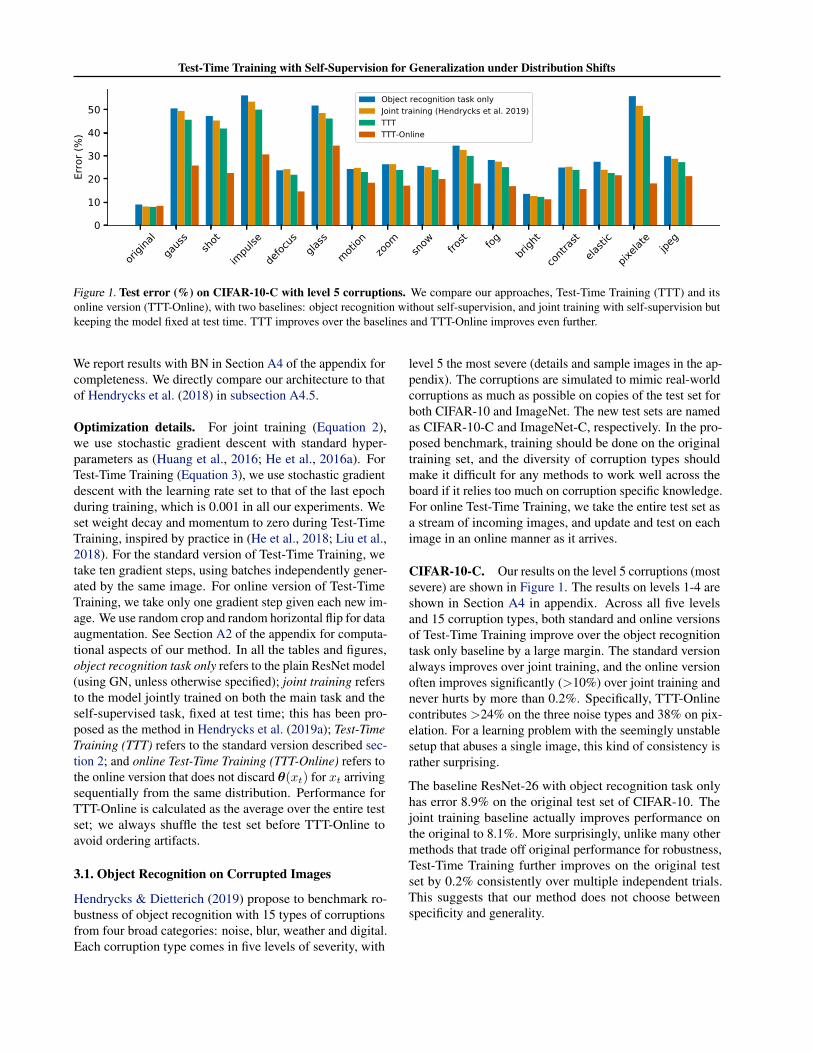
Figure 1. Test error (%) on CIFAR-10-C with level 5 corruptions. We compare our approaches, Test-Time Training (TTT) and itsonline version (TTT-Online), with two baselines: object recognition without self-supervision, and joint training with self-supervision butkeeping the model fixed at test time. TTT improves over the baselines and TTT-Online improves even further.

We report results with BN in Section A4 of the appendix forcompleteness. We directly compare our architecture to thatof Hendrycks et al. (2018) in subsection A4.5.

Optimization details. For joint training (Equation 2),we use stochastic gradient descent with standard hyper-parameters as (Huang et al., 2016; He et al., 2016a). ForTest-Time Training (Equation 3), we use stochastic gradientdescent with the learning rate set to that of the last epochduring training, which is 0.001 in all our experiments. Weset weight decay and momentum to zero during Test-TimeTraining, inspired by practice in (He et al., 2018; Liu et al.,2018). For the standard version of Test-Time Training, wetake ten gradient steps, using batches independently gener-ated by the same image. For online version of Test-TimeTraining, we take only one gradient step given each new im-age. We use random crop and random horizontal flip for dataaugmentation. See Section A2 of the appendix for computa-tional aspects of our method. In all the tables and figures,object recognition task only refers to the plain ResNet model(using GN, unless otherwise specified); joint training refersto the model jointly trained on both the main task and theself-supervised task, fixed at test time; this has been pro-posed as the method in Hendrycks et al. (2019a); Test-TimeTraining (TTT) refers to the standard version described sec-tion 2; and online Test-Time Training (TTT-Online) refers tothe online version that does not discard θ(xt) for xt arrivingsequentially from the same distribution. Performance forTTT-Online is calculated as the average over the entire testset; we always shuffle the test set before TTT-Online toavoid ordering artifacts.

3.1. Object Recognition on Corrupted Images

Hendrycks & Dietterich (2019) propose to benchmark ro-bustness of object recognition with 15 types of corruptionsfrom four broad categories: noise, blur, weather and digital.Each corruption type comes in five levels of severity, with

level 5 the most severe (details and sample images in the ap-pendix). The corruptions are simulated to mimic real-worldcorruptions as much as possible on copies of the test set forboth CIFAR-10 and ImageNet. The new test sets are namedas CIFAR-10-C and ImageNet-C, respectively. In the pro-posed benchmark, training should be done on the originaltraining set, and the diversity of corruption types shouldmake it difficult for any methods to work well across theboard if it relies too much on corruption specific knowledge.For online Test-Time Training, we take the entire test set asa stream of incoming images, and update and test on eachimage in an online manner as it arrives.

CIFAR-10-C. Our results on the level 5 corruptions (mostsevere) are shown in Figure 1. The results on levels 1-4 areshown in Section A4 in appendix. Across all five levelsand 15 corruption types, both standard and online versionsof Test-Time Training improve over the object recognitiontask only baseline by a large margin. The standard versionalways improves over joint training, and the online versionoften improves significantly (>10%) over joint training andnever hurts by more than 0.2%. Specifically, TTT-Onlinecontributes >24% on the three noise types and 38% on pix-elation. For a learning problem with the seemingly unstablesetup that abuses a single image, this kind of consistency israther surprising.

The baseline ResNet-26 with object recognition task onlyhas error 8.9% on the original test set of CIFAR-10. Thejoint training baseline actually improves performance onthe original to 8.1%. More surprisingly, unlike many othermethods that trade off original performance for robustness,Test-Time Training further improves on the original testset by 0.2% consistently over multiple independent trials.This suggests that our method does not choose betweenspecificity and generality.


origin

alga

uss shot

impu

lse

defoc

usgla

ssmoti

onzoo

msno

wfro

st fogbri

ght

contra

stela

stic

pixela

te jpeg

0

20

40

60

Accu

racy

(%)

Object recognition task onlyJoint training (Hendrycks et al. 2019)TTTTTT-Online

0 20000 40000Number of samples

606264666870727476

Accu

racy

(%)

OriginalSliding window average


1215182124273033

Accu

racy

(%)

Gaussian Noise

Sliding window average


161820222426283032

Accu

racy

(%)

Defocus BlurSliding window average


283032343638

Accu

racy

(%)

Zoom Blur



3336394245485154

Accu

racy

(%)

Fog



3033363942454851

Accu

racy

(%)

Elastic Transform


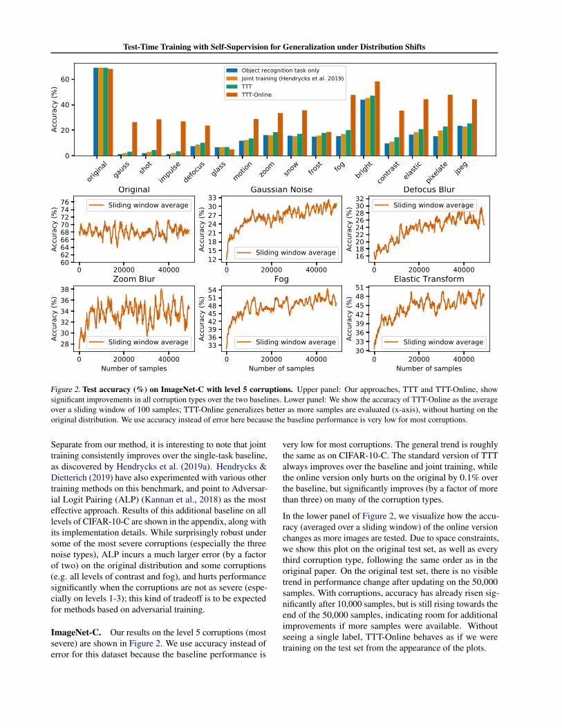
Figure 2. Test accuracy (%) on ImageNet-C with level 5 corruptions. Upper panel: Our approaches, TTT and TTT-Online, showsignificant improvements in all corruption types over the two baselines. Lower panel: We show the accuracy of TTT-Online as the averageover a sliding window of 100 samples; TTT-Online generalizes better as more samples are evaluated (x-axis), without hurting on theoriginal distribution. We use accuracy instead of error here because the baseline performance is very low for most corruptions.

Separate from our method, it is interesting to note that jointtraining consistently improves over the single-task baseline,as discovered by Hendrycks et al. (2019a). Hendrycks &Dietterich (2019) have also experimented with various othertraining methods on this benchmark, and point to Adversar-ial Logit Pairing (ALP) (Kannan et al., 2018) as the mosteffective approach. Results of this additional baseline on alllevels of CIFAR-10-C are shown in the appendix, along withits implementation details. While surprisingly robust undersome of the most severe corruptions (especially the threenoise types), ALP incurs a much larger error (by a factorof two) on the original distribution and some corruptions(e.g. all levels of contrast and fog), and hurts performancesignificantly when the corruptions are not as severe (espe-cially on levels 1-3); this kind of tradeoff is to be expectedfor methods based on adversarial training.

ImageNet-C. Our results on the level 5 corruptions (mostsevere) are shown in Figure 2. We use accuracy instead oferror for this dataset because the baseline performance is

very low for most corruptions. The general trend is roughlythe same as on CIFAR-10-C. The standard version of TTTalways improves over the baseline and joint training, whilethe online version only hurts on the original by 0.1% overthe baseline, but significantly improves (by a factor of morethan three) on many of the corruption types.

In the lower panel of Figure 2, we visualize how the accu-racy (averaged over a sliding window) of the online versionchanges as more images are tested. Due to space constraints,we show this plot on the original test set, as well as everythird corruption type, following the same order as in theoriginal paper. On the original test set, there is no visibletrend in performance change after updating on the 50,000samples. With corruptions, accuracy has already risen sig-nificantly after 10,000 samples, but is still rising towards theend of the 50,000 samples, indicating room for additionalimprovements if more samples were available. Withoutseeing a single label, TTT-Online behaves as if we weretraining on the test set from the appearance of the plots.


orig gauss shot impul defoc glass motn zoom snow frost fog brit contr elast pixel jpeg

TTT-Online 8.2 25.8 22.6 30.6 14.6 34.4 18.3 17.1 20.0 18.0 16.9 11.2 15.6 21.6 18.1 21.2

UDA-SS 9.0 28.2 26.5 20.8 15.6 43.7 24.5 23.8 25.0 24.9 17.2 12.7 11.6 22.1 20.3 22.6

Table 1. Test error (%) on CIFAR-10-C with level 5 corruption. Comparison between online Test-Time Training (TTT-Online) andunsupervised domain adaptation by self-supervision (UDA-SS) (Sun et al., 2019) with access to the entire (unlabeled) test set duringtraining. We highlight the lower error in bold. We have abbreviated the names of the corruptions, in order: original test set, Gaussian noise,shot noise, impulse noise, defocus blur, glass blue, motion blur, zoom blur, snow, frost, fog, brightness, contrast, elastic transformation,pixelation, and JPEG compression. The reported numbers for TTT-Online are the same as in Figure 1. See complete table in Table A2.

0 2000 4000 6000 8000Number of samples

12162024283236404448

Erro

r (%

)

Gaussian NoiseJoint trainingTTTTTT-OnlineUDA-SS


9121518212427303336

Erro

r (%

)

Shot NoiseJoint trainingTTTTTT-OnlineUDA-SS


1520253035404550

Erro

r (%

)

Impulse NoiseJoint trainingTTTTTT-OnlineUDA-SS

Figure 3. Test error (%) on CIFAR-10-C, for the three noise types, with gradually changing distribution. The distribution shifts arecreated by increasing the standard deviation of each noise type from small to large, the further we go on the x-axis. As the samples getnoisier, all methods suffer greater errors the more we evaluate into the test set, but online Test-Time Training (TTT-Online) achieves gentlerslopes than joint training. For the first two noise types, TTT-Online also achieves better results over unsupervised domain adaptation byself-supervision (UDA-SS) (Sun et al., 2019).

Comparison with unsupervised domain adaptation.Table 1 empirically compares online Test-Time Training(TTT-Online) with unsupervised domain adaptation throughself-supervision (UDA-SS) (Sun et al., 2019), which is sim-ilar to our method in spirit but is designed for the setting ofunsupervised domain adaptation (Section 5 provides a sur-vey of other related work in this setting). Given labeled datafrom the training distribution and unlabeled data from thetest distribution, UDA-SS hopes to find an invariant repre-sentation that extracts useful features for both distributionsby learning to perform a self-supervised task, specificallyrotation prediction, simultaneously on data from both. Itthen learns a labeling function on top of the invariant rep-resentation using the labeled data. In our experiments, theunlabeled data given to UDA-SS is the entire test set itselfwithout the labels.

Because TTT-Online can only learn from the unlabeled testsamples that have already been evaluated on, it is given lessinformation than UDA-SS at all times. In this sense, UDA-SS should be regarded as an oracle rather than a baseline.Surprisingly, TTT-Online outperforms UDA-SS on 13 outof the 15 corruptions as well as the original distribution.Our explanation is that UDA-SS has to find an invariantrepresentation for both distributions, while TTT-Online only

adapts the representation to be good for the current testdistribution. That is, TTT-Online has the flexibility to forgetthe training distribution representation, which is no longerrelevant. This suggests that in our setting, forgetting is notharmful and perhaps should even be taken advantage of.

Gradually changing distribution shifts. In our previousexperiments, we have been evaluating the online versionunder the assumption that the test inputs xt for t = 1...n areall sampled from the same test distribution Q, which can bedifferent from the training distribution P . This assumptionis indeed satisfied for i.i.d. samples from a shuffled testset. But here we show that this assumption can in factbe relaxed to allow xt ∼ Qt, where Qt is close to Qt+1

(in the sense of distributional distance). We call this theassumption of gradually changing distribution shifts. Weperform experiments by simulating such distribution shiftson the three noise types of CIFAR-10-C. For each noise type,xt is corrupted with standard deviation σt, and σ1, ..., σninterpolate between the standard deviation of level 1 andlevel 5. So xt is more severely corrupted as we evaluatefurther into the test set and t grows larger. As shown inFigure 3, TTT-Online still improves upon joint training (andour standard version) with this relaxed assumption, and evenupon UDA-SS for the first two noise types.


Accuracy (%) Airplane Bird Car Dog Cat Horse Ship Average

Object recognition task only 67.9 35.8 42.6 14.7 52.0 42.0 66.7 41.4

Joint training (Hendrycks et al., 2019a) 70.2 36.7 42.6 15.5 52.0 44.0 66.7 42.4

TTT (standard version) 70.2 39.2 42.6 21.6 54.7 46.0 77.8 45.2

TTT-Online 70.2 39.2 42.6 22.4 54.7 46.0 77.8 45.4

Table 2. Class-wise and average classification accuracy (%) on CIFAR classes in VID-Robust, adapted from (Shankar et al., 2019).Test-Time Training (TTT) and online Test-Time Training (TTT-Online) improve over the two baselines on average, and by a large marginon “ship” and “dog” classes where the rotation task is more meaningful than in classes like “airplane” (sample images in Figure A7).

3.2. Object Recognition on Video Frames

The Robust ImageNet Video Classification (VID-Robust)dataset was developed by Shankar et al. (2019) from the Ima-geNet Video detection dataset (Russakovsky et al., 2015), todemonstrate how deep models for object recognition trainedon ImageNet (still images) fail to adapt well to video frames.The VID-Robust dataset contains 1109 sets of video framesin 30 classes; each set is a short video clip of frames that aresimilar to an anchor frame. Our results are reported on theanchor frames. To map the 1000 ImageNet classes to the 30VID-Robust classes, we use the max-conversion functionin Shankar et al. (2019). Without any modifications forvideos, we apply our method to VID-Robust on top of thesame ImageNet model as in the previous subsection. Ourclassification accuracy is reported in Table 3.

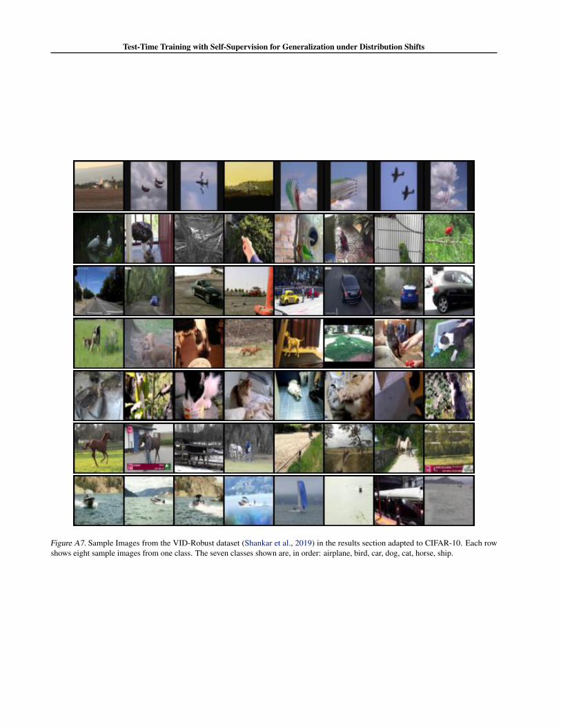
In addition, we take the seven classes in VID-Robust thatoverlap with CIFAR-10, and re-scale those video frames tothe size of CIFAR-10 images, as a new test set for the modeltrained on CIFAR-10 in the previous subsection. Again, weapply our method to this dataset without any modifications.Our results are shown in Table 2, with a breakdown for eachclass. Noticing that Test-Time Training does not improveon the airplane class, we inspect some airplane samples(Figure A7), and observe black margins on two sides of mostimages, which provide a trivial hint for rotation prediction.In addition, given an image of airplanes in the sky, it isoften impossible even for humans to tell if it is rotated. Thisshows that our method requires the self-supervised task tobe both well defined and non-trivial.

3.3. CIFAR-10.1: Unknown Distribution Shifts

CIFAR-10.1 (Recht et al., 2018) is a new test set of size 2000modeled after CIFAR-10, with the exact same classes andimage dimensionality, following the dataset creation processdocumented by the original CIFAR-10 paper as closely aspossible. The purpose is to investigate the distribution shiftspresent between the two test sets, and the effect on objectrecognition. All models tested by the authors suffer a largeperformance drop on CIFAR-10.1 comparing to CIFAR-10,even though there is no human noticeable difference, and

Method Accuracy (%)

Object recognition task only 62.7

Joint training (Hendrycks et al., 2019a) 63.5

TTT (standard version) 63.8

TTT-Online 64.3

Table 3. Test accuracy (%) on VID-Robust dataset (Shankar et al.,2019). TTT and TTT-Online improve over the baselines.

Method Error (%)

Object recognition task only 17.4

Joint training (Hendrycks et al., 2019a) 16.7

TTT (standard version) 15.9

Table 4. Test error (%) on CIFAR-10.1 (Recht et al., 2018). TTT isthe first method to improve the performance of an existing modelon this new test set.

both have the same human accuracy. This demonstrates howinsidious and ubiquitous distribution shifts are, even whenresearchers strive to minimize them.

The distribution shifts from CIFAR-10 to CIFAR-10.1 posean extremely difficult problem, and no prior work has beenable to improve the performance of an existing model onthis new test set, probably because: 1) researchers cannoteven identify the distribution shifts, let alone describe themmathematically; 2) the samples in CIFAR-10.1 are onlyrevealed at test time; and even if they were revealed duringtraining, the distribution shifts are too subtle, and the samplesize is too small, for domain adaptation (Recht et al., 2018).

On the original CIFAR-10 test set, the baseline with onlyobject recognition has error 8.9%, and with joint traininghas 8.1%; comparing to the first two rows of Table 4, bothsuffer the typical performance drop (by a factor of two).TTT yields an improvement of 0.8% (relative improvementof 4.8%) over joint training. We recognize that this improve-ment is small relative to the performance drop, but see it asan encouraging first step for this very difficult problem.


0 10 20 30 40 50 60Gradient inner product

0

1

2

3

4

5Im

prov

emen

t (%

)Level 5Level 4Level 3Level 2Level 1

0 10 20 30 40 50 60Gradient inner product

05

101520253035

Impr

ovem

ent (

%)

Level 5Level 4Level 3Level 2Level 1

Figure 4. Scatter plot of the inner product between the gradients (on the shared feature extractor θe) of the main task lm and the self-supervised task le, and the improvement in test error (%) from Test-Time Training, for the standard (left) and online (right) version. Eachpoint is the average over a test set, and each scatter plot has 75 test sets, from all 15 types of corruptions over five levels as described insubsection 3.1. The blue lines and bands are the best linear fits and the 99% confidence intervals. The linear correlation coefficients are0.93 and 0.89 respectively, indicating strong positive correlation between the two quantities, as suggested by Theorem 1.

4. Theoretical ResultsThis section contains our preliminary study of when and whyTest-Time Training is expected to work. For convex models,we prove that positive gradient correlation between the lossfunctions leads to better performance on the main task afterTest-Time Training. Equipped with this insight, we thenempirically demonstrate that gradient correlation governsthe success of Test-Time Training on the deep learningmodel discussed in Section 3.

Before stating our main theoretical result, we first illustratethe general intuition with a toy model. Consider a regressionproblem where x ∈ Rd denotes the input, y1 ∈ R denotesthe label, and the objective is the square loss (y − y1)2/2for a prediction y. Consider a two layer linear networkparametrized by A ∈ Rh×d and v ∈ Rh (where h standsfor the hidden dimension). The prediction according to thismodel is y = v>Ax, and the main task loss is

lm(x, y1;A,v) =1

2

(y1 − v>Ax

)2. (4)

In addition, consider a self-supervised regression task thatalso uses the square loss and automatically generates a labelys for x. Let the self-supervised head be parametrized byw ∈ Rh. Then the self-supervised task loss is

ls(x, y2;A,w) =1

2

(y2 −w>Ax

)2. (5)

Now we apply Test-Time Training to update the sharedfeature extractor A by one step of gradient descent on ls,which we can compute with y2 known. This gives us

A′ ← A− η(y2 −w>Ax

) (−wx>

), (6)

whereA′ is the updated matrix and η is the learning rate. Ifwe set η = η∗ where

η∗ =y1 − v>Ax

(y2 −w>Ax)v>wx>x, (7)

then with some simple algebra, it is easy to see that themain task loss lm(x, y1;A′,v) = 0. Concretely, Test-TimeTraining drives the main task loss down to zero with a singlegradient step for a carefully chosen learning rate. In prac-tice, this learning rate is unknown since it depends on theunknown y1. However, since our model is convex, as longas η∗ is positive, it suffices to set η to be a small positiveconstant (see details in the appendix). If x 6= 0, one suffi-cient condition for η∗ to be positive (when neither loss iszero) is to have

sign(y1 − v>Ax

)= sign

(y2 −w>Ax

)(8)

and v>w > 0 . (9)

For our toy model, both parts of the condition above have anintuition interpretation. The first part says that the mistakesshould be correlated, in the sense that predictions from bothtasks are mistaken in the same direction. The second part,v>w > 0, says that the decision boundaries on the featurespace should be correlated. In fact, these two parts hold iff.〈∇lm(A),∇ls(A)〉 > 0 (see a simple proof of this fact inthe appendix). To summarize, if the gradients have positivecorrelation, Test-Time Training is guaranteed to reduce themain task loss. Our main theoretical result extends this togeneral smooth and convex loss functions.


Theorem 1. Let lm(x, y;θ) denote the main task loss ontest instance x, y with parameters θ, and ls(x;θ) the self-supervised task loss that only depends on x. Assume that forall x, y, lm(x, y;θ) is differentiable, convex and β-smoothin θ, and both ‖∇lm(x, y;θ)‖ , ‖∇ls(x,θ)‖ ≤ G for all θ.With a fixed learning rate η = ε

βG2 , for every x, y such that

〈∇lm(x, y;θ),∇ls(x;θ)〉 > ε, (10)

we have

lm(x, y;θ) > lm(x, y;θ(x)), (11)

where θ(x) = θ − η∇ls(x;θ) i.e. Test-Time Training withone step of gradient descent.

The proof uses standard techniques in optimization, and isleft for the appendix. Theorem 1 reveals gradient correlationas a determining factor of the success of Test-Time Trainingin the smooth and convex case. In Figure 4, we empiricallyshow that our insight also holds for non-convex loss func-tions, on the deep learning model and across the diverse setof corruptions considered in Section 3; stronger gradient cor-relation clearly indicates more performance improvementover the baseline.

5. Related WorkLearning on test instances. Shocher et al. (2018) pro-vide a key inspiration for our work by showing that imagesuper-resolution could be learned at test time simply by try-ing to upsample a downsampled version of the input image.More recently, Bau et al. (2019) improve photo manipula-tion by adapting a pre-trained GAN to the statistics of theinput image. One of the earlier examples of this idea comesfrom Jain & Learned-Miller (2011), who improve Viola-Jones face detection (Viola et al., 2001) by bootstrappingthe more difficult faces in an image from the more easilydetected faces in that same image. The online version ofour algorithm is inspired by the work of Mullapudi et al.(2018), which makes video segmentation more efficient byusing a student model that learns online from a teachermodel. The idea of online updates has also been used inKalal et al. (2011) for tracking and detection. A recent workin echocardiography (Zhu et al., 2019) improves the deeplearning model that tracks myocardial motion and cardiacblood flow with sequential updates. Lastly, we share thephilosophy of transductive learning (Vapnik, 2013; Gam-merman et al., 1998), but have little in common with theirclassical algorithms; recent work by Tripuraneni & Mackey(2019) theoretically explores this for linear prediction, inthe context of debiasing the LASSO estimator.

Self-supervised learning studies how to create labelsfrom the data, by designing various pretext tasks that can

learn semantic information without human annotations, suchas context prediction (Doersch et al., 2015), solving jig-saw puzzles (Noroozi & Favaro, 2016), colorization (Lars-son et al., 2017; Zhang et al., 2016), noise prediction (Bo-janowski & Joulin, 2017), feature clustering (Caron et al.,2018). Our paper uses rotation prediction (Gidaris et al.,2018). Asano et al. (2019) show that self-supervised learn-ing on only a single image, surprisingly, can produce low-level features that generalize well. Closely related to ourwork, Hendrycks et al. (2019a) propose that jointly traininga main task and a self-supervised task (our joint trainingbaseline in Section 3) can improve robustness on the maintask. The same idea is used in few-shot learning (Su et al.,2019), domain generalization (Carlucci et al., 2019), andunsupervised domain adaptation (Sun et al., 2019).

Adversarial robustness studies the robust riskRP,∆(θ) = Ex,y∼P maxδ∈∆ l(x + δ, y; θ), where lis some loss function, and ∆ is the set of perturbations; ∆is often chosen as the Lp ball, for p ∈ {1, 2,∞}. Manypopular algorithms formulate and solve this as a robustoptimization problem (Goodfellow et al., 2014; Madry et al.,2017; Sinha et al., 2017; Raghunathan et al., 2018; Wong &Kolter, 2017; Croce et al., 2018), and the most well knowntechnique is adversarial training. Another line of workis based on randomized smoothing (Cohen et al., 2019;Salman et al., 2019), while some other approaches, such asinput transformations (Guo et al., 2017; Song et al., 2017),are shown to be less effective (Athalye et al., 2018). Thereare two main problems with the approaches above. First, allof them can be seen as smoothing the decision boundary.This establishes a theoretical tradeoff between accuracy androbustness (Tsipras et al., 2018; Zhang et al., 2019), whichwe also observe empirically with our adversarial trainingbaseline in Section 3. Intuitively, the more diverse ∆ is, theless effective this one-boundary-fits-all approach can be fora particular element of ∆. Second, adversarial methodsrely heavily on the mathematical structure of ∆, whichmight not accurately model perturbations in the real world.Therefore, generalization remains hard outside of the ∆ weknow in advance or can mathematically model, especiallyfor non-adversarial distribution shifts. Empirically, Kanget al. (2019) shows that robustness for one ∆ might nottransfer to another, and training on the L∞ ball actuallyhurts robustness on the L1 ball.

Non-adversarial robustness studies the effect of corrup-tions, perturbations, out-of-distribution examples, and real-world distribution shifts (Hendrycks et al., 2019b;a; 2018;Hendrycks & Gimpel, 2016). Geirhos et al. (2018) showthat training on images corrupted by Gaussian noise makesdeep learning models robust to this particular noise type,but does not improve performance on images corrupted byanother noise type e.g. salt-and-pepper noise.


Unsupervised domain adaptation (a.k.a. transfer learn-ing) studies the problem of distribution shifts, when anunlabeled dataset from the test distribution (target domain)is available at training time, in addition to a labeled datasetfrom the training distribution (source domain) (Chen et al.,2011; Gong et al., 2012; Long et al., 2015; Ganin et al.,2016; Long et al., 2016; Tzeng et al., 2017; Hoffman et al.,2017; Csurka, 2017; Chen et al., 2018). The limitation ofthe problem setting, however, is that generalization mightonly be improved for this specific test distribution, whichcan be difficult to anticipate in advance. Prior work try toanticipate broader distributions by using multiple and evolv-ing domains (Hoffman et al., 2018; 2012; 2014). Test-TimeTraining does not anticipate any test distribution, by chang-ing the setting of unsupervised domain adaptation, whiletaking inspiration from its algorithms. Our paper is a follow-up to Sun et al. (2019), which we explain and empiricallycompare with in Section 3. Our update rule can be viewedas performing one-sample unsupervised domain adaptationon the fly, with the caveat that standard domain adaptationtechniques might become ill-defined when there is only onesample from the target domain.

Domain generalization studies the setting where a metadistribution generates multiple environment distributions,some of which are available during training (source), whileothers are used for testing (target) (Li et al., 2018; Shankaret al., 2018; Muandet et al., 2013; Balaji et al., 2018; Ghifaryet al., 2015; Motiian et al., 2017; Li et al., 2017a; Gan et al.,2016). With only a few environments, information on themeta distribution is often too scarce to be helpful, and withmany environments, we are back to the i.i.d. setting whereeach environment can be seen as a sample, and a strongbaseline is to simply train on all the environments (Li et al.,2019). The setting of domain generalization is limited bythe inherent tradeoff between specificity and generality of afixed decision boundary, and the fact that generalization isagain elusive outside of the meta distribution i.e. the actualP learned by the algorithm.

One (few)-shot learning studies how to learn a new taskor a new classification category using only one (or a few)sample(s), on top of a general representation that has beenlearned on diverse samples (Snell et al., 2017; Vinyals et al.,2016; Fei-Fei et al., 2006; Ravi & Larochelle, 2016; Liet al., 2017b; Finn et al., 2017; Gidaris & Komodakis, 2018).Our update rule can be viewed as performing one-shot self-supervised learning and can potentially be improved byprogress in one-shot learning.

Continual learning (a.k.a. learning without forgetting)studies the setting where a model is made to learn a sequenceof tasks, and not forget about the earlier ones while trainingfor the later (Li & Hoiem, 2017; Lopez-Paz & Ranzato,

2017; Kirkpatrick et al., 2017; Santoro et al., 2016). Incontrast, with Test-Time Training, we are not concernedabout forgetting the past test samples since they have alreadybeen evaluated on; and if a past sample comes up by anychance, it would go through Test-Time Training again. Inaddition, the impact of forgetting the training set is minimal,because both tasks have already been jointly trained.

Online learning (a.k.a. online optimization) is a well-studied area of learning theory (Shalev-Shwartz et al., 2012;Hazan et al., 2016). The basic setting repeats the following:receive xt, predict yt, receive yt from a worst-case oracle,and learn. Final performance is evaluated using the regret,which colloquially translates to how much worse the onlinelearning algorithm performs in comparison to the best fixedmodel in hindsight. In contrast, our setting never revealsany yt during testing even for the online version, so we donot need to invoke the concept of the worst-case oracle orthe regret. Also, due to the lack of feedback from the envi-ronment after predicting, our algorithm is motivated to learn(with self-supervision) before predicting yt instead of after.Note that some of the previously covered papers (Hoffmanet al., 2014; Jain & Learned-Miller, 2011; Mullapudi et al.,2018) use the term “online learning” outside of the learningtheory setting, so the term can be overloaded.

6. DiscussionThe idea of test-time training also makes sense for othertasks, such as segmentation and detection, and in other fields,such as speech recognition and natural language process-ing. For machine learning practitioners with prior domainknowledge in their respective fields, their expertise can beleveraged to design better special-purpose self-supervisedtasks for test-time training. Researchers for general-purposeself-supervised tasks can also use test-time training as anevaluation benchmark, in addition to the currently prevalentbenchmark of pre-training and fine-tuning.

More generally, we hope this paper can encourage re-searchers to abandon the self-imposed constraint of a fixeddecision boundary for testing, or even the artificial divisionbetween training and testing altogether. Our work is buta small step toward a new paradigm where much of thelearning happens after a model is deployed.

Acknowledgements. This work is supported by NSFgrant 1764033, DARPA and Berkeley DeepDrive. Thispaper took a long time to develop, and benefited from con-versations with many of our colleagues, including Ben Rechtand his students Ludwig Schmidt, Vaishaal Shanker andBecca Roelofs; Ravi Teja Mullapudi, Achal Dave and DevaRamanan; and Armin Askari, Allan Jabri, Ashish Kumar,Angjoo Kanazawa and Jitendra Malik.


ReferencesAsano, Y. M., Rupprecht, C., and Vedaldi, A. Surprising

effectiveness of few-image unsupervised feature learning.arXiv preprint arXiv:1904.13132, 2019.

Athalye, A., Carlini, N., and Wagner, D. Obfuscatedgradients give a false sense of security: Circumvent-ing defenses to adversarial examples. arXiv preprintarXiv:1802.00420, 2018.

Balaji, Y., Sankaranarayanan, S., and Chellappa, R. Metareg:Towards domain generalization using meta-regularization.In Advances in Neural Information Processing Systems,pp. 998–1008, 2018.

Bau, D., Strobelt, H., Peebles, W., Wulff, J., Zhou, B., Zhu,J.-Y., and Torralba, A. Semantic photo manipulation witha generative image prior. ACM Transactions on Graphics(TOG), 38(4):59, 2019.

Bojanowski, P. and Joulin, A. Unsupervised learning bypredicting noise. In Proceedings of the 34th InternationalConference on Machine Learning-Volume 70, pp. 517–526. JMLR. org, 2017.

Carlucci, F. M., D’Innocente, A., Bucci, S., Caputo, B., andTommasi, T. Domain generalization by solving jigsawpuzzles. In Proceedings of the IEEE Conference on Com-puter Vision and Pattern Recognition, pp. 2229–2238,2019.

Caron, M., Bojanowski, P., Joulin, A., and Douze, M. Deepclustering for unsupervised learning of visual features. InProceedings of the European Conference on ComputerVision (ECCV), pp. 132–149, 2018.

Caruana, R. Multitask learning. Machine learning, 28(1):41–75, 1997.

Chen, M., Weinberger, K. Q., and Blitzer, J. Co-training fordomain adaptation. In Advances in neural informationprocessing systems, pp. 2456–2464, 2011.

Chen, X., Sun, Y., Athiwaratkun, B., Cardie, C., and Wein-berger, K. Adversarial deep averaging networks for cross-lingual sentiment classification. Transactions of the Asso-ciation for Computational Linguistics, 6:557–570, 2018.

Cohen, J. M., Rosenfeld, E., and Kolter, J. Z. Certifiedadversarial robustness via randomized smoothing. arXivpreprint arXiv:1902.02918, 2019.

Croce, F., Andriushchenko, M., and Hein, M. Provablerobustness of relu networks via maximization of linearregions. arXiv preprint arXiv:1810.07481, 2018.

Csurka, G. Domain adaptation for visual applications: Acomprehensive survey. arXiv preprint arXiv:1702.05374,2017.

Ding, G. W., Wang, L., and Jin, X. AdverTorch v0.1: Anadversarial robustness toolbox based on pytorch. arXivpreprint arXiv:1902.07623, 2019.

Doersch, C., Gupta, A., and Efros, A. A. Unsupervisedvisual representation learning by context prediction. InProceedings of the IEEE International Conference onComputer Vision, pp. 1422–1430, 2015.

Fei-Fei, L., Fergus, R., and Perona, P. One-shot learning ofobject categories. IEEE transactions on pattern analysisand machine intelligence, 28(4):594–611, 2006.

Finn, C., Abbeel, P., and Levine, S. Model-agnostic meta-learning for fast adaptation of deep networks. In Proceed-ings of the 34th International Conference on MachineLearning-Volume 70, pp. 1126–1135. JMLR. org, 2017.

Gammerman, A., Vovk, V., and Vapnik, V. Learning bytransduction. In Proceedings of the Fourteenth conferenceon Uncertainty in artificial intelligence, pp. 148–155.Morgan Kaufmann Publishers Inc., 1998.

Gan, C., Yang, T., and Gong, B. Learning attributes equalsmulti-source domain generalization. In Proceedings ofthe IEEE Conference on Computer Vision and PatternRecognition, pp. 87–97, 2016.

Ganin, Y., Ustinova, E., Ajakan, H., Germain, P., Larochelle,H., Laviolette, F., Marchand, M., and Lempitsky, V.Domain-adversarial training of neural networks. TheJournal of Machine Learning Research, 17(1):2096–2030,2016.

Geirhos, R., Temme, C. R., Rauber, J., Schutt, H. H., Bethge,M., and Wichmann, F. A. Generalisation in humans anddeep neural networks. In Advances in Neural InformationProcessing Systems, pp. 7538–7550, 2018.

Ghifary, M., Bastiaan Kleijn, W., Zhang, M., and Balduzzi,D. Domain generalization for object recognition withmulti-task autoencoders. In Proceedings of the IEEEinternational conference on computer vision, pp. 2551–2559, 2015.

Gidaris, S. and Komodakis, N. Dynamic few-shot visuallearning without forgetting. In Proceedings of the IEEEConference on Computer Vision and Pattern Recognition,pp. 4367–4375, 2018.

Gidaris, S., Singh, P., and Komodakis, N. Unsupervised rep-resentation learning by predicting image rotations. arXivpreprint arXiv:1803.07728, 2018.

Gong, B., Shi, Y., Sha, F., and Grauman, K. Geodesic flowkernel for unsupervised domain adaptation. In 2012 IEEEConference on Computer Vision and Pattern Recognition,pp. 2066–2073. IEEE, 2012.


Goodfellow, I. J., Shlens, J., and Szegedy, C. Explain-ing and harnessing adversarial examples. arXiv preprintarXiv:1412.6572, 2014.

Guo, C., Rana, M., Cisse, M., and van der Maaten, L. Coun-tering adversarial images using input transformations.arXiv preprint arXiv:1711.00117, 2017.

Hazan, E. et al. Introduction to online convex optimization.Foundations and Trends® in Optimization, 2(3-4):157–325, 2016.

He, K., Zhang, X., Ren, S., and Sun, J. Deep residual learn-ing for image recognition. In Proceedings of the IEEEconference on computer vision and pattern recognition,pp. 770–778, 2016a.

He, K., Zhang, X., Ren, S., and Sun, J. Identity mappingsin deep residual networks. In European conference oncomputer vision, pp. 630–645. Springer, 2016b.

He, K., Girshick, R., and Dollar, P. Rethinking imagenetpre-training. arXiv preprint arXiv:1811.08883, 2018.

Hendrycks, D. and Dietterich, T. Benchmarking neuralnetwork robustness to common corruptions and perturba-tions. arXiv preprint arXiv:1903.12261, 2019.

Hendrycks, D. and Gimpel, K. A baseline for detectingmisclassified and out-of-distribution examples in neuralnetworks. arXiv preprint arXiv:1610.02136, 2016.

Hendrycks, D., Mazeika, M., Wilson, D., and Gimpel, K.Using trusted data to train deep networks on labels cor-rupted by severe noise. In Advances in neural informationprocessing systems, pp. 10456–10465, 2018.

Hendrycks, D., Lee, K., and Mazeika, M. Using pre-trainingcan improve model robustness and uncertainty. arXivpreprint arXiv:1901.09960, 2019a.

Hendrycks, D., Mazeika, M., Kadavath, S., and Song, D.Improving model robustness and uncertainty estimateswith self-supervised learning. arXiv preprint, 2019b.

Hoffman, J., Kulis, B., Darrell, T., and Saenko, K. Discover-ing latent domains for multisource domain adaptation. InEuropean Conference on Computer Vision, pp. 702–715.Springer, 2012.

Hoffman, J., Darrell, T., and Saenko, K. Continuous man-ifold based adaptation for evolving visual domains. InProceedings of the IEEE Conference on Computer Visionand Pattern Recognition, pp. 867–874, 2014.

Hoffman, J., Tzeng, E., Park, T., Zhu, J.-Y., Isola, P.,Saenko, K., Efros, A. A., and Darrell, T. Cycada: Cycle-consistent adversarial domain adaptation. arXiv preprintarXiv:1711.03213, 2017.

Hoffman, J., Mohri, M., and Zhang, N. Algorithms andtheory for multiple-source adaptation. In Advances inNeural Information Processing Systems, pp. 8246–8256,2018.

Huang, G., Sun, Y., Liu, Z., Sedra, D., and Weinberger,K. Q. Deep networks with stochastic depth. In Europeanconference on computer vision, pp. 646–661. Springer,2016.

Ioffe, S. and Szegedy, C. Batch normalization: Acceleratingdeep network training by reducing internal covariate shift.arXiv preprint arXiv:1502.03167, 2015.

Jain, V. and Learned-Miller, E. Online domain adaptationof a pre-trained cascade of classifiers. In CVPR 2011, pp.577–584. IEEE, 2011.

Kalal, Z., Mikolajczyk, K., and Matas, J. Tracking-learning-detection. IEEE transactions on pattern analysis andmachine intelligence, 34(7):1409–1422, 2011.

Kang, D., Sun, Y., Brown, T., Hendrycks, D., and Steinhardt,J. Transfer of adversarial robustness between perturbationtypes. arXiv preprint arXiv:1905.01034, 2019.

Kannan, H., Kurakin, A., and Goodfellow, I. Adversariallogit pairing. arXiv preprint arXiv:1803.06373, 2018.

Kirkpatrick, J., Pascanu, R., Rabinowitz, N., Veness, J., Des-jardins, G., Rusu, A. A., Milan, K., Quan, J., Ramalho, T.,Grabska-Barwinska, A., et al. Overcoming catastrophicforgetting in neural networks. Proceedings of the nationalacademy of sciences, 114(13):3521–3526, 2017.

Krizhevsky, A. and Hinton, G. Learning multiple layersof features from tiny images. Technical report, Citeseer,2009.

Larsson, G., Maire, M., and Shakhnarovich, G. Colorizationas a proxy task for visual understanding. In CVPR, 2017.

Li, D., Yang, Y., Song, Y.-Z., and Hospedales, T. M. Deeper,broader and artier domain generalization. In Proceed-ings of the IEEE International Conference on ComputerVision, pp. 5542–5550, 2017a.

Li, D., Zhang, J., Yang, Y., Liu, C., Song, Y.-Z., andHospedales, T. M. Episodic training for domain gen-eralization. arXiv preprint arXiv:1902.00113, 2019.

Li, Y., Tian, X., Gong, M., Liu, Y., Liu, T., Zhang, K.,and Tao, D. Deep domain generalization via conditionalinvariant adversarial networks. In Proceedings of theEuropean Conference on Computer Vision (ECCV), pp.624–639, 2018.


Li, Z. and Hoiem, D. Learning without forgetting. IEEEtransactions on pattern analysis and machine intelligence,40(12):2935–2947, 2017.

Li, Z., Zhou, F., Chen, F., and Li, H. Meta-sgd: Learningto learn quickly for few-shot learning. arXiv preprintarXiv:1707.09835, 2017b.

Liu, Z., Sun, M., Zhou, T., Huang, G., and Darrell, T. Re-thinking the value of network pruning. arXiv preprintarXiv:1810.05270, 2018.

Long, M., Cao, Y., Wang, J., and Jordan, M. I. Learn-ing transferable features with deep adaptation networks.arXiv preprint arXiv:1502.02791, 2015.

Long, M., Zhu, H., Wang, J., and Jordan, M. I. Unsuperviseddomain adaptation with residual transfer networks. InAdvances in Neural Information Processing Systems, pp.136–144, 2016.

Lopez-Paz, D. and Ranzato, M. Gradient episodic memoryfor continual learning. In Advances in Neural InformationProcessing Systems, pp. 6467–6476, 2017.

Madry, A., Makelov, A., Schmidt, L., Tsipras, D., andVladu, A. Towards deep learning models resistant toadversarial attacks. arXiv preprint arXiv:1706.06083,2017.

Motiian, S., Piccirilli, M., Adjeroh, D. A., and Doretto,G. Unified deep supervised domain adaptation and gen-eralization. In Proceedings of the IEEE InternationalConference on Computer Vision, pp. 5715–5725, 2017.

Muandet, K., Balduzzi, D., and Scholkopf, B. Domaingeneralization via invariant feature representation. InInternational Conference on Machine Learning, pp. 10–18, 2013.

Mullapudi, R. T., Chen, S., Zhang, K., Ramanan, D., andFatahalian, K. Online model distillation for efficientvideo inference. arXiv preprint arXiv:1812.02699, 2018.

Noroozi, M. and Favaro, P. Unsupervised learning of visualrepresentations by solving jigsaw puzzles. In EuropeanConference on Computer Vision, pp. 69–84. Springer,2016.

Raghunathan, A., Steinhardt, J., and Liang, P. Certifieddefenses against adversarial examples. arXiv preprintarXiv:1801.09344, 2018.

Ravi, S. and Larochelle, H. Optimization as a model forfew-shot learning. IEEE transactions on pattern analysisand machine intelligence, 2016.

Recht, B., Roelofs, R., Schmidt, L., and Shankar, V. Docifar-10 classifiers generalize to cifar-10? arXiv preprintarXiv:1806.00451, 2018.

Russakovsky, O., Deng, J., Su, H., Krause, J., Satheesh, S.,Ma, S., Huang, Z., Karpathy, A., Khosla, A., Bernstein,M., Berg, A. C., and Fei-Fei, L. ImageNet Large ScaleVisual Recognition Challenge. International Journal ofComputer Vision (IJCV), 115(3):211–252, 2015. doi:10.1007/s11263-015-0816-y.

Salman, H., Yang, G., Li, J., Zhang, P., Zhang, H., Razen-shteyn, I., and Bubeck, S. Provably robust deep learn-ing via adversarially trained smoothed classifiers. arXivpreprint arXiv:1906.04584, 2019.

Santoro, A., Bartunov, S., Botvinick, M., Wierstra, D., andLillicrap, T. Meta-learning with memory-augmented neu-ral networks. In International conference on machinelearning, pp. 1842–1850, 2016.

Shalev-Shwartz, S. et al. Online learning and online con-vex optimization. Foundations and Trends® in MachineLearning, 4(2):107–194, 2012.

Shankar, S., Piratla, V., Chakrabarti, S., Chaudhuri, S.,Jyothi, P., and Sarawagi, S. Generalizing acrossdomains via cross-gradient training. arXiv preprintarXiv:1804.10745, 2018.

Shankar, V., Dave, A., Roelofs, R., Ramanan, D., Recht, B.,and Schmidt, L. Do image classifiers generalize acrosstime? arXiv, 2019.

Shocher, A., Cohen, N., and Irani, M. zero-shot super-resolution using deep internal learning. In Proceedingsof the IEEE Conference on Computer Vision and PatternRecognition, pp. 3118–3126, 2018.

Sinha, A., Namkoong, H., and Duchi, J. Certifying some dis-tributional robustness with principled adversarial training.arXiv preprint arXiv:1710.10571, 2017.

Snell, J., Swersky, K., and Zemel, R. Prototypical networksfor few-shot learning. In Advances in Neural InformationProcessing Systems, pp. 4077–4087, 2017.

Song, Y., Kim, T., Nowozin, S., Ermon, S., and Kushman, N.Pixeldefend: Leveraging generative models to understandand defend against adversarial examples. arXiv preprintarXiv:1710.10766, 2017.

Su, J.-C., Maji, S., and Hariharan, B. Boosting supervi-sion with self-supervision for few-shot learning. arXivpreprint arXiv:1906.07079, 2019.

Sun, Y., Tzeng, E., Darrell, T., and Efros, A. A. Unsuper-vised domain adaptation through self-supervision. arXivpreprint, 2019.


Tripuraneni, N. and Mackey, L. Debiasing linear prediction.arXiv preprint arXiv:1908.02341, 2019.

Tsipras, D., Santurkar, S., Engstrom, L., Turner, A., andMadry, A. Robustness may be at odds with accuracy.arXiv preprint arXiv:1805.12152, 2018.

Tzeng, E., Hoffman, J., Saenko, K., and Darrell, T. Adver-sarial discriminative domain adaptation. In Proceedingsof the IEEE Conference on Computer Vision and PatternRecognition, pp. 7167–7176, 2017.

Vapnik, V. The nature of statistical learning theory. Springerscience & business media, 2013.

Vinyals, O., Blundell, C., Lillicrap, T., Wierstra, D., et al.Matching networks for one shot learning. In Advances inneural information processing systems, pp. 3630–3638,2016.

Viola, P., Jones, M., et al. Rapid object detection using aboosted cascade of simple features. CVPR (1), 1(511-518):3, 2001.

Wong, E. and Kolter, J. Z. Provable defenses against adver-sarial examples via the convex outer adversarial polytope.arXiv preprint arXiv:1711.00851, 2017.

Zhang, H., Yu, Y., Jiao, J., Xing, E. P., Ghaoui, L. E., and Jor-dan, M. I. Theoretically principled trade-off between ro-bustness and accuracy. arXiv preprint arXiv:1901.08573,2019.

Zhang, R., Isola, P., and Efros, A. A. Colorful image col-orization. In European conference on computer vision,pp. 649–666. Springer, 2016.

Zhu, W., Huang, Y., Vannan, M. A., Liu, S., Xu, D., Fan, W.,Qian, Z., and Xie, X. Neural multi-scale self-supervisedregistration for echocardiogram dense tracking. arXivpreprint arXiv:1906.07357, 2019.

Appendix: Test-Time Training with Self-Supervisionfor Generalization under Distribution Shifts

A1. Informal Discussion on Our VariableDecision Boundary

In the introduction, we claim that in traditional supervisedlearning θ gives a fixed decision boundary, while our θ givesa variable decision boundary. Here we informally discussthis claim.

Denote the input space X and output space Y . A decisionboundary is simply a mapping f : X → Y . Let Θ be amodel class e.g Rd. Now consider a family of parametrizedfunctions gθ : X → Y , where θ ∈ Θ. In the context of deeplearning, g is the neural network architecture and θ containsthe parameters. We say that f is a fixed decision boundaryw.r.t. g and Θ if there exists θ ∈ Θ s.t. f(x) = gθ(x)for every x ∈ X , and a variable decision boundary if forevery x ∈ X , there exists θ ∈ Θ s.t. f(x) = gθ(x). Notehow selection of θ can depend on x for a variable decisionboundary, and cannot for a fixed one. It is then trivial toverify that our claim is true under those definitions.

A critical reader might say that with an arbitrarily largemodel class, can’t every decision boundary be fixed? Yes,but this is not the end of the story. Let d = dim(X ) ×dim(Y), and consider the enormous model class Θ′ = Rdwhich is capable of representing all possible mappings be-tween X and Y . Let g′θ′ simply be the mapping representedby θ′ ∈ Θ′. A variable decision boundary w.r.t. g and Θthen indeed must be a fixed decision boundary w.r.t. g′ andΘ′, but we would like to note two things. First, without anyprior knowledge, generalization in Θ′ is impossible withany finite amount of training data; reasoning about g′ andΘ′ is most likely not productive from an algorithmic pointof view, and the concept of a variable decision boundary isto avoid such reasoning. Second, selecting θ based on x fora variable decision boundary can be thought of as “training”on all points x ∈ Rd; however, “training” only happenswhen necessary, for the x that it actually encounters.

Altogether, the concept of a variable decision boundary isdifferent from what can be described by traditional learningtheory. A formal discussion is beyond the scope of thispaper and might be of interest to future work.

A2. Computational Aspects of Our MethodAt test time, our method is 2 × batch size ×number of iterations times slower than regular test-ing, which only performs a single forward pass for eachsample. As the first work on Test-Time Training, thispaper is not as concerned about computational efficiencyas improving robustness, but here we provide two poten-tial solutions that might be useful, but have not been thor-oughly verified. The first is to use the thresholding trickon ls, introduced as a solution for the small batches prob-lem in the method section. For the models considered inour experiments, roughly 80% of the test instances fallbelow the threshold, so Test-Time Training can only beperformed on the other 20% without much effect on per-formance, because those 20% contain most of the sam-ples with wrong predictions. The second is to reducethe number of iterations of test-time updates. Forthe online version, the number of iterations is al-ready 1, so there is nothing to do. For the standard ver-sion, we have done some preliminary experiments settingnumber of iterations to 1 (instead of 10) and learn-ing rate to 0.01 (instead of 0.001), and observing resultsalmost as good as the standard hyper-parameter setting. Amore in depth discussion on efficiency is left for futureworks, which might, during training, explicitly make themodel amenable to fast updates.

A3. ProofsHere we prove the theoretical results in the main paper.

A3.1. The Toy Problem

The following setting applies to the two lemmas; this issimply the setting of our toy problem, reproduced here forease of reference.


Consider a two layer linear network parametrized byA ∈Rh×d (shared) and v,w ∈ Rh (fixed) for the two heads,respectively. Denote x ∈ Rd the input and y1, y2 ∈ R thelabels for the two tasks, respectively. For the main task loss

lm(A;v) =1

2

(y1 − v>Ax

)2, (12)

and the self-supervised task loss

ls(A;w) =1

2

(y2 −w>Ax

)2, (13)

Test-Time Training yields an updated matrix

A′ ← A− η(y2 −w>Ax

) (−wx>

), (14)

where η is the learning rate.Lemma 1. Following the exposition of the main paper, let

η∗ =(y1 − v>Ax)

(y2 − w>Ax)v>wx>x. (15)

Assume η∗ ∈ [ε,∞) for some ε > 0. Then for any η ∈ (0, ε],we are guaranteed an improvement on the main loss i.e.lm(A′) < lm(A).

Proof. From the exposition of the main paper, we know that

lm(A− η∗∇lsA)) = 0,

which can also be derived from simple algebra. Then byconvexity, we have

lm (A− η∇ls(A)) (16)

= lm

((1− η

η∗

)A+

η

η∗(A− η∗∇ls(A))

)(17)

≤(

1− η

η∗

)lm(A) + 0 (18)

≤(

1− η

ε

)lm(A) (19)

< lm(A), (20)

where the last inequality uses the assumption that lm(A) >0, which holds because η∗ > 0.Lemma 2. Define 〈U ,V 〉 = vec (U)

> vec (V ) i.e. theFrobenious inner product, then

sign (η∗) = sign (〈∇lm(A),∇ls(A)〉) . (21)

Proof. By simple algebra,

〈∇lm(A),∇ls(A)〉= 〈(y1 − v>Ax

) (−vx>

),(y2 −w>Ax

) (−wx>

)〉

=(y1 − v>Ax

) (y2 −w>Ax

)Tr(xv>wx>

)=(y1 − v>Ax

) (y2 −w>Ax

)v>wx>x,

which has the same sign as η∗.

A3.2. Proof of Theorem 1

For any η, by smoothness and convexity,

lm(x, y;θ(x)) = lm(x, y;θ − η∇ls(x;θ))

≤ lm(x, y;θ) + η〈∇lm(x, y;θ),∇ls(x,θ)〉

+η2β

2‖∇ls(x;θ)‖2 .

Denote

η∗ =〈∇lm(x, y;θ),∇ls(x,θ)〉

β ‖∇ls(x;θ)‖2.

Then Equation 22 becomes

lm(x, y;θ − η∗∇ls(x;θ)) (22)

≤ lm(x, y;θ)− 〈∇lm(x, y;θ),∇ls(x,θ)〉2

2β ‖∇ls(x;θ)‖2. (23)

And by our assumptions on the gradient norm and gradientinner product,

lm(x, y;θ)− lm(x, y;θ − η∗∇ls(x;θ)) ≥ ε2

2βG2. (24)

Because we cannot observe η∗ in practice, we instead usea fixed learning rate η = ε

βG2 , as stated in Theorem 1.Now we argue that this fixed learning rate still improvesperformance on the main task.

By our assumptions, η∗ ≥ εβG2 , so η ∈ (0, η∗]. Denote

g = ∇ls(x;θ), then by convexity of lm,

lm(x, y;θ(x)) = lm(x, y;θ − ηg) (25)

= lm

(x, y;

(1− η

η∗

)θ +

η

η∗(θ − η∗g)

)(26)

≤(

1− η

η∗

)lm(x, y;θ) +

η

η∗lm(x, y;θ − η∗g) (27)

Combining with Equation 24, we have

lm(x, y;θ(x)) ≤(

1− η

η∗

)lm(x, y;θ)

+η

η∗

(lm(x, y;θ)− ε2

2βG2

)= lm(x, y;θ)− η

η∗ε2

2βG2

Since η/η∗ > 0, we have shown that

lm(x, y;θ)− lm(x, y;θ(x)) > 0. (28)


A4. Additional Results on the CommonCorruptions Dataset

For table aethetics, we use the following abbreviations: Bfor baseline, JT for joint training, TTT for Test-Time Train-ing standard version, and TTT-Online for online Test-TimeTraining i.e. the online version.

We have abbreviated the names of the corruptions, in order:original test set, Gaussian noise, shot noise, impulse noise,defocus blur, glass blue, motion blur, zoom blur, snow, frost,fog, brightness, contrast, elastic transformation, pixelation,and JPEG compression.

A4.1. Results Using Batch Normalization

As discussed in the results section, Batch Normalization(BN) is ineffective for small batches, which are the inputsfor Test-Time Training (both standard and online version)since there is only one sample available when forming eachbatch; therefore, our main results are based on a ResNetusing Group Normalization (GN). Figure A2 and Table A1show results of our method on CIFAR-10-C level 5, with aResNet using Batch Normalization (BN). These results areonly meant to be a point of reference for the curious readers.

In the early stage of this project, we have experimentedwith two potential solutions to the small batches problemwith BN. The naive solution is to fix the BN layers duringTest-Time Training. but this diminishes the performancegains since there are fewer shared parameters. The bettersolution, adopted for the results below, is hard examplemining: instead of updating on all inputs, we only updateon inputs that incur large self-supervised task loss ls, wherethe large improvements might counter the negative effectsof inaccurate statistics.

Test-Time Training (standard version) is still very effectivewith BN. In fact, some of the improvements are quite dra-matic, such as on contrast (34%), defocus blue (18%) andGaussian noise (22% comparing to joint-training, and 16%comparing to the baseline). Performance on the originaldistribution is still almost the same, and the original errorwith BN is in fact slightly lower than with GN, and takeshalf as many epochs to converge.

We did not further experiment with BN because of two rea-sons: 1) The online version does not work with BN, becausethe problem with inaccurate batch statistics is exacerbatedwhen training online for many (e.g. 10000) steps. 2) Thebaseline error for almost every corruption type is signifi-cantly higher with BN than with GN. Although unrelatedto the main idea of our paper, we make the interesting notethat GN significantly improves model robustness.

A4.2. Additional Baseline: Adversarial Logit Pairing

As discussed in the results section, Hendrycks & Dietterich(2019) point to Adversarial Logit Pairing (ALP) (Kannanet al., 2018) as an effective method for improving modelrobustness to corruptions and perturbations, even thoughit was designed to defend against adversarial attacks. Wetake ALP as an additional baseline on all benchmarks basedon CIFAR-10 (using GN), following the training proce-dure in Kannan et al. (2018) and their recommended hyper-parameters. The implementation of the adversarial attackcomes from the codebase of Ding et al. (2019). We did notrun ALP on ImageNet because the two papers we referencefor this method, Kannan et al. (2018) and Hendrycks & Di-etterich (2019), did not run on ImageNet or make any claimor recommendation.

A4.3. Results on CIFAR-10-C and ImageNet-C, Level 5

Table A2 and Table A3 correspond to the bar plots in theresults section. Two rows of Table A2 have been presentedas Table 1 in the main text.

A4.4. Results on CIFAR-10-C, Levels 1-4

The following bar plots and tables are on levels 1-4 ofCIFAR-10-C. The original distribution is the same for alllevels, so are our results on the original distribution.

A4.5. Direct Comparison with Hendrycks et al. (2019a)

The following comparison has been requested by an anony-mous reviewer for our final version. Our joint trainingbaseline is based on Hendrycks et al. (2019a), but also incor-porates some architectural changes (see below). We foundthese changes improved the robustness of our method, andfelt that it was important to give the baseline the same ben-efit. Note that our joint training baseline overall performsbetter than Hendrycks: Compare Table S2 to Figure 3 ofHendrycks et al. (2019a) (provided by the authors), ourbaseline has average error of 22.8% across all corruptionsand levels, while their average error is 28.6%.

Summary of architectural changes: 1) Group Normalization(GN) instead of Batch Normalization (BN). For complete-ness, the results with BN are provided in Table S1; c.f. GNresults in Table S2 which significantly improves robustness,with or without self-supervision. 2) We split after the sec-ond residual group, while they split after the third residualgroup right before the linear layer. This consistently givesabout 0.5% - 1% improvement. 3) We use a ResNet-26,while they use a 40-2 Wide ResNet. But our baseline stillperforms better than their method even though our networkis 4x smaller, due to the two tricks above.


Gaussian Noise Shot Noise Impulse Noise Defocus Blur Frosted Glass Blur

Motion Blur Zoom Blur Snow Frost Fog

Brightness Contrast Elastic Pixelate JPEG

Figure A1. Sample images from the Common Corruptions Benchmark, taken from the original paper by Hendrycks & Dietterich (2019).

origin

alga

uss shot

impu

lse

defoc

usgla

ssmoti

onzoo

msno

wfro

st fogbri

ght

contra

stela

stic

pixela

te jpeg

0

20

40

60

Erro

r (%

)

Object recognition task onlyJoint training (Hendrycks et al. 2019)TTT

Figure A2. Test error (%) on CIFAR-10-C, level 5, ResNet-26 with Batch Normalization.

orig gauss shot impul defoc glass motn zoom snow frost fog brit contr elast pixel jpegB 7.9 63.9 58.8 64.3 46.3 54.6 41.6 45.9 31.9 44.0 37.5 13.0 69.2 33.8 61.4 31.7JT 7.5 70.7 65.6 67.2 43.1 55.4 40.9 42.7 30.3 44.5 42.5 12.7 58.6 30.7 62.6 31.9

TTT 7.9 47.9 45.2 54.8 27.6 50.4 31.5 30.9 28.7 34.3 26.9 12.6 35.2 30.6 51.2 31.3

Table A1. Test error (%) on CIFAR-10-C, level 5, ResNet-26 with Batch Normalization.


TTT 7.9 45.6 41.8 50.0 21.8 46.1 23.0 23.9 23.9 30.0 25.1 12.2 23.9 22.6 47.2 27.2TTT-Online 8.2 25.8 22.6 30.6 14.6 34.4 18.3 17.1 20.0 18.0 16.9 11.2 15.6 21.6 18.1 21.2

UDA-SS 9.0 28.2 26.5 20.8 15.6 43.7 24.5 23.8 25.0 24.9 17.2 12.7 11.6 22.1 20.3 22.6ALP 16.5 22.7 22.9 28.3 25.0 25.6 27.4 23.1 25.2 27.2 64.8 21.7 73.6 23.0 20.2 18.9

Table A2. Test error (%) on CIFAR-10-C, level 5, ResNet-26.


TTT 69.0 3.1 4.5 3.5 10.1 6.8 13.5 18.5 17.1 17.9 20.0 47.0 14.4 20.9 22.8 25.3TTT-Online 68.8 26.3 28.6 26.9 23.7 6.6 28.7 33.4 35.6 18.7 47.6 58.3 35.3 44.3 47.8 44.3

Table A3. Test accuracy (%) on ImageNet-C, level 5, ResNet-18.


origin

alga

uss shot

impu

lse

defoc

usgla

ssmoti

onzoo

msno

wfro

st fogbri

ght

contra

stela

stic

pixela

te jpeg

0

10

20

30

40

50

Erro

r (%

)


Figure A3. Test error (%) on CIFAR-10-C, level 4. See the results section for details.


TTT 7.9 41.5 35.4 39.8 15.0 47.8 19.1 18.4 20.1 24.0 13.5 10.0 14.1 17.7 29.4 24.5TTT-Online 8.2 22.9 20.0 23.9 11.2 35.1 15.6 13.8 18.6 15.9 12.3 9.7 11.9 16.7 13.6 19.8

ALP 16.5 21.3 20.5 24.5 20.7 25.9 23.7 21.4 24.2 23.9 42.2 17.5 53.7 22.1 19.1 18.5


origin

alga

uss shot

impu

lse

defoc

usgla

ssmoti

onzoo

msno

wfro

st fogbri

ght

contra

stela

stic

pixela

te jpeg

0

10

20

30

40

Erro

r (%

)




TTT 7.9 37.2 31.6 28.6 11.5 35.8 19.1 15.8 17.8 23.3 11.0 9.1 11.6 14.3 18.9 22.3TTT-Online 8.2 21.3 17.7 17.9 9.0 23.4 15.3 12.5 16.4 15.8 10.9 9.0 10.7 12.8 12.2 18.7

ALP 16.5 20.0 19.3 20.5 19.2 21.2 24.0 20.5 20.9 24.2 30.1 16.6 39.6 20.9 17.8 18.0



origin

alga

uss shot

impu

lse

defoc

usgla

ssmoti

onzoo

msno

wfro

st fogbri

ght

contra

stela

stic

pixela

te jpeg

0

10

20

30

40

Erro

r (%

)




TTT 7.9 28.8 20.7 23.0 9.0 36.6 15.4 13.1 20.2 16.9 9.2 8.3 10.2 12.5 14.8 19.7TTT-Online 8.2 16.8 13.8 15.5 8.5 23.4 13.3 11.5 16.8 12.7 9.4 8.4 9.7 12.4 11.5 17.0

ALP 16.5 18.0 17.2 19.0 17.8 20.7 21.2 19.3 19.0 20.1 22.4 16.3 29.2 20.3 17.4 17.8


origin

alga

uss shot

impu

lse

defoc

usgla

ssmoti

onzoo

msno

wfro

st fogbri

ght

contra

stela

stic

pixela

te jpeg

0

10

20

30

40

Erro

r (%

)




TTT 7.9 19.1 15.8 16.5 8.0 37.9 11.7 12.2 12.8 11.9 8.2 8.0 8.3 12.6 11.1 15.5TTT-Online 8.2 13.8 11.9 12.2 8.5 24.4 10.5 11.5 12.4 10.7 8.5 8.3 8.6 12.4 10.7 14.4

ALP 17.0 16.8 17.6 16.8 20.9 18.7 19.0 17.3 17.5 17.4 16.1 18.4 20.4 17.0 17.2 17.5



Figure A7. Sample Images from the VID-Robust dataset (Shankar et al., 2019) in the results section adapted to CIFAR-10. Each rowshows eight sample images from one class. The seven classes shown are, in order: airplane, bird, car, dog, cat, horse, ship.

Date post:	16-Oct-2021
Category:	Documents
Upload:	others
View:	1 times
Download:	0 times

Test-Time Training with Self-Supervision for ...

Documents