ST. ANTHONY FALLS LABORATORY Engineering, Environmental and Geophysical Fluid Dynamics

PROJECT REPORT 467

Testing an Underdrain System under Backwash Flow Conditions for the Chaparral

Water Treatment Plant

By

Chris Ellis, Richard Christopher and Omid Mohseni

Prepared for Johnsons Screens

March 2005 Minneapolis, Minnesota

i

The University of Minnesota is committed to the policy that all persons shall have equal access to its programs, facilities, and employment without regard to race, religion, color, sex, national origin, handicap, age or veteran status.

ii

Abstract

Johnsons Screens was required to test its underdrain system under backwash flow conditions to

assess the uniformity of flow discharge throughout the manifold system. To test the system, a

basin was built in St. Anthony Falls Laboratory and the underdrain system components were

provided and installed by Johnsons Screens. To assess the uniformity of flow of the manifold

system, a measurement technique was developed to determine the flow at a number of locations

at design flows. The technique was a flow-capturing apparatus with an open-topped tank, two

tubes, a hose and a pump. Using this apparatus, the flow was captured over a period of time and

weighed to determine the flow rate from each triplet of orifices. The system error under high

system flow rate (about 19 cfs) was less than 0.7%.

Six locations were determined by Johnsons Screens for the testing. At each location, a total of

five measurements were taken and averaged under the high system flow rate (about 19 cfs) and

an additional five measurements for the low system flow rate (about 4.4 cfs). The results of the

measurements showed that the deviation of the flow measurements from the mean were within

±5% under high system flows and ±7% under low system flows.

iii

Acknowledgements

The work reported herein was funded by Johnsons Screens, and Mr. Thomas Steinke from

Johnsons Screen was the project officer. We would like to thank Mike Plante, Ben Erickson,

Luke Carlson and Matthew Leuker of St. Anthony Falls Laboratory for their contribution to the

model construction, video documentation and data collection.

iv

Table of Contents

Abstract ...........................................................................................................................................ii

Acknowledgements ....................................................................................................................... iii

List of Figures .................................................................................................................................v

List of Tables..................................................................................................................................vi

1. Introduction .................................................................................................................................1

2. Full Scale Facility Set-up ............................................................................................................2

2.1. Weir Calibration...................................................................................................................3

3. Instrumentation............................................................................................................................5

4. Test Results .................................................................................................................................8

4.1. Initial Tests ...........................................................................................................................8

4.2. Final Tests ............................................................................................................................9

5. Summary ...................................................................................................................................15

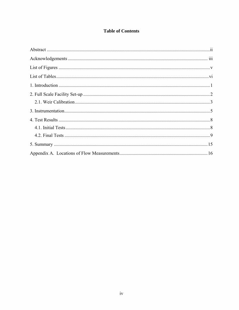
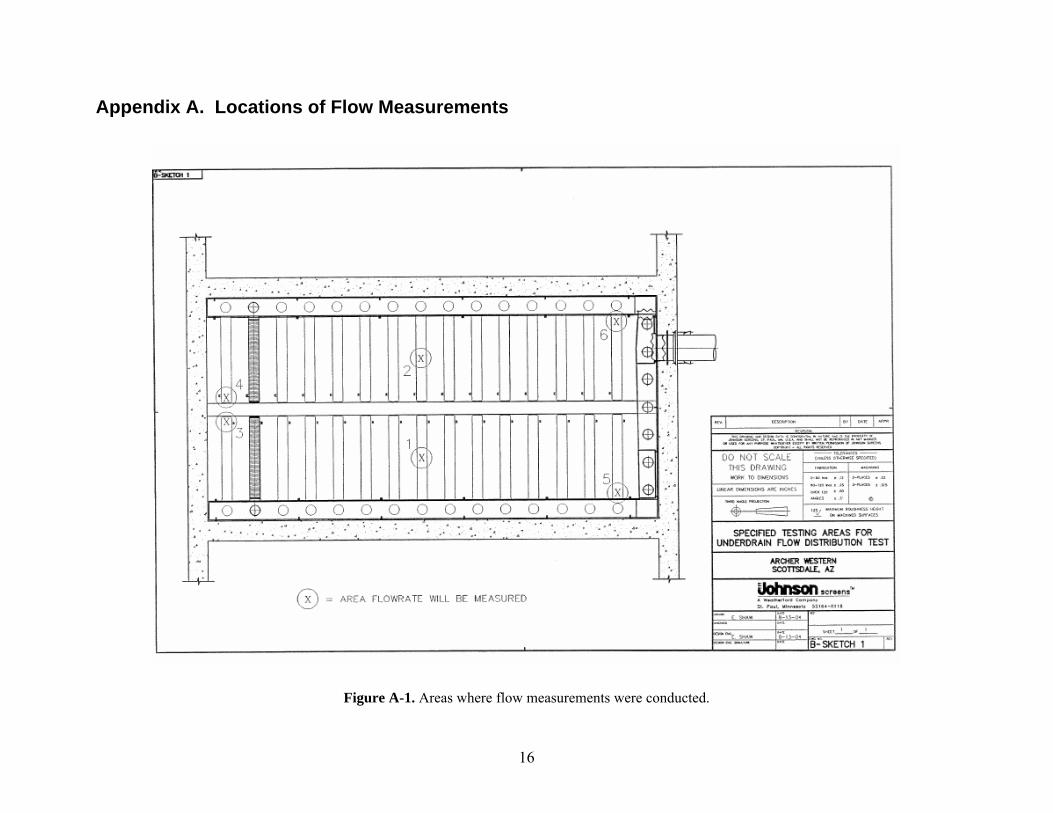
Appendix A. Locations of Flow Measurements...........................................................................16

v

List of Figures

Figure 1. Plan view of the underdrain system. ...............................................................................1 Figure 2. The basin cross-section provided by Johnsons Screens..................................................2 Figure 3. The basin with Johnson Screens underdrain system installed. .......................................3 Figure 4. Schematic of the sharp-crested weir at the downstream end of the basin and the

location of the pressure tap for measuring the static head upstream of the weir. .......4 Figure 5. The discharge-head relationship of the sharp-crested weir.............................................4 Figure 6. The positions of the orifices along and across the laterals..............................................5 Figure 7. The flow capturing tank which was used to measure the flow rate through each row of

orifices.........................................................................................................................7 Figure 8. The test set-up for measuring flow rate ..........................................................................7 Figure 9. Average discharge measurements under high system flows.........................................13 Figure 10. Average discharge measurements under low system flows........................................13 Figure 11. Deviation from the mean of discharge measurements under high system flows........14 Figure 12. Deviation from the mean of discharge measurements under low system flows .........14 Figure A-1. Areas where flow measurements were conducted. ...................................................16

vi

List of Tables

Table 1. Flow measurement data collected under high system flow conditions ..........................10 Table 2. Flow measurement data collected under low system flow conditions ...........................11 Table 3. Test results on 11/22/2004..............................................................................................12

1

1. Introduction

Johnsons Screens was required to test its underdrain system, to be built for the City of Scottsdale,

AZ, under backwash flow conditions to assess the uniformity of flow discharge throughout the

manifold system. Uniform flow distribution is required for efficient and effective operation and

backwash. It was expected that localized excess flow under any specified flow condition would

not exceed ±5 of average flow per square foot of filter area. The system was to be tested under

two different flow conditions, the maximum flow being 8700 gpm (19.4 cfs).

The underdrain system consists of a front manifold, two prismatic headers running down on each

side of the basin, and thirty (30) 8-inch laterals (Figure 1). The headers cross-sectional areas

vary along their lengths. During backwash, water enters the system through a 24-inch pipe, and

is distributed between the two headers through a manifold header pipe.

The scope of this study was to build a basin with the same geometry as the underdrain system

basin, to develop a flow velocity measurement technique with about 2% accuracy, and then to

conduct full scale testing of the Johnsons Screens underdrain system. Testing would consist of

operating the system at the design flows and measuring local discharge of the manifold system at

a number of locations to assess discharge uniformity throughout the system.

Figure 1. Plan view of the underdrain system.

2

2. Full Scale Facility Set-up

The facility included a basin, a sharp-crested weir at the downstream end of the basin, and the

plumbing required to supply approximately 19 cfs. The basin was rectangular (17΄×34΄) with a

6.25% sloped floor built into the basin from the headers towards the middle of the basin, creating

a 6-inch elevation difference between the wall base and the middle of the basin (Figure 2). The

basin walls were 36 inches high, providing a total water depth of 39 inches in the middle of the

basin and 3 inches of free board. The basin was constructed from lumber and plywood and was

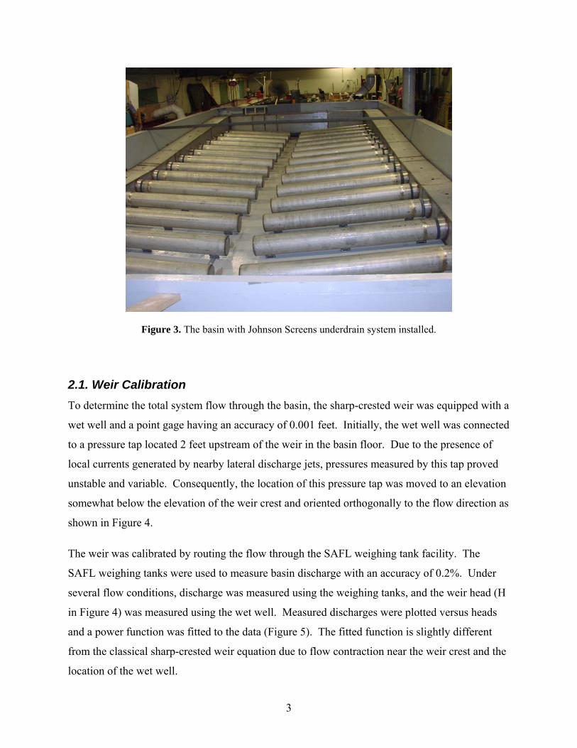
painted and sealed. All components of the underdrain system were provided and installed by

Johnsons Screens (Figure 3). All plumbing outside of the basin, including the 24-inch inlet pipe

and the drain system downstream of the weir, were done by SAFL and was designed to provide

about 19 cfs flow through the system under backwash conditions.

Figure 2. The basin cross-section provided by Johnsons Screens.

A sharp crested weir, with a maximum height of 36 inches was installed at the downstream end

of the basin for system flow measurement. The flow was controlled using valves upstream of the

inlet pipe.

3

Figure 3. The basin with Johnson Screens underdrain system installed.

2.1. Weir Calibration To determine the total system flow through the basin, the sharp-crested weir was equipped with a

wet well and a point gage having an accuracy of 0.001 feet. Initially, the wet well was connected

to a pressure tap located 2 feet upstream of the weir in the basin floor. Due to the presence of

local currents generated by nearby lateral discharge jets, pressures measured by this tap proved

unstable and variable. Consequently, the location of this pressure tap was moved to an elevation

somewhat below the elevation of the weir crest and oriented orthogonally to the flow direction as

shown in Figure 4.

The weir was calibrated by routing the flow through the SAFL weighing tank facility. The

SAFL weighing tanks were used to measure basin discharge with an accuracy of 0.2%. Under

several flow conditions, discharge was measured using the weighing tanks, and the weir head (H

in Figure 4) was measured using the wet well. Measured discharges were plotted versus heads

and a power function was fitted to the data (Figure 5). The fitted function is slightly different

from the classical sharp-crested weir equation due to flow contraction near the weir crest and the

location of the wet well.

4

Figure 4. Schematic of the sharp-crested weir at the downstream end of the basin and the location of the pressure tap for measuring the static head upstream of the weir.

Figure 5. The discharge-head relationship of the sharp-crested weir

y = 58.487x1.3917

R2 = 0.9999

0

2

4

6

8

10

12

14

16

18

20

0 0.1 0.2 0.3 0.4H (ft)

Flow

Ove

r the

Wei

r (cf

s)

5

3. Instrumentation

The purpose of the test program was to assess the uniformity of the manifold system discharge.

To do this, a measurement technique was needed that could determine local manifold discharge

at a number of locations at design flows. There are 28 triplets of orifices on each lateral. At

each triplet location, i.e. cross-section, one orifice was located on the bottom of the pipe and the

other two were offset 45o to either side (Figure 6). Two methods were proposed to measure the

flow rate: (1) using a Sontek Acoustic Doppler Velocimeter (ADV) to measure the velocity of

the jet leaving each orifice, and (2) capturing the flow out of each triplet of orifices and weighing

it over a period of time to arrive at flowrate.

Due to logistics of making precise velocity measurements outside of the orifices, the possible use

of this method was abandoned in favor of the discharge capture concept. The flow-capturing

apparatus was comprised of an open-topped tank, two ¼” tubes, and a 1” flexible hose. The tank

was made of Plexiglas with a width and length of 2.56"and 23", respectively, and could be split

along the vertical centerline to allow repositioning along any lateral in the system.

Figure 6. The positions of the orifices along and across the laterals.

6

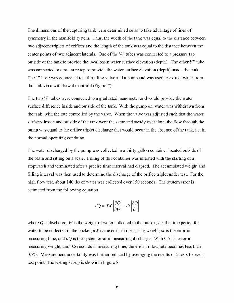
The dimensions of the capturing tank were determined so as to take advantage of lines of

symmetry in the manifold system. Thus, the width of the tank was equal to the distance between

two adjacent triplets of orifices and the length of the tank was equal to the distance between the

center points of two adjacent laterals. One of the ¼” tubes was connected to a pressure tap

outside of the tank to provide the local basin water surface elevation (depth). The other ¼” tube

was connected to a pressure tap to provide the water surface elevation (depth) inside the tank.

The 1” hose was connected to a throttling valve and a pump and was used to extract water from

the tank via a withdrawal manifold (Figure 7).

The two ¼” tubes were connected to a graduated manometer and would provide the water

surface difference inside and outside of the tank. With the pump on, water was withdrawn from

the tank, with the rate controlled by the valve. When the valve was adjusted such that the water

surfaces inside and outside of the tank were the same and steady over time, the flow through the

pump was equal to the orifice triplet discharge that would occur in the absence of the tank, i.e. in

the normal operating condition.

The water discharged by the pump was collected in a thirty gallon container located outside of

the basin and sitting on a scale. Filling of this container was initiated with the starting of a

stopwatch and terminated after a precise time interval had elapsed. The accumulated weight and

filling interval was then used to determine the discharge of the orifice triplet under test. For the

high flow test, about 140 lbs of water was collected over 150 seconds. The system error is

estimated from the following equation

tQdt

WQdWdQ

∂∂

+∂∂

=

where Q is discharge, W is the weight of water collected in the bucket, t is the time period for

water to be collected in the bucket, dW is the error in measuring weight, dt is the error in

measuring time, and dQ is the system error in measuring discharge. With 0.5 lbs error in

measuring weight, and 0.5 seconds in measuring time, the error in flow rate becomes less than

0.7%. Measurement uncertainty was further reduced by averaging the results of 5 tests for each

test point. The testing set-up is shown in Figure 8.

7

Figure 7. The flow capturing tank which was used to measure the flow rate through each row of orifices.

Figure 8. The test set-up for measuring flow rate

8

4. Test Results

The tests were initially done in autumn during an exceptionally long falling leaves season in

Minneapolis. Since all tests were done using essentially unscreened Mississippi River water, a

significant problem was caused by organic debris plugging the orifices and impacting the test

results. Therefore, testing was postponed until the debris in the Mississippi River water

decreased significantly.

4.1. Initial Tests Per the request of Johnsons Screens, six locations were used to conduct flow measurement

testing. The locations are shown in Appendix A (Figure A.1). At each location flow

measurements were conducted for two system flow rates: 18.4 cfs and 4.4 cfs. Each

measurement was repeated 5 times and the results averaged to reduce measurement uncertainty.

Tables 1 and 2 give the results for high and low flow conditions. In addition to the original 60

tests, several tests were repeated to verify the repeatability of the test set-up. Therefore, five

more tests were conducted under high flow conditions at point 1 (TP1), designated by TP1-2 in

Table 1, and five more tests were conducted under low flow conditions at point 2 (TP2),

designated by TP2-2 in Table 2.

Since the system flow varied somewhat from one test to another, a column was added to the

tables to display the orifice triplet discharge adjusted for the system flow for that run in

comparison to mean system flow. The adjusted flow was calculated as follows

s

sm Q

QQQ =

Where Q is the adjusted flow, Qm is the measured flow, Qs is the system flow for that test, and

sQ is the average system flow.

Under high flow conditions, the standard deviation of each set of data collected at a point, i.e. of

five tests at one test point, is less than 0.3% of the average of the set. In the last row of each set

of tests for a given location, the average flow measured for that set was compared with the

average flow of all tests. Under high flow conditions in the system, all measured flows are

9

within ±5% of the average flow. The maximum deviation is 4.8%.

Under low flow conditions, the standard deviation of each set of data collected at a point is less

than 1.5% of the average of the set. In addition, all measured flows are within ±7.1% of the

average flow. This indicates that under low flow conditions there is more variability in the

system.

Table 1 also gives the pressure difference in inches of water between the downstream point of

the 24-inch inlet pipe and the basin. The average pressure differential was recorded to be 24.77

inches of water.

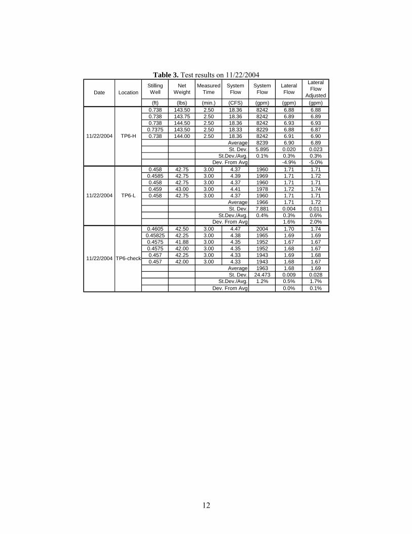
4.2. Final Tests On October 27, 2005, a series of tests were conducted for TP6 in the presence of the Johnsons

Screens representatives. After thorough inspection of the system, it became clear that flow was

less than previous measurements due to clogging of one of the orifices at point TP6. The tests

were repeated on November 22 under both high and low flow conditions. The test results are

summarized in Table 3. The standard deviation of each set of data collected at TP6 is less than

0.5% of the average of the set. All measured flows were less than ±5% of the average flow.

Figures 9 and 10 show the magnitude of flow measurements under high and low system flows,

respectively. Figures 11 and 12 show the deviation from the mean of the flow measurements

under high and low system flows, respectively.

The test results show that under high system flow conditions, flow through orifices varies less

than ±5% when the underdrain system is in backwash mode. Under low system flow conditions,

flow through orifices varies less than ±7%.

10

Table 1. Flow measurement data collected under high system flow conditions

(oF) (in H2O) (ft) (lbs) (min.) (CFS) (gpm) (gpm) (gpm)0.7385 155.25 2.50 18.39 8255 7.44 7.450.738 155.25 2.50 18.36 8242 7.44 7.440.7375 155.75 2.50 18.33 8229 7.47 7.450.738 155.25 2.50 18.36 8242 7.44 7.440.738 155.75 2.50 18.36 8242 7.47 7.47

8242 7.45 7.459.323 0.013 0.0100.1% 0.2% 0.1%

2.8% 2.7%0.738 155 2.50 18.36 8242 7.43 7.430.738 155 2.50 18.36 8242 7.43 7.430.7385 155.5 2.50 18.39 8255 7.46 7.470.739 155 2.50 18.42 8268 7.43 7.450.739 155.25 2.50 18.42 8268 7.44 7.47

8255 7.44 7.4513.190 0.011 0.0180.2% 0.1% 0.2%

2.6% 2.7%0.738 151.25 2.50 18.36 8242 7.25 7.250.7375 151.25 2.50 18.33 8229 7.25 7.240.7375 151.25 2.50 18.33 8229 7.25 7.240.738 151.25 2.50 18.36 8242 7.25 7.250.738 151 2.50 18.36 8242 7.24 7.24

8237 7.25 7.247.220 0.005 0.0060.1% 0.1% 0.1%

0.0% -0.1%0.738 158.75 2.50 18.36 8242 7.61 7.610.7375 158.5 2.50 18.33 8229 7.60 7.590.7375 158.75 2.50 18.33 8229 7.61 7.600.738 158.25 2.50 18.36 8242 7.59 7.590.738 158.5 2.50 18.36 8242 7.60 7.60

8237 7.60 7.607.220 0.010 0.0100.1% 0.1% 0.1%

4.8% 4.7%0.738 150.75 2.50 18.36 8242 7.23 7.230.7385 151.5 2.50 18.39 8255 7.26 7.270.739 151 2.50 18.42 8268 7.24 7.260.7385 150.5 2.50 18.39 8255 7.22 7.230.738 151 2.50 18.36 8242 7.24 7.24

8252 7.24 7.2411.035 0.018 0.0220.1% 0.2% 0.3%

-0.2% -0.1%0.7385 153 2.50 18.39 8255 7.34 7.350.7385 153.5 2.50 18.39 8255 7.36 7.370.738 153 2.50 18.36 8242 7.34 7.330.738 153 2.50 18.36 8242 7.34 7.330.738 153 2.50 18.36 8242 7.34 7.33

8247 7.34 7.347.223 0.011 0.0160.1% 0.1% 0.2%

1.2% 1.2%0.7385 145.75 2.50 18.39 8255 6.99 7.000.7385 145.75 2.50 18.39 8255 6.99 7.000.738 145.75 2.50 18.36 8242 6.99 6.990.738 145.5 2.50 18.36 8242 6.98 6.970.7385 145.75 2.50 18.39 8255 6.99 7.00

8250 6.99 6.997.223 0.005 0.0100.1% 0.1% 0.1%

-3.7% -3.6%

25.5

25.25

25.00

24.75

23.75

24.38

24.75

System Pressure

Differential

10/14/2004 TP5 58

10/15/2004 TP6 56

10/12/2004 TP3 58

58TP410/13/2004

TP1-2 60

TP210/11/2004 59

6010/7/2004

10/7/2004

Lateral Flow

Adjusted

System Flow

System Flow

Measured Time

Net Weight

Stilling Well

TP1

Water Temperature

Lateral FlowDate Location

Average

AverageSt. Dev.

St.Dev./Avg.Dev. From Avg

AverageSt. Dev.

St.Dev./Avg.Dev. From Avg

AverageSt. Dev.

St.Dev./Avg.Dev. From Avg

St. Dev.St.Dev./Avg.

Dev. From Avg

AverageSt. Dev.

St.Dev./Avg.Dev. From Avg

AverageSt. Dev.

St.Dev./Avg.Dev. From Avg

St. Dev.Average

St.Dev./Avg.Dev. From Avg

11

Table 2. Flow measurement data collected under low system flow conditions

(oF) (ft) (lbs) (min.) (CFS) (gpm) (gpm) (gpm)0.458 44.25 3.00 4.37 1960 1.77 1.770.458 44.5 3.00 4.37 1960 1.78 1.780.458 44.75 3.00 4.37 1960 1.79 1.790.458 44.5 3.00 4.37 1960 1.78 1.780.458 44.25 3.00 4.37 1960 1.77 1.77

1960 1.78 1.780.000 0.008 0.0080.0% 0.5% 0.5%

5.5% 5.6%0.458 40.25 3.00 4.37 1960 1.61 1.610.458 39.75 3.00 4.37 1960 1.59 1.590.458 41 3.00 4.37 1960 1.64 1.640.458 40.5 3.00 4.37 1960 1.62 1.620.458 40.75 3.00 4.37 1960 1.63 1.63

1960 1.62 1.620.000 0.019 0.0190.0% 1.2% 1.2%

-4.0% -3.9%0.458 40.75 3.00 4.37 1960 1.63 1.630.458 41.25 3.00 4.37 1960 1.65 1.650.458 41 3.00 4.37 1960 1.64 1.640.458 40.25 3.00 4.37 1960 1.61 1.610.458 40.5 3.00 4.37 1960 1.62 1.62

1960 1.63 1.630.000 0.016 0.0160.0% 1.0% 1.0%

-3.3% -3.2%0.457 44 3.0 4.33 1943 1.76 1.750.457 45.5 3.0 4.33 1943 1.82 1.800.457 44.75 3.0 4.33 1943 1.79 1.770.457 44.25 3.0 4.33 1943 1.77 1.760.457 44.25 3.0 4.33 1943 1.77 1.76

1943 1.78 1.770.000 0.024 0.0240.0% 1.3% 1.3%

5.7% 4.9%0.458 41 3.0 4.37 1960 1.64 1.640.4575 41.75 3.0 4.35 1952 1.67 1.660.4575 42 3.0 4.35 1952 1.68 1.670.458 41.75 3.0 4.37 1960 1.67 1.670.458 42 3.0 4.37 1960 1.68 1.68

1957 1.67 1.674.817 0.016 0.0150.2% 1.0% 0.9%

-1.0% -1.1%0.458 41.5 3.00 4.37 1960 1.66 1.660.458 41.5 3.00 4.37 1960 1.66 1.660.458 42 3.00 4.37 1960 1.68 1.680.458 42 3.00 4.37 1960 1.68 1.680.458 42.25 3.00 4.37 1960 1.69 1.69

1960 1.67 1.670.000 0.013 0.0130.0% 0.8% 0.8%

-0.7% -0.5%0.458 38.5 3.00 4.37 1960 1.54 1.540.458 39.75 3.00 4.37 1960 1.59 1.590.458 39.5 3.00 4.37 1960 1.58 1.580.458 38.5 3.00 4.37 1960 1.54 1.540.458 39.5 3.00 4.37 1960 1.58 1.58

1960 1.56 1.570.000 0.024 0.0240.0% 1.5% 1.5%

-7.1% -7.0%

56

58

10/14/2004 TP5 58

59

10/12/2004 TP3 58

10/7/2004 TP1 60

10/11/2004 TP2 59

10/11/2004

St. Dev.St.Dev./Avg.

Dev. From Avg

St. Dev.St.Dev./Avg.

Dev. From Avg

Average

St. Dev.St.Dev./Avg.

Dev. From Avg

Average

St. Dev.St.Dev./Avg.

Dev. From Avg

Average

St. Dev.St.Dev./Avg.

Dev. From Avg

Average

St. Dev.St.Dev./Avg.

Dev. From Avg

Average

St. Dev.St.Dev./Avg.

Dev. From Avg

Average

System Flow

Lateral Flow

Lateral Flow

Adjusted

Average

Date LocationWater

TemperatureStilling Well

Net Weight

Measured Time

System Flow

TP6

TP2-2

10/13/2004 TP4

10/15/2004

12

Table 3. Test results on 11/22/2004

(ft) (lbs) (min.) (CFS) (gpm) (gpm) (gpm)0.738 143.50 2.50 18.36 8242 6.88 6.880.738 143.75 2.50 18.36 8242 6.89 6.890.738 144.50 2.50 18.36 8242 6.93 6.930.7375 143.50 2.50 18.33 8229 6.88 6.870.738 144.00 2.50 18.36 8242 6.91 6.90

8239 6.90 6.895.895 0.020 0.0230.1% 0.3% 0.3%

-4.9% -5.0%0.458 42.75 3.00 4.37 1960 1.71 1.710.4585 42.75 3.00 4.39 1969 1.71 1.720.458 42.75 3.00 4.37 1960 1.71 1.710.459 43.00 3.00 4.41 1978 1.72 1.740.458 42.75 3.00 4.37 1960 1.71 1.71

1966 1.71 1.727.881 0.004 0.0110.4% 0.3% 0.6%

1.6% 2.0%0.4605 42.50 3.00 4.47 2004 1.70 1.740.45825 42.25 3.00 4.38 1965 1.69 1.690.4575 41.88 3.00 4.35 1952 1.67 1.670.4575 42.00 3.00 4.35 1952 1.68 1.670.457 42.25 3.00 4.33 1943 1.69 1.680.457 42.00 3.00 4.33 1943 1.68 1.67

1963 1.68 1.6924.473 0.009 0.0281.2% 0.5% 1.7%

0.0% 0.1%

Lateral Flow

Lateral Flow

Adjusted

11/22/2004 TP6-HAverageSt. Dev.

St.Dev./Avg.Dev. From Avg

Date LocationStilling Well

Net Weight

Measured Time

11/22/2004 TP6-LAverageSt. Dev.

St.Dev./Avg.Dev. From Avg

System Flow

System Flow

11/22/2004 TP6-check

AverageSt. Dev.

St.Dev./Avg.Dev. From Avg

13

0

1

2

3

4

5

6

7

8

TP1 TP1-2 TP2 TP3 TP4 TP5 TP6 TP6-HTest Points

Dis

char

ge (g

pm)

Figure 9. Average discharge measurements under high system flows

0.0

0.2

0.4

0.6

0.8

1.0

1.2

1.4

1.6

1.8

2.0

TP1 TP2 TP2-2 TP3 TP4 TP5 TP6 TP6-L TP6-check

Test Points

Dis

char

ge (g

pm)

Figure 10. Average discharge measurements under low system flows

14

-8%

-6%

-4%

-2%

0%

2%

4%

6%

8%

TP1 TP1-2 TP2 TP3 TP4 TP5 TP6 TP6-HTest Points

Dev

iatio

n fro

m A

vera

ge (%

)

Figure 11. Deviation from the mean of discharge measurements under high system flows

-8%

-6%

-4%

-2%

0%

2%

4%

6%

8%

TP1 TP2 TP2-2 TP3 TP4 TP5 TP6 TP6-L TP6-check

Test Points

Dev

iatio

n fro

m A

vera

ge (%

)

Figure 12. Deviation from the mean of discharge measurements under low system flows

15

5. Summary

Johnsons Screens was required to test its underdrain system for the City of Scottsdale, AZ, under

backwash flow conditions. To test the system, a 17΄×34΄ basin was built in St. Anthony Falls

Laboratory and the underdrain system components were provided and installed by Johnsons

Screens. No screen was provided for the manifolds and headers for the laboratory testing. To

assess the uniformity of flow of the manifold system, a measurement technique was developed to

determine the flow at a number of locations at design flows. The technique was a flow-capturing

apparatus with an open-topped tank, two tubes, a hose and a pump. Using this apparatus, the

flow was captured over a period of time and weighed to determine the flow rate from each triplet

of orifices. The system error under high system flow (about 19 cfs) was less than 0.7%.

Six locations were determined by Johnsons Screens for the testing. At each location, flow

measurements were conducted for two system flow rates: 18.4 cfs and 4.4 cfs. Each

measurement was repeated 5 times and the results averaged to reduce measurement uncertainty.

Two tests were repeated to verify the repeatability of the test set-up. In addition, three more tests

were conducted in the presence of the Johnsons Screens representatives to verify the test

procedure and results.

The test results show that under high system flow conditions, flow through orifices varies less

than ±5% when the underdrain system is in backwash mode. Under low system flow conditions,

flow through orifices varies less than ±7%.

16

Appendix A. Locations of Flow Measurements

Figure A-1. Areas where flow measurements were conducted.