Abstract When sample sizes are unequal, problems of heteroscedasticity of thevariables given by the absolute deviation from the median arise. This paper studieshow the best known heteroscedastic alternatives to the ANOVA F test perform whenthey are applied to these variables. This procedure leads to testing homoscedastic-ity in a similar manner to Levene’s (1960) test. The difference is that the ANOVAmethod used by Levene’s test is non-robust against unequal variances of the parentpopulations and Levene’s variables may be heteroscedastic. The adjustment proposedby O’Neil and Mathews (Aust Nz J Stat 42:81–100, 2000) is approximated by theKeyes and Levy (J Educ Behav Stat 22:227–236, 1997) adjustment and used to ensurethe correct null hypothesis of homoscedasticity. Structural zeros, as defined by Hinesand O’Hara Hines (Biometrics 56:451–454, 2000), are eliminated. To reduce the errorintroduced by the approximate distribution of test statistics, estimated critical valuesare used. Simulation results show that after applying the Keyes–Levy adjustment,including estimated critical values and removing structural zeros the heteroscedastictests perform better than Levene’s test. In particular, Brown–Forsythe’s test controlsthe Type I error rate in all situations considered, although it is slightly less powerfulthan Welch’s, James’s, and Alexander and Govern’s tests, which perform well, exceptin highly asymmetric distributions where they are moderately liberal.
Keywords Homoscedasticity tests · Levene’s test · Bartlett’s test · Welch’s test ·Brown and Forsythe’s test · James’s second-order test · Alexander and Govern’s test ·Monte Carlo simulation · Small samples · Estimated critical values · Structural zeros
I. Parra-Frutos (B)Department of Quantitative Methods for Economics and Business, Economics and Business School,University of Murcia, Murcia, Spaine-mail: [email protected]
123
1270 I. Parra-Frutos
1 Introduction
There is considerable statistical literature on testing homogeneity of variances thatexamines the various tests that have been proposed. A comprehensive study on testsof homogeneity of variances is given by Conover et al. (1981). A large number of testshave been examined and simulated in order to determine their robustness at nominalsignificance levels. The tests that have received the most attention are the F test (twosamples), Bartlett’s (1937) test, and Levene’s (1960) test. It is widely known thatthe F test (two samples) is extremely sensitive to the normality assumption (Siegeland Tukey 1960; Markowski and Markowski 1990). Bartlett’s test is extremely non-robust against non-normality (Conover et al. 1981; Lim and Loh 1996). Layard (1973)proposed a kurtosis adjustment for Bartlett’s test that has been used by Conover etal. (1981) and Lim and Loh (1996). They find some improvement when using themodified Bartlett’s test, although it is still not robust. Our simulation study includesBartlett’s, the modified Bartlett’s and Levene’s tests.
According to Boos and Brownie (2004), the procedures to test equal variances thataim to achieve robustness against non-normality follow three types of strategies: (1)using some type of adjustment based on an estimate of kurtosis (e.g. Layard 1973); (2)performing an ANOVA on absolute deviations from the mean, median or the trimmedmean (e.g. Levene 1960; Brown and Forsythe 1947a); (3) using resampling methods toobtain p values for a given statistic (e.g. Boos and Brownie 1989; Lim and Loh 1996).This paper focuses on the second strategy. In particular, we explore the performanceof heteroscedastic alternatives to ANOVA, which is a test for comparing means ofseveral populations. However, when the variables are the absolute deviations from thesample mean, the result is a test of homoscedasticity of the parent populations, andthe procedure is known as Levene’s test.
Levene’s test continues to attract the attention of researchers. Recent studies usedifferent approaches to improve it. Keselman et al. (2008) investigate other robustmeasures of location instead of the mean to calculate the absolute deviations. Theyrecommend a Levene-type transformation based upon empirically determined 20 %asymmetric trimmed means. Neuhäuser (2007) studies the use of nonparametric alter-natives to ANOVA on Levene’s variables and finds that in some cases they are morepowerful. Lim and Loh (1996), Wludyka and Sa (2004), Charway and Bailer (2007),Parra-Frutos (2009) and Cahoy (2010) focus on resampling methods and show thatthey may improve the Type I and Type II error rates. Iachine et al. (2010) proposean extension of Levene’s method to dependent observations, consisting of replacingthe ANOVA step with a regression analysis followed by a Wald-type test based ona clustered version of the robust Huber-White sandwich estimator of the covariancematrix. The problem of testing equality of variances against ordered alternatives, thatis, detecting trends in variances, has been addressed by various authors, includingNeuhäuser and Hothorn (2000), Hui et al. (2008) and Noguchi and Gel (2010).
Let Yi j , i = 1, . . ., k and j = 1, . . ., ni , denote the j th observation from the i thgroup. Levene’s test is defined as the one-way analysis of variance (ANOVA) on theabsolute deviation from the sample mean, Mi j = ∣
∣Yi j − Y i∣∣, where Y i is the sample
mean of the i th group. Modifications given by Brown and Forsythe (1947a) show thatcalculating absolute deviations from the trimmed mean and from the median instead
123
Testing homogeneity of variances with unequal sample sizes 1271
of from the sample mean may improve the performance of the test in certain situations.The use of a robust estimator of location, like the median, instead of the sample mean
to compute the absolute deviation, Zi j =∣∣∣Yi j − Yi
∣∣∣ where Yi is the i th group median,
has been shown to be an effective modification (Conover et al. 1981; Carroll andSchneider 1985), and it is widely used in applied research.
Under the classical assumptions (normality, homoscedasticity and independence),the ANOVA F test is known to be an optimal test. However, when one or more of thesebasic assumptions is violated, it becomes overly conservative or liberal. The propertiesof the ANOVA F test under assumption violations and under various degrees of eachviolation have been extensively discussed in the literature (e.g., Scheffé 1959; Glasset al. 1972; Rogan and Keselman 1977; Keselman et al. 1977; Kenny and Judd 1986;Harwell et al. 1992; De Beuckelaer 1996; Akritas and Papadatos 2004; Bathke 2004).
De Beuckelaer (1996) argues that in a situation in which more than one basicassumption is violated, the ANOVA F test becomes very unreliable, especially forviolations of the independence and the homoscedasticity assumptions. According toLix et al. (1996), the only instance in which ANOVA may be a valid test under het-eroscedasticity is when the degree of variance heterogeneity is small and group sizesare equal. So, it seems that a more appropriate procedure to test homoscedasticity maybe to apply a heteroscedastic alternative to ANOVA on Zi j and Mi j . These variablesdo not satisfy any of the standard assumptions of the ANOVA F test. They are neitherindependently nor normally distributed (note that the probability distribution is skewedeven when Yi j is symmetric) and homoscedasticity is not guaranteed. Mi j and Zi j donot have constant variance unless the sample sizes are equal and Yi j are homoscedastic(Loh 1987; Keyes and Levy 1997; O’Neill and Mathews 2000). To see this, if Yi j isnormally distributed with mean μi and variance σ 2
i then
E(Mi j ) = [(2/π)(1 − 1/ni )σ2i ]1/2,
var(Mi j ) = (1 − 2/π)(1 − 1/ni )σ2i ,
E(Zi j ) = κni σi ,
var(Zi j ) =(
ni − 2
niσ 2
i + var(
Yi
))
− κ2ni
σ 2i ,
var(
Yi
)
≈ π
2niσ 2
i .
where κni is a constant depending only on the sample size ni (O’Neill and Mathews2000). Thus, the variances of Mi j and Zi j depend on σ 2
i and ni . So, under the nullhypothesis of equal σ 2
i , ∀i = 1, . . ., k, the assumption of homoscedasticity of theMi j and Zi j is not guaranteed unless the sample sizes are equal.
On the other hand, applying ANOVA, or a heteroscedastic alternative, on Mi j totest the homogeneity of variances of Yi j implies testing the hypothesis
H0 : E(
M1 j) = E
(
M2 j) = · · · = E
(
Mkj)
.
123
1272 I. Parra-Frutos
Assuming that Yi j are normally distributed with mean μi and variance σ 2i , the H0
above corresponds to the hypothesis
H0 : (1 − 1/n1) σ 21 = (1 − 1/n2) σ 2
2 = · · · = (1 − 1/nk) σ 2k
when Mi j is used. Similarly,
H0 : κ2n1
σ 21 = κ2
n2σ 2
2 = · · · = κ2nk
σ 2k
when Zi j is used.To obtain the correct hypothesis H0 : σ 2
1 = · · · = σ 2k an adjustment must be intro-
duced. When using Mi j , Keyes and Levy (1997) suggest multiplying by 1/√
1 − 1/ni .Let us denote Ui j = Mi j/
√1 − 1/ni . Using Ui j , we can test the homogeneity of
variances with the desired hypothesis H0 : σ 21 = · · · = σ 2
k . On the other hand,var
(
Ui j) = (1 − 2/π) σ 2
i , and the effect of unequal sample size vanishes. That is, innormal populations under the null hypothesis the variables Ui j are homoscedastic.
For Zi j , however, O’Neill and Mathews (2000) suggest multiplying by 1/κni . Thevariance of Zi j/κni is
1
κ2ni
(ni − 2
niσ 2
i + var(
Yi
))
− σ 2i
which is a function of ni . Therefore, for unequal sample sizes we have hetero-geneous variances of the variables Zi j/κni and the correct null hypothesis. Sincemean and median coincide for normal distribution, κni should be sufficiently close to√
(2/π)(1 − 1/ni ) (the Keyes–Levy adjustment for Mi j ) even for moderate samplesizes. So, κni may be approximated by κni = √
(2/π)(1 − 1/ni ). For example, when(n1, n2, n3, n4) = (4, 10, 18, 22) the hypothesis is approximately
H0 : (2/π)(1 − 1/4)σ 21 = (2/π)(1 − 1/10)σ 2
2
= (2/π)(1 − 1/18)σ 23 = (2/π)(1 − 1/22)σ 2
4
that is,
H0 : σ 21 = 1.20σ 2
2 = 1.26σ 23 = 1.27σ 2
4
and variances of Zi j , i = 1, . . ., 4, would be approximately,
var(
Z1 j) ≈ 1.11 var
(
Z4 j)
var(
Z2 j) ≈ 1.03 var
(
Z4 j)
var(
Z3 j) ≈ 1.01 var
(
Z4 j)
Using the Keyes–Levy adjustment, consisting of dividing by κni , the hypothesisbecomes H0 : σ 2
1 = σ 22 = σ 2
3 = σ 24 and the variances of Zi j/κni , i = 1, . . ., 4,
would be approximately
123
Testing homogeneity of variances with unequal sample sizes 1273
var(
Z1 j/κn1
) ≈ 1.42 var(
Z4 j/κn4
)
var(
Z2 j/κn2
) ≈ 1.09 var(
Z4 j/κn4
)
var(
Z3 j/κn3
) ≈ 1.02 var(
Z4 j/κn4
)
A maximum of 1.45var(
Z4 j/κn4
)
would be reached for ni = 4 when the largestsample size is 30 observations (n4 = 30). Thus, larger variances are associated withsmaller sample sizes. These problems of heteroscedasticity motivate us to explore theperformance of heteroscedastic alternatives to the ANOVA step in Levene’s test. Wefocus on Zi j , and hence on Zi j/κni , since several studies, including Conover et al.(1981), Carroll and Schneider (1985) and Lim and Loh (1996), confirm that absolutedeviations from medians, rather than means, are preferable.
According to O’Neill and Mathews (2000), the various forms of Levene’s test cur-rently applied ignore the distributional properties of Mi j and Zi j so the approximatedistribution of the test statistic used is inadequate, which leads to a poor performance.An improvement may be found when using estimated critical values (Loh 1987) orusing weighted least squares analysis of variance (O’Neill and Mathews 2000). Loh(1987) affirms that Levene’s test can be made exact by computer simulation of thecritical point of the statistic assuming normality and constant variance, but not other-wise. O’Neill and Mathews (2000) show that, in normal populations, empirical levelsof significance are close to nominal values for several of the statistics they proposebased on weighted least squares instead of on ordinary least squares. We include theformer approach along with the heteroscedastic alternatives to ANOVA to deal withheteroscedasticity and its adverse consequences.
Lix et al. (1996) found that the parametric alternatives to the ANOVA F test weresuperior when the variance homogeneity assumption was violated. The heteroscedasticalternatives to the ANOVA F test that receive most attention are Welch’s (1951)test, James’s (1951) second-order method, Brown and Forsythe’s (1947a) test, andAlexander and Govern’s (1994) test. We study how these tests behave when they areapplied to absolute deviations from the median.
All these procedures have been investigated in empirical studies. The evidencesuggests that these methods can generally control the rate of Type I error when groupvariances are heterogeneous and the data are normally distributed (Dijkstra and Werter1981; Wilcox 1990; Oshima and Algina 1992; Alexander and Govern 1994). However,the literature also indicates that these tests can become liberal when the data are bothheterogeneous and non-normal, particularly when the design is unbalanced.
One of the best known parametric alternatives to the ANOVA is that given by Welch(1951). It has been widely used and is included in statistical packages. However,various simulation studies (Dijkstra and Werter 1981; Wilcox 1988, 1989; Alexanderand Govern 1994; Hsiung et al. 1994; Oshima and Algina 1992) show that James’s(1951) second-order test generally appears to be the most accurate method over a widerange of realistic conditions. One major drawback is its computational complexity.James (1951) proposed two methods for adjusting the critical value—first and secondorder-methods. However, James’s first-order procedure does not control the rate ofthe Type I errors under variance heterogeneity for small sample sizes (Brown andForsythe 1974b). Welch’s (1951) and James’s (1951) tests can be used whenever the
123
1274 I. Parra-Frutos
variance homogeneity assumption is not satisfied, but should be avoided if the data aremoderately to highly skewed, even in balanced designs (Clinch and Keselman 1982;Wilcox et al. 1986; Lix et al. 1996).
One competitor of James’s (1951) second-order and Welch’s (1951) tests wouldseem to be Alexander–Govern’s (1994) procedure (Lix et al. 1996), since it is reportedto possess many characteristics which are similar to those of the James method.A second is the modification to the Brown–Forsythe (1974b) test suggested by Rubin(1983), and later by Mehrotra (1997).
A comparison of Alexander–Govern’s, ANOVA, Kruskal–Wallis’s, Welch’s,Brown–Forsythe’s, and James’s second-order tests concluded that, under variance het-erogeneity, Alexander–Govern’s approximation was comparable to Welch’s test andJames’s second-order test and, in certain instances, was superior (Schneider and Pen-field 1997). The same study also finds that the Alexander–Govern test is liberal whendistribution is extremely skew and conservative when it is platykurtic. Wilcox (1997)also reported similar findings. Schneider and Penfield recommend the Alexander–Govern procedure as the best alternative to the ANOVA F test when variances areheterogeneous, for three reasons: (1) it is computationally simpler; (2) its overallsuperiority under most experimental conditions; (3) the questionable results of Welch’stest when more than four treatment groups are investigated (Dijkstra and Werter 1981;Wilcox 1988).
We use Bradley’s (1978) liberal criterion of robustness to nominal significant level,which establishes that a test is considered robust if its empirical Type I error rate fallswithin the interval [0.025,0.075] for a nominal level α = 0.05. Not all authors agreewith this criterion. Cochran (1954) established the interval [0.04,0.06]. Conover et al.(1981) classify a test as robust if the maximum empirical Type I error rate is less than0.10 for a 5 % test.
To test homoscedasticity we study how heteroscedastic alternatives of ANOVA Ftest perform when they are applied on the median-based Levene variables, that is,the absolute deviations from the median. We focus on tests given by Welch (1951),James (1951), Brown and Forsythe (1974b), Rubin (1983)—a correction to the Brown–Forsythe test also addressed by Mehrotra (1997), and Alexander and Govern (1994).In particular, we are interested in power levels (the ability to reject H0 when it is false)and robustness of validity (whether the procedures have approximately the nominalsignificance level) under a variety of different settings: small, large, equal and unequalsample sizes; and for symmetric, asymmetric and heavy-tailed distributions. We com-pare these results with those obtained for the median-based Levene test and Bartlett’stest (with and without kurtosis adjustment). The null hypothesis of Levene’s test isnon homoscedasticity of Yi since the expected mean of Zi j is not the variance of Yi
(Keyes and Levy 1997; O’Neill and Mathews 2000); thus an adjustment is needed, assuggested by O’Neil and Mathews. This adjustment can be well approximated by theKeyes–Levy adjustment for Mi j .
We include two refinements of tests, which are known to improve them. Testsapplied on the median-based absolute deviations are too conservative for small, equal,and odd sample sizes. This is a consequence of using the median as the locationmeasure. A remedy based on removing structural zeros was suggested by Hines andO’Hara Hines (2000). This method improves results in terms of the Type I error rate
123
Testing homogeneity of variances with unequal sample sizes 1275
and power. However, when the structural zero removal method is applied jointly withthe Keyes–Levy adjustment a new procedure must be used consisting of a modificationof the structural zero removal method, as shown in Noguchi and Gel (2010), in order topreserve the null hypothesis. The second refinement consists of using estimated criticalvalues instead of the approximate distribution of the test statistics, as suggested byLoh (1987). When test statistics have an approximate distribution an additional erroris introduced when taking a decision about the null hypothesis. The size of the errordepends on the goodness of the approximation. In order to eliminate or, at least, reducethis error, empirical percentiles of the test statistic based on the standard normal areused as critical values in the rejection rule of the tests.
From a simulation study we obtain that, in the normal case, none of the tests studiedimprove Bartlett’s test. However, it is well-known (and our results confirm this) that it isnot a robust test, which implies that it must be used with caution. A much better controlis observed with the kurtosis adjustment. Our simulation results also show a generalgood behaviour of heteroscedastic tests when applying the Noguchi–Gel procedure andusing estimated critical values. In particular, the heteroscedastic Brown–Forsythe andthe Levene tests control the Type I error rate for all the parent populations consideredeven when the samples are small and unequal. The first may be considered even morerobust at the significant level than the second. The Levene test is a homoscedastic testthat has been applied under mild heteroscedasticity so a little less control is observed.All the tests considered in this study perform similarly in large samples. When outliersare present some tests control the Type I error rate but the power achieved is very low.
2 Description of tests
Bartlett’s (1937) test (B test). Its statistic is given by
B = M
1 + C, (1)
where
M = (N − k) ln S2a −
k∑
i=1
(ni − 1) ln S2i
S2i =
∑nij=1
(
Yi j − Y i)2
ni − 1
S2a =
∑ki=1 (ni − 1) S2
i
N − k
C = 1
3 (k − 1)
(k
∑
i=1
1
ni − 1− 1
N − k
)
The Bartlett statistic is approximately distributed as a Chi-square variable with k − 1degrees of freedom.
123
1276 I. Parra-Frutos
Bartlett’s test with kurtosis adjustment (B2 test).
B2 = k B, (2)
where
k = 2
β2 − 1
β2 = N∑k
i=1∑ni
j=1
(
Yi j − Y i)4
(∑k
i=1∑ni
j=1
(
Yi j − Y i)2
)2 .
The B2 is approximately distributed as a Chi-square variable with k − 1 degrees offreedom.
Levene’s (1960) test (L50 test). Recall that Zi j =∣∣∣Yi j − Yi
∣∣∣, where Yi is the i th
group median.
L = (N − k)∑k
i=1
(
Zi − Z)2
ni
(k − 1)∑k
i=1∑ni
j=1
(
Zi j − Zi)2 , (3)
where
N =k
∑
i=1
ni ,
Zi =ni∑
j=1
Zi j/ni ,
Z =k
∑
i=1
ni∑
j=1
Zi j/N .
The L is approximately distributed as an F variable with k − 1 and N − k degrees offreedom.
2.1 Heteroscedastic tests
Welch’s (1951) test (W test).
Q =∑k
i=1 wi
(
Zi − Z∗)2
/(k − 1)
1 + 2(k−2)
k2−1
∑ki=1
(1−wi /W )2
ni −1
, (4)
123
Testing homogeneity of variances with unequal sample sizes 1277
where
wi = ni
S2Z ,i
,
W =k
∑
i=1
wi ,
S2Z ,i =
∑nij=1
(
Zi j − Zi)2
ni − 1,
Z∗ =
∑ki=1 wi Z i
W.
The Welch statistic is approximately distributed as an F variable with k − 1 and v
degrees of freedom where
v = k2 − 1
3∑k
i=1(1−wi /W )2
ni −1
.
James’s (1951) test (J1 and J2 tests).
U =k
∑
i=1
wi
(
Zi − Z∗)2
. (5)
A simple Chi-square approximation with k−1 degrees of freedom for U is known to beunsatisfactory when the sample sizes are small or even moderately large. Accordingly,James (1951) proposed two methods for adjusting the critical value. His second order-method is widely recommended and is as follows (J2 test). The null hypothesis isrejected if U > h2(α), where
h2 (α) = c (α) + 1
2(3χ4 + χ2)
k∑
i=1
(1 − wi /W )2
ni − 1
+ 1
16(3χ4 + χ2)
2(
1 − k − 3
c (α)
) (k
∑
i=1
(1 − wi /W )2
ni − 1
)2
+1
2(3χ4 + χ2)
[(
8R23 − 10R22 + 4R21 − 6R212 + 8R12 R11 − 4R2
11
)
+(
2R23 − 4R22 + 2R21 − 2R212 + 4R12 R11 − 2R2
11
)
(χ2 − 1)
+1
4
(
−R212 + 4R12 R11 − 2R12 R10 − 4R2
11 + 4R11 R10 − R210
)
(3χ4 − 2χ2 − 1)]
+ (R23 − 3R22 + 3R21 − R20) (5χ6 + 2χ4 + χ2)
+ 3
16
(
R212 − 4R23 + 6R22 − 4R21 + R20
)
(35χ8 − 15χ6 + 9χ4 + 5χ2)
+ 1
16
(
−2R22 + 4R21 − R20 + 2R12 R10 − 4R11 R10 + R210
)
(9χ8 − 3χ6 − 5χ4 − χ2)
+1
4
(
−R22 + R211
)
(27χ8 + 3χ6 + χ4 + χ2)
+1
4(R23 − R12 R11) (45χ8 + 9χ6 + 7χ4 + 3χ2) ,
123
1278 I. Parra-Frutos
with c(α) denoting the 1 − α quantile of a χ2k−1 distribution and with
χ2s = c (α)s
(k − 1) (k + 1) (k + 3) · · · (k − 2s − 3), (6)
Rst =k
∑
i=1
(wi/W )t
(ni − 1)s .
The first order-approximation to the critical value for U, h1(α), is given by (J1 test)
h1 (α) = c (α) + 1
2(3χ4 + χ2)
k∑
i=1
(1 − wi/W )2
ni − 1.
Using (6), it can be rewritten as
h1 (α) = c (α) + c (α)
2 (k − 1)
(
1 + 3c (α)
k + 1
) k∑
i=1
(1 − wi/W )2
ni − 1.
This approximation is used in Alexander and Govern (1994) and is also derived byJohansen (1980).
Brown and Forsythe (1974b) (BF test).
F∗ =∑k
i=1 ni(
Zi − Z)2
∑ki=1 (1 − ni/N ) S2
Z ,i
(7)
The F∗ is approximately distributed as an F variable with v1 and v2 degrees of freedomwhere
v1 = k − 1,
v2 =(
k∑
i=1
f 2i
ni − 1
)−1
and
fi = (1 − ni/N ) S2Z ,i
∑ki=1 (1 − ni/N ) S2
Z ,i
Brown, Forsythe and Rubin test (BFR test). Rubin (1983), and later Mehrotra (1997),show that the approximation given for F∗ by Brown and Forsythe was inadequate andoften leads to inflated Type I error rates. They found an improved approximation usingBox’s (1954) method, which involves modifying numerator degrees of freedom of F∗,as given here
123
Testing homogeneity of variances with unequal sample sizes 1279
v1 =(∑k
i=1 (1 − ni/N ) S2Z ,i
)2
(∑k
i=1 S2Z ,i ni/N
)2 + ∑ki=1 (1 − 2ni/N )2 S4
Z ,i
.
Alexander and Govern’s (1994) procedure (AG test).
A =k
∑
i=1
g2i (8)
where
gi = ci + c3i + 3ci
bi− 4c7
i + 33c5i + 240c3
i + 855ci
10b2i + 8bi c4
i + 1000bi
with
ai = ni − 1.5,
bi = 48a2i ,
ti =(
Zi − Z∗)√
ni
SZ ,i,
ci =[
ai ln
(
1 + t2i
ni − 1
)]1/2
.
The A is approximately distributed as a Chi-square variable with k − 1 degrees offreedom.
2.2 Estimated critical values
All the test statistics described have an approximate distribution which introduces anadditional error when taking a decision on the null hypothesis. In order to eliminate or,at least, reduce this error, empirical percentiles of the test statistic are used as criticalvalues in the rejection rule of a test. If the approximate distribution of the test statistic isnot good enough, then an improvement is achieved by using estimated critical values.Otherwise, similar results would be obtained.
According to Loh (1987), empirical percentiles are obtained as follows. Givenni , i = 1, . . ., k, samples are generated from a standard normal population, absolutedeviations from the group medians are computed and the test statistic calculated. Thisprocess is repeated 100M times (where M is an integer) and the 100M test statisticvalues are ordered from smallest to largest as B(1), B(2), . . ., B(100M), using thenotation of Bartlett’s statistic. The 5 % empirical critical value, then, is obtained asC = 1
2 [B(95M) + B(95M + 1)]. If the observed test statistic is higher than C thenull hypothesis is rejected. We use M = 100, that is, 10,000 iterations.
123
1280 I. Parra-Frutos
Tests based on estimated critical values are denoted by adding an e at the endof the name. For example, Be test for Bartlett’s test using estimated critical values.Empirical percentiles have been used by Loh (1987). We use the standard normalfor generating the empirical percentiles in all cases, which obviously may introducean error, depending on the sensitivity of the test statistic to non-normal distributions.However, when the underlying distribution of the data is known and a test is not robustfor it, the test can be carried out accurately by using estimated critical values generatedusing the known parent distribution.
2.3 Structural zeros
Levene’s test is extremely conservative for odd and small samples sizes. Hines andO’Hara Hines (2000) found that this is due to the presence of structural zeros, whichshould be removed before applying Levene’s test in order to improve the performance.
When the sample size is odd, there will always be one ri j = Yi j − Yi that is zerosince the median is one of the actual data values. According to Hines and O’HaraHines, this particular ri j is uninformative and labeled a structural zero.
When the sample size is even, Yi −Yi(mi ) = Yi(mi +1)−Yi . Here, Yi(k) represents thekth order statistic for the i th set of data, and mi = [ 1
2 ni]
. Hines and O’Hara Hines con-sider then the following orthogonal rotation of the ordered vector (ri,(1), . . ., ri,(ni )):Replace the pair of values ri,(mi ) and ri,(mi +1) by the pair (ri,(mi +1) − ri,(mi ))/
√2 and
(ri,(mi +1) + ri,(mi ))/√
2 (= 0). Then delete the rotated deviation from the median inordered location (mi + 1) since, after the indicated replacement it is a structural zero.We use these modifications in all tests applied on Zi j , and rename them by adding−0. For example, L50−0e denotes the median-based Levene test removing structuralzeros and estimating critical values.
The Keyes–Levy adjustment leads to the right null hypothesis of homogeneityof variances. However, if the structural zero removal method is used after that, weare no longer testing that hypothesis. In this case the procedure to follow should bethat described by Noguchi and Gel (2010). This procedure eliminates the structuralzeros without altering the null hypothesis of homoscedasticity. Basically it consists ofmultiplying data by
√1 − 1/ni and then applying a modified structural zero removal
for even sample sizes and the original Hines-Hines method for odd sample sizes.For an even sample size Zi(1) and Zi(2) are transformed into Zi(1) − Zi(2)(= 0) andZi(1) + Zi(2)(= 2Zi(1)), respectively, where Zi(m) denotes the mth order statistic ofZi j , and the newly created structural zero (Zi(1) − Zi(2)(= 0)) is removed.
When the Noguchi–Gel method is used, tests are renamed by adding (NG). Forexample, BF(NG)e denotes the Brown–Forsythe test using the Noguchi–Gel procedureand estimating critical values.
3 Design of the simulation
The Type I error rate and the power of the tests are compared in a simulation based on sixdistributions and nine configurations of group sizes (n1, n2, n3, n4). The distributions
123
Testing homogeneity of variances with unequal sample sizes 1281
are: normal (symmetric); Student’s t with 4 degrees of freedom (symmetric, long-tailed and low peakedness); mixed normal or contaminated normal (symmetric andheavy-tailed); uniform (symmetric and very low kurtosis); Chi-square with 4 degreesof freedom (skewed, long-tailed and high kurtosis); and exponential with mean 1/3(skewed, heavy-tailed and high kurtosis). The nominal 5 % significance level is usedthroughout. The simulation results are based on 10,000 replications. The S languageis used.
The mixed (or contaminated) normal may be described as (1 − p)N (0, 1) +pN (0, σC ), where 0 ≤ p ≤ 1. This distribution is symmetric and quite similar tothe normal distribution when p is close to 0. The distribution differs from the normalin that we see outliers more often than would be expected for a normal distribution.In our simulation study p = 0.05 and σ = 3.
For a general view of the behaviour of tests, five configurations of small samplesand four of large samples are considered. Three of the configurations of small samplesare of equal size: (5,5,5,5), (6,6,6,6), and (16,16,16,16). Two of them are of unbal-anced design: (6,7,8,9) and (4,10,18,22). Four configurations of large samples are alsostudied: (30,30,30,30), (60,60,60,60), (35,40,45,52), and (30,65,90,150). When wefocus on the behaviour of tests in small and unequal samples, fourteen configurationsare considered:
(4, 5, 6, 7) (4, 28, 28, 28) (10, 14, 18, 20)
(6, 7, 8, 9) (4, 4, 28, 28) (10, 14, 18, 30)
(6, 9, 20, 30) (4, 4, 4, 28) (20, 22, 24, 26)
(10, 11, 12, 13) (8, 12, 18, 20) (15, 20, 25, 28)
(4, 10, 18, 22) (8, 12, 18, 30)
A null hypothesis of equal variances is studied along with three alternatives:(
σ 21 , σ 2
2 , σ 23 , σ 2
4
) = (1, 6, 11, 16), (16, 11, 6, 1), and (1,1,1,16).In order to obtain samples from populations with the desired variances σ 2
i , i =1, 2, 3, 4, maintaining equal population means, the samples from Student’s t (t4)distributions are transformed multiplying by σi/
√2. For data from the Chi-square
distribution the transformation is (σi/√
8)(Xi − 4), where Xi is a Chi-square variablewith 4 degrees of freedom. Data from an exponential distribution are transformed by3σi (Gi − 1/3), where Gi is an exponential variable with mean 1/3. For the uniformdistribution, appropriate parameters are used with the same objective. Data were gen-erated from uniform with minimum and maximum values given by −√
3σi and√
3σi ,respectively. Finally, in the case of the contaminated normal, the value of σ 2
C,i to have
a population variance σ 2i is given by σ 2
C,i = (σ 2i − 0.95)/0.05.
4 Simulation results
A collection of figures is given to illustrate simulation results of the Type I errorrate and estimated power. Some simulation results are also given in the tables in the“Appendix”.
123
1282 I. Parra-Frutos
Type I error rate
00.025
0.050.075
0.10.125
0.150.175
0.20.225
0.250.275
0.30.325
0.350.375
0.40.425
0.450.475
0.50.525
0.550.575
5,5,
5,5
6,6,
6,6
16,1
6,16
,16
6,7,
8,9
4,10
,18,
22
30,3
0,30
,30
60,6
0,60
,60
35,4
0,45
,52
30,6
5,90
,150
5,
5,5,
56,
6,6,
616
,16,
16,1
66,
7,8,
9 4,
10,1
8,22
30
,30,
30,3
060
,60,
60,6
035
,40,
45,5
2 30
,65,
90,1
50
5,5,
5,5
6,6,
6,6
16,1
6,16
,16
6,7,
8,9
4,10
,18,
22
30,3
0,30
,30
60,6
0,60
,60
35,4
0,45
,52
30,6
5,90
,150
5,
5,5,
56,
6,6,
616
,16,
16,1
66,
7,8,
9 4,
10,1
8,22
30
,30,
30,3
060
,60,
60,6
035
,40,
45,5
2 30
,65,
90,1
50
5,5,
5,5
6,6,
6,6
16,1
6,16
,16
6,7,
8,9
4,10
,18,
22
30,3
0,30
,30
60,6
0,60
,60
35,4
0,45
,52
30,6
5,90
,150
5,
5,5,
56,
6,6,
616
,16,
16,1
66,
7,8,
9 4,
10,1
8,22
30
,30,
30,3
060
,60,
60,6
035
,40,
45,5
2 30
,65,
90,1
50
Normal Student’s t Mixed-Normal Uniform Chi square Exponential
B B2
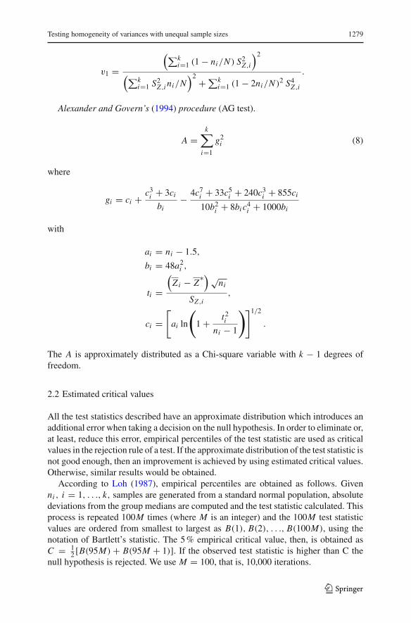
Fig. 1 Type I error rate of Bartlett’s test (B) and Bartlett’s test with kurtosis adjustment (B2)
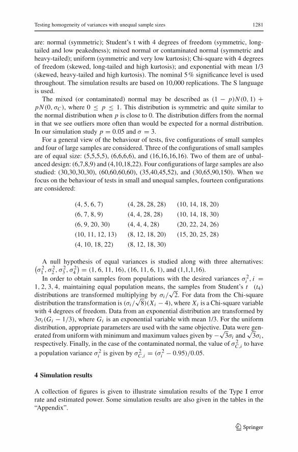
Fig. 2 Type I error rates of tests of group A using the Keyes–Levy adjustment
Power levels are very high for all tests if samples sizes are large, except whenthere are outliers (mixed normal distribution). In this case none of the tests have anacceptable power level under any condition. In contrast, Type I error rates may becontrolled by some of the tests.
With respect to the Type I error rate, the simulation results show that B and B2 testshave their own behavior (see Fig. 1) and the remaining tests may be classified into twogroups with similar performance. Group A would be included by the W(KL), J1(KL),J2(KL) and AG(KL) tests (see Figs. 2, 3, 4, 5), and group B by the L50(KL), BF(KL)and BFR(KL) tests (see Figs. 6, 7, 8, 9).
B test is extremely sensitive to non-normality, as reported in the literature. Havinglarge samples does not lead to control of the Type I error rate under any distribution.However, B2 test is always robust at the significance level and powerful in large samplesizes, except when there are outliers. In small samples, the empirical Type I error rateof B2 test verifies Bradley’s liberal criterion if distributions are symmetric and bell-shaped. Liberality problems are found for the uniform distribution and asymmetricdistributions.
123
Testing homogeneity of variances with unequal sample sizes 1283
Fig. 4 Type I error rates of tests of group A using the Keyes–Levy adjustment and estimated critical values
Type I error rate
0.000
0.025
0.050
0.075
0.100
0.125
5,5,
5,5
6,6,
6,6
16,1
6,16
,16
6,7,
8,9
4,10
,18,
22
30,3
0,30
,30
60,6
0,60
,60
35,4
0,45
,52
30,6
5,90
,150
5,
5,5,
56,
6,6,
616
,16,
16,1
66,
7,8,
9 4,
10,1
8,22
30
,30,
30,3
060
,60,
60,6
035
,40,
45,5
2 30
,65,
90,1
50
5,5,
5,5
6,6,
6,6
16,1
6,16
,16
6,7,
8,9
4,10
,18,
22
30,3
0,30
,30
60,6
0,60
,60
35,4
0,45
,52
30,6
5,90
,150
5,
5,5,
56,
6,6,
616
,16,
16,1
66,
7,8,
9 4,
10,1
8,22
30
,30,
30,3
060
,60,
60,6
035
,40,
45,5
2 30
,65,
90,1
50
5,5,
5,5
6,6,
6,6
16,1
6,16
,16
6,7,
8,9
4,10
,18,
22
30,3
0,30
,30
60,6
0,60
,60
35,4
0,45
,52
30,6
5,90
,150
5,
5,5,
56,
6,6,
616
,16,
16,1
66,
7,8,
9 4,
10,1
8,22
30
,30,
30,3
060
,60,
60,6
035
,40,
45,5
2 30
,65,
90,1
50
Normal Student’s t Mixed-Normal Uniform Chi square Exponential
W(NG)e J(NG)eAG(NG)e
Fig. 5 Type I error rates of tests of group A using the Noguchi–Gel procedure and estimated critical values
Tests in group A: W(KL), J1(KL), J2(KL) and AG(KL). In large sample sizes allof them seem to control the Type I error rate. Serious problems are found in smallsample sizes. In this case if they are equal and odd then tests are too conservative
Fig. 8 Type I error rates of tests of group B using the Keyes–Levy adjustment and estimated critical values
(Fig. 2). This problem disappears (Fig. 3) when structural zeros are removed, buttests still present problems in controlling the Type I error rate. The Type I error rateis under control if decisions are based on estimated critical values and distributionsare symmetric (Fig. 4). Problems of liberality seem to get worse as the degree ofasymmetry increases. Removing structural zeros (Noguchi–Gel procedure) and usingestimated critical values simultaneously lead to a slight improvement (Fig. 5).
123
Testing homogeneity of variances with unequal sample sizes 1285
Type I error rate
0.000
0.025
0.050
0.075
0.1005,
5,5,
56,
6,6,
616
,16,
16,1
66,
7,8,
9 4,
10,1
8,22
30
,30,
30,3
060
,60,
60,6
035
,40,
45,5
2 30
,65,
90,1
50
5,5,
5,5
6,6,
6,6
16,1
6,16
,16
6,7,
8,9
4,10
,18,
22
30,3
0,30
,30
60,6
0,60
,60
35,4
0,45
,52
30,6
5,90
,150
5,
5,5,
56,
6,6,
616
,16,
16,1
66,
7,8,
9 4,
10,1
8,22
30
,30,
30,3
060
,60,
60,6
035
,40,
45,5
2 30
,65,
90,1
50
5,5,
5,5
6,6,
6,6
16,1
6,16
,16
6,7,
8,9
4,10
,18,
22
30,3
0,30
,30
60,6
0,60
,60
35,4
0,45
,52
30,6
5,90
,150
5,
5,5,
56,
6,6,
616
,16,
16,1
66,
7,8,
9 4,
10,1
8,22
30
,30,
30,3
060
,60,
60,6
035
,40,
45,5
2 30
,65,
90,1
50
5,5,
5,5
6,6,
6,6
16,1
6,16
,16
6,7,
8,9
4,10
,18,
22
30,3
0,30
,30
60,6
0,60
,60
35,4
0,45
,52
30,6
5,90
,150
Normal Student’s t Mixed-Normal Uniform Chi square Exponential
L50(NG)e BF(NG)e
Fig. 9 Type I error rates of tests of group B using the Noguchi–Gel procedure and estimated critical values
Estimated power
0.000
0.100
0.200
0.300
0.400
0.500
0.600
0.700
0.800
0.900
1.000
5,5,
5,5
6,6,
6,6
16,1
6,16
,16
6,7,
8,9
4,10
,18,
22
5,5,
5,5
6,6,
6,6
16,1
6,16
,16
6,7,
8,9
4,10
,18,
22
5,5,
5,5
6,6,
6,6
16,1
6,16
,16
6,7,
8,9
4,10
,18,
22
30,3
0,30
,30
60,6
0,60
,60
35,4
0,45
,52
30,6
5,90
,150
5,5,
5,5
6,6,
6,6
16,1
6,16
,16
6,7,
8,9
4,10
,18,
22
5,5,
5,5
6,6,
6,6
16,1
6,16
,16
6,7,
8,9
4,10
,18,
22
5,5,
5,5
6,6,
6,6
16,1
6,16
,16
6,7,
8,9
4,10
,18,
22
a b a b a b a c a c a b a b a b a c a c a b a b a b a c a c a b a b a c a c a b a b a b a c a c a b a b a b a c a c a b a b a b a c a c
Tests in group B: L50(KL), BF(KL) and BFR(KL). They also perform well inlarge sample sizes. However, in small samples they are too conservative in twocases (Fig. 6): (1) when sample sizes are small, equal and odd [for example,(n1, n2, n3, n4) = (5, 5, 5, 5)]; (2) when they are unequal and very small [e.g.(n1, n2, n3, n4) = (6, 7, 8, 9)]. The latter seems to be only applicable in symmet-ric distributions.
Removing structural zeros (Noguchi–Gel procedure) does not lead to controllingthe Type I error rate (Fig. 7). The use of estimated critical values seems to improveperformance but problems of control are observed in highly asymmetric distributionsand in the sample size combination (5,5,5,5) for the uniform distribution (Fig. 8).These results are only improved when both refinements are used (Fig. 9). In this case,both the L50(NG)e and BF(NG)e tests show a very good performance. They controlthe Type I error rate in any of the settings considered in this simulation study (Fig. 10).
Fig. 12 Type I error rates of tests of group A in small sample sizes using the Noguchi–Gel procedure andestimated critical values
Estimated power of heteroscedastic tests
0
0.1
0.2
0.3
0.4
0.5
0.6
0.7
0.8
0.9
1
4,5,
6,7
6,7,
8,9
6,9,
20,3
0
10,1
1,12
,13
4,10
,18,
22
4,28
,28,
28
4,4,
28,2
8
4,4,
4,28
8,12
,18,
20
8,12
,18,
30
10,1
4,18
,20
10,1
4,18
,30
20,2
2,24
,26
15,2
0,25
,28
4,5,
6,7
6,7,
8,9
6,9,
20,3
0
10,1
1,12
,13
4,10
,18,
22
4,28
,28,
28
4,4,
28,2
8
4,4,
4,28
8,12
,18,
20
8,12
,18,
30
10,1
4,18
,20
10,1
4,18
,30
20,2
2,24
,26
15,2
0,25
,28
4,5,
6,7
6,7,
8,9
6,9,
20,3
0
10,1
1,12
,13
4,10
,18,
22
4,28
,28,
28
4,4,
28,2
8
4,4,
4,28
8,12
,18,
20
8,12
,18,
30
10,1
4,18
,20
10,1
4,18
,30
20,2
2,24
,26
15,2
0,25
,28
4,5,
6,7
6,7,
8,9
6,9,
20,3
0
10,1
1,12
,13
4,10
,18,
22
4,28
,28,
28
4,4,
28,2
8
4,4,
4,28
8,12
,18,
20
8,12
,18,
30
10,1
4,18
,20
10,1
4,18
,30
20,2
2,24
,26
15,2
0,25
,28
4,5,
6,7
6,7,
8,9
6,9,
20,3
0
10,1
1,12
,13
4,10
,18,
22
4,28
,28,
28
4,4,
28,2
8
4,4,
4,28
8,12
,18,
20
8,12
,18,
30
10,1
4,18
,20
10,1
4,18
,30
20,2
2,24
,26
15,2
0,25
,28
4,5,
6,7
6,7,
8,9
6,9,
20,3
0
10,1
1,12
,13
4,10
,18,
22
4,28
,28,
28
4,4,
28,2
8
4,4,
4,28
8,12
,18,
20
8,12
,18,
30
10,1
4,18
,20
10,1
4,18
,30
20,2
2,24
,26
15,2
0,25
,28
a b a b a b a b a b a b a b a b a b a b a b a b a b a b a b a b a b a b a b a b a b a b a b a b a b a b a b a b a b a b a b a b a b a b a b a b a b a b a b a b a b a b a b a b a b a b a b a b a b a b a b a b a b a b a b a b a b a b a b a b a b a b a b a b a b a b a b a b a b a b a b a b a b a b a b a b a b a b a b a b a b a b a b a b
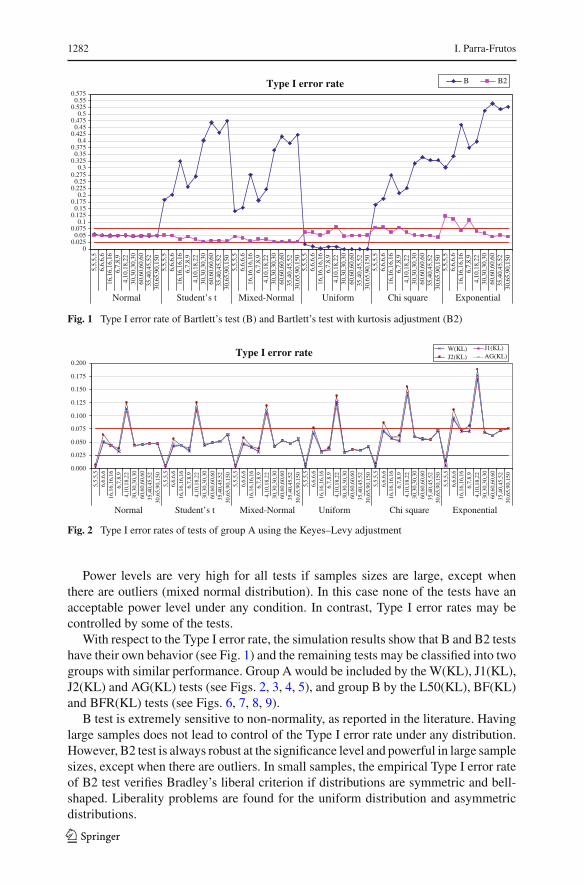
Fig. 13 Estimated power of heteroscedastic tests, Note: a = (σ 21 , σ 2
2 , σ 23 , σ 2
4 ) = (1, 6, 11, 16); b =(16, 11, 6, 1)
To gain further insights into the behaviour of tests in small samples, a new simulationhas been made with a greater variety of small and unequal sample sizes (see Figs. 11,12, 13, and Tables 1, 2 in the “Appendix”). The simulation results indicate that theBF(NG)e and L50(NG)e tests control the Type I error rate in small sample sizes(Fig. 11). However, the BF(NG)e test seems to show a better control than the L50(NG)e
123
Testing homogeneity of variances with unequal sample sizes 1287
Estimated power
0
0.1
0.2
0.3
0.4
0.5
0.6
0.7
0.8
0.9
1
4,5,
6,7
6,7,
8,9
6,9,
20,3
0
10,1
1,12
,13
4,10
,18,
22
4,28
,28,
28
4,4,
28,2
8
4,4,
4,28
8,12
,18,
20
8,12
,18,
30
10,1
4,18
,20
10,1
4,18
,30
20,2
2,24
,26
15,2
0,25
,28
4,5,
6,7
6,7,
8,9
6,9,
20,3
0
10,1
1,12
,13
4,10
,18,
22
4,28
,28,
28
4,4,
28,2
8
4,4,
4,28
8,12
,18,
20
8,12
,18,
30
10,1
4,18
,20
10,1
4,18
,30
20,2
2,24
,26
15,2
0,25
,28
4,5,
6,7
6,7,
8,9
6,9,
20,3
0
10,1
1,12
,13
4,10
,18,
22
4,28
,28,
28
4,4,
28,2
8
4,4,
4,28
8,12
,18,
20
8,12
,18,
30
10,1
4,18
,20
10,1
4,18
,30
20,2
2,24
,26
15,2
0,25
,28
4,5,
6,7
6,7,
8,9
6,9,
20,3
0
10,1
1,12
,13
4,10
,18,
22
4,28
,28,
28
4,4,
28,2
8
4,4,
4,28
8,12
,18,
20
8,12
,18,
30
10,1
4,18
,20
10,1
4,18
,30
20,2
2,24
,26
15,2
0,25
,28
4,5,
6,7
6,7,
8,9
6,9,
20,3
0
10,1
1,12
,13
4,10
,18,
22
4,28
,28,
28
4,4,
28,2
8
4,4,
4,28
8,12
,18,
20
8,12
,18,
30
10,1
4,18
,20
10,1
4,18
,30
20,2
2,24
,26
15,2
0,25
,28
4,5,
6,7
6,7,
8,9
6,9,
20,3
0
10,1
1,12
,13
4,10
,18,
22
4,28
,28,
28
4,4,
28,2
8
4,4,
4,28
8,12
,18,
20
8,12
,18,
30
10,1
4,18
,20
10,1
4,18
,30
20,2
2,24
,26
15,2
0,25
,28
a b a b a b a b a b a b a b a b a b a b a b a b a b a b a b a b a b a b a b a b a b a b a b a b a b a b a b a b a b a b a b a b a b a b a b a b a b a b a b a b a b a b a b a b a b a b a b a b a b a b a b a b a b a b a b a b a b a b a b a b a b a b a b a b a b a b a b a b a b a b a b a b a b a b a b a b a b a b a b a b a b a b a b a b
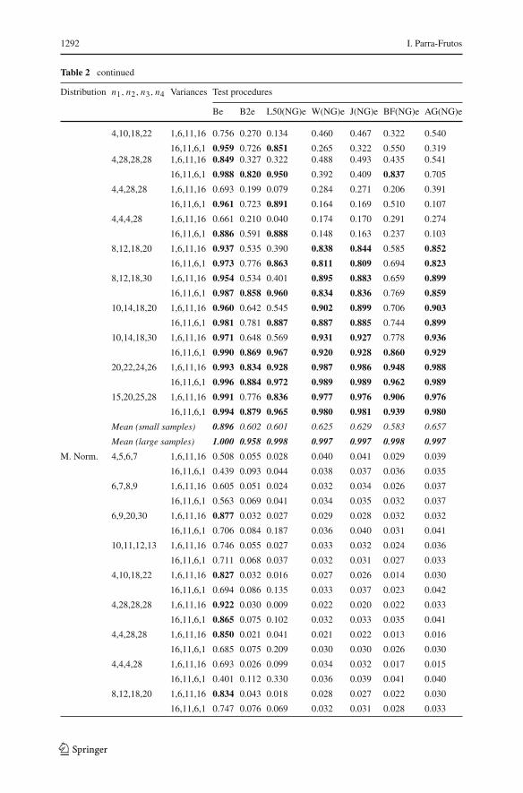
test. In small and unequal sample sizes problems of heteroscedasticity of Zi j andZi j/κni may appear, so a heteroscedastic test is expected to perform better. However,the degree of heteroscedasticity may not be too high when σ 2
i , i = 1, . . ., 4, are equal(the largest variance is 1.45 times the smaller one and is associated to the small samplesize) as to give rise to serious problems of liberality when applying the homoscedasticLevene test L50(NG)e. Simulation results seem to confirm this extent (see Fig. 11).On the other hand, asymmetry and negative (or positive) correlation between samplesizes and population variances are problems for tests comparing means, the BF(NG)etest seems to be the most robust in these situations.
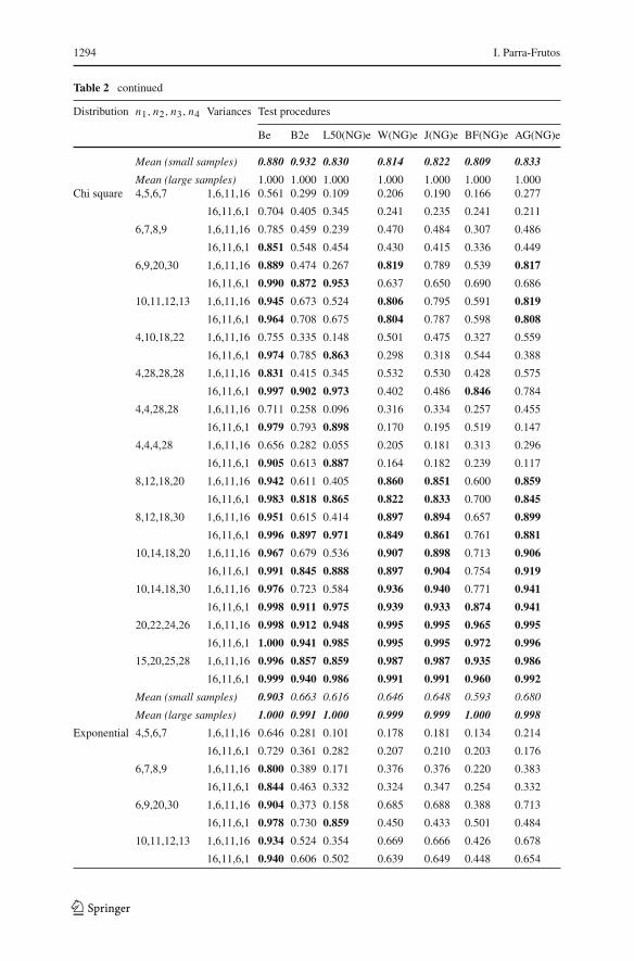
Power is slightly lower for the BF(NG)e test than for the remaining heteroscedastictests (Fig. 13). This would suggest using W(NG)e, J(NG)e or AG(NG)e except whendistributions are highly asymmetric (like the exponential distribution). For highlyasymmetric distributions the BF(NG)e test shows a better control of the Type I errorrate than the L50(NG)e test. However, the L50(NG)e test is more powerful than theBF(NG)e test when the unknown population variances σ 2
i are negatively correlatedwith the sample sizes (Fig. 14).
Simulation results also show that tests have a very low power when there are outliers,although they may control the Type I error rate (Figs. 11, 13).
5 Conclusions
Problems of heteroscedasticity of the variables given by the absolute deviation fromthe median arise when sample sizes are unequal. To deal with the heterogeneity ofthese variables in Levene’s test we propose substituting the ANOVA step for a het-eroscedastic alternative. We focus on tests given by Welch (1951), James (1951),Brown and Forsythe (1974b), Rubin (1983) and Mehrotra (1997)—a correction to theBrown–Forsythe test, and Alexander and Govern (1994). The Keyes–Levy adjustmentconsisting of dividing the observations by κni is applied to get the correct null hypoth-esis of equal variances. We also consider removing structural zeros, according to theNoguchi–Gel procedure, and using estimated critical values.
None of the tests considered in this study show a good performance when thereare outliers. In this case, the Type I error rate may be controlled by tests when usingestimated critical values, but power levels are always too low.
123
1288 I. Parra-Frutos
Removing structural zeros implies a substantial improvement in the tests, buta better performance is achieved when estimated critical values are also applied.Moreover, simulation results show that for the variables Zi j/κni the heteroscedas-tic tests perform better than the ANOVA step used by Levene’s test in small andunequal sample sizes. In particular, the Brown–Forsythe test (BF(NG)e test) con-trols the Type I error rate in all settings studied here. The L50(NG)e test alsoseems to be robust to nominal significant level according to Bradley’s criterion.However, only the empirical Type I error rate of the BF(NG)e test falls withinthe narrower interval [0.035, 0.065]. The James (J(NG)e), Alexander and Govern(AG(NG)e), and Welch (W(NG)e) tests show a good performance even in asym-metric distributions like the chi square, but they do not control the Type I errorrate in highly asymmetric distributions, like the exponential. Nevertheless, they areslightly more powerful than the BF(NG)e test. In large samples, heteroscedastic tests(BF(NG)e, W(NG)e, J(NG)e and AG(NG)e) and Levene’s test (L50(NG)e) performsimilarly.
In conclusion, according to the results obtained in the simulation study, in small andunequal sample sizes it is recommendable to use W(NG)e, J(NG)e or AG(NG)e testswhen testing homoscedasticity whenever the distributions are not highly asymmetric,otherwise the BF(NG)e test is preferable. The L50(NG)e test may be liberal.
Acknowledgments The author is sincerely grateful to two anonymous referees and the Associate Editorfor their time and effort in providing very constructive, helpful and valuable comments and suggestions thathave led to a substantial improvement in the quality of the paper.
6 Appendix
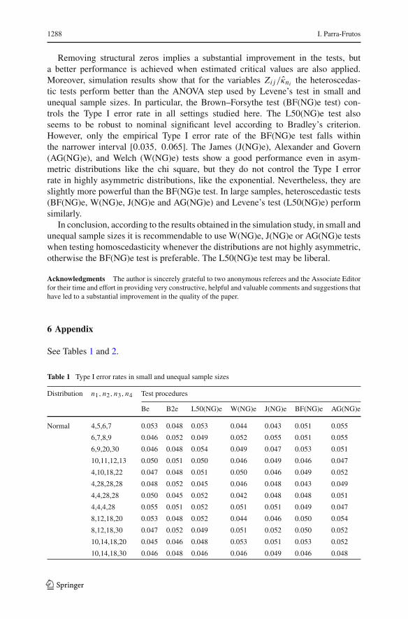
See Tables 1 and 2.
Table 1 Type I error rates in small and unequal sample sizes
Distribution n1, n2, n3, n4 Test procedures
Be B2e L50(NG)e W(NG)e J(NG)e BF(NG)e AG(NG)e
Normal 4,5,6,7 0.053 0.048 0.053 0.044 0.043 0.051 0.055
Mean (small samples) 0.907 0.546 0.507 0.547 0.550 0.465 0.572
Mean (large samples) 1.000 0.961 0.994 0.992 0.992 0.995 0.990
Structural zeros are removed and critical values are estimatedEstimated power levels larger than 0.8 are in bold
References
Akritas MG, Papadatos N (2004) Heteroscedastic one-way ANOVA and lack-of-fit tests. J Am Stat Assoc99:368–382
Alexander RA, Govern DM (1994) A new and simpler approximation and ANOVA under variance hetero-geneity. J Educ Stat 19:91–101
Bartlett MS (1937) Properties of sufficiency and statistical tests. Proc R Soc Lond A Mat A 160:268–282Bathke A (2004) The ANOVA F test can still be used in some balanced designs with unequal variances and
nonnormal data. J Stat Plan Inference 126:413–422Boos DD, Brownie C (1989) Bootstrap methods for testing homogeneity of variances. Technometrics
31:69–82Boos DD, Brownie C (2004) Comparing variances and other measures of dispersion. Stat Sci 19:571–578Box GEP (1954) Some theorems on quadratic forms applied in the study of analysis of variance problems.
I. Effect of inequality of variance in the one-way classification. Ann Math Stat 25:290–302Bradley JV (1978) Robustness? Br J Math Stat Psych 31:144–152Brown MB, Forsythe AB (1974a) Robust tests for equality of variances. J Am Stat Assoc 69:364–
367
123
1296 I. Parra-Frutos
Brown MB, Forsythe AB (1974b) The small sample behavior of some statistics which test the equality ofseveral means. Technometrics 16:129–132
Cahoy DO (2010) A bootstrap test for equality of variances. Comput Stat Data Anal 54:2306–2316Carroll RJ, Schneider H (1985) A note on Levene’s test for equality of variances. Stat Probab Lett 3:191–194Charway H, Bailer AJ (2007) Testing multiple-group variance equality with randomization procedures.
J Stat Comput Simul 77:797–803Clinch JJ, Keselman HJ (1982) Parametric alternatives to the analysis of variance. J Educ Stat 7:207–214Cochran WG (1954) Some methods for strengthening the common χ2-tests. Biometrics 10:417–451Conover WJ, Johnson ME, Johnson MM (1981) A comparative study of tests for homogeneity of variances,
with applications to the outer continental shelf bidding data. Technometrics 23:351–361De Beuckelaer A (1996) A closer examination on some parametric alternatives to the ANOVA F-test. Stat
Pap 37:291–305Dijkstra JB, Werter PS (1981) Testing the equality of several means when the population variances are
unequal. Commun Stat B-Simul 10:557–569Glass GV, Peckham PD, Sanders JR (1972) Consequences of failure to meet assumptions underlying the
fixed effects analyses of variance and covariance. Rev Educ Res 42:237–288Harwell MR, Rubinstein EN, Hayes WS, Olds CC (1992) Summarizing Monte Carlo results in method-
ological research: the one- and two-factor fixed effects ANOVA cases. J Educ Stat 17:315–339Hui W, Gel YR, Gastwirth JL (2008) lawstat: an R package for law, public policy and biostatistics. J Stat
Softw 28. http://www.jstatsoft.org/v28/i03/paperHines WGS, O’Hara Hines RJ (2000) Increased power with modified forms of the Levene (Med) test for
heterogeneity of variance. Biometrics 56:451–454Hsiung T, Olejnik S, Huberty CJ (1994) Comment on a Wilcox test statistic for comparing means when
variances are unequal. J Educ Stat 19:111–118Iachine I, Petersen HC, Kyvikc KO (2010) Robust tests for the equality of variances for clustered data.
J Stat Comput Simul 80:365–377James GS (1951) The comparison of several groups of observations when the ratios of the population
variances are unknown. Biometrika 38:324–329Johansen S (1980) The Welch-James approximation of the distribution of the residual sum of squares in
weighted linear regression. Biometrika 67:85–92Kenny DA, Judd CM (1986) Consequences of violating the independence assumption in analysis of variance.
Psychol Bull 99:422–431Keselman HJ, Rogan JC, Feir-Walsh BJ (1977) An evaluation of some nonparametric and parametric tests
for location equality. Br J Math Stat Psychol 30:213–221Keselman HJ, Wilcox RR, Algina J, Othman AR, Fradette K (2008) A comparative study of robust tests
for spread: Asymmetric trimming strategies. Br J Math Stat Psychol 61:235–253Keyes TK, Levy MS (1997) Analysis of Levene’s test under design imbalance. J Educ Behav Stat 22:
227–236Layard MWJ (1973) Robust large-sample tests for homogeneity of variances. J Am Stat Assoc 68:195–198Levene H, Levene H (1960) Robust tests for equality of variances. Essays in Honor of Harold Hotelling.
In: Olkin I, Ghurye SG, Hoeffding W, Madow WG, Mann HB (eds) Contributions to probability andstatistics. Stanford University Press, Palo Alto, p 292
Lim TS, Loh WY (1996) A comparison of tests of equality of variances. Comput Stat Data Anal 22:287–301Lix LM, Keselman JC, Keselman HJ (1996) Consequences of assumption violations revisited, a quantitative
review of alternatives to the one-way analysis of variance F test. Rev Educ Res 66:579–619Loh WY (1987) Some modifications of Levene’s test of variance homogeneity. J Stat Comput Simul
28:213–226Markowski CA, Markowski EP (1990) Conditions for the effectiveness of a preliminary test of variance.
Am Stat 44:322–326Mehrotra DV (1997) Improving the Brown-Forsythe solution to the generalizied Behrens-Fisher problem.
Commun Stat-Simul 26:1139–1145Neuhäuser M (2007) A comparative study of nonparametric two-sample tests after Levene’s transformation.
J Stat Comput Simul 77:517–526Neuhäuser M, Hothorn LA (2000) Location-scale and scale trend tests based on Levene’s transformation.
Comput Stat Data Anal 33:189–200Noguchi K, Gel YR (2010) Combination of Levene-type tests and a finite-intersection method for testing
equality of variances against ordered alternatives. J Nonparametr Stat 22:897–913
Testing homogeneity of variances with unequal sample sizes 1297
O’Neill ME, Mathews K (2000) A weighted least squares approach to Levene’s test of homogeneity ofvariance. Aust Nz J Stat 42:81–100
Oshima TC, Algina J (1992) Type I error rates for James’s second-order test and Wilcox’s Hm test underheteroscedasticity and non-normality. Br J Math Stat Psychol 45:255–263
Parra-Frutos I (2009) The behaviour of the modified Levene’s test when data are not normally distributed.Comput Stat 24:671–693
Rogan JC, Keselman HJ (1977) Is the ANOVA F-test robust to variance heterogeneity when samples sizesare equal? Am Educ Res J 14:493–498
Rubin AS (1983) The use of weighted contrasts in analysis of models with heterogeneity of variance. P BusEco Stat Am Stat Assoc 347–352
Scheffé H (1959) The analysis of variance. Wiley, New YorkSchneider PJ, Penfield DA (1997) Alexander and Govern’s approximation, providing an alternative to
ANOVA under variance heterogeneity. J Exp Educ 65:271–286Siegel S, Tukey JW (1960) A nonparametric sum of ranks procedure for relative spread in unpaired samples.
J Am Stat Assoc 55:429–444 (corrections appear in vol. 56:1005)Welch BL (1951) On the comparison of several mean values, an alternative approach. Biometrika 38:
330–336Wilcox RR (1988) A new alternative to the ANOVA F and new results on James’ second-order method.
Br J Math Stat Psychl 41:109–117Wilcox RR (1989) Adjusting for unequal variances when comparing means in one-way and two-way fixed
effects ANOVA models. J Educ Stat 14:269–278Wilcox RR (1990) Comparing the means of two independent groups. Biom J 32:771–780Wilcox RR (1995) ANOVA: a paradigm for low power and misleading measures of effect size? Rev Educ
Res 65:51–77Wilcox RR (1997) A bootstrap modification of the Alexander-Govern ANOVA method, plus comments on
comparing trimmed means. Educ Psychol Meas 57:655–665Wilcox RR, Charlin VI, Thompson KL (1986) New Monte Carlo results on the robustness of the ANOVA
F, W and F-statistics. Commun Stat Simul C 15:933–943Wludyka P, Sa P (2004) A robust I-sample analysis of means type randomization test for variances for
unbalanced designs. J Stat Comput Simul 74:701–726


![Betere marketing dank zij een marketingplan [summary]](https://static.documents.pub/doc/80x56/5498763eac79590e2e8b5653/betere-marketing-dank-zij-een-marketingplan-summary.jpg)


