66
Working Paper No. 571 Arun G. Chandrasekhar | Horacio Larreguy | Juan Pablo Xandri May 2016 Testing Models of Social Learning on Networks: Evidence from a Lab Experiment in the Field

Working Paper No. 571
Arun G. Chandrasekhar | Horacio Larreguy | Juan Pablo Xandri
May 2016
Testing Models of Social Learning on Networks: Evidence from a Lab
Experiment in the Field

TESTING MODELS OF SOCIAL LEARNING ON NETWORKS:EVIDENCE FROM A LAB EXPERIMENT IN THE FIELD
ARUN G. CHANDRASEKHAR‡, HORACIO LARREGUY§, AND JUAN PABLO XANDRI?
Abstract. Agents often use noisy signals from their neighbors to update their beliefsabout a state of the world. The effectiveness of social learning relies on the details of howagents aggregate information from others. There are two prominent models of informationaggregation in networks: (1) Bayesian learning, where agents use Bayes’ rule to assess thestate of the world and (2) DeGroot learning, where agents instead consider a weightedaverage of their neighbors’ previous period opinions or actions. Agents who engage inDeGroot learning often double-count information and may not converge in the long run.We conduct a lab experiment in the field with 665 subjects across 19 villages in Karnataka,India, designed to structurally test which model best describes social learning. Sevensubjects were placed into networks with common knowledge of the network structure,designed to maximize our experimental power to distinguish between these two models oflearning. Subjects attempted to learn the underlying (binary) state of the world, havingreceived independent identically distributed signals in the first period. Thereafter, ineach period, subjects made guesses about the state of the world, and these guesses weretransmitted to their neighbors at the beginning of the following round. We structurallyestimate a model of Bayesian learning, relaxing common knowledge of Bayesian rationalityby allowing agents to have incomplete information about other players’ types (Bayesianor DeGroot updating types). Our estimates show that, despite the flexibility in modelinglearning in these networks, agents are robustly best described by DeGroot-learning modelswherein they take a simple majority of previous guesses in their neighborhood.
Keywords: networks, social learning, Bayesian learning, DeGroot learning, experi-ments
JEL Classification Codes: D83, C92, C91, C93
1. Introduction
The way in which individuals aggregate information is a critical feature of many eco-nomic environments. Information and opinions about new technologies, job opportunities,
Date: First Version: August 2011, This Version: May 2016.We are grateful to Daron Acemoglu, Abhijit Banerjee, Esther Duflo, Ben Golub, Matthew O. Jackson,Markus Möbius, and Adam Szeidl for extremely helpful discussions. Essential feedback was provided byKalyan Chatterjee, Juan Dubra, Rema Hanna, Ben Olken, Evan Sadler, Rob Townsend, Xiao Yu Wang,Luis Zermeño and participants at numerous seminars and conferences. We also thank Mounu Prem forexcellent research assistance. This project was possible thanks to the financial support of the Russell SageBehavioral Economics Grant. Chandrasekhar is grateful for support from the National Science FoundationGFRP. Larreguy thanks the Bank of Spain and Caja Madrid for financial support. JPAL and CMF atIFMR provided valuable logistical assistance. Gowri Nagraj and our field team were vital to the project’sprogress. All errors are our own.‡Stanford University, Department of Economics and NBER.§Harvard University, Department of Government.?Princeton University, Department of Economics.
1

TESTING MODELS OF SOCIAL LEARNING ON NETWORKS 2
products, and political candidates, among other things, are largely transmitted throughsocial networks. However, the information individuals receive from others about the stateof the world often contain noise. Moreover, individuals might differ in how they imaginethat others interpret and process information they retransmit. A critical aspect of sociallearning, therefore, concerns how agents handle and aggregate noisy information in or-der to resolve uncertainty and estimate the state of the world, on which they base theirsubsequent decisions.
Consider the case where an individual A hears which of two choices each of her twofriends B and C intend to make in the coming period. For example, this could be which oftwo fertilizers her friends intend to use or which of two candidates her friends are likely tovote for. Both B and C have friends of their own, including some shared friends, and havediscussed their choices with them. Knowing all of this, when A updates her opinion as towhich choice is best, how should she incorporate B’s and C’s views? She may naively treatthem as independent clues about the optimal choice, or perhaps she is more sophisticatedand worries that there is a common component to their opinions because they have friendsin common. Or A may even worry about how B and C themselves make inferences aboutthe world, and thus, arrive at their opinions. In this paper, we conduct a lab experimentin the field in order to carefully study the nature of social learning on a network, focusingon the two canonical models in the learning on networks literature: Bayesian and DeGrootlearning (Jackson, 2008; Acemoglu et al., 2011; Choi et al., 2015). Relative to existingliterature, our main contribution is that we allow for incomplete information by agentsabout other agents’ types, and thus we do not simply restrict to the race between completeinformation Bayesian and DeGroot learning, allowing then a fair comparison between thetwo learning models.
There are two broad paradigms of modeling social learning through networks. The firstis Bayesian learning, wherein individuals process information using Bayes’ rule (see, e.g.,Banerjee (1992), Bikhchandani, Hirshleifer, and Welch (1992), Gale and Kariv (2003),Acemoglu, Dahleh, Lobel, and Ozdaglar (2011), Mossel and Tamuz (2010), Lobel andSadler (forthcoming)). An environment often studied considers a situation where eachindividual initially receives a signal about the state of the world and then subsequentlyobserves her neighbors’ guesses, before revising her own belief and offering an updatedguess in each period. A core result in this setting is that individuals eventually convergein their beliefs as to which state of the world they are in; this guess is correct in largenetworks when some regularity conditions hold (Gale and Kariv, 2003; Mossel and Tamuz,2010). While Bayesian agents in large networks are able to come to the right opinion in thisenvironment, these results rely on sophisticated agents who are able to implicitly discernbetween repeated and new information that they receive through their neighbors over time.
This cognitive load that the Bayesian-learning model imposes over agents when theselearn in social networks led to a second paradigm: DeGroot learning (DeGroot, 1974). In
TESTING MODELS OF SOCIAL LEARNING ON NETWORKS 3
these models, agents are myopic and, after seeing the behavior or beliefs of their networkneighbors, they take a weighted average of these to construct their belief going into thesubsequent period. Ellison and Fudenberg (1993; 1995), DeMarzo, Vayanos, and Zwiebel(2003), Eyster and Rabin (2010; 2014), Golub and Jackson (2010), and Jadbabaie, Molavi,Sandroni, and Tahbaz-Salehi (2012) among others, have studied related models of thisform. When agents communicate beliefs with their neighbors and engage in DeGrootlearning they converge to the truth in large networks (Golub and Jackson, 2010). However,this convergence can be inefficient and agents located in networks that exhibit significanthomophily – wherein agents tend to be connected more with similar others – convergeslowly to the truth (Golub and Jackson, 2012).1
The contrast between DeGroot and Bayesian learning grows when one moves away fromrich communication structures – where agents exchange beliefs with their neighbors – inDeGroot learning models.2 In many environments of interest, communication can be farmore coarse: individuals might reveal which candidate they voted for but are probablyless willing to discuss the reasons (e.g., underlying beliefs about candidate competence)behind such vote choice, farmers might observe which fertilizer their neighboring farmersadopted but struggle to elicit from them what fertilizer quality considerdations led themto such fertilizer choice, individuals might observe their neighbors joining a microfinanceorganization but their neighbors might struggle to communicate the motives behind suchtake up. Moreover, and perhaps especially in a context such as ours where education levelsare low, assuming that fine probabilities and complex beliefs are communicated by agentsmay be unrealistic. It is unsurprising then that much of the Bayesian learning on networksliterature focuses on coarse communication, where agents observe their neighbors’ actionsas opposed to their beliefs. The differences between the Bayesian and DeGroot paradigmsare particularly pronounced in these environments. While Bayesian learning typicallygenerates convergence to the truth in large societies under certain regularity conditions,DeGroot learning may generate misinformation traps, wherein pockets of agents hang onto an incorrect opinion for infinitely many periods. Thus, understanding which learningparadigm better predicts group behavior is important both for understanding whetherinformation transmission is efficient and for thinking through policy designs that rely oninformation dissemination.3
1Eyster and Rabin (2014) also restrict to a continuous action space that fully reveals players’ posteriorbeliefs but consider larger class of behaviors than DeGroot-style behavior. They show that players thatuse social learning rules that neglect redundancy can converge to wrong long-run beliefs with positiveprobability. They conclude that abundant imitation might be socially harmful.2For a recent review article, see Sadler (2014).3Consider the case where the state of the world is either 0 or 1. In this binary environment, individualsengaging in DeGroot learning often double-count information, fail to not take into account dependencies,and may not reach consensus in the long run even for extremely large graphs (as we show below). Meanwhile,in such an environment, Bayesian learning mechanisms, under some regularity conditions to avoid ties inposterior probabilities, generically generate consensus in finite graphs and, moreover, in very large graphs

TESTING MODELS OF SOCIAL LEARNING ON NETWORKS 4
In this paper, we study whether Bayesian or DeGroot learning does a better job ofdescribing learning on networks. We conducted a unique lab experiment in the field in 19villages in rural Karnataka, India, with 665 subjects. We ran our experiments directly inthe villages so that we could study a population of interest to development economists andpolicy makers – namely, those who could be potentially targeted by policy that depends onsocial learning (e.g., the introduction of a new technology, health practices, microfinance).We designed simple networks that maximized statistical power to distinguish between thetwo canonical models in the learning on networks literature: Bayesian and DeGroot learning(Choi et al., 2015). We then conducted a lab experiment in the field, using these networks tostructurally study which cannonical learning model better fits learning in social networks.The network selection was at the conscious potential cost of not being able to separatebetween other models of social learning studied in the literature and discussed later, butreflected the need to select small but sufficiently large networks to have power to distinguishbetween the two models of learning the literature deems as most relevant (Choi et al., 2015).
We created networks of seven individuals, giving each individual a map of the entiregraph so that the full complete informational structure was comprehended. The underlyingstate of the world was either 1 or 0 with equal probability. At t = 0 each individualreceived an independent identically distributed (i.i.d.) signal about the underlying state ofthe world and was informed that signals were correct with probability 5/7. After receivingthe signal, each individual privately made a guess about the state of the world, which wascommunicated to each individual’s network neighbors. Thereafter, each individual madeguesses about the underlying state of the world, and these guesses were transmitted to herneighbors at the beginning of the following round. Using this information, each individualmade a new guess about the state of the world, which in turn was communicated toeach of her network neighbors at the beginning of the following period. Individuals wereincentivized to guess correctly, as we discuss in further detail below.4
In comparing Bayesian and DeGroot learning, the following subtle issue must be consid-ered. The standard Bayesian-learning model typically encodes two important but distinctfeatures: (1) agents are Bayesian, and therefore apply Bayes’ rule to make inferencesabout neighbors’ information sets; and (2) agents have common knowledge of the ways inwhich their neighbors map information sets to actions. The first condition is that agentsare Bayesian, and the second condition is that they have correct beliefs about the otheragents’ types, i.e., whether they are Bayesian or DeGroot learners. The most extremeversion of this is a model is one of complete information where everyone is Bayesian and
the populations’ limit belief coincides with the true state of the world (Gale and Kariv, 2003; Mossel andTamuz, 2010). That is, if the world was truly 0, all individuals would eventually come to believe this.4While it could be the case that players were extremely sophisticated and engaged in experimentation inearly rounds, anecdotal evidence from participants suggests that this is not the case. In addition, thetheoretical and experimental literature assumes away experimentation (see, e.g., Choi et al. (2012), Mosselet al. (2015)).

TESTING MODELS OF SOCIAL LEARNING ON NETWORKS 5
this is common knowledge. Our approach is unique in that relaxes both of these featureswhen studying the data, and thus allow for a better comparison of Bayesian and DeGrootlearning models. A model of Bayesian agents with common knowledge of Bayes-rationalityis, in a sense, a strawman; Bayesian agents who are uncertain of their neighbors’ types maybehave differently than Bayesian agents who have common knowledge of Bayes-rationalityof their network. We structurally estimate a Bayesian learning model with incomplete in-formation, where agents need not know ex-ante how others are learning, and relax commonknowledge, as well. The key parameter in our incomplete information Bayesian learningmodel is π, which is the share of agents in the population who are Bayesian, with theassumption that a 1 − π share of agents are DeGroot learners in their thinking. We arethen interested in what π ∈ [0, 1] best describes the data from the experiment.
To assess how a particular model fits the experimental data, we look at the data fromtwo different perspectives: the network level and the individual level. The network-levelanalysis considers the entire network and sequence of actions by agents as a single obser-vation. That is, we consider the path of actions predicted by theory under a model ofsocial learning for each individual in each period. This is an important frame for analysisbecause, while all models are wrong, what we are interested in, as researchers studying so-cial networks, is what the learning process better explains the aggregate learning patternsin our experimental data. In the individual-level analysis, instead of focusing on the thesocial network itself as the observational unit, we consider the action of an individual givena history of actions. We then study which learning model better predicts individual-leveldecisions, given a history of observed signal and neighbors’ actions.
Our core results are as follows. Considering first the network-level analysis, we find thatthe incomplete information model that better explains the data is one where the share ofBayesian agents in the population (π) is 0. Thus, the data is best fit by a model whereall agents are DeGroot. Specifically, this model explains between 86% and 88% of the theactions taken in the data. This is not to say that social learning is not well approximatedby Bayesian learning; a complete information Bayesian learning model explains 82% of theexperimental data. However, this fit largely originates from the fact that the predictionsof the Bayesian and DeGroot models often agree. Moreover, Bayesian block bootstrap,which accounts for dependence in the data due to individuals playing the same learn-ing game, indicates that the difference in fit between the DeGroot and Bayesian learningmodels is statistically significant. Second, at the individual level, again we find that in-complete information Bayesian models fit the data better when the proportion of Bayesianagents (π) is 0 and there is common knowledge about this. In fact, the DeGroot-learningmodels explain between 89% and 94% of the actions taken by agents given a history ofactions. Meanwhile, the complete information Bayesian model only explains 74% of thoseactions. Again, the difference in fit between the DeGroot and Bayesian learning models isstatistically significant.

TESTING MODELS OF SOCIAL LEARNING ON NETWORKS 6
We also establish several supplementary results which may also be of independent inter-est. First, we explore the DeGroot action model (also called the voter model) and demon-strate that even in simple networks where Bayesian learners who observe their neighbors’actions and DeGroot agents who fully communicate their beliefs would converge to thetruth, a non-vanishing and non-trivial share of agents could converge to the wrong beliefs.This is important because while Bayesian learning where actions are observed (or coarseinformation is transmitted) is typically studied in the literature, DeGroot learning modelstypically study settings where very fine information is communicated. In our view, the fairanalog of Bayesian learning where actions are observed is DeGroot learning where actionsare observed. It turns out that in this setting, DeGroot-induced errors in learning can de-stroy efficient social learning in networks that would otherwise be asymptotically efficientunder either Bayesian (action) learning or DeGroot communication learning.
Second, we develop a simple, non-parametric test that directly distinguishes betweenDeGroot-like and Bayesian behavior and show that a considerable share of time the datais consistent with an all-agent DeGroot model.
Third, we develop a simple algorithm to compute incomplete information Bayesian learn-ing on networks that is the best network-independent algorithm. Specifically, it is com-putationally tight in the sense that, asymptotically, there can be no faster algorithm thatis independent of network structure. This is a challenge that, to our knowledge, previouswork had not overcome, precluding a structural analysis of learning on networks like ours.Namely, the algorithm is O(T ), where T is the number of rounds played.5
Fourth, an approach taken in related work looks at learning models with trembles or,relatedly, quantal response equilibrium (QRE) a la Choi et al. (2012). We demonstratethat networks small enough to avoid computational constraints are not large enough toseparate between DeGroot and Bayesian learning with trembles. Meanwhile those that arelarge enough to separate between those models become computationally infeasible to studyusing trembles or QRE.
Fifth, we discuss why selecting between DeGroot and Bayesian learning models must bedone through structural estimation and in a lab setting. We show that natural examplesof reduced form analyses, where the intuitions of Bayesian and DeGroot learning are usedto test for predictions in regression analysis of social learning data, may be problematic.Namely, the data generated by Bayesian and DeGroot learning models do not necessarilyconform to the intuition motivating the regressions. Thus, there much to be gained froma structural analysis. The computational constraints for structural estimation of learn-ing models in large networks, however, suggests the importance of small networks in labsettings to separate between models of social learning. Moreover, lab settings allow con-trolling priors of agents in the network and the signal quality, as well as restricting the
5An algorithm is O (T ) if the number of computations as a function of T , f (T ), is such that f(T )T→M for
some constant M . In particular, this is true if f (T ) = MT , as it is in our algorithm.

TESTING MODELS OF SOCIAL LEARNING ON NETWORKS 7
communication among individuals and the social-network structure. Since structural esti-mation is often sensitive to misspecification, it is difficult to cleanly identify which modelbest describes the data in a non-laboratory context.
In terms of related work, Gale and Kariv (2003) study the Bayesian learning environmentthat we build upon. They only focus on Bayesian learning and extend the learning model toa finite social network with multiple periods. At time t, each agent makes a decision givenher information set, which includes the history of actions of each of her neighbors in thenetwork. Via the martingale convergence theorem, they point out that connected networkswith Bayesian agents yield uniform actions in finite time with probability one. Choi et al.(2005, 2012) make a seminal contribution to the empirical literature of social learning bytesting the predictions derived by Gale and Kariv (2003) in a laboratory experiment. Theyare able to show that features of the Bayesian social learning model fit the data well fornetworks of three individuals. Closer to the goal of our paper, Choi (2012) estimates acognitive-hierarchy model of social learning on networks using the experimental data fromChoi et al. (2005) and finds that Bayesian behavior better fits the experimental data.However, note that, while an important step towards our goal, none of these papers studywhether Bayesian orDeGroot learning models better explain the experimental learningbehavior. The networks do not allow for statistical power under the DeGroot alternatives.In extremely simple networks, such as the ones studied in their paper, there are few (if any)differences in the predicted individual learning behavior by the Bayesian and DeGroot-typelearning models.6
The works most closely related to ours are Möbius et al. (2015), conducted in 2004,who study how information decays as it spreads through networks, Corazzini et al. (2012),Mueller-Frank and Neri (2013) and Mengel and Grimm (2014), who conduct lab experi-ments similar to ours. Möbius et al. (2015) test between DeGroot models and an alterna-tive model that they develop in which individuals “tag” information by describing its origin(called a “streams” model). Note that they do not study Bayesian learning alternatives perse, because that would be computationally prohibitive in their setting. Their experimentuses network data from Harvard undergraduates in conjunction with a field experiment andfinds evidence in favor of the “streams” model model in which individuals “tag” informa-tion. In our experiment, we shut down the possibility that individuals “tag” information.This allows us to compare the Bayesian model to DeGroot alternatives since, as describedabove, looking at Bayesian learning even in a complete information context (let alone in-complete information) is impossible in such a field setting. As noted by Möbius et al.(2015), the conclusions of our work and theirs suggest that in complicated environmentswhere tagging can be difficult, agents may exhibit more DeGroot-like learning behavior.
6The literature on social learning experiments begins with Anderson and Holt (1997), Hung and Plott(2001), and Kubler and Weizsacker (2004). Explicit network structures are considered in a series of papersby Gale and Kariv (2003) , Choi et al. (2005, 2012), and Celen et al. (2010).

TESTING MODELS OF SOCIAL LEARNING ON NETWORKS 8
Prior to our work, Corazzini et al. (2012), study one simple network where Bayesian andDeGroot learning models differ in their predictions. They show reduced form experimentalevidence consistent with DeGroot learning. The authors further propose a generalizedupdating rule that nests DeGroot as a special case, and they show that it fits the datawell. However, as (Choi et al., 2015) highlight, Corazzini et al. (2012) only investigate onesimple network in which there is a difference between the outcomes of the Bayesian andDeGroot learning, making it difficult to generalize their findings.7 Moreover, in section 5we show that selecting between Bayesian and DeGroot learning models through reducedform approaches may be problematic. Subsequent to our work, and independently ofus, both Mueller-Frank and Neri (2013) and Mengel and Grimm (2014) conducted labexperiments to look at Bayesian versus DeGroot learning. Like Corazzini et al. (2012),these studies offer some modified models of learning. Mueller-Frank and Neri (2013), forinstance, develop a general class of models called Quasi-Bayesian updating and show thatlong run outcomes in their experiments are consistent with this model. Crucial differencesfrom our work include the fact that Mueller-Frank and Neri (2013) and Mengel and Grimm(2014) don’t reveal the information about the entire network to their subjects, making theinference problem more complicated. More importantly, none of these studies allow for theiragents to have incomplete information, which can greatly change the benchmark Bayesian’sbehavior. We are particularly interested relaxing the complete information Bayesian modelwith common knowledge of Bayesian rationality since, in a sense, it serves as a weak strawman. In theory, with a mix of Bayesian and naive agents, a Bayesian agent understandingthe heteroegeneity in the population would behave in a manner such that the data wouldlook very different from a world in which all agents are Bayesian. Taken together, there is avibrant literature interested in whether learning in networks can be thought of as DeGrootor Bayesian.
The rest of the paper is organized as follows. Section 2 develops the theoretical frame-work. Section 3 contains the experimental setup. Section 4 describes the structural esti-mation procedure and the main results of the estimation. Section 5 presents the discussionof the difficulties of reduced form approaches. Section 6 concludes.
2. Framework
2.1. Setup.
2.1.1. Notation. Let G = (V,E) be a graph with a set V of vertices and E of edges andput n = |V | as the number of vertices. We denote by A = A (G) the adjacency matrix of Gand assume that the network is an undirected, unweighted graph, with Aij = 1 ij ∈ E.
7Brandts et al. (2015) extends the work by Corazzini et al. (2012) showing further experimental evidenceconsistent with DeGroot learning considering other networks. However, the simple networks they considerdo not allow for statistical power to distinguish between Bayesian and DeGroot alternatives.

TESTING MODELS OF SOCIAL LEARNING ON NETWORKS 9
Individuals in the network are attempting to learn about the underlying state of the world,θ ∈ 0, 1 . Time is discrete with an infinite horizon, so t ∈ N.
At t = 0, and only at t = 0, agents receive iid signals si|θ, with P (si = θ|θ) = p andP (si = 1− θ|θ) = 1−p. The signal correctly reflects the state of the world with probabilityp. In every subsequent period, the agent takes action ai,t ∈ 0, 1, which is her guess of theunderlying state of the world. Figure 1 provides a graphical illustration of the timeline.
t=0 nature picks binary state of the world θ =0,1
t=1 -‐ agents receive iid signals about state of the world, correct with probability p -‐ every i guesses the state of the world, given by ai1
t=2 -‐ observe network neighbors’ t-‐1 guesses -‐ update beliefs about state of the world -‐ every i guesses the state of the world, given by ai2
t=T -‐ observe network neighbors’ T-‐1 guesses -‐ update beliefs about state of the world -‐ every i guesses the state of the world, given by aiT -‐ u:lity is given by u(aiT) = 1aiT = θ
…
Figure 1. Timeline
Through their interactions, agents try to learn about the initial signal configurations = (s1, ...., sn), with si ∈ 0, 1.8 Note that the set of all such configurations, S := 0, 1n,has 2n elements. Sometimes we refer to signal endowments as states of the world ω = s,in the language of partitional information models as in Aumann (1976) and Geanakoplosand Polemarchakis (1982), which is useful when studying Bayesian learning models withdifferent state spaces ω ∈ Ω . Finally, we use di =
∑j Aij to refer to the vector of degrees
for i ∈ 1, ..., n and ξ for the eigenvector corresponding to the maximal eigenvalue of A.
2.1.2. Bayesian Learning. In our analysis, we consider a model of Bayesian learning withincomplete information. Individuals have common priors over the relevant state spaces(described below) and update according to Bayes’ rule in each period..
Each agent is drawn i.i.d. from an infinite population which has a π share Bayesianagents and a 1 − π share DeGroot agents. This fact is common knowledge – obviously a8In the complete information model, the signal configuration s completely determines how all other agentsplay, and is therefore a sufficient statistic for one’s belief about θ. Hence, the signal configurations s ∈ Sare the only relevant states that Bayesian agents need to learn about. In the incomplete informationmodel (where other players in the network may not be Bayesian) the signal configuration s no longerdetermines how neighbors play; agents need to also learn how their neighbors process their information.Here the sufficient statistics for one’s belief about θ is s as well as the configuration of types – whether eachindividual is Bayesian or DeGroot. See Appendix A.2 for a formal discussion.

TESTING MODELS OF SOCIAL LEARNING ON NETWORKS 10
feature relevant only for the Bayesian agents – as is the structure of the entire network.Since there is incomplete information about the types of the other agents in the network,Bayesian individuals attempt to learn about the types of the other agents in the networkwhile attempting to learn about the underlying state of the world. Formally, the relevantstates are not just signal endowments, but also the types of the players in the network; i.e.ω = (s, η) ∈ Ω := 0, 1n × 0, 1n where ηi = 1 if and only if agent i is a Bayesian agent,and a DeGroot agent otherwise. We formalize the model in Appendix A.
The incomplete information setup is an important step beyond the complete informationBayesian environment, which restricts π = 1. For instance, if an individual believes thather neighbor does not act in a Bayesian manner, she processes the information aboutobserved decisions accordingly; as outside observers, the econometricians might think thatshe is not acting as a Bayesian. This is a serious problem when testing Bayesian learning,as we need to make very strong assumptions about common knowledge. A model in whichthere is incomplete information about how other players behave attempts to address thisissue while only minimally adding parameters to be estimated in an already complicatedsystem.
2.1.3. DeGroot Learning. We now briefly discuss DeGroot learning (DeGroot, 1974). De-Marzo et al. (2003), Golub and Jackson (2012), and Jackson (2008) contain an extensivereviews of DeGroot models. In our experiment, we do not consider belief-communicationmodels; instead, we consider a DeGroot model where individuals observe each others’ ac-tions in this binary environment. We call this a DeGroot action model. It has also beencalled a voter model (Mossel and Tamuz, 2014). The basic idea is to maintain a paral-lel structure with the Bayesian environment of Gale and Kariv (2003), where the state isbinary but agents can only pass on their best guesses, as in the Bayesian benchmark. Inaction models, individuals observe the actions of their network neighbors, whereas in com-munication models, individuals are able to communicate their beliefs to their neighbors.One might also call these (weighted) majority models; individuals choose the action thatis supported by a (weighted) majority of their neighborhood.
We are interested in action models for several reasons. First, observe that the corre-sponding models of Bayesian learning on networks are action models, so it is the appropriatecomparison. A model with communication in Bayesian learning, where agents pass theirposteriors or information sets, becomes fundamentally uninteresting in an environmentsuch as ours. Generically, if agents pass on information sets, for instance, within a numberof time periods equal to the diameter of the network, each individual learns everyone else’ssignals (Mueller-Frank, 2014). Second, it is extremely difficult to get reliable, measurable,and believable data of beliefs in a communication model for a lab experiment conductedin the field in rural villages. Third, as it is difficult to control and measure exactly whatis (or is not) communicated by various agents in a more general communication model, weare able to focus on the mechanics of the learning process by restricting communication to

TESTING MODELS OF SOCIAL LEARNING ON NETWORKS 11
observable actions. Fourth, this also fits with the motivating literature wherein individualsmay only observe the actions of their neighbors, such as technology usage, microfinanceadoption, statement of political preferences, etc.
Let T = T (A) be a weighted matrix which parametrizes the weight that person i givesto the action of person j. We study three natural parameterizations of the DeGroot model.The first is uniform weighting wherein each individual weights each of her neighbors exactlythe same. The weight matrix T u (A) is given by
(2.1) T uij = Aijdi + 1 and T uii = 1
di + 1meaning that each individual puts (di + 1)−1 weight on each of her di neighbors as well ason herself.
The second model we consider is degree weighting. Each individual weights her neighborsby their relative popularity, given by degree. T d (A) is given by
(2.2) T dij = dj∑j∈Ni
dj + diand T dii = di∑
j∈Nidj + di
,
where Ni is the set of neighbors of individual i.The third model is eigenvector weighting.9 An individual places weight on her neighbor
proportional to the neighbor’s relative importance, given by eigenvector centrality. T e (A)is given by
(2.3) T eij = ξj∑j∈Ni
ξj + ξiand T eii = ξi∑
j∈Niξj + ξi
where ξ is the eigenvector corresponding to the maximal eigenvalue of A. This is moti-vated by the idea that an individual may put greater weight on more information-centralneighbors, which eigenvector centrality captures.
The behavior of individuals that learn according to the DeGroot model is as follows.At time t = 0, individuals receive signals s = (s1, s2, ..., sn), and accordingly, take actionsai,0 = 1 si = 1. Let a0 = (a1,0, a2,0, ..., an,0) . At t = 1, beliefs are denoted by I1 = Ta0,and actions are chosen according to a1=1 I1 > 1/2. Now consider time t = k + 1 withlagged set of actions ak. Then, beliefs are formed as indicated by Ik+1 = Tak, and actionsare chosen as denoted by ak+1=1 Ik+1 > 1/2 . While a very natural parametrization oflearning, the DeGroot model misses the inferential features that characterize Bayesianlearning. If the limit exists,
a∞ = limk→∞
1 Tak+1 > 1/2
= limk→∞
1 T · 1 Tak > 1/2 > 1/2 , ak = 1 Tak−1 > 1/2 .
While we cannot easily analyze the limit exploiting the linear structure, as is done withDeGroot communication models, we discuss its implications below.9Thanks to Matt Jackson for suggesting this alternative.

TESTING MODELS OF SOCIAL LEARNING ON NETWORKS 12
1
2 3 4 5
6 7
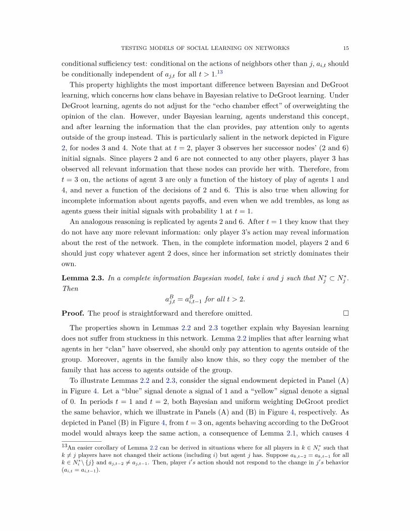
Figure 2. A quilt on 7 nodes, which is network 3 in our experiment.
2.2. Fundamental Properties of Bayesian and DeGroot Action Learning. Wenow explore the relevant features of DeGroot action learning and Bayesian learning in thetopologies we chose for our experiment, in order to understand the divergence of theirpredictions. This helps demonstrating why differences in the learning processes lead tovery different patterns for these networks, which is what we desire in the data in orderto distinguish between the learning models. To fix ideas, we concentrate on topology 3(as shown in Figure 2) in our experiment and contrast uniform DeGroot weighting withcomplete information Bayesian learning.10
We focus on three properties. First, networks that have “clans,” in a sense describedbelow, have agents who get stuck on the wrong action under DeGroot learning but notunder Bayesian learning. Second, under complete information Bayesian learning, an agentwhose neighborhood entirely envelops one of her neighbor’s neighborhood ignores thatneighbor’s action outside of her initial action which reflected her signal. This is not trueunder DeGroot learning. Third, under complete information Bayesian learning, an agentwhose information set is dominated by a neighbor only copies her neighbor’s previousperiod action. Again, this is not true under DeGroot learning.
Let us begin with a benchmark. Notice that, if agents had access to all relevant in-formation available (i.e., everyone could observe all signals), the optimal decision wouldthen be to guess the majority, which would make agents under the Bayesian and the uni-form weighting models to coincide. We later show that, in topology 3, the network shapeprecludes some players to have access to information in other parts of the network underDeGroot learning, but under Bayesian learning they are able to overcome this constraint.
We define a node to be stuck if, from some period on, the actions she chooses are oppositeto the optimal decision with full information (i.e., the actions are different from the majorityof signals). Next, we show that tightly knit groups, which we call clans (groups that havemore links to the group than to outsiders), are prone to getting stuck and cannot get newinformation from outside of the clan under DeGroot learning.
10We focus on uniform DeGroot weighting because this is the DeGroot model that best describes the data,as seen below.

TESTING MODELS OF SOCIAL LEARNING ON NETWORKS 13
Figure 3. Distribution of stuck nodes in topology 3 under Bayesian andDeGroot with uniform weighting.
Given a network G = (V,E) and a subset H ⊂ V , we define G(H) := (V (H), E(H))as the induced subgraph for group H. That is, we only considering edges between agentsin H. We write di(H) as the degree of the induced subgraph of group H. We say that agroup C ⊂ V is a clan if for all i ∈ C we have di(C) > di(V \C) (including herself). Thereare various clans in network 3 from our experiment. Triangles, such as (134) and (236),are clans, as are their unions.
We show that under uniform DeGroot weighting, if at some point a clan chooses thewrong action, an action that is the opposite of what one who observes the majority ofsignals would have selected, then it continues to choose it no matter how the rest of thenetwork behaves.
Lemma 2.1. Assume uniform DeGroot weighting. Take C ⊂ V such that for all i ∈ C,di(C) > di (V \C). Assume there exists some t such that for all i, j ∈ C : a(i, t) = a (j, t).Then a(i, t+ τ) = a for all i ∈ C and τ > 0.
Proof of Lemma 2.1. The proof is by induction. Without loss of generality, supposea (i, t) = 1 for all i ∈ C. Of course, for τ = 0 the result is true. Suppose a (i, t+ τ − 1) =1 for all i ∈ C. Let T u (i, t+ τ) = 1
di+1
[a (i, t+ τ − 1) +
∑j∈Ni
a (j, t+ τ − 1)]be the
index that defines uniform weighting (as in equation 2.1) so that if T u (i, t+ τ) > 1/2then a (i, t+ τ) = 1, independent of the particular tie breaking rule used. We show that

TESTING MODELS OF SOCIAL LEARNING ON NETWORKS 14
T u (i, t+ τ) > 1/2:
T u (i, t+ τ) =∑j∈Ni∪i∩C a (j, t+ τ − 1)
di + 1 +∑j∈Ni∩Cc a (j, t+ τ − 1)
di + 1
=︸︷︷︸(i)
di (C) + 1di + 1 +
∑j∈Ni∩Cc a (j, t+ τ − 1)
di + 1
≥ di (C) + 1di + 1 ,
using in (i) the fact that a (j, t+ τ − 1) = 1 for all j ∈ C. Since di = di (C) + di (V \C) forany set C : i ∈ C, and di (C) > di (V \C), we then have that di(C)+1
di+1 > 1/2, as we wantedto show.
The fact that clans can get stuck under DeGroot learning is a key cause in the divergencebetween Bayesian and uniform DeGroot models in topology 3. Figure 3 shows the prob-ability distribution of the number of stuck nodes under Bayesian and uniform weightingDeGroot; Bayesian learning coincides with full information learning 99% of the time whilethis happens in the DeGroot model 63% of the time.11 We can also check (by inspectionof each particular signal endowment) that each instance for which two or more agents arestuck in uniform weighting DeGroot comes from the implication of Lemma 2.1.
We derive below some properties of Bayesian learning that explain the predictions ofBayesian learning for this network without the need of futrher calculations. These prop-erties are enough to eliminate stuckness across most (99% of) signal endowments in thisexample.
Formally, let N∗i = Ni ∪ i be the neighborhood of agent i (including herself), and letati = (ai,1, ai,2, . . . , ai,t). In general, we have that if agent i is Bayesian, and j ∈ N∗i , then
aBi,t = Function((at−1k
)k∈N∗i
). The following statement is then true.12
Lemma 2.2. Suppose N∗i ⊇ N∗j and that for all ω ∈ Ω, aj,1 (ω) = sj. Then, at t > 2, sjis sufficient for
(atj
)when explaining aBi,t. That is,
aBi,t = Function(sj ,(at−1k
)k∈Ni\j
).
Proof. The proof is straightforward and therefore omitted.
This property follows from the fact that, if player j′s action reveals no new informationj′schoice only then matters through the signal she observed; i.e. sj = aj,1. This implies a
11Note that the Bayesian model predicts that either no one gets stuck or everyone does, since there isconvergence.12This is true for larger type spaces Ω, not just when it represents the signal endowments. This includesthe incomplete information model that we explore below.
TESTING MODELS OF SOCIAL LEARNING ON NETWORKS 15
conditional sufficiency test: conditional on the actions of neighbors other than j, ai,t shouldbe conditionally independent of aj,t for all t > 1.13
This property highlights the most important difference between Bayesian and DeGrootlearning, which concerns how clans behave in Bayesian relative to DeGroot learning. UnderDeGroot learning, agents do not adjust for the “echo chamber effect” of overweighting theopinion of the clan. However, under Bayesian learning, agents understand this concept,and after learning the information that the clan provides, pay attention only to agentsoutside of the group instead. This is particularly salient in the network depicted in Figure2, for nodes 3 and 4. Note that at t = 2, player 3 observes her successor nodes’ (2 and 6)initial signals. Since players 2 and 6 are not connected to any other players, player 3 hasobserved all relevant information that these nodes can provide her with. Therefore, fromt = 3 on, the actions of agent 3 are only a function of the history of play of agents 1 and4, and never a function of the decisions of 2 and 6. This is also true when allowing forincomplete information about agents payoffs, and even when we add trembles, as long asagents guess their initial signals with probability 1 at t = 1.
An analogous reasoning is replicated by agents 2 and 6. After t = 1 they know that theydo not have any more relevant information: only player 3’s action may reveal informationabout the rest of the network. Then, in the complete information model, players 2 and 6should just copy whatever agent 2 does, since her information set strictly dominates theirown.
Lemma 2.3. In a complete information Bayesian model, take i and j such that N∗j ⊂ N∗j .Then
aBj,t = aBi,t−1 for all t > 2.
Proof. The proof is straightforward and therefore omitted.
The properties shown in Lemmas 2.2 and 2.3 together explain why Bayesian learningdoes not suffer from stuckness in this network. Lemma 2.2 implies that after learning whatagents in her “clan” have observed, she should only pay attention to agents outside of thegroup. Moreover, agents in the family also know this, so they copy the member of thefamily that has access to agents outside of the group.
To illustrate Lemmas 2.2 and 2.3, consider the signal endowment depicted in Panel (A)in Figure 4. Let a “blue” signal denote a signal of 1 and a “yellow” signal denote a signalof 0. In periods t = 1 and t = 2, both Bayesian and uniform weighting DeGroot predictthe same behavior, which we illustrate in Panels (A) and (B) in Figure 4, respectively. Asdepicted in Panel (B) in Figure 4, from t = 3 on, agents behaving according to the DeGrootmodel would always keep the same action, a consequence of Lemma 2.1, which causes 413An easier corollary of Lemma 2.2 can be derived in situations where for all players in k ∈ N∗i such thatk 6= j players have not changed their actions (including i) but agent j has. Suppose ak,t−2 = ak,t−1 for allk ∈ N∗i \ j and aj,t−2 6= aj,t−1. Then, player i′s action should not respond to the change in j′s behavior(ai,t = ai,t−1).

TESTING MODELS OF SOCIAL LEARNING ON NETWORKS 16
1
2 3 4 5
6 7(a) Signal endowment and pe-riod t = 1 for both models
1
2 3 4 5
6 7(b) Period t ≥ 2 for DeGrootlearning, and period t = 2 forBayesian learning
1
2 3 4 5
6 7(c) Period t = 3 for Bayesian learning
1
2 3 4 5
6 7(d) Period t ≥ 4 for Bayesian learning
Figure 4
agents to be stuck, choosing the inefficient action. As illustrated in Panel (C) in Figure4, from period t = 3 on, according to Lemma 2.2, agents 1 and 3, behaving as Bayesianagents, only need to learn about the initial signals obtained by agents 5 and 7, observingonly player 4’s decisions. After observing player 4’s decision at t = 2, both 1 and 3 realizethat the only signals consistent with her decision is that both s5 and s7 are equal to s4: ifnot, she would have picked a4,t=2 = blue, as 1 and 3 did. Since at t = 2 all agents chooseaccording to the majority of their neighborhood, only s5 = s7 = s4 has positive probabilitygiven their information. Knowing this, player 3’s belief support is singleton, and knowsthat the full-information decision is a3,t=3 =yellow. Lastly, Panel (D) in Figure 4 showsthat, at t = 4, agent 1 knows 3 knew the full signal endowment when choosing at t = 3,and hence a1,t=4 = yellow. With respect to players 2 and 6, we use Lemma 2.3 to predictthat they copy 3’s action in the previous periods.
2.3. Comparing the Asymptotic Properties of Bayesian and DeGroot Learning.The purpose of this section is to compare how different learning models behave in achievingasymptotic learning in large networks, and thus motivate the relevance of the empiricalexcercise in this paper. We also compare the properties of the DeGroot communication

TESTING MODELS OF SOCIAL LEARNING ON NETWORKS 17
models, and conclude that the main difference between the DeGroot communication modeland action models is the coarseness of the message space in the latter. We show that forsensible sequences of networks, both Bayesian action and DeGroot communication modelslead to asymptotic efficiency (where all but a vanishing share of agents make the rightdecision about the state of the world) wherein DeGroot action models can yield a non-vanishing share of agents that are stuck, which highlights the importance of the empiricalexercise we conduct.
Among others, DeGroot (1974), DeMarzo et al. (2003) and Golub and Jackson (2010)study DeGroot models where agents can pass on a continuous value to their neighborsas compared to a binary action. There are two interpretations of this setting: (a) theinformation is in the form of probabilities about a state of the world or (b) agents areestimating a state distributed with noise on a line. It is useful to interpret the model asthe former case, where agents are endowed with signals that give posterior probabilitiespi = P (θ = 1|si).14 In the DeGroot communication model these can be any number in[0, 1], and thus, in the probability interpretation they imply non-atomic posteriors givensignals. This is equivalent to having a continuum of signals, with distributions P (s | θ = 0)and P (s | θ = 1). Without loss of generality, we can assume si = pi directly.
In Golub and Jackson (2010) agents are able to communicate their estimate of pi =P (θ | si), and aggregate their information by taking averages of the estimations of theirneighbors. This is the crucial distinction between the communication model and the actionmodel, where the former is particularly granular and the latter is considerably coarser. Westudy one of the particular cases they focus on, which is analogous to uniform weightingDeGroot model, where agents can communicate their estimation of the probability thatθ = 1 rather than a binary action, and form their next posterior belief as
(2.4) pi,t = 1di + 1
∑j∈Ni
pj,t−1.
A key objective of Golub and Jackson (2010) is to find the conditions under which asequence of growing networks achieve “wisdom of crowds” asymptotically. Formally, takea sequence of networks Gn = (Vn, En) where |Vn| = n, let p(n)
i,t be defined as in2.4 for theneighborhood Ni (n) ⊂ Vn. They define a sequence of graphs Gn to be wise (in the uniformweighting model) if
(2.5) plimn→∞
maxi∈Vn
∣∣∣∣ limt→∞p
(n)i,t − P (θ = 1)
∣∣∣∣→ 0.
Note that if a sequence of networks is wise, then when choosing ai ∈ 0, 1 as the bestresponse to those beliefs, asymptotically they would take the correct decision, as if all
14This is consistent with the results presented in Golub and Jackson (2010), since they assume that pi ∈[0, 1].

TESTING MODELS OF SOCIAL LEARNING ON NETWORKS 18
information was observed. Formally, we say that a sequence is asymptotically efficient iflimt→∞
∣∣∣ai,t − 1(pi,t >
12
)∣∣∣ = 0.We want to compare the DeGroot communication model (with richer communication
channels than the action model we consider) to the performance of the Bayesian andDeGroot action models we test in our experiments, where the beliefs pi,t are derived fromBayes rule or by making weighted averages of past actions, rather than past beliefs. Tomake this comparison, we need to consider a common environment, so we will assume thatagents observe a continuum of signals, rather than the binary signals of our experiment.We see that under very general conditions, both the DeGroot model of Golub and Jackson(2010) and the Bayesian model achieve asymptotic efficiency, but the uniform weightingDeGroot model may not.
Proposition 2.1. Suppose Gn = (Vn, En) with |Vn| = n is such that (i) di (Vn) ≤ d forall i, n (i.e., they have uniformly bounded degrees), (ii) the posterior distributions P (θ | si)are non-atomic in s, for θ ∈ 0, 1, and (iii) signals are i.i.d across agents . Then
(1) the DeGroot communication model is asymptotically efficient,(2) the Bayesian action model is asymptotically efficient, and(3) the DeGroot action model may not be asymptotically efficient.
In particular, suppose there is a sequence of groups An ⊂ Vn such that An =⋃hnk=1C
nk is a strictly increasing family of disjoint clans with uniformly bounded
size. Then the DeGroot action model is not asymptotically efficient.
Proof. The efficiency of the DeGroot communication model is a consequence of Corollary1 in Golub and Jackson (2010). The result on Bayesian action models is the centralTheorem in Mossel et al. (Forthcoming). The inefficiency of DeGroot action model is asimple corollary of Lemma 2.1, since as hn →∞ and signals are non-atomic and i.i.d., thenalmost surely they will be at least a clan Cnk∗ such that ai,1 6= θ for all i ∈ Cnk∗ .
Is worth noting that the asymptotic efficiency result does not crucially depend on thenon-atomicity of posteriors, but rather on the possibility of ties (when pi,t = 1/2). Innetworks where ties do not occur (or occur with vanishing probabilities) then the asymp-totic efficiency result is also true for the case of binary signals (an implicit result in Mosselet al. (Forthcoming), which is also shown in Menager (2006)). In Appendix C we alsoillustrate the impact of this source of asymptotic inefficiency in a particular growing classof networks, which are growing extensions of network 3 from our experiment.
Golub and Jackson (2010) show that the asymptotic result generalize to a greater set ofweighting formulas, as long as the influence of a single agent on the average of everyone inthe network is arbitrarily small as the network size grows. A similar result of inefficiencywould also be true for the DeGroot action model as well, using a variant of Lemma 2.1.
Proposition 2.1 also illustrates the main discrepancy between these models in terms ofsocial learning and why differentiating between which model is used is relevant. If agents

TESTING MODELS OF SOCIAL LEARNING ON NETWORKS 19
cannot communicate (in a credible manner) all the information they have observed (forexample, can only show what they choose or agents just observe neighbors’ decisions) thenthe coarseness of these messages cause the averages taken to get “stuck” on a particularaction, not allowing the flow of new information. This is prevented in the DeGroot com-munication model by allowing pi,t to take any number in [0, 1], so small changes in beliefsare effectively passed through to other agents. Action models make more sense in situa-tions where agents need verifiable information through costly signals (e.g., the actions theytake) to believe the information to be credible or environments where the state or beliefsare complex to describe and communicate.
2.4. An Example from Indian Village Networks. The above results have shown thatwhether asymptotic efficiency is reached or not depends on the structure of networks inquestion. In this section we explore real-world network data to assess whether the problemof DeGroot action learning is relevant in realistic social network structures.
We consider data from Banerjee et al. (2013) consisting of detailed network data in 75villages in Karnataka, India. We consider the networks consisting of information rela-tionships, which in other work we have shown to correlate strongly with favor exchangerelationships. We show that a DeGroot action learning process is likely to get stuck.
0.1 0.2 0.3 0.4 0.5 0.6 0.7 0.8 0.9 1Fraction failing to learn
0
0.1
0.2
0.3
0.4
0.5
0.6
0.7
0.8
0.9
1
F(x
)
CDF of fraction who fail to learn across 75 Indian Villages
p = 0.525p = 0.55p = 0.575p = 0.6p = 0.66
0 0.1 0.2 0.3 0.4 0.5 0.6 0.7 0.8 0.9 1Fraction failing to learn
0
0.1
0.2
0.3
0.4
0.5
0.6
0.7
0.8
0.9
1
F(x
)
CDF of fraction who fail to learn across Erdos-Renyi Graphs
p = 0.525p = 0.55p = 0.575p = 0.6p = 0.66
(A) (B)
Figure 5. Both panels (A) and (B) present CDFs of the fraction of nodesthat initially received the signal 1 − θ that became stuck at the wrongbelief for various levels of p. Panel (A) presents results where we conductsimulations using the 75 Indian village networks from Banerjee et al. (2013).Panel (B) presents the same results for Erdos-Renyi networks which havean average degree that matches the Indian network data.
In Panel (A) we examine simulations conducted on the 75 empirical networks and quan-tify the degree of stuckness. Specifically, with a signal quality of 0.55, in the median village,at least 78% of the nodes that initially received the wrong information stay stuck at the

TESTING MODELS OF SOCIAL LEARNING ON NETWORKS 20
wrong belief. Even with a signal quality of 0.66, in the median village, at least 37% ofhouseholds that initially received the wrong information stay stuck. Furthermore, in over1/3 of the villages, at least 50% of households that initially received the wrong informationstay stuck. In Panel (B) we repeat the exercise but for Erdos-Renyi graphs calibrated tohave an average degree that matches the empirical data. We find, similarly, that DeGrootaction learning is likely to get stuck. But furthermore, by comparing the simulations underthe Indian village networks and the corresponding Erdos-Renyi graphs, we can see thatthe problem is somewhat exacerbated for the empirical networks. For instance, 90% ofempirical network simulations have at least 35% of nodes failing of to learn whereas thecorresponding number is at least 18% for Erdos-Renyi graphs. This suggests evidence that,as shown in Jackson et al. (2012), the networks organized to aid informal transactions deal-ing with limited commitment have generated structures that are prone to misinformationtraps.
3. Experiment
3.1. Setting. We conducted 95 experimental sessions with the three chosen networksacross 19 villages in Karnataka, India. The experiments had 665 total subjects. Thevillages range from 1.5 to 3.5 hours’ drive from Bangalore. We chose the village setting be-cause social learning through networks is of the utmost importance in rural environments;information about new technologies (Conley and Udry, 2010), microfinance (Banerjee et al.,2013), political candidates (Cruz, 2012; Cruz et al., 2015), among other things, propagatesregularly through social networks.
3.2. Implementation and Game Structure. In every village, we run an average of 5sessions, each with 7 participants, given that each of the networks of our experiment had7 nodes. We recruited an average of 35 individuals from a random set of households fromeach village. We brought the individuals to a public space (e.g., marriage hall, school,dairy, barn, clusters of households) where we conducted the experiment. While individualswere recruited, the public space was divided into “stations.” In each station there was asingle surveyor to monitor the single participant assigned to the station at random. Thisensured that participants could not observe each other nor could they communicate. Oftentimes, stations would be setup across several buildings.
In each village, individuals anonymously played the social learning game three times,each time with a different network structure. The three networks (see Figure 6) were playedwith a random order in each village to avoid order effects. At the beginning of each game,all participants were shown two identical bags, one with five yellow balls and two blueballs and the other, with five blue balls and two yellow balls. One of the two bags waschosen at random to represent the state of the world. Since there was an equal probabilitythat either bag could be chosen, we induced priors of 1/2. As the selected bag contained

TESTING MODELS OF SOCIAL LEARNING ON NETWORKS 21
five balls reflecting the state of the world, participants anticipated receiving independentsignals that were correct with probability 5/7.
After an initial explanation of the experiment and payments, the bag for the first gamewas randomly chosen in front of the participants. The participants were then assigned tostations where each was shown a sheet of paper with the entire network structure of sevenindividuals for that game, as well as her own location in the network. The neighbors’ pastdecisions were also communicated to subjects on sheets of paper that presented an imageof the network and colored in their neighbors’ guesses.
Once in their stations, after receiving their signals in round zero, all participants simulta-neously and independently made their best guesses about the underlying state of the world(i.e., which bag had been selected). The game continued to the next round randomly andon average lasted 6 rounds. If the game continued to the second round, at the beginning ofthis round, each participant was shown the round one guesses of the other participants inher neighborhood through the mentioned procedure. Agents updated their beliefs aboutthe state of the world and then again made their best guesses about it. Once again, thegame continued to the following round randomly. This process repeated until the gamecame to an end. Notice that, after the time zero set of signals, no more signals were drawnduring the course of the game. Participants could only observe the historical decisions oftheir neighbors and update their own beliefs accordingly. Importantly, so that we wouldnot bias individuals’ updating against Bayesian learning individuals kept the informationabout the guesses of their neighbors in all previous rounds until the game concluded. Aftereach game, participants were regrouped, the color of the randomly chosen bag was shown,and if appropriate, a new bag was randomly chosen for the next game. Participants werethen sent back to their stations and the game continued as the previous one. After allthree games were played, individuals were paid Rs. 100 for a randomly chosen round froma randomly chosen game, as well as a Rs. 20 participation fee. Participants then facednon-trivial incentives to submit a guess that reflected their belief about the underlyingstate of the world. The incentive was about three-fourths of a daily agricultural wage.
3.3. Network Choice. We selected networks specifically so that we could separate be-tween various DeGroot and Bayesian models considered in the paper.
The previous experimental literature on Bayesian learning on networks (Choi et al. (2005,2012)) make use of several three-person networks. However, we are unable to borrow thesenetworks for our study as they were not designed for the purpose of separating betweenDeGroot and Bayesian learning. In fact, the networks utilized in Choi et al. (2005, 2012)lack power to pit Bayesian learning against the DeGroot alternatives posited above. PanelA of Table 1 shows the fraction of observations that differ across complete informationBayesian learning and the DeGroot alternatives for each of the three networks used in Choiet al. (2005) and Choi et al. (2012). In two of the networks, there are no differences betweenthe equilibrium paths of Bayesian learning and the uniform and degree weighted DeGroot

TESTING MODELS OF SOCIAL LEARNING ON NETWORKS 22
1
2
3
4
5
6
7(a) Network 1
1
2
3
4 5
6 7(b) Network 2
1
2 3 4 5
6 7(c) Network 3
Figure 6. Network structures chosen for the experiment.
alternatives (with a difference with eigenvector weighting of 6.8% in one of the networks).While in the third network, the differences are on average 15.5% of the observations, theseare largely an artifact of many indifferences along equilibrium path for the DeGroot models,which were broken by choosing the individuals’ past action.
Given our goal of separating between Bayesian and DeGroot alternatives, we move toan environment with seven agents as opposed to three, so that we obtain more powerto distinguish between these models while still maintaining computational tractability.Additionally, we consider a quality signal (p = 5/7) to prevent that the separation fromdifferent learning models is driven by indifferences along equilibrium path, and thus, thetie-breaking rule.15
In order to select our three networks, we initially considered all connected and undi-rected networks with seven nodes. Additionally, to prevent indifferences along equilibriumpath, we restricted to networks where the minimum degree of a given individual is two.Further, to avoid confusing our experimental subjects, we restricted to planar networks(networks that can be drawn so that their edges intersect only at their endpoints). Next,we established a model selection criterion function. This criterion function depended on thepower to detect a DeGroot alternative against a complete information Bayesian null, using15Moving to eight agents, for instance, would be exponentially more difficult for our structural estimation.

TESTING MODELS OF SOCIAL LEARNING ON NETWORKS 23
.6.7
.8.9
1Power
.02 .04 .06 .08 .1 .12Divergence
.6.7
.8.9
1Power
.02 .04 .06 .08 .1Divergence
(A) Network 1 (B) Network 2
Figure 7. (A) depicts the power and divergence frontier for degree weight-ing DeGroot. (B) shows the power and divergence frontier for uniformweighting
our pilot data to generate an estimate of the noise, as well as a divergence function. Thedivergence function measures the share of node-time observations for which the Bayesianmodel (with π = 1) and a DeGroot model pick different actions,
D (G) := 1n (T − 1)
∑s∈S
T∑t=2
n∑i=1
∣∣∣aBi,t (s | G)− ami,t (s | G)∣∣∣ · P (s | θ = 1) ,
where aBi,t(s | G) is the action predicted under the Bayesian model and ami,t(s | G) isthe action predicted under DeGroot with m-weighting, where m is uniform, degree, oreigenvector weighting.16
Figure 7(A) depicts a scatter plot of power and divergence for network 1 in Figure 6.We see that our network 1 is the best ex-ante choice to separate between the incompleteinformation Bayesian and DeGroot degree weighting models. Figure 7(B) illustrates theanalogous figure for network 2 in Figure 6, and highlights that it is the best ex-ante choiceto separate between the Bayesian and DeGroot uniform weighting models. Lastly, thechoice of network 3 in Figure 6 was motivated by our exercise in section 2, and by thefact that it performed very well in separating between the Bayesian and both the DeGrootuniform and degree weighting models.
4. Testing the Theory
4.1. Estimation and Inference. In order to test how well model m fits the data insession r, we use the fraction of discrepancies between the actions taken by individuals in
16P (s | θ = 1) = p
∑i
si (1− p)n−∑
isi .

TESTING MODELS OF SOCIAL LEARNING ON NETWORKS 24
the data and those predicted by the model. This is given by
D (m, r;π) := 1n(Tr − 1)
n∑i=1
Tr∑t=2
Dmi,t,r
where Dmi,t,r = |aobsi,t,r − ami,t,r| which computes the share of actions taken by players that are
not predicted by the model m.17 To examine how poorly model m predicts behavior overthe entirety of the data set, we define the divergence function as
D (m;π) := 1R
R∑r=1
1(Tr − 1)n
n∑i=1
Tr∑t=2
Dmi,t,r.
This is simply the average discrepancy taken over all sessions. Model selection is based onthe minimization of this divergence measure. Note that we include dependency on π, theshare of Bayesian agents believed to be in the population, since for the Bayesian model,the prediction ami,t,r depends on π. The computation of the Bayesian actions are describedin Appendix A.
While the divergence is the deviation of the observed data from the theory, we may definethe action prescribed by theory in one of two ways. First, we may look at the network level,which considers the entire social learning process as the unit of observation; and second,we may study the individual level wherein the unit of observation is an individual’s actionat an information set.
When studying network level divergence, we consider the entire learning process as asingle observation. Theory predicts a path of actions under the true model for each indi-vidual in each period given a network and a set of initial signals. This equilibrium paththat model m predicts is given the theoretical action ami,t,v. When using this approach,we try to assess how the social learning process as a whole is explained by a model. Thismethod maintains that the predicted action under m is not path-dependent and is fullydetermined by the network structure and the set of initial signals.
When we consider the individual level divergence, the observational unit is the individual.The action prescribed by theory is conditional on the information set available to i at t−1and the ex-ante probability that a given individual is a Bayesian learner as opposed tosome DeGroot-alternative learner: ami,t,v is the action predicted for agent i at time t insession r, given information set Pi,r,t and π.
For every DeGroot alternative, we consider the probability that minimizes the divergencefunction:
πm = argminπ∈[0,1]
D (m;π)
where m indexes an incomplete information Bayesian model with each of the possibleDeGroot alternatives: uniform, degree, and eigenvector. In order to perform inference on
17Since all models and all empirical data have a fixed first action (given by the signal endowment), the firstround should not enter into a divergence metric. Thus, we restrict attention to t ≥ 2.

TESTING MODELS OF SOCIAL LEARNING ON NETWORKS 25
the parameter, we perform a block Bayesian bootstrap that accounts for the dependence inthe data of the individuals playing the same game (see a similar procedure used in Banerjeeet al. (2013)).
Equipped with the minimizing value of πm for m ∈ u, d, e, we are prepared to conductour analysis. Note that procedure is done both at the network level and the individuallevel. In particular, in addition to simply identifying the best-fitting model, we can go onestep further and ask whether incorrect beliefs about others’ types can explain the data.Specifically, given πm, we can ask whether the divergence can be minimized further by,for instance, drawing a population of all Bayesian agents who have heterogeneous priorsand lack common knowledge of Bayesian rationality, and therefore are employing πm as amistaken belief. We are able to assess whether deviations from correct beliefs can rationalizethe data better than a singular DeGroot alternative. Finally, we can also look at a non-nested hypothesis test of how the model with common knowledge of Bayesian rationalitycompares to each of the DeGroot alternatives, and how the DeGroot models compare toeach other in terms of explaining the data.
4.2. Learning at the Network Level. We begin by treating the social network and theentire path of actions as a single observation.
4.2.1. Comparing DeGroot and Complete Information Common Knowledge Bayesian Mod-els. Before looking at the incomplete information estimation result, we begin by first look-ing at comparisons of the three DeGroot models and the common knowledge, completeinformation Bayesian model. Figure 8 presents the data in a graphical manner and Table2 presents the results for non-nested hypothesis tests comparing each of the models in apairwise manner.
0
0.05
0.1
0.15
0.2
0.25
All Network 1 Network 2 Network 3
Bayesian
Uniform
Degree
Eigenvector
Figure 8. Fraction of actions unexplained at the network level

TESTING MODELS OF SOCIAL LEARNING ON NETWORKS 26
As seen in Figure 8, across all the networks, uniform weighting fails to explain 12% of thedata, degree weighting fails to explain 14% of the data, eigenvector-centrality weightingfails to explain 13.5% of the data, and complete information Bayesian learning fails toexplain 18% of the data. This suggests that the DeGroot models, as well as the Bayesianlearning models each explain more than 80% of the observations, but the DeGroot modelsdo considerably better.
Turning to the pairwise comparisons of fit, we conduct a non-nested hypothesis test(Rivers and Vuong, 2002) using a nonparametric bootstrap at the session-game level,wherein we draw, with replacement, 95 session-game blocks of observations and computethe network level divergence.18 This procedure is analogous to clustering and, therefore, isconservative exploiting only variation at the block level. We then create the appropriatetest statistic, which is a normalized difference of the divergence functions from the twocompeting models.
Our key hypothesis of interest is a one-sided test with the null of Bayesian learningagainst the alternative of the DeGroot model. Table 2 presents the p-value results of theinference procedure. Note that most of the values are essentially zero. First, lookingacross all topologies both separately and jointly, we find evidence to reject the Bayesianmodel in favor of all the DeGroot alternatives. Second, we find that uniform weightingdominates every alternative across every topology both separately and jointly. Ultimately,the bootstrap provides strong evidence that the uniform-weighting DeGroot model bestdescribes the data generating process when analyzed at the network level.
4.2.2. Incomplete Information Bayesian Learning. We now present our main results usingthe network level divergence. The estimation algorithm is described in Appendix A. PanelA in Table 3 displays the minimizing parameter estimate π for in incomplete informationBayesian learning model with each of the DeGroot alternatives. We robustly find thatthe minimizing parameter value is πm = 0 for every model m. This suggests that, if thecommon knowledge parameter π truly describes the population distribution, essentially0% of the population is Bayesian and any Bayesian agent believes 0% of the population isBayesian. Doing a session level bootstrap, we estimate the standard errors as 0.08, 0.12and 0.09 respectively across uniform, degree and eigenvector alternatives. This shows thatdespite the uncertainty, at best only a very small share of agents could likely be Bayesian.
Our results then indicate that when we estimate a model of incomplete informationlearning with potentially Bayesian agents, the model that best describes the data is onethat is equivalent to having no Bayesians whatsoever and instead describing each agent asDeGroot. Moreover, the results of Table 2 indicate that that the best fitting such modelis one with uniform weighting.
18We have 95 village-game blocks in networks 1 and 2, and 75 for network 3. We redraw with replacementthe same number that we have in our empirical data.

TESTING MODELS OF SOCIAL LEARNING ON NETWORKS 27
To give the Bayesian social learning model another shot at better describing the exper-imental data, we conduct a second exercise. We consider the case where all agents areBayesian, but we relax the common prior assumption. Specifically, we allow for each agentto be Bayesian, know that she is Bayesian, but be uncertain about whether others areBayesian or not. So each agent believes that a π share of the population is non-Bayesian,despite the fact that everyone is indeed Bayesian. We then compute the divergence min-imizing π for a model where all agents are Bayesian but there is no common knowledgeof Bayesian rationality but instead is a miscentered belief on the distribution of Bayesiantypes via heterogenous priors. Here we find the best fitting parameters across all networksto be π = 0 for every model m (Panel C of Table 3). Unsurprisingly, however, the stan-dard errors are larger in this case. By looking at the divergence at the optimal π, we cansee that drawing individuals from the distribution given by πm fits the data considerablybetter than assuming all agents are Bayesian but incorrectly believing that others couldbe DeGroot types (see Panels B versus D).
To summarize, as illustrated by Figure 9, whether considering common knowledge ofBayesian rationality or not, the robust best explanation of the data is the simplest modelwith π = 0. Here every agent is DeGroot.
4.3. Learning at the Individual Level. Having looked at the network level divergence,we turn our attention to individual level divergence. While this does not purely address themechanics of the social learning process as a whole, it does allow us to look at individuallearning patterns. Understanding the mechanics of the individual behavior may help usmicrofound the social learning process.19
4.3.1. Complete Information Bayesian Learning. We begin by calculating the individuallevel divergence for the DeGroot models and the model where all agents are Bayesian andcommonly know all are Bayesian.20 This is depicted in Figure 10.
First, uniform weighting systematically outperforms degree weighting (0.0648 versus0.1029), and degree weighting outperforms eigenvector weighting by a small margin (0.1029versus 0.1097). Second, it is worth noting how well the DeGroot models perform in termsof predicted individual behavior. Across all three networks, the uniform weighting modelexplains approximately 94% of all individual observations. Degree and eigenvector cen-trality weighting models predict 90% and 89% of all individual observations, respectively.Finally, the common knowledge of Bayesian rationality model performs rather poorly, pre-dicting 74% of all individual observations, and consequently, significantly underperforms
19It is certainly ex-ante possible that agents themselves do not each behave according to a particular modelwhile the aggregate social group may best be described by such a model.20When an agent faces a tie, they stay with their previous action. We considered a random tie-breakingalternative as well, which does not substantively change the results. Importantly, as explained below, Figure10restricts to the observations in the support with positive probability under the complete informationBayesian learning model.

TESTING MODELS OF SOCIAL LEARNING ON NETWORKS 28
π π(A) Uniform weighting (B) Degree weighting
π(C) Eigenvector weighting
Figure 9. Fraction of actions unexplained by incomplete informationmodel at various π. We show expected divergences (where we plot the shareof actions unexplained under π share Bayesian agents where each agent isdrawn Bayesian with probability π and DeGroot with probability 1−π). Wealso show divergences when all agents are Bayesians but mistakenly thinkthat other agents could be DeGroot with probability 1− π.
at explaining the data relative to all-DeGroot models. Accordingly, Table 4 provides thehypothesis tests for the non-nested model selection procedure to show that the completeinformation Bayesian-learning model can be rejected in favor of DeGroot-learning alterna-tives.
We also provide a non-parametric test using just network 3 in our sample. Notice thatin this network peripheral nodes that behave according to the Bayesian-learning modelshould follow the action of its parent node in the graph in any period t > 3. This isbecause the peripheral nodes’ information sets are dominated by those of the parent node.Table 5 shows that only 17% of the time when the Bayesian and DeGroot models predictcontradicting guesses do the agents actually take the Bayesian decision. This means that

TESTING MODELS OF SOCIAL LEARNING ON NETWORKS 29
Figure 10. Fraction of actions unexplained at the individual level
around 83% of the time, agents are ignoring information dominance and going with a(weighted) majority of their neighborhood.
4.3.2. Zero Probability Information Sets. When considering individual Bayesian learning,observe that there is a possibility that, empirically, Bayesian agents may arrive to aninformation set that has zero probability of occurrence. This is not a conceptual problemwhen we study the network-level divergence, because any deviation from the empirical data,irrespective of the history, is penalized. However, this is problematic for identification whenwe look at the individual level divergence, since the Bayesian learning model is mute whenagents have to condition their inference on zero probability events; any observed actionfrom then on would be admissible for a Bayesian learning agent.
The degree to which this is a problem is highlighted in Table 6. We show the share ofindividuals, the share of sessions, and the share of observations (a given individual in agiven round in a given game) that encounter zero probability information sets. In Panel A,we look at the zero probability information sets reached under the complete informationcommon knowledge model of Bayesian learning. We find that about 45% of individuals,70% of sessions and 40% of observations hit zero probability information sets. In Panels B,C, and D we observe that these numbers modestly decline when we allow for incompleteinformation about others’ types. While this certainly does not eliminate the problem, itdoes provide immediate evidence of the potential value of allowing our Bayesian agents todoubt the Bayes-rationality of her peers.
One natural way to eliminate the zero probability information set problem entirely is tointroduce disturbances. In section 4.3.4, we explore the possibility of estimating a tremblinghand or quantal response equilibrium (QRE) style version of Bayesian learning in which weintroduce the possibility of making mistakes by all agents a la Choi et al. (2012). In such a

TESTING MODELS OF SOCIAL LEARNING ON NETWORKS 30
model, individuals can make mistakes with some probability, and Bayesian agents, knowingthe distribution of these disturbances, integrate over this possibility when updating. Weshow that this approach is computationally infeasible in our context in Proposition 4.2.
Since guaranteeing full support in this model by introducing trembles creates computa-tional problems that we describe below, let us start by discussing what we make of the zeroprobability events we encounter. First, we argue that the fact that we repeatedly observeagents facing zero probability events – even when there is positive probability that agentsmay be behaving in another manner – may be taken as prima facie evidence supportingthe idea that this model of Bayesian learning with incomplete information on networksfails to explain the experimental data. Second, one could make the objection that theconsidered incomplete information Bayesian model, is not sufficiently rich to capture thecharacteristics of the data and that, perhaps, one needs a more nuanced model. This couldindeed be the case, but as demonstrated in Proposition 4.2, it would be computationallyinfeasible to estimate a model generating full support. Third, it might be the case thatwe have the right incomplete information Bayesian model, but we lack a theory of whatindividuals do once they hit zero probability events. If this is the case we may take twodifferent approaches: we could be agnostic about the correct off equilibrium beliefs, or wecould consider the case of a richer Bayesian model that rationalizes the actions taken afteran agent hits a zero probability event and precisely matches the supposed off equilibriumbehavior. Such a model, of course, has the degree-of-freedom problem.
Instead, we take what we believe to be an reasonable approach by considering twoalternatives. In the first case, we penalize each zero probability observation as an error. Inthe second case, we only look at observations in the support of observations with positiveprobability of occurrence under the Bayesian learning model (meaning we do not penalizethe Bayesian model for arriving at zero probability information sets). We report resultsfor both to paint a complete picture.
4.3.3. Incomplete Information Bayesian Learning. We now turn to studying which incom-plete information Bayesian learning model best fits the data, taking these constraints intoaccount. We look at the deviation of each agent’s action, given the history that the agenthas observed at that time, from the predicted action by the model for that agent given thehistory. The formalities are developed in Appendix A.
Table 7 presents the results for the case where we use all rounds of data. We find thatπu = πd = πe = 0. Further, the standard errors are quite small: 0.014, 0.024, and 0.011,respectively for uniform, degree and eigenvector weighting. In addition, in Panel B, we seethat at the optimum (as noted in Figure 10) the divergences are small.
In Table 8, we show results where we constrain ourselves to the support of observationswith positive probability of occurrence under the Bayesian learning model. Here we losea tremendous amount of information. In Panel B, we see that the fraction of observa-tions unexplained rises steeply (almost three-fold) relative to the case where we use all

TESTING MODELS OF SOCIAL LEARNING ON NETWORKS 31
observations. This means that the DeGroot model is explaining behavior precisely whenthe Bayesian model, even with incomplete information, runs into a zero probability infor-mation set. Nonetheless, we find that the divergence minimizing π to πu = πd = 0 andπe = 0.9. Unsurprisingly, the standard errors are considerably larger in this case (0.32,0.28, and 0.31, respectively) and the bootstrapped confidence intervals practically coverthe entire interval. In sum, if we take the view that we must remain agnostic about thezero probability information set observations, then we do not have enough information atthe individual level to distinguish the model for any π.
Finally, as before, we explore what happens if we consider the Bayesian setting but re-move common knowledge of Bayesian rationality. In this case, while the objective functionminimizing parameter estimates are typically far from 0, the divergences are significantlyhigher from those in the incomplete information case with common knowledge of distribu-tion of types.
In summary, we have shown that, when we consider the data at the individual level,because even the incomplete information Bayesian model reaches zero probability informa-tion sets so frequently, when we consider the data inclusive of all observations, the bestexplanation is a simple model where all agents are DeGroot. At the same time, the shareof data unexplained rises steeply when we restrict attention to only observations wherewe have not encountered a zero probability information set. This suggests that the DeG-root model precisely explains the data where the Bayesian models are failing. However,if we take the extreme view to not penalize the Bayesian model at all on zero probabilityinformation sets, then, when conditioning on the history, we do not have the power todistinguish between any model of individual learning with any π.
4.3.4. Bayesian Learning with Disturbances and Complexity Problems. Now we discussexpanding the support by introducing disturbances. For expositional simplicity, we re-strict attention to the case of a complete information Bayesian model where each agent isBayesian. In this environment, each agent makes a mistake with probability ε and choosesthe opposite action that a Bayesian agent would choose. This guarantees full support: anyagent can take any action given any history with positive probability.21
Introducing disturbances comes at great computational cost in an environment whereagents learn on networks. The only sufficient statistic for the information set that eachagent sees is the information set itself, as there is no deterministic function between signalendowments and information sets. This means that through time, the relevant state space(the histories that each agent could have seen) grows exponentially. We show that thismakes the problem intractable for any practical purpose.
21Haile et al. (2008) show that QRE imposes no falsifiable restrictions and can rationalize any distributionof behavior in normal form games. Relating this intuition to our context, one may be able to pick adistribution of ε such that it rationalizes the incomplete information Bayesian model as describing the datawell.

TESTING MODELS OF SOCIAL LEARNING ON NETWORKS 32
First, we note that the algorithm that we use to simulate the Bayesian learning modelwithout trembles is computationally “tight” in the sense that, asymptotically in the numberof rounds, there is no faster algorithm.22 Because any algorithm would have to take order Tsteps to print output for each of the T periods, an algorithm that is O(T ) is asymptoticallytight.
Proposition 4.1. The algorithm for computing Bayesian learning with no disturbances isΘ(T ).23 Moreover, it is asymptotically tight; i.e., any algorithm implementing Bayesianlearning must have running time of at least Θ (T ).
Proof. See the computation in Appendix A.5.
Specifically, the algorithm is Θ(n4nT ). Notice that if n was growing this algorithmwould be exponential time, but here, n is a constant. Second, we show that the extensionof this algorithm to an environment with disturbances is computationally intractable.
Proposition 4.2. Implementing the Bayesian learning algorithm with disturbances hascomputational time complexity of Θ(4n(T−1)).
Proof. See the computation in Appendix A.5.
In order to illustrate the complexity of these algorithms with trembles, we compare themto their deterministic counterparts. For the complete information model, the algorithmwith trembles with T = 6 involves 1.19 × 10¹⁶ more computations than the deterministicmodel. With the same T , the incomplete information model involves 8.65× 1032 more cal-culations than its deterministic counterpart. To see how severe the burden is, suppose thatthe deterministic complete information model takes 1 second to run. Then the determinis-tic incomplete information model (again, without trembles) takes 4 and a half hours. Thetrembling hand complete information model, however, takes approximately 377,346,524years.
Note that the above exercise looked at the number of computations for a specific algo-rithm – one that was efficient for the case without disturbances. An objection could bemade that there may be, perhaps, a more efficient algorithm. In Appendix A.5, we discussthe relationship between our current problem and work on computational complexity inBayesian networks, which gives the reader intuition as to why we believe it is likely impos-sible, if not in the least very difficult, to derive efficient algorithms with trembles in thiscontext.
22Our environment consists of finite graphs where n does not grow in T .23Recall that we say f1(n) ∈ Θ(f2(n)) if f1 is asymptotically bounded above and below by f2, up to amultiplicative constant. Formally, if ∃c1, c2 > 0, n such that ∀n > n, c1 · |f2(n)| < |f1(n)| < c2 · |f2(n)|.

TESTING MODELS OF SOCIAL LEARNING ON NETWORKS 33
4.4. Summary. To summarize this section’s results, first we have presented evidence thatthe considered model of Bayesian learning result often arrives at zero probability informa-tion sets. This can be taken as evidence against these particular models. By relaxing themodel to incomplete information, we can recover some, but not all, of these events. Second,we provide an argument to show that models with trembles, which would smooth out thezero probability information set problem, are of little practical use to structurally evaluateempirical data. In turn, methodologically, structural approaches must restrict themselvesto models which allow for zero probability information sets. Third, we take a pass at thedata by ignoring the off-equilibrium information sets. We lose considerable informationin this case. If we penalize the Bayesian model for zero probability events, the result isparticularly strong with robust estimates suggesting π = 0 irrespective of the DeGrootalternative. Finally, we show that one cannot better fit the data by adding heterogeneouspriors where all agents are Bayesian but each incorrectly believes that each other may beDeGroot with probability π. The results robustly support the results we also found in thenetwork level analysis: DeGroot models with simple weighting (such as uniform weighting)provide a good explanation of the data against a large class of alternatives and informationstructures, though in this case, eigenvector weighting does nearly as well.
5. Why a Lab Experiment with Structural Estimation
In this section, we discuss two reduced form approaches to study the experimental data.The motivation is the following. Given the computational limits of the structural approach,we are interested in seeing whether reduced form patterns of Bayesian learning (as opposedto DeGroot learning) may be obtained from the data. Since larger networks, such asthose found in empirical data sets, do not lend themselves to structural approaches forcomputational reasons, it is worth looking into the effectiveness of reduced form approachesto address these questions.
The central intuition on which we focus concerns double counting information and wasinspired by the work of Möbius et al. (2015). Under any of the aforementioned Bayesianmodels, Bayesian agents should not double-count information. DeGroot agents do double-count information, however, and it is on this intuition that we build the exercise. The workof Möbius et al. (2015) explores an idea like this to look for tagged information, which isdifferent from the question of Bayesian versus DeGroot learning. In our setting, tags areshut down.
We provide two examples of regressions that researchers may run. The first set ofregressions explores whether individuals overweight the same information if they receiveit through multiple channels. The second set of regressions explores whether individualstreat old information that cycles back to them as if it is new, additional information.The naive null in these regressions is Bayesian model, since one would assume that therelevant parameters ought to be zero. Thus, a rejection of a zero may provide evidence

TESTING MODELS OF SOCIAL LEARNING ON NETWORKS 34
in the direction of the DeGroot rules of thumb. The empirical data shows that both ofthese reduced form analyses seem to provide support in favor of the DeGroot alternatives.However, because we are able to simulate out the data under the null, we show that theseintuitions are wrong. Specifically, when we simulate social learning data under the Bayesiannull, the coefficients are not as one may have expected. We can also show, available uponrequest, that we can generate DeGroot-like reduced form parameters for a number ofnetwork topologies under true Bayesian learning, and vice versa.
5.1. Multiplicity. We define a variable which is a dummy for whether individual imakes aguess of 1 in the final period T , yi := 1 ai,T = 1. As before, di is the degree of individuali, and Ni is the set of (direct) neighbors Ni = j ∈ V : ij ∈ E. Note that di = |Ni| .Moreover, let N2i be the set of second-neighbors of person i; that is, j ∈ N2i means thatthere is at least one path of length two between i and j, but no path of length one. Finally,we define N l
2i to be the set of second neighbors to whom she has exactly l paths.The first regression we run is of the form
(5.1) yi = β0 + β1si + β2ENi [sj |j ∈ Ni] +∑l
β3lEN l2i
[sj |j ∈ N l2i] + εi.
This is a regression of whether or not individual i ultimately makes a guess of 1 on whetherthe individual’s signal is 1 (si) the share of ones (ENi [sj |j ∈ Ni]) in individual i’s neigh-borhood, and the share of ones given to each subset of second neighbors to whom i hasexactly l paths (EN l
2i[sj |j ∈ N l
2i]).The interpretation is as follows. β2 measures the impact of her neighborhood receiving a
greater share of ones on an individual’s guess. We expect β2 > 0. Moreover, β3l measuresthe impact of the subset of her second-neighborhood with multiplicity l. The intuition isthat as the signals of individuals with greater multiplicity ought not be double-countedunder a Bayesian frame, β3l+1 > β3l would be evidence of overweighting redundant infor-mation that has arrived via multiple channels, while β3l+1 = β3l would provide evidence infavor of the Bayesian hypothesis.
Given the learning model, the network structure, and signal endowment, we simulatedout the learning path and then ran the relevant regressions. We present results whensimulating the learning process from the complete information Bayesian model (every agentis Bayesian) as well as the two most intuitive DeGroot alternatives.
Table 9 provides the simulation and empirical results. When looking at the empiricalresults, we see that, as expected, an individual’s own signal being one and the shareof individuals in one’s neighborhood with signals of one increase the probability of thefinal guess being one. However, we can reject that β3l+1 > β3l. While this seems tobe inconsistent with the intuition that agents engage in double-counting, the simulationexercise shows that these patterns cannot necessarily be interpreted in that manner. First,columns (3) and (4) indicate that the Bayesian null does not have coefficients that are

TESTING MODELS OF SOCIAL LEARNING ON NETWORKS 35
near identical across multiplicities 1 and 2. Moreover, columns (5) and (6) show that whenwe look at DeGroot learning with degree weighting, it is not the case that β3,2 > β3,1.More generally, the increasing correlation with indirect friends of higher multiplicities isalso not uniformly found across the DeGroot models. Ultimately, the regressions suggestthat the linear projection of this learning process is complex and may depend cruciallyon the network structure, set of initial signals, and the particular communication channelsinvolved.
5.2. Historical Information. Another reduced form analysis that one may conduct isaddressing whether individuals re-incorporate historical information that they have pre-viously observed. Consider an individual at period 3. They have observed both theirown signals and the signals of their direct neighbors (insofar as the first period guesses oftheir neighbors will be identical to their signals). In period three, therefore, a Bayesianindividual’s guess should not re-incorporate this information. Instead, it should only up-date using information about second-neighbors and the like, about whom they have yet toreceive information.
To examine this formally, we perform the following regression. We regress the periodthree guess of individual i on her own signal (si) and the average signal of her neighborhood(ENi [sj |j ∈ Ni]) which she would have seen in period three. We also include as regressorsthe average signal of second neighbors (EN2i [sk|k ∈ N2i]) which should be new informationin period three. Lastly, we include the average signal of direct neighbors whose signalscan cycle back via a path of length two back to individual i. Of course, we also includethe agent herself in this set. Formally, we use ECi [sj |j ∈ Ci], where Ci = j ∈ V − i :A2ijAij > 0 ∪ i . The regression is as follows.
yi = α0 + α1si + α2ENi [sj ] + α3EN2i [sk|k ∈ N2i] + α4ECi [sj |j ∈ Ci] + εi.(5.2)
We test the hypothesis of whether α4 = 0, which is our naive Bayesian null. Notice thatα4 > 0 provides evidence that individuals reincorporate information that they alreadyknew as it cycles through the network.
Table 10 presents the simulation and empirical results. When looking at the empiricalresults, we see that as expected, an individual’s own signal being one and the share ofdirect and new indirect neighbors with signals of one increase the probability of the finalguess being one. Also, the empirical results show that the share of repeated indirectneighbors with signals of one increase the probability of the final guess being one, that is,α4 > 0 . While this seems to provide suggestive evidence for the intuition that DeGrootweighting reincorporates old information, the simulation results provide evidence that forour environment, α4 > 0, even for the Bayesian model.
5.3. Reflection on Reduced Forms. Taken together, Tables 9 and 10 have shown thatnatural reduced form approaches to test between these models may be misguided without
TESTING MODELS OF SOCIAL LEARNING ON NETWORKS 36
first checking whether the patterns by the learning processes actually match the intuitions.We are able to study the reduced form projections of the Bayesian model using our simula-tion algorithm and find evidence that, when projected onto a regression for these networkswith this environment, the Bayesian data suggests that the coefficients can deviate greatlyfrom our intuitions. This, we argue, provides a strong motivation for the structural ap-proach to studying the models.
6. Conclusions
In this paper, we have investigated whether social learning patterns on small networksare better fit by models where individuals construct beliefs in a Bayesian manner or bymodels where individuals are myopic and instead follow DeGroot rules of thumb to computebeliefs. To do so, we developed a simple experiment where we designed networks in orderto distinguish between these models, large enough to give us power on this dimension,but small enough to ensure that simulating a Bayesian learning on networks model wasnot computationally intractable. Given the experimental data, we were able to study thesocial learning process as a whole by taking the network as the unit of observation andstudying the behavior of an individual, which addresses whether an agent acts in a Bayesianmanner. Furthermore, we are able to relax both common knowledge of Bayesian rationality,by allowing agents to be either Bayesian or DeGroot in their learning, modeled as agentshaving privately observed (epistemic) types (as in Harsanyi (1967)). Additionally, we relaxthe common prior assumptions, allowing all agents to be Bayesian (and therefore know it)yet remain unsure as to whether others are Bayesian or DeGroot.
At the network level, we find evidence that the uniform weighting DeGroot model bestexplains the data. The Bayesian learning null is rejected in favor of this alternative model.However, we maintain that Bayesian learning did an adequate job of describing the exper-imental data, largely owing to the fact that in many circumstances, the Bayesian prescrip-tion did not differ from the DeGroot prescription.
At the individual level, we find that uniform weighting DeGroot performs the best, out-performing the Bayesian model. However, we show that the Bayesian model encountersthe problem that many individuals come across zero probability information set. First,this provides suggestive evidence of the lack of fit of this incomplete information Bayesianmodel. Second, we demonstrate that introducing disturbances to smooth out the distri-bution cannot be a solution in this environment. The computational complexity of theproblem is damaging to the very approach of applying QRE or trembles to the Bayesianlearning on networks environment. As such, we recommend that researchers focus oncomputationally tractable models, which will be easier to falsify.
We also show that reduced form approaches may be problematic. We provide two naturalexamples of regressions which build on intuitions separating DeGroot and Bayesian learningpatterns. Equipped with our Bayesian learning algorithm, we simulate learning data from

TESTING MODELS OF SOCIAL LEARNING ON NETWORKS 37
the Bayesian model, as well as from DeGroot models and show that the reduced formregression outcomes do not conform to the intuitions.
Ultimately, the findings suggest that agents and the learning process is rather consistentwith DeGroot action models where individuals myopically weight their neighbors’ actionswhen updating their own beliefs rather from a Bayesian model. This may imply that sociallearning processes, in contexts where agents observe each others’ actions, empirically maybe sub-optimal, with information often getting stuck in pockets of the network. Havingconstructed an example of a network which satisfies asymptotic learning for DeGroot com-munication models, but where asymptotic learning fails for DeGroot action models, weargue that in action-learning environments DeGroot processes may be more damaging tothe wisdom of society than previously anticipated.
References
Acemoglu, D., M. A. Dahleh, I. Lobel, and A. Ozdaglar (2011): “Bayesian Learn-ing in Social Networks,” Review of Economic Studies, 78, 1201–1236.
Anderson, L. and C. Holt (1997): “Information cascades in the laboratory,” TheAmerican Economic Review, 87, 847–862.
Aumann, R. J. (1976): “Agreeing to Disagree,” The Annals of Statistics, 4, 1236–1239.Banerjee, A. (1992): “A simple model of herd behavior,” The Quarterly Journal ofEconomics, 797–817.
Banerjee, A., A. G. Chandrasekhar, E. Duflo, and M. Jackson (2013): “TheDifussion of Microfinance,” Science, 341, 1236498.
Bikhchandani, S., D. Hirshleifer, and I. Welch (1992): “A Theory of Fads, Fashion,Custom and Cultural Change as Information Cascades,” Journal of Political Economy,100, 992–1026.
Brandts, J., A. Ebru Giritligil, and R. A. Weber (2015): “An Experimental Studyof Persuasion Bias and Social Influence in Networks,” European Economic Review, 80,214–229.
Celen, B., S. Kariv, and A. Schotter (2010): “An Experimental Test of Advice andSocial Learning,” Management Science, 56, 1–15.
Choi, S. (2012): “A Cognitive Hierarchy Model of Learning in Networks,” Review ofEconomic Design, 16, 215–250.
Choi, S., D. Gale, and S. Kariv (2005): “Behavioral aspects of learning in socialnetworks: An experimental study,” Advances in Applied Microeconomics: A ResearchAnnual, 13, 25–61.
——— (2012): “Social Learning in Networks: A Quantal Response Equilibrium Analysisof Experimental Data,” Review of Economic Design, 16, 93–118.
Choi, S., E. Gallo, and S. Kariv (2015): “Networks in the laboratory,” WP, March.

TESTING MODELS OF SOCIAL LEARNING ON NETWORKS 38
Conley, T. and C. Udry (2010): “Learning about a new technology: Pineapple inGhana,” The American Economic Review, 100, 35–69.
Corazzini, L., F. Pavesi, B. Petrovich, and L. Stanca (2012): “Influential listeners:An experiment on persuasion bias in social networks,” European Economic Review, 56,1276–1288.
Cruz, C. (2012): “Social Networks and the Targeting of Illegal Electoral Strategies,” .Cruz, C., J. Labonne, and P. Querubin (2015): “Politician Family Networks andElectoral Outcomes: Evidence from the Philippines,” .
DeGroot, M. (1974): “Reaching a consensus,” Journal of the American Statistical Asso-ciation, 69, 118–121.
DeMarzo, P., D. Vayanos, and J. Zwiebel (2003): “Persuasion Bias, Social Influence,and Unidimensional Opinions*,” Quarterly journal of economics, 118, 909–968.
Ellison, G. and D. Fudenberg (1993): “Rules of thumb for social learning,” Journalof Political Economy, 101, 612–643.
——— (1995): “Word-of-mouth communication and social learning,” The Quarterly Jour-nal of Economics, 93–125.
Eyster, E. and M. Rabin (2010): “Naive Herding in Rich-Information Settings,” Amer-ican Economic Journal: Microeconomics, 2, 221–243.
——— (2014): “Extensive Imitation is Irrational and Harmful,” The Quarterly Journal ofEconomics, 129, 1861–1898.
Gale, D. and S. Kariv (2003): “Bayesian learning in social networks,” Games andEconomic Behavior, 45, 329–346.
Geanakoplos, J. (1994): “Common Knowledge. chapter 40 of volume 2 of the Handbookof Game Theory, edited by R. Aumann and S. Hart,” .
Geanakoplos, J. and H. Polemarchakis (1982): “We can’t disagree forever,” Journalof Economic Theory, 28, 192–200.
Golub, B. and M. Jackson (2010): “Naive Learning in Social Networks and the Wisdomof Crowds,” American Economic Journal: Microeconomics, 2, 112–149.
——— (2012): “How homophily affects learning and diffusion in networks,” QuarterlyJournal of Economics, 127, 1287–1338.
Haile, P., A. Hortaçsu, and G. Kosenok (2008): “On the empirical content of quantalresponse equilibrium,” The American Economic Review, 98, 180–200.
Harsanyi, J. C. (1967): “Games with Incomplete Information Played by "Bayesian"Players, I-III. Part I. The Basic Model,” Management Science, 14, 159–182.
Hung, A. and C. Plott (2001): “Information cascades: Replication and an extension tomajority rule and conformity-rewarding institutions,” American Economic Review, 91,1508–1520.
Jackson, M. O. (2008): Social and Economic Networks, Princeton University Press.
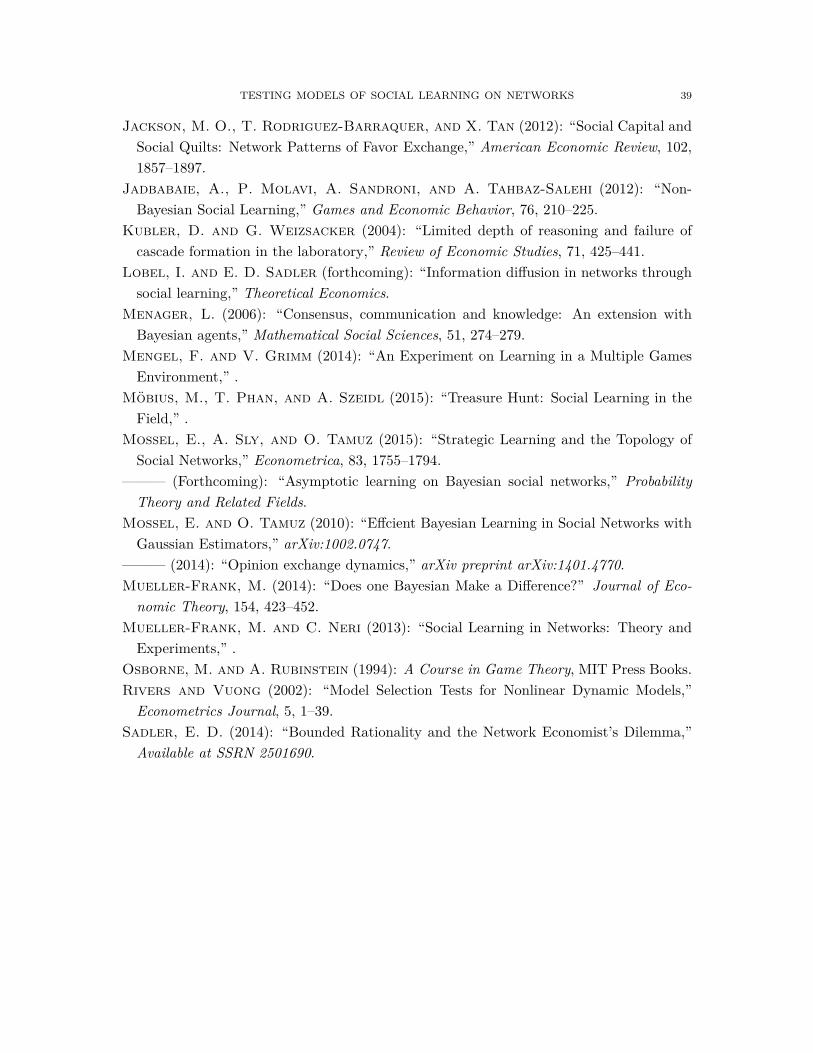
TESTING MODELS OF SOCIAL LEARNING ON NETWORKS 39
Jackson, M. O., T. Rodriguez-Barraquer, and X. Tan (2012): “Social Capital andSocial Quilts: Network Patterns of Favor Exchange,” American Economic Review, 102,1857–1897.
Jadbabaie, A., P. Molavi, A. Sandroni, and A. Tahbaz-Salehi (2012): “Non-Bayesian Social Learning,” Games and Economic Behavior, 76, 210–225.
Kubler, D. and G. Weizsacker (2004): “Limited depth of reasoning and failure ofcascade formation in the laboratory,” Review of Economic Studies, 71, 425–441.
Lobel, I. and E. D. Sadler (forthcoming): “Information diffusion in networks throughsocial learning,” Theoretical Economics.
Menager, L. (2006): “Consensus, communication and knowledge: An extension withBayesian agents,” Mathematical Social Sciences, 51, 274–279.
Mengel, F. and V. Grimm (2014): “An Experiment on Learning in a Multiple GamesEnvironment,” .
Möbius, M., T. Phan, and A. Szeidl (2015): “Treasure Hunt: Social Learning in theField,” .
Mossel, E., A. Sly, and O. Tamuz (2015): “Strategic Learning and the Topology ofSocial Networks,” Econometrica, 83, 1755–1794.
——— (Forthcoming): “Asymptotic learning on Bayesian social networks,” ProbabilityTheory and Related Fields.
Mossel, E. and O. Tamuz (2010): “Effcient Bayesian Learning in Social Networks withGaussian Estimators,” arXiv:1002.0747.
——— (2014): “Opinion exchange dynamics,” arXiv preprint arXiv:1401.4770.Mueller-Frank, M. (2014): “Does one Bayesian Make a Difference?” Journal of Eco-nomic Theory, 154, 423–452.
Mueller-Frank, M. and C. Neri (2013): “Social Learning in Networks: Theory andExperiments,” .
Osborne, M. and A. Rubinstein (1994): A Course in Game Theory, MIT Press Books.Rivers and Vuong (2002): “Model Selection Tests for Nonlinear Dynamic Models,”Econometrics Journal, 5, 1–39.
Sadler, E. D. (2014): “Bounded Rationality and the Network Economist’s Dilemma,”Available at SSRN 2501690.

TESTING MODELS OF SOCIAL LEARNING ON NETWORKS 40
Tables
Table 1. Fraction of observations for which the complete informationBayesian model differs with the DeGroot alternative
[1] [2] [3]
Network Uniform Degree Eigenvector
1 0.00% 0.00% 0.00%
2 0.00% 0.00% 6.80%
3 11.34% 22.68% 12.47%
[1] [2] [3]
Network Uniform Degree Eigenvector
1 6.95% 11.15% 6.95%
2 10.04% 10.39% 10.39%
3 9.63% 10.69% 10.69%
Panel A: Networks from Choi et al. (2005, 2009)
Panel B: Networks Selected in This Paper
Notes: Fraction of observations for which the complete information Bayesianmodel differs with the DeGroot alternative. In Panel A, network 1 is the“complete network”, network 2 is the “directed network”, and network 3 is the“incomplete network” of Choi et al. (2005, 2009). In Panel B, network 3 hasidentical paths for Bayesian and both uniform and degree DeGroot alternatives.We chose this network to pit Bayesian against eigenvector weighting.

TESTING MODELS OF SOCIAL LEARNING ON NETWORKS 41
Table 2. One-sided tests with the null of Bayesian learning against eachalternative of the DeGroot model for the network-level analysis
[1] [2] [3] [4]H0 H1 All networks Network 1 Network 2 Network 3
Bayesian Uniform 0.0000*** 0.0000*** 0.0000*** 0.0001***Bayesian Eigenvector 0.0000*** 0.0000*** 0.0001*** 0.0151**Bayesian Degree 0.0000*** 0.0000*** 0.0001*** 0.0151**Uniform Degree 0.9999*** 0.9999*** 0.9482* 0.9999***Uniform Eigenvector 0.9999*** - 0.9458* 0.9999***Degree Eigenvector 0.0000*** 0.0000*** - -
Notes: The test statistic is the normalized difference in the divergence function of the null and the alternative model. We show the probability that the test statistic is less than zero, estimated via bootstrap with replacement at thesession level.

TESTING MODELS OF SOCIAL LEARNING ON NETWORKS 42
Table 3. Incomplete information parameter estimates and correspondingdivergences for the network-level analysis
[1] [2] [3]πu πd πe
Point Estimate 0.00 0.00 0.00Standard Error (0.08) (0.12) (0.09)
[1] [2] [3]Divergence 0.1198 0.1413 0.1343
Standard Errors (0.0096) (0.0102) (0.0099)
[1] [2] [3]πu πd πe
Point Estimate 0.00 0.00 0.00Standard Errors (0.2834) (0.2620) (0.3139)
[1] [2] [3]Divergence 0.1798 0.1721 0.1831
Standard Errors (0.0107) (0.0106) (0.0105)
Panel C: Incomplete information point estimates, no common knowledge
Panel A: Incomplete information point estimates
Panel B: Incomplete information expected divergence
Panel D: Incomplete information divergence, no common knowledge
Notes: Columns 1, 2 and 3 refer to the alternative models of uniform, degree and eigenvectorcentrality weighting, respectively. Standard errors are constructed by bootstrapping withreplacement at the session level.

TESTING MODELS OF SOCIAL LEARNING ON NETWORKS 43
Table 4. One-sided tests with the null of Bayesian learning against eachalternative of the DeGroot model for the individual-level analysis
[1] [2] [3] [4]H0 H1 All networks Network 1 Network 2 Network 3
Bayesian Uniform 0.0000*** 0.0000*** 0.0000*** 0.0000***Bayesian Eigenvector 0.0000*** 0.0000*** 0.0000*** 0.0000***Bayesian Degree 0.0000*** 0.0000*** 0.0000*** 0.0000***Uniform Degree 0.9999*** 0.9999*** 0.9757** 0.9999***Uniform Eigenvector 0.9999*** 0.9999*** 0.9999*** 0.9999***Degree Eigenvector 0.8074 0.2460 0.9990*** 0.6451
Notes: The test statistic is the normalized difference in the divergence function of the null and the alternative model. We show the probability that the test statistic is less than zero, estimated via bootstrap with replacement at thesession level. When comparing DeGroot alternatives we use all observations, since there is no notion of zeroprobability information sets. When comparing complete information Bayesian to a DeGroot alternative, we only usehistories on which a Bayesian agent has not reached a zero probability information set.

TESTING MODELS OF SOCIAL LEARNING ON NETWORKS 44
Table 5. Information dominance
[1] [2]H1 Observations Percent Bayesian
Uniform 98 17.35%Degree 46 17.39%Eigenvector 98 17.35%Notes: Observations are the number of cases wherethere are discrepancies between the parent node action(which, from t > 3 has the property that under theBayesian model the peripheral node should follow theparent node) and the action that the alternative modelprescribes for the peripheral node. The percentBayesian presents the share of observations in whichthe peripheral nodes followed the Bayesian nodeaction.

TESTING MODELS OF SOCIAL LEARNING ON NETWORKS 45
Table 6. Cases that encounter zero probability information sets
[1] [2] [3]Network % Individuals % Sessions % Observations
1 47.97% 72.63% 43.90%2 54.29% 73.68% 46.15%3 33.06% 64.29% 34.66%
[1] [2] [3]Network % Individuals % Sessions % Observations
1 35.79% 72.63% 37.29%2 37.14% 68.42% 39.85%3 26.94% 64.29% 31.45%
[1] [2] [3]Network % Individuals % Sessions % Observations
1 34.14% 67.37% 37.02%2 38.05% 70.53% 40.70%3 25.92% 62.86% 30.89%
[1] [2] [3]Network % Individuals % Sessions % Observations
1 36.09% 72.63% 38.00%2 38.05% 70.53% 40.70%3 25.92% 62.86% 30.89%
Panel A: Complete Information
Panel B: Uniform Weighting Alternative
Panel C: Degree Weighting Alternative
Panel D: Eigenvector Weighting Alternative
Notes: All percentages computed using the π that minimizes the share of data units(individuals, sessions or observations) that reach zero probability information sets.
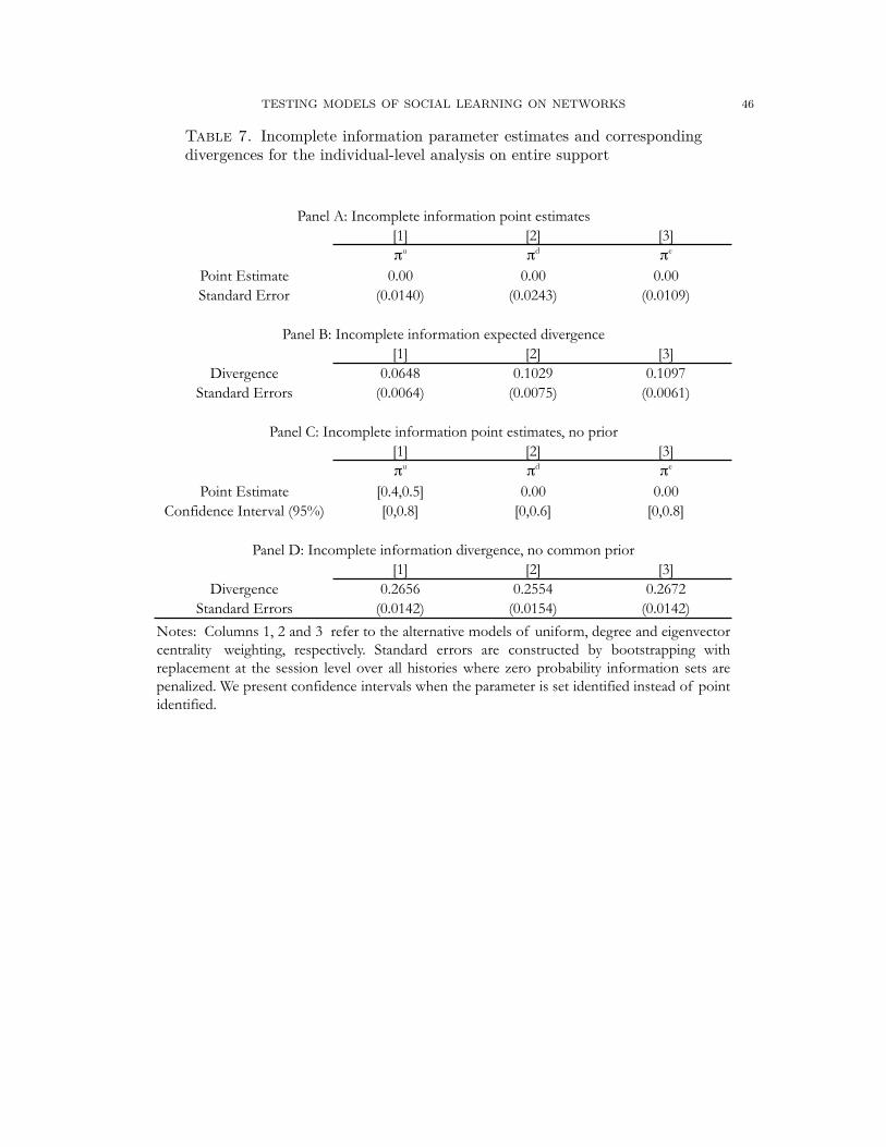
TESTING MODELS OF SOCIAL LEARNING ON NETWORKS 46
Table 7. Incomplete information parameter estimates and correspondingdivergences for the individual-level analysis on entire support
[1] [2] [3]πu πd πe
Point Estimate 0.00 0.00 0.00Standard Error (0.0140) (0.0243) (0.0109)
[1] [2] [3]Divergence 0.0648 0.1029 0.1097
Standard Errors (0.0064) (0.0075) (0.0061)
[1] [2] [3]πu πd πe
Point Estimate [0.4,0.5] 0.00 0.00Confidence Interval (95%) [0,0.8] [0,0.6] [0,0.8]
[1] [2] [3]Divergence 0.2656 0.2554 0.2672
Standard Errors (0.0142) (0.0154) (0.0142)
Panel A: Incomplete information point estimates
Panel B: Incomplete information expected divergence
Panel C: Incomplete information point estimates, no prior
Panel D: Incomplete information divergence, no common prior
Notes: Columns 1, 2 and 3 refer to the alternative models of uniform, degree and eigenvectorcentrality weighting, respectively. Standard errors are constructed by bootstrapping withreplacement at the session level over all histories where zero probability information sets arepenalized. We present confidence intervals when the parameter is set identified instead of pointidentified.

TESTING MODELS OF SOCIAL LEARNING ON NETWORKS 47
Table 8. Incomplete information parameter estimates and correspondingdivergences for the individual-level analysis on Bayes-feasible histories
[1] [2] [3]πu πd πe
Point Estimate 0.00 0.00 0.90Standard Error (0.3214) (0.2765) (0.3102)
[1] [2] [3]Divergence 0.0685 0.1068 0.1177
Standard Errors (0.0155) (0.0145) (0.0151)
[1] [2] [3]πu πd πe
Point Estimate [0.9,1] 0.90 0.90Confidence Interval (95%) [0,1] [0,1] [0,1]
[1] [2] [3]Divergence 0.2750 0.2762 0.2769
Standard Errors (0.0148) (0.0148) (0.0152)Notes: Columns 1, 2 and 3 refer to the alternative models of uniform, degree and eigenvectorcentrality weighting, respectively. Standard errors are constructed by bootstrapping withreplacement at the session level over all histories where any Bayesian agent has not yet reached azero probability information set. Therefore, zero probability information sets are not penalized.We present confidence intervals when the parameter is set identified instead of point identified.
Panel A: Incomplete information point estimates
Panel B: Incomplete information expected divergence
Panel C: Incomplete information point estimates, no common prior
Panel D: Incomplete information divergence, no common prior

TESTING MODELS OF SOCIAL LEARNING ON NETWORKS 48
Table 9. Overweighting information received through multiple channels
All Restricted All Restricted All Restricted All Restricted[1] [2] [3] [4] [5] [6] [7] [8]
Signal .4974*** .5351*** .3965*** .4429*** .5725*** .6204*** .6017*** .677***[.0218] [.0279] [.017] [.0223] [.0169] [.0211] [.0159] [.0201]
Direct .7735*** .7485*** .775*** .8048*** .9125*** .8913*** .8954*** .9078***[.0311] [.0438] [.0323] [.0384] [.0335] [.0425] [.0381] [.0475]
One Way .3157*** .2609*** .7056*** .8189*** 0.0461 -0.0614 .1306*** .077*[.0405] [.0542] [.0363] [.0486] [.035] [.0421] [.0368] [.0447]
Two Ways .2177*** .1751*** .3582*** .4096*** .0797* 0.024 .1985*** .1841***[.0355] [.0424] [.0337] [.0338] [.0421] [.0449] [.0459] [.0519]
TwoWays > OneWayt-statistic -1.97 -1.557 -8.653 -8.136 0.7675 1.925 1.481 2.215Probability 0.9741 0.9386 1 1 0.2224 0.0287 0.071 0.0146N 1750 1271 1750 1271 1750 1271 1750 1271R -squared 0.4724 0.373 0.5322 0.4632 0.588 0.5453 0.5974 0.5571
Note: Robust standard errors, clustered at the village by game level, in brackets. Ouctome variable is action in round 3. "Direct" is the average signal of direct neighbors, "One Way" is the average signal of indirect neighbors only thorugh one direct neighbor, and "Two Ways" is the average signal of indirect neighbors thorugh two direct neighbors. Column (1) is the regression with all data. Column (2) is the regression restricting to treatments that are informative for the comparisons Bayesian - Degree and Bayesian - Uniform. * p<.1, ** p<.05, *** p<.01
Data Bayesian Degree Uniform

TESTING MODELS OF SOCIAL LEARNING ON NETWORKS 49
Table 10. Re-incorporation of previously-observed historical information
All Restricted All Restricted All Restricted All Restricted[1] [2] [3] [4] [5] [6] [7] [8]
Signal .4284*** .4573*** .4729*** .5264*** .4507*** .482*** .5694*** .6468***[.0347] [.0425] [.0286] [.0356] [.032] [.0359] [.0307] [.0357]
Direct .7508*** .7011*** .8095*** .8007*** .8436*** .8167*** .7576*** .7275***[.0363] [.0471] [.0285] [.0346] [.0402] [.0489] [.0391] [.0492]
Indirect New .2455*** .1803*** .3768*** .3489*** .1558*** .0883** .2548*** .2063***[.0331] [.0377] [.0261] [.0317] [.0333] [.0384] [.0283] [.0338]
Indirect Repeated .1715*** .1669*** .1029*** .0801* .2463*** .2619*** .1724*** .1554***[.0416] [.048] [.0354] [.0427] [.0398] [.0447] [.0417] [.0492]
N 1587 1250 1587 1250 1587 1250 1587 1250R -squared 0.4628 0.3958 0.4953 0.4135 0.5819 0.5475 0.5945 0.5687
Note: Robust standard errors, clustered at the village by game level, in brackets. Ouctome variable is action in round 3. "Direct" is the average signal of direct neighbors, "Indirect New" is the average signal of indirect neighbors that provide new information, and "Indirect Repeated" is the average signal of indirect neighbors that do not provide new information. Column (1) is the regression with all data. Column (2) is the regression restricting to treatments that are informative for the comparisons Bayesian - Degree and Bayesian - Uniform. * p<.1, ** p<.05, *** p<.01
Data Bayesian Degree Uniform

TESTING MODELS OF SOCIAL LEARNING ON NETWORKS 50
Appendix A. Bayesian Learning Algorithm in Complete and IncompleteInformation Models
In this appendix, we describe the algorithm for computing the actions under the as-sumption of complete information Bayesian agents.
A.1. Setup. We follow the notation on Osborne and Rubinstein (1994) and Geanakoplos(1994), modeling agents’ information in the experiment by means of dynamically consis-tent models of action and knowledge (DCMAK), a natural multi-period generalization ofAumann (1976). Following Geanakoplos (1994), a DCMAK consists of a set of states of theworld ω ∈ Ω, information functions Pi,t : Ω → 2Ω, and action functions ai,t : Ω → 0, 1.In what follows, we will define these objects for our experimental setup, which we will useto calculate the predicted behavior of Bayesian agents ai,t (ω).
A.2. States of the world. In both the complete and incomplete information models, wemodel agents information as partitions over ω ∈ Ω, where ω = (ω1, ω2. . . . , ωn) is the vectorof agents’ initial private information. In the complete information case, ωi ∈ 0, 1 denoteswhether they observe a yellow ball (ωi = 1) or blue (ωi = 0); i.e., Ω = S = 0, 1n. In theincomplete information case (where players don’t know if their neighbors are Bayesian orDeGroot types) we model the state of the world as ωi = (si, ηi) where si ∈ 0, 1 is thecolor of the observed ball, and ηi ∈ 0, 1 denotes agent i′s type: she is either a Bayesiantype (ηi = 1) who guesses the most likely state following Bayes’ rule, or a DeGroot agent(ηi = 0) who decides her guess based on a weighted average of her neighbors’ guesses (weconsider the 3 variants mentioned: uniform, degree and eigenvector centrality weighting).
On both complete and incomplete information models, Bayesian agents have a commonprior belief over states ω ∈ Ω, conditional on the realization of θ ∈ 0, 1 (i.e., which baghas been chosen), which we denote by ρ (ω | θ). In the complete information model ω = s
and all agents are of the Bayesian type ηi = 1 at all states, and hence
(A.1) ρ (ω | θ) = ρ (s | θ) := p
∑jsj
θ (1− pθ)n−∑
jsj for θ ∈ 0, 1 , ω ∈ Ω,
where pθ = P (si = 1 | θ). In our experiment, pθ = 5/7 if θ = 1 and pθ = 2/7 if θ = 0. In theincomplete information model, ω = (s, η) where η = (η1, η2, . . . , ηn) is a type profile (thecomplete description of every agent’s type), and we assume that agents have a common priorover agents’ types as well, which are assumed to be i.i.d. across agents and independent ofobserved signals;
(A.2) ρ (s, η | θ) := p
∑jsj
θ (1− pθ)n−∑
jsj
[π∑
jηj (1− π)n−
∑jηj
],
where π := P (ηi = 1). The set of all type configurations is denoted by H = 0, 1n, andin this model, Ω := S ×H = 0, 1n × 0, 1n.

TESTING MODELS OF SOCIAL LEARNING ON NETWORKS 51
A.3. Recursive definition of information and action functions. The function Pi,t (ω) ⊆Ω denotes the information set of agent i at round t, under state ω. At round t = 1, agenti only observes ωi out of state ω, and hence, her information set is:
(A.3) Pi,1 (ω) :=ω′ ∈ Ω : ω′i = ωi
,
i.e., the possible states of the world are those compatible with the private information shehas received (which includes her signal si ∈ 0, 1 and her type). Based on this information,all agents choose to match their signal; i.e.,
(A.4) ai,1 (ω) := si.
For t > 1 we compute Pi,t (ω) and ai,t (ω) inductively, for each ω ∈ Ω. In our experi-mental setup, at round t agent i observes all the actions taken by her neighbors j ∈ N (i)(including herself) up to s = t − 1. Therefore, the states of the world that are consistentwith agent i’s observations (her information set) are
(A.5) Pi,t (ω) :=ω′ ∈ Ω : ω′i = ωi and aj,s
(ω′)
= aj,s (ω) for all j ∈ N (i) , s ≤ t− 1.
Clearly, we have Pi,t (ω) ⊆ Pi,t−1 (ω) for all i, ω ∈ Ω (i.e., Pi,t (·) corresponds to a filtra-tion).24 The round t action function ai,t (ω) is then given by:
(A.6) ai,t (ω) :=
1Ii,t (ω) > 1
2
if Ii,t (ω) 6= 1
2
ai,t−1 (ω) if Ii,t (ω) = 12
,
where Ii,t (ω) is the “belief index” at state ω, which depends on the agents’ type. If agenti is Bayesian (i.e., under the complete information model, or if τi = 1 in the incompleteone), then Ii,t (ω) := P (θ = 1 | Pi,t (ω)), which is calculated using Bayes rule conditioningon the event B = Pi,t (ω):
(A.7) P (θ = 1 | Pi,t (ω)) :=∑ω′∈Pi,t(ω) ρ (ω′ | θ = 1)∑
ω′∈Pi,t(ω) ρ (ω′ | θ = 1) + ρ (ω′ | θ = 0)
When i is not Bayesian at ω, then Ii,t (ω) :=∑nj=1 Tijaj,t−1 (ω) where [Tij ]ij are the DeG-
root weights (which are T u, T d or T e as in equations (2.1), (2.2), and (2.3), depending onthe assumed alternative type).
A.4. Numerical Implementation. The algorithm used is based on the inductive stepdefined above, calculating iteratively the objects Pi,t (ω) and ai,t (ω) for all i, t and ω, forboth the complete and incomplete information models.
Algorithm 1. Bayesian Learning Algorithm (Complete Information case)Input: An n−person network G = (V,E) with adjacency matrix An×n
24We can also define Pi,t recursively, starting at Pi,1 as in A.3, and for t ≥ 1 let Pi,t (ω) := Pi,t−1 (ω) ∩ω′ ∈ Ω : aj,t−1 (ω′) = aj,t−1 (ω′) for all j ∈ N (i)

TESTING MODELS OF SOCIAL LEARNING ON NETWORKS 52
Outputs: Information and action functions Pi,t (ω) and ai,t (ω)Step 1: Initialize algorithm by defining:(1) State space Ω = 0, 1n
(2) Measures ρ (ω | θ) according to A.2, for θ ∈ 0, 1(3) Information functions Pi,1 (ω) and actions ai,1 (ω) according to A.3 and A.4 for all
i = 1, . . . n and ω ∈ Ω.Step t > 1: Given (Pi,s (ω) , ai,s (ω))i=1,...n,s=1,...t−1,ω∈Ω calculate Pi,t (ω) and ai,t (ω) forall i and ω ∈ Ω according to A.5 and A.6, where Ii,t (ω) = P (θ = 1 | Pi,t (ω)) as in equation(A.7).
Algorithm 2. Bayesian Learning Algorithm (Incomplete Information case)Inputs:(1) An n−person network G = (V,E) with adjacency matrix An×n(2) A row stochastic matrix of DeGroot weights Tn×n(3) Probability π ∈ [0, 1]
Output: Information and action functions Pi,t (ω) and ai,t (ω)Step 1: Initialize algorithm by defining:(1) State space Ω = S ×H = ω = (s, η) where s ∈ S := 0, 1n , η ∈ H := 0, 1n(2) Measures ρ (ω | θ) = ρ (s, η | θ) according to A.2, for θ ∈ 0, 1(3) Information functions Pi,1 (ω) and actions ai,1 (ω) according to A.3 and A.4 for all
i = 1, . . . n and ω ∈ Ω.Step t > 1: Given (Pi,s (ω) , ai,s (ω))i=1,...n,s=1,...t−1,ω∈Ω calculate Pi,t (ω) and ai,t (ω) forall i and ω ∈ Ω according to A.5 and A.6, where Ii,t (ω) = P (θ = 1 | Pi,t (ω)) if ηi = 1 andIi,t (ω) =
∑j Tijaj,t (ω) if ηi = 0.
It is worth noting that an alternative way of modeling the knowledge structure is byincluding the true state θ in the description of the state of the world; i.e., define ω = (θ, s)in the complete information case, and ω = (θ, s, η) in the incomplete information case,which would need the definition of just one common prior ρ (ω), instead of having to defineit conditional on θ. While this would perhaps be a better fit for most epistemic models,the description of the algorithm is slightly easier in our model, given the fact that ω = s
in the complete information model, and ω = (s, η) in the incomplete information modelsare, respectively, sufficient statistics for the actions sequence of players, since θ is never inany information set of any of the players, significantly reducing the relevant state space (infact, these are the minimal state spaces we can consider, exactly because of sufficiency).
A.5. Complexity. The decision problem we are interested in is determining whether anagent i in time period t given a history always picks the same action under a proposed

TESTING MODELS OF SOCIAL LEARNING ON NETWORKS 53
algorithm as under the Bayesian model with trembles. We conjecture that the problem isNP-hard, which we are investigating in ongoing work. This means that the computationalproblem is at least as hard as NP-complete problems.25 Whether there may or may notbe polynomial time solutions for NP-hard problems is open; if P 6= NP, then none wouldexist. The computer science literature studying Bayesian learning networks shows thatobtaining the probabilities is NP-hard (Cooper, 1990) in any given network of events. Inthis context, the networks are networks of events. Translating our framework into thissetup involves constructing a network of belief states for each individual in the networkand each time period, so a node in the Bayesian learning network would be a pair (i, t),so the size of it would be N · T . Our ongoing work seeks to extend their argument to ourdecision problem which involves checking that the action taking by each person in each timeperiod is identical when comparing a proposed algorithm with the true Bayesian learningmodel. The intuition is that the associated learning network is growing exponentially inthe number of periods and individuals, and therefore, for any algorithm there can be someaction sequence such that to be able to decide whether individual i at time t, given thehistory, needs to decide whether to guess 0 or 1, one needs all the probabilities. Basedon Cooper (1990), which applies to a broader class of networks (and therefore will haveweakly worse complexity), we conjecture that the argument for our sub-class of networkswill also be NP-hard.
Let Ωt be the the set of states that agent i has to integrate over at time t. The basicalgorithm (in this general version) involves two states: the indicator function of the setPi (ω) for each ω ∈ Ωt and the action function ai,t (ω). We define
σt(i, ω, ω′
):=
1 if ω′ ∈ Pi,t (ω)
0 otherwise
and
αt (i, ω, t) := ai,t (ω)
to calculate the objects Pi,t (ω) and ai,t (ω) numerically, as in appendix A.4. To calculatethem, we then have to loop across # (Ωt)×# (Ωt) states for each (i, t) to update σt to σt+1
and # (Ωt) to update αt. The number of operations is then∑t
∑i
(∑w∈Wt
(k +
∑w∈Wt
k))
where k is the number of computations done in each step. In the deterministic completeinformation model (without trembles), Ωt = S = 0, 1n and then
Computations = nT (2n) (1 + 2n) k = Θ (T4n) .
25A problem is said to be NP-complete if (a) it is in NP, which is to say that a given solution can be verifiedin polynomial time, and (b) it is NP-hard, so that any NP problem can be converted to this problem inpolynomial time.

TESTING MODELS OF SOCIAL LEARNING ON NETWORKS 54
In the incomplete information model, it is nT (4n) (1 + 4n) k. The ratio between thecomplete and incomplete information models is then
nT (4n) (1 + 4n) knT (2n) (1 + 2n) k = 2n 1 + 4n
1 + 2n ≈ 4n
So, for a network of n = 7, the relative complexity of the incomplete information modelapproximately 16, 258.
The trembling hand complete information model needs agents to integrate over 2n(t−1)
states, at least, in each round; since there is no longer a deterministic mapping betweeninformation sets and signal profiles, agent i needs to integrate over the actions of otheragents. Although agent i actually does not observe the information of n − di agents, forrounds t ≥ 3 we have to have to calculate her beliefs about those agents’ informationsets. The partitional model presented in appendix A.4 does not suffer this problem, bycalculating beliefs on all states, which we do here as well. Therefore # (Wt) = 2n(t−1) andthe number of calculations is
k∑i
t−1∑t=1
2n(t−1)(k + 2n(t−1)
)= k
∑i
(T−1∑t=1
2n(t−1) +T−1∑t=1
22n(t−1))
k∑i
[(2nT − 2n
2n − 1
)+ 22nT − 22n
2n − 1
]= n
(2nT − 2n
)2n − 1
(1 +
(2nT − 2n
) 2n − 122n − 1
)= Θ
(4n(T−1)
)Therefore, the ratio between the two is approximately
n2n(T−1)[k + 2(T−1)
]nT (2n) (k + 2n) ≈ 1
T× 4n(T−2),
and for the incomplete information model, the equivalent ratio is
n4n(T−1)(1 + 4n(T−1)
)nT (4n) (1 + 4n) .

TESTING MODELS OF SOCIAL LEARNING ON NETWORKS 55
Online Appendices
Appendix B. Online Appendix: Filtering
Here we describe a filter to estimate, in the incomplete information model, the probabilitythat an agent is Bayesian given the data that the researcher has in hand, under the networklevel approach. The objective of this section is to estimate
Fi := P (i is Bayesian | π, experimental data in room r) .
To simplify the exposition, we drop the subscripts for the particular room r, the alternativemodel used, m and the prior probability of players being Bayesian, π ∈ [0, 1]. Let [k] =1, 2, . . . , k for any k ∈ N, T = Tr be the number of rounds played, and
aobsi,t
i∈[n],t∈[T ]
denote the (panel) data set of player choices, which include the signals drawn at t = 1(since sobsi ≡ aobsi,1 ). Given a type profile η ∈ H, define the observation level divergenceDi,t (η) :=
∣∣∣ai,t (sobs, η)− aobsi,t ∣∣∣ for all i ∈ [n] and t > 1. The room level divergence of typeprofile η is defined as D (η) := 1
n(T−1)∑i,t>1Di,t (η).
In the network level approach, we treat the data generating process as follows: astate ω ∈ Ω = S × H is drawn at t = 1, and agents play according to the equilib-rium path sequence ai,t (ω). The researcher knows the actual signal endowment s = sobs
(i.e., the color of the balls drawn in the experiment), and the panel of actions chosen byall agents, which we denote by
aobsi,t
i∈[n],t∈[T ]
. Formally, the information set of the re-
searcher, PR ⊆ Ω, restricts the set of states to those consistent with the observed data; i.e.PR :=
ω = (s, η) ∈ S ×H : ai,t (ω) = aobsi,t for all i ∈ [n] , t ≤ T
. Therefore, the only re-
maining uncertainty is the type profile η ∈ H, and the researcher information can be betterdescribed as restrictions over possible type profiles, denoted by
HR := projHPR =η ∈ H : ai,t
(sobs, η
)= aobsi,t for all i ∈ [n] , t ∈ [T ]
.
In this appendix, we are particularly interested in calculating the posterior probability thatagent i is Bayesian, given a prior probability π,
Fi (π) := P(ηi = 1 |
aobsi,t
, π).
If there exists some type profile η∗ that is consistent with the observed data (i.e. HR 6=∅), then this can be easily calculated using Bayes’ rule:
Fi (π) = P(ηi = 1 | η ∈ HR
)=∑η∈HR:ηi=1 P
(η | sobs
)∑η∈HR P (η | sobs)
=∑η∈HR:ηi=1 (π/1− π)nη∑η∈HR (π/1− π)nη
.

TESTING MODELS OF SOCIAL LEARNING ON NETWORKS 56
Since P (η) = π∑
jηj (1− π)n−
∑jηj = (1− π)n
(π
1−π
)nη, where η := 1
n
∑j ηj . While
tractable, this exercise is impossible in most of our experiments: as Table 6 shows, in atleast 63% of experiments, no type profile η∗ ∈ H exist that could rationalize the observeddata (i.e HR = ∅) regardless of network topology chosen and the alternative DeGrootaction type for the incomplete information model.
If we maintain the network level approach interpretation, an alternative is to add “trem-bles” to ensure full support over possible action sequences ai,ti,t. Formally, let ai,t ∈ 0, 1be the (random) choice of agent i at round t . The key object we need to model is theprobability of observing the dataset
aobsi,t
i,t
if the state is ω =(sobs, η
)A (η) := P
(ai,t = aobsi,t for all i ∈ [n] , t ∈ [T ]|ω =
(sobs, η
))so A (η) is the likelihood function of type profile η (treated as a parameter) given theobserved data. Given A (η), we can calculate Fi by first getting the posterior distributionover type profiles, using Bayes’ rule
P(η |aobsi,t
i,t
)= P (η)A (η)∑
η∈H P (η)A (η)
and then calculating the probability of ηi = 1 under it,
Fi := P(ηi = 1 |
aobsi,t
i,t
)=
∑η:ηi=1
P(η |aobsi,t
i,t
)
=∑η:ηi=1 (π/1− π)nηA (η)∑η (π/1− π)nηA (η)
.
Our leading example of a model of trembles will be the independent trembles model,parametrized by a constant ε ∈ (0, 1). Formally, given a type profile η ∈ H, we assume(1) ai,1 = sobsi with probability 1 for all i (2) ai,t = ai,t
(sobs, η
)with probability (1− ε),
which is i.i.d across players and rounds. Formally,
A (η) := ε∑
i,t>1 Di,t(η) (1− ε)n(T−1)−∑
i,t>1 Di,t(η),
where Di,t (η) :=∣∣∣aobsi,t − ai,t (sobs, η)∣∣∣ is the theoretical observation divergence under state
ω =(sobs, η
). It can be expressed in a more familiar way as
A (η) =[εD(η) (1− ε)1−D(η)
]n(T−1)= (1− ε)n(T−1)
(ε
1− ε
)n(T−1)D(η).
A nice feature is that the posterior distribution over type profiles is directly related to itsmeasured divergence:
P(η |aobsi,t
i,t
)∝ P (η)×
(ε
1− ε
)n(T−1)D(η),

TESTING MODELS OF SOCIAL LEARNING ON NETWORKS 57
and hence,
(B.1) Fi = 1Λ (π, ε)
∑η:ηi=1
(π
1− π
)nη ( ε
1− ε
)n(T−1)D(η),
where Λ (π, ε) :=∑η (π/1− π)nη (ε/1− ε)n(T−1)D(η) is proportional to the probability of
the researcher’s information set over type profilesHR26. One may observe that type profilesthat do not explain the data well (if D (η) is high) are given a lesser weight in the posteriordistribution if ε < 1
2 , so that the filtered probability of i being Bayesian depends cruciallyon how much is this evidenced by the data.
Appendix C. Online Appendix: Stuck Nodes and Complete Binary Quilts
C.1. Setup. We present a simple growing sequence of networks that illustrates the resultsof Proposition 2.1. In this example, there is asymptotic efficiency under communicationDeGroot models and action Bayesian models, but asymptotic learning fails and consensusdoes not occur with action DeGroot models
We say a network T = (V,E) is a binary tree if it is a rooted tree where every nodehas either two children, or none (i.e., a terminal node).27 The level of a node j ∈ V is theshortest path distance to the root node i0. The set of nodes of level d is denoted by Ld.28
Define the depth of a network d to be the maximum distance possible from the root node.A complete binary tree of depth d is a binary tree Td =
(Vd, Ed
)where every terminal
node has depth d. Note that in this network, every node (other than the root) has 1 sibling(a node that has the same parent) to which it is not connected.
Given Td, we define a complete binary quilt of depth d to be a network Qd = (Vd, Ed),super-graph of Td, where Vd = Vd and Ed = Ed ∪ ij : i and jare siblings, as illustratedin Figure C.1.
1
2 3
4 5 6 7
8 9 10 11 12 13 14 15
(a) Td
1
2 3
4 5 6 7
8 9 10 11 12 13 14 15
(b) Qd
Figure C.1. Complete binary tree Td and complete binary quilt Qd (d = 3)
26Namely, P(HR)
= Λ (π, ε)×[(1− π) εT−1]n
.27A terminal node, or leaf, is a node in a tree with only one neighbor (i.e., it has degree 1).28Formally, Ld := j ∈ V : d (i0, j) = d where d (i, j) is the length of the shortest path between i and j(which exists, given that T is a connected graph).

TESTING MODELS OF SOCIAL LEARNING ON NETWORKS 58
The motivation for the graph structure comes from Jackson et al. (2012), who study net-work architecture that arise as equilibria in favor-exchange games. They show that thesenetworks are social quilts. A social quilt is a patchwork of substructures (e.g., triangles)pasted together in specific ways: the substructures do not share edges, only vertices. Fromthe applied perspective, this speaks to how the incentives to overcome contractual incom-pleteness, or lack of formal insurance, influence how well a society may engage in sociallearning. If graphs are constructed as equilibria of risk-sharing or favor-exchange games,then they may have such quilt-like substructures. However, at the same time, because offixed costs in building relationships, the resulting pattern of relationships will also be thenetwork on which information travels.
1
2 3 4 5
6 7(a)
1
2 3 4 5
6 7 −→
1
2 3 4 5
6 7(b)
Figure C.2. In Panel A, two nodes are stuck for all periods t ∈ N, eventhough 5 of the 7 nodes have received the correct signal. In Panel B, in thefirst period, 4 nodes receive the correct signal, and after one node switches,3 are stuck.
This family of networks is prone to having stuck nodes, just as we saw when studyingtopology 3, which is a particular sub-case. Panel A of Figure C.2 illustrates the problem.Assume that for some subtree of level d − 1 of Qd (i.e., where the siblings are terminalnodes), which connects to the rest of the network through its parent node (as in FigureC.2), we have the initial signal endowment shown in Panel A of Figure C.2. To get a lowerbound on the number of nodes that get stuck in the wrong action, we can simply assume

TESTING MODELS OF SOCIAL LEARNING ON NETWORKS 59
that the parent node of the subtree always chooses the right action for all rounds. However,even in this case, the nodes in the lower right triangle act in the same (wrong) mannerfor all periods, since they follow the DeGroot uniform weighting rule as in equation 2.1.Note that in large enough networks, taking an action that goes against the majority willbe almost surely be the same as taking the wrong action (since almost surely, most agentswill have observed the right signal as p > 1/2). We will use this equivalent definition ofstuckness for large networks in this application (i.e., a node i is stuck if ∃Ti :ai,t = 1 − θfor all t ≥ Ti)
Take a sequence of networks Qdd∈N of growing complete binary quilts. As d → ∞,there will be a non-vanishing fraction of subtrees with this initial configuration of signals.Following the argument of Panel A of Figure C.2, take the subgraph induced by levelsd− 2, d− 1 and d of Qd; i.e., subgraph Q′ induced by V ′ = Ld−2 ∪ Ld−1 ∪ Ld. It consistsof the union of 2d−2 connected components of 7 players, like the ones in panel A andB of Figure C.2. If d is big enough for the law of large numbers to kick in, there willbe approximately a fraction of p5 (1− p)2 of those components with signal configurationsas in Panel A, and each of these will have at least 2 players getting stuck choosing thewrong action. This already gives a non-zero lower bound on the fraction of agents thatwill never match their action to the true state of nature, even if the network is arbitrarilybig. In this case, the fraction of agents that get stuck in components like Panel A is atleast f = 1
4p5 (1− p)2 as d→∞.29
This example has demonstrated the following result. We say that a sequence of networksexhibits asymptotic learning if all but a vanishing share of nodes correctly guess the stateof the world.That asymptotic learning occurs with the Bayesian action model follows from Mossel et al.(Forthcoming), and that it occurs with DeGroot communication for this model followsfrom Corollary 1 of Golub and Jackson (2010). The result for the DeGroot action model isapparent from the previous example. To illustrate the severity of Proposition 2.1, in FigureC.3 we show lower bounds on the expected fraction of nodes that are stuck. These boundsare calculated by the argument following Figure C.2, replicating the bounds obtained forthe signal configurations of Panel A and B for all possible signal configurations of eachcomponent. Even with high quality signals (p = 0.7), at least 16% of nodes become stuckand do not asymptotically learn.
C.2. Estimating Upper and Lower Bounds on the Fraction Stuck.
29To see this, one can show that (1) # V = 2d+1 − 1; (2) there are 2d−2 components in V ′, each of 7nodes; and (3) at least 2 players out of Panel A-type components get stuck. Then, if d is large enough,we have that f ≈ 2× p5 (1− p2) 2d−2/(2d+1 − 1) = 1
4p5 (1− p)2 × (2d+1/2d+1 − 1). Since the second term
converges to 1 as d→∞, we get the desired expression.

TESTING MODELS OF SOCIAL LEARNING ON NETWORKS 60
Figure C.3. Bounds for fraction stuck
1
2 3
4 5 6 7
8 9 10 11 12 13 14 15
(a) Od (1)
1
2 3
4 5 6 7
8 9 10 11 12 13 14 15
(b) Od (2)
Figure C.4. Subgraphs Od (k) of Qd (d = 3).
C.2.1. Preliminary tools. We define Sd = i ∈ Vd : i gets stuck and let Nd = # (Vd), thenumber of nodes in Qd. Our object of interest is the random variable
Fd = Fraction of nodes in Qd that gets stuck ≡ #SdNd
.
Our objective is to get an asymptotic bound on Fd. Since we do not yet know whether Fdhas a limit for almost every realization, we define F and Fas
(C.1) F = lim infd→∞
Fd and F = lim supd→∞
Fd
which is well defined for all realizations of the sequence Fd, and so it is a well definedrandom variable. Namely, we want to get the tightest asymptotic lower and upper boundsfor the fraction of stuck nodes. Our objective is to get a number F ∈ [0, 1] such that F ≥ Fand F ≤ F almost surely; i.e., P
F ≤ F ≤ F ≤ F
= 1.
Define
Od (k) :=s=k⋃s=0
Ld−s

TESTING MODELS OF SOCIAL LEARNING ON NETWORKS 61
as the subgraph formed by the last k+ 1 levels of Qd. This subgraph is disconnected, witha lot of connected components, as pictured in Figure C.4. Let C be a generic connectedcomponent of Od (k); i.e., the induced subgraph of one of the connected components ofOd (k). For example, Panels A and B of Figure C.2 correspond to connected componentsof Od (2). Notice that in this example, each component of Od (2) is itself a complete binaryquilt of level 2. It is easy to see that in fact, the connected components of Od (k) are alsocomplete binary quilts; i.e., C = Qk (binary quilts of depth d′ = k). The key propertyof these subgraphs (and the reason for studying this family of networks) is that the onlyconnection between each component C and the rest of the graph is the parent node of thecomponent C, denoted by iC . Next, we see how this property allows us to study the localbehavior of the component, abstracting away from the rest of the network, in order to getbounds on the fraction of players stuck.
DefineΨd (k) = # Od (k) ∩ Sd
# Od (k)as the fraction of stuck nodes in Od (k),
Ψ (k) := lim infd→∞
# Od (k) ∩ Sd# Od (k) ,
andΨ (k) := lim sup
r→∞
# Or (k) ∩ Sr# Or (k) ,
which are also all well-defined random variables. These are the tightest asymptotic lowerand upper bounds on the fraction of nodes in Od (k) that get stuck.
Lemma C.1. For all k ∈ N, limd−→∞#Od(k)
Nd= 2k+1−1
2k+1 .
Proof. Let Ld = number of nodes in level r. Because of Qd being a complete binarynetwork, we have the following recursion for Ld :
Ld+1 = 2Ld and L0 = 1
from which it follows that
(C.2) Ld = 2d.
Therefore, the number of nodes in # Od (k) is then
# Od (k) =k∑s=0
# Ld−s = 2d−kk∑s=0
2s = 2d−k(
1− 2k+1
1− 2
)= 2d
(2k+1 − 1
2k
).
We also need to calculate Nd := # (Vd). Again, because of how Qd grows, it can be alsoeasily shown that
(C.3) Nd = 2d+1 − 1.

TESTING MODELS OF SOCIAL LEARNING ON NETWORKS 62
Now, we can state the result. Observe that
# Od (k)Nd
= 2d
2d+1 − 1
(2k+1 − 1
2k
)→d→∞
2k+1 − 12k .
as we wanted to show.
The following proposition is the key to understanding how to get bounds on F and Fby getting bounds on Ψ (k) and Ψ (k)
Proposition C.1. Suppose there exist functions ψ,ψ : N →[0, 1] such that for all k wehave
ψ (k) ≤ Ψ (k) ≤ Ψ (k) ≤ ψ (k) almost surely.
Then, for all k ∈ N almost surely,
(C.4) F ≥ 2k+1 − 12k+1 ψ (k) ,
and
(C.5) F ≤ 1−(
2k+1 − 12k+1
)[1− ψ (k)
].
Proof. Lets focus only on inequality C.4, since C.5 follows the same reasoning. See that
Fd = # Od (k)Nd
(# Od (k) ∩ Sd# Od (k)
)+ # Sd −Od (k)
Nd
≥ # Od (k)Nd
(# Od (k) ∩ Sd# Od (k)
),
so, for all realizations,
F = lim infd→∞
Fd ≥(
limd−→∞
# Od (k)Nd
)(lim infd→∞
(# Od (k) ∩ Sd# Od (k)
))=
(limr−→∞
# Od (k)Nd
)Ψ (k) = 2k+1 − 1
2k+1 Ψ (k) .
This, together with the fact that Ψ (k) ≥ ψ (k) almost surely, completes the proof.
Note that this proposition is true for any learning model (Bayesian or DeGroot). Thelearning model plays a role when calculating the bounds ψ and ψ. See that condition C.4and C.5 are bounds on F and F , which do not depend on k. Therefore, these are boundsfor all k. Moreover, the higher k, the tighter the bound.
C.2.2. Bounding the fraction stuck under uniform DeGroot. Without loss of generality, weassume that the true state of nature is θ = 1, which implies that as d→∞ the fraction ofnodes with true signals is p > 1
2 . The idea is simple: take a component C = (VC , EC) ⊂Od (k). As we mentioned before, the only connection between C and the rest of the graph isthrough the parent node iC (as seen in Figure C.4). Let SC = 0, 1NC be the set of signal

TESTING MODELS OF SOCIAL LEARNING ON NETWORKS 63
endowments for nodes in C. We look for a lower bound ψk
(s) for each signal endowmentrealization in C such that, when signal endowment is s, the fraction of stuck nodes in Cis larger that ψk (s) fraction of stuck nodes in C if the endowment is s ≥ ψ
k(s). If we can
find such ψk
(s), then we can use a law of large numbers to argue that
Ψ (k) ≥ ψ (k) ≡ Es∈SC
ψk
(s)
almost surely,
because the realizations of s in each component C is independent of each other. Likewise,if we can find a function ψk (s) to bound from above the fraction of stuck nodes,
Ψ (k) ≥ ψ (k) ≡ Es∈SC
ψk (s)
almost surely.
Imagine first that the signal endowment of the upper triangle in C is (0, 0, 0). Then,using Lemma 2.1 we know that the upper triangle of C will get stuck from period t = 1 on,and we can get the expected value of stuck nodes in C from there on. See that the fractionof nodes that get stuck in this component is only a function of the realization of s ∈ SC ,which is independent of the realization of the signal endowment of other components onOd (k)
When the signal endowment of the upper triangle in C is different from (0, 0, 0) , wemake use of the other property we know from C : the only connection to the rest of thegraph is through iC , the uppermost node in C. Therefore, a way of getting a lower boundon the number of nodes that get stuck, is assuming that from round t = 2 on, node iCknows the truth, and plays aiC ,t = 1 for all t ≥ 2. Intuitively, we are making the graph tohave the biggest effect possible in convincing nodes in C that θ = 1, which can only do bymaking aiC ,t = 1 for all rounds other than t ≥ 2. Once we have that, we can simulate thelearning model on C, and calculate ψk (s) and ψk (s).
There are two ways of calculating Es∈SC
ψk
(s)
:
(1) Doing it explicitly: This can be done for k = 2 and k = 3, because # SC (k = 4) =128.
(2) Monte-Carlo: As k goes bigger, it is computationally unfeasible to calculate theexpected value of ψ
k(s) explicitly, since
# SC = 22k+1−1 = O (exp (exp (k))) ,
which grows super-exponentially. However, we can simulate random draws of s ∈SC and get an estimate for Es∈SC
ψk
(s)using law of large numbers.
The bounds presented in Figure C.3 were calculated using the explicit approach in (1),replicating the idea behind Panel A of Figure C.2 for all possible signal configurationsfor components in Od (3) (i.e., which components are complete binary quilts of depthk = 3). Following Lemma C.1, as d → ∞, nodes in Od (3) account for approximately23+1 − 1/23+1 = 93.75% of all nodes, so we are looking at most nodes by just looking atthe last 3 levels.

TESTING MODELS OF SOCIAL LEARNING ON NETWORKS 64
Appendix D. Online Appendix: Figures
.6.7
.8.9
1Power
.02 .04 .06 .08 .1Divergence
Panel A: Distinguishing between Bayesian and DeGroot uniform weighting
.6.7
.8.9
1Power
.02 .04 .06 .08 .1 .12Divergence
Panel B: Distinguishing between Bayesian and DeGroot degree weighting
.6.7
.8.9
1Power
.02 .04 .06 .08 .1 .12Divergence
Panel C: Distinguishing between Bayesian and DeGroot eigenvector weighting
Figure D.1. Divergence versus power frontier for network 1 selection

TESTING MODELS OF SOCIAL LEARNING ON NETWORKS 65
.6.7
.8.9
1Power
.02 .04 .06 .08 .1Divergence
Panel A: Distinguishing between Bayesian and DeGroot uniform weighting
.6.7
.8.9
1Power
.02 .04 .06 .08 .1 .12Divergence
Panel B: Distinguishing between Bayesian and DeGroot degree weighting
.6.7
.8.9
1Power
.02 .04 .06 .08 .1 .12Divergence
Panel C: Distinguishing between Bayesian and DeGroot eigenvector weighting
Figure D.2. Divergence versus power frontier for network 2 selection


