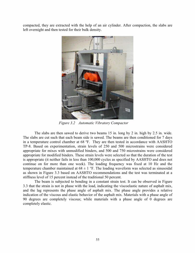
Technical Report Documentation Page 1. Report No. FHWA/TX-06/0-5372-1 2. Government Accession No. 3. Recipient’s Catalog No. 5. Report Date July 2006, Rev. October 2006 4. Title and Subtitle Testing the HB2060 Pads: Equivalent Damage and Fatigue Testing 6. Performing Organization Code 7. Author(s) Vishal Gossain, Karan Kapoor, Jorge A. Prozzi 8. Performing Organization Report No. 0-5372-1 10. Work Unit No. (TRAIS) 9. Performing Organization Name and Address Center for Transportation Research The University of Texas at Austin 3208 Red River, Suite 200 Austin, TX 78705-2650 11. Contract or Grant No. 0-5372 13. Type of Report and Period Covered Technical Report January – August 2005 12. Sponsoring Agency Name and Address Texas Department of Transportation Research and Technology Implementation Office P.O. Box 5080 Austin, TX 78763-5080 14. Sponsoring Agency Code 15. Supplementary Notes Project performed in cooperation with the Texas Department of Transportation and the Federal Highway Administration. 16. Abstract The primary objective of the study was for the Center for Electromechanics, The University of Texas at Austin, to evaluate the Texas Mobile Load Simulator (TxMLS) equipment to recommend the most appropriate rehabilitation options. Within this framework, the research proposed in Project 0-5372 aimed at making the best possible use of the traffic loads that were to be applied as part of the evaluation. A series of secondary objectives included: 1) quantifying the response and performance of a relatively light pavement structure with increased traffic load applications; 2) comparing the performance of the same pavement structure under different axle loads; 3) developing a methodology to estimate the reduction in expected pavement performance as a result of increased axle loads. The contract under which the repairs to the TxMLS and the necessary traffic load tests were to be conducted was discontinued in August 2005. At that time, approximately 40,000 axle load repetitions had been applied to one of the test pads, which did not provide enough data to address the research objectives described above. Therefore, this research report addresses only part of the third objective: the development of a methodology for the estimation of pavement damage under different axle loads and configurations. In addition, results of the asphalt mixture fatigue testing used for the construction of the HB2060 test pads are presented. 17. Key Words Equivalent damage, load equivalency factors, mechanistic design, fatigue testing 18. Distribution Statement No restrictions. This document is available to the public through the National Technical Information Service, Springfield, Virginia 22161; www.ntis.gov. 19. Security Classif. (of report) Unclassified 20. Security Classif. (of this page) Unclassified 21. No. of pages 85 22. Price Form DOT F 1700.7 (8-72) Reproduction of completed page authorized
Transcript
Technical Report Documentation Page
1. Report No. FHWA/TX-06/0-5372-1
2. Government Accession No.
3. Recipient’s Catalog No.
5. Report Date July 2006, Rev. October 2006
4. Title and Subtitle Testing the HB2060 Pads: Equivalent Damage and Fatigue Testing 6. Performing Organization Code
7. Author(s) Vishal Gossain, Karan Kapoor, Jorge A. Prozzi
8. Performing Organization Report No. 0-5372-1
10. Work Unit No. (TRAIS) 9. Performing Organization Name and Address Center for Transportation Research The University of Texas at Austin 3208 Red River, Suite 200 Austin, TX 78705-2650
11. Contract or Grant No. 0-5372
13. Type of Report and Period Covered Technical Report
January – August 2005
12. Sponsoring Agency Name and Address Texas Department of Transportation Research and Technology Implementation Office P.O. Box 5080 Austin, TX 78763-5080
Project performed in cooperation with the Texas Department of Transportation and the Federal Highway Administration.
16. Abstract The primary objective of the study was for the Center for Electromechanics, The University of Texas at Austin, to evaluate the Texas Mobile Load Simulator (TxMLS) equipment to recommend the most appropriate rehabilitation options. Within this framework, the research proposed in Project 0-5372 aimed at making the best possible use of the traffic loads that were to be applied as part of the evaluation. A series of secondary objectives included: 1) quantifying the response and performance of a relatively light pavement structure with increased traffic load applications; 2) comparing the performance of the same pavement structure under different axle loads; 3) developing a methodology to estimate the reduction in expected pavement performance as a result of increased axle loads. The contract under which the repairs to the TxMLS and the necessary traffic load tests were to be conducted was discontinued in August 2005. At that time, approximately 40,000 axle load repetitions had been applied to one of the test pads, which did not provide enough data to address the research objectives described above. Therefore, this research report addresses only part of the third objective: the development of a methodology for the estimation of pavement damage under different axle loads and configurations. In addition, results of the asphalt mixture fatigue testing used for the construction of the HB2060 test pads are presented.
18. Distribution Statement No restrictions. This document is available to the public through the National Technical Information Service, Springfield, Virginia 22161; www.ntis.gov.
19. Security Classif. (of report) Unclassified
20. Security Classif. (of this page) Unclassified
21. No. of pages 85
22. Price
Form DOT F 1700.7 (8-72) Reproduction of completed page authorized
Testing the HB2060 Pads: Equivalent Damage and Fatigue Testing Vishal Gossain Karan Kapoor Jorge A. Prozzi CTR Technical Report: 0-5372-1 Report Date: July 2006, Revised October 2006 Project: 0-5372 Project Title: Testing of HB2060 Pads Sponsoring Agency: Texas Department of Transportation Performing Agency: Center for Transportation Research at The University of Texas at Austin Project performed in cooperation with the Texas Department of Transportation and the Federal Highway Administration.
iv
Center for Transportation Research The University of Texas at Austin 3208 Red River Austin, TX 78705 www.utexas.edu/research/ctr Copyright (c) 2006 Center for Transportation Research The University of Texas at Austin All rights reserved Printed in the United States of America
v
Disclaimers Author's Disclaimer: The contents of this report reflect the views of the authors, who
are responsible for the facts and the accuracy of the data presented herein. The contents do not necessarily reflect the official view or policies of the Federal Highway Administration or the Texas Department of Transportation (TxDOT). This report does not constitute a standard, specification, or regulation.
Patent Disclaimer: There was no invention or discovery conceived or first actually reduced to practice in the course of or under this contract, including any art, method, process, machine manufacture, design or composition of matter, or any new useful improvement thereof, or any variety of plant, which is or may be patentable under the patent laws of the United States of America or any foreign country.
Notice: The United States Government and the State of Texas do not endorse products or manufacturers. If trade or manufacturers' names appear herein, it is solely because they are considered essential to the object of this report.
Engineering Disclaimer NOT INTENDED FOR CONSTRUCTION, BIDDING, OR PERMIT PURPOSES.
Project Engineer: Randy Machemehl
Professional Engineer License State and Number: 41921 P. E. Designation: Jorge A. Prozzi
vi
Acknowledgments The authors express appreciation to German Claros, PC, Research and Technology
Implementation Office, and John Bilyeu, PD, Construction Division, for their assistance during this project.
vii
Table of Contents
1. Introduction............................................................................................................................... 1 1.1 Problem Statement.................................................................................................................1 1.2 General Testing Plan..............................................................................................................3
2. Determination of Load Equivalency Factors ......................................................................... 5 2.1 Mechanistic Design of Pavements.........................................................................................5 2.2 NCHRP 1-37 Project .............................................................................................................8 2.3 Experimental Set-Up and Methodology ..............................................................................13 2.4 Methodology........................................................................................................................18 2.5 Results and Analysis............................................................................................................18 2.6 Equivalent Damage Factors (EDF)......................................................................................33 2.7 Regression Analysis and Applications ................................................................................39
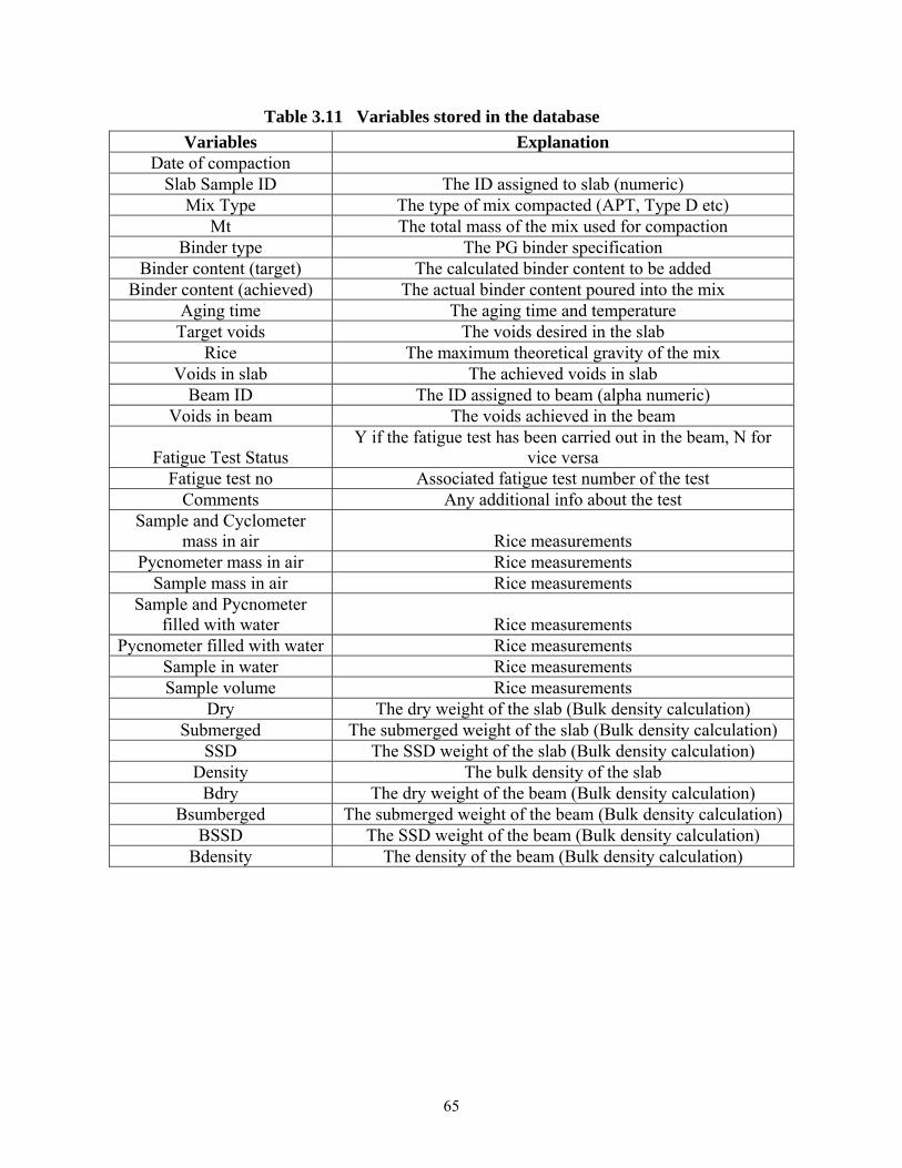
Table 3.11 Variables Stored in the Database ........................................................................... 65
xii
1
1. Introduction
1.1 Problem Statement Texas currently has approximately 17,000 miles of load-zoned roads, the majority of
which are posted at 58,420 lbs. These load limits were set in 1959, just prior to an increase in the allowable gross vehicle weight (GVW) limit to 72,000 lbs. These roads consist primarily of thin pavement structures constructed in the 1940s and 1950s and were originally designed to carry the lighter loads prevailing at that time.
In 1989, the 71st Texas Legislature passed House Bill 2060 (HB 2060), which established a $75-per-county permit to allow truckers to carry legal loads (80,000 lbs plus a 5 percent GVW tolerance = 84,000 lbs) on load-zoned roadways and bridges. Previous research has indicated that the HB 2060 permit fee does not provide sufficient revenue to compensate for the damage resulting from these heavy loads. This conclusion was based on an evaluation of the damage models in the 1986 AASHTO Design Guide, Chapter 4 Low-volume Road Design, and a field study. Although this information was compelling, the HB 2060 permits are still available to truckers that choose to operate on the state’s load-zoned road network.
Accelerated Pavement Testing (APT) has the potential to provide valuable information that, in a relatively short period of time, could visually document the damage caused by heavily loaded trucks to the load-zoned road network. For this reason, in January 2005, researchers with the Center for Transportation Research at The University of Texas at Austin (UT Austin) contracted with the Texas Department of Transportation (TxDOT) to conduct controlled, accelerated pavement tests to evaluate the increased damage to thin pavement structures due to changing axle loads under Research Project 0-5372.
1.1.1 Original Research Objectives It is important to note that the primary objective of the proposed test was for the Center
for Electromechanics at UT Austin to evaluate the Texas Mobile Load Simulator (TxMLS) equipment in order to recommend the most appropriate rehabilitation options. The research proposed as part of TxDOT Project 0-5372 aimed at making the best possible use of the traffic loads that were to be applied as part of the evaluation process. Thus, there were three secondary research objectives, which are described in the following paragraphs.
The first objective of the study was to quantify the response and performance of a relatively light pavement structure with increased traffic load applications under the TxMLS. Because of the lack of an environmental control system, this evaluation was to be conducted at ambient temperature in an outdoor facility at the Pickle Research Center. This objective included the following facets: 1) quantification of the engineering properties of the various pavement layers based on in situ testing by means of falling weight deflectometer (FWD) and rolling dynamic deflectometer (RDD); and 2) determination of the performance of the test sections in terms of cracking and rutting progression and the reduction of the bearing capacity.
The second objective of the series of tests was to compare the performance of the same pavement structure under different axle loads. In turn, this could serve as an experiment to validate currently used approaches to estimate equivalent damage, specifically the effect of axle loads. The following aspects were to be addressed to achieve this objective: 1) evaluation of the
2
response and performance of one pavement structure under four different axle load levels; and 2) performance modeling of the various tests sections and determination of the effects of loads and environment on performance.
The third objective was to develop a methodology to estimate the reduction on expected pavement performance as a result of increased axle loads. The development of this methodology was to be based on the data collected during the project and was going to be used to facilitate the development of guidelines to estimate load equivalency factors for similar pavement structures to those tested under the TxMLS, expanding the test results to a bigger inference space.
The contract that provided for repairs to the TxMLS and the necessary traffic load tests to carry out the tasks outlined in Project 0-5372 was officially discontinued in August 2005. At that time, approximately 40,000 axle load repetitions had been applied to one of the test pads, consequently not providing the data necessary for addressing the research objectives described above. Therefore, this research report addresses only part of the third objective, i.e., the development of a methodology for the estimation of pavement damage under different axle loads and configurations. This methodology was based on the recently developed guide for the “Mechanistic-Empirical Design of New and Rehabilitated Pavement Structures,” hereafter referred to as the M-E Design Guide. This guide was developed under National Cooperative Highway Research Program (NCHRP) Project 1-37A (NCHRP, 2002). In addition, results of the fatigue testing of the asphalt mixture used for the construction of the HB2060 test pads are presented.
1.1.2 Research Approach Accelerated Pavement Testing (APT) of pavements is accepted as an important aid in
decision making for material characterization and pavement design, analysis and performance. This technology is perfectly suited to address the problem stated in this research and to obtain visible short-term results.
The testing originally planned as part of Project 0-5372 was also part of the evaluation and testing of the mechanical capabilities of the TxMLS itself. The research proposed to conduct a series of four accelerated pavement tests using the TxMLS at axle loads representative of a truck operated under the load zone limit and at a suitable range of axle loads representative of legally loaded trucks as well as overloaded trucks. The exact load levels were to be selected depending on the final capabilities of the rehabilitated TxMLS; the four test pads could be tested at 20, 24, 30, and 36 kips, respectively. Although the TxMLS was decommissioned, the test pads still exist and, thus, the possibility still exists for testing the sections should TxDOT supports further pavement research by means of any other APT device. To this effect, the overall research approach is presented herein.
Because of the lack of environmental control, the significant environmental effects on pavement performance, and the variability associated with materials and construction processes of the test pads, it is possible that the performance of the test pad subjected to a higher load level could be better than that of another test pad subjected to a lighter axle load. To minimize this risk, one could test replicate pads; however, the effect of the load would be more significant if the load range were increased. It was, therefore, recommended that instead of using replicates, the four pads should be tested at the load levels indicated earlier.
APT loading should be applied to the various test pads until failure. Failure is primarily defined in terms of rutting and cracking. For this reason, it is imperative that fatigue cracking and surface rutting development should be accurately monitored at different stages of APT
3
trafficking. The loss of bearing capacity of the pavement structure also serves as an alternative failure criterion. The loss of bearing capacity can be determined by the increase in surface deflections as determined by the FWD or estimated from Multi-depth Deflectometer (MDD) measurements. The loss of stiffness can also be monitored by means of the Portable Seismic Pavement Analyzer (P-SPA).
All proposed test sections should be subjected to accelerated traffic to the point where rehabilitation or major maintenance is required. The failure criteria needed to determine this pavement condition are described in the next section and should be consistent for all test sections.
1.1.3 Failure Criteria At a minimum, three main types of failure mechanisms should be evaluated: permanent
deformation, fatigue cracking and loss in bearing capacity (monitored by means of the increase in elastic surface deflection).
Permanent surface deformation: Rutting of the test sections should be determined by the average maximum permanent surface deformation in the wheel paths. Surface rutting should be monitored and recorded periodically so that various terminal criteria, such as 0.5 or 1.0 in., could be evaluated. The mechanical profiler, currently available at TxDOT, should be the primary measuring instrument. The recently developed laser profiler could be evaluated during this stage.
Fatigue cracking: No specific target fatigue failure criteria for cracking of the asphalt surface were set at the beginning of the test. Cracking, however, should be periodically monitored and recorded and a number of criteria should be evaluated. One of these criteria could be 10 percent, 20 percent, and 50 percent of surface cracking as a percentage of length of the wheel path. Under the controlled conditions typical of APT, cracks do not develop and deteriorate as fast as in the field; hence, it is imperative that cracks be detected as soon as they become visible to the naked eye (less than 0.5 mm [0.02 in.]).
Surface Deflection: A potential failure criterion could be based on limiting the percentage increase in surface deflection relative to the surface deflection at the beginning of the test. This criterion is consistent with fatigue testing of asphalt concrete beams in the laboratory, and should be used for reference purposes only and should not effectively determine the failure of the section and the termination of the test.
1.2 General Testing Plan
1.2.1 Original Testing Plan
The study originally proposed involved testing of four test pads at ambient temperatures with the only variable being axle load. The procedure is as follows:
1) Evaluate the bearing capacity of the structure by means of FWD testing and evaluate
the uniformity to determine the specific location of the test pads. Construction information as well as ground penetrating radar (GPR) data can be used to aid in determining the location of the pads.
2) Test the first test pad, Section PRC001, to failure while monitoring and recording its performance on a regular basis with shorter time intervals at the beginning of the test.
4
3) Test the remaining test pads to failure applying accelerated testing to a final condition equivalent to Section PRC001.
1.2.2 Expected Research Benefits The expected benefits of the original research study included the following: 1) Provision of visible physical evidence to document the damage of increased axle
loads to relatively light pavement structures.
2) Evaluation of the current methodology for the determination of load equivalency factor for light pavement structures.
3) Feasibility of mechanistic empirical methods to predict performance using layered elastic analysis and to extrapolate results to similar pavement conditions.
4) Evaluation of the repetitive loading tests to predict performance in the field.
Because of circumstances beyond the control of the research team, only the third point was finally addressed in this research and is presented in this report.
5
2. Determination of Load Equivalency Factors
2.1 Mechanistic Design of Pavements
2.1.1 Pavement Design Approaches To design a pavement structure, guidelines relating to traffic loads, drainage, traffic
volumes, material types, environmental conditions and pavement thickness must be available. Such design guidelines can be based on the results of in situ testing of pavements, which are typically referred to as empirical methods. Alternatively, pavement design could be approached using mechanistic methods. As there are no fully mechanistic methods available to date, another alternative for designing pavements is to use the mechanistic-empirical methodology.
Pavement performance models can also be used in pavement design and analysis. A pavement performance model is an equation that relates variables such as pavement layer thickness, material strength, climatic conditions, applied loads and wheel and axle configurations to performance indicators. These models are developed by correlating theoretical relationships between structural responses and distresses with observed distresses in the field, and are developed from the data collected on the performance of a large number of pavements. Some of the flexible pavement distresses, for which performance equations exist, are rutting, fatigue cracking, thermal cracking and smoothness (ERES, 2002).
2.1.2 The Empirical Approach An empirical approach is based on the results of experiments and involves building
pavement test sections that represent a wide range of road materials and subjecting them to actual or simulated traffic loads. Empirical models are used in this approach. There are three different approaches for conducting these experiments.
Long Term Pavement Performance (LTPP) studies constitute one approach, wherein experiments are carried out over a period of several years on pavements that are subject to normal traffic load (Croney and Croney, 1997). Another approach for conducting these studies is by means of APT, which was used in both the WASHO Road Test carried out in Idaho in 1953-54 and in the AASHO Road Test carried out in Illinois during 1958-1960 (AASHO, 1962). Accelerated pavement testing can be performed using mobile machines, fixed machines or test trucks (ERES, 2002). Although this approach produces results much faster as compared to the LTPP, it should be noted that aging of the pavement materials is not taken into account due to the accelerated traffic that is used in a relatively short period of time (Croney and Croney, 1997). A third approach consists of laboratory testing, wherein tests are conducted for evaluating the pavement materials under laboratory settings (Croney and Croney, 1997). These laboratory testing methods provide information regarding the properties of the pavement system materials and data needed to evaluate existing specifications and design methods. Shift factors, which are the statistical correlations, are used to relate various laboratory testing methods with in situ methods and APT methods.
6
2.1.3 The Mechanistic Approach A mechanistic approach provides a scientific basis for relating the mechanics of structural
behavior to loading. In order to quantify how the load acting on a structure is distributed to its members, certain basic properties of the materials must be known, along with the geometric properties of the structure. Boussinesq (1885) was the first to apply the mechanistic approach to two-layered systems in 1887, followed by Burmister (1943), who in the 1940s developed elastic layered theory to compute stresses, strains and deflections in flexible pavements (Huang, 2004). In the mechanistic approach, mechanistic models are used to estimate pavement responses in terms of stresses, strains and deflections. To date, however, there are no mechanistic models for performance prediction. In reality, mechanistic design approach has not been used for pavement design because of the complex nature of pavement design (ERES, 2002). Currently, empirical information is still needed in order to relate theory to actual pavement performance.
2.1.4 The Mechanistic-Empirical Approach The mechanistic-empirical approach described in this report is based on the methodology
developed in NCHRP Project 1-37A (NCHRP, 2002). Mechanistic models are used to estimate pavement responses, which include stresses, strains, and deflections at critical locations in a pavement structure. Inputs into such models consist of the fundamental mechanical properties of the materials, the applied wheel and axle loads, climatic conditions, and the pavement structure, including the number and thickness of the layers. Typically, stress and strain calculations are made using multi-layered elastic models for flexible pavements and finite elements models for rigid pavements. Dynamic, viscoelastic or plastic models can also be incorporated.
The pavement responses are then used as inputs into the empirical models (or transfer functions) to estimate pavement performance. These empirical models are calibrated using the data obtained from laboratory testing and actual field performance. The empirical models are regression equations that are used to obtain a best fit between actual field performance and predicted distresses. The disadvantage of the regression approach is that the models are conditional to the conditions under which they are developed because they cannot include all the variables that affect the predicted distress. When the values of these variables are similar to those in the original data set, the regression models work well. However, if the models are applied to a different situation, where unaccounted factors change, the predictions are not accurate and the model requires recalibration. The pavement performance, which is obtained from these empirical models, is measured in terms of distresses such as rutting, fatigue cracking, roughness and thermal cracking in the mechanistic-empirical approach. A chart showing the mechanistic-empirical methodology is shown in Figure 2.1.
7
ENVIRONMENT Temperature Moisture
STRUCTURE Thickness
MATERIALS Layers Subgrade
TRAFFIC Vehicle Class Axle loads
MECHANISTIC MODEL Critical stresses and strains
PERFORMANCE PREDICTION Empirical prediction of distresses
FAILURE CRITERIA Performance versus criteria
Requirements satisfied?
FINAL DESIGN
RELIABILITY Des
ign
Itera
tions
Figure 2.1 Mechanistic-Empirical Methodology
2.1.5 Benefits of the Mechanistic-Empirical Approach The mechanistic-empirical design approach, developed under NCHRP Project 1-37A,
provides the designer with the tools to evaluate the effect of variations in materials on pavement performance, including those that are inherent as well as those due to construction procedures. The mechanistic empirical approach provides a rational relationship between construction and materials specification and the design of the pavement structure (ERES, 2002). Some additional benefits of the mechanistic empirical approach are:
1) The effects of differences in climatic conditions on pavement performance can be
included in the design.
2) Better utilization of the available construction materials can be estimated.
8
3) Effects of different vehicle types, traffic speed, axle configurations, and tire types can be incorporated in the design process.
4) Estimates of the consequences of new loading conditions (like the damaging effects of increased loads) can be evaluated.
5) Better pavement diagnostic techniques, such as improved procedures to evaluate premature distress, can be developed.
6) Direct consideration of seasonal and aging effects on materials and designs.
2.2 NCHRP 1-37 Project
2.2.1 The M-E Design Guide The objective of NCHRP Project 1-37A was to develop the M-E Design Guide based on
engineering mechanics principles (NCHRP, 2002). This new method was developed by incorporating many years of existing research into a powerful analytical tool for the design and performance analysis of pavement structures. The M-E Design Guide covers new and rehabilitated pavements, including procedures for life-cycle cost analysis and evaluations of existing pavements. It is based on a calibrated mechanistic design procedure, which integrates all design variables such as material characterization, environmental conditions, traffic analysis, axle load distribution and design reliability. For flexible pavements, the structural models include both a multi-layered linear-elastic program and a finite element program for non-linear analysis. The guide uses a hierarchical approach for incorporating design input variables according to the importance of the project. There are three levels of inputs which can be selected depending on the requirements of the project. Level 1 is based on site-specific measurements and is reserved for the most accurate designs where the consequences of early failure are economically significant. Level 2 is based on regional values or regression equations and is consistent with current version of the AASHTO Design Guide (AASHTO, 1993). Finally, Level 3 design makes use of default values, and hence is the least accurate. The hierarchical approach applies to all aspects of the design guide including traffic, materials and environmental inputs. Once the inputs have been developed in the design guide, structural (performance) analysis is conducted. This is followed by the evaluation of technically viable alternatives (McGhee, 1999).
2.2.2 Design Inputs
The inputs of pavement design vary with the type of structure being designed. The design inputs include pavement structure, climatic conditions, pavement materials, soil conditions and traffic loading. The design inputs can be broadly classified into two categories (ERES, 2002):
1) Site Variables: those over which the pavement designer has no control, such as
climate, soil conditions, and traffic, and have to be accommodated in the design process.
2) Design Variables: those over which the designer has control and can change in order to accommodate the design criteria, for example, the number of pavement layers, type of pavement materials, and layer thicknesses.
9
2.2.3 Number of Repetitions In the M-E Design Guide, performance is expressed as a function of time or cumulative
number of all trucks. Several performance indicators are considered, such as total rutting, rutting of individual layers, surface-down fatigue cracking or longitudinal cracking, bottom-up fatigue cracking or alligator cracking, thermal cracking, and fatigue fracture in a chemically stabilized base layer. The number is obtained for repetitions of all axles of the traffic stream necessary to reach pre-established levels of the failure. For the purpose of this study, these criteria are 0.5 in. of surface rutting, and 10 percent fatigue cracking as a percentage of length of the wheel path. The number of axle load repetitions to reach the failure criteria is referred to as pavement life. Most of the previous pavement design and analysis methods express performance based on the number of Equivalent Single Axle Loads (ESALs) to failure.
2.2.4 Failure Mechanisms The failure mechanisms used to study pavement performance are described in the
following paragraphs.
2.2.4.1 Fatigue Cracking Fatigue cracking is one mode of load associated structural failure. There are two forms of
fatigue cracking considered in the M-E Design Guide: top-down and bottom-up. Bottom-up fatigue cracking is governed by the maximum horizontal tensile strain at the bottom of the hot mix asphalt. Bottom-up initiates at the bottom and propagates upwards. It is widely accepted as a distress mode that predominantly occurs in the thicker asphalt layers (4 in. or more). Top-down initiates at the surface of the pavement and propagates downwards.
For the purpose of this research, the failure criterion for pavement in terms of fatigue cracking is selected as 10 percent of fatigue cracking. The fatigue life is represented in terms of load repetitions for the pavement to reach failure in terms of fatigue cracking (Huang, 2004). The ratio of the actual number of load repetitions to the allowable number of load repetitions before failure is a factor known as damage ratio, which is computed for each load in all seasons and is accumulated over the life of the pavement. Fatigue damage occurs in two phases, the first being crack initiation, followed by crack propagation (Ayres and Witczak, 1998). The number of repetitions for crack initiation is the number of repetitions of the load needed for a small visible crack to originate. The fatigue equation used in the M-E Design Guide is the one proposed by The Asphalt Institute in 1982 and is given as Equation 2.1 (Asphalt Institute, 1982). The parameters used in this equation are determined in the laboratory using the bending beam fatigue test at constant stress or constant strain. However, these parameters need to be adjusted in order to represent the actual field conditions.
3322 11**00432.0 11
ββ
εβ
kk
tf E
kCN ⎟⎠⎞
⎜⎝⎛
⎟⎟⎠
⎞⎜⎜⎝
⎛=
(2.1) Where,
MC 10=
⎟⎟⎠
⎞⎜⎜⎝
⎛−
+= 69.084.4
ba
b
VVV
M
fN = number of repetitions for fatigue cracking,
10
tε = maximum tensile strain at the bottom of asphalt layer, E = dynamic modulus of the asphalt layer,
aV = percentage air voids, bV = percentage volume of effective bitumen, 1k = -0.00432 2k = 3.9492 3k = 1.281, and β1, β2, β3 = calibration constants.
The next phase is the crack propagation phase, in which the number of repetitions for the
pavement to reach failure after crack initiation is obtained. For the purpose of this study, the failure criterion was 10 percent cracking.
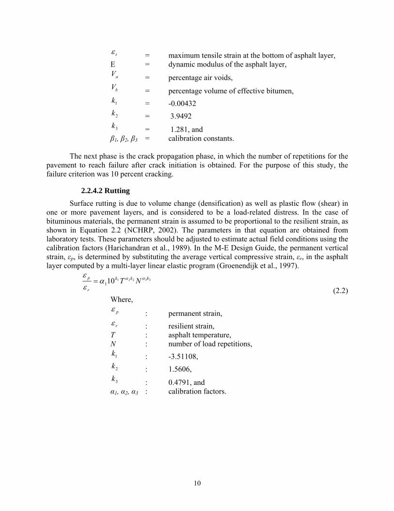
2.2.4.2 Rutting Surface rutting is due to volume change (densification) as well as plastic flow (shear) in
one or more pavement layers, and is considered to be a load-related distress. In the case of bituminous materials, the permanent strain is assumed to be proportional to the resilient strain, as shown in Equation 2.2 (NCHRP, 2002). The parameters in that equation are obtained from laboratory tests. These parameters should be adjusted to estimate actual field conditions using the calibration factors (Harichandran et al., 1989). In the M-E Design Guide, the permanent vertical strain, εp, is determined by substituting the average vertical compressive strain, εr, in the asphalt layer computed by a multi-layer linear elastic program (Groenendijk et al., 1997).
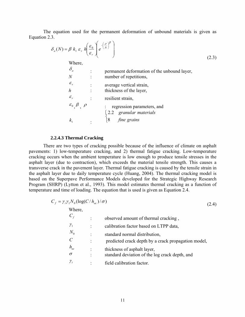
2.2.4.3 Thermal Cracking There are two types of cracking possible because of the influence of climate on asphalt
pavements: 1) low-temperature cracking, and 2) thermal fatigue cracking. Low-temperature cracking occurs when the ambient temperature is low enough to produce tensile stresses in the asphalt layer (due to contraction), which exceeds the material tensile strength. This causes a transverse crack in the pavement layer. Thermal fatigue cracking is caused by the tensile strain in the asphalt layer due to daily temperature cycle (Huang, 2004). The thermal cracking model is based on the Superpave Performance Models developed for the Strategic Highway Research Program (SHRP) (Lytton et al., 1993). This model estimates thermal cracking as a function of temperature and time of loading. The equation that is used is given as Equation 2.4.
)/)/(log(01 σγγ actf hCNC = (2.4)
Where, fC : observed amount of thermal cracking ,
1γ : calibration factor based on LTPP data, 0N : standard normal distribution,
C : predicted crack depth by a crack propagation model, ach : thickness of asphalt layer,
σ : standard deviation of the log crack depth, and tγ : field calibration factor.
12
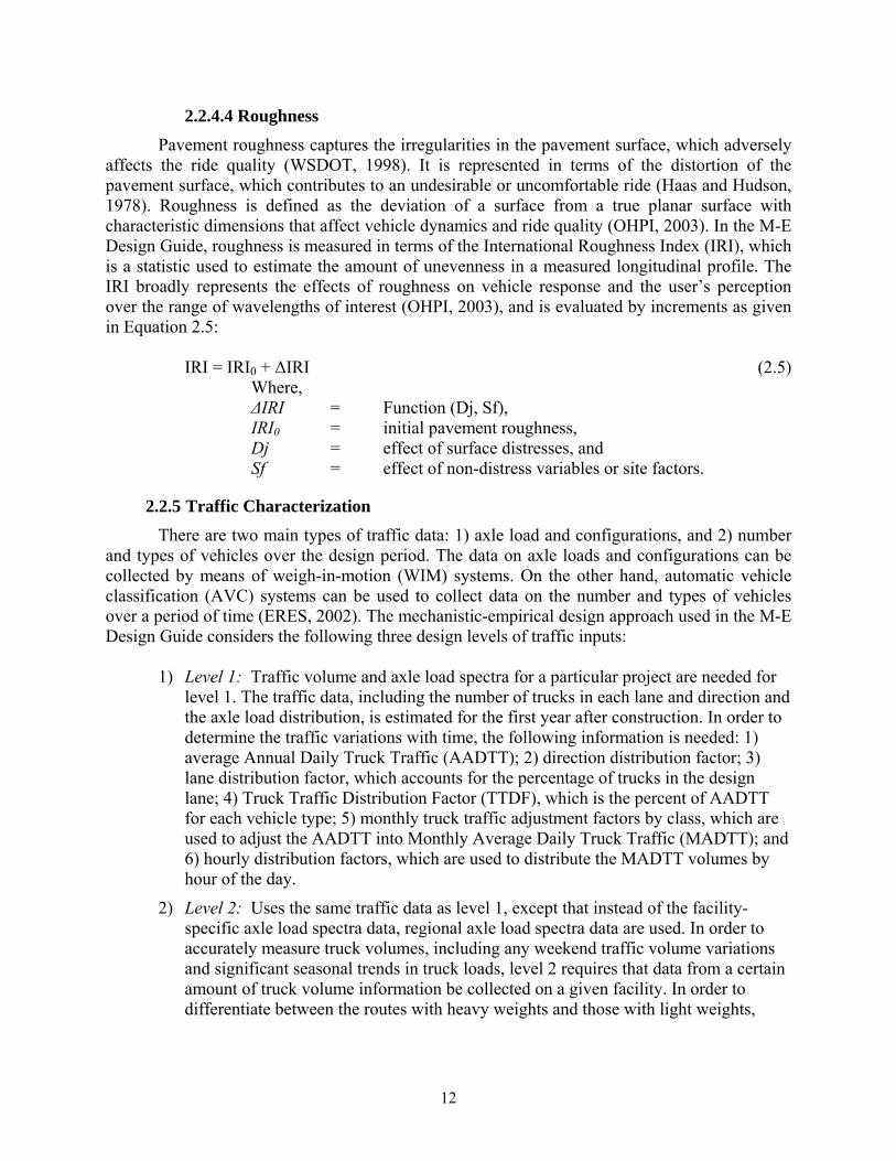
2.2.4.4 Roughness
Pavement roughness captures the irregularities in the pavement surface, which adversely affects the ride quality (WSDOT, 1998). It is represented in terms of the distortion of the pavement surface, which contributes to an undesirable or uncomfortable ride (Haas and Hudson, 1978). Roughness is defined as the deviation of a surface from a true planar surface with characteristic dimensions that affect vehicle dynamics and ride quality (OHPI, 2003). In the M-E Design Guide, roughness is measured in terms of the International Roughness Index (IRI), which is a statistic used to estimate the amount of unevenness in a measured longitudinal profile. The IRI broadly represents the effects of roughness on vehicle response and the user’s perception over the range of wavelengths of interest (OHPI, 2003), and is evaluated by increments as given in Equation 2.5:
IRI = IRI0 + ΔIRI (2.5)
Where, ΔIRI = Function (Dj, Sf), IRI0 = initial pavement roughness, Dj = effect of surface distresses, and Sf = effect of non-distress variables or site factors.
2.2.5 Traffic Characterization There are two main types of traffic data: 1) axle load and configurations, and 2) number
and types of vehicles over the design period. The data on axle loads and configurations can be collected by means of weigh-in-motion (WIM) systems. On the other hand, automatic vehicle classification (AVC) systems can be used to collect data on the number and types of vehicles over a period of time (ERES, 2002). The mechanistic-empirical design approach used in the M-E Design Guide considers the following three design levels of traffic inputs:
1) Level 1: Traffic volume and axle load spectra for a particular project are needed for level 1. The traffic data, including the number of trucks in each lane and direction and the axle load distribution, is estimated for the first year after construction. In order to determine the traffic variations with time, the following information is needed: 1) average Annual Daily Truck Traffic (AADTT); 2) direction distribution factor; 3) lane distribution factor, which accounts for the percentage of trucks in the design lane; 4) Truck Traffic Distribution Factor (TTDF), which is the percent of AADTT for each vehicle type; 5) monthly truck traffic adjustment factors by class, which are used to adjust the AADTT into Monthly Average Daily Truck Traffic (MADTT); and 6) hourly distribution factors, which are used to distribute the MADTT volumes by hour of the day.
2) Level 2: Uses the same traffic data as level 1, except that instead of the facility-specific axle load spectra data, regional axle load spectra data are used. In order to accurately measure truck volumes, including any weekend traffic volume variations and significant seasonal trends in truck loads, level 2 requires that data from a certain amount of truck volume information be collected on a given facility. In order to differentiate between the routes with heavy weights and those with light weights,
13
vehicle weights are taken from vehicle weight summaries, which are maintained by each state (ERES, 2002).
3) Level 3: In case the designer has only the AADTT and the percentage distribution of the trucks for the particular roadway section under study, then level 3 traffic data is used by employing regional or state default classification and axle load spectra data (ERES, 2002).
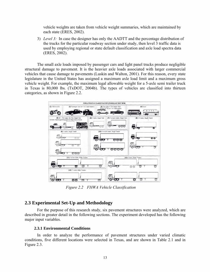
The small axle loads imposed by passenger cars and light panel trucks produce negligible
structural damage to pavement. It is the heavier axle loads associated with larger commercial vehicles that cause damage to pavements (Luskin and Walton, 2001). For this reason, every state legislature in the United States has assigned a maximum axle load limit and a maximum gross vehicle weight. For example, the maximum legal allowable weight for a 5-axle semi trailer truck in Texas is 80,000 lbs. (TxDOT, 2004b). The types of vehicles are classified into thirteen categories, as shown in Figure 2.2.
Figure 2.2 FHWA Vehicle Classification
2.3 Experimental Set-Up and Methodology For the purpose of this research study, six pavement structures were analyzed, which are
described in greater detail in the following sections. The experiment developed has the following major input variables.
2.3.1 Environmental Conditions In order to analyze the performance of pavement structures under varied climatic
conditions, five different locations were selected in Texas, and are shown in Table 2.1 and in Figure 2.3.
14
Table 2.1 Test Locations
Code Station Latitude (deg. min)
Longitude (deg. min)
Elevation (ft)
AUS Austin City 30.19 -97.46 648 AMA Amarillo 35.13 -101.43 3586 DFW Dallas Fort Worth 32.54 -97.02 559 ELP El Paso 31.49 -106.23 3942
The rationale behind selecting these locations was to represent different geographical locations and varying climatic conditions existing in Texas. Following are the locations and the types of weather conditions prevailing at these stations:
1) Amarillo (AMA, dry/cold): represents the Texas Panhandle region, having dry cold
weather, and high elevation. Amarillo has a maximum temperature of 92°F (34°C) in
15
summer and a minimum temperature of 22°F (-4°C) in winter, with annual rainfall of 19.5 in. (495.3 mm).
2) Austin (AUS, mixed): represents Central Texas, having moderate temperatures, with a maximum of 98°F (37°C) in summer and minimum of 42°F (7°C) in winter, and annual rainfall of 32.5 in. (825.5 mm).
3) Dallas Fort Worth (DFW, wet/cold): represents wet and cold weather in the state of Texas. Dallas has a maximum temperature of 100°F (37°C) in summer and a minimum of 33°F (0°C) in winter with an annual rainfall of 32 in. (812.8 mm).
4) El Paso (ELP, dry/warm): represents southwest Texas, at the border of Mexico, with dry warm weather. Temperatures in El Paso vary from 97°F (37°C) to 64°F (18°C) in summer and from 56°F (14°C) to 29°F (-1°C) in winter, with an annual rainfall of 8.65 in. (219.7 mm).
5) Houston (IAH, wet/warm): lies along the Gulf of Mexico, representing hot and humid weather. Houston has a maximum temperature of 90°F (32°F) in summer and a minimum temperature of 40°F (4°F) in winter, with annual precipitation of 46.07 in. (1170.2 mm).
2.3.2 Pavement Structures The six pavement structures selected for experimentation consisted of four layers. The
same materials were used for all the structures. The material properties were selected to be consistent with the AASHO Road Test, as the designs are based on the current AASHTO Design Guide (AASHTO, 1993). The main properties are:
1) Asphalt Surface: the top layer, which consists of dense-graded crushed dolomitic
limestone aggregate, ¾-in. maximum size, and natural sand with about 5.4 percent of 85-100 penetration grade paving asphalt (AASHO, 1962).
2) A-1-b base: consists of a gravel base of crushed dolomitic limestone; 1½-in.maximum size, and a maximum dry density of 140 pcf (AASHO, 1962).
3) A-2-4 subbase: comprised of sand gravel material, containing small amounts of fine sand and friable fine grained soil; 1-in. maximum size, and a maximum dry density of 138 pcf (AASHO, 1962).
4) A-6 subgrade: comprised of a plastic clay soil having 75.5 percent passing the 0.075-mm (No. 200) sieve, and 96.6 percent passing the 4.75-mm (No. 4) sieve. The maximum dry unit weight of the material was 116.4 pcf (AASHO, 1962).
The particle size distribution of the chosen materials is shown in Figure 2.4, and their main properties are as shown in Table 2.2. The materials were selected consistent with the AASHO Road Test experiment so the pavement performance could be evaluated and compared between pavement designed by the empirical method (AASHTO, 1993) and that designed by the M-E Design Guide (NCHRP, 2002). The only exception to the selection method was the subgrade layer, whose resilient modulus was selected to be more consistent with Texas conditions.
16
0
20
40
60
80
100
120
0.001 0.01 0.1 1 10Particle size (inches)
% F
iner
AsphaltSubbaseBase
Figure 2.4 Gradation Curve for Different Materials (AASHO, 1962)
Table 2.2 Pavement Layers
Layer Material a Modulus(psi) Surface Dense Asphalt 0.44
Different layer thicknesses were then selected for these structures and are shown in Table
2.3. Using the layer strength coefficients (a value) given in Table 2.2 and the layer thicknesses from Table 2.3, the structural numbers for the six structures were calculated, using Equation 2.6 and are also given in Table 2.3.
Table 2.3 Layer Thicknesses
Structures Layer #1 #2 #3 #4 #5 #6
Surface 2 2 4 4 6 6 Base 6 9 6 9 6 9
Subbase 4 8 8 8 8 12
Subgrade Semi-infinite
Semi-infinite
Semi-infinite
Semi-infinite
Semi-infinite
Semi-infinite
SN 2.16 3.02 3.48 3.9 4.36 5.22
17
332211 DaDaDaSN ++= (2.6) Where, SN : Structural Number of the pavement, a1 : layer coefficient for surface, a2 : layer coefficient for base, a3 : layer coefficient for subbase, D1 : asphalt surface thickness, D2 : base thickness, and D3 : subbase thickness.
2.3.3 Traffic Volume Once the pavement structures were designed and their structural numbers were
calculated, the expected traffic volumes were calculated using the empirical design Equation 2.7 (AASHTO, 1993). This equation was developed based primarily on the results of the AASHO Road Test. It expresses the expected design traffic (in ESALs) as a function of the structural number (SN), the allowable change in pavement serviceability index (∆PSI), the resilient modulus of the subgrade (MR), and the reliability.
( ) ( )[ ]( )
07.8log32.21/10944.0
5.12.4/log20.01log36.9log 19.5018
−+++−Δ
+−++=
R
Rt
MSN
PSISNSZW
(2.7) Where,
18tW : number of equivalent 18 kips single axle load applications, PSIΔ : change in Pavement Serviceability Index (p0-pf), RZ : normal deviate for a given reliability R, and
S0 : standard deviation. For comparative purposes, 50 percent reliability was used in this study, however, any
other level of reliability could be used, including different reliability levels for each structure because high-volume roads are usually designed to higher standards. At 50 percent reliability, ZR value is 0, and a p0 value of 4.4 and pf value of 2.5 are used, which gives a ΔPSI of 1.9. The expected ESALs obtained for the six structures are given in Table 2.4. Using these design ESALs, AADTT values are calculated assuming a design life of 20 years and no traffic growth.
The axle load spectrum is the distribution of axle loads for single, tandem, tridem, and quad axles as a percentage of the total number of single, tandem, tridem, and quad axles, respectively. For the purpose of this study, all the structures are simulated only under single and tandem axles. The axle loads used are given in Table 2.5.
Table 2.5 Axle Loads Used in this Research Single (kips) Tandem (kips)
12 26 15 30 18 34 21 38 24 42
2.4 Methodology Empirical traffic volumes were obtained based on the AASHTO 1993 Design Guide, as
given in Table 2.4. Using these empirical values, the structures were analyzed for failure in terms of rutting and fatigue cracking performance. Upon analysis of the structures, it was observed that pavement deterioration was slowest in AMA, compared to the other four locations. Hence, it was decided to use AMA as the base location, and the smallest axle load of 12 kips single axle was used to determine the “mechanistic” traffic for the six structures. It should be noted that these mechanistic-based values are expressed in single axles rather than actual trucks.
The traffic volume to reach failure was compared with the empirical traffic volumes given in Table 2.4. If the failure was not obtained as predicted, the traffic volumes were adjusted accordingly so that failure was obtained at the same predicted time by the empirical design. In the next part of the study, pavement life was evaluated relative to the life under the standard 18 kips single axle load. Since the load repetitions indicate the pavement life for different axle loads, the pavement lives are different under different axle loads making it difficult to determine generalized trends. Hence, this analysis was carried out by applying the Equivalent Damage Factor (EDF) concept developed in South Africa (Prozzi and de Beer, 1997).
2.5 Results and Analysis
2.5.1 Results
The six pavement structures were analyzed for each of the five locations. Hence, a total of thirty different conditions were evaluated under five different single axle loads and five different tandem axle loads. Pavement performance was evaluated in terms of rutting and fatigue cracking. Other failure mechanisms that were evaluated but not considered for analysis were thermal cracking and roughness. The reason they were not selected was that unrealistic performance predictions were obtained, which could be attributed to the lack of local calibration.
A comparison of ESAL values based on empirical values and mechanistic-empirical values for rutting and fatigue for AMA 18 kips single axle load is shown in Table 2.6, as an example. The mechanistic-empirical approach estimated longer pavement lives for structures 1 and 2 as compared to the empirical design values based on AASHTO 1993. For structure 3, the
19
mechanistic-empirical and empirical values are comparable. On the other hand, for structures 4, 5, and 6, the mechanistic-based analysis estimates longer pavement lives in terms of fatigue, and shorter pavement lives in terms of rutting, as compared to the empirical based design lives. The difference between empirical and mechanistic-empirical values can be explained by several reasons, one being that the failure criterion in AASHTO 1993 is based on riding quality in terms of PSI, and the failure criteria used in the mechanistic-empirical approach are in terms of rutting and fatigue cracking. As the structural number increases, the empirical pavement life increases, whereas the mechanistic-empirical pavement life initially increases and then decreases.
Table 2.6 Empirical and Mechanistic-Empirical Design Lives Empirical
2.5.2 Rutting Figure 2.5 represents rutting as a function of the structural number of the various
structures, using 18 kips standard single axle load. It can be observed that as the structural number is increased, the rutting life decreases, and after a certain critical value of the structural number, as the structural number is further increased, the rutting life starts increasing. Hence, the pavement performance deteriorates initially as the structural number is increased; then with further increase in structural number, the pavement performance improves after the critical value of the structural number. This phenomenon of critical thickness has been observed for fatigue cracking life but never before for surface rutting.
20
0.0
1.0
2.0
3.0
4.0
5.0
6.0
7.0
2 3 4 5 6
Structural Numbers
Rut
ting
Life
for 1
8 ki
ps S
ingl
e A
xle
Load
(in m
illio
ns) AMA
AUSDFWELPIAH
Figure 2.5 Rutting Life for 18 kips Standard Single Axle Load
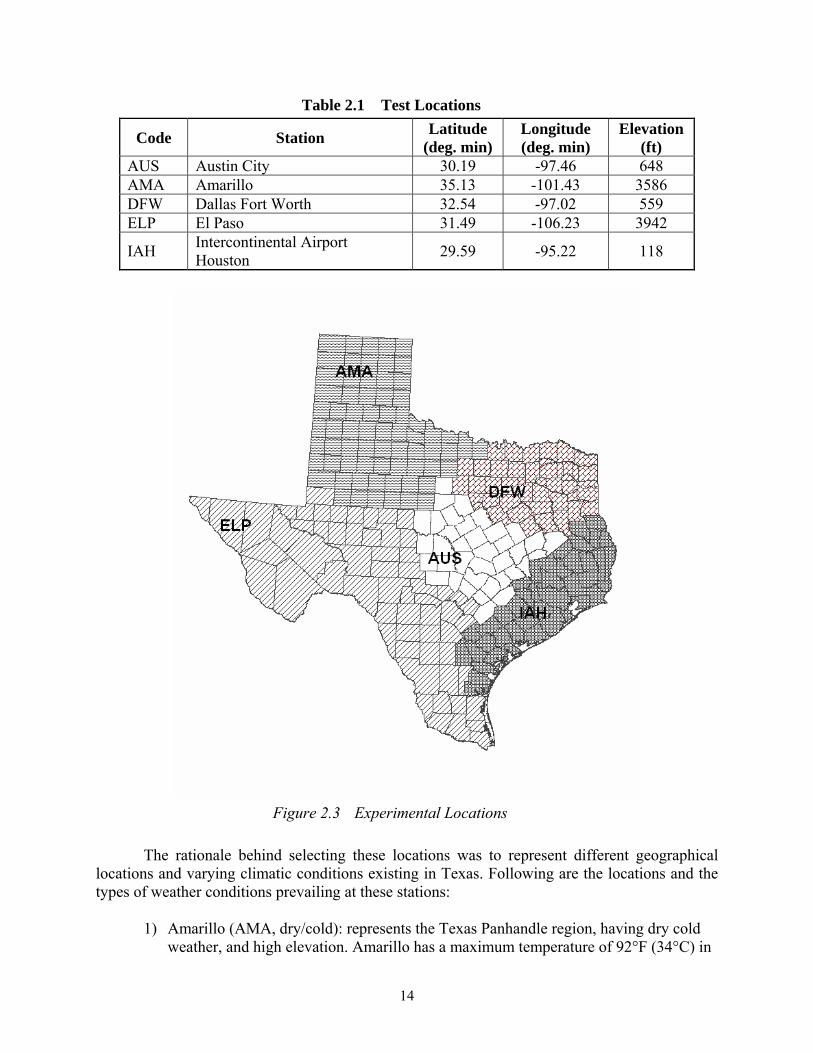
The plots of the rutting life for single axle loads for the six structures at each of the locations are also shown in figures 2.6 to 2.11. These figures show that as the axle loads are increased from 12,000 lbs to 24,000 lbs, the number of repetitions of the axle loads required for the pavements to reach 0.5” rutting is reduced from 12,300,000 (AMA- S2) to 1,145,000 (ELP- S2), implying increased deterioration in the pavements.
Also, while everything else is kept constant, amongst the five stations, AMA requires the highest number of repetitions to reach 0.5” surface rutting for all the six structures, indicating slow deterioration in terms of rutting in Amarillo. Also, AUS and ELP can be seen as the locations reaching 0.5” of rutting with the least number of axle repetitions compared to the other locations. Hence, out of these five stations, the fastest pavement deterioration in terms of rutting takes place in AUS and ELP, which could be attributed to the warmer climates in those areas. The slow pavement deterioration in AMA can be attributed to the colder weather conditions in that area.
Figure 2.11 Rutting Life of Structure 6 for Single Axle Loads
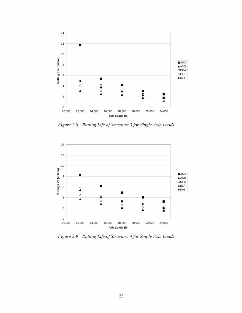
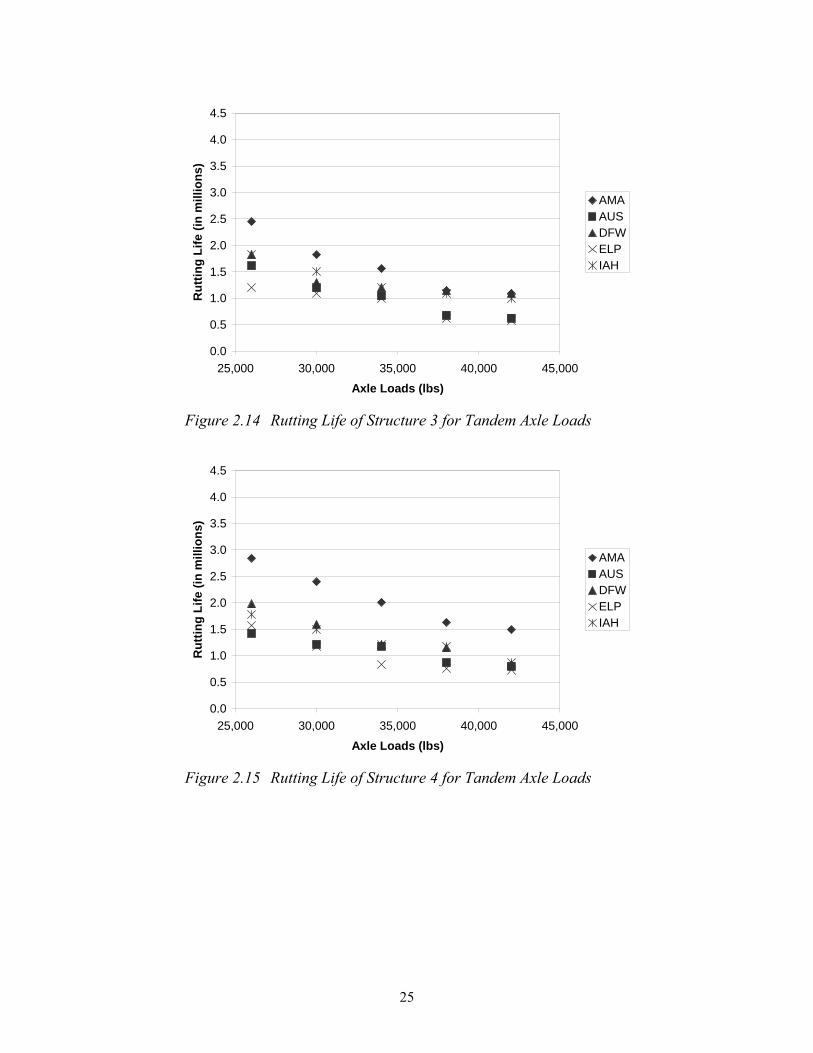
The plots of the rutting life for tandem axle loads for the six structures at each of the locations are shown in figures 2.12 to 2.17. Similar trends are observed from the results of rutting life for tandem axles. It is again observed that as the axle loads are increased from 26,000 lbs to 42,000 lbs, the number of axle load repetitions required for the pavements to reach 0.5” rutting is reduced from 4,200,000 (AMA- S2) to 520,000 (ELP- S1), implying increased pavement deterioration.
Also, while everything else is kept constant, amongst the five stations, AMA requires the largest number of repetitions to reach 0.5” of rutting, for all the six structures. Also, AUS and
24
ELP can be seen as the areas reaching 0.5” of rutting with the least number of repetitions compared to the other locations.
0.0
0.5
1.0
1.5
2.0
2.5
3.0
3.5
4.0
4.5
25,000 30,000 35,000 40,000 45,000
Axle Loads (lbs)
Rut
ting
Life
(in
mill
ions
)
AMAAUSDFWELPIAH
Figure 2.12 Rutting Life of Structure 1 for Tandem Axle Loads
0.0
0.5
1.0
1.5
2.0
2.5
3.0
3.5
4.0
4.5
25,000 30,000 35,000 40,000 45,000
Axle Loads (lbs)
Rut
ting
Life
(in
mill
ions
)
AMAAUSDFWELPIAH
Figure 2.13 Rutting Life of Structure 2 for Tandem Axle Loads
25
0.0
0.5
1.0
1.5
2.0
2.5
3.0
3.5
4.0
4.5
25,000 30,000 35,000 40,000 45,000
Axle Loads (lbs)
Rut
ting
Life
(in
mill
ions
)AMAAUSDFWELPIAH
Figure 2.14 Rutting Life of Structure 3 for Tandem Axle Loads
0.0
0.5
1.0
1.5
2.0
2.5
3.0
3.5
4.0
4.5
25,000 30,000 35,000 40,000 45,000
Axle Loads (lbs)
Rut
ting
Life
(in
mill
ions
)
AMAAUSDFWELPIAH
Figure 2.15 Rutting Life of Structure 4 for Tandem Axle Loads
26
0.0
0.5
1.0
1.5
2.0
2.5
3.0
3.5
4.0
4.5
25,000 30,000 35,000 40,000 45,000
Axle Loads (lbs)
Rut
ting
Life
(in
mill
ions
)AMAAUSDFWELPIAH
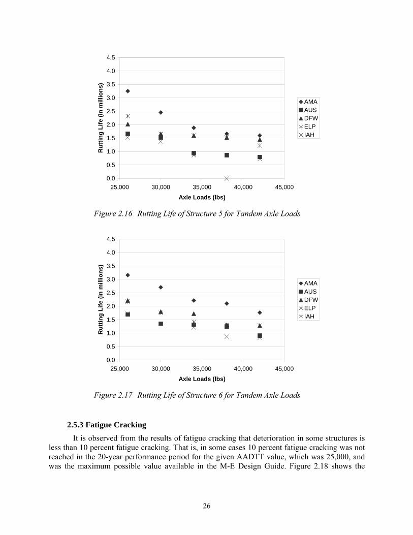
Figure 2.16 Rutting Life of Structure 5 for Tandem Axle Loads
0.0
0.5
1.0
1.5
2.0
2.5
3.0
3.5
4.0
4.5
25,000 30,000 35,000 40,000 45,000
Axle Loads (lbs)
Rut
ting
Life
(in
mill
ions
)
AMAAUSDFWELPIAH
Figure 2.17 Rutting Life of Structure 6 for Tandem Axle Loads
2.5.3 Fatigue Cracking It is observed from the results of fatigue cracking that deterioration in some structures is
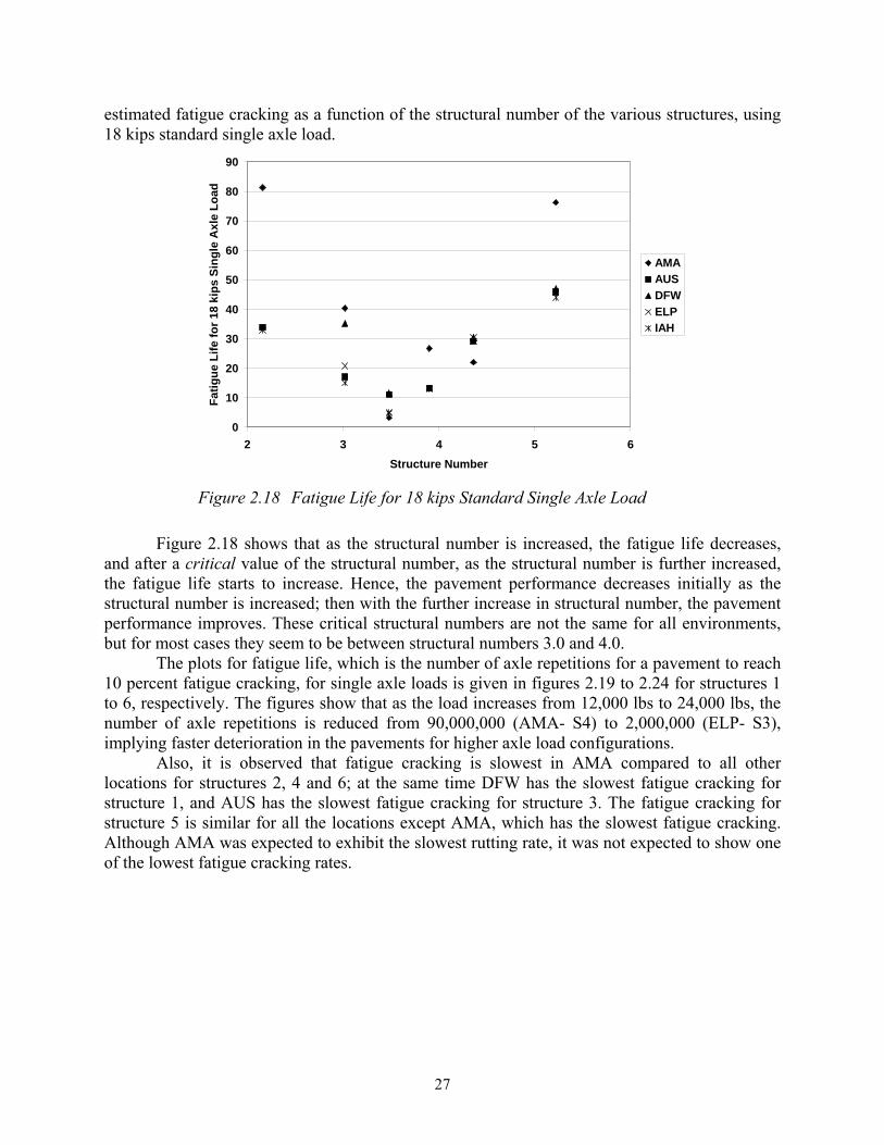
less than 10 percent fatigue cracking. That is, in some cases 10 percent fatigue cracking was not reached in the 20-year performance period for the given AADTT value, which was 25,000, and was the maximum possible value available in the M-E Design Guide. Figure 2.18 shows the
27
estimated fatigue cracking as a function of the structural number of the various structures, using 18 kips standard single axle load.
0
10
20
30
40
50
60
70
80
90
2 3 4 5 6Structure Number
Fatig
ue L
ife fo
r 18
kips
Sin
gle
Axl
e Lo
ad
AMAAUSDFWELPIAH
Figure 2.18 Fatigue Life for 18 kips Standard Single Axle Load
Figure 2.18 shows that as the structural number is increased, the fatigue life decreases, and after a critical value of the structural number, as the structural number is further increased, the fatigue life starts to increase. Hence, the pavement performance decreases initially as the structural number is increased; then with the further increase in structural number, the pavement performance improves. These critical structural numbers are not the same for all environments, but for most cases they seem to be between structural numbers 3.0 and 4.0.
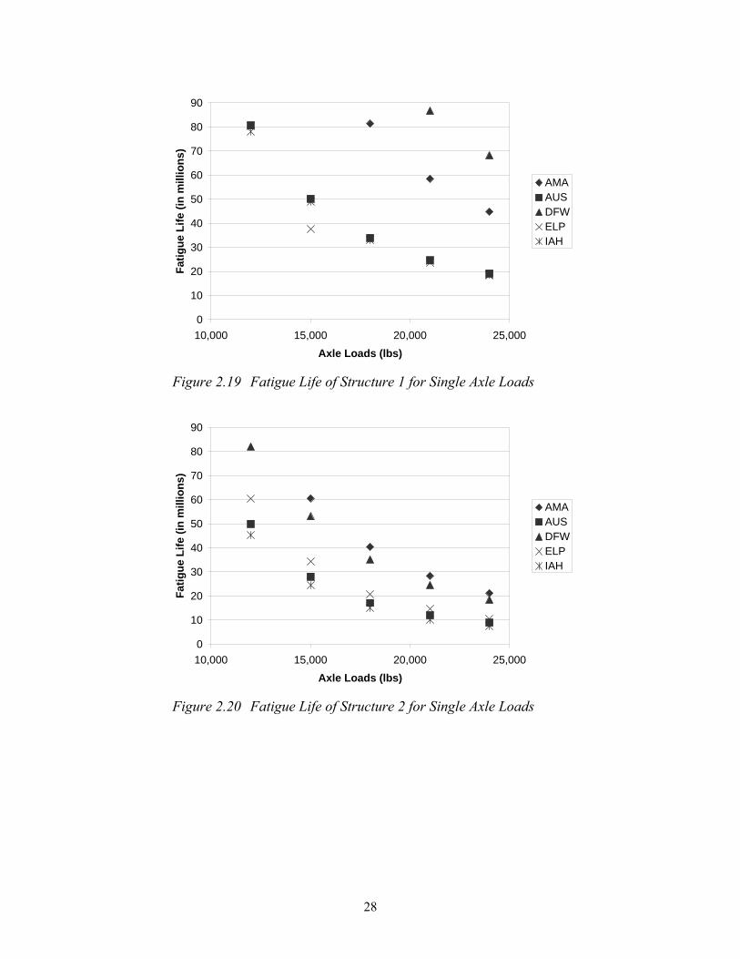
The plots for fatigue life, which is the number of axle repetitions for a pavement to reach 10 percent fatigue cracking, for single axle loads is given in figures 2.19 to 2.24 for structures 1 to 6, respectively. The figures show that as the load increases from 12,000 lbs to 24,000 lbs, the number of axle repetitions is reduced from 90,000,000 (AMA- S4) to 2,000,000 (ELP- S3), implying faster deterioration in the pavements for higher axle load configurations.
Also, it is observed that fatigue cracking is slowest in AMA compared to all other locations for structures 2, 4 and 6; at the same time DFW has the slowest fatigue cracking for structure 1, and AUS has the slowest fatigue cracking for structure 3. The fatigue cracking for structure 5 is similar for all the locations except AMA, which has the slowest fatigue cracking. Although AMA was expected to exhibit the slowest rutting rate, it was not expected to show one of the lowest fatigue cracking rates.
28
0
10
20
30
40
50
60
70
80
90
10,000 15,000 20,000 25,000Axle Loads (lbs)
Fatig
ue L
ife (i
n m
illio
ns)
AMAAUSDFWELPIAH
Figure 2.19 Fatigue Life of Structure 1 for Single Axle Loads
0
10
20
30
40
50
60
70
80
90
10,000 15,000 20,000 25,000Axle Loads (lbs)
Fatig
ue L
ife (i
n m
illio
ns)
AMAAUSDFWELPIAH
Figure 2.20 Fatigue Life of Structure 2 for Single Axle Loads
29
0
10
20
30
40
50
60
70
80
90
10,000 15,000 20,000 25,000Axle Loads (lbs)
Fatig
ue L
ife (i
n m
illio
ns)
AMAAUSDFWELPIAH
Figure 2.21 Fatigue Life of Structure 3 for Single Axle Loads
0
10
20
30
40
50
60
70
80
90
10,000 15,000 20,000 25,000Axle Loads (lbs)
Fatig
ue L
ife (i
n m
illio
ns)
AMAAUSDFWELPIAH
Figure 2.22 Fatigue Life of Structure 4 for Single Axle Loads
30
0
10
20
30
40
50
60
70
80
90
10,000 15,000 20,000 25,000Axle Loads (lbs)
Fatig
ue L
ife (i
n m
illio
ns)
AMAAUSDFWELPIAH
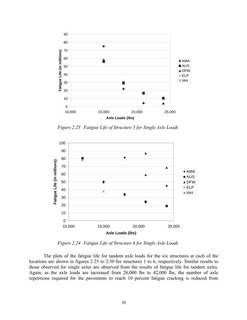
Figure 2.23 Fatigue Life of Structure 5 for Single Axle Loads
0
10
20
30
40
50
60
70
80
90
100
10,000 15,000 20,000 25,000
Axle Loads (lbs)
Fatig
ue L
ife (i
n m
illio
ns)
AMAAUSDFWELPIAH
Figure 2.24 Fatigue Life of Structure 6 for Single Axle Loads
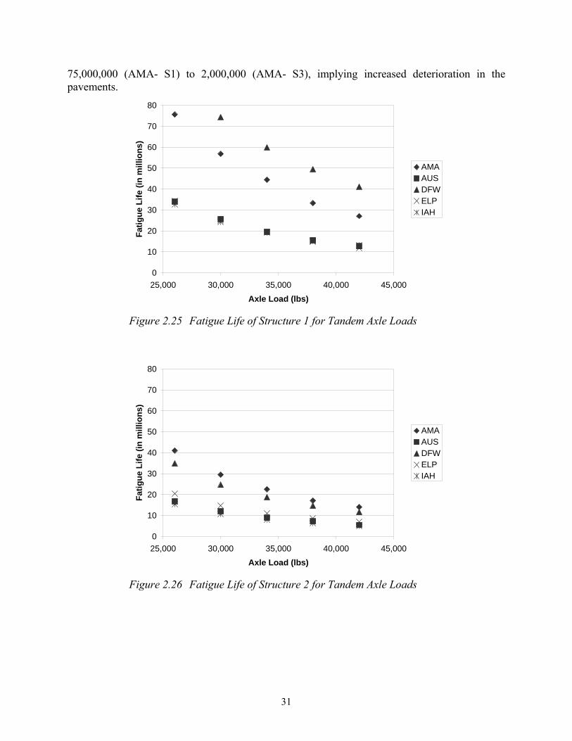
The plots of the fatigue life for tandem axle loads for the six structures at each of the locations are shown in figures 2.25 to 2.30 for structures 1 to 6, respectively. Similar results to those observed for single axles are observed from the results of fatigue life for tandem axles. Again, as the axle loads are increased from 26,000 lbs to 42,000 lbs, the number of axle repetitions required for the pavements to reach 10 percent fatigue cracking is reduced from
31
75,000,000 (AMA- S1) to 2,000,000 (AMA- S3), implying increased deterioration in the pavements.
0
10
20
30
40
50
60
70
80
25,000 30,000 35,000 40,000 45,000Axle Load (lbs)
Fatig
ue L
ife (i
n m
illio
ns)
AMAAUSDFWELPIAH
Figure 2.25 Fatigue Life of Structure 1 for Tandem Axle Loads
0
10
20
30
40
50
60
70
80
25,000 30,000 35,000 40,000 45,000Axle Load (lbs)
Fatig
ue L
ife (i
n m
illio
ns)
AMAAUSDFWELPIAH
Figure 2.26 Fatigue Life of Structure 2 for Tandem Axle Loads
32
0
10
20
30
40
50
60
70
80
25,000 30,000 35,000 40,000 45,000Axle Load (lbs)
Fatig
ue L
ife (i
n m
illio
ns)
AMAAUSELPIAH
Figure 2.27 Fatigue Life of Structure 3 for Tandem Axle Loads
0
10
20
30
40
50
60
70
80
25,000 30,000 35,000 40,000 45,000Axle Load (lbs)
Fatig
ue L
ife (i
n m
illio
ns)
AMAAUSDFWELPIAH
Figure 2.28 Fatigue Life of Structure 4 for Tandem Axle Loads
33
0
10
20
30
40
50
60
70
80
25,000 30,000 35,000 40,000 45,000Axle Load (lbs)
Fatig
ue L
ife (i
n m
illio
ns)
AMAAUSDFWELPIAH
Figure 2.29 Fatigue Life of Structure 5 for Tandem Axle Loads
0
10
20
30
40
50
60
70
80
25,000 30,000 35,000 40,000 45,000Axle Load (lbs)
Fatig
ue L
ife (i
n m
illio
ns)
AMAAUSDFWELPIAH
Figure 2.30 Fatigue Life of Structure 6 for Tandem Axle Loads
2.6 Equivalent Damage Factors (EDF) Since the axle load repetitions to reach pavement failure vary under different conditions,
it becomes important to compare the results of pavement lives under different conditions, and to determine the effects of axle loads, axle types, structural numbers, and environmental conditions on pavement performance. To compare the pavement deterioration, the concept of EDF is used. EDF helps in analyzing the relative pavement life based on a standard load configuration. For the
34
purpose of this study, the standard axle configuration consists of 18 kips single axle load. A standard load of 34 kips was used in the case of tandem axles, as 34 kips is the maximum allowable legal load limit in the state of Texas. EDF is defined as the ratio of the number of repetitions for a standard load to the number of repetitions for any given load, for the pavement to reach failure. Since the failure can be defined in terms of various distresses such as surface rutting and fatigue cracking, so several different EDFs can be defined. The equation that defines EDF is given by Equation 2.8.
x
s
L
L
NN
EDF = (2.8)
Where, sLN : axle repetitions under a standard axle load to reach failure, xLN : axle repetitions under any axle load to reach failure,
sL : standard axle load (18 kips for single axle; 34 kips for tandem axle), and
xL : load on one single axle or a set of tandem axles (in kips).
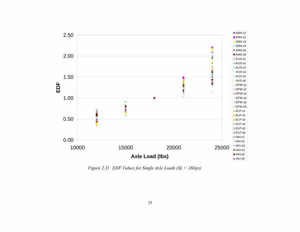
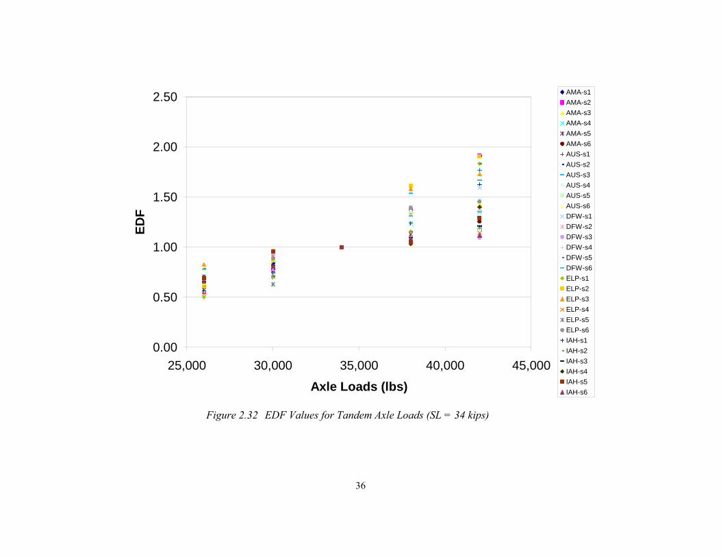
2.6.1 Rutting Using the results for rutting lives described in the previous sections, EDFs are obtained.
A plot showing all the EDF values for all the structures at all locations for single axle loads is shown in Figure 2.31 and those for the tandem axle loads are shown in Figure 2.32. It can be observed that as the axle loads increase, EDF values increase, indicating increased relative damage with the increase in axle loads. Furthermore, as the axle load increases, the EDF values increase at a higher rate, implying that the increase in axle loads causes a more than proportional increase in pavement deterioration.
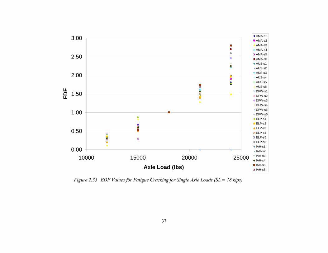
2.6.2 Fatigue Cracking EDF values were also calculated based on fatigue performance using 18 kips standard
axle load and 34 kips standard axle load. The plots of these EDF values are shown in figures 2.33 and 2.34 for single and tandem axles, respectively. It can be observed that as the axle load increases, EDF values increase at a higher rate, which implies that the increase in axle loads causes a more than proportional increase in pavement deterioration. While the results of fatigue are comparable to those of rutting, it is noticed that as the load increases, the EDF values increase more rapidly for fatigue than for rutting. Graphically, the EDF slope is higher for the case of fatigue compared to that of rutting.
Figure 2.34 EDF Values for Fatigue Cracking for Tandem Axle Loads (SL = 34 kips)
39
2.7 Regression Analysis and Applications
2.7.1 Regression Analysis Regression analyses were carried out to develop equations for estimating EDF. Linear
regression was carried out using various types of variable transformations such as linear, power, and exponential, in order to obtain the best model. These equations estimate EDFs as a function of relative axle load (L/18,000, where L is the load in lbs.), structural number (SN), locations, and axle type. Locations are used as categorical data, and Houston (IAH) was selected as the base location, with four dummy variables for locations: AMA, AUS, DFW and ELP. Axle Type (single axle and tandem axle) was also used as categorical data, with single axle being the base axle type and a dummy variable, Tandem, used for the axle type. The resulting models are discussed in the following sections.
2.7.1.1 Fatigue Cracking Upon analysis of various linear regression transformations, the logarithmic
transformation was selected to estimate fatigue based EDF. This model is represented by Equation 2.9.
It is observed from the final regression model for EDF in terms of fatigue that pavements
in AUS and AMA exhibit statistically significant different behavior in terms of EDF. On the other hand, the other three locations, IAH, DFW and ELP, are supposed to perform in similar fashion, while predicting fatigue-based EDF. Also, it can be seen from the slope parameters of the term representing the structural number that the fatigue based EDF increases as the structural number increases.
2.7.1.2 Rutting
EDF for rutting was also best represented using a logarithmic transformation. The final model is represented by Equation 2.10. It can be observed that the behavior of EDF for pavements in AMA is not significantly different from pavements in IAH. However, behavior of EDF of pavements in AUS, DFW, and ELP differ from pavements in IAH. The other variables, namely structural number, axle type, and relative load, were seen to have a statistically significant impact on the EDF model. The final model shows that for a given load and axle type, AUS and DFW have lower EDF values as compared to the other three locations.
40
{ }⎭⎬⎫
⎩⎨⎧
++−−−
=)(13.0)(09.0
)(15.0)(19.0)(38.003.3)*18000/ln()ln(
TandemELPDFWAUSSN
dLEDFrut
(2.10) Adjusted 91.02 =R
Another interesting observation in the case of rutting based EDF is that the axle type has
an additional impact on EDF after applying load corrections. The positive slope of the tandem axle term indicates that for tandem axles, the rutting based EDF value is more than that for single axles.
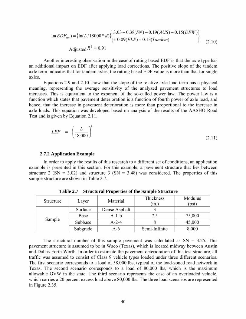
Equations 2.9 and 2.10 show that the slope of the relative axle load term has a physical meaning, representing the average sensitivity of the analyzed pavement structures to load increases. This is equivalent to the exponent of the so-called power law. The power law is a function which states that pavement deterioration is a function of fourth power of axle load, and hence, that the increase in pavement deterioration is more than proportional to the increase in axle loads. This equation was developed based on analysis of the results of the AASHO Road Test and is given by Equation 2.11.
4
000,18⎟⎠
⎞⎜⎝
⎛=
LLEF (2.11)
2.7.2 Application Example In order to apply the results of this research to a different set of conditions, an application
example is presented in this section. For this example, a pavement structure that lies between structure 2 (SN = 3.02) and structure 3 (SN = 3.48) was considered. The properties of this sample structure are shown in Table 2.7.
Table 2.7 Structural Properties of the Sample Structure
Structure Layer Material Thickness (in.)
Modulus (psi)
Surface Dense Asphalt 3 Base A-1-b 7.5 75,000
Subbase A-2-4 8 45,000 Sample
Subgrade A-6 Semi-Infinite 8,000
The structural number of this sample pavement was calculated as SN = 3.25. This pavement structure is assumed to be in Waco (Texas), which is located midway between Austin and Dallas-Forth Worth. In order to estimate the pavement deterioration of this test structure, all traffic was assumed to consist of Class 9 vehicle types loaded under three different scenarios. The first scenario corresponds to a load of 58,000 lbs, typical of the load-zoned road network in Texas. The second scenario corresponds to a load of 80,000 lbs, which is the maximum allowable GVW in the state. The third scenario represents the case of an overloaded vehicle, which carries a 20 percent excess load above 80,000 lbs. The three load scenarios are represented in Figure 2.35.
41
Scenario Single Tandem Tandem Total
1 10 24 24 58 2 12 34 34 80 3 16 40 40 96
Figure 2.35 Axle Loads (kips) for a Class 9 Vehicle Used in the Case Study
The fatigue- and rutting-based EDF values for single and tandem axles and the total EDF (EDF d 2.10 and are given in Table 2.8. Similarly, these values for DFW are shown in Table 2.9. The EDF values for AUS and DFW are linearly interpolated to get the estimated value of EDF for rutting and fatigue in Waco. The estimated EDF values for Waco are given in Table 2.10.
Table 2.8 Estimated EDF Values for AUS Fatigue- EDF Rutting- EDF
Scenario Single Tandem EDFfat Single Tandem EDFrut 1 0.20 0.38 0.96 0.39 0.55 1.49 2 0.33 1.00 2.33 0.52 1.00 2.52 3 0.54 1.66 3.86 0.83 1.33 3.49
Scenario Single Tandem EDFfat Single Tandem EDFrut 1 0.21 0.40 1.01 0.38 0.54 1.46 2 0.35 1.00 2.35 0.51 1.00 2.51 3 0.56 1.61 3.78 0.82 1.33 3.48
Table 2.10 Estimated EDF Values for Waco Scenario EDFfat EDFrut
1 0.99 1.48 2 2.34 2.52 3 3.82 3.49
Next, the fatigue life under single axle 18 kips load for Waco is estimated by linearly
interpolating the results of fatigue for AUS and DFW given in Section 2.5 and is found to be 18,885,808. Similarly, a rutting life of 2,862,648 is also estimated for Waco. These fatigue and rutting lives are then converted into number of trucks required for failure, using the EDF values given in Table 2.10.
The results of these estimated fatigue and rutting lives are then compared with those obtained by running the full simulation using the M-E Design Guide. The guide is simulated for
42
Waco, for the three load scenarios given in Figure 2.35. The failure criterion was based on 0.5” rutting and 10 percent fatigue cracking. The actual fatigue and rutting lives (in terms of number of trucks) obtained by running the full simulation are tabulated along with the estimated values in Table 2.11.
Table 2.11 Estimated vs. Actual Fatigue and Rutting Lives for Waco Fatigue Rutting
Comparing the results of the estimated lives with that obtained from the M-E Design
Guide, an error of 4 percent, 19 percent and 16 percent for the three scenarios, respectively, for fatigue is obtained. Similar comparison of rutting results gives an error of 6 percent, 20 percent and 20 percent for the three scenarios, respectively. Also, it is observed that as the load is increased from scenario 1 to scenario 2 (38 percent load increase), fatigue damage increases by 58 percent, while rutting damage increases by 41 percent. Also, if the load is increased from scenario 2 to 3 (20 percent load increase), the fatigue damage increases by 39 percent and the rutting damage increases by 28 percent. This indicates that the increase in pavement failure is more than proportional to the increase in axle loads.
43
3. Fatigue Testing
3.1 Introduction The objective of this part of the study was to model and evaluate the four point beam
bending fatigue tests carried out in accordance with the AASHTO TP-8 standard (AASHTO TP-8, 1996). The fatigue tests were conducted to acquire information about the fatigue performance of different mixes and evaluate the effect of modifiers on fatigue life. Recommendations have been made to outline a procedure for specimen fabrication as well as to investigate requirements by the TP-8 standard.
3.2 Literature Review
3.2.1 Modeling The following consists mostly of the excerpts from Report SHRP A-404 (Tayebali et al.,
1994) and Report SHRP A-003-A (Tangella et al., 1990), unless otherwise mentioned. These reports are an excellent compilation of literature on fatigue.
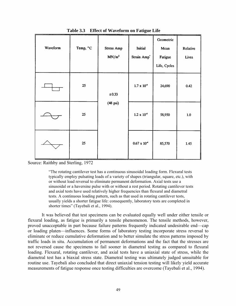
The fatigue resistance of an asphalt mix is its ability to withstand repeated bending without fracture. Fatigue fracture is the result of repeated tensile stresses and strains caused from traffic loading and thermal stresses in the pavement. For typical heavy duty pavements, fatigue cracking results from repeated tensile stresses or strains at the underside of the asphalt layers having a maximum value less than the tensile strength of the material. The maximum principal tensile strain is considered the primary determinant of fatigue cracking. Laboratory tests such as AASHTO provisional standard TP-8 (AASHTO TP-8, 1996) are available to subject an asphalt beam to repeated loading, while measuring the flexural stiffness of the beam to simulate the field loading conditions of an asphalt pavement. One application of loading and unloading is termed as a cycle.
“The fatigue characteristics of asphalt mixes are usually expressed as relationships between the initial tensile stress or strain and the number of load repetitions to failure—determined by using repeated flexure, direct tension, or diametral tests performed at several stress or strain levels” (Tayebali et al., 1994).
Monismith developed Equation 3.1 based on the same concept to predict the fatigue life of a specific mix based on the strain levels used for testing and initial mix stiffness (Monismith et al., 1985).
cb
f SaN ⎟⎟
⎠
⎞⎜⎜⎝
⎛⎟⎟⎠
⎞⎜⎜⎝
⎛=
00
11ε (3.1) Where, Nf : fatigue life (number of cycles to reach 50% of initial stiffness), εo : tensile strain, So : initial mix stiffness, and a,b,c : experimentally determined parameters.
44
Different models have been proposed based on the application of shift factors to Equation 3.1 to predict the service life of pavements with the failure criterion defined by the amount of cracking resulting from repeated loads. One model for fatigue cracking developed based on the AASHO Road test is illustrated by Equations 3.2 and 3.3, which are used for predicting fatigue cracking up to 10 percent of the wheel path area and more than 45 percent of the wheel path area, respectively (Finn et al., 1977).
( ) ⎟⎟⎠
⎞⎜⎜⎝
⎛−⎟
⎠⎞
⎜⎝⎛−=≤ − 3
*
6 10log854.0
10log291.3947.15%10log EN f
ε
(3.2)
( ) ⎟⎟⎠
⎞⎜⎜⎝
⎛−⎟
⎠⎞
⎜⎝⎛−=≥ − 3
*
6 10log854.0
10log291.3086.16%45log EN f
ε
(3.3) Where, N f : load applications to cause 10 or 45% fatigue cracking, ε : initial strain for applied stress, and E* : complex modulus.
Researchers have used the energy approach for predicting the fatigue behavior of the
asphalt mixes. It has been suggested that cumulative dissipated energy is related to the number of cycles to failure and, hence, can be used to describe results of different types of tests carried out under different test conditions with several types of asphalt mixes, to be described by a single mix-specific relationship (Van and Visser, 1977). Dissipated energy also has greater conceptual appeal than a simple strain indicator because it captures both elastic and viscous effects. The dissipated energy per cycle per unit volume can be expressed by Equation 3.4:
φεσπ sin...=W (3.4) Where, W : dissipated energy in the loading cycle, σ : stress amplitude, ε : strain amplitude, and Φ : phase angle between the stress and strain wave signals.
During a controlled strain test, the stress amplitude and the phase angle change. The total
dissipated energy is calculated integrating the functions of the stress and phase angle over the number of loading cycles concerned. This integration is approximated by a summation of energy into fixed intervals of constant cycles, i.e., cycles in which the stress and phase angle in that interval are assumed to be nearly constant (Van and Visser, 1977).
The cumulative dissipated energy as calculated above is related to the number of cycles to failure as illustrated by Equation 3.5.
( )zfN NAW = (3.5)
Where, N f : fatigue life (number of cycles to 50% of initial stiffness), WN : cumulative dissipated energy at failure, and A, z : experimentally determined coefficients.
45
Therefore, such an approach would make it possible to predict the fatigue behavior of mixes in the laboratory over a wide range of conditions from the results of a few simple fatigue tests, such as four point beam bending fatigue tests (Tayebali et al., 1994).
The theory of linear elasticity can be used to estimate critical stress and strain in the pavement for the fatigue analysis. Linear elastic theory characterizes the behavior of the asphalt mix by its modulus of elasticity and Poisson’s ratio. Although asphalt is viscoelastic in nature, fatigue distress accumulates most rapidly under moderate to cool temperatures and rapid traffic loading. This justifies the use of the linear elastic theory to provide reasonable estimates. The use of linear viscoelastic modeling can increase the accuracy of the estimates and is particularly useful for estimating the energy dissipated during each loading cycle for structural analysis (Tayebali et al., 1994).
“Under compound or mixed loading; due, for example, to multiple temperatures or stress or strain levels; cracking in a given mix is initiated when the linear summation of cycle ratios equals 1” (Tayebali et al., 1994).
This concept is captured by Equation 3.6:
∑ =i i
i
Nn
1 (3.6)
Where, ni : number of applications at strain εi, and Ni : number of applications to failure at strain εi.
3.2.2 Tests Available for Fatigue There are various methodologies for measuring the fatigue behavior and response of
asphalt concrete. The general categories include (Tayebali et al., 1994): 1) “Simple flexure with a direct relationship between fatigue life and stress/strain
developed by subjecting beams to pulsating or sinusoidal loads in either a third or center-point configuration; rotating cantilever beams; and trapezoidal cantilever beams subjected to sinusoidal loading.
2) Supported flexure with a direct relationship between fatigue life and stress/strain developed by loading beams or slabs that are supported in various ways to directly simulate in situ modes of loading and sometimes to simulate a more representative stress state.
3) Direct axial with a direct relationship between fatigue life and stress/strain developed by applying pulsating or sinusoidal loads, uniaxially, with or without stress reversal.
4) Diametral with a direct relationship between fatigue life and stress/strain developed by applying pulsating loads to cylindrical specimens in the diametral direction.
5) Triaxial with a direct relationship between fatigue life and stress/strain developed by testing similar to direct axial testing but with confinement.
6) Fracture tests and the use of fracture mechanics principles to predict fatigue life.
7) Wheel-tracking tests, including both laboratory and full-scale arrangements, with a direct relationship between the amount of cracking, the number of load
46
applications, and the measured and/or computed stress/strain. For full-scale tests, both linear and circular track configurations have been used.”
Proper specimen fabrication is important, as specimens should be able to reasonably duplicate the asphalt composition, density, and engineering properties. The compaction temperature is typically selected such that the asphalt viscosity is 500 ± 50 cSt (ASTM, 2004). Compaction methods presently being utilized to fabricate test specimens include the following: (1) static compaction, (2) impact compaction, (3) kneading compaction, (4) gyratory compaction, and (5) rolling-wheel compaction.
Different methods are adopted in laboratory tests by which stress and strain are permitted to vary during repetitive loading. These methods range from the controlled stress mode, where the load or stress amplitude remains constant during testing, to controlled-strain mode, where the deformation or strain amplitude is constantly maintained. The testing temperature affects the mixture stiffness, and hence affects the test results. Attempts have been made to determine the mode of loading that best simulates actual pavement conditions (Monismith et al., 1985). Researchers have evaluated several characteristics of the two modes of loading and a brief summary is presented in Table 3.1. The mode-of-loading effect is more likely a result of differences in the rates of crack propagation than to differences in the times to crack initiation. The mixes are subjected to lower strain levels in situ as compared to the strain levels used for fatigue tests. However, testing at two or more higher strain levels is sufficient to indicate the behavior at the lower levels (Tayebali et al., 1994).
A summary of the influence of selected mixture variables on fatigue response is contained in Table 3.2. Air void content has been identified as an important factor affecting fatigue life of an asphalt mixture. Lower air voids lead to higher fatigue lives, but the air voids are limited to a minimum of 3 percent (Tangella et al., 1990), as sufficient voids should be provided to allow for a slight amount of additional compaction under traffic and a slight amount of asphalt expansion due to temperature increases, without flushing, bleeding, or loss of stability.
47
Table 3.1 Comparison Controlled-Stress and Strain Loading
VARIABLES CONTROLLED-STRESS (LOAD)
CONTROLLED-STRAIN (DEFLECTIONS)
Thickness of asphalt concrete layer
Comparatively thick asphalt bound layers
Thin asphalt-bound layer, < 3 inches
Definition of failure; number of cycles
Well-defined since specimen fractures
Test is discontinued when the load level has been reduced to a
proportion of its initial value
Scatter in fatigue test data Less scatter More scatter
Required number of specimens Smaller Larger
Simulation of long-term influences
Long-term influences such as aging lead to increased
stiffness and increased fatigue life
Long-term influences leading to stiffness increase will lead to
reduced fatigue life
Fatigue life (N) Generally shorter life Generally longer life
Effect of mixture variables More sensitive Less sensitive
Rate of energy dissipation Faster Slower
Rate of crack propagation Faster than occurs in situ More representative of in situ
conditions Beneficial effects of rest
periods Greater beneficial effect Lesser beneficial effect
Source: Tangella et al., 1990
Higher temperature lowers fatigue life in the case of thick asphalt pavements but increases fatigue life for thin pavements (Monismith et al., 1985). The optimum asphalt content is usually determined by balancing the fatigue and rutting considerations for a mix. The optimum asphalt content to obtain a maximum fatigue life is generally higher than that required based on rutting considerations. Therefore, the asphalt content should be as high as possible with due consideration to stability. Thin pavements require flexible asphalts and open-graded aggregates as compared to thick pavements, which require stiff asphalts and dense-graded aggregates (Tangella et al., 1990).
Testing to failure of the sample under cyclic loading is necessary in order to accurately measure the fatigue response of asphalt-aggregate mixes. The most popular forms of loading used for fatigue tests are pulse and sinusoidal loading. Pulsed loading has the advantage of introducing rest periods, which permits stress relaxation similar to that permitted under in-service traffic loading. Rest periods were introduced into fatigue testing as storage periods (for conventional continuous loading tests) and intermittent loading. Several authors found that rest periods lead to longer fatigue lives in laboratory testing. Bonnaure (1982) carried out a systematic investigation to better understand the effect of rest periods on the fatigue life of
48
mixes. He identified various parameters that influence fatigue life in his experiment including: rest period, test temperature, bitumen and mix type, and test mode. The equipment used in this experiment was the dynamic four point bending apparatus for rectangular beams. By incorporating rest periods to the testing procedure and introducing longer rest periods, Bonnaure noticed “a shift of the fatigue line to higher levels, showing the beneficial effect of rest periods on fatigue life.” The benefit seemed to reach a limit or maximum around a rest period equal to 25 times the loading time. The disadvantage of pulsed loading is the characteristic 1 to 2 Hz testing frequency, which is not rapid enough for accelerated performance testing in fatigue.
Table 3.2 Stiffness and Fatigue Response of Asphalt Mixtures
Effect of Change in Factor
Factor Change in Factor On
Stiffness
On Fatigue Life in Controlled-Stress Mode of Testing
On Fatigue Life in Controlled-Strain Mode of Testing
Air Void Content Decrease Increase Increase Increase
Temperature Decrease Increase Increase Decrease Source: Tangella et al., 1990
It has been concluded in SHRP Project A003A that a loading time in the range of 0.04 to 0.1 second is appropriate for fatigue testing. Test results confirmed that mix effects on fatigue performance were similar in either pulsed or sinusoidal loading (Tayebali et al., 1994). Table 3.3 demonstrates the effect of shape of waveform on fatigue life.
For heavy duty pavements, an increase in mixture stiffness increases the fatigue life, provided other variables remain constant. Epps (1969) compared the fatigue performance of specimens (four point beam bending tests) obtained from pavements subjected to actual traffic loading to that of laboratory specimens of similar composition. It was found that the increased stiffness of the field mix induced due to aging compensates for the effect of higher in situ air voids and damage caused by traffic loading. On the contrary, in cold weather conditions, aging induced stiffness reduces the asphalt’s cracking resistance (because of increased brittleness). The field projects of Epps’ study (Gonzales By-pass and Morro Bay) were not located in cold environments; hence the effect of cold environments was not captured by his experiments.
Densification of a paving mixture by traffic in service is also likely to affect its fatigue response. Raithby and Sterling (1972) found, for example, that traffic compaction in a large test slab increased fatigue life for a given stress level by a factor of three and increased the dynamic stiffness by 60 percent. The effect on fatigue life is due both to the increase in stiffness and the decrease in air voids.
49
Table 3.3 Effect of Waveform on Fatigue Life
Source: Raithby and Sterling, 1972
“The rotating cantilever test has a continuous sinusoidal loading form. Flexural tests typically employ pulsating loads of a variety of shapes (triangular, square, etc.), with or without load reversal to eliminate permanent deformation. Axial tests use a sinusoidal or a haversine pulse with or without a rest period. Rotating cantilever tests and axial tests have used relatively higher frequencies than flexural and diametral tests. A continuous loading pattern, such as that used in rotating cantilever tests, usually yields a shorter fatigue life: consequently, laboratory tests are completed in shorter times” (Tayebali et al., 1994).
It was believed that test specimens can be evaluated equally well under either tensile or flexural loading, as fatigue is primarily a tensile phenomenon. The tensile methods, however, proved unacceptable in part because failure patterns frequently indicated undesirable end—cap or loading platen—influences. Some forms of laboratory testing incorporate stress reversal to eliminate or reduce cumulative deformation and to better simulate the stress patterns imposed by traffic loads in situ. Accumulation of permanent deformations and the fact that the stresses are not reversed cause the specimens to fail sooner in diametral testing as compared to flexural loading. Flexural, rotating cantilever, and axial tests have a uniaxial state of stress, while the diametral test has a biaxial stress state. Diametral testing was ultimately judged unsuitable for routine use. Tayebali also concluded that direct uniaxial tension testing will likely yield accurate measurements of fatigue response once testing difficulties are overcome (Tayebali et al., 1994).
50
3.2.3 Polymer Modified Binders
Polymer modified binders (PMBs) are commonly used today in an effort to reduce early pavement distress and to extend service life by enhancing the binder’s adhesion, cohesion, and elasticity (King et al., 1986). A polymer is a very large molecule made by the chemical reaction of many (poly) smaller molecules (monomers) with each other. The addition of polymers alters the rheological properties of asphalt cement so that it can retain sufficient flexibility at low temperatures while attaining a marked resistance to plastic-viscous deformation at high temperatures. It makes the binder more resistant to temperature variations, extreme weather, and high traffic loads. The polymer is dispersed in the binder by adding it to the fluid binder at a temperature of 160-175 ºC (320-347 °F) and stirring with a high shear mechanical stirrer. They can be of the plastomeric (elastic structure derived from crystallinity and entanglements) or elastomeric (elastic structure derived from temporary and permanent cross links) type. Elastomers resist deformation from applied stress by stretching and recovering their shape quickly when stress is removed. Some examples of elastomeric polymers are styrene-butadiene-styrene copolymer (SBS), styrene-butadiene rubber (SBR), Tire Rubber (TR), and ethylene ter polymer (ETP). Plastomers, on the other hand, have a tough, rigid, three-dimensional network that is resistant to deformation. Some popular plastomers are polyethylene (PE), ethyl vinyl acetate (EVA), and ethyl butyl acrylate (EBA).
Lewandowaski (1994) and Jones (2000) have identified the major reasons for the addition of polymers in separate studies. Some polymers help in reducing viscosity at laying temperatures and in increasing the stability of the mixes. Others improve the fatigue and abrasion resistance of the mixes. It was found (Maccarrone et al., 1995) that elastomeric binders (e.g., SBS) improve both rut resistance and fatigue life through increased ability to recover. Plastomeric binders (such as EVA) improve rut resistance without compromising fatigue properties. Maccarrone also concluded that temperature susceptibility of SBS- and EVA-modified binders are similar to each other but are substantially lower than for the unmodified bitumen. SHRP specification parameters of G* (complex modulus)/sinδ (phase angle) for rutting and G*.sinδ for fatigue cracking appear to be relevant for PMBs, as they broadly indicate relative performance of the PMBs compared to unmodified binders. G* can be considered as the total resistance of the binder to deformation when repeatedly sheared (Roberts et al., 1996).
Terrel and Walter (1986) have illustrated the use of polymer modified asphalts in chip seals, slurry seals, dense and open hot mix overlays, and special mastic and patching systems. The properties of the modified binder permit applications of mixtures to maintenance or repair situations that are much more versatile than with the conventional asphalts. Smaller quantities are usually required, which offsets the costs of asphalt. They also concluded that longer service lives are achieved by associating modified asphalt with high quality aggregates and construction methods. Polymers provide considerable improvement in the physical properties of the binder as well as binder aggregate combinations. These include improved adhesion and cohesion, improved temperature susceptibility, improved modulus or stiffness, increased resistance to fatigue and rutting, and increased durability.
King et al. (1986) concluded that the selection of the appropriate type and amount of polymer modifier offers a valuable tool in the improvement of binders in problematic situations such as heavy traffic, high stress, poor aggregates, and variable climates. The elasticity, tensile strength, adhesivity, and resistance to temperature susceptibility of the binder impart improved stiffness moduli, rutting resistance, fatigue life, adhesion, and stripping resistance to the polymer
51
modified bituminous mix. Test results have been consistent with numerous field trials in demonstrating the effectiveness of the polymer modification.
3.3 Fatigue Testing
3.3.1 Introduction The main purpose of carrying out the four point beam bending fatigue tests was to
analyze the fatigue response of the Type D asphalt mixture used for the construction of the HB2060 pads at UT Austin’s J.J. Pickle Research Center. In addition, this mix was compared to other selected mixes typically used by TxDOT. The data collected was compiled into a database with all relevant information stored and accessible in a user-friendly format.
The tests were also carried out to evaluate AASHTO provisional standard TP-8 (AASHTO, 1996) and to identify the advantages of using modified binders with respect to the fatigue life of the various mixes. The purpose of the tests also included quantification of the variability associated with the results and identification of the sources of variability of the results.
3.3.2 Materials Used The first ten tests consisted of premanufactured mixes, designated as APT mixes,
obtained from the pavement constructed at UT Austin’s J.J. Pickle Research Center for APT with the TxMLS. In addition, twenty-seven fatigue tests were carried out on the “Type D” mix with three different binders, namely, 76-22 SBS, 76-22 TR and PG 64-22 (base binder for the first two binders). As mentioned in the literature review, SBS and TR are modifiers added to the base binder PG 64-22 to enhance the fatigue life of the mix. Six fatigue tests were also carried out on “Superpave Type D” mix with PG 64-22 binder at two different binder contents. “Superpave Type D” and “Type D” are mix designations provided by TxDOT with gradations shown in Tables 3.4 and 3.5 (TxDOT, 2004a). The blend column corresponds to the gradation of the mix used for testing, and the target column corresponds to the TxDOT specifications. Both Type D mix and Superpave Type D mix used for testing satisfy the target gradation.
52
Figure 3.1 Fatigue beam testing apparatus
3.3.3 AASHTO TP-8 The testing procedure consists of manufacturing the beams and then testing them by the
fatigue testing apparatus, as shown in Figure 3.1. The AASHTO TP-8 standard provides procedures for determining the fatigue life and fatigue energy of 380 mm (15 in.) long by 50 mm (2.0 in.) thick by 63 mm (2.5 in.) wide hot mix asphalt (HMA) beam specimens sawed from laboratory or field compacted HMA and subjected to repeated flexural bending until failure. The fatigue life and failure energy determined by this standard can be used to estimate the fatigue life of HMA pavement layers under repeated traffic loading.
The four point beam bending test procedure (at constant strain) entails applying repeated loading and unloading to a beam specimen until the flexural stiffness of the specimen reduces to a predetermined value (usually 50 percent of original stiffness). One such application of loading and unloading is termed as a load cycle. The load is so applied that the specimen experiences constant strain amplitude during each loading cycle. Repeated sinusoidal loading at a frequency range of 5 to 10 Hz is usually applied, subjecting specimens to four point bending with free rotation and horizontal translation at all load and reaction points, with the flexural stiffness estimated after every ten cycles.
The constant strain level can be fixed from 250-750 micro strains as specified by AASHTO TP-8 with specimens tested in an environmental chamber at 20 ± 0.5 ºC (68 ± 1 °F). The flexural stiffness measured after the first fifty conditioning cycles is termed as initial stiffness, and 50 percent of the initial stiffness is termed as termination stiffness or point of failure. The test is stopped after the termination stiffness has been achieved.
AASHTO TP-8 specifies the desired void content of 7 ± 0.5 percent in the beam, which is representative of the void content of a new pavement after construction. Based on the void content, the amount of mix to be compacted to a specified volume can be computed by volumetric calculations. The volume is determined based on the volume of the mold used for compaction. The various volumetric equations involved are the following:
54
b
sbb P
MPM
−=
1*
(3.7) bst MMM += (3.8)
V = l * b * h (3.9)
mm
mb
GG
VIM −= 1 (3.10)
Where : Mb : mass of binder, Mt : total mass of mix, Pb : percentage of binder by weight of the mix, Ms : mass of aggregate, l,b,h : dimensions of the mold, V : volume of the mold, Gmb : bulk specific gravity of compacted mix, Gmm : maximum theoretical specific gravity, and VIM : voids in mix.
The mixing process is comprised of mixing the desired proportions of the aggregates
(according to the required gradation) together to form a blend and heating the blend up to the mixing temperature provided in Table 3.6. The mixing temperatures are determined from the temperature-viscosity curve obtained by measuring the rotational or Brookfield viscosity at two or more temperatures. The Brookfield viscosity is determined by measuring the torque required to maintain a constant rotational speed (20 rpm) of a cylindrical spindle while submerged in an asphalt binder at constant temperature. The measured torque is directly related to the viscosity of the binder sample, which is automatically displayed by the viscometer (Roberts et al., 1996).
Table 3.6 Binder mixing and compaction temperatures PG76-22S PG76-22TR PG64-22
The mix is then aged in the oven for 4 hours at 135 ºC (275 °F) to simulate the aging in
the field in the time taken to transport the mix from the plant to the pavement. Two thousand grams of the mix is taken out (in total) from the pans after 4 hours for tests to determine theoretical maximum density in accordance with AASHTO T 209 (AASHTO, 1999). The AASHTO T 209 test method covers the determination of the theoretical maximum specific gravity (Gmm) and density of uncompacted bituminous paving mixtures at 25 °C (77 °F). The required amount of mix is then heated up to the compaction temperature, provided in Table 3.6, along with the mold. The heated mix is poured into the mold, and then the mold is placed in the Asphalt Vibratory Compactor (AVC) and compacted, as shown in Figure 3.2.
The AVC was designed to compact rectangular and cylindrical specimens of asphalt mixes to be used in conjunction with the Asphalt Pavement Analyzer (APA). The AVC compacts samples at the same amplitude, frequency and relative weight that a contractor applies with a vibratory compactor on the roadway (AVC Manual, 2003). After the samples are
55
compacted, they are extracted with the help of an air cylinder. After compaction, the slabs are left overnight and then tested for their bulk density.
Figure 3.2 Automatic Vibratory Compactor
The slabs are then sawed to derive two beams 15 in. long by 2 in. high by 2.5 in. wide. The slabs are cut such that each beam side is sawed. The beams are then conditioned for 7 days in a temperature control chamber at 68 ºF. They are then tested in accordance with AASHTO TP-8. Based on experimentation, strain levels of 250 and 500 microstrains were considered appropriate for mixes with unmodified binders, and 500 and 750 microstrains were considered appropriate for modified binders. These strain levels were selected so that the duration of the test is appropriate (it neither fails in less than 100,000 cycles as specified by AASHTO and does not continue on for more than one week). The loading frequency was fixed at 10 Hz and the temperature chamber maintained at 68 ± 1 °F. The loading waveform was selected as sinusoidal as shown in Figure 3.3 based on AASHTO recommendations and the test was terminated at a stiffness level of 15 percent instead of the traditional 50 percent.
The beam is subjected to bending in a constant strain test. It can be observed in Figure 3.3 that the strain is not in phase with the load, indicating the viscoelastic nature of asphalt mix, and the lag represents the phase angle of asphalt mix. The phase angle provides a relative indication of the viscous and elastic behavior of the asphalt mix. Materials with a phase angle of 90 degrees are completely viscous; while materials with a phase angle of 0 degrees are completely elastic.
56
Waveforms
-200
-150
-100
-50
0
50
100
150
200
250
0 20 40 60 80 100 120
Time (msec)
stress (KPa)Microstrain
Figure 3.3 Sinusoidal loading waveform
3.3.5 Observations Figure 3.4 depicts a typical change in the flexural stiffness with load during one of the
experiments. It can be observed that there is a dip in the curve which, in this case, is located after the 50 percent stiffness point. This dip is important to capture as it leads to a significant loss of strength with only a few repetitions. Hence, it is recommended that the duration of the fatigue tests be extended until 15 percent to 20 percent of initial stiffness is reached, thus capturing this dip.
Figure 3.4 A typical flexural stiffness – cycles curve obtained from a fatigue test.
57
A typical fatigue curve (obtained for the APT mix) is illustrated in Figure 3.5. The test results can be used to verify the traditional fatigue model given by Equation 3.1. Table 3.7 depicts all the beams tested. The last ten rows of Table 3.7 have been used to develop the fatigue curve shown in Figure 3.5.
Figure 3.5 A typical fatigue curve for the selected APT mix.
0
1
2
3
4
5
6
7
2.45 2.5 2.55 2.6 2.65 2.7 2.75 2.8 2.85 2.9
log (microstrains)
log
(Num
ber o
f cyc
les)
76-22 SBS64-2276-22 TR
300 microstrains
500 microstrains
750 microstrains
Figure 3.6 Fatigue curves for Type D mix (50% stiffness)
58
Table 3.7 Experimental Results
Mix Type Void
content (%)
Initial stiffness
Number of load cycles to failure (50% stiffness)
Number of load cycles to failure (20% stiffness)
strain level
Type D 76-22 S 8.3 4013 1,668,100 2,657,320 500 Type D 76-22 S 8.4 6885 441,570 922,570 500 Type D 76-22 S 8.5 5585 2,486,310 Did not reach 500 Type D 76-22 S 10.0 4510 50,370 353,450 500 Type D 76-22 S 8.3 4850 156,670 448,400 750 Type D 76-22 S 8.5 6429 42,870 261,240 750 Type D 76-22 S 10.2 4240 73,940 597,000 750 Type D 76-22 S 10.3 3903 39,600 144,950 750 Type D 64-22 10.5 5008 256,050 364,470 500 Type D 64-22 12.6 4390 Did not reach Did not reach 300 Type D 64-22 12.8 3800 1,011,790 2,220,250 500 Type D 64-22 11.6 5781 2,781,050 3,111,540 300 Type D 64-22 5.0 7016 2,840,090 Did not reach 300 Type D 64-22 5.0 6210 129,320 180,000 500 Type D 64-22 2.5 6208 2,435,940 2,690,000 300 Type D 64-22 2.0 8551 72,730 451,970 500 Type D 64-22 4.9 8760 Did not reach Did not reach 300 Type D 64-22 5.1 8254 68,830 290,620 500 Type D 64-22 4.4 8254 Did not reach Did not reach 300 Type D 64-22 3.8 9482 77,820 242,660 500 Type D 64-22 11.6 3898 Did not reach Did not reach 300
Type D 76-22 TR 13.1 7526 Did not reach Did not reach 500 Type D 76-22 TR 13.1 7544 19,690 118,850 750 Type D 76-22 TR 12.5 7455 11,330 52,740 750 Type D 76-22 TR 12.5 8491 337,540 1,617,660 500 Type D 76-22 TR 8.9 10606 361,680 1,196,120 500 Type D 76-22 TR 8.9 11153 15,800 139,100 750
Superpave 6.3 7833 128,330 N/A 500 Superpave 6.3 7408 137,500 N/A 500 Superpave 6.8 7745 Did not reach N/A 250 Superpave 6.8 8222 Did not reach N/A 250 Superpave 8.1 6375 121,610 N/A 500 Superpave 8.1 7206 56,370 N/A 500
The termination stiffness in accordance with AASHTO TP-8 is considered to be 50 percent of initial stiffness for the data presented in Figure 3.6. It can be observed from the curves that the curves corresponding to 76-22 SBS and 64-22 have similar slopes. However, 76-22 SBS has a higher intercept than 64-22. Hence, the curves indicate that the 76-22 SBS binder performs better than the base binder 64-22. It seems, however, that the TR binder outperforms both the other binders at lower strain levels and underperforms at higher strain levels. These predictions involve extrapolation of data, and hence, are premature. It should be noted that these curves are constructed based on only two strain levels and a high associated variability. Moreover, the void contents of the different beams varied by up to 4 percent, and there are only a few data points for each strain level. The fatigue curves for a termination stiffness of 20 percent of initial stiffness are plotted in Figure 3.7.
0
1
2
3
4
5
6
7
2.45 2.5 2.55 2.6 2.65 2.7 2.75 2.8 2.85 2.9
log (microstrains)
log
(num
ber o
f cyc
les)
76-22 SBS64-2276-22 TR
300microstrains
500microstrains
750microstrains
Figure 3.7 Fatigue curve for Type D mix (based on 20% stiffness)
Figures 3.6 and 3.7 show that changing the termination criteria changes the nature of the fatigue curves. The curves for 76-22 TR and 76-22 SBS are intersecting in Figure 3.7, which is not the case in Figure 3.6. The termination criterion is a very important characteristic of the test and further research is warranted to determine a rigorous termination criterion.
It can be observed from the Superpave Type D results that increasing the binder content (for binder contents greater than the optimum binder content) seems to increase the fatigue life as anticipated. The optimum binder content has been defined as the asphalt content that produces 4 percent air voids at the design number of gyrations (Roberts et al., 1996). This is the number of gyrations expected to produce a density in the mix that is equivalent to the expected density in the field after the indicated amount of traffic. The design number of gyrations for the current experiment was 100 gyrations with an optimum binder content of 5.1 percent. Figure 3.8 shows the plot of the binder content versus the number of cycles to failure for the Superpave Type D mix for two different binder contents. The mixes at the other two binder contents are yet to be tested. As expected, the binder content of 5.5 percent seems to lead to a lower fatigue life compared to 6 percent. It is, however, also observed that the variability at 5.5 percent is also very high compared to 6 percent. Hence, the curve does not lead to a concrete conclusion.
60
0
20,000
40,000
60,000
80,000
100,000
120,000
140,000
160,000
5.4% 5.5% 5.6% 5.7% 5.8% 5.9% 6.0% 6.1%
binder content
num
ber o
f cyc
les
Figure 3.8 Superpave Type D fatigue results.
As mentioned earlier, it has been suggested that, for a given failure criterion, the cumulative dissipated energy is related to the number of cycles to failure and can be used to compare results of different types of tests carried out under different test conditions by a single mix-specific relationship. If this hypothesis is true, the cumulative dissipated energy should not depend on the strain levels of the fatigue tests carried out on a specific mix: the dissipated energy at failure should be a characteristic of the mix. To test this hypothesis, a regression analysis was carried out with the cumulative dissipated energy at failure (cycles to reach 50 percent of initial stiffness) as the dependent variable, with the strain as the independent variable. The regression equation developed is depicted by Equation 3.11. The data are shown in Table 3.8.
)2276(*40.2)2276(*87.58*44.094.33150 TRSstrainW −−−+−= (3.11) Where, W50 : cumulative energy dissipated at 50% of initial stiffness, Strain : strain level of the test, and 76-22S, 76-22TR : dummy variables (64-22 is kept as the base)
Table 3.9 depicts the regression statistics. The relatively low t-statistics of the parameters
associated with the dummy variables seem to indicate that the dissipated energy at failure for the modified (76-22S and 76-22TR) and unmodified mixtures are not significantly different. Even more interesting is the fact that the sign of 76-22TR is negative, indicating that less energy is dissipated in this case as compared with the unmodified mixture. It should be noted, however, that this analysis is based on a limited number of tests. The few data points and high associated variability can be the causes of these unexpected results.
61
Table 3.8 Data used for cumulative dissipated energy analysis Cumulative
Dissipated Energy at 50% of initial stiffness (MPa)
Cumulative Dissipated Energy at 20% of initial stiffness (MPa)
Strain level used for the test
(microstrains) Mix Type
383 567 500 Type D 76-22 S 40.6 243 750 Type D 76-22 S 108 257 750 Type D 76-22 S 19.5 55 750 Type D 76-22 S 6.79 55.6 500 Type D 76-22 S 169 291 500 Type D 76-22 S 27 55.6 750 Type D 76-22 S 159 278 500 Type D 64-22 130 210 300 Type D 64-22 82.5 109 500 Type D 64-22 403 424 300 Type D 64-22 31.8 99.6 500 Type D 64-22 40.3 103 500 Type D 64-22 10.3 23.6 750 Type D 76-22 TR 141 562 500 Type D 76-22 TR 193 557 500 Type D 76-22 TR 22.3 129 750 Type D 76-22 TR 48 54 300 Type D 76-22 TR
Table 3.9 Regression Statistics
R Square 0.290 Standard Error 109.911 Observations 18
Df SS MS F Significance FRegression 3 69071.64 23023.8 1.906 0.175 Residual 14 169126.82 12080.4
The effect of the test strain level can also be analyzed based on the results in Table 3.9. At a 5 percent level, the strain level has a significant effect on the cumulative energy dissipated at failure and, hence, the cumulative energy is not independent of the test characteristics as
62
originally hypothesized. However, the associated p-value indicates that for any level lower than 4.3 percent, the effect of the strain level will not show as significant.
Finally, to investigate the effect of the failure criterion on the cumulative energy at failure, another regression analysis was carried out using as the failure criterion the number of cycles to reach 20 percent of the initial stiffness. A similar analysis to the one before was carried out. The data for the regression is illustrated in Table 3.8, and the regression equation is depicted by Equation 3.12.
Table 3.10 illustrates the regression statistics for this equation. It can be observed now that the strain does not have a statistically significant effect on the cumulative dissipated energy at failure (low associated t-statistics). Hence, extending the test termination criterion to 20 percent of initial stiffness can lead to the use of the cumulative energy as a criterion independent of the test characteristics for a specific mix.
The parameters associated with the dummy variables, however, have low associated t-statistics. This would indicate that the use of modifiers in the mixtures does not have a statistically significant effect on improving the performance of the mixtures subjected to repeated bending. Since these conclusions are based on a few tests with high associated variability, further testing needs to be carried out to investigate the use of the cumulative energy.
Table 3.10 Regression Statistics
R Square 0.172 Standard Error 189.267 Observations 18
Df SS MS F Significance FRegression 3 96935.614 32311.8 0.902 0.465 Residual 14 501506.806 35821.9
Total 17 598442.420
Coeff Standard
Error t Stat P-value Intercept 432.956 166.874 2.595 0.021
Another potential method for determining failure involves the quantification of the variation of the phase angle (Figure 3.9). It is apparent that the variation increases with the number of loading cycles, hence, the variance of the data could be used as a measure of damage. The phase angles were plotted for all tests, and they all show an increase in variance. The reason for such phenomenon is unknown at this time and could be related to the test set up, however, it is the authors’ opinion that this increased variability is related to damage in the specimen.
Figure 3.9 Phase angle variation during a given test
3.3.6 Model Developed In this section, and based on the entire data set presented in Table 3.7, a model was
developed as given by Equation 3.13 as follows:
SUPERTR
SstiffnessstrainN f
*42.1)2264(*57.1)2276(*58.2
)2276(*40.2)ln(*08.2)ln(*68.595.63)ln(
+−+−
+−+−−=
(3.13)
Where, N f : number of cycles to 50% stiffness, strain : strain value at the test, and stiffness : initial stiffness at the starting of the test. 76-22S, 76-22TR, 64-22, SUPER : dummy variables.
The summary statistics are provided in Table 3.11. The regression equation shows that an
increase in strain leads to a decrease in fatigue life. Interestingly, an increase in initial stiffness also leads to a decrease in fatigue life. The use of dummy variables to represent the various mixes tested in this study is useful in revealing the significant difference in performance that is expected for each mixture.
Some unexpected results were found during this exercise, mainly due to the lack of experience in producing beams at the desired density. Most of the beams are usually prepared by trial and error procedure, i.e., different amounts of mix are poured into the mold and compacted and then the densities are measured, and thus the correct amount of mix is determined to obtain the target air void content. It is not possible to obtain exactly the same void content in the slab as predicted by the theoretical calculations. However, it is possible to achieve a target range of ±1.5 percent with respect to the desired void content. Since the air void content is of paramount importance for fatigue performance, it is believed that this variability is not acceptable. As the
64
researcher becomes more familiar with the compaction equipment, it is anticipated that air void variability could be kept below ± 0.5 percent.
3.3.7 Database development For further research, a database was developed using Excel Macros (Visual Basic), which
consists of all the measured data stored in a prescribed format. The database has a user-friendly interface and is capable of producing results of queries regarding all the possible values of the experimental variables. Table 3.11 provides all the variables stored in the database. The database can also link to the individual fatigue test files, thus enabling the user to view the test results in detail.
65
Table 3.11 Variables stored in the database Variables Explanation
Date of compaction Slab Sample ID The ID assigned to slab (numeric)
Mix Type The type of mix compacted (APT, Type D etc) Mt The total mass of the mix used for compaction
Binder type The PG binder specification Binder content (target) The calculated binder content to be added
Binder content (achieved) The actual binder content poured into the mix Aging time The aging time and temperature Target voids The voids desired in the slab
Rice The maximum theoretical gravity of the mix Voids in slab The achieved voids in slab
Beam ID The ID assigned to beam (alpha numeric) Voids in beam The voids achieved in the beam
Fatigue Test Status Y if the fatigue test has been carried out in the beam, N for
vice versa Fatigue test no Associated fatigue test number of the test
Comments Any additional info about the test Sample and Cyclometer
mass in air Rice measurements Pycnometer mass in air Rice measurements
Sample mass in air Rice measurements Sample and Pycnometer
filled with water Rice measurements Pycnometer filled with water Rice measurements
Sample in water Rice measurements Sample volume Rice measurements
Dry The dry weight of the slab (Bulk density calculation) Submerged The submerged weight of the slab (Bulk density calculation)
SSD The SSD weight of the slab (Bulk density calculation) Density The bulk density of the slab
Bdry The dry weight of the beam (Bulk density calculation) Bsumberged The submerged weight of the beam (Bulk density calculation)
BSSD The SSD weight of the beam (Bulk density calculation) Bdensity The density of the beam (Bulk density calculation)
66
67
4. Conclusions and Recommendations
4.1 Conclusions This research study was initiated with the objective of testing the HB2060 pads
constructed at UT Austin’s J.J. Pickle Research Center. Four pads were selected for testing under the TxMLS. By the time the research project started, the TxMLS was undergoing evaluation and renovation. Unfortunately, the equipment was not ready for testing within the timeframe of the project. For this reason, this report only covers two research related aspects: 1) the development of a methodology for determining equivalent damage by using the recently developed M-E Design Guide, and 2) evaluation of the laboratory fatigue performance of the asphalt mixture used for the construction of the HB2060 test pads and its comparison with other typical TxDOT mixes.
4.2 Equivalent Damage The M-E Design Guide was used in this research for the evaluation of pavement
performance and the determination of EDFs. The four major variables that were considered in this research study are:
1) Pavement structural capacity: expressed in terms of the structural number (SN).
2) Environmental conditions: five locations representative of the most typical Texas conditions were investigated.
3) Axle loads for single and tandem axles.
4) Surface rutting and fatigue cracking performance.
The failure criterion of the pavements in terms of surface rutting was 0.5 in., and in terms of fatigue cracking was 10 percent. When compared to the empirical design based on AASHTO 1993, the mechanistic-based analysis estimates longer pavement lives for structures 1 and 2 and almost the same for structure 3. On the other hand, for structures 4, 5, and 6, the mechanistic-based analysis estimates longer pavement lives in terms of fatigue, and lower pavement lives in terms of rutting. However, it should be emphasized that the failure criterion used in the AASHTO 1993 guide is based on PSI.
Based on the performance analyses, it was observed that AMA experiences the slowest pavement deterioration as compared to the other four locations that were chosen for this research project. This was attributed to the colder weather prevailing in the AMA area. On the other hand, the fastest pavement deterioration was observed in AUS and ELP, as compared to the other three locations, which could be accredited to their warmer climates.
The effect of using different axle loads for single and tandem axles was also investigated as part of this study. It was observed that as the axle load was increased, the pavement reached failure at a faster rate, requiring fewer numbers of repetitions to fail. It was also observed that as the axle load is increased, the fatigue based EDF increases at a much faster rate as compared to rutting based EDF.
68
Regression analyses were carried out, which enabled the formulation of simple equations for estimating EDF directly. For the formulation, various variables such as axle loads, structural number, and locations were considered, but only axle loads had a statistically significant impact on the EDF. From these equations, it was concluded that the fatigue based EDF increased at a faster rate compared to the rutting based EDF, upon increase of the axle load. This is equivalent to using a higher exponent for the power law when estimating equivalent traffic in terms of fatigue, as compared with rutting.
Another observation is that as the structural number is increased to a particular value, which is the critical value of the structural number, the fatigue life decreases. As the structural number was further increased, fatigue life increased. This critical value of the structural number was between 3 and 4.
In order to see the application of these equations and to compare the results of the estimated EDF values with those obtained by using the M-E Design Guide, a case study was conducted. The error rate between the estimated and the actual values was considerably low for both fatigue and rutting, hence representing reliable equations for EDF formulation. The impact of overloading was also evaluated and it was seen that the increase in pavement deterioration is more than proportional to the increase in axle loads.
On the basis of this analysis, the following recommendations are proposed for future research:
1) The proposed methodology is based on surface rutting and fatigue cracking; hence,
further research should investigate other typical distress types such as roughness, thermal cracking, and rutting of individual layers. This could be possible with upgraded versions of the M-E Design Guide.
2) In the current study, the material selection was based on the AASHO Road Test for comparative purposes. Therefore, this study should be extended to pavement materials typically used in Texas.
3) A wider range of structural numbers should be analyzed. This could be done by choosing different thicknesses of the various pavement layers by increasing the thickness of one layer at a time.
4.3 Fatigue Testing Four point beam bending fatigue tests were carried out as part of the laboratory testing
program to acquire knowledge about the fatigue response of the mixture used for the construction of the HB2060 test pads. This mix was compared with other typical TxDOT mixes to identify the advantages of using modified binders with respect to the fatigue life.
It was observed that the flexural stiffness-cycles curve typically shows a drop in stiffness after the point corresponding to 50 percent of initial stiffness. This drop is important to capture as it leads to a significant loss of strength with only a few load repetitions. The termination criterion of 50 percent of initial stiffness does not capture this drop and, therefore, alternative failure criteria should be considered.
The traditional fatigue model was also verified for the HB2060 mixture, herein referred to as the APT mix. The strain levels in the field are typically lower than the strain levels used for the tests (250, 300, 400, 450, 500 and 750 microstrains). However, it is not recommended that the beams be tested at low strain levels as such tests cause very long testing periods. Based on
69
the linear nature (log-log scale) of the fatigue curve obtained from the experiments for the APT mix and conclusions from other research studies that testing at two or more higher strain levels is sufficient to indicate the behavior of the mix at the lower levels, it can be concluded that extrapolation can be used to assess the performance of the mix at lower strain levels.
Fatigue tests were carried out at two different binder contents for the Superpave D mixture. It was found that increasing the binder content (for binder contents greater than the optimum binder content for the mix as obtained by the Superpave method) increases the fatigue life.
The fatigue test has high associated variability; therefore, conclusions based on the limited test results presented here may not be generalized. Some sources of variability include variability in the air void content of the beam, variability in the mixing and compaction temperatures attained, variability in curing times, and variability in sawing the beams (beam dimensions). The variability can be reduced by better quality control in the production process.
The hypothesis of using cumulative dissipated energy as a criterion to compare the results of tests carried out under different conditions was investigated. The data analyzed did not provide enough evidence to support this hypothesis when the termination criterion was 50 percent of initial stiffness. When the termination criterion was 20 percent of the initial stiffness, the hypothesis was supported.
The cumulative dissipated energy at failure obtained from the modified mixtures was not statistically different to that obtained from the unmodified mixtures. These conclusions, however, are based on a limited number of tests with high associated variability and, hence, further research is warranted to investigate the cumulative energy criterion.
Models have been developed to predict the fatigue life of the beam with initial stiffness and strain level as explanatory variables. It could not be concluded that the modifiers have a statistically significant different effect on the fatigue life compared to the unmodified binders. This conclusion may not be correct and may be a result of the limited testing and high associated variability.
More tests need to be done to investigate the effect of modifiers on fatigue life. It is recommended that the span of the fatigue tests be increased by fixing the termination criteria to 15-20 percent of initial stiffness. Further research is warranted to specify a rigid termination criterion as well as to determine appropriate strain levels for the tests. It is not recommended that beams be tested at low strain levels (lower than 300 microstrains).
70
71
References
AASHO (1962). The AASHO Road Test, Report 5. Pavement Research, Highway Research Board, Special Report 61E, Publication No. 954, National Academy of Sciences, National Research Council, Washington, D.C.
AASHTO (1993). “Guide for Design of Pavement Structures.” American Association of State Highway and Transportation Officials, Washington, D.C.
AASHTO (1996). “Standard Test Method for Determining the Fatigue Life of Compacted Hot-Mix Asphalt (HMA) Subjected to Repeated Flexural Bending.” AASHTO Designation: TP-8, Washington, D.C.
AASHTO (1999). “Standard Method of Test for Theoretical Maximum Specific Gravity and Density of Bituminous Paving Mixtures.” AASHTO Designation T 209, Washington, D.C.
Asphalt Institute (1982). “Research and Development of the Asphalt Institute’s Thickness Design Manual (MS-1),” Ninth Edition. Research Report 82-1. College Park, MD.
ASTM (2004). “Standard Practice for Preparation of Bituminous Mixture Beam Specimens by Means of the California Kneading Compactor.” ASTM Designation: D-3202-94, West Conshohocken, PA.
Ayres, M. and Witczak, M. W. (1998). “AYMA Mechanistic Probabilistic System to Evaluate Flexible Pavement Performance.” Transportation Research Record 1629, Paper No. 98-0738.
Bonnaure, F. P. (1982). “A Laboratory Investigation of the Influence of Rest Periods on the Fatigue Characteristics of Bituminous Mixes.” Asphalt Paving Technology: Proceedings—Association of Asphalt Paving Technologists Technical Session, Volume 51, Kansas City, Missouri, pp. 104-128.
Boussinesq, J. (1885). “Application des Potentials a l’etude de l’equilibre et du Monvement des Solids Elastiques,” Gauthier-Villars, Paris.
Burmister, D. M. (1943). “The Theory of Stresses and Displacement in Layered Systems and Applications to the Design of Airport Runways” Proceedings of the Highway Research Board, No. 23, Washington, D.C., pp.126-144.
Croney. D. and Croney. P. (1997). “Design and Performance of Road Pavements.” McGraw-Hill.
72
Epps, J.A. (1969). “Influence of Mixture Variables on the Flexural Fatigue and Tensile Properties of Asphalt Concrete.” Ph.D. thesis, University of California, Berkeley.
ERES Consultants, Inc. (2002). “Introduction to Mechanistic-Empirical Design of New and Rehabilitated Pavements.” Reference Manual NHI. U.S. Department of Transportation, Federal Highway Administration, Course No. 131064.
Finn, F. N., Saraf, C., Kulkarni, R., Nair, K., Smith, W., and Abdullah, A. (1977). “The Use of Distress Prediction Subsystem for the Design of Pavement Structures.” Proceedings, Fourth International Conference on the Structural Design of Asphalt Pavements, University of Michigan, Ann Arbor.
Groenendijk, J., Vogelzang, C. H., Miradi, A., Molenaar, A. A. A., and Dohman, L. J. M. (1997). “Rutting Development in Linear Tracking Test Pavements to Evaluate Shell Subgrade Strain Criterion.” Pavement Design, Management and Performance, Transportation Research Record No. 1570, p.p. 23-29.
Haas, R. and Hudson, W. R. (1978). “Pavement Management Systems.” McGraw-Hill.
Harichandran, R. S., Baladi, G. Y. and Yeh, M. (1989). “Development of a Computer Program for Design of Pavement Systems Consisting of Bound and Unbound Materials Department of Civil and Environmental Engineering,” Michigan State University.
Huang Y. H. (2004). “Pavement Analysis and Design.” Second Edition. Prentice Hall, Inc., New Jersey.
Jones, S. (2000). “Polymer Modified Asphalt for Paving Industry.” Asphalt Magazine, Volume 15, California.
King, G. N., Muncy, H. W. and Prudhomme, J. B. (1986). “Polymer Modification: Binder’s Effect on Mix Properties,” Asphalt Paving Technology, Vol. 55, Clearwater, FL, pp. 519-541.
Lewandowski, L.H. (1994). “Polymer Modification of Paving Asphalt Binders.” Rubber Chemistry and Technology, Volume 67, Akron, Ohio, pp. 577-600.
Luskin, D.M. and Walton, C.M. (2001). “Effects of Truck Size and Weights on Highway Infrastructure and Operations: A Synthesis Report.” Report- FHWA/TX-0-2122-1, Center for Transportation Research, The University of Texas at Austin.
Lytton, R.L., Uzan, J., Fernando, E.G., Roque, R., Hiltunen, D., and Stoffels, S.M. (1993). “Development and Validation of Performance Prediction Models and Specifications for Asphalt Binders and Paving Mixes,” Report No. SHRP-A-357, Strategic Highway Research Program, National Research Council, Washington, D.C.
Maccarrone, S., Holleran, G. and Gnanaseelan, G. P. (1995). “Properties of Polymer Modified Binders and Relationship to Mix and Pavement Performance.” Asphalt Paving Technology, Volume 64, Portland, pp. 209-240.
73
McGhee, K. H. (1999). “Summary of the Proposed 2002 Pavement Design Guide.” NCHRP Project 1-37A. Available at: http://www.2002designguide.com/
Monismith, C. L., Epps, J. A., and Finn, F. N. (1985). “Improved Asphalt Mix Design.” Proceedings, Association of Asphalt Paving Technologists, vol. 54, Clearwater, FL.
NCHRP (2002). “2002 Guide: Using Mechanistic Principles to Improve Pavement Design.” NCHRP Project 1-37A. Available at: http://www.2002designguide.com/
OHPI (2003). “Measuring Pavement Roughness.” Office of Highway Policy Information. U.S. Department of Transportation, Federal Highway Administration. Available at: http://www.fhwa.dot.gov/ohim/hpmsmanl/appe.htm
Prozzi, J. A. and de Beer, M. (1997). “Mechanistic Determination of Equivalent Damage Factors” Proceedings, Eight International Conference on Structural Design of Asphalt Pavements, University of Washington, Seattle.
Raithby, K. D. and Sterling A.B. (1972). “Some Effects of Loading History on the Performance of Rolled Asphalt.” Document ID: TRRL-LR-496. Transport and Road Research Laboratory Journal, Crowthorne, England.
Roberts F. L., Kandhal P. S., Brown E. R., Lee D. Y and Kennedy T. W. (1996). “Hot Mix Asphalt Materials, Mixture Design and Construction.” 2nd Edition, NAPA Research and Education Foundation, Lanham, Maryland, 1996.
Tangella S.C.S.R., Craus J., Deacon J. A. and Monismith C. L. (1990). “Summary Response of Asphalt Mixtures.” Report TM-UCB-A-003A-89-3, Strategic Highway Research Program Project A-003-A, Washington, D.C.
Tayebali A.A., Deacon J.A., Coplantz J.S., Finn F.N. and Monismith C.L. (1994). “Fatigue Response of Asphalt-Aggregate Mixes.” Report No. SHRP-A-404, Contract A-003A, ISBN 0-309-05812-0. Asphalt Research Program, Institute of Transportation Studies, University of California, Berkeley.
Terrel R. L. and Walter J. L. (1986). “Modified Asphalt Pavement Materials – The European Experience.” Asphalt Paving Technology 1986, Volume 55, Clearwater, FL, pp. 482-519.
TxDOT (2004a). “Standard Specifications for Construction and Maintenance of Highways, Streets and Bridges.” Adopted by the Texas Department of Transportation, Austin, Texas.
TxDOT (2004b) Permissible Weight Table. Texas Department of Transportation. Available at: http://www.dot.state.tx.us/
Van D. W.and Visser W. (1977). “The Energy Approach to Fatigue for Pavement Design.” Proceedings, Association of Asphalt Paving Technologists, San Antonio, TX, February 1977.
WSDOT (1998). “Pavement Guide.” Available at: http://hotmix.ce.washington.edu/